Probability: Univariate Models
Probability theory is the language in which every later chapter of the book is written. This chapter sets out the rules (the sum rule, the product rule, Bayes' rule), the objects that carry them (random variables, their cdfs, pmfs and pdfs, their moments), the univariate distributions a machine-learning model is built from (Bernoulli, binomial, categorical, Gaussian, Student, Laplace, beta, gamma), and the ways of manufacturing new distributions from old ones (change of variables, convolution, the central limit theorem, Monte Carlo). The book states a number of facts without proof: here every one of them is derived, from the normalising constant of the Gaussian to the central limit theorem, and the formulas are checked against simulation.
Ch. 1 Introduction Ch. 2 Univariate probability Ch. 3 Multivariate probability Ch. 4 Statistics Ch. 5 Decision theory Ch. 6 Information theory Ch. 7 Linear algebra Ch. 8 Optimisation Ch. 9 Discriminant analysis Ch. 10 Logistic regression Ch. 11 Linear regression Ch. 12 GLMs Ch. 13 Networks for tabular data Ch. 14 Networks for images Ch. 15 Networks for sequences Ch. 16 Exemplar-based methods Ch. 17 Kernel methods Ch. 18 Trees and boosting Ch. 19 Fewer labels Ch. 20 Dimensionality reduction Ch. 21 Clustering Ch. 22 Recommender systems Ch. 23 Graph embeddings
How to read these notes
They follow the book. Sections carry the book's numbers (2.3, 2.6.2, ...) and every displayed equation that appears in the book carries the book's own equation number, e.g. \((2.51)\), so you can read these notes next to the book. Equations without a number are steps that the book skips.
Filling the gaps. Wherever the book says that a result "can be shown", gives a proof only for a special case, or quotes a property without proof, an orange Filling the gap box or a proof gives the full argument. Proofs and derivations start hidden: open one with its bar, or use the button below.
Figures and demonstrations. Every figure of the chapter that is computed from data, a model or a simulation is reproduced from scratch by the Python code; Figure 2.8 (a hand-drawn illusion) is skipped. The ▶ Demo boxes open an interactive demonstration already set to the case being discussed.
Main reference
K. P. Murphy, Probabilistic Machine Learning: An Introduction, MIT Press (2022; the April 2025 draft was used), Chapter 2, pages 33–76 (book website: probml.github.io/pml-book/book1.html). Section, equation, figure and exercise numbers below refer to this book. Further reading is listed in the references.
The explanations, derivations, figures and code are my own; equations are cited by their numbers in the book.
Companion courses
Chapter 2 of Murphy overlaps three finished courses on this site; where a result is proved in full there, these notes give the statement and a short sketch and link to it.
- All of Statistics (Wasserman): events and Bayes' theorem (Section 1.7), random variables and transformations (discrete, continuous, transformations), expectation, variance and conditional expectation (3.3, 3.5), and the central limit theorem (5.4, with its proof in 5.7.2).
- Bayesian and Probabilistic Machine Learning (Bishop): binary and multinomial variables (2.1, 2.2), the Gaussian (2.3), the Student distribution as an infinite mixture of Gaussians (2.3.7) and mixtures (2.3.9).
- First-year statistics notes with demonstrations of the central limit theorem and of likelihood.
What this chapter adds to those courses is Murphy's presentation: the logistic and softmax functions as the link between a real-valued predictor and a probability (Sections 2.4–2.5), the log-sum-exp trick, heteroskedastic regression, and the Student and Laplace distributions as robust alternatives to the Gaussian.
What the chapter proves, in one page
- 2.1–2.2 The sum, product and chain rules, independence versus conditional independence, and the moments of a distribution: linearity of expectation, variance of sums and products, the law of total expectation and the law of total variance (Results 2.1, 2.2). Summary statistics can hide a lot (Anscombe, Filling the gap 2.6).
- 2.3 Bayes' rule in probability and odds form, sequential updating, and the Monty Hall problem for any number of doors and two kinds of host (Results 2.3, 2.4).
- 2.4–2.5 The binomial and multinomial laws, the sigmoid and softmax functions with all their identities, logistic regression as a convex problem solved by Newton's method, and the log-sum-exp trick (Results 2.5–2.8).
- 2.6 The Gaussian: normalising constant, mean, variance, cdf, maximum likelihood in homoskedastic and heteroskedastic regression, the maximum-entropy property, the delta-function limit and the truncated Gaussian (Results 2.9–2.11).
- 2.7 Student as a Gaussian scale mixture, the Cauchy and Laplace distributions, the beta and gamma families with their moments, and the empirical distribution (Results 2.12–2.15).
- 2.8 The change-of-variables formula in one and several dimensions, moments of linear maps, the convolution theorem, a complete proof of the central limit theorem with the rate of convergence, and Monte Carlo (Results 2.16–2.20).
Notation. Random variables are capitals, values lower case; \(p(\cdot)\) is a pmf or pdf, \(P(\cdot)\) a cdf, \(\Pr(\cdot)\) a probability of an event. The Gaussian density is \(\N(x\given\mu,\sigma^2)\) with the variance as second argument (the book occasionally writes the standard deviation there; see the note on notation). \(\mathbb{I}(\cdot)\) is the indicator function.
Prerequisites. Calculus, sums and integrals, and elementary linear algebra. Nothing from the rest of the book is needed.
2.1 Introduction
2.1.1 What is probability?
p. 33 There are two readings of a probability. In the frequentist reading \(\Pr(A)\) is the long-run fraction of repetitions in which \(A\) occurs; in the Bayesian reading it is a degree of belief that \(A\) is true, and it applies equally to one-off events. The book adopts the Bayesian reading. Nothing in the algebra depends on the choice: both readings obey the same rules, which is what the next sections develop. (A coin tossed by hand lands on its starting face about 51% of the time; the "fair coin" is an idealisation that the data can refute.)
2.1.2 Types of uncertainty
pp. 33–34 Epistemic (model) uncertainty comes from not knowing the mechanism and shrinks with more data; aleatoric (data) uncertainty is intrinsic variability that no amount of data removes. A fair coin whose bias \(\theta=0.5\) is known exactly has no epistemic uncertainty and still cannot be predicted. In the notation of Chapter 6 (entropy \(\mathbb{H}\)), the predictive entropy splits as \[ \mathbb{H}(p(y\given x,\mathcal{D}))= \] (aleatoric part) \(+\) (mutual information between \(y\) and the parameters), which is why active learning queries points with large mutual information rather than large predictive entropy.
2.1.3 Probability as an extension of logic
pp. 34–35 Following Jaynes, an event \(A\) is a statement that is true or false, and \(\Pr(A)\in[0,1]\) measures the degree to which we believe it. Write \(\bar A\) for "not \(A\)", with \(\Pr(\bar A)=1-\Pr(A)\).
2.1.3.1 – 2.1.3.3 Probability of an event, a conjunction and a union
The joint probability of "\(A\) and \(B\)" is \(\Pr(A\wedge B)=\Pr(A,B)\) (2.1); for independent events it factorises,
\[ \Pr(A,B)=\Pr(A)\Pr(B), \tag{2.2} \]and the probability of "\(A\) or \(B\)" is
\[ \Pr(A\vee B)=\Pr(A)+\Pr(B)-\Pr(A\wedge B), \tag{2.3} \]which reduces to \(\Pr(A)+\Pr(B)\) when \(A\) and \(B\) are mutually exclusive (2.4).
Filling the gap 2.1: the union formula (2.3) follows from the exclusive case (2.4) p. 34
The book states (2.3) as a rule. Taking additivity for exclusive events (2.4) as the axiom, (2.3) is a theorem.
Derivation
Write \(A\vee B\) as the disjoint union of \(A\) and \(B\wedge\bar A\) ("in \(B\) but not in \(A\)"). By (2.4), \[ \Pr(A\vee B)=\Pr(A)+\Pr(B\wedge\bar A). \] Likewise \(B\) is the disjoint union of \(B\wedge A\) and \(B\wedge\bar A\), so \[ \Pr(B)=\Pr(A\wedge B)+\Pr(B\wedge\bar A), \] that is \[ \Pr(B\wedge\bar A)=\Pr(B)-\Pr(A\wedge B). \] Substituting gives (2.3). The same argument with \(B=\bar A\) shows \[ \Pr(A)+\Pr(\bar A)=\Pr(A\vee\bar A)=1, \] the complement rule. ∎
2.1.3.4 – 2.1.3.6 Conditional probability and independence
The probability of \(B\) given that \(A\) occurred is
\[ \Pr(B\given A)\triangleq\frac{\Pr(A,B)}{\Pr(A)}\qquad(\Pr(A)>0), \tag{2.5} \]events \(A\), \(B\) are independent if \(\Pr(A,B)=\Pr(A)\Pr(B)\) (2.6), equivalently \(\Pr(B\given A)=\Pr(B)\), and conditionally independent given \(C\), written \(A\indep B\given C\), if
\[ \Pr(A,B\given C)=\Pr(A\given C)\Pr(B\given C). \tag{2.7} \]Filling the gap 2.2: conditional independence does not imply independence, and conversely p. 35
The book says events are "often dependent but may be rendered independent if we condition on the relevant variables". The two notions are logically unrelated; both directions fail.
Derivation
Conditionally independent but dependent. A bag holds two coins, chosen with probability \(\tfrac12\) each: one lands heads with probability 0.9, the other with 0.1. Let \(C\) be the coin chosen and \(A\), \(B\) two tosses of the chosen coin, independent given \(C\). Then \[ \Pr(A=B=H)=\tfrac12(0.9^2+0.1^2)=0.41 \] but \(\Pr(A=H)=\Pr(B=H)=\tfrac12\), so \(\Pr(A,B)=0.41\ne0.25\): learning the first toss is heads tells us which coin we hold, and so changes the odds for the second.
Independent but conditionally dependent. Let \(A\), \(B\) be two independent fair bits and \(C=A\oplus B\) (exclusive or). Then \(A\indep B\), but given \(C=0\) we have \(A=B\):
\[ \Pr(A=1,B=1\given C=0)=\tfrac12\ne\tfrac14=\Pr(A=1\given C=0)\Pr(B=1\given C=0). \]Conditioning on a common effect creates dependence, the "explaining away" of Chapter 4. ∎
See also (companion course): Section 1.5, independent events and 1.6, conditional probability.
2.2 Random variables
p. 35 A random variable (rv) \(X\) is an unknown quantity taking values in a sample space (state space) \(\mathcal{X}\); "\(X=1\)" or "\(1\le X\le3\)" are events.
2.2.1 Discrete random variables
pp. 35–36 If \(\mathcal{X}\) is finite or countable, \(X\) is discrete and its probability mass function is
\[ p(x)\triangleq\Pr(X=x),\qquad 0\le p(x)\le1,\quad \sum_{x\in\mathcal{X}}p(x)=1. \tag{2.8} \]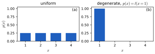
fig_2_1. Download: PDF · SVG2.2.2 Continuous random variables
pp. 36–38 For \(X\in\mathbb{R}\) one cannot list the values, so probabilities are attached to intervals. With \(A=(X\le a)\), \(B=(X\le b)\), \(C=(a<X\le b)\) and \(B=A\vee C\) exclusive, the sum rule gives \(\Pr(B)=\Pr(A)+\Pr(C)\) (2.9), so \(\Pr(C)=\Pr(B)-\Pr(A)\) (2.10). The cumulative distribution function (cdf) is
\[ P(x)\triangleq\Pr(X\le x),\qquad \Pr(a<X\le b)=P(b)-P(a), \tag{2.11, 2.12} \]non-decreasing, and the probability density function (pdf) is its derivative, \(p(x)\triangleq\frac{\d}{\d x}P(x)\) (2.13), so that
\[ \Pr(a<X\le b)=\int_a^bp(x)\,\d x,\qquad \Pr(x<X\le x+\d x)\approx p(x)\,\d x. \tag{2.14, 2.15} \]The quantile function (inverse cdf, ppf) is \(P^{-1}(q)\), the value \(x_q\) with \(\Pr(X\le x_q)=q\); \(P^{-1}(1/2)\) is the median and \(P^{-1}(1/4),P^{-1}(3/4)\) the quartiles. For the standard normal cdf \(\Phi\), the central interval \[ (\Phi^{-1}(\alpha/2),\Phi^{-1}(1-\alpha/2)) \] carries probability \(1-\alpha\), and for \(\alpha=0.05\)
\[ \big(\Phi^{-1}(0.025),\Phi^{-1}(0.975)\big)=(-1.96,\,1.96). \tag{2.16} \]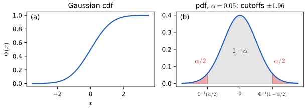
fig_2_2. Download: PDF · SVGFilling the gap 2.3: when the pdf exists, why it can exceed 1, and how the quantile function generates samples pp. 37–38, 58
The book notes "this derivative does not always exist" and that "the pdf at a point can be larger than 1" (for example \(\N(0\given0,0.1)=3.99\)), and defines the quantile function only for strictly increasing cdfs. Three precise statements.
Derivation
(a) Existence. A cdf is non-decreasing and right-continuous, hence differentiable almost everywhere, but it may have jumps (discrete part) or be continuous without a density (singular part, such as the Cantor function). A pdf exists exactly when \(P\) is absolutely continuous, i.e. \(P(x)=\int_{-\infty}^xp(t)\,\d t\) for some \(p\ge0\), which is the property used in (2.14).
(b) Values above 1. Only \(\int p=1\) is required, not \(p\le1\): \[ \Pr(x<X\le x+\d x)\approx p(x)\,\d x \] is a probability, \(p(x)\) a probability per unit length. The uniform density on \([0,\tfrac1{10}]\) equals 10 on its support. The Gaussian with standard deviation \(\sigma\) has peak \(1/(\sqrt{2\pi}\sigma)\), which is 3.99 for \(\sigma=0.1\) (and 1.26 for variance 0.1; see the note on notation).
(c) The generalised inverse. For any cdf define \(P^{-1}(q)=\inf\{x:P(x)\ge q\}\), \(0<q<1\); it coincides with the ordinary inverse when \(P\) is strictly increasing and continuous. Then \(P^{-1}(q)\le x\iff q\le P(x)\) (by right-continuity of \(P\)). Hence if \(U\sim\mathrm{Unif}(0,1)\),
\[ \Pr\big(P^{-1}(U)\le x\big)=\Pr\big(U\le P(x)\big)=P(x), \]so \(P^{-1}(U)\) has cdf \(P\): inverse-cdf sampling. Conversely, if \(X\) has a continuous cdf \(P\) then \(P(X)\sim\mathrm{Unif}(0,1)\) (the probability integral transform). ∎
2.2.3 Sets of related random variables
pp. 38–39 For two variables the joint distribution is \(p(x,y)=p(X=x,Y=y)\); for finite state spaces it is a table summing to one. Summing out gives the marginal (the sum rule, or rule of total probability), the conditional is a ratio, and rearranging gives the product rule:
\[ p(X=x)=\sum_yp(X=x,Y=y),\qquad p(y\given x)=\frac{p(x,y)}{p(x)},\qquad p(x,y)=p(x)p(y\given x). \tag{2.17, 2.18, 2.19} \]Iterating the product rule gives the chain rule:
\[ p(x_{1:D})=p(x_1)p(x_2\given x_1)p(x_3\given x_1,x_2)\cdots p(x_D\given x_{1:D-1}). \tag{2.20} \]Filling the gap 2.4: the chain rule by induction, and the parameter count of Figure 2.3 pp. 38–39
Derivation
Chain rule. For \(D=1\) it is trivial; for \(D=2\) it is (2.19). Assume it for \(D-1\) variables. Apply the product rule (2.19) with \(x=x_{1:D-1}\) and \(y=x_D\): \[ p(x_{1:D})=p(x_{1:D-1})\,p(x_D\given x_{1:D-1}), \] then expand the first factor by the induction hypothesis. The order of the variables is arbitrary, so any permutation gives another valid factorisation.
Counting parameters (Figure 2.3). A general joint pmf on a \(6\times5\) grid has 30 non-negative entries that sum to 1: \(30-1=29\) free numbers. If \(X\indep Y\), \(p(x,y)=p(x)p(y)\) needs the marginal of \(X\) (\(6-1=5\) free numbers) and of \(Y\) (\(5-1=4\)), so 9 in all. For \(D\) variables with \(K\) states, the full joint has \(K^D-1\) free numbers and a fully independent model only \(D(K-1)\): exponential versus linear, which is why conditional independence assumptions (Section 2.2.4, Chapter 4) are the basis of tractable models. ∎
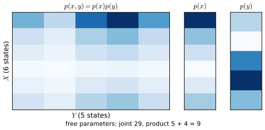
fig_2_3. Reproduces Murphy (2022), Figure 2.3 (with random marginals). Download: PDF · SVG2.2.4 Independence and conditional independence
pp. 39–40 \(X\) and \(Y\) are (marginally) independent, \(X\indep Y\), iff \(p(X,Y)=p(X)p(Y)\) (2.21); variables \(X_1,\dots,X_n\) are mutually independent if for every subset the joint is the product of the marginals (2.22); and \(X\indep Y\given Z\) iff \[ p(X,Y\given Z)=p(X\given Z)p(Y\given Z) \] (2.23).
Result 2.1 (mutual independence needs only the full product; pairwise is weaker; Exercise 2.2) p. 39, (2.22), (2.180)–(2.183)
(a) \(X_1,\dots,X_n\) are mutually independent iff \(p(x_1,\dots,x_n)=\prod_ip(x_i)\) for all values. (b) Pairwise independence does not imply mutual independence.
Proof
(a) "⇒" is the case of the full subset in (2.22). "⇐": summing the product over the variables outside a subset \(S\), \[ \sum_{x_j,\,j\notin S}\prod_ip(x_i)=\prod_{i\in S}p(x_i)\cdot\prod_{j\notin S}\sum_{x_j}p(x_j)=\prod_{i\in S}p(x_i), \] which is (2.22) for \(S\). In particular the book's four equations for \(X_1,X_2,X_3\) are not independent conditions: the three pairwise ones follow from the triple product.
(b) Let \(X_1,X_2\) be independent fair bits and \(X_3=X_1\oplus X_2\). Each pair is uniform on \(\{0,1\}^2\), hence independent, with marginals uniform. But \(p(1,1,1)=0\ne\tfrac18=p(1)p(1)p(1)\), because \(X_3\) is a function of the other two. ∎
See also (companion course): Section 1.5, independent events (pairwise versus mutual independence, with a demo).
2.2.5 Moments of a distribution
pp. 40–42 The mean (expected value) is \(\E[X]=\int x\,p(x)\,\d x\) (2.24), or \(\sum_xx\,p(x)\) (2.25), provided the integral converges absolutely (the Cauchy distribution of Section 2.7.2 has no mean). It is linear:
\[ \E[aX+b]=a\E[X]+b,\qquad \E\Big[\sum_{i=1}^nX_i\Big]=\sum_{i=1}^n\E[X_i],\qquad \E\Big[\prod_{i=1}^nX_i\Big]=\prod_{i=1}^n\E[X_i]\ \ (\text{independent}). \tag{2.26, 2.27, 2.28} \]The variance is \[ \var[X]=\E[(X-\mu)^2]=\E[X^2]-\mu^2 \] (2.29)–(2.30), so \(\E[X^2]=\sigma^2+\mu^2\) (2.31); the standard deviation \(\sqrt{\var[X]}=\sigma\) (2.32) has the units of \(X\). Then
\[ \var[aX+b]=a^2\var[X],\qquad \var\Big[\sum_{i=1}^nX_i\Big]=\sum_{i=1}^n\var[X_i]\ \ (\text{independent}), \tag{2.33, 2.34} \] \[ \var\Big[\prod_{i=1}^nX_i\Big]=\prod_i(\sigma_i^2+\mu_i^2)-\prod_i\mu_i^2\ \ (\text{independent}). \tag{2.35--2.39} \]The mode is \(x^*=\arg\max_xp(x)\) (2.40); it need not be unique (Figure 2.4) and may be a poor summary.
Filling the gap 2.5: proofs of (2.26)–(2.28), (2.30), (2.33)–(2.34) and (2.35)–(2.39) pp. 40–41
The book states (2.26)–(2.28) and (2.33)–(2.34) without proof and derives the product formula (2.35)–(2.39) using independence silently in step (2.37).
Derivation
Linearity (2.26), (2.27). For a joint density \(p(x_1,\dots,x_n)\) with marginals \(p_i\): \[ \E[\sum_iX_i]=\int\!\cdots\!\int\sum_ix_i\,p(x_{1:n})\,\d x_{1:n}=\sum_i\int x_ip_i(x_i)\,\d x_i, \] integrating the other variables out of each term (sum rule). No independence is used. \(\E[aX+b]=a\E[X]+b\) is the case \(n=1\) with the constant \(b\) integrating to \(b\) (all assuming the means exist).
Product (2.28). If the \(X_i\) are independent, \(p(x_{1:n})=\prod_ip_i(x_i)\), so the \(n\)-fold integral of \(\prod_ix_i\,p_i(x_i)\) is the product of the \(n\) one-dimensional integrals, \(\prod_i\E[X_i]\) (Fubini, using integrability of each factor). Independence is essential: \(\E[X\cdot X]=\E[X^2]\ne\E[X]^2\).
(2.30). Expanding the square, \[ \E[(X-\mu)^2]=\E[X^2]-2\mu\E[X]+\mu^2=\E[X^2]-\mu^2 \] (linearity and \(\E[X]=\mu\)).
(2.33), (2.34). \[ \var[aX+b]=\E[(aX+b-a\mu-b)^2]=a^2\E[(X-\mu)^2]. \] For the sum, let \(S=\sum_iX_i\); then \[ \var[S]=\E[(\sum_i(X_i-\mu_i))^2]=\sum_i\var[X_i]+\sum_{i\ne j}\cov[X_i,X_j], \] and \[ \cov[X_i,X_j]=\E[X_iX_j]-\mu_i\mu_j=0 \] for independent variables by (2.28). Without independence the covariances remain: \[ \var[X+Y]=\var[X]+\var[Y]+2\cov[X,Y] \] (2.187, Exercise 2.6).
(2.35)–(2.39). By (2.30) applied to \(\prod_iX_i\): \[ \var[\prod_iX_i]=\E[(\prod_iX_i)^2]-(\E[\prod_iX_i])^2. \] The variables \(X_i^2\) are independent (functions of independent variables), so (2.28) gives \[ \E[\prod_iX_i^2]=\prod_i\E[X_i^2]=\prod_i(\sigma_i^2+\mu_i^2), \] and again (2.28) gives \(\E[\prod_iX_i]=\prod_i\mu_i\). Check: for independent \(X_1\sim\N(1,4)\), \(X_2\sim\N(-1,1)\), \(X_3\sim\mathrm{Unif}(0,2)\) the formula gives \((4+1)(1+1)(\tfrac13+1)-1=12.33\), and a simulation of \(10^6\) products gives 12.3. ∎
2.2.5.4 Conditional moments
Result 2.2 (laws of total expectation and total variance) pp. 41–43, (2.41)–(2.50)
For random variables \(X\), \(Y\) with \(\E[X^2]<\infty\),
\[ \E[X]=\E_Y\big[\E[X\given Y]\big],\qquad \var[X]=\E_Y\big[\var[X\given Y]\big]+\var_Y\big[\E[X\given Y]\big]. \tag{2.41, 2.45} \]Proof (continuous or discrete, general)
Let \[ \mu(y)=\E[X\given Y=y]=\int x\,p(x\given y)\,\d x. \] Then \[ \E_Y[\mu(Y)]=\int\!\big(\int x\,p(x\given y)\,\d x\big)p(y)\,\d y=\iint x\,p(x,y)\,\d x\,\d y=\E[X], \] by the product rule (2.19) and the sum rule (2.17); the book's (2.42)–(2.43) is the discrete case. For the variance put \(s(y)=\E[X^2\given Y=y]\) and \[ \sigma^2(y)=\var[X\given Y=y]=s(y)-\mu(y)^2. \] Applying (2.41) to \(X^2\), \[ \E[X^2]=\E_Y[s(Y)]=\E_Y[\sigma^2(Y)]+\E_Y[\mu(Y)^2]. \] Then
\[ \var[X]=\E[X^2]-\E[X]^2=\E_Y[\sigma^2(Y)]+\big(\E_Y[\mu(Y)^2]-(\E_Y[\mu(Y)])^2\big)=\E_Y[\var[X\given Y]]+\var_Y[\mu(Y)], \]using \(\E[X]=\E_Y[\mu(Y)]\) once more: this is (2.46)–(2.48). ∎
Examples. (i) Lightbulbs: with \(\E[X\given Y=1]=5000\), \(\E[X\given Y=2]=4000\) and \(p(Y=1)=0.6\), \(\E[X]=5000(0.6)+4000(0.4)=4600\) (2.44). (ii) For a mixture \[ \sum_{y}\pi_y\N(x\given\mu_y,\sigma_y^2) \] the "within" term is \(\sum_y\pi_y\sigma_y^2\) and the "between" term is \(\sum_y\pi_y(\mu_y-\mu)^2\). For the mixture of Figure 2.4, with equal weights, means 0 and 2 and component standard deviations 0.5, they are \(0.25\) and \(1\) (2.49)–(2.50), so \(\var[X]=1.25\); a simulation of \(4\times10^5\) draws gives \(1.25\). The spread is dominated by which component generated the point, not by the spread within a component.
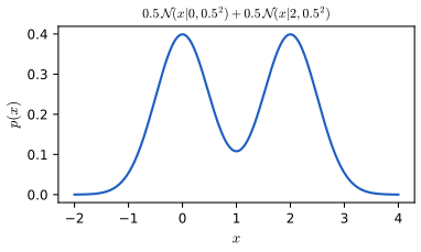
fig_2_4. Reproduces Murphy (2022), Figure 2.4. Download: PDF · SVGNote on notation in the book
The book defines \(\N(y\given\mu,\sigma^2)\) with the variance in the second slot (2.112), but then writes the mixture of Figure 2.4 as "\(0.5\N(x|0,0.5)+0.5\N(x|2,0.5)\)" and computes (2.49)–(2.50) with \(\sigma_1=\sigma_2=0.5\), i.e. with 0.5 as the standard deviation; likewise "\(\N(0|0,0.1)=3.99\)" (p. 58) is true for standard deviation 0.1 and false for variance 0.1, where the density at 0 is \(1/\sqrt{2\pi\cdot0.1}=1.26\). The numbers quoted are correct under the standard-deviation reading; only the notation is inconsistent. In these notes the second argument is always the variance, and the standard deviation is written out.
2.2.6 Limitations of summary statistics *
pp. 43–45 Means, variances and correlations discard most of a data set. Anscombe's quartet (1973) consists of four data sets of 10–11 points with identical low-order statistics but very different structure; the book then shows the Datasaurus Dozen, built by simulated annealing, and 1-d data sets with the same median and quartiles whose violin plots differ.
Filling the gap 2.6: why equal summary statistics mean equal regression lines, and how annealing manufactures the examples pp. 43–45
Derivation
The statistics determine the least-squares line. The line \(y=\hat\beta_0+\hat\beta_1x\) minimising \(\sum_n(y_n-\beta_0-\beta_1x_n)^2\) has slope \[ \hat\beta_1=\cov[x,y]/\var[x]=r\,s_y/s_x \] and intercept \[ \hat\beta_0=\bar y-\hat\beta_1\bar x, \] and its \(R^2=r^2\). So two data sets with the same \(\bar x,\bar y,s_x,s_y,r\) have the same line and the same \(R^2\) whatever their shape. For the four quartets: \(\bar x=9\), \(s_x^2=11\), \(\bar y=7.50\), \(s_y^2=4.12\), \(r=0.816\), fitted line \(y=3.00+0.500x\) (recomputed from the 44 published pairs). The book's footnote 4 notes that \(\var[x]=11\) is the unbiased estimate (divisor \(N-1\)); the maximum-likelihood divisor \(N\) gives 10.00 and 3.75.
Constructing look-alike data (Figure 2.6). Start from a data set and a target shape (a set of line segments). Repeat: pick a point, propose a small random move, accept it if the means, standard deviations and correlation are unchanged to the stated tolerance and if the point is closer to the shape (or, with a probability \(\exp(-\Delta/T)\) that falls as the temperature \(T\) is cooled, if it is not). The accepted moves move the cloud onto the shape while keeping the statistics frozen. The code updates the five sums \[ \sum x,\sum y,\sum x^2,\sum y^2,\sum xy \] in \(O(1)\) per move. ∎
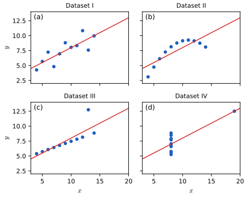
fig_2_5. Reproduces Murphy (2022), Figure 2.5. Download: PDF · SVG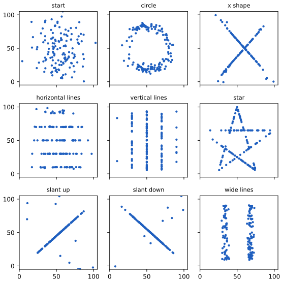
fig_2_6. Reproduces the idea of Murphy (2022), Figure 2.6. Download: PDF · SVG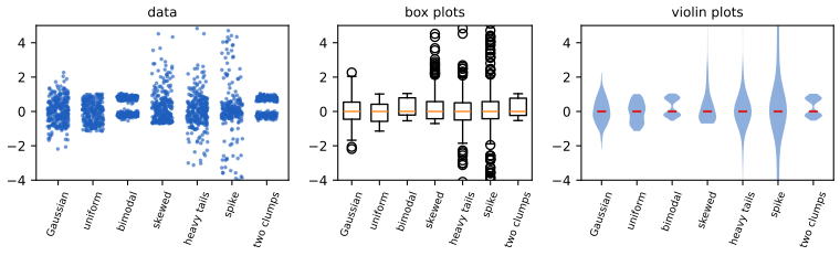
fig_2_7. Download: PDF · SVG2.3 Bayes' rule
pp. 44–45 Bayes' rule computes the distribution of an unknown \(H\) given observed data \(Y=y\):
\[ p(H=h\given Y=y)=\frac{p(H=h)\,p(Y=y\given H=h)}{p(Y=y)}, \tag{2.51} \]which follows from the two ways of factorising the joint, \[ p(h\given y)p(y)=p(h)p(y\given h)=p(h,y) \] (2.52). The terms are the prior \(p(H)\), the observation distribution \(p(Y\given H=h)\), which as a function of \(h\) at the observed \(y\) is the likelihood (not a distribution in \(h\)), the marginal likelihood \(p(Y=y)=\sum_{h'}p(h')p(y\given h')\) (2.53), and the posterior. In words, posterior \(\propto\) prior \(\times\) likelihood (2.54).
Result 2.3 (Bayes' rule in odds form, sequential updating, and the break-even prior) pp. 45–47, (2.51)–(2.60)
For a binary hypothesis \(H\in\{0,1\}\) and a binary test with true positive rate \(\mathrm{TPR}=p(Y=1\given H=1)\) and false positive rate \(\mathrm{FPR}=p(Y=1\given H=0)\):
\[ \underbrace{\frac{p(H=1\given Y=1)}{p(H=0\given Y=1)}}_{\text{posterior odds}}=\underbrace{\frac{p(H=1)}{p(H=0)}}_{\text{prior odds}}\times\underbrace{\frac{\mathrm{TPR}}{\mathrm{FPR}}}_{\text{likelihood ratio}} . \]If \(n\) tests are conditionally independent given \(H\) and all positive, the odds are multiplied by \((\mathrm{TPR}/\mathrm{FPR})^n\). The posterior after one positive test exceeds \(1/2\) iff the prior exceeds \[ \mathrm{FPR}/(\mathrm{TPR}+\mathrm{FPR}). \]
Proof
Dividing (2.51) for \(h=1\) by (2.51) for \(h=0\) cancels the common denominator \(p(Y=y)\): this is the odds form. Applying the rule twice, with the posterior after the first test as the prior of the second, and using \[ p(y_1,y_2\given h)=p(y_1\given h)p(y_2\given h), \] multiplies the odds by the likelihood ratio of each test; the result does not depend on the order, and equals the batch update with both observations at once. The odds exceed 1 iff \[ p(H=1)\,\mathrm{TPR}>p(H=0)\,\mathrm{FPR}, \] i.e. \[ \pi\,\mathrm{TPR}>(1-\pi)\mathrm{FPR}, \] i.e. \[ \pi>\mathrm{FPR}/(\mathrm{TPR}+\mathrm{FPR}). \] ∎
2.3.1 Example: Testing for COVID-19
pp. 46–47 A test has sensitivity (TPR) 0.875 and specificity (TNR) 0.975, so FNR \(=0.125\), FPR \(=0.025\) (Table 2.1), and the prior (prevalence) is \(p(H=1)=0.1\). A positive result gives
\[ p(H=1\given Y=1)=\frac{\mathrm{TPR}\times\text{prior}}{\mathrm{TPR}\times\text{prior}+\mathrm{FPR}\times(1-\text{prior})}=\frac{0.875\times0.1}{0.875\times0.1+0.025\times0.9}=0.795, \tag{2.55--2.57} \]and a negative result gives
\[ p(H=1\given Y=0)=\frac{0.125\times0.1}{0.125\times0.1+0.975\times0.9}=0.014 \tag{2.58--2.60} \]With prevalence 1% the two posteriors fall to 26% and 0.13%. The natural-frequency explanation: in 100,000 people, 1000 are infected and 875 of them test positive, while \(0.025\times99{,}000=2475\) healthy people also test positive, so \(875/(875+2475)=0.26\). By Result 2.3 a positive test is more likely to be a true than a false positive only above the break-even prevalence \(0.025/(0.875+0.025)=2.8\%\), and the likelihood ratio of a positive test is \(0.875/0.025=35\): two independent positives at 10% prior give odds \(\tfrac19\cdot35^2=136\), i.e. 99.3%.
See also (companion course): Section 1.7, Bayes' theorem and base rates and its demo.
2.3.2 Example: The Monty Hall problem
pp. 47–48 Three doors hide one prize. You pick door 1, the host opens a door that you did not pick and that hides no prize, and you may stay or switch. Let \(H_i\) be "the prize is behind door \(i\)", with \(P(H_i)=\tfrac13\) (2.61), and \(Y\) the door the host opens. If the prize is behind door 1 the host chooses between doors 2 and 3 at random; otherwise his choice is forced (2.62). After \(Y=3\), \[ P(Y=3)=\tfrac12\cdot\tfrac13+1\cdot\tfrac13+0=\tfrac12 \] and
\[ P(H_1\given Y=3)=\tfrac13,\qquad P(H_2\given Y=3)=\tfrac23,\qquad P(H_3\given Y=3)=0, \tag{2.63--2.65} \]so switching doubles the chance of winning (Table 2.2). The book's intuition is the million-door variant.
Result 2.4 (Monty Hall with \(n\) doors and two kinds of host) pp. 47–48, (2.61)–(2.65); Exercise 2.11
You pick door 1 among \(n\ge3\). (a) Informed host: he knows the prize, and opens \(n-2\) of the other doors, none hiding the prize, leaving one other door \(j\) closed. Then \(P(\text{prize at }1)=1/n\) and \(P(\text{prize at }j)=(n-1)/n\). (b) Random host: he opens one of the other \(n-1\) doors uniformly at random, and it happens to hide no prize. Then each of the \(n-1\) doors still closed, including yours, has probability \(1/(n-1)\); staying and switching win equally often.
Proof
(a) Let \(E\) be the observed event "the host opened exactly the doors other than 1 and \(j\)". If the prize is at 1, the host opens any \(n-2\) of the \(n-1\) other doors, each set equally likely: \(P(E\given H_1)=1/(n-1)\). If the prize is at \(j\), the set is forced: \(P(E\given H_j)=1\). If the prize is at an opened door, \(P(E\given H_i)=0\). With the uniform prior, Bayes' rule gives \[ P(H_1\given E)=\dfrac{1/(n-1)}{1/(n-1)+1}=\dfrac1n \] and \(P(H_j\given E)=\dfrac{n-1}{n}\). For \(n=3\) this is (2.65).
(b) Let \(E\) be "the host opened door \(o\) and it was empty". \(P(E\given H_i)=\tfrac1{n-1}\) for every \(i\ne o\) (he picks \(o\) among \(n-1\) doors, and the prize is elsewhere) and \(0\) for \(i=o\). The \(n-1\) surviving hypotheses have equal prior and equal likelihood, hence equal posterior \(1/(n-1)\). ∎
The observation "door 3 is empty" is the same in both worlds; what differs is the probability that the host would have shown an empty door, which is the likelihood. The posterior depends on the data-generating process, not only on the data: this is the point of Exercise 2.11. In (b) a fraction \(1/n\) of the games ends with the host exposing the prize and is discarded; a simulation of 60,000 games with \(n=3\) keeps about two thirds and gives stay \(=\) switch \(\approx0.50\); an informed host gives 0.33 and 0.67.
See also (companion course): the Monty Hall demo in All of Statistics.
2.3.3 Inverse problems *
p. 49 Probability theory predicts outcomes \(y\) from a state \(h\); an inverse problem infers \(h\) from \(y\) by inverting the forward map \(h\mapsto y\). Such problems are typically ill-posed in Hadamard's sense (no unique solution, or not stable): many 3-D shapes give the same 2-D image (Figure 2.8, a drawing that is not reproduced here), and many intended meanings give the same sentence. Bayes' rule resolves the ambiguity not by finding the one correct \(h\) but by returning the whole posterior \[ p(h\given y)\propto p(y\given h)p(h) \]: the forward model \(p(y\given h)\) says what each \(h\) predicts, and the prior \(p(h)\) down-weights implausible ones. The same idea underlies regularised regression (a Gaussian prior on the weights is the ridge penalty) and Bayesian deconvolution.
2.4 Bernoulli and binomial distributions
2.4.1 Definition
pp. 49–50 A coin lands heads (\(Y=1\)) with probability \(\theta\in[0,1]\): \(Y\sim\mathrm{Ber}(\theta)\) with
\[ \mathrm{Ber}(y\given\theta)=\begin{cases}1-\theta&y=0\\\theta&y=1\end{cases}=\theta^y(1-\theta)^{1-y}. \tag{2.66--2.68} \]The number of heads \(s=\sum_{n=1}^N\mathbb{I}(y_n=1)\) in \(N\) independent tosses is binomial,
\[ \mathrm{Bin}(s\given N,\theta)=\binom Ns\theta^s(1-\theta)^{N-s},\qquad\binom Nk=\frac{N!}{(N-k)!\,k!}. \tag{2.69, 2.70} \]Result 2.5 (the binomial pmf, its normalisation and moments) pp. 49–50, (2.69)–(2.70)
If \(Y_1,\dots,Y_N\) are iid \(\mathrm{Ber}(\theta)\), then \(S=\sum_nY_n\) has the pmf (2.69), \[ \sum_{s=0}^N\mathrm{Bin}(s\given N,\theta)=1, \] \(\E[S]=N\theta\), \(\var[S]=N\theta(1-\theta)\).
Proof
A particular sequence with \(s\) heads has probability \(\theta^s(1-\theta)^{N-s}\) by independence and (2.68); the number of sequences with exactly \(s\) heads is the number of ways of choosing which \(s\) of the \(N\) positions are heads, \(N!/(s!(N-s)!)\). Summing over \(s\) and using the binomial theorem, \[ \sum_s\binom Ns\theta^s(1-\theta)^{N-s}=(\theta+1-\theta)^N=1. \] For one toss \(\E[Y]=\theta\) and \(\E[Y^2]=\theta\) (since \(Y^2=Y\)), so \(\var[Y]=\theta-\theta^2\); then linearity (2.27) and (2.34) for independent summands give the mean and variance of \(S\). For \(N=1\), (2.69) is (2.68). ∎
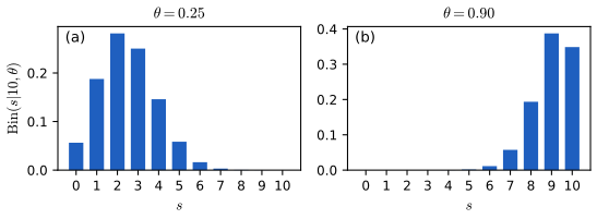
fig_2_9. Reproduces Murphy (2022), Figure 2.9. Download: PDF · SVG2.4.2 Sigmoid (logistic) function
pp. 50–52 To predict a binary \(y\) from inputs \(x\) one uses \[ p(y\given x,\theta)=\mathrm{Ber}(y\given f(x;\theta)) \] (2.71). To avoid constraining \(f\in[0,1]\), let \(f\) be unconstrained and pass it through the sigmoid (logistic function) \(\sigma(a)=1/(1+e^{-a})\) (2.72, 2.79), a smooth version of the Heaviside step \(\mathbb{I}(a>0)\) (2.80):
\[ p(y=1\given x,\theta)=\sigma(a)=\frac{e^a}{1+e^a},\quad p(y=0\given x,\theta)=\sigma(-a)=\frac1{1+e^a},\qquad a=f(x;\theta). \tag{2.78, 2.81, 2.82} \]The unconstrained \(a\) is the log-odds \(a=\log\frac p{1-p}\) (2.83), and \(\mathrm{logit}(p)=\sigma^{-1}(p)\) (2.85).
Result 2.6 (properties of the sigmoid, Table 2.3) p. 51, (2.72)–(2.77)
For all real \(x\) and \(p\in(0,1)\): (i) \[ \sigma(x)=\dfrac1{1+e^{-x}}=\dfrac{e^x}{1+e^x}; \] (ii) \(\sigma'(x)=\sigma(x)(1-\sigma(x))\); (iii) \(1-\sigma(x)=\sigma(-x)\); (iv) \[ \sigma^{-1}(p)=\log\frac p{1-p}=\mathrm{logit}(p); \] (v) \(\sigma_+(x)=\log(1+e^x)\) (softplus) has \(\sigma_+'(x)=\sigma(x)\); (vi) \(\log\sigma(x)=-\sigma_+(-x)\). The sigmoid maps \(\mathbb{R}\) onto the open interval \((0,1)\), strictly increasing.
Proof
(i) Multiply numerator and denominator by \(e^x\). (ii) \[ \sigma'=\dfrac{e^{-x}}{(1+e^{-x})^2}=\dfrac1{1+e^{-x}}\cdot\dfrac{e^{-x}}{1+e^{-x}}=\sigma(x)(1-\sigma(x)), \] since \(1-\sigma=e^{-x}/(1+e^{-x})\). (iii) \[ 1-\sigma(x)=\dfrac{e^{-x}}{1+e^{-x}}=\dfrac1{e^x+1}=\sigma(-x). \] (iv) If \(p=\sigma(a)\) then \(p/(1-p)=\sigma(a)/\sigma(-a)=e^a\), so \(a=\log\frac p{1-p}\). (v) \[ \frac{\d}{\d x}\log(1+e^x)=e^x/(1+e^x)=\sigma(x). \] (vi) \[ \log\sigma(x)=-\log(1+e^{-x})=-\sigma_+(-x). \] Since \(\sigma'>0\), \(\sigma\to0\) as \(x\to-\infty\) and \(\to1\) as \(x\to\infty\), the range is \((0,1)\); the book's "maps to \([0,1]\)" is true only up to the closure. The derivative (ii) is at most \(1/4\) (attained at 0), which is the source of vanishing gradients in deep networks. ∎
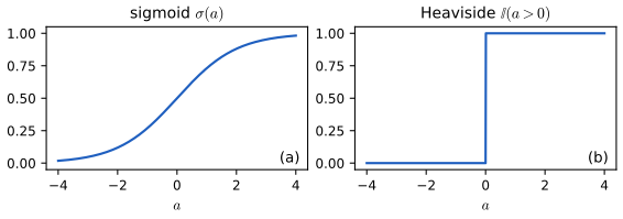
fig_2_10. Reproduces Murphy (2022), Figure 2.10. Download: PDF · SVG2.4.3 Binary logistic regression
pp. 52–53 With a linear predictor \[ f(x;\theta)=\mathbf{w}^\T\mathbf{x}+b, \]
\[ p(y=1\given\mathbf{x};\theta)=\sigma(\mathbf{w}^\T\mathbf{x}+b)=\frac1{1+e^{-(\mathbf{w}^\T\mathbf{x}+b)}} \tag{2.86, 2.87} \]is logistic regression. The decision boundary is \(\{x:\mathbf{w}^\T\mathbf{x}+b=0\}\), where \(p=\tfrac12\); the confidence grows with the distance from it. A linear regression of a 0/1 target would produce "probabilities" outside \([0,1]\), which is why the sigmoid is used.
Result 2.7 (the logistic-regression likelihood is concave; Newton's method) p. 53; Chapter 10
For data \((\mathbf{x}_n,y_n)\), \(y_n\in\{0,1\}\), let \[ p_n=\sigma(\mathbf{w}^\T\mathbf{x}_n+b) \] and \[ \tilde{\mathbf{x}}_n=(1,\mathbf{x}_n), \] \(\boldsymbol\theta=(b,\mathbf{w})\). The negative log-likelihood
\[ \mathrm{NLL}(\boldsymbol\theta)=-\sum_n\big[y_n\log p_n+(1-y_n)\log(1-p_n)\big]\quad\text{has} \] \[ \nabla\mathrm{NLL}=\sum_n(p_n-y_n)\tilde{\mathbf{x}}_n,\qquad \nabla^2\mathrm{NLL}=\sum_np_n(1-p_n)\tilde{\mathbf{x}}_n\tilde{\mathbf{x}}_n^\T\succeq0, \]so the NLL is convex, any stationary point is a global minimum, and Newton's method \[ \boldsymbol\theta\leftarrow\boldsymbol\theta-(\nabla^2\mathrm{NLL})^{-1}\nabla\mathrm{NLL} \] (iteratively reweighted least squares) finds it. If the classes are linearly separable the minimum is not attained (the weights diverge); a penalty \(\frac\lambda2\|\mathbf{w}\|^2\) restores a unique solution.
Proof
With \(a_n=\mathbf{w}^\T\mathbf{x}_n+b\), \[ -\log p(y_n\given a_n)=-y_na_n+\sigma_+(a_n) \] (from \(\log\sigma(a)=a-\sigma_+(a)\) and \(\log(1-\sigma(a))=-\sigma_+(a)\), Result 2.6). By Result 2.6(v) its derivative in \(a_n\) is \(p_n-y_n\), so by the chain rule \[ \nabla\mathrm{NLL}=\sum_n(p_n-y_n)\tilde{\mathbf{x}}_n. \] Differentiating again with Result 2.6(ii), \[ \partial p_n/\partial\boldsymbol\theta=p_n(1-p_n)\tilde{\mathbf{x}}_n, \] gives the Hessian. For any \(\mathbf{v}\), \[ \mathbf{v}^\T\nabla^2\mathrm{NLL}\,\mathbf{v}=\sum_np_n(1-p_n)(\mathbf{v}^\T\tilde{\mathbf{x}}_n)^2\ge0 \]: positive semi-definite, so NLL is convex. Separable data: if \(\mathbf{w}_0\) separates the classes, \[ \mathrm{NLL}(c\boldsymbol\theta_0)\to0 \] as \(c\to\infty\) without attaining it. ∎
Iris example (Figure 2.11). Using petal width as the feature and Virginica versus the rest as the label (150 flowers), Newton's method gives \(b=-21.13\), \(w=12.95\), so the maximum-likelihood decision boundary is \(x^*=-b/w=1.63\) cm; the gradient is zero to \(10^{-8}\) and the fit agrees with scikit-learn. The book reads off \(x^*\approx1.7\) from a fit with the library's default penalty, which shifts the boundary (we get 1.66 with penalty \(C=1\), 1.64 with \(C=10\) and 1.63 without a penalty).
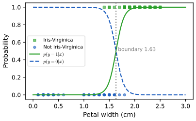
fig_2_11. Reproduces Murphy (2022), Figure 2.11. Download: PDF · SVGSee also (companion course): Bayesian and Probabilistic Machine Learning, Chapter 4 (logistic regression and its IRLS algorithm) and the logistic-regression demo.
2.5 Categorical and multinomial distributions
2.5.1 Definition
pp. 53–54 For a label \(y\in\{1,\dots,C\}\) the categorical distribution has one parameter per class,
\[ \mathrm{Cat}(y\given\boldsymbol\theta)=\prod_{c=1}^C\theta_c^{\mathbb{I}(y=c)}=\prod_c\theta_c^{y_c},\qquad\theta_c\ge0,\ \sum_c\theta_c=1 \tag{2.88, 2.89} \](the second form with the one-hot encoding \(y_c\)). The counts \(\mathbf{y}=(N_1,\dots,N_C)\) of \(N\) iid categorical trials are multinomial:
\[ \mathcal{M}(\mathbf{y}\given N,\boldsymbol\theta)=\binom N{N_1\ \cdots\ N_C}\prod_c\theta_c^{N_c},\qquad \binom N{N_1\cdots N_C}=\frac{N!}{N_1!N_2!\cdots N_C!}. \tag{2.90, 2.91} \]The multinomial coefficient counts the ways to divide \(N\) positions into groups of sizes \(N_1,\dots,N_C\) (choose \(N_1\) positions, then \(N_2\) of the remaining \(N-N_1\), and so on: \[ \binom N{N_1}\binom{N-N_1}{N_2}\cdots=N!/\prod N_c! \]). By the multinomial theorem \[ \sum_{\mathbf{N}}\mathcal{M}=(\sum_c\theta_c)^N=1, \] and \(\E[N_c]=N\theta_c\), \(\var[N_c]=N\theta_c(1-\theta_c)\) because \(N_c\sim\mathrm{Bin}(N,\theta_c)\). For \(N=1\) the multinomial is the categorical.
2.5.2 Softmax function
pp. 54–55 A conditional categorical model is \[ p(y\given\mathbf{x},\theta)=\mathrm{Cat}(y\given f(\mathbf{x};\theta)) \] (2.92), equivalently \(\mathcal{M}(y\given1,f)\) (2.93). To let \(f\) be unconstrained, pass the logits \(\mathbf{a}=f(\mathbf{x};\theta)\) through the softmax (multinomial logit):
\[ \mathrm{softmax}(\mathbf{a})_c=\frac{e^{a_c}}{\sum_{c'=1}^Ce^{a_{c'}}}. \tag{2.94} \]Result 2.8 (softmax: invariance, temperature limit, binary case, Jacobian, and the log-sum-exp trick) pp. 54–56, (2.94)–(2.105)
Let \[ \mathrm{lse}(\mathbf{a})=\log\sum_ce^{a_c}. \] (i) \[ \mathrm{softmax}(\mathbf{a})_c=\exp(a_c-\mathrm{lse}(\mathbf{a}))\in(0,1), \] the entries sum to 1, and \[ \mathrm{softmax}(\mathbf{a}+k\mathbf{1})=\mathrm{softmax}(\mathbf{a}) \] for any constant \(k\). (ii) If \(a_{c^*}\) is the unique maximum, \[ \mathrm{softmax}(\mathbf{a}/T)\to\mathbf{e}_{c^*} \] as \(T\to0^+\) (2.95), and \(\to\frac1C\mathbf{1}\) as \(T\to\infty\). (iii) For \(C=2\), \[ \mathrm{softmax}(\mathbf{a})_0=\sigma(a_0-a_1) \] (2.98). (iv) \[ \nabla\mathrm{lse}(\mathbf{a})=\mathrm{softmax}(\mathbf{a}) \] and the Jacobian of softmax is \[ \mathrm{diag}(\mathbf{p})-\mathbf{p}\mathbf{p}^\T \] with \[ \mathbf{p}=\mathrm{softmax}(\mathbf{a}). \] (v) For every \(m\), \[ \mathrm{lse}(\mathbf{a})=m+\log\sum_ce^{a_c-m} \] (2.100), and with \(m=\max_ca_c\), \[ \max_ca_c\le\mathrm{lse}(\mathbf{a})\le\max_ca_c+\log C. \] (vi) The cross-entropy of a label \(y\) under the softmax is \[ -\log p_y=\mathrm{lse}(\mathbf{a})-a_y. \]
Proof
(i) \[ e^{a_c}/\sum e^{a_{c'}}=\exp(a_c-\log\sum e^{a_{c'}}); \] the normalisation is built in; multiplying every \(e^{a_c}\) by \(e^k\) cancels. (ii) Write \[ \mathrm{softmax}(\mathbf{a}/T)_c=1/\sum_{c'}e^{(a_{c'}-a_c)/T}. \] For \(c=c^*\) every exponent \((a_{c'}-a_{c^*})/T\le0\), and \(\to-\infty\) for \(c'\ne c^*\), so the sum tends to 1. For \(c\ne c^*\) the term \(c'=c^*\) has exponent \((a_{c^*}-a_c)/T\to+\infty\), so the entry tends to 0. As \(T\to\infty\) all exponents tend to 0 and each entry to \(1/C\). (iii) \[ \dfrac{e^{a_0}}{e^{a_0}+e^{a_1}}=\dfrac1{1+e^{a_1-a_0}}=\sigma(a_0-a_1). \] The two-class model needs one weight vector \(\mathbf{w}_0-\mathbf{w}_1\); the \(C\)-class model is over-parametrised by the shift in (i), which does not change the predictions. (iv) \[ \partial\,\mathrm{lse}/\partial a_c=e^{a_c}/\sum e^{a_{c'}}=p_c. \] Then \[ \partial p_c/\partial a_d=p_c(\delta_{cd}-p_d). \] (v) \[ m+\log\sum e^{a_c-m}=m+\log(e^{-m}\sum e^{a_c})=\log\sum e^{a_c}. \] With \(m=\max a\) the sum \(\sum e^{a_c-m}\) lies in \([1,C]\): it contains the term \(e^0=1\) and no term exceeds 1, which gives the bounds, and no overflow can occur; terms that underflow are negligible next to the 1. (vi) \[ -\log p_y=-(a_y-\mathrm{lse}(\mathbf{a})). \] In the binary case, \(\log p_1=-\mathrm{lse}([0,-a])\) and \(\log p_0=-\mathrm{lse}([0,a])\) (2.104)–(2.105), by (iii). ∎
For \(\mathbf{a}=(3,0,1)\) the softmax is \((0.844,0.042,0.114)\) at \(T=1\), \((0.629,0.140,0.231)\) at \(T=2\), and \(\approx(0.34,0.33,0.33)\) at \(T=100\) (Figure 2.12).
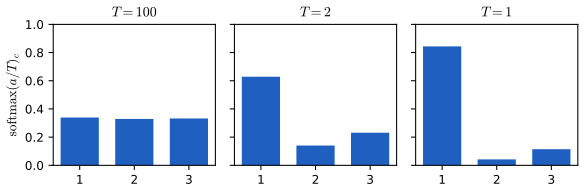
fig_2_12. Reproduces Murphy (2022), Figure 2.12. Download: PDF · SVG2.5.3 Multiclass logistic regression
pp. 55–56 With a linear predictor \[ \mathbf{a}=\mathbf{W}\mathbf{x}+\mathbf{b} \] (\(\mathbf{W}\) is \(C\times D\)),
\[ p(y\given\mathbf{x};\theta)=\mathrm{Cat}(y\given\mathrm{softmax}(\mathbf{W}\mathbf{x}+\mathbf{b})),\qquad p(y=c\given\mathbf{x};\theta)=\frac{e^{a_c}}{\sum_{c'}e^{a_{c'}}}. \tag{2.96, 2.97} \]Filling the gap 2.7: the multiclass NLL, its gradient, and linear decision boundaries pp. 55–56
The book fits this model to iris with two features and shows linear boundaries but does not derive the objective.
Derivation
With one-hot labels \(y_{nc}\) the NLL is \[ \sum_n\big[\mathrm{lse}(\mathbf{a}_n)-\sum_cy_{nc}a_{nc}\big] \] (Result 2.8(vi)), where \[ \mathbf{a}_n=\mathbf{W}\mathbf{x}_n+\mathbf{b}. \] By Result 2.8(iv) the gradient with respect to the logits is \(\mathbf{p}_n-\mathbf{y}_n\), so \[ \nabla_{\mathbf{W}}=\sum_n(\mathbf{p}_n-\mathbf{y}_n)\mathbf{x}_n^\T \] and \[ \nabla_{\mathbf{b}}=\sum_n(\mathbf{p}_n-\mathbf{y}_n). \] The function \(\mathrm{lse}\) is convex (its Hessian \[ \mathrm{diag}(\mathbf{p})-\mathbf{p}\mathbf{p}^\T \] is positive semi-definite: \[ \mathbf{v}^\T(\cdot)\mathbf{v}=\sum_cp_cv_c^2-(\sum_cp_cv_c)^2\ge0 \] by Jensen), and the logits are linear in the parameters, so the NLL is convex. The classes \(c\) and \(c'\) have equal probability where \(a_c=a_{c'}\), i.e. \[ (\mathbf{w}_c-\mathbf{w}_{c'})^\T\mathbf{x}+(b_c-b_{c'})=0 \]: a hyperplane, so every boundary between two classes is linear. Adding \(\frac\lambda2\|\mathbf{W}\|^2\) makes the minimiser unique (it removes the shift invariance and the separable-data divergence). Our fit with \(\lambda=0.1\) on petal length and width (150 flowers, L-BFGS with the exact gradient) classifies 96% of the flowers correctly and agrees with scikit-learn's \(C=10\) fit to \(10^{-4}\) in the predicted probabilities. ∎
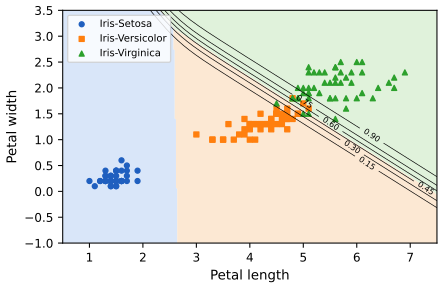
fig_2_13. Reproduces Murphy (2022), Figure 2.13. Download: PDF · SVG2.5.4 Log-sum-exp trick
pp. 56–57 Computing \(p_c=e^{a_c}/Z(\mathbf{a})\) naively fails for large \(|a_c|\): for \(\mathbf{a}=(1000,1001,1000)\) the sum overflows (\(e^{1000}=\infty\) in double precision) and for \(\mathbf{a}=(-1000,-999,-1000)\) it underflows to \(Z=0\). Result 2.8(v) fixes this: compute \(\mathrm{lse}(\mathbf{a})\) with \(m=\max_ca_c\) (2.100)–(2.101) and then \[ p_c=\exp(a_c-\mathrm{lse}(\mathbf{a})) \] (2.102). For \(\mathbf{a}=(0,1,0)\), \(Z=4.71\), and the stable and naive values agree. For the loss, one never forms \(p_c\): by Result 2.8(vi) the cross-entropy is \(\mathrm{lse}(\mathbf{a})-a_y\), and for the binary case \[ L=-[\mathbb{I}(y=0)\log p_0+\mathbb{I}(y=1)\log p_1] \] (2.103) is computed from \(\log p_1=-\mathrm{lse}([0,-a])\) and \(\log p_0=-\mathrm{lse}([0,a])\) (2.104)–(2.105), i.e. from the softplus, which is numerically stable.
2.6 Univariate Gaussian (normal) distribution
2.6.1 Cumulative distribution function
p. 57 The cdf of a real random variable is \(P(y)=\Pr(Y\le y)\) (2.106), and \(\Pr(a<Y\le b)=P(b)-P(a)\) (2.107); for the Gaussian,
\[ \Phi(y;\mu,\sigma^2)\triangleq\int_{-\infty}^y\N(z\given\mu,\sigma^2)\,\d z=\tfrac12\Big[1+\mathrm{erf}\Big(\frac{y-\mu}{\sigma\sqrt2}\Big)\Big],\qquad\mathrm{erf}(u)=\frac2{\sqrt\pi}\int_0^ue^{-t^2}\,\d t. \tag{2.108, 2.109} \]\(\mu\) is the mean (and mode), \(\sigma^2\) the variance, \(\lambda=1/\sigma^2\) the precision; \(\mu=0,\sigma=1\) is the standard normal with density \(\phi\) and cdf \(\Phi\). The quantile function \(\Phi^{-1}\) is the probit function; the central 95% interval is \(\pm1.96\) (2.110), often rounded to \(\mu\pm2\sigma\).
2.6.2 Probability density function
\[ \N(y\given\mu,\sigma^2)\triangleq\frac1{\sqrt{2\pi\sigma^2}}\exp\Big(-\frac1{2\sigma^2}(y-\mu)^2\Big)=\phi(y;\mu,\sigma^2). \tag{2.111, 2.112} \]Result 2.9 (the Gaussian density: normalisation, mean, variance, cdf; Exercise 2.12) pp. 57–58, (2.108)–(2.119), (2.191)–(2.193)
(i) \[ \int_{-\infty}^\infty e^{-x^2/(2\sigma^2)}\d x=\sqrt{2\pi\sigma^2}, \] so \(\N(y\given\mu,\sigma^2)\) integrates to 1. (ii) \(\E[Y]=\mu\), \(\var[Y]=\sigma^2\), \(\E[Y^2]=\sigma^2+\mu^2\) (2.118). (iii) \[ \Phi(y;\mu,\sigma^2)=\frac12[1+\mathrm{erf}((y-\mu)/(\sigma\sqrt2))]. \] (iv) The peak density is \(1/\sqrt{2\pi\sigma^2}\), which exceeds 1 when \(\sigma<1/\sqrt{2\pi}=0.399\).
Proof
(i) Let \[ Z=\int_{-\infty}^\infty e^{-x^2/2\sigma^2}\d x. \] Then \[ Z^2=\iint e^{-(x^2+y^2)/2\sigma^2}\d x\,\d y. \] Change to polar coordinates \(x=r\cos\theta\), \(y=r\sin\theta\), for which \(\d x\,\d y=r\,\d r\,\d\theta\) (Section 2.8.3) and \(x^2+y^2=r^2\):
\[ Z^2=\int_0^{2\pi}\d\theta\int_0^\infty re^{-r^2/2\sigma^2}\d r=2\pi\Big[-\sigma^2e^{-r^2/2\sigma^2}\Big]_0^\infty=2\pi\sigma^2, \]using \[ \frac{\d}{\d r}(-\sigma^2e^{-r^2/2\sigma^2})=re^{-r^2/2\sigma^2} \] (the book's hint with \(u=e^{-r^2/2\sigma^2}\)). Since the integrand is positive, \(Z=\sqrt{2\pi\sigma^2}\); (2.191)–(2.193) is this computation. The interchange of the order of integration is justified by Tonelli's theorem (non-negative integrand).
(ii) The integrand of \[ \E[Y-\mu]=\int(y-\mu)\N(y\given\mu,\sigma^2)\d y \] is odd about \(\mu\) and absolutely integrable, so the integral is 0. For the variance, with \(u=(y-\mu)/\sigma\), \[ \var[Y]=\sigma^2\int u^2\phi(u)\,\d u \] and integration by parts with \(u\phi(u)=-\phi'(u)\) gives \[ \int u^2\phi(u)\,\d u=[-u\phi(u)]_{-\infty}^\infty+\int\phi(u)\,\d u=0+1, \] so \(\var[Y]=\sigma^2\); then (2.118) is (2.31).
(iii) With \(u=(z-\mu)/(\sigma\sqrt2)\), \[ \Phi=\frac1{\sqrt\pi}\int_{-\infty}^{(y-\mu)/(\sigma\sqrt2)}e^{-u^2}\d u=\frac1{\sqrt\pi}\big[\int_{-\infty}^0+\int_0^{(y-\mu)/(\sigma\sqrt2)}\big], \] the first piece is \(\frac12\) by symmetry and (i), the second is \(\frac12\mathrm{erf}(\cdot)\). (iv) is the value at \(y=\mu\). ∎
As the interval shrinks, \[ \Pr(y\le Y\le y+\d y)\approx p(y)\,\d y \] (2.113)–(2.114); the density at a point can exceed 1 (Filling the gap 2.3), e.g. \(\N(0\given0,\sigma=0.1)=3.99\).
2.6.3 Regression
pp. 59 Letting the parameters of a Gaussian depend on an input gives a conditional density model
\[ p(y\given x;\theta)=\N\big(y\given f_\mu(x;\theta),f_\sigma(x;\theta)^2\big). \tag{2.120} \]With a fixed variance and a linear mean this is (homoskedastic) linear regression, \[ p(y\given\mathbf{x};\theta)=\N(y\given\mathbf{w}^\T\mathbf{x}+b,\sigma^2) \] (2.121). If the noise level also depends on the input, the model is heteroskedastic:
\[ p(y\given\mathbf{x};\theta)=\N\big(y\given\mathbf{w}_\mu^\T\mathbf{x}+b,\ \sigma_+(\mathbf{w}_\sigma^\T\mathbf{x})^2\big),\qquad\sigma_+(a)=\log(1+e^a), \tag{2.122, 2.123} \]where the softplus (Result 2.6) keeps the standard deviation positive. (The book's (2.122) writes \[ \sigma_+(\mathbf{w}_\sigma^\T\mathbf{x}) \] in the variance slot; the intended and the plotted quantity is the standard deviation, again the notation point of the note above.)
Result 2.10 (maximum likelihood for Gaussian regression) p. 59, (2.120)–(2.123)
(a) For (2.121) the maximum-likelihood \((\mathbf{w},b)\) minimise \[ \sum_n(y_n-\mathbf{w}^\T\mathbf{x}_n-b)^2 \] (least squares), for every value of \(\sigma^2\), and \[ \hat\sigma^2=\frac1N\sum_n(y_n-\hat{\mathbf{w}}^\T\mathbf{x}_n-\hat b)^2. \] (b) For (2.122) with \[ s_n=\sigma_+(\mathbf{w}_\sigma^\T\mathbf{x}_n) \] and residuals \[ r_n=y_n-\mathbf{w}_\mu^\T\mathbf{x}_n-b, \]
\[ \mathrm{NLL}=\sum_n\Big[\log s_n+\tfrac12\log2\pi+\frac{r_n^2}{2s_n^2}\Big],\qquad \frac{\partial\mathrm{NLL}}{\partial\mathbf{w}_\mu}=-\sum_n\frac{r_n}{s_n^2}\mathbf{x}_n,\quad \frac{\partial\mathrm{NLL}}{\partial\mathbf{w}_\sigma}=\sum_n\Big(\frac1{s_n}-\frac{r_n^2}{s_n^3}\Big)\sigma(\mathbf{w}_\sigma^\T\mathbf{x}_n)\,\mathbf{x}_n. \]The mean part is weighted least squares with weights \(1/s_n^2\): noisy points count less. The NLL is not jointly convex in \((\mathbf{w}_\mu,\mathbf{w}_\sigma)\), but for fixed \(\mathbf{w}_\sigma\) it is convex in \(\mathbf{w}_\mu\).
Proof
(a) \[ -\log\N(y_n\given m_n,\sigma^2)=\frac12\log2\pi\sigma^2+(y_n-m_n)^2/2\sigma^2 \]: for each fixed \(\sigma^2\) the NLL is an increasing affine function of the sum of squares, so the minimiser in \((\mathbf{w},b)\) does not depend on \(\sigma^2\). Substituting it and setting \[ \partial/\partial\sigma^2\big[\frac N2\log\sigma^2+\mathrm{SS}/(2\sigma^2)\big]=0 \] gives \(\hat\sigma^2=\mathrm{SS}/N\) (the maximum-likelihood, divisor-\(N\) estimate, biased downwards by \((N-D-1)/N\) for \(D\) inputs). (b) The NLL expression is the sum of the log of (2.120). Differentiating, \[ \partial(r_n^2/2s_n^2)/\partial\mathbf{w}_\mu=-r_n\mathbf{x}_n/s_n^2; \] and \[ \partial s_n/\partial\mathbf{w}_\sigma=\sigma(\mathbf{w}_\sigma^\T\mathbf{x}_n)\mathbf{x}_n \] (Result 2.6(v)) with \[ \partial(\log s_n+r_n^2/2s_n^2)/\partial s_n=1/s_n-r_n^2/s_n^3. \] ∎
Figure 2.14. We simulated 120 points with mean \(4+0.25x\) and a standard deviation growing with \(x\) (the book's data come from a TensorFlow Probability example and are not available). The constant-\(\sigma\) fit has NLL 219.6; the heteroskedastic fit has NLL 179.1 and its \(\pm2\sigma(x)\) band fans out with the data. The band plotted is the 95% predictive interval \[ [\mu(x)-2\sigma(x),\mu(x)+2\sigma(x)] \] for a new observation; the uncertainty in the noise-free line \(f_\mu(x;\theta)\) is smaller and comes from the uncertainty in the parameters (Section 11.7).
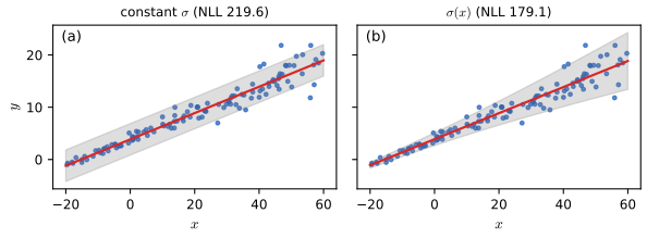
fig_2_14. Reproduces Murphy (2022), Figure 2.14. Download: PDF · SVG2.6.4 Why is the Gaussian distribution so widely used?
p. 60 Four reasons: it has two interpretable parameters (mean, variance); the central limit theorem (Section 2.8.6) makes it a good model of sums of many small effects such as noise; it has maximum entropy among distributions with given mean and variance; and it has convenient mathematics. The book defers the entropy statement to Section 3.4.4; here is the proof.
Result 2.11 (the Gaussian has maximum entropy for given mean and variance) p. 60; Section 3.4.4
Among all densities \(q\) on \(\mathbb{R}\) with mean \(\mu\) and variance \(\sigma^2\), the differential entropy \(h(q)=-\int q\log q\) is largest for \(q=\N(\mu,\sigma^2)\), with value \(\tfrac12\log(2\pi e\sigma^2)\).
Proof
Let \(g=\N(\mu,\sigma^2)\). Its log density is \[ \log g(x)=-\tfrac12\log(2\pi\sigma^2)-(x-\mu)^2/2\sigma^2. \] For any \(q\) with the stated mean and variance, \[ \int q\log g=-\tfrac12\log(2\pi\sigma^2)-\tfrac12=-\tfrac12\log(2\pi e\sigma^2), \] the same value as for \(q=g\). Then \(\KL(q\|g)=\int q\log(q/g)\ge0\) (Gibbs' inequality, Chapter 6) gives \(-h(q)-\int q\log g\ge0\), i.e. \[ h(q)\le-\int q\log g=\tfrac12\log(2\pi e\sigma^2)=h(g), \] with equality iff \(q=g\) almost everywhere. ∎
Historical note (Jaynes): the density was found by de Moivre before Laplace, and popularised by Gauss; the name "normal" is said to come from the normal equations of least squares.
2.6.5 Dirac delta function as a limiting case
p. 60 As \(\sigma\to0\), \[ \N(y\given\mu,\sigma^2)\to\delta(y-\mu) \] (2.124), the Dirac delta that is \(+\infty\) at 0, 0 elsewhere (2.125), with unit integral (2.126), and \(\delta_y(x)=\delta(x-y)\) (2.127)–(2.128). It is not a function but a distribution, defined by what it does under an integral: the sifting property \(\int f(y)\delta(x-y)\,\d y=f(x)\) (2.129).
Filling the gap 2.8: the delta function as a limit, and the sifting property p. 60
The book defines \(\delta\) by "\(\infty\) at 0 with unit integral", which no ordinary function satisfies (a function that is 0 almost everywhere integrates to 0). The right statement is a limit of integrals.
Derivation
Let \(f\) be bounded and continuous at \(x\), and \[ \phi_\sigma(y)=\N(y\given x,\sigma^2). \] Then \[ \big|\int f(y)\phi_\sigma(y)\,\d y-f(x)\big|=\big|\int(f(y)-f(x))\phi_\sigma(y)\,\d y\big| \] because \(\int\phi_\sigma=1\). Given \(\varepsilon>0\) choose \(\eta\) with \(|f(y)-f(x)|<\varepsilon\) for \(|y-x|<\eta\). The part of the integral over \(|y-x|<\eta\) is at most \(\varepsilon\); the part over \(|y-x|\ge\eta\) is at most \[ 2\sup|f|\cdot\Pr(|Y-x|\ge\eta)\le2\sup|f|\,\sigma^2/\eta^2\to0 \] (Chebyshev). Hence \(\int f\phi_\sigma\to f(x)\): the Gaussians converge to \(\delta(\cdot-x)\) in the sense of (2.129), and equally the variables converge in distribution to the constant \(x\). The same holds for any density rescaled as \(\sigma^{-1}\psi((y-x)/\sigma)\). The empirical distribution of Section 2.7.6 is a sum of such spikes. ∎
2.6.6 Truncated Gaussian distribution
p. 61 Restricting the Gaussian to an interval \((a,b)\) and renormalising gives
\[ \N(x\given\mu,\sigma^2,a,b)=\frac{\sigma^{-1}\phi\big(\frac{x-\mu}\sigma\big)}{\Phi\big(\frac{b-\mu}\sigma\big)-\Phi\big(\frac{a-\mu}\sigma\big)}\,\mathbb{I}(a<x<b). \]With \(a=0\) the support is the positive reals. The normalising constant is the probability the untruncated variable falls in \((a,b)\) (Section 2.2.2). The mean is \[ \mu+\sigma\dfrac{\phi(\alpha)-\phi(\beta)}{\Phi(\beta)-\Phi(\alpha)} \] with \(\alpha=\frac{a-\mu}\sigma\), \(\beta=\frac{b-\mu}\sigma\): \[ \int_\alpha^\beta u\phi(u)\,\d u=\phi(\alpha)-\phi(\beta) \] because \(u\phi(u)=-\phi'(u)\), and \(x=\mu+\sigma u\). It lies strictly between \(a\) and \(b\), and moves towards the interior relative to \(\mu\) when \(\mu\) is near an endpoint.
See also (companion course): Bayesian and Probabilistic Machine Learning, Section 2.3 (the Gaussian in full) and All of Statistics, Section 2.4.
2.7 Some other common univariate distributions *
2.7.1 Student t distribution
pp. 61–62 The Gaussian is sensitive to outliers; a robust alternative is the Student t distribution with location \(\mu\), scale \(\sigma>0\) (not the standard deviation) and degrees of freedom \(\nu>0\):
\[ \mathcal{T}(y\given\mu,\sigma^2,\nu)\propto\Big[1+\frac1\nu\Big(\frac{y-\mu}\sigma\Big)^2\Big]^{-\frac{\nu+1}2},\qquad \text{mean}=\text{mode}=\mu,\quad\var=\frac{\nu\sigma^2}{\nu-2}. \tag{2.130, 2.131} \]The mean exists for \(\nu>1\), the variance for \(\nu>2\). The density decays polynomially, not exponentially, so it has heavy tails.
Result 2.12 (Student as an infinite Gaussian mixture; moments; EM) pp. 61–62, (2.130)–(2.131)
Let \[ \lambda\sim\mathrm{Ga}(\nu/2,\nu/2) \] (shape, rate) and \[ y\given\lambda\sim\N(\mu,\sigma^2/\lambda). \] Then \(y\sim\mathcal{T}(\mu,\sigma^2,\nu)\), with normalising constant
\[ \mathcal{T}(y\given\mu,\sigma^2,\nu)=\frac{\Gamma(\frac{\nu+1}2)}{\Gamma(\frac\nu2)\sqrt{\nu\pi}\,\sigma}\Big[1+\frac1\nu\Big(\frac{y-\mu}\sigma\Big)^2\Big]^{-\frac{\nu+1}2}. \]The \(k\)-th absolute moment exists iff \(k<\nu\); the mean is \(\mu\) for \(\nu>1\), and \(\var[y]=\sigma^2\nu/(\nu-2)\) for \(\nu>2\). As \(\nu\to\infty\), \(\mathcal{T}\to\N(\mu,\sigma^2)\). For observations \(y_1,\dots,y_N\) and fixed \(\nu\), maximum likelihood for \((\mu,\sigma^2)\) is found by EM: with \(z_n=(y_n-\mu)/\sigma\), the E step sets \(w_n=\dfrac{\nu+1}{\nu+z_n^2}\) and the M step \(\mu=\sum_nw_ny_n/\sum_nw_n\), \[ \sigma^2=\frac1N\sum_nw_n(y_n-\mu)^2. \]
Proof
Marginal. \[ p(y)=\int_0^\infty\N(y\given\mu,\sigma^2/\lambda)\,\mathrm{Ga}(\lambda\given\tfrac\nu2,\tfrac\nu2)\,\d\lambda=\int_0^\infty\sqrt{\frac\lambda{2\pi\sigma^2}}e^{-\lambda z^2/2}\frac{(\nu/2)^{\nu/2}}{\Gamma(\nu/2)}\lambda^{\nu/2-1}e^{-\nu\lambda/2}\,\d\lambda \] with \(z=(y-\mu)/\sigma\). The \(\lambda\)-dependence is \[ \lambda^{(\nu+1)/2-1}e^{-\lambda(\nu+z^2)/2}, \] a gamma kernel with shape \((\nu+1)/2\) and rate \((\nu+z^2)/2\), whose integral is \[ \Gamma(\frac{\nu+1}2)\big(\frac{\nu+z^2}2\big)^{-(\nu+1)/2}. \] Collecting constants, \[ p(y)=\dfrac{(\nu/2)^{\nu/2}\Gamma(\frac{\nu+1}2)}{\sqrt{2\pi}\sigma\Gamma(\frac\nu2)}\Big(\dfrac{\nu+z^2}2\Big)^{-\frac{\nu+1}2}=\dfrac{\Gamma(\frac{\nu+1}2)}{\Gamma(\frac\nu2)\sqrt{\nu\pi}\sigma}\Big(1+\dfrac{z^2}\nu\Big)^{-\frac{\nu+1}2}, \] the stated density (so (2.130) is proportional with that constant).
Moments. By Result 2.2, \(\E[y]=\E[\mu]=\mu\) (when it exists) and \[ \var[y]=\E[\sigma^2/\lambda]+\var[\mu]=\sigma^2\E[1/\lambda]; \] for \(\lambda\sim\mathrm{Ga}(a,b)\), \(\E[1/\lambda]=b/(a-1)\) (Result 2.15, finite iff \(a>1\)), here \((\nu/2)/(\nu/2-1)=\nu/(\nu-2)\). Since the density behaves like \(|y|^{-(\nu+1)}\) in the tails, \(\int|y|^k|y|^{-(\nu+1)}\d y\) converges iff \(k<\nu\). As \(\nu\to\infty\), \(\lambda\) concentrates at its mean 1 (variance \(2/\nu\)), so \(y\to\N(\mu,\sigma^2)\).
EM. With \(\lambda_n\) as latent variables, the complete-data log-likelihood is \[ \sum_n[\tfrac12\log\lambda_n-\tfrac12\log\sigma^2-\lambda_nz_n^2/2]+\mathrm{const}. \] The posterior of \(\lambda_n\) given \(y_n\) is \[ \mathrm{Ga}(\frac{\nu+1}2,\frac{\nu+z_n^2}2) \] (the gamma kernel above), with mean \(w_n=(\nu+1)/(\nu+z_n^2)\). Replacing \(\lambda_n\) by \(w_n\) and maximising over \(\mu,\sigma^2\) is weighted least squares: the stated updates. A far-away point has a large \(z_n\) and so a small weight \(w_n\approx\nu/z_n^2\): this is the mechanism of robustness. Each EM step increases the likelihood (Chapter 8). ∎
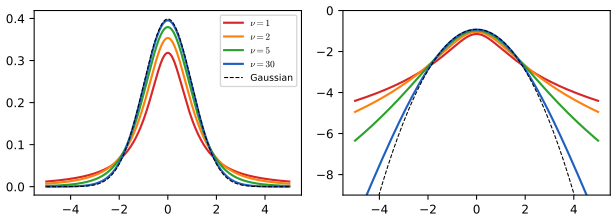
fig_2_S2. Download: PDF · SVGRobust fits (Figure 2.16). Thirty draws from \(\N(0,1)\) are fitted with a Gaussian, a Student distribution with \(\nu=4\) (EM) and a Laplace distribution. On the clean data the three agree. Adding three outliers near 8 moves the Gaussian mean from \(-0.12\) to \(0.60\) and its standard deviation from 0.81 to 2.42; the Student location moves to \(-0.05\) with scale 0.94, and the Laplace location (the median) to \(0.04\). Large \(\nu\) destroys the robustness: for \(\nu=30\) the Student location is 0.42, close to the Gaussian's. The rule of thumb \(\nu=4\) works well in many problems.
See also (companion course): Section 2.3.7, Student's t-distribution.
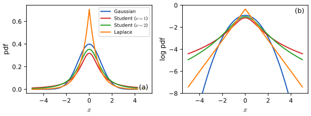
fig_2_15. Reproduces Murphy (2022), Figure 2.15. Download: PDF · SVG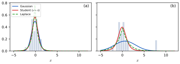
fig_2_16. Reproduces Murphy (2022), Figure 2.16. Download: PDF · SVG2.7.2 Cauchy distribution
p. 63 For \(\nu=1\) the Student is the Cauchy (Lorentz) distribution,
\[ \mathcal{C}(x\given\mu,\gamma)=\frac1{\gamma\pi}\Big[1+\Big(\frac{x-\mu}\gamma\Big)^2\Big]^{-1},\qquad\mathcal{C}_+(x\given\gamma)=\frac2{\pi\gamma}\Big[1+\Big(\frac x\gamma\Big)^2\Big]^{-1}\ (x\ge0) \tag{2.132, 2.133} \]where \(\mathcal{C}_+\) is the half-Cauchy (a heavy-tailed prior on positive scales with finite density at 0).
Result 2.13 (Cauchy and Laplace) pp. 63, (2.132)–(2.135)
(i) The standard Cauchy has cdf \(\frac12+\frac1\pi\arctan x\), so its central 95% interval is \(\pm\tan(0.475\pi)=\pm12.706\) (against \(\pm1.96\) for the standard normal). (ii) The Cauchy mean does not exist, and the mean of \(N\) iid standard Cauchy variables is again standard Cauchy: averaging does not help. (iii) The Laplace density \[ \mathrm{Laplace}(y\given\mu,b)=\frac1{2b}e^{-|y-\mu|/b} \] (2.134) has mean \(\mu\), mode \(\mu\) and variance \(2b^2\) (2.135); the maximum-likelihood fit is the sample median and the mean absolute deviation about it.
Proof
(i) \[ \int_{-\infty}^x\frac{\d t}{\pi(1+t^2)}=\frac1\pi(\arctan x+\frac\pi2); \] setting it to \(0.975\) gives \(x=\tan(0.475\pi)=12.706\). (ii) \[ \int_0^M\frac{x\,\d x}{\pi(1+x^2)}=\frac1{2\pi}\log(1+M^2)\to\infty \]: the positive and negative parts of \(\E[X]\) are both infinite, so the mean is undefined (the principal value 0 is not a mean). The characteristic function is \(\E[e^{itX}]=e^{-|t|}\); that of the average of \(N\) independent copies is \((e^{-|t|/N})^N=e^{-|t|}\), the same, so by uniqueness of characteristic functions the average is standard Cauchy. This is why the law of large numbers fails for heavy tails. (iii) By symmetry the mean and median are \(\mu\); \(\int\frac1{2b}e^{-|u|/b}\d u=1\); \[ \var=\int u^2\frac1{2b}e^{-|u|/b}\d u=\frac1b\int_0^\infty u^2e^{-u/b}\d u=\frac1b\cdot2b^3=2b^2. \] The log-likelihood of \(N\) points is \(-N\log2b-\frac1b\sum_n|y_n-\mu|\); the sum of absolute deviations is minimised by the median, and the maximum over \(b\) is at \(\hat b=\frac1N\sum_n|y_n-\hat\mu|\). The Laplace with \(b=1/\sqrt2\) has variance 1. ∎
2.7.3 Laplace distribution
p. 63 The Laplace (double-sided exponential) density \(\frac1{2b}e^{-|y-\mu|/b}\) has two parameters, a location \(\mu\) and a scale \(b>0\), and the properties of Result 2.13(iii). It is the basis of the lasso (Section 11.4) and robust regression (Section 11.6.1); its log density is a concave function (a negative absolute value), while the Student's is not log-concave for any \(\nu\) (the second derivative of \(-\frac{\nu+1}2\log(1+z^2/\nu)\) is positive for large \(|z|\)). The Student has a larger tail mass and the Laplace is a compromise between the two.
2.7.4 Beta distribution
pp. 63–64 The beta distribution has support \([0,1]\):
\[ \mathrm{Beta}(x\given a,b)=\frac1{B(a,b)}x^{a-1}(1-x)^{b-1},\qquad B(a,b)=\frac{\Gamma(a)\Gamma(b)}{\Gamma(a+b)},\quad\Gamma(a)=\int_0^\infty x^{a-1}e^{-x}\,\d x \tag{2.136--2.138} \]for \(a,b>0\). For \(a=b=1\) it is uniform; for \(a,b<1\) it is U-shaped with spikes at 0 and 1; for \(a,b>1\) it is unimodal.
Result 2.14 (the beta function and the beta moments; Exercise 2.8) p. 64, (2.137), (2.139), (2.188)–(2.190)
(i) \[ \int_0^1x^{a-1}(1-x)^{b-1}\d x=\Gamma(a)\Gamma(b)/\Gamma(a+b), \] so (2.136) is a density. (ii) For \(\theta\sim\mathrm{Beta}(a,b)\), \[ \E[\theta^k]=\dfrac{B(a+k,b)}{B(a,b)}=\prod_{j=0}^{k-1}\dfrac{a+j}{a+b+j}, \] hence
\[ \E[\theta]=\frac a{a+b},\qquad\var[\theta]=\frac{ab}{(a+b)^2(a+b+1)},\qquad \mathrm{mode}=\frac{a-1}{a+b-2}\ (a,b>1). \](iii) If \(a<1,b\ge1\) the density is unbounded at 0 and the mode is 0; if \(a\ge1,b<1\) the mode is 1.
Proof
(i) \[ \Gamma(a)\Gamma(b)=\int_0^\infty\!\!\int_0^\infty u^{a-1}v^{b-1}e^{-u-v}\d u\,\d v. \] Substitute \(u=st\), \(v=s(1-t)\) with \(s\in(0,\infty)\), \(t\in(0,1)\); the Jacobian is \[ \big|\det\left(\begin{smallmatrix}t&s\\1-t&-s\end{smallmatrix}\right)\big|=s. \] The integral becomes \[ \int_0^\infty s^{a+b-1}e^{-s}\d s\int_0^1t^{a-1}(1-t)^{b-1}\d t=\Gamma(a+b)B^*(a,b), \] where \(B^*\) is the beta integral, so \(B^*=\Gamma(a)\Gamma(b)/\Gamma(a+b)\). (ii) \[ \E[\theta^k]=\frac1{B(a,b)}\int\theta^{a+k-1}(1-\theta)^{b-1}=B(a+k,b)/B(a,b)=\dfrac{\Gamma(a+k)\Gamma(a+b)}{\Gamma(a)\Gamma(a+b+k)}, \] and \(\Gamma(x+1)=x\Gamma(x)\) turns the ratios into the product. Then \(\E[\theta]=\frac a{a+b}\), \[ \E[\theta^2]=\frac{a(a+1)}{(a+b)(a+b+1)}, \] and \[ \var=\E[\theta^2]-\E[\theta]^2=\frac{a}{a+b}\Big[\frac{a+1}{a+b+1}-\frac a{a+b}\Big]=\frac{ab}{(a+b)^2(a+b+1)}. \] (iii) \[ \frac{\d}{\d x}\log p=\frac{a-1}x-\frac{b-1}{1-x}=0 \] gives \(x=\frac{a-1}{a+b-2}\), a maximum when \(a,b>1\); if \(a<1\) the factor \(x^{a-1}\) blows up at 0, and similarly for \(b<1\) at 1. ∎
2.7.5 Gamma distribution
pp. 64–65 The gamma distribution on \(x>0\) with shape \(a\) and rate \(b\) (or scale \(s=1/b\)) is
\[ \mathrm{Ga}(x\given\text{shape}=a,\text{rate}=b)=\frac{b^a}{\Gamma(a)}x^{a-1}e^{-xb},\qquad\text{mean}=\frac ab,\ \ \text{mode}=\max\Big(\frac{a-1}b,0\Big),\ \ \var=\frac a{b^2}. \tag{2.140--2.142} \]Special cases: the exponential \[ \mathrm{Expon}(x\given\lambda)=\mathrm{Ga}(x\given1,\lambda) \] (2.143), the waiting time between events of a Poisson process of rate \(\lambda\); the chi-squared \[ \chi^2_\nu=\mathrm{Ga}(\frac\nu2,\frac12) \] (2.144), the law of \(\sum_{i=1}^\nu Z_i^2\), \(Z_i\sim\N(0,1)\); and the inverse gamma (2.145) with mean \(b/(a-1)\) (\(a>1\)), mode \(b/(a+1)\), variance \(b^2/((a-1)^2(a-2))\) (\(a>2\)) (2.146).
Result 2.15 (gamma moments, chi-squared, inverse gamma; Exercise 2.7) pp. 64–65, (2.140)–(2.146), (2.145)
(i) For \(X\sim\mathrm{Ga}(a,b)\) and any real \(k>-a\), \[ \E[X^k]=\dfrac{\Gamma(a+k)}{\Gamma(a)b^k}. \] In particular \(\E[X]=a/b\), \(\var[X]=a/b^2\), \(\E[1/X]=b/(a-1)\) for \(a>1\). (ii) If \(Z\sim\N(0,1)\) then \[ Z^2\sim\mathrm{Ga}(\frac12,\frac12); \] gamma variables with the same rate add their shapes, so the sum of \(\nu\) independent squared standard normals is \[ \mathrm{Ga}(\frac\nu2,\frac12)=\chi^2_\nu. \] (iii) If \[ X\sim\mathrm{Ga}(\text{shape }a,\text{rate }b) \] and \(Y=1/X\) then \[ p_Y(y)=\dfrac{b^a}{\Gamma(a)}y^{-(a+1)}e^{-b/y}, \] the inverse gamma with shape \(a\) and scale \(b\), with the moments (2.146).
Proof
(i) \[ \E[X^k]=\frac{b^a}{\Gamma(a)}\int x^{a+k-1}e^{-bx}\d x=\frac{b^a}{\Gamma(a)}\cdot\frac{\Gamma(a+k)}{b^{a+k}} \] (substitute \(u=bx\)), which gives the mean, \(\E[X^2]=a(a+1)/b^2\) and variance \(a/b^2\), and \[ \E[1/X]=\Gamma(a-1)b/\Gamma(a)=b/(a-1). \] The mode of \(x^{a-1}e^{-bx}\) is where \(\frac{a-1}x=b\), i.e. \(x=(a-1)/b\), if \(a>1\), else 0. (ii) By the change of variables of Result 2.16 with \(w=z^2\) (two branches \(z=\pm\sqrt w\)), \[ p(w)=2\cdot\phi(\sqrt w)\cdot\frac1{2\sqrt w}=\frac1{\sqrt{2\pi}}w^{-1/2}e^{-w/2}=\mathrm{Ga}(w\given\frac12,\frac12) \] since \(\Gamma(\frac12)=\sqrt\pi\). The moment generating function of \(\mathrm{Ga}(a,b)\) is \((1-t/b)^{-a}\) for \(t<b\) (Part (i) with the integral \(\int x^{a-1}e^{-(b-t)x}\)), so the product of independent ones with the same \(b\) is \((1-t/b)^{-\sum a_i}\): shapes add. (iii) \(g(y)=1/y\) has \(|g'(y)|=1/y^2\), so by (2.155) \[ p_Y(y)=\mathrm{Ga}(1/y\given a,b)/y^2=\frac{b^a}{\Gamma(a)}y^{-(a-1)}e^{-b/y}y^{-2}, \] the stated density. Its moments come from \[ \E[Y^k]=\E[X^{-k}]=\Gamma(a-k)b^k/\Gamma(a) \]: mean \(b/(a-1)\), \(\E[Y^2]=b^2/((a-1)(a-2))\), variance \(b^2/((a-1)^2(a-2))\); the mode solves \[ \frac{\d}{\d y}[-(a+1)\log y-b/y]=0, \] i.e. \(y=b/(a+1)\). ∎
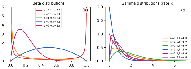
fig_2_17. Reproduces Murphy (2022), Figure 2.17. Download: PDF · SVG2.7.6 Empirical distribution
pp. 65–66 For samples \[ \mathcal{D}=\{x^{(1)},\dots,x^{(N)}\} \] the empirical distribution puts mass \(1/N\) on each:
\[ \hat p_N(x)=\frac1N\sum_{n=1}^N\delta_{x^{(n)}}(x),\qquad\hat P_N(x)=\frac1N\sum_{n=1}^N\mathbb{I}\big(x^{(n)}\le x\big)=\frac1N\sum_nu_{x^{(n)}}(x), \tag{2.147, 2.148} \]where \(u_y(x)=\mathbb{I}(x\ge y)\) is the step function (2.149): a staircase with jumps \(1/N\) (Figure 2.18). For fixed \(x\), \[ N\hat P_N(x)\sim\mathrm{Bin}(N,P(x)) \] when the samples are iid with cdf \(P\), so \(\E[\hat P_N(x)]=P(x)\) and \(\var[\hat P_N(x)]=P(x)(1-P(x))/N\) (Result 2.5): the empirical cdf is unbiased and consistent. The Dvoretzky–Kiefer–Wolfowitz inequality strengthens this to a uniform statement, \[ \Pr(\sup_x|\hat P_N-P|>\varepsilon)\le2e^{-2N\varepsilon^2}, \] proved with a demonstration in All of Statistics, Chapter 7. Replacing each spike by a smooth bump gives the kernel density estimate of Section 16.3.
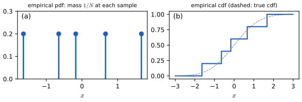
fig_2_18. Reproduces Murphy (2022), Figure 2.18. Download: PDF · SVG2.8 Transformations of random variables *
p. 66 If \(x\sim p(\cdot)\) and \(y=f(x)\) is a deterministic transformation, what is the distribution of \(y\)?
2.8.1 Discrete case
Sum the mass of all the \(x\) that map to \(y\): \(p_Y(y)=\sum_{x:f(x)=y}p_X(x)\) (2.150). For \(f(X)=\mathbb{I}(X\text{ even})\) and \(X\) uniform on \(\{1,\dots,10\}\), \(p_Y(1)=p_Y(0)=0.5\); \(f\) is many-to-one.
2.8.2 Continuous case
p. 67 One cannot sum densities, so work with cdfs: \[ P_Y(y)=\Pr(f(X)\le y)=\Pr(X\in\{x:f(x)\le y\}) \] (2.151). If \(f\) is invertible the pdf follows by differentiating; otherwise use numerical integration or Monte Carlo. A worked non-invertible example is \(y=x^2\) with \(x\sim\mathrm{Unif}(-1,1)\): \[ P_Y(y)=\Pr(-\sqrt y\le X\le\sqrt y)=\sqrt y, \] so \(p_Y(y)=\dfrac1{2\sqrt y}\) on \((0,1)\), with an integrable spike at 0 (Figure 2.24).
2.8.3 Invertible transformations (bijections)
2.8.3.1 Change of variables: scalar case
Result 2.16 (change of variables, scalar and multivariate) pp. 67–69, (2.152)–(2.161)
(a) Let \(X\) have pdf \(p_X\) and \(f:\mathbb{R}\to\mathbb{R}\) be strictly monotone and differentiable with inverse \(g=f^{-1}\) (differentiable). Then \(Y=f(X)\) has pdf \(p_Y(y)=p_X(g(y))\,|g'(y)|\) (2.155). (b) For a differentiable bijection \(f:\mathbb{R}^n\to\mathbb{R}^n\) with inverse \(g\) and Jacobian matrix \[ \mathbf{J}_g(\mathbf{y})=\partial g/\partial\mathbf{y}^\T, \] \[ p_Y(\mathbf{y})=p_X(g(\mathbf{y}))\,|\det\mathbf{J}_g(\mathbf{y})| \] (2.156). (c) If \(g\) is not monotone but each \(y\) has finitely many preimages \(x_k(y)\), \[ p_Y(y)=\sum_kp_X(x_k(y))\,|x_k'(y)|. \]
Proof
(a) If \(f\) is increasing, \[ P_Y(y)=\Pr(f(X)\le y)=\Pr(X\le g(y))=P_X(g(y)) \] (2.153); differentiating, \(p_Y(y)=p_X(g(y))\,g'(y)\) (2.154), and \(g'>0\). If \(f\) is decreasing, \(f(X)\le y\iff X\ge g(y)\), so \(P_Y(y)=1-P_X(g(y))\) and \(p_Y(y)=-p_X(g(y))g'(y)\), with \(g'<0\). In both cases the density is multiplied by \(|g'|\), which is (2.155). Heuristically, probability mass is preserved: \(p_X(x)|\d x|=p_Y(y)|\d y|\) (Figure 2.19).
(b) For a measurable set \(B\), \[ \Pr(Y\in B)=\Pr(X\in g(B))=\int_{g(B)}p_X(\mathbf{x})\,\d\mathbf{x}. \] The change-of-variables theorem for integrals under the diffeomorphism \(\mathbf{x}=g(\mathbf{y})\) gives \[ \int_Bp_X(g(\mathbf{y}))|\det\mathbf{J}_g(\mathbf{y})|\,\d\mathbf{y}. \] Since this holds for every \(B\), the integrand is the density of \(Y\) (almost everywhere). The determinant is the local volume scale factor of \(g\): a unit cube at \(\mathbf{y}\) maps to a parallelepiped of volume \(|\det\mathbf{J}_g|\). (c) Apply (a) on each interval of monotonicity (the preimage of \(\{y\le t\}\) is a union of intervals) and add. ∎
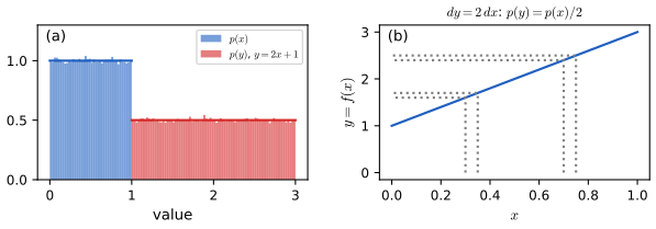
fig_2_19. Reproduces Murphy (2022), Figure 2.19 (the book's panel (b) is a sketch of the local mapping). Download: PDF · SVG2.8.3.2 Change of variables: multivariate case
pp. 68–69 For the affine map \[ f(\mathbf{x})=\mathbf{A}\mathbf{x}+\mathbf{b}, \] \[ g(\mathbf{y})=\mathbf{A}^{-1}(\mathbf{y}-\mathbf{b}), \] \(\mathbf{J}_g=\mathbf{A}^{-1}\) and \[ p_Y(\mathbf{y})=p_X(\mathbf{A}^{-1}(\mathbf{y}-\mathbf{b}))/|\det\mathbf{A}| \]: the unit square maps to a parallelogram of area \(|\det\mathbf{A}|\) (Figure 2.20, with \(\det\mathbf{A}=ad-bc\)), and a translation changes no areas. For polar coordinates \[ g(r,\theta)=(r\cos\theta,r\sin\theta), \]
\[ \mathbf{J}_g=\begin{pmatrix}\cos\theta&-r\sin\theta\\\sin\theta&r\cos\theta\end{pmatrix},\qquad|\det\mathbf{J}_g|=|r\cos^2\theta+r\sin^2\theta|=|r|, \tag{2.157, 2.158} \] \[ p_{r,\theta}(r,\theta)=p_{x_1,x_2}(r\cos\theta,r\sin\theta)\,r. \tag{2.159} \]Geometrically the shaded patch of Figure 2.21 has area \(r\,\d r\,\d\theta\) (exactly \[ \frac12[(r+\d r)^2-r^2]\d\theta=(r+\frac{\d r}2)\d r\,\d\theta \]), so \[ p_{r,\theta}\,\d r\,\d\theta=p_{x_1,x_2}\,r\,\d r\,\d\theta \] (2.160)–(2.161). This is the step that evaluates the Gaussian integral in Result 2.9 and, in Exercise 3.6 of the book, the multivariate normalising constant.
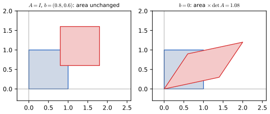
fig_2_20. Reproduces the idea of Murphy (2022), Figure 2.20, with a different matrix. Download: PDF · SVG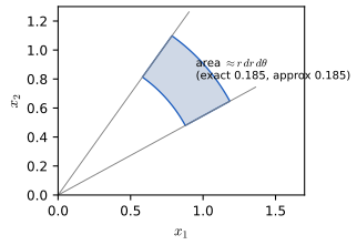
fig_2_21. Reproduces Murphy (2022), Figure 2.21. Download: PDF · SVG2.8.4 Moments of a linear transformation
pp. 69–70 For \[ \mathbf{y}=\mathbf{A}\mathbf{x}+\mathbf{b} \] with \[ \mathbb{E}[\mathbf{x}]=\boldsymbol\mu \] and \[ \mathrm{Cov}[\mathbf{x}]=\boldsymbol\Sigma \]:
\[ \E[\mathbf{y}]=\mathbf{A}\boldsymbol\mu+\mathbf{b},\qquad\E[\mathbf{a}^\T\mathbf{x}+b]=\mathbf{a}^\T\boldsymbol\mu+b,\qquad\mathrm{Cov}[\mathbf{y}]=\mathbf{A}\boldsymbol\Sigma\mathbf{A}^\T,\qquad\var[\mathbf{a}^\T\mathbf{x}+b]=\mathbf{a}^\T\boldsymbol\Sigma\mathbf{a}. \tag{2.162, 2.163, 2.164, 2.165} \]Result 2.17 (moments of an affine map; the variance of a sum) p. 70, (2.162)–(2.167)
The formulas (2.162)–(2.165) hold for every distribution with finite second moments, not only the Gaussian; in particular \[ \var[x_1+x_2]=\Sigma_{11}+\Sigma_{22}+2\Sigma_{12}=\var[x_1]+\var[x_2]+2\cov[x_1,x_2] \] (2.166, 2.167), and \(\mathrm{Cov}[\mathbf{y}]\) is positive semi-definite.
Proof (the exercise the book leaves)
Linearity of expectation (Filling the gap 2.5) applied entrywise gives (2.162): \(\E[y_i]=\sum_jA_{ij}\E[x_j]+b_i\). Put \[ \tilde{\mathbf{y}}=\mathbf{y}-\E[\mathbf{y}]=\mathbf{A}(\mathbf{x}-\boldsymbol\mu). \] Then \[ \mathrm{Cov}[\mathbf{y}]=\E[\tilde{\mathbf{y}}\tilde{\mathbf{y}}^\T]=\E[\mathbf{A}(\mathbf{x}-\boldsymbol\mu)(\mathbf{x}-\boldsymbol\mu)^\T\mathbf{A}^\T]=\mathbf{A}\boldsymbol\Sigma\mathbf{A}^\T, \] since \(\mathbf{A}\) is constant. A scalar map is the case where \(\mathbf{A}=\mathbf{a}^\T\) is a row vector. Taking \(\mathbf{a}=(1,1)^\T\), \[ \mathbf{a}^\T\boldsymbol\Sigma\mathbf{a}=\Sigma_{11}+\Sigma_{12}+\Sigma_{21}+\Sigma_{22}. \] For any \(\mathbf{v}\), \[ \mathbf{v}^\T\mathbf{A}\boldsymbol\Sigma\mathbf{A}^\T\mathbf{v}=\var[(\mathbf{A}^\T\mathbf{v})^\T\mathbf{x}]\ge0. \] The book's remark that a distribution other than the Gaussian is not determined by its mean and covariance means (2.162)–(2.165) give only the first two moments of \(\mathbf{y}\), not its law. ∎
2.8.5 The convolution theorem
pp. 70–72 Let \(y=x_1+x_2\) with independent \(x_1\), \(x_2\). In the discrete case \(p(y=j)=\sum_kp(x_1=k)p(x_2=j-k)\) (2.168). In the continuous case, integrating the joint density over \(x_1+x_2\le y^*\),
\[ P_y(y^*)=\int_{-\infty}^\infty p_1(x_1)\Big[\int_{-\infty}^{y^*-x_1}p_2(x_2)\,\d x_2\Big]\d x_1\ \ (2.169),\qquad p(y)=\int p_1(x_1)\,p_2(y-x_1)\,\d x_1=(p_1\circledast p_2)(y). \tag{2.170, 2.172} \]Result 2.18 (convolution theorem; sums of Gaussians; Exercise 2.4) pp. 70–72, (2.168)–(2.176)
(a) The density of a sum of independent variables is the convolution (2.170); for finite sequences it is the "flip and drag" product of Table 2.4, e.g. \[ [1,2,3,4]\circledast[5,6,7]=[5,16,34,52,45,28]. \] (b) If \(x_1\sim\N(\mu_1,\sigma_1^2)\) and \(x_2\sim\N(\mu_2,\sigma_2^2)\) are independent, \[ y=x_1+x_2\sim\N(\mu_1+\mu_2,\sigma_1^2+\sigma_2^2) \] (2.176). (c) The distribution of the sum of two dice is the convolution of two uniforms on \(\{1,\dots,6\}\): \(p(y)=(6-|y-7|)/36\) for \(y=2,\dots,12\) (2.173)–(2.175).
Proof
(a) Independence factorises the joint density, so \[ P_y(y^*)=\iint_{x_1+x_2\le y^*}p_1(x_1)p_2(x_2)\,\d x_1\d x_2, \] which is (2.169) by Fubini. Differentiate in \(y^*\) with Leibniz's rule (2.171): the inner integral has upper limit \(y^*-x_1\) with derivative 1 in \(y^*\), and no dependence of the lower limit, giving \[ p(y^*)=\int p_1(x_1)p_2(y^*-x_1)\,\d x_1. \] (b) Use the density of \(x_1+x_2\) and complete the square. With \(m_i=\mu_i\), \(v_i=\sigma_i^2\), and \(u=y-m_1-m_2\), \(t=x_1-m_1\), the exponent of the integrand is \[ -\frac{t^2}{2v_1}-\frac{(u-t)^2}{2v_2}. \] Expanding, \[ -\frac12\big[(\tfrac1{v_1}+\tfrac1{v_2})t^2-\tfrac{2u}{v_2}t+\tfrac{u^2}{v_2}\big]=-\frac{v_1+v_2}{2v_1v_2}\big(t-\frac{v_1u}{v_1+v_2}\big)^2-\frac{u^2}{2(v_1+v_2)}. \] The integral over \(t\) of the first term is the Gaussian integral \(\sqrt{2\pi v_1v_2/(v_1+v_2)}\) (Result 2.9), so \[ p(y)=\frac1{2\pi\sqrt{v_1v_2}}\sqrt{\frac{2\pi v_1v_2}{v_1+v_2}}e^{-u^2/2(v_1+v_2)}=\N(y\given m_1+m_2,v_1+v_2). \] Alternatively, the characteristic function of the sum is the product of those of the summands, \[ e^{it\mu_1-\sigma_1^2t^2/2}e^{it\mu_2-\sigma_2^2t^2/2}, \] the characteristic function of the stated Gaussian. (c) With \(p_1=p_2=1/6\) on \(\{1,\dots,6\}\), \[ p(y)=\frac1{36}\#\{(k,y-k):1\le k,y-k\le6\}, \] which is \(\min(y-1,13-y)/36\). A numerical convolution on a grid with spacing 0.01 reproduces (b) to \(10^{-6}\). ∎
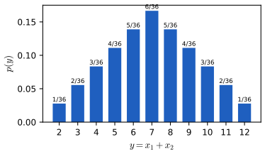
fig_2_22. Reproduces Murphy (2022), Figure 2.22. Download: PDF · SVG2.8.6 Central limit theorem
pp. 72 Let \(X_1,\dots,X_N\) be iid with mean \(\mu\) and variance \(\sigma^2\), \(S_N=\sum_nX_n\) and \(\bar X=S_N/N\). The central limit theorem (CLT) says that
\[ Z_N\triangleq\frac{S_N-N\mu}{\sigma\sqrt N}=\frac{\bar X-\mu}{\sigma/\sqrt N}\ \xrightarrow{d}\ \N(0,1),\qquad\text{loosely}\ \ p(S_N=u)\approx\frac1{\sqrt{2\pi N\sigma^2}}\exp\Big(-\frac{(u-N\mu)^2}{2N\sigma^2}\Big). \tag{2.177, 2.178} \]Result 2.19 (the central limit theorem, with proof and rate; the caveat on (2.177)) p. 72, (2.177)–(2.178)
(a) If \(X_n\) are iid with finite mean \(\mu\) and variance \(\sigma^2>0\), then \(\Pr(Z_N\le z)\to\Phi(z)\) for every \(z\). (b) If in addition \(\rho=\E|X-\mu|^3<\infty\), then \[ \sup_z|\Pr(Z_N\le z)-\Phi(z)|\le C\rho/(\sigma^3\sqrt N) \] with an absolute constant \(C\le0.4748\) (Berry–Esseen). (c) The leading error for a non-lattice distribution with skewness \(\gamma=\E(X-\mu)^3/\sigma^3\) is \[ \Pr(Z_N\le z)-\Phi(z)=-\dfrac{\gamma}{6\sqrt N}(z^2-1)\phi(z)+o(N^{-1/2}), \] so \[ \sup_z|\cdot|\approx0.0665\,|\gamma|/\sqrt N. \] (d) Convergence of the densities to the normal curve, the literal reading of (2.177), requires an extra assumption (for example that \(X\) has a bounded density), and for a lattice variable (dice, coin counts) the statement is about the pmf times the lattice spacing.
Proof of (a) (assuming a finite moment generating function; the general case uses characteristic functions)
Standardise: \(Y_n=(X_n-\mu)/\sigma\) have mean 0, variance 1, and \(Z_N=N^{-1/2}\sum_nY_n\). Suppose \(M(t)=\E e^{tY}\) is finite near 0, with \(M(0)=1\), \(M'(0)=0\), \(M''(0)=1\); Taylor's theorem gives \(M(t)=1+\tfrac12t^2+o(t^2)\). By independence the mgf of \(Z_N\) is
\[ \E e^{tZ_N}=\Big[M\Big(\frac t{\sqrt N}\Big)\Big]^N=\Big[1+\frac{t^2}{2N}+o\Big(\frac1N\Big)\Big]^N\ \longrightarrow\ e^{t^2/2}\qquad(N\to\infty), \]using \((1+u_N/N)^N\to e^{u}\) when \(u_N\to u\). The limit is the mgf of \(\N(0,1)\), and convergence of mgfs in a neighbourhood of 0 implies convergence in distribution (Curtiss). For a general proof replace \(e^{tY}\) by \(e^{itY}\), whose expectation always exists: \(\varphi(t)=1-\tfrac12t^2+o(t^2)\) needs only a finite variance, and Lévy's continuity theorem gives the conclusion; a full proof is in All of Statistics, Section 5.7.2.
(c) Heuristic rate. Write the cumulant expansion \[ \log M(t)=\tfrac12t^2+\tfrac16\gamma t^3+O(t^4). \] Then \[ \log\E e^{tZ_N}=N\log M(t/\sqrt N)=\tfrac12t^2+\tfrac{\gamma}{6\sqrt N}t^3+O(1/N), \] so \[ \E e^{tZ_N}\approx e^{t^2/2}\big(1+\frac\gamma{6\sqrt N}t^3\big). \] Inverting, since \(\phi^{(k)}\) has mgf \((-t)^ke^{t^2/2}\) (integrate by parts \(k\) times), \(t^3e^{t^2/2}\) corresponds to \(-\phi'''(z)=(z^3-3z)\phi(z)\), so the density of \(Z_N\) is \[ \phi(z)\big[1+\frac{\gamma}{6\sqrt N}(z^3-3z)\big] \] and, integrating, the cdf is \[ \Phi(z)-\frac\gamma{6\sqrt N}(z^2-1)\phi(z) \] (the Edgeworth expansion, Feller 1971). The maximum of \(|(z^2-1)\phi(z)|\) is at \(z=0\), with value \(\phi(0)=0.3989\), giving \(0.3989/6=0.0665\). For the \(\mathrm{Beta}(1,5)\) of the book's Figure 2.23, \(\gamma=1.183\), so the predicted distance is \(0.0787/\sqrt N\); numerically (exact grid convolutions) the distances at \(N=1,2,5,10,30\) are \[ 0.114,\,0.065,\,0.037,\,0.0255,\,0.0145, \] and \(\sqrt N\times\) distance tends to \(0.079\). For the exponential (\(\gamma=2\)) the constant is \(0.133\), as in the demonstration below. ∎
(d) The cdf converging does not make the pdf converge. A sum of \(N\) Bernoulli variables is supported on the integers, so its distribution has no density at all, and the "density" in (2.177) is only a good approximation to the pmf, \[ \Pr(S_N=k)\approx\N(k\given N\mu,N\sigma^2) \] (the local limit theorem, Gnedenko 1948), when the lattice spacing 1 is small compared with \(\sigma\sqrt N\). With a bounded density for \(X\) the densities do converge. ∎
The book's example is the mean of \(N\) draws from \(\mathrm{Beta}(1,5)\), whose histogram over \(10{,}000\) replications is skewed for \(N=1\) and already close to bell-shaped at \(N=5\) (Figure 2.23). The interactive demonstration builds the exact density of the sum by repeated convolution, shows the standardised density against the Gaussian, the distribution-function gap and the decay of the Kolmogorov distance with \(N\), for four base distributions.
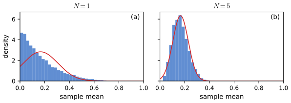
fig_2_23. Reproduces Murphy (2022), Figure 2.23. Download: PDF · SVG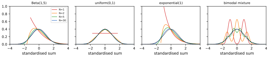
fig_2_S1. Download: PDF · SVGSee also (companion courses): All of Statistics, Section 5.4 and its Berry–Esseen demo; the first-year central limit theorem demo.
The CLT also explains the Gaussian two-dice shape of Figure 2.22 and is the reason a Gaussian is a good default model of measurement noise (Section 2.6.4); for heavy-tailed summands with infinite variance (Cauchy, Result 2.13) it fails and the sums converge to a stable law instead.
2.8.7 Monte Carlo approximation
p. 73 When the distribution of \(y=f(x)\) is hard to derive, draw \(x^{(1)},\dots,x^{(N_s)}\sim p_X\), set \(y_s=f(x^{(s)})\) and use the empirical distribution \[ p_S(y)=\frac1{N_s}\sum_s\delta(y-y_s) \] (2.179).
Result 2.20 (Monte Carlo is unbiased and converges at the rate \(1/\sqrt{N_s}\)) p. 73, (2.179)
For any \(h\) with \(\E|h(Y)|<\infty\), \(\hat I=\frac1{N_s}\sum_sh(y_s)\) satisfies \(\E[\hat I]=\E[h(Y)]\) and, if \(\var[h(Y)]=\tau^2<\infty\), \(\var[\hat I]=\tau^2/N_s\); moreover \(\hat I\to\E[h(Y)]\) almost surely (law of large numbers) and \[ \sqrt{N_s}(\hat I-\E h(Y))/\tau\xrightarrow{d}\N(0,1) \] (Result 2.19). In particular the Monte Carlo cdf \[ \hat P_{N_s}(t)=\frac1{N_s}\sum_s\mathbb{I}(y_s\le t) \] has standard error \[ \sqrt{P(t)(1-P(t))/N_s}\le\frac1{2\sqrt{N_s}}. \]
Proof
Linearity gives \(\E\hat I=\E h(Y)\); independence and (2.34) with (2.33) give \(\var\hat I=N_s\cdot\tau^2/N_s^2\). The almost-sure and distributional statements are the strong law and the CLT for the iid sequence \(h(y_s)\). The cdf is the case \(h=\mathbb{I}(\cdot\le t)\), a Bernoulli variable with variance \(P(1-P)\le\frac14\) (Result 2.5). Halving the error costs four times as many samples, whatever the dimension: this dimension-free rate is why Monte Carlo is the default tool in high dimensions. ∎
For \(x\sim\mathrm{Unif}(-1,1)\), \(y=x^2\), the exact density is \(1/(2\sqrt y)\) (Section 2.8.2); \(N_s=5000\) samples already give a histogram close to it except near the spike at \(y=0\), where the density is unbounded and any finite histogram bin underestimates the peak (Figure 2.24).
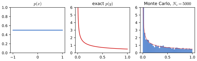
fig_2_24. Reproduces Murphy (2022), Figure 2.24. Download: PDF · SVGExercises
The twelve exercises of Section 2.9, restated, with worked solutions. (★ marks the book's starred exercises.) Computations use the code of the Python module.
Exercise 2.1 (conditional independence, ★). A variable \(H\in\{1,\dots,K\}\) has observed evidence values \(e_1\), \(e_2\) of two other variables \(E_1\), \(E_2\); we want the vector \(\mathbf{P}(H\given e_1,e_2)\). Which of these sets of numbers suffice: (i) \[ P(e_1,e_2),P(H),P(e_1\given H),P(e_2\given H); \] (ii) \(P(e_1,e_2),P(H),P(e_1,e_2\given H)\); (iii) \(P(e_1\given H),P(e_2\given H),P(H)\)? (a) in general, (b) if \(E_1\indep E_2\given H\).
Solution
Bayes' rule: \[ P(H\given e_1,e_2)=P(e_1,e_2\given H)P(H)/P(e_1,e_2). \] (a) Only (ii) contains all three factors. Set (i) lacks \(P(e_1,e_2\given H)\): the two single-evidence likelihoods do not determine the joint likelihood unless \(E_1\) and \(E_2\) are conditionally independent (two joint tables with the same marginals give different posteriors). Set (iii) lacks both that and the normaliser. (b) With \(E_1\indep E_2\given H\) we have \[ P(e_1,e_2\given H)=P(e_1\given H)P(e_2\given H), \] so all three sets suffice: sets (i) and (ii) now contain everything, and for (iii) the normaliser is recovered from the sum rule, \[ P(e_1,e_2)=\sum_hP(h)P(e_1\given h)P(e_2\given h), \] or equivalently by normalising the vector \(P(H)P(e_1\given H)P(e_2\given H)\) to sum to one. Numerically (random tables with \(K=4\)) the posterior from (iii) equals the true posterior to \(10^{-16}\) under conditional independence. ∎
Exercise 2.2 (pairwise independence does not imply mutual independence). Show by a counterexample that random variables can be pairwise independent without being mutually independent.
Solution
Take \(X_1,X_2\) independent fair bits and \(X_3=X_1\oplus X_2\). Each of \((X_1,X_2)\), \((X_1,X_3)\), \((X_2,X_3)\) is uniform on \(\{0,1\}^2\) (for \((X_1,X_3)\): \(X_2=X_1\oplus X_3\) is determined and uniform, so each pair has probability \(\frac14\)), hence \[ p(x_i,x_j)=\tfrac12\cdot\tfrac12=p(x_i)p(x_j). \] But \(p(1,1,1)=0\) (since \(1\oplus1=0\)) whereas \(p(1)p(1)p(1)=\tfrac18\). The pairwise condition (2.180)–(2.181) holds, the mutual condition (2.183) fails (Result 2.1). We confirmed the nine pair probabilities and the zero by enumeration. ∎
Exercise 2.3 (conditional independence iff the joint factorises, ★). Prove that \(X\indep Y\given Z\) iff there are functions \(g\), \(h\) with \(p(x,y\given z)=g(x,z)h(y,z)\) for all \(x,y,z\) with \(p(z)>0\).
Solution
(⇒) Take \(g(x,z)=p(x\given z)\), \(h(y,z)=p(y\given z)\). (⇐) Suppose \(p(x,y\given z)=g(x,z)h(y,z)\). Marginalise: \[ p(x\given z)=\sum_yp(x,y\given z)=g(x,z)H(z) \] with \(H(z)=\sum_yh(y,z)\), and \(p(y\given z)=h(y,z)G(z)\) with \(G(z)=\sum_xg(x,z)\) (sums become integrals for continuous variables). Since \[ 1=\sum_{x,y}p(x,y\given z)=G(z)H(z), \]
\[ p(x\given z)p(y\given z)=g(x,z)h(y,z)G(z)H(z)=g(x,z)h(y,z)=p(x,y\given z). \]The factors need not be normalised, which is the practical use of the criterion: in a graphical model any factorisation \[ p(x,y,z)\propto\psi_1(x,z)\psi_2(y,z) \] implies \(X\indep Y\given Z\). ∎
Exercise 2.4 (convolution of two Gaussians is a Gaussian). Show \[ \N(x_1\given\mu_1,\sigma_1^2)\circledast\N(x_2\given\mu_2,\sigma_2^2)=\N(y\given\mu_1+\mu_2,\sigma_1^2+\sigma_2^2) \] for \(y=x_1+x_2\), independent.
Solution
This is Result 2.18(b), proved there by completing the square (and by characteristic functions). A numerical convolution of \(\N(1,1.5^2)\) and \(\N(-2,0.8^2)\) on a grid of spacing 0.01 matches \(\N(-1,1.5^2+0.8^2)\) to within \(10^{-6}\) everywhere. ∎
Exercise 2.5 (expected value of the minimum of two rvs, ★). \(X,Y\) are independent uniform on \([0,1]\). What is the expected location of the leftmost point?
Solution
\(M=\min(X,Y)\) exceeds \(t\) iff both do: \(\Pr(M>t)=(1-t)^2\) on \([0,1]\). For a non-negative variable \[ \E[M]=\int_0^1\Pr(M>t)\,\d t=\int_0^1(1-t)^2\d t=\tfrac13. \] Equivalently the density is \(p_M(t)=2(1-t)\) and \[ \E M=\int_0^1t\cdot2(1-t)\,\d t=1-\tfrac23=\tfrac13. \] By symmetry \(\E[\max]=\tfrac23\) and \(\E[M]+\E[\max]=\E[X+Y]=1\), consistent. A simulation of \(10^6\) pairs gives \(0.3333\). ∎
Exercise 2.6 (variance of a sum). Show \[ \var[X+Y]=\var[X]+\var[Y]+2\cov[X,Y]. \]
Solution
With means \(\mu_X,\mu_Y\): \[ \var[X+Y]=\E[((X-\mu_X)+(Y-\mu_Y))^2]=\E[(X-\mu_X)^2]+\E[(Y-\mu_Y)^2]+2\E[(X-\mu_X)(Y-\mu_Y)], \] by expanding the square and linearity; the three terms are \(\var[X]\), \(\var[Y]\) and \(2\cov[X,Y]\). The same follows from Result 2.17 with \(\mathbf{a}=(1,1)^\T\). ∎
Exercise 2.7 (deriving the inverse gamma density, ★). \(X\sim\mathrm{Ga}(a,b)\) (shape \(a\), rate \(b\)) and \(Y=1/X\). Derive the distribution of \(Y\).
Solution
\(y=1/x\) is a decreasing bijection of \((0,\infty)\) with inverse \(g(y)=1/y\), \(|g'(y)|=y^{-2}\). By (2.155), \[ p_Y(y)=\mathrm{Ga}(1/y\given a,b)\,y^{-2}=\dfrac{b^a}{\Gamma(a)}y^{-(a-1)}e^{-b/y}y^{-2}=\dfrac{b^a}{\Gamma(a)}y^{-(a+1)}e^{-b/y}, \] the inverse gamma \[ \mathrm{IG}(y\given\text{shape }a,\text{scale }b) \] of (2.145); the moments follow as in Result 2.15(iii). We checked numerically that the transformed density equals the stated formula and scipy's
invgammato \(10^{-10}\), and that the mean is \(b/(a-1)\) and the mode \(b/(a+1)\). ∎Exercise 2.8 (mean, mode, variance for the beta distribution). For \(\theta\sim\mathrm{Beta}(a,b)\) show \(\E\theta=\frac a{a+b}\), \[ \var\theta=\frac{ab}{(a+b)^2(a+b+1)}, \] mode \(\frac{a-1}{a+b-2}\).
Solution
Result 2.14(ii) and (iii) prove all three, using \[ B(a,b)=\Gamma(a)\Gamma(b)/\Gamma(a+b) \] and \(\Gamma(x+1)=x\Gamma(x)\); the mode needs \(a,b>1\). Numerically, for \((a,b)=(2,8),(3,2),(0.7,1.4)\) the integrals of \(x\,p\) and \((x-\bar x)^2p\) match the closed forms to \(10^{-3}\) and the pdf matches scipy to \(10^{-9}\). ∎
Exercise 2.9 (Bayes' rule for medical diagnosis, ★). A test for a disease that strikes one person in 10,000 is 99% accurate: \[ P(\text{positive}\given\text{disease})=0.99 \] and \[ P(\text{negative}\given\text{no disease})=0.99. \] You test positive. What is the probability you have the disease?
Solution
\[ P(D\given+)=\dfrac{0.99\times10^{-4}}{0.99\times10^{-4}+0.01\times(1-10^{-4})}=\dfrac{0.000099}{0.000099+0.009999}=0.0098, \] about \(1\%\). In a population of one million: 100 have the disease and 99 of them test positive; of the 999,900 healthy people, 9,999 test positive; so \(99/(99+9999)=0.0098\). A "99% accurate" test is overwhelmed by the rarity of the disease: the likelihood ratio is 99, but the prior odds are only \(10^{-4}\), giving posterior odds \(0.0099\). This is the demonstration's preset 3. ∎
Exercise 2.10 (legal reasoning). Blood with no innocent explanation is found at a crime scene; its type is present in 1% of the population. (a) The prosecutor argues: "there is a 1% chance the defendant would have this type if innocent, so a 99% chance he is guilty". What is wrong? (b) The defender argues: "the city has 800,000 people, so about 8,000 have this type; the evidence gives only a 1 in 8,000 chance of guilt and is irrelevant". What is wrong?
Solution
Let \(E\) = "defendant has the type", \(G\) = "guilty". (a) The prosecutor equates \(P(E\given\neg G)=0.01\) with \(1-P(G\given E)\): this transposes the conditional (the prosecutor's fallacy). Bayes' rule gives \[ P(G\given E)=\dfrac{P(E\given G)P(G)}{P(E\given G)P(G)+0.01(1-P(G))}, \] which depends on the prior \(P(G)\); the 1% is only the likelihood under innocence. (b) With a uniform prior over the 800,000 inhabitants, \(P(G)=1/800{,}000\) and \(P(E\given G)=1\), so \[ P(G\given E)=\dfrac{1/800{,}000}{1/800{,}000+0.01(1-1/800{,}000)}=\dfrac1{1+0.01\times799{,}999}=\dfrac1{8001}\approx\dfrac1{8000} \]: the defender's 1 in 8,000 is the right number, but not "irrelevant": the evidence multiplied the odds of guilt by 100 (from \(1.25\times10^{-6}\) to \(1.25\times10^{-4}\)). The error is to ignore that the posterior should be compared with the prior, and to forget the other evidence that made the defendant a suspect in the first place (the prior is not uniform over the city: it is conditioned on whatever led the police to him). The demonstration's preset 4 shows the numbers. ∎
Exercise 2.11 (probabilities are sensitive to the form of the question, ★). A neighbour has two children; gender is a fair coin flip, so one boy and one girl has probability \(\frac12\), two boys \(\frac14\), two girls \(\frac14\). (a) You ask whether he has any boys and he says yes. What is the probability that one child is a girl? (b) Instead you see one of his children run by and it is a boy. What is the probability that the other is a girl?
Solution
(a) The answer "yes" eliminates only the girl–girl case, leaving BB, BG, GB with probabilities \(\frac14\) each: \[ P(\text{one girl}\given\text{any boy})=\dfrac{2/4}{3/4}=\dfrac23. \] (b) Seeing a particular child is a boy: the child seen is equally likely to be either of the two. \(P(\text{see a boy}\given BB)=1\), \[ P(\ldots\given BG)=P(\ldots\given GB)=\frac12, \] \(P(\ldots\given GG)=0\). Then \[ P(\text{other is a girl}\given\text{saw a boy})=\dfrac{\frac14\cdot\frac12+\frac14\cdot\frac12}{\frac14\cdot1+\frac14\cdot\frac12+\frac14\cdot\frac12}=\dfrac{1/4}{1/2}=\dfrac12. \] The two cases differ in the likelihood of the observation, exactly as in the Monty Hall problem with a random host (Result 2.4(b)): in (a) the question "any boys?" has the same answer yes in BB, BG, GB; in (b) the act of seeing a boy is more likely when both children are boys. Enumeration confirms \(\frac23\) and \(\frac12\). ∎
▶ DemoThe form of the question: informed against random hostThe same data, different generating processes, different posteriors.Exercise 2.12 (normalisation constant for a 1D Gaussian). Show \[ Z=\int_{-\infty}^\infty\exp(-x^2/2\sigma^2)\,\d x=\sqrt{2\pi\sigma^2} \] by squaring and changing to polar coordinates.
Solution
Result 2.9(i): \[ Z^2=\int_0^{2\pi}\int_0^\infty r\,e^{-r^2/2\sigma^2}\d r\,\d\theta=2\pi\cdot\sigma^2, \] because \[ \int_0^\infty re^{-r^2/2\sigma^2}\d r=[-\sigma^2e^{-r^2/2\sigma^2}]_0^\infty=\sigma^2 \] (the hint's \(u=e^{-r^2/2\sigma^2}\), \(u'=-\sigma^{-2}re^{-r^2/2\sigma^2}\)). Hence \(Z=\sqrt{2\pi\sigma^2}\) (\(Z>0\)). A numerical quadrature of \(\int e^{-t^2/2}\) and of the double integral both give \(2\pi\) for \(Z^2\) to \(10^{-8}\). ∎
Demonstrations for this chapter
Each demonstration runs in the browser, with seeded random numbers so that a class sees the same pictures, and links back to these notes. The ▶ Demo boxes above open them already set to the case under discussion. Each page reproduces the Python code's numbers (the posteriors exactly, the Monte Carlo win rates within sampling error, the convolution distances to \(10^{-4}\) and the robust fits to \(10^{-6}\)).
| Demonstration | What it shows | Notes section |
|---|---|---|
| Bayes' rule for a diagnostic test (5 presets) | Prior, sensitivity and specificity to posterior; frequency table; repeated tests; posterior against prevalence | 2.3.1, Ex. 2.9, 2.10 |
| The Monty Hall problem (4 presets) | Simulated win rates of staying and switching with \(n\) doors, informed or random host, against the exact posterior | 2.3.2, Ex. 2.11 |
| Convolution and the central limit theorem (5 presets) | Exact density of the sum of \(N\) variables, distribution-function gap and Kolmogorov distance, with a histogram | 2.8.5, 2.8.6 |
| Heavy tails and robust fits (5 presets) | Gaussian, Student and Laplace fits with outliers; log densities; influence of one point | 2.7.1 |
The Python code that produces every figure of this page is code/ch02_probability_univariate.py (see the code index).
References
- Murphy, K. P. (2022). Probabilistic Machine Learning: An Introduction. MIT Press, Cambridge, MA. Chapter 2, pp. 33–76. probml.github.io/pml-book/book1.html.
- Anscombe, F. J. (1973). Graphs in statistical analysis. The American Statistician, 27(1), 17–21.
- Bishop, C. M. (2006). Pattern Recognition and Machine Learning. Springer, New York.
- Dvoretzky, A., Kiefer, J. and Wolfowitz, J. (1956). Asymptotic minimax character of the sample distribution function and of the classical multinomial estimator. Annals of Mathematical Statistics, 27(3), 642–669.
- Feller, W. (1971). An Introduction to Probability Theory and Its Applications, Volume II, 2nd edition. Wiley, New York.
- Gnedenko, B. V. (1948). On a local limit theorem of the theory of probability. Uspekhi Matematicheskikh Nauk, 3(3), 187–194.
- Jaynes, E. T. (2003). Probability Theory: The Logic of Science. Cambridge University Press.
- Matejka, J. and Fitzmaurice, G. (2017). Same stats, different graphs: generating datasets with varied appearance and identical statistics through simulated annealing. Proceedings of the CHI Conference on Human Factors in Computing Systems, 1290–1294.
- Shevtsova, I. G. (2011). On the absolute constants in the Berry–Esseen type inequalities for identically distributed summands. arXiv:1111.6554.
- Wasserman, L. (2004). All of Statistics. Springer, New York.
The numerical statements in the text (the identities for the sigmoid, softmax and log-sum-exp, the Bayes posteriors and Monty Hall probabilities, the moments of the Student, Laplace, beta and gamma distributions, the change-of-variables densities, the convolution of Gaussians, the Kolmogorov distances of the central limit theorem, and the fitted regressions and robust fits) were confirmed numerically.