Random Variables
A random variable attaches a number to each outcome of an experiment, and from then on we reason about the numbers rather than the outcomes. This chapter builds the vocabulary for doing that: the distribution function, which determines everything about a single random variable and can be recognised by three simple properties; mass functions and densities; the quantile function, which turns uniform random numbers into draws from any distribution; the standard families; joint, marginal and conditional distributions and what independence means for them; the multinomial and the multivariate normal; and the calculus of transformations, from the three-step cdf method and the Jacobian to the convolution formula for sums and the laws of the maximum and the minimum.
Ch. 1 Probability Ch. 2 Random variables Ch. 3 Expectation Ch. 4 Inequalities Ch. 5 Convergence Ch. 6 Models and inference Ch. 7 Estimating the CDF Ch. 8 Bootstrap Ch. 9 Parametric inference Ch. 10 Hypothesis testing Ch. 11 Bayesian inference Ch. 12 Decision theory Ch. 13 Regression Ch. 14 Multivariate models Ch. 15 Independence Ch. 16 Causal inference Ch. 17 Directed graphs Ch. 18 Undirected graphs Ch. 19 Log-linear models Ch. 20 Curve estimation Ch. 21 Orthogonal functions Ch. 22 Classification Ch. 23 Stochastic processes Ch. 24 Simulation
How to read these notes
They follow the book. Sections carry the book's numbers (2.1, 2.2, ...), and every displayed equation that the book numbers carries the book's own number, e.g. \((2.12)\). Theorems, lemmas and examples are referred to by the book's numbers (Theorem 2.8, Example 2.48); the definitions and results of these notes are numbered separately (Result 2.4), and each says which statement of the book it is.
Filling the gaps. The chapter states many facts without proof: that a cdf determines its distribution, the converse half of Theorem 2.8 ("uses some deep tools in analysis"), the binomial formula ("it can be shown"), the closure of the standard families under sums, the factorisation criteria for independence, the multinomial marginals, all of Theorems 2.43 and 2.44 on the multivariate normal, and the transformation formula (2.12). Every one is proved below, in the proof attached to its result or in an orange Filling the gap box, and the chapter's transformation recipe is extended to the Jacobian formula in several variables, the convolution formula and the laws of the maximum and minimum. Proofs start hidden: open one with its bar, or use the button below.
Figures and demonstrations. All six figures of the chapter are redrawn by the Python code, from the exact functions and regions; six supplementary figures (2.S1 to 2.S6) illustrate the examples and the computer exercises. The ▶ Demo boxes open an interactive demonstration already set to the case being discussed.
Main reference
L. Wasserman, All of Statistics: A Concise Course in Statistical Inference, Springer (2004), Chapter 2, pages 19–46 (book website, with the data sets and the author's errata: www.stat.cmu.edu/~larry/all-of-statistics). Section, equation, theorem, example and exercise numbers below refer to this book. Further reading is listed in the references.
The explanations, derivations, figures and code are my own; equations are cited by their numbers in the book.
Companion courses
Distributions and their transformations are the common ground of every course on this site. The overlapping material is:
- Sections 2.2–2.4 (densities, the standard families): Foundations of Deep Learning, Section 2.2 (probability densities) and Section 3.1 (Bernoulli, binomial, multinomial); Bayesian and Probabilistic Machine Learning, Sections 2.1 (binary variables and the beta), Result 2.17 (the gamma) and Result 2.19 (Student's t); Statistical Methods for Modern Biology, Section 1.3 (Bernoulli, binomial and Poisson models, with the Poisson limit in Result 1.4).
- Section 2.2 (the quantile function and inverse-cdf sampling): Result 11.3 of Bayesian and Probabilistic Machine Learning and Result 14.2 of Foundations of Deep Learning (continuous laws).
- Section 2.4 (the Gaussian integral, \(\chi^2\) and \(t\)): Result 2.2 of Foundations of Deep Learning; the first-year notes The chi-squared and t distributions.
- Sections 2.5–2.8 (joint, marginal and conditional densities, independence): Filling the gap 2.2 (the sum and product rules for densities) and Section 2.1.6 of Foundations of Deep Learning.
- Section 2.10 (the multinomial): Result 1.8 of Statistical Methods for Modern Biology; Result 3.3 of Foundations of Deep Learning; Result 2.5 of Bayesian and Probabilistic Machine Learning.
- Section 2.10 (the multivariate normal, Theorem 2.44): Results 3.7 (conditional), 3.8 (partitioned inverse) and 3.9 (marginal) of Foundations of Deep Learning; Results 2.9 and 2.10 of Bayesian and Probabilistic Machine Learning.
- Sections 2.11–2.12 (transformations and the Jacobian): Results 2.6 and 2.7 of Foundations of Deep Learning, with Filling the gaps 2.7 and 2.9; sums of Gaussians in Result 2.12 of Bayesian and Probabilistic Machine Learning.
Where a proof there is the same, these notes state the result, sketch the argument and link to it. New here: why a cdf determines the distribution (the \(\pi\)–\(\lambda\) theorem) and the full proof of Theorem 2.8 by the quantile construction; the quantile function for discrete and mixed laws and the two conventions for it; the gamma and beta integrals; the factorisation criteria with the role of the rectangle; the multivariate normal proved from the Schur-complement factorisation of its density; the many-to-one transformation formula; the convolution formula; order statistics; and the corrections listed in Notes on the book.
The chapter at a glance
- 2.1–2.2 A random variable is a (measurable) map \(X:\Omega\to\R\) (Definition 2.1); its cdf \(F_X(x)=\P(X\le x)\) determines its distribution (Result 2.1), and a function is a cdf exactly when it is non-decreasing, normalised and right-continuous (Result 2.2). Point probabilities are the jumps of \(F\) (Result 2.3). The quantile function \(F^{-1}(q)=\inf\{x:F(x)>q\}\) sends a uniform \(U\) to a draw from \(F\) (Result 2.4).
- 2.3–2.4 The standard families, each shown to sum or integrate to one: binomial, geometric and Poisson (Results 2.5, 2.6); Normal (Result 2.7); gamma and beta through the gamma and beta integrals (Result 2.8); \(t\), Cauchy and \(\chi^2\) (Results 2.9, 2.10).
- 2.5–2.8 Joint, marginal and conditional mass functions and densities; independence holds exactly when the joint density factorises (Result 2.11), and on a rectangle any factorisation will do (Result 2.12).
- 2.9–2.10 Functions of independent variables are independent (Result 2.13); the multinomial and its binomial margins (Result 2.14); the multivariate normal, built as \(\bmu+\bSigma^{1/2}\bZ\) (Result 2.15), with Normal margins, conditionals and linear combinations and a \(\chi^2\) quadratic form (Result 2.16).
- 2.11–2.12 The cdf method; the density of \(r(X)\) is a sum over preimages (Result 2.17); the Jacobian in several variables (Result 2.18); sums by convolution (Result 2.19), the sums that stay in their family (Result 2.20), and the maximum, the minimum and order statistics (Result 2.21).
Notation. \((\Omega,\cA,\P)\) is a probability space; \(\cB\) is the Borel \(\sigma\)-field of \(\R\) (the smallest one containing all intervals). \(F_X\), \(f_X\) are the cdf and the mass function or density of \(X\); \(F(x-)=\lim_{y\uparrow x}F(y)\) and \(F(x+)=\lim_{y\downarrow x}F(y)\). \(\one_A\) is the indicator of \(A\). \(X\deq Y\) means equal in distribution; \(X\ind Y\) means independent. \(\Phi\), \(\phi\) are the standard Normal cdf and density. Exponential and gamma laws use the book's scale parameter \(\beta\): \(\Exp(\beta)\) has density \(e^{-x/\beta}/\beta\) and mean \(\beta\).
Prerequisites. Probability spaces, Kolmogorov's axioms and continuity of probability (Chapter 1 of the book); calculus in one and several variables, including the change of variables in multiple integrals; elementary linear algebra (eigenvalues of symmetric matrices, determinants).
2.1 Introduction
pp. 19–20 Data are numbers; the outcomes of an experiment need not be. A random variable is the bridge.
Definition 2.1 (random variable; Definition 2.1 of the book) p. 19; Section 2.13
A random variable is a map \(X:\Omega\to\R\) that assigns the real number \(X(\omega)\) to each outcome \(\omega\), and is measurable: \(\{\omega:X(\omega)\le x\}\in\cA\) for every \(x\in\R\). For \(A\subset\R\) we write \(X^{-1}(A)=\{\omega:X(\omega)\in A\}\) and
\[ \P(X\in A)=\P\big(X^{-1}(A)\big),\qquad \P(X=x)=\P\big(X^{-1}(\{x\})\big). \]Two of the book's examples fix the idea. Toss a coin ten times and let \(X(\omega)\) be the number of heads in the sequence \(\omega\) (Example 2.2): \(\Omega\) has \(2^{10}\) points, \(X\) takes the eleven values \(0,\dots,10\). Pick a point \(\omega=(x,y)\) at random in the unit disk (Example 2.3): \(X(\omega)=x\), \(Y(\omega)=y\), \(Z=x+y\) and \(W=\sqrt{x^2+y^2}\) are four random variables on the same \(\Omega\). Example 2.4 tabulates the two-toss case: \(\P(X=0)=\P(\{TT\})=\tfrac14\), \(\P(X=1)=\P(\{HT,TH\})=\tfrac12\), \(\P(X=2)=\tfrac14\). For \(n\) fair tosses the same counting gives \(\P(X=k)=\binom nk2^{-n}\), since exactly \(\binom nk\) of the \(2^n\) equally likely sequences have \(k\) heads.
The measurability condition is what makes \(\P(X\in A)\) meaningful; the next box shows that one condition on half-lines is enough for every reasonable set \(A\).
Filling the gap 2.1: why \(\P(X\in A)\) is defined for every Borel set, and the distribution of \(X\) p. 20, footnotes 1–2; Section 2.13
If \(\{X\le x\}\in\cA\) for every \(x\), then \(X^{-1}(A)\in\cA\) for every Borel set \(A\subset\R\), and \(P_X(A)=\P(X^{-1}(A))\) is a probability measure on \((\R,\cB)\), the distribution (or law) of \(X\). Every probability statement about \(X\) alone is a statement about \(P_X\).
Proof
Let \(\mathcal G=\{A\subset\R: X^{-1}(A)\in\cA\}\). Preimages commute with set operations: \(X^{-1}(A^c)=X^{-1}(A)^c\) and \(X^{-1}(\bigcup_iA_i)=\bigcup_iX^{-1}(A_i)\), and \(X^{-1}(\R)=\Omega\). Since \(\cA\) is a \(\sigma\)-field, so is \(\mathcal G\). By assumption \(\mathcal G\) contains every half-line \((-\infty,x]\), hence the smallest \(\sigma\)-field containing them, which is \(\cB\) (it contains \((a,b]=(-\infty,b]\setminus(-\infty,a]\), open intervals as countable unions of these, hence all open sets). So \(\cB\subset\mathcal G\).
\(P_X\) is a probability measure: \(P_X(\R)=\P(\Omega)=1\), \(P_X\ge0\), and for disjoint Borel sets \(A_i\) the preimages \(X^{-1}(A_i)\) are disjoint, so \(P_X(\bigcup A_i)=\P(\bigcup X^{-1}(A_i))\)
Footnote 1 of the book is therefore no restriction in practice: sums, products, limits and continuous functions of random variables are again random variables, and a set \(A\) for which \(\P(X\in A)\) would be undefined has to be constructed with the axiom of choice (Result 1.L of the Chapter 1 notes).
2.2 Distribution Functions and Probability Functions
pp. 20–25
See also (companion courses): Section 2.2 of Foundations of Deep Learning (probability densities); Result 11.3 of Bayesian and Probabilistic Machine Learning (the inverse distribution function method).
Definition 2.2 (cumulative distribution function; Definition 2.5 of the book) p. 20, (2.1)
The cumulative distribution function (cdf) of \(X\) is the function \(F_X:\R\to[0,1]\),
\[ F_X(x)=\P(X\le x). \tag{2.1} \]For two fair tosses (Example 2.6), \(F_X\) is \(0\) on \((-\infty,0)\), \(\tfrac14\) on \([0,1)\), \(\tfrac34\) on \([1,2)\) and \(1\) on \([2,\infty)\): a staircase defined at every real \(x\), although \(X\) takes only three values. So \(F_X(1.4)=\P(X\le1.4)=\P(X\in\{0,1\})\)
![A staircase cdf: 0 for x below 0, 0.25 on [0,1), 0.75 on [1,2) and 1 from 2 on. Filled dots mark the value at each jump (the upper level) and open dots the left limits. An arrow marks F(1.4) = 0.75.](img/ch02/fig2-1.svg)
fig_2_1. Reproduces Wasserman (2004), Figure 2.1. Download: PDF · SVGResult 2.1 (the cdf determines the distribution; Theorem 2.7) p. 21, footnote 2
If \(X\) has cdf \(F\), \(Y\) has cdf \(G\), and \(F(x)=G(x)\) for all \(x\), then \(\P(X\in A)=\P(Y\in A)\) for every Borel set \(A\).
Proof
Let \(\mathcal D=\{A\in\cB:P_X(A)=P_Y(A)\}\). The class \(\mathcal C=\{(-\infty,x]:x\in\R\}\cup\{\emptyset\}\) is contained in \(\mathcal D\) by assumption, and it is closed under finite intersections (\((-\infty,x]\cap(-\infty,y]=(-\infty,\min(x,y)]\)): a \(\pi\)-system. The class \(\mathcal D\) is a \(\lambda\)-system (a Dynkin class): it contains \(\R\) (both measures give it 1); if \(A\subset B\) are in \(\mathcal D\), then \(P_X(B\setminus A)=P_X(B)-P_X(A)\)
Dynkin's \(\pi\)–\(\lambda\) theorem: a \(\lambda\)-system that contains a \(\pi\)-system contains the \(\sigma\)-field it generates. (Sketch: the smallest \(\lambda\)-system \(\ell(\mathcal C)\) containing \(\mathcal C\) is closed under intersections: first for \(\{B:B\cap C\in\ell(\mathcal C)\ \forall C\in\mathcal C\}\), which is a \(\lambda\)-system containing \(\mathcal C\), then once more with \(C\) ranging over \(\ell(\mathcal C)\); a \(\lambda\)-system closed under intersections is a \(\sigma\)-field, because then \(\bigcup_iA_i=\bigcup_n(A_1\cup\dots\cup A_n)\) is an increasing union of sets \(A_1\cup\dots\cup A_n=(A_1^c\cap\dots\cap A_n^c)^c\) in the class.) The half-lines generate \(\cB\) (Filling the gap 2.1), so \(\cB\subset\mathcal D\). (The \(\pi\)–\(\lambda\) theorem is proved in full in Filling the gap 1.13 of the Chapter 1 notes, and the same argument appears there as Result 1.M.) ∎
The book's statement "for all \(A\)" holds for all Borel sets, which is what its footnote 2 says. Countable additivity is used in an essential way: two finitely additive set functions can agree on all half-lines and still differ elsewhere.
Result 2.2 (what a cdf looks like; Theorem 2.8) pp. 21–22
A function \(F:\R\to[0,1]\) is the cdf of some random variable if and only if
- \(F\) is non-decreasing: \(x_1\lt x_2\) implies \(F(x_1)\le F(x_2)\);
- \(F\) is normalised: \(\lim_{x\to-\infty}F(x)=0\) and \(\lim_{x\to\infty}F(x)=1\);
- \(F\) is right-continuous: \(F(x)=F(x+)\) for every \(x\).
Proof
A cdf has the three properties. We use continuity of probability along monotone sequences of events (Theorem 1.8 of the book; Chapter 1 notes): if \(A_1\subset A_2\subset\cdots\) then \(\P(A_n)\uparrow\P(\bigcup A_n)\), and if \(A_1\supset A_2\supset\cdots\) then \(\P(A_n)\downarrow\P(\bigcap A_n)\).
(i) If \(x_1\lt x_2\) then \(\{X\le x_1\}\subset\{X\le x_2\}\), so \(F(x_1)\le F(x_2)\) by monotonicity of \(\P\).
(ii) Because \(F\) is monotone, its limits at \(\pm\infty\) exist and can be computed along any sequence; take \(x_n=-n\). The events \(\{X\le-n\}\) decrease to \(\bigcap_n\{X\le-n\}=\emptyset\) (every \(X(\omega)\) is a real number, so it is not \(\le-n\) for all \(n\)), hence \(F(-n)\downarrow\P(\emptyset)=0\). Likewise \(\{X\le n\}\uparrow\bigcup_n\{X\le n\}=\Omega\), so \(F(n)\uparrow1\).
(iii) Fix \(x\). The right limit \(F(x+)\) exists by monotonicity and equals \(\lim F(y_n)\) for any sequence \(y_n\downarrow x\) with \(y_n\gt x\), for instance \(y_n=x+1/n\). The events \(\{X\le x+1/n\}\) decrease to \(\{X\le x\}\), so \(F(x+1/n)\downarrow F(x)\). (The book proves (iii) along one decreasing sequence; monotonicity is what makes one sequence enough.)
A function with the three properties is a cdf. This is the half the book leaves to "deep tools". The only deep tool needed is the existence of the uniform distribution: the probability space \(\Omega=(0,1)\), \(\cA=\) its Borel sets, \(\P=\) length (Lebesgue measure). On it define \(U(\omega)=\omega\), which is \(\Unif(0,1)\), and
\[ X(\omega)=F^{-1}(\omega)=\inf\{x:F(x)\gt\omega\},\qquad 0\lt\omega\lt1, \]the quantile function of Definition 2.5. By (ii), the set \(\{x:F(x)\gt\omega\}\) is non-empty (\(F\to1\gt\omega\)) and bounded below (\(F\to0\lt\omega\)), so \(X(\omega)\) is a real number. By Result 2.4(b) below, whose proof uses only (i)–(iii), \(\P(X\le x)=F(x)\) for all \(x\). So \(F\) is the cdf of \(X\). (\(X\) is measurable because it is non-decreasing in \(\omega\): \(\{\omega:X(\omega)\le x\}\) is an interval.) ∎
This construction is the formal version of the book's warning on page 27, where a Bernoulli variable is built on \(\Omega=[0,1]\) as \(X(\omega)=\one\{\omega\le p\}\): every distribution on \(\R\) can be realised on the single sample space \((0,1)\) with length as probability, and this is how a computer samples from it (Result 2.4 and the inverse-cdf demonstration).
Definition 2.3 (discrete random variable, mass function; Definition 2.9 of the book) p. 22
\(X\) is discrete if it takes countably many values \(\{x_1,x_2,\dots\}\). Its probability (mass) function is \(f_X(x)=\P(X=x)\). Then \(f_X\ge0\), \(\sum_if_X(x_i)=1\) and \(F_X(x)=\sum_{x_i\le x}f_X(x_i)\).
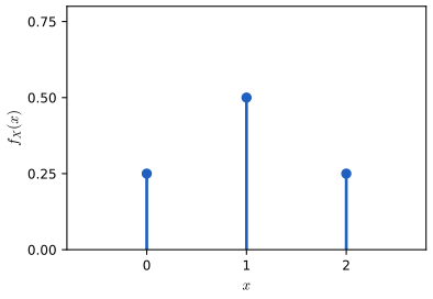
fig_2_2. Reproduces Wasserman (2004), Figure 2.2. Download: PDF · SVGDefinition 2.4 (continuous random variable, density; Definition 2.11 of the book) p. 23, (2.2)
\(X\) is continuous if there is a function \(f_X\ge0\) with \(\int_{-\infty}^\infty f_X(x)\,\d x=1\) and, for every \(a\le b\),
\[ \P(a\lt X\lt b)=\int_a^bf_X(x)\,\d x. \tag{2.2} \]\(f_X\) is the probability density function (pdf). Then \(F_X(x)=\int_{-\infty}^xf_X(t)\,\d t\), and \(f_X(x)=F_X'(x)\) at every point \(x\) where \(f_X\) is continuous.
The Uniform(0, 1) law of Example 2.12 has density \(\one\{0\le x\le1\}\) and cdf \(0\), \(x\), \(1\) on \((-\infty,0)\), \([0,1]\), \((1,\infty)\) (Figure 2.3). Example 2.13's \(f(x)=(1+x)^{-2}\) on \(x\ge0\) is a density since \(\int_0^\infty(1+x)^{-2}\d x=[-(1+x)^{-1}]_0^\infty=1\); Example 2.14's \(1/(1+x)\) is not, because its integral diverges logarithmically. The book's warning bears repeating: a density is not a probability. It can exceed 1 (\(f=5\) on \([0,\tfrac15]\)) and can even be unbounded (\(f(x)=\tfrac23x^{-1/3}\) on \((0,1)\) integrates to \([x^{2/3}]_0^1=1\)).
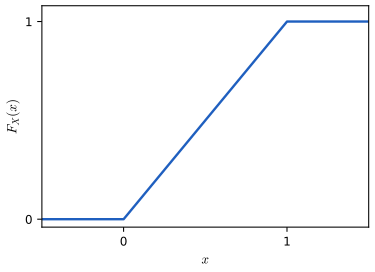
fig_2_3. Reproduces Wasserman (2004), Figure 2.3. Download: PDF · SVGFilling the gap 2.2: in what sense \(f=F'\), and why a density is not unique p. 23; p. 35, footnote 5
(a) If \(f_X\) is a density of \(X\) and \(f_X\) is continuous at \(x\), then \(F_X\) is differentiable at \(x\) with \(F_X'(x)=f_X(x)\). (b) Changing \(f_X\) at finitely (or countably) many points gives another density of the same \(X\); so "\(f_X(x)=F_X'(x)\) at all points where \(F_X\) is differentiable", as the book puts it, holds for a suitable choice of \(f_X\) (or for almost every \(x\)), not for every choice. (c) Not every continuous cdf has a density.
Proof
(a) For \(h\gt0\), \(\frac{F(x+h)-F(x)}h-f(x)\)
(b) An integral does not see the values of the integrand on a set of length zero, so (2.2) is unchanged. Take \(\Unif(0,1)\) with the density changed to \(7\) at \(x=\tfrac12\): it is still a density of the same law, \(F\) is differentiable at \(\tfrac12\) with derivative \(1\ne7\). The correct general statement (Lebesgue's differentiation theorem) is that \(F'(x)\) exists and equals \(f(x)\) for almost every \(x\).
(c) The Cantor function \(F\) is continuous, non-decreasing, 0 at 0 and 1 at 1, and constant on each of the removed middle-third intervals, whose lengths add up to 1. So \(F'=0\) except on the Cantor set, of length 0; if \(F\) had a density \(f\), then \(f=F'=0\) almost everywhere and \(\int f=0\ne1\). By Result 2.2, \(F\) is still the cdf of some \(X\): this \(X\) has \(\P(X=x)=0\) for every \(x\) yet no density. The book's "continuous" in Definition 2.11 therefore means more than "continuous cdf": it means absolutely continuous.
In general every cdf splits uniquely as \(F=aF_d+bF_{ac}+cF_s\), with \(a+b+c=1\): a discrete part (jumps), an absolutely continuous part (with a density) and a singular continuous part like the Cantor function (Lebesgue's decomposition). The distributions met in statistics have \(c=0\); Exercise 2.8 gives one with \(a,b\gt0\). ∎
Result 2.3 (probabilities from the cdf; Lemma 2.15, Exercises 2.1 and 2.3) pp. 24–25
Let \(F\) be the cdf of \(X\). Then
- \(\P(X\lt x)=F(x-)\) and \(\P(X=x)=F(x)-F(x-)\)
\({}=F(x+)-F(x-)\); - \(\P(x\lt X\le y)=F(y)-F(x)\) for \(x\lt y\);
- \(\P(X\gt x)=1-F(x)\);
- if \(X\) is continuous, \(F(b)-F(a)=\P(a\lt X\lt b)\)
\({}=\P(a\le X\lt b)=\P(a\lt X\le b)\) \({}=\P(a\le X\le b)\).
Moreover \(F\) has at most countably many jumps.
Proof
1. \(\{X\le x-1/n\}\uparrow\{X\lt x\}\), so by continuity from below \(F(x-1/n)\to\P(X\lt x)\); since \(F\) is monotone the left limit \(F(x-)\) exists and equals this limit. Then \(\P(X=x)=\P(X\le x)-\P(X\lt x)\)
2. \(\{X\le y\}\) is the disjoint union of \(\{X\le x\}\) and \(\{x\lt X\le y\}\); subtract.
3. Complement of \(\{X\le x\}\).
4. For continuous \(X\), \(\P(X=c)=\lim_{n}\int_{c-1/n}^{c+1/n}f=0\) for every \(c\) (the integrals decrease to \(\P(X=c)\) and tend to 0 because \(f\) is integrable). Adding or removing the end points changes the probability by \(\P(X=a)+\P(X=b)=0\), and 2 gives the value \(F(b)-F(a)\).
Countably many jumps: for each \(k\ge1\), at most \(k\) points can have a jump larger than \(1/k\), because the jumps of \(F\) at distinct points are probabilities of disjoint events and add up to at most 1. The set of all jumps is the union over \(k\) of these finite sets. ∎
Exercise 2.2 is a quick test of item 1: for a jump at \(x=2\), the closed interval \([2,4.8]\) picks up the jump and the half-open \((2,4.8]\) does not (solution, Figure 2.S1).
Definition 2.5 (quantile function; Definition 2.16 of the book) p. 25
The quantile function (inverse cdf) of \(X\) with cdf \(F\) is
\[ F^{-1}(q)=\inf\{x:F(x)\gt q\},\qquad 0\lt q\lt1. \]\(F^{-1}(\tfrac14)\), \(F^{-1}(\tfrac12)\) and \(F^{-1}(\tfrac34)\) are the first quartile, the median and the third quartile. If \(F\) is strictly increasing and continuous, \(F^{-1}(q)\) is the unique \(x\) with \(F(x)=q\).
Two remarks on the definition. At the end points the formula gives \(F^{-1}(1)=\inf\emptyset=+\infty\), and \(F^{-1}(0)=-\infty\) for any law that is unbounded below, so the quantile function is a real-valued function on \((0,1)\); the book's "\(q\in[0,1]\)" needs that reading. And the book uses the strict inequality \(F(x)\gt q\). Most software and many texts use \(\inf\{x:F(x)\ge q\}\) instead. The two agree except at the levels \(q\) where \(F\) is flat, which for continuous strictly increasing \(F\) never happens. For two fair tosses, \(F=\tfrac14\) on \([0,1)\), so the book's first quartile is \(F^{-1}(\tfrac14)=1\) while the other convention gives 0; for a Bernoulli\((\tfrac12)\) the book's median is 1, the other one 0. For sampling the choice is immaterial (a uniform hits a given level with probability zero).
Result 2.4 (the quantile function; inverse-cdf sampling; the probability integral transform; Exercise 2.15) p. 25; p. 45, Exercise 2.15
Let \(F\) satisfy (i)–(iii) of Result 2.2 and let \(F^{-1}\) be its quantile function.
- Switching relation. For \(0\lt u\lt1\) and real \(x\): \(u\lt F(x)\Rightarrow F^{-1}(u)\le x\Rightarrow u\le F(x)\).
- Inverse-cdf sampling. If \(U\sim\Unif(0,1)\), then \(X=F^{-1}(U)\) has cdf \(F\).
- Probability integral transform. If \(X\) has a continuous cdf \(F\), then \(F(X)\sim\Unif(0,1)\). (If \(F\) has a jump, \(F(X)\) is not uniform.)
Proof
(a) If \(u\lt F(x)\) then \(x\) belongs to \(\{t:F(t)\gt u\}\), so the infimum \(F^{-1}(u)\) is at most \(x\). Conversely suppose \(F^{-1}(u)\le x\). For every \(n\) there is \(t_n\lt F^{-1}(u)+1/n\le x+1/n\) with \(F(t_n)\gt u\) (definition of the infimum), and by monotonicity \(F(x+1/n)\ge F(t_n)\gt u\). Letting \(n\to\infty\) and using right-continuity, \(F(x)\ge u\).
(b) By (a), \(\{U\lt F(x)\}\subset\{F^{-1}(U)\le x\}\)
(c) Let \(F\) be continuous and \(0\lt u\lt1\). Put \(x_u=F^{-1}(u)\). By continuity and the intermediate value theorem the set \(\{x:F(x)=u\}\) is a non-empty closed interval, and \(x_u\) is its right end point (the book's convention), so \(F(x_u)=u\) and \(F(x)\gt u\) for \(x\gt x_u\). Hence \(\{F(X)\le u\}=\{X\le x_u\}\), up to the event \(\{F(X)=u, X\gt x_u\}\), which is empty. So \(\P(F(X)\le u)=F(x_u)=u\). If \(F\) jumps at \(x_0\) from \(a=F(x_0-)\) to \(b=F(x_0)\), then \(F(X)\) never takes values in \((a,b)\), so it cannot be uniform. ∎
Part (b) is the "universal random number generator" of Exercise 2.15, and it is what proves the converse in Result 2.2. For the exponential law, \(F(x)=1-e^{-x/\beta}\) and \(F^{-1}(u)=-\beta\log(1-u)\) (Exercise 2.9); for a discrete law, \(F^{-1}(u)\) is the first support point whose cumulative probability exceeds \(u\), so the value \(x_k\) is returned exactly when \(u\) falls in an interval of length \(f(x_k)\). Figure 2.S4 shows the exponential generator at work, and the probability integral transform for a gamma variable.
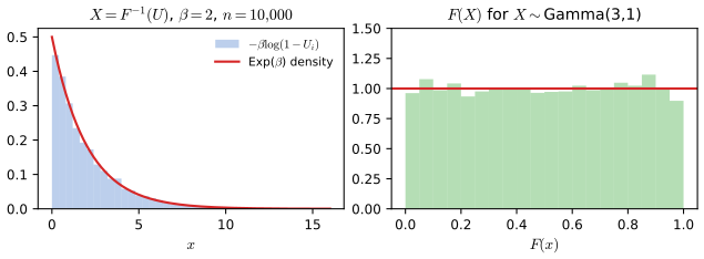
fig_2_s4. Illustrates Wasserman (2004), Exercise 2.15 (supplementary figure). Download: PDF · SVGEquality in distribution. \(X\deq Y\) means \(F_X=F_Y\); by Result 2.1 all probability statements about \(X\) alone and \(Y\) alone then agree. It says nothing about how \(X\) and \(Y\) are related: with \(\P(X=1)=\P(X=-1)=\tfrac12\) and \(Y=-X\), \(X\deq Y\) but \(\P(X=Y)=\P(X=0)=0\).
2.3 Some Important Discrete Random Variables
pp. 25–27 \(X\sim F\) is read "\(X\) has distribution \(F\)". The families below are named by their mass functions; in each, the parameters (\(a\), \(k\), \(p\), \(n\), \(\lambda\)) are fixed numbers, not random variables.
See also (companion courses): Section 3.1 of Foundations of Deep Learning; Section 2.1 of Bayesian and Probabilistic Machine Learning; Section 1.3 of Statistical Methods for Modern Biology. Their means and variances are in Section 3.4 of this course.
| Law | Mass function | Values |
|---|---|---|
| Point mass \(\delta_a\) | \(f(a)=1\) | \(a\) |
| Discrete uniform | \(f(x)=1/k\) | \(1,\dots,k\) |
| \(\Bern(p)\) | \(f(x)=p^x(1-p)^{1-x}\) | \(0,1\) |
| \(\Bin(n,p)\) | \(f(x)=\binom nx p^x(1-p)^{n-x}\) | \(0,\dots,n\) |
| \(\Geom(p)\) | \(f(k)=p(1-p)^{k-1}\) | \(1,2,\dots\) |
| \(\Poi(\lambda)\) | \(f(x)=e^{-\lambda}\lambda^x/x!\) | \(0,1,2,\dots\) |
Result 2.5 (the binomial distribution) p. 26
(a) If \(n\) tosses are independent, each a head with probability \(p\), the number of heads \(X\) has \(\P(X=x)=\binom nxp^x(1-p)^{n-x}\), \(x=0,\dots,n\), and these probabilities add up to 1. (b) If \(X_1\sim\Bin(n_1,p)\) and \(X_2\sim\Bin(n_2,p)\) are independent, then \(X_1+X_2\sim\Bin(n_1+n_2,p)\).
Proof
(a) An outcome is a sequence in \(\{H,T\}^n\). By independence a particular sequence with \(x\) heads has probability \(p^x(1-p)^{n-x}\), whatever the positions of the heads. The event \(\{X=x\}\) is the disjoint union of the \(\binom nx\) sequences with exactly \(x\) heads (choose the positions of the heads), so its probability is \(\binom nxp^x(1-p)^{n-x}\). The binomial theorem gives \(\sum_{x=0}^n\binom nxp^x(1-p)^{n-x}\)
(b) For \(0\le z\le n_1+n_2\), by independence and Vandermonde's identity \(\sum_x\binom{n_1}x\binom{n_2}{z-x}=\binom{n_1+n_2}z\) (count the \(z\)-subsets of a set of size \(n_1+n_2\) by how many fall in the first \(n_1\)),
\[ \P(X_1+X_2=z)=\sum_x\binom{n_1}xp^x(1-p)^{n_1-x}\binom{n_2}{z-x}p^{z-x}(1-p)^{n_2-z+x}=\binom{n_1+n_2}zp^z(1-p)^{n_1+n_2-z}. \]Without independence the statement fails: \(X_2=X_1\sim\Bin(1,\tfrac12)\) gives \(X_1+X_2\in\{0,2\}\). ∎
Result 2.6 (geometric and Poisson laws) pp. 26–27
(a) \(\sum_{k\ge1}p(1-p)^{k-1}=1\) for \(0\lt p\le1\), and \(X\sim\Geom(p)\) is the number of independent tosses up to and including the first head. (b) \(\sum_{x\ge0}e^{-\lambda}\lambda^x/x!=1\). (c) If \(X_1\sim\Poi(\lambda_1)\) and \(X_2\sim\Poi(\lambda_2)\) are independent, then \(X_1+X_2\sim\Poi(\lambda_1+\lambda_2)\). (d) If \(X_n\sim\Bin(n,p_n)\) with \(np_n\to\lambda\), then \(\P(X_n=x)\to e^{-\lambda}\lambda^x/x!\) for every \(x\).
Proof
(a) Geometric series: \(p\sum_{k\ge1}(1-p)^{k-1}\)
(b) The exponential series \(\sum_x\lambda^x/x!=e^\lambda\).
(c) By independence and the binomial theorem,
\[ \P(X_1+X_2=z)=\sum_{x=0}^ze^{-\lambda_1}\frac{\lambda_1^x}{x!}e^{-\lambda_2}\frac{\lambda_2^{z-x}}{(z-x)!}=\frac{e^{-(\lambda_1+\lambda_2)}}{z!}\sum_{x=0}^z\binom zx\lambda_1^x\lambda_2^{z-x}=e^{-(\lambda_1+\lambda_2)}\frac{(\lambda_1+\lambda_2)^z}{z!}. \](d) Write \(\lambda_n=np_n\). Then \[\P(X_n=x)=\frac{n(n-1)\cdots(n-x+1)}{n^x}\cdot\frac{\lambda_n^x}{x!}\cdot\big(1-\frac{\lambda_n}n\big)^n\big(1-\frac{\lambda_n}n\big)^{-x}\]. The first factor tends to 1 (\(x\) is fixed), the second to \(\lambda^x/x!\), the last to 1, and \((1-\lambda_n/n)^n=\exp\{n\log(1-\lambda_n/n)\}\)
Part (d) is why the Poisson law models counts of rare events (decays, accidents): many independent chances, each small. A quantitative version (Le Cam's inequality) is in Result 1.4 of Statistical Methods for Modern Biology. The inverse-cdf demonstration samples the Poisson law by searching its cdf.
The sample space is still there. The book's warning on page 27 builds a Bernoulli variable on \(\Omega=[0,1]\) with length as probability: \(X(\omega)=\one\{\omega\le p\}\). The proof of Result 2.2 does the same for every distribution, with \(X(\omega)=F^{-1}(\omega)\).
2.4 Some Important Continuous Random Variables
pp. 27–30
See also (companion courses): Result 2.2 of Foundations of Deep Learning (the Gaussian integral); Result 2.2 (the beta), Result 2.17 (the gamma) and Result 2.19 (Student's t) of Bayesian and Probabilistic Machine Learning; the first-year notes The chi-squared and t distributions.
| Law | Density | Range |
|---|---|---|
| \(\Unif(a,b)\) | \(1/(b-a)\) | \(a\le x\le b\) |
| \(\N(\mu,\sigma^2)\) | \(\frac1{\sigma\sqrt{2\pi}}\exp\{-\frac{(x-\mu)^2}{2\sigma^2}\}\) (2.3) | \(x\in\R\) |
| \(\Exp(\beta)\) | \(\frac1\beta e^{-x/\beta}\) | \(x\gt0\) |
| \(\Gam(\alpha,\beta)\) | \(\frac{1}{\beta^\alpha\Gamma(\alpha)}x^{\alpha-1}e^{-x/\beta}\) | \(x\gt0\) |
| \(\mathrm{Beta}(\alpha,\beta)\) | \(\frac{\Gamma(\alpha+\beta)}{\Gamma(\alpha)\Gamma(\beta)}x^{\alpha-1}(1-x)^{\beta-1}\) | \(0\lt x\lt1\) |
| \(t_\nu\) | \(\frac{\Gamma(\frac{\nu+1}2)}{\sqrt{\nu\pi}\,\Gamma(\frac\nu2)}\big(1+\frac{x^2}\nu\big)^{-(\nu+1)/2}\) | \(x\in\R\) |
| Cauchy | \(\frac1{\pi(1+x^2)}\) | \(x\in\R\) |
| \(\chi^2_p\) | \(\frac1{\Gamma(p/2)2^{p/2}}x^{p/2-1}e^{-x/2}\) | \(x\gt0\) |
The \(t\) density is written with the factor \(1/\sqrt{\nu\pi}\), which the book's first printing omits (listed in the author's errata; see Notes on the book).
Result 2.7 (the Normal family) pp. 28–29
(a) (2.3) integrates to 1. (b) If \(X\sim\N(\mu,\sigma^2)\) then \(Z=(X-\mu)/\sigma\sim\N(0,1)\); if \(Z\sim\N(0,1)\) then \(\mu+\sigma Z\sim\N(\mu,\sigma^2)\). Hence \(\P(a\lt X\lt b)=\Phi(\frac{b-\mu}\sigma)-\Phi(\frac{a-\mu}\sigma)\). (c) Sums of independent Normals are Normal, with the means and the variances added: this is fact (iii) on page 28, proved in Result 2.20.
Proof
(a) Let \(I=\int_\R e^{-z^2/2}\d z\). Then \(I^2=\iint e^{-(x^2+y^2)/2}\d x\,\d y\); in polar coordinates (\(\d x\,\d y=r\,\d r\,\d\theta\), Result 2.18) this is \(\int_0^{2\pi}\int_0^\infty e^{-r^2/2}r\,\d r\,\d\theta=2\pi\), so \(I=\sqrt{2\pi}\). Substituting \(z=(x-\mu)/\sigma\) in (2.3) gives \(\int=I/\sqrt{2\pi}=1\). (Foundations of Deep Learning, Result 2.2, gives the same argument in full.)
(b) \(\P(Z\le z)=\P(X\le\mu+\sigma z)\)
Example 2.17: for \(X\sim\N(3,5)\), \(\P(X\gt1)=1-\Phi(-2/\sqrt5)\)scipy.stats.norm.cdf and .ppf).
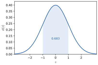
fig_2_4. Reproduces Wasserman (2004), Figure 2.4. Download: PDF · SVGResult 2.8 (the gamma and beta integrals) pp. 29–30
For \(\alpha,\beta\gt0\), with \(\Gamma(\alpha)=\int_0^\infty y^{\alpha-1}e^{-y}\d y\):
- \(\Gamma(\alpha)\) is finite, \(\Gamma(\alpha+1)=\alpha\Gamma(\alpha)\), \(\Gamma(n)=(n-1)!\) and \(\Gamma(\tfrac12)=\sqrt\pi\);
- the \(\Gam(\alpha,\beta)\) density integrates to 1, and \(\Gam(1,\beta)=\Exp(\beta)\);
- \(B(\alpha,\beta)=\int_0^1x^{\alpha-1}(1-x)^{\beta-1}\d x\)
\({}=\Gamma(\alpha)\Gamma(\beta)/\Gamma(\alpha+\beta)\), so the Beta density integrates to 1.
Proof
(a) Near 0 the integrand is at most \(y^{\alpha-1}\), integrable since \(\alpha\gt0\); for large \(y\), \(y^{\alpha-1}e^{-y}\le e^{-y/2}\). Integrating by parts, \(\Gamma(\alpha+1)=[-y^\alpha e^{-y}]_0^\infty+\alpha\int y^{\alpha-1}e^{-y}\d y\)
(b) Substitute \(y=x/\beta\): \(\int_0^\infty x^{\alpha-1}e^{-x/\beta}\d x=\beta^\alpha\Gamma(\alpha)\).
(c) By Fubini (the integrand is non-negative),
\[ \Gamma(\alpha)\Gamma(\beta)=\int_0^\infty\!\!\int_0^\infty u^{\alpha-1}v^{\beta-1}e^{-(u+v)}\,\d u\,\d v. \]Change variables to \(s=u+v\in(0,\infty)\), \(x=u/(u+v)\in(0,1)\); the inverse map \(u=sx\), \(v=s(1-x)\) has Jacobian determinant \(\big|\begin{smallmatrix}x&s\\1-x&-s\end{smallmatrix}\big|=-s\), so \(\d u\,\d v=s\,\d s\,\d x\) (Result 2.18) and
\[ \Gamma(\alpha)\Gamma(\beta)=\int_0^1\!\!\int_0^\infty (sx)^{\alpha-1}(s(1-x))^{\beta-1}e^{-s}s\,\d s\,\d x=\Gamma(\alpha+\beta)\,B(\alpha,\beta). \]∎
The same change of variables says more: if \(U\sim\Gam(\alpha,1)\) and \(V\sim\Gam(\beta,1)\) are independent, then \(U+V\sim\Gam(\alpha+\beta,1)\) and \(U/(U+V)\sim\mathrm{Beta}(\alpha,\beta)\), independent of each other; the joint density of \((s,x)\) above factorises. This gives the book's closure statement for gamma sums (Result 2.20).
Result 2.9 (Student's \(t\) and the Cauchy law) p. 30
(a) The \(t_\nu\) density (with the factor \(1/\sqrt{\nu\pi}\)) integrates to 1; the Cauchy law is \(t_1\). (b) As \(\nu\to\infty\), the \(t_\nu\) density converges to \(\phi\) at every \(x\), and the \(t_\nu\) cdf converges to \(\Phi\) uniformly; this is the sense of "the Normal corresponds to \(\nu=\infty\)".
Proof
(a) By symmetry and the substitution \(w=x^2/\nu\), then \(s=w/(1+w)\) (so \(1+w=1/(1-s)\), \(\d w=\d s/(1-s)^2\)):
\[ \int_\R\Big(1+\frac{x^2}\nu\Big)^{-\frac{\nu+1}2}\d x=\sqrt\nu\int_0^\infty w^{-1/2}(1+w)^{-\frac{\nu+1}2}\d w=\sqrt\nu\int_0^1s^{-1/2}(1-s)^{\frac\nu2-1}\d s=\sqrt\nu\,B\big(\tfrac12,\tfrac\nu2\big). \]By Result 2.8(c) and \(\Gamma(\frac12)=\sqrt\pi\) this is \(\sqrt{\nu\pi}\,\Gamma(\frac\nu2)/\Gamma(\frac{\nu+1}2)\), the reciprocal of the constant. For \(\nu=1\), \(\Gamma(1)/(\sqrt\pi\Gamma(\frac12))=1/\pi\): the Cauchy density, whose integral the book computes with \(\tan^{-1}\).
(b) \(\log(1+x^2/\nu)^{-(\nu+1)/2}\to-x^2/2\) for each \(x\), and by Stirling's formula \(\Gamma(\frac{\nu+1}2)/(\sqrt{\nu}\,\Gamma(\frac\nu2))\to1/\sqrt2\), so the constant tends to \(1/\sqrt{2\pi}\). Pointwise convergence of densities to a density implies \(\int|f_\nu-\phi|\to0\) (Scheffé's lemma: \(\int(\phi-f_\nu)^+\to0\) by dominated convergence, since \(0\le(\phi-f_\nu)^+\le\phi\), and \(\int|f_\nu-\phi|=2\int(\phi-f_\nu)^+\) because both integrate to 1), and \(\sup_x|F_\nu(x)-\Phi(x)|\le\int|f_\nu-\phi|\). Numerically, \(\sup_x|t_\nu(x)-\phi(x)|\approx0.136/\nu\). ∎
Result 2.10 (the \(\chi^2\) family) p. 30
\(\chi^2_p=\Gam(p/2,2)\). If \(Z\sim\N(0,1)\) then \(Z^2\sim\chi^2_1\), and if \(Z_1,\dots,Z_p\) are independent \(\N(0,1)\), then \(\sum_iZ_i^2\sim\chi^2_p\).
Proof
The first claim is a comparison of densities. For \(y\gt0\), \(\P(Z^2\le y)=\P(-\sqrt y\le Z\le\sqrt y)\)
using \(\Gamma(\tfrac12)=\sqrt\pi\): the \(\chi^2_1\) density. The \(Z_i^2\) are independent (Result 2.13) and \(\Gam(\frac12,2)\), and gamma laws with a common scale add their shapes (Result 2.20), so the sum is \(\Gam(\frac p2,2)=\chi^2_p\). ∎
The transformation demonstration shows the two branches of \(Z^2\) adding up (choose N(0, 1) and \(x^2\)).
2.5 Bivariate Distributions
pp. 31–32 For a pair of discrete random variables the joint mass function is \(f(x,y)=\P(X=x,Y=y)\). In Example 2.18, \(X,Y\in\{0,1\}\) with \(f(0,0)=\tfrac19\), \(f(0,1)=f(1,0)=\tfrac29\), \(f(1,1)=\tfrac49\); notice that every entry is the product of its row and column totals \((\tfrac13,\tfrac23)\), so (by Section 2.7) these two variables happen to be independent.
Definition 2.6 (joint density and joint cdf; Definition 2.19 of the book) p. 31
A function \(f(x,y)\) is a joint density for \((X,Y)\) if (i) \(f\ge0\), (ii) \(\iint f(x,y)\,\d x\,\d y=1\) and (iii) \(\P((X,Y)\in A)=\iint_Af(x,y)\,\d x\,\d y\) for every (Borel) \(A\subset\R^2\). In both cases the joint cdf is \(F_{X,Y}(x,y)=\P(X\le x,Y\le y)\).
Examples 2.20 and 2.21: on the unit square the uniform density gives \(\P(X\lt\tfrac12,Y\lt\tfrac12)=\tfrac14\), the area of the quarter square; and \(f(x,y)=x+y\) integrates to \(\tfrac12+\tfrac12=1\).
Example 2.22 (non-rectangular support). Let \(f(x,y)=c\,x^2y\) on \(\{x^2\le y\le1\}\), so \(-1\le x\le1\). Integrating \(y\) first, \(\int_{x^2}^1y\,\d y=(1-x^4)/2\), and
\[ 1=c\int_{-1}^1x^2\frac{1-x^4}2\,\d x=c\Big(\frac13-\frac17\Big)=\frac{4c}{21},\qquad c=\frac{21}4. \]The event \(\{X\ge Y\}\) meets the support in \(\{0\le x\le1,\ x^2\le y\le x\}\) (the hatched region of Figure 2.5; for \(x\lt0\), \(y\ge x^2\ge0\gt x\)), so \(\P(X\ge Y)=\frac{21}4\int_0^1x^2\frac{x^2-x^4}2\d x\)
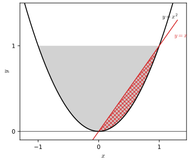
fig_2_5. Reproduces Wasserman (2004), Figure 2.5. Download: PDF · SVG2.6 Marginal Distributions
pp. 33–34
See also (companion course): the sum rule for densities, Filling the gap 2.2 of Foundations of Deep Learning.
Definition 2.7 (marginal mass functions and densities; Definitions 2.23 and 2.25 of the book) pp. 33–34, (2.4)–(2.6)
\[ f_X(x)=\P(X=x)=\sum_y\P(X=x,Y=y)=\sum_yf(x,y), \tag{2.4} \] \[ f_Y(y)=\P(Y=y)=\sum_x\P(X=x,Y=y)=\sum_xf(x,y), \tag{2.5} \]and for continuous random variables
\[ f_X(x)=\int f(x,y)\,\d y,\qquad f_Y(y)=\int f(x,y)\,\d x. \tag{2.6} \]Why (2.6) is right: for a Borel \(A\subset\R\), \(\P(X\in A)=\P((X,Y)\in A\times\R)\)
2.7 Independent Random Variables
pp. 34–36
See also (companion course): Section 2.1.6 of Foundations of Deep Learning.
Definition 2.8 (independent random variables; Definition 2.29 of the book) p. 34, (2.7)
\(X\) and \(Y\) are independent, \(X\ind Y\), if for every (Borel) \(A\) and \(B\)
\[ \P(X\in A,Y\in B)=\P(X\in A)\,\P(Y\in B). \tag{2.7} \]Result 2.11 (independence means a factorised density; Theorem 2.30 and Exercise 2.5) p. 35, footnote 5; p. 44
(a) Discrete case: \(X\ind Y\) if and only if \(f_{X,Y}(x,y)=f_X(x)f_Y(y)\) for all \(x,y\). (b) Continuous case: if \((X,Y)\) has joint density \(f_{X,Y}\), then \(X\ind Y\) if and only if \(f_{X,Y}(x,y)=f_X(x)f_Y(y)\) for almost every \((x,y)\), that is, if and only if the product of the marginals is a joint density.
Proof
(a) If \(X\ind Y\), take \(A=\{x\}\), \(B=\{y\}\) in (2.7). Conversely, if the mass function factorises, then for any \(A,B\), \[\P(X\in A,Y\in B)=\sum_{x\in A}\sum_{y\in B}f_X(x)f_Y(y)=\Big(\sum_{x\in A}f_X(x)\Big)\Big(\sum_{y\in B}f_Y(y)\Big)\] (a rearrangement of a series of non-negative terms).
(b) "If": by Fubini, \(\P(X\in A,Y\in B)\)
"Almost every" is the precise form of the book's footnote 5: a density can be changed on a set of area zero (a line, say) without changing any probability, so a pointwise identity "for all \(x,y\)" cannot be required.
Example 2.31 contrasts a table whose four cells are all \(\tfrac14\) (independent, every cell is \(\tfrac12\cdot\tfrac12\)) with the diagonal table \(f(0,0)=f(1,1)=\tfrac12\) (dependent: \(f(0,1)=0\ne\tfrac14\)). In Example 2.32, \(X,Y\) are independent with density \(2x\) on \([0,1]\), the joint density is \(4xy\) on the square, and
\[ \P(X+Y\le1)=4\int_0^1x\int_0^{1-x}y\,\d y\,\d x=2\int_0^1x(1-x)^2\,\d x=2\cdot\frac1{12}=\frac16. \]Result 2.12 (any factorisation on a rectangle; Theorem 2.33 and Exercise 2.12) p. 36; p. 45
Suppose \((X,Y)\) has a joint density with \(f(x,y)=g(x)h(y)\) for all \((x,y)\in\R^2\), for some non-negative functions \(g,h\) (not necessarily densities). Then \(X\ind Y\), with \(f_X=g/\int g\) and \(f_Y=h/\int h\). The identity must hold on the whole plane, zeros included; this forces the set where \(f\gt0\) to be a product set \(\{g\gt0\}\times\{h\gt0\}\), which is the book's condition that "the range of \(X\) and \(Y\) is a rectangle".
Proof
Let \(G=\int g\) and \(H=\int h\). By Fubini \(1=\iint g(x)h(y)\,\d x\,\d y=GH\), so both are finite and positive. From (2.6), \(f_X(x)=g(x)H\) and \(f_Y(y)=Gh(y)\), hence \(f_X(x)f_Y(y)=GH\,g(x)h(y)=f(x,y)\), and Result 2.11(b) applies. ∎
Why the rectangle matters. In Example 2.28, \(f(x,y)=\frac{21}4x^2y\,\one\{x^2\le y\le1\}\). The formula \(x^2y\) factorises, but the indicator does not, so \(f\) is not of the form \(g(x)h(y)\). And indeed \(X\) and \(Y\) are dependent: \(f_X(0.9)\gt0\) and \(f_Y(0.5)\gt0\), yet \(f=0\) on the whole neighbourhood of \((0.9,0.5)\) where \(y\lt x^2\), so \(f\ne f_Xf_Y\) on a set of positive area. Knowing \(X=0.9\) forces \(Y\ge0.81\).
Example 2.34: \(2e^{-(x+2y)}\) on \((0,\infty)^2\) is \(g(x)h(y)\) with \(g=2e^{-x}\), \(h=e^{-2y}\) on a rectangle, so \(X\ind Y\), \(X\sim\Exp(1)\), \(Y\sim\Exp(\tfrac12)\).
2.8 Conditional Distributions
pp. 36–38
See also (companion course): the product rule and Bayes' theorem for densities, Filling the gap 2.2 of Foundations of Deep Learning.
Definition 2.9 (conditional mass function and density; Definitions 2.35 and 2.36 of the book) pp. 36–37
If \(f_Y(y)\gt0\), the conditional mass function (discrete case) or conditional density (continuous case) of \(X\) given \(Y=y\) is
\[ f_{X\given Y}(x\given y)=\frac{f_{X,Y}(x,y)}{f_Y(y)}, \]and in the continuous case \(\P(X\in A\given Y=y)=\int_Af_{X\given Y}(x\given y)\,\d x\).
In the discrete case this is the elementary \(\P(X=x\given Y=y)\)
Filling the gap 2.3: the conditional density as a limit, and the Borel paradox p. 36, footnote 6
(a) Suppose that \(f_{X,Y}(x,\cdot)\) is continuous at \(y\) for every \(x\), that \(f_{X,Y}(x,t)\le g(x)\) for \(t\) near \(y\) with \(\int g\lt\infty\), and that \(f_Y(y)\gt0\). Then for every Borel \(A\)
\[ \lim_{h\downarrow0}\P\big(X\in A\given y\lt Y\le y+h\big)=\int_Af_{X\given Y}(x\given y)\,\d x. \](b) The answer depends on how the null event is approached. Let \(X,Y\) be independent \(\N(0,1)\). Conditioning on \(\{X-Y=0\}\) through \(D=X-Y\) gives \(f(x\given D=0)\propto\phi(x)^2\propto e^{-x^2}\), a \(\N(0,\tfrac12)\) density; conditioning on the same set through \(R=X/Y\) gives \(f(x\given R=1)\propto|x|e^{-x^2}\).
Proof
(a) Write the conditional probability as a ratio of two averages over \((y,y+h]\):
\[ \P(X\in A\given y\lt Y\le y+h)=\frac{\int_A\frac1h\int_y^{y+h}f(x,t)\,\d t\,\d x}{\int_\R\frac1h\int_y^{y+h}f(x,t)\,\d t\,\d x}. \]For each \(x\), the inner average tends to \(f(x,y)\) by continuity, and it is bounded by \(g(x)\) for small \(h\). By dominated convergence the numerator tends to \(\int_Af(x,y)\,\d x\) and the denominator to \(\int f(x,y)\,\d x=f_Y(y)\gt0\).
(b) For \(D\): the map \((x,y)\mapsto(x,d)=(x,x-y)\) has inverse \(y=x-d\) with Jacobian determinant of absolute value 1 (Result 2.18), so \(f_{X,D}(x,d)=\phi(x)\phi(x-d)\) and at \(d=0\) the conditional density is proportional to \(\phi(x)^2\). For \(R\): the map \((x,y)\mapsto(x,r)=(x,x/y)\) has inverse \(y=x/r\) with \(|\partial y/\partial r|=|x|/r^2\), so \(f_{X,R}(x,r)=\phi(x)\phi(x/r)|x|/r^2\) and at \(r=1\) it is proportional to \(|x|\phi(x)^2\). Both conditionings describe "\(X=Y\)", but the thin strips \(\{|X-Y|\lt\varepsilon\}\) and \(\{|X/Y-1|\lt\varepsilon\}\) are different shapes (the second is a wedge, wider far from the origin), and (a) says the limit follows the strips. ∎
So a conditional density given \(Y=y\) is meaningful as a function of \(y\) for a fixed conditioning variable \(Y\), not as a property of the set \(\{Y=y\}\). The measure-theoretic definition (conditional expectation given a \(\sigma\)-field) makes this precise.
From the definition, \(f_{X,Y}(x,y)=f_{X\given Y}(x\given y)f_Y(y)\)
- Example 2.37. Uniform on the square: \(f_{X\given Y}(x\given y)=1\) on \([0,1]\), so \(X\given Y=y\sim\Unif(0,1)\) for every \(y\).
- Example 2.38. \(f=x+y\): \(f_{X\given Y}(x\given y)=(x+y)/(y+\tfrac12)\), and \[\P\big(X\lt\tfrac14\given Y=\tfrac13\big)=\frac{\tfrac1{32}+\tfrac1{12}}{\tfrac13+\tfrac12}=\frac{11}{96}\cdot\frac65=\frac{11}{80}.\]
- Example 2.39 (a two-stage model). \(X\sim\Unif(0,1)\), then \(Y\given X=x\sim\Unif(x,1)\). The joint density is \(1/(1-x)\) on \(0\lt x\lt y\lt1\), and \(f_Y(y)=\int_0^y\frac{\d x}{1-x}=-\log(1-y)\), a density increasing to \(+\infty\) as \(y\to1\) (it integrates to \(\int_0^1-\log(1-y)\,\d y=1\)). A simulation of \(10^5\) pairs agrees with it.
- Example 2.40. In Example 2.28, \(f_{Y\given X}(y\given x)=2y/(1-x^4)\) on \(x^2\le y\le1\); at \(x=\tfrac12\) this is \(32y/15\) on \([\tfrac14,1]\), and \(\P(Y\ge\tfrac34\given X=\tfrac12)=\frac{16}{15}\big(1-\tfrac9{16}\big)=\tfrac7{15}\).
2.9 Multivariate Distributions and iid Samples
pp. 38–39 A random vector \(X=(X_1,\dots,X_n)\) has a joint mass function or density \(f(x_1,\dots,x_n)\); marginals and conditionals are formed as in two dimensions, by summing or integrating out the coordinates not wanted and dividing by the marginal of the coordinates conditioned on. \(X_1,\dots,X_n\) are independent if for all \(A_1,\dots,A_n\)
\[ \P(X_1\in A_1,\dots,X_n\in A_n)=\prod_{i=1}^n\P(X_i\in A_i), \tag{2.8} \]and, exactly as in Result 2.11, this holds if and only if \(f(x_1,\dots,x_n)=\prod_if_{X_i}(x_i)\) (almost everywhere, in the continuous case).
Definition 2.10 (iid sample; Definition 2.41 of the book) p. 39
If \(X_1,\dots,X_n\) are independent and each has the same marginal cdf \(F\), they are independent and identically distributed (iid), written \(X_1,\dots,X_n\sim F\) (or \(\sim f\) for a density): a random sample of size \(n\) from \(F\). Their joint density is \(\prod_if(x_i)\).
Result 2.13 (functions of independent variables; Exercise 2.10) p. 45
(a) If \(X\ind Y\) then \(g(X)\ind h(Y)\) for any (Borel) functions \(g,h\). (b) More generally, if \(X_1,\dots,X_n\) are independent and \(I_1,\dots,I_m\) are disjoint groups of indices, then functions of the groups, \(g_1(X_{I_1}),\dots,g_m(X_{I_m})\), are independent.
Proof
(a) \(\{g(X)\in A\}=\{X\in g^{-1}(A)\}\) and \(g^{-1}(A)\) is a Borel set, so \(\P(g(X)\in A,h(Y)\in B)\)
(b) It is enough to show that the vectors \(X_{I_1},\dots,X_{I_m}\) are independent, then apply (a) to each. Take two groups for clarity, \(U=(X_1,\dots,X_k)\) and \(V=(X_{k+1},\dots,X_n)\). By (2.8), \(\P(U\in C,V\in D)=\P(U\in C)\P(V\in D)\) when \(C\) and \(D\) are products of Borel sets. Fix such a \(D\); both sides are finite measures in \(C\) that agree on the \(\pi\)-system of products, so (as in Result 2.1) they agree for all Borel \(C\subset\R^k\). Now fix any Borel \(C\) and repeat in \(D\). ∎
Result 2.13 is used constantly: the \(Z_i^2\) of Result 2.10 are independent, the sample mean of the first half of a sample is independent of the sample mean of the second half, and so on. Independence of \(n\) variables needs the full product rule (2.8): three variables can be independent in pairs without being independent. For example, if \(X,Y\) are independent fair bits and \(Z=X\oplus Y\) (their sum modulo 2), any two of \(X,Y,Z\) are independent but \(Z\) is a function of the other two (the same example for events is in Result 1.G of the Chapter 1 notes).
2.10 Two Important Multivariate Distributions
pp. 39–40
See also (companion courses): the multinomial in Result 1.8 of Statistical Methods for Modern Biology and Result 3.3 of Foundations of Deep Learning; the multivariate Gaussian in Section 3.2 of Foundations of Deep Learning (Results 3.7–3.9) and Section 2.3 of Bayesian and Probabilistic Machine Learning (Results 2.9, 2.10). Their means and covariances: Filling the gap 3.7 of this course.
Multinomial. An urn has balls of \(k\) colours, colour \(j\) drawn with probability \(p_j\) (\(p_j\ge0\), \(\sum_jp_j=1\)). Draw \(n\) times independently with replacement and let \(X_j\) be the number of draws of colour \(j\); then \(\sum_jX_j=n\) and \(X=(X_1,\dots,X_k)\sim\Mult(n,p)\) with
\[ f(x)=\binom n{x_1\,\cdots\,x_k}p_1^{x_1}\cdots p_k^{x_k},\qquad\binom n{x_1\,\cdots\,x_k}=\frac{n!}{x_1!\cdots x_k!}. \tag{2.9} \]Result 2.14 (the multinomial mass function and its margins; (2.9) and Lemma 2.42) p. 39
(a) (2.9) is the probability of the counts \(x\) (with \(x_j\ge0\), \(\sum x_j=n\)), and these probabilities add up to 1. (b) Each \(X_j\sim\Bin(n,p_j)\). (c) More generally, merging colours into groups gives a multinomial with the summed probabilities.
Proof
(a) A particular sequence of \(n\) colours with \(x_j\) draws of colour \(j\) has probability \(\prod_jp_j^{x_j}\) by independence. The number of such sequences is the number of ways to assign the \(n\) positions to colours with these counts: choose the \(x_1\) positions of colour 1, then \(x_2\) of the remaining, and so on, \(\binom n{x_1}\binom{n-x_1}{x_2}\cdots=\frac{n!}{x_1!\cdots x_k!}\). The multinomial theorem gives \(\sum_xf(x)=(p_1+\dots+p_k)^n=1\).
(c) and (b). Each draw falls in group \(G\) with probability \(\sum_{j\in G}p_j\), independently of the other draws, so the group counts are the counts of a multinomial experiment with these probabilities, by (a). With the two groups \(\{j\}\) and "not \(j\)" this is a binomial experiment for \(X_j\) with success probability \(p_j\). (An algebraic proof sums (2.9) over the other coordinates with the multinomial theorem.) ∎
Multivariate Normal. If \(Z_1,\dots,Z_k\) are independent \(\N(0,1)\), the vector \(Z\) has density \(\prod_i\phi(z_i)=(2\pi)^{-k/2}\exp(-\tfrac12z^\T z)\), the standard multivariate Normal \(\N(0,I)\). More generally \(X\sim\N(\mu,\Sigma)\) if it has density
\[ f(x;\mu,\Sigma)=\frac{1}{(2\pi)^{k/2}|\Sigma|^{1/2}}\exp\Big\{-\frac12(x-\mu)^\T\Sigma^{-1}(x-\mu)\Big\}, \tag{2.10} \]where \(\mu\in\R^k\) and \(\Sigma\) is a symmetric positive definite \(k\times k\) matrix (\(x^\T\Sigma x\gt0\) for \(x\ne0\)).
Result 2.15 (the square root of \(\Sigma\), and \(\N(\mu,\Sigma)\) as a linear image of \(\N(0,I)\); Theorem 2.43) p. 40
(a) There is a unique symmetric positive definite \(\Sigma^{1/2}\) with \(\Sigma^{1/2}\Sigma^{1/2}=\Sigma\); it is invertible, and \(\Sigma^{-1/2}=(\Sigma^{1/2})^{-1}\) satisfies \(\Sigma^{-1/2}\Sigma\Sigma^{-1/2}=I\). (b) If \(Z\sim\N(0,I)\) then \(X=\mu+\Sigma^{1/2}Z\sim\N(\mu,\Sigma)\); conversely, if \(X\sim\N(\mu,\Sigma)\), then \(\Sigma^{-1/2}(X-\mu)\sim\N(0,I)\). (c) The same holds with \(\Sigma^{1/2}\) replaced by any matrix \(A\) with \(AA^\T=\Sigma\) (for instance the Cholesky factor).
Proof
(a) By the spectral theorem, \(\Sigma=V\Lambda V^\T\) with \(V\) orthogonal and \(\Lambda=\diag(\lambda_1,\dots,\lambda_k)\); each \(\lambda_i=v_i^\T\Sigma v_i\gt0\). Put \(\Sigma^{1/2}=V\Lambda^{1/2}V^\T\): symmetric, positive definite, and \(\Sigma^{1/2}\Sigma^{1/2}=V\Lambda^{1/2}V^\T V\Lambda^{1/2}V^\T\)
(b), (c) Let \(A\) be any invertible matrix with \(AA^\T=\Sigma\), and \(X=\mu+AZ\). The map \(z\mapsto\mu+Az\) is a bijection of \(\R^k\) with inverse \(z=A^{-1}(x-\mu)\), whose Jacobian determinant is \(\det A^{-1}\), of absolute value \(|\det\Sigma|^{-1/2}\) because \((\det A)^2=\det(AA^\T)=|\Sigma|\). By the change-of-variables formula (Result 2.18),
\[ f_X(x)=\frac{1}{(2\pi)^{k/2}}\exp\Big\{-\frac12\big(A^{-1}(x-\mu)\big)^\T A^{-1}(x-\mu)\Big\}\frac1{|\Sigma|^{1/2}}, \]and \((A^{-1})^\T A^{-1}=(AA^\T)^{-1}=\Sigma^{-1}\) turns this into (2.10). The converse is the same computation for the map \(x\mapsto\Sigma^{-1/2}(x-\mu)\). ∎
The parameters are the mean vector and the covariance matrix, \(\E X=\mu\) and \(\Cov(X)=\Sigma\) (Chapter 3; see Filling the gap 3.7). Part (b) is how one simulates a multivariate Normal (Figure 2.S6), and part (c) shows that the choice of square root does not matter.
Partition \(X=(X_a,X_b)\), \(\mu=(\mu_a,\mu_b)\) and \(\Sigma=\begin{pmatrix}\Sigma_{aa}&\Sigma_{ab}\\\Sigma_{ba}&\Sigma_{bb}\end{pmatrix}\).
Result 2.16 (margins, conditionals, linear combinations and the quadratic form; Theorem 2.44) p. 40
Let \(X\sim\N(\mu,\Sigma)\) in \(\R^k\). Then
- \(X_a\sim\N(\mu_a,\Sigma_{aa})\);
- given \(X_a=x_a\), \(X_b\) is Normal with mean \(\mu_b+\Sigma_{ba}\Sigma_{aa}^{-1}(x_a-\mu_a)\) and covariance \(\Sigma_{bb}-\Sigma_{ba}\Sigma_{aa}^{-1}\Sigma_{ab}\);
- for a non-zero vector \(a\), \(a^\T X\sim\N(a^\T\mu,a^\T\Sigma a)\);
- \(V=(X-\mu)^\T\Sigma^{-1}(X-\mu)\sim\chi^2_k\).
Proof
The key identity. Let \(K=\Sigma_{ba}\Sigma_{aa}^{-1}\), \(S=\Sigma_{bb}-K\Sigma_{ab}\) (the Schur complement of \(\Sigma_{aa}\)) and \(L=\begin{pmatrix}I&0\\K&I\end{pmatrix}\). Multiplying out, using \(\Sigma_{ab}=\Sigma_{ba}^\T\),
\[ \Sigma=L\begin{pmatrix}\Sigma_{aa}&0\\0&S\end{pmatrix}L^\T,\qquad L^{-1}=\begin{pmatrix}I&0\\-K&I\end{pmatrix}. \]\(\Sigma_{aa}\) is positive definite (it is \(\Sigma\) restricted to vectors supported on the block \(a\)), and so is the block-diagonal middle matrix \(L^{-1}\Sigma L^{-\T}\), hence \(S\). Taking determinants, \(|\Sigma|=|\Sigma_{aa}|\,|S|\). Inverting, \(\Sigma^{-1}=L^{-\T}\diag(\Sigma_{aa}^{-1},S^{-1})L^{-1}\), and with \(u=x-\mu\), \(L^{-1}u=(u_a,u_b-Ku_a)\), so
\[ (x-\mu)^\T\Sigma^{-1}(x-\mu)=(x_a-\mu_a)^\T\Sigma_{aa}^{-1}(x_a-\mu_a)+\big(x_b-m(x_a)\big)^\T S^{-1}\big(x_b-m(x_a)\big), \]with \(m(x_a)=\mu_b+K(x_a-\mu_a)\). Splitting the constant \((2\pi)^{k/2}|\Sigma|^{1/2}\) the same way, (2.10) factorises:
\[ f(x;\mu,\Sigma)=f\big(x_a;\mu_a,\Sigma_{aa}\big)\cdot f\big(x_b;m(x_a),S\big). \]1 and 2. For fixed \(x_a\), the second factor is a Normal density in \(x_b\) and integrates to 1, so integrating out \(x_b\) leaves \(f_{X_a}(x_a)=f(x_a;\mu_a,\Sigma_{aa})\). Dividing the joint density by it leaves the conditional density \(f(x_b;m(x_a),S)\), which is statement 2.
3. Write \(X=\mu+\Sigma^{1/2}Z\) (Result 2.15). Then \(a^\T X=a^\T\mu+c^\T Z\) with \(c=\Sigma^{1/2}a\ne0\), and \(c^\T Z=\sum_ic_iZ_i\) is a sum of independent \(\N(0,c_i^2)\) variables, hence \(\N(0,\sum c_i^2)\) by Result 2.20; and \(\sum c_i^2=a^\T\Sigma^{1/2}\Sigma^{1/2}a=a^\T\Sigma a\). (Terms with \(c_i=0\) are the constant 0 and can be dropped.)
4. \(V=\|\Sigma^{-1/2}(X-\mu)\|^2=\sum_iZ_i^2\) with \(Z=\Sigma^{-1/2}(X-\mu)\sim\N(0,I)\), which is \(\chi^2_k\) by Result 2.10. ∎
The factorisation also shows that \(X_b-KX_a\) is independent of \(X_a\): the conditional law of \(X_b-KX_a\) given \(X_a=x_a\) is \(\N(\mu_b-K\mu_a,S)\) whatever \(x_a\) is. Foundations of Deep Learning proves 1 and 2 by completing the square in the exponent (Result 3.7, Result 3.9), with the partitioned inverse in Result 3.8.
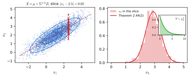
fig_2_s6. Illustrates Wasserman (2004), Theorems 2.43–2.44 (supplementary figure). Download: PDF · SVG2.11 Transformations of Random Variables
pp. 41–42 Given \(X\) and a function \(r\), what is the law of \(Y=r(X)\)? In the discrete case it is immediate: \(f_Y(y)=\P(r(X)=y)=\P(X\in r^{-1}(y))\), the total mass of the preimages of \(y\). In Example 2.45, \(X\in\{-1,0,1\}\) with probabilities \(\tfrac14,\tfrac12,\tfrac14\) and \(Y=X^2\) has \(f_Y(0)=\tfrac12\), \(f_Y(1)=f_X(-1)+f_X(1)=\tfrac12\). For continuous \(X\) the book gives a three-step recipe:
The three steps for a transformation p. 41, (2.11)
- For each \(y\), find the set \(A_y=\{x:r(x)\le y\}\).
- Find the cdf
- The density is \(f_Y(y)=F_Y'(y)\).
See also (companion course): Result 2.6 and Filling the gap 2.7 of Foundations of Deep Learning (one-to-one maps, the moving mode, non-monotone maps).
Example 2.46. \(X\sim\Exp(1)\), \(Y=\log X\): \(A_y=(0,e^y]\), \(F_Y(y)=1-e^{-e^y}\) and \(f_Y(y)=e^ye^{-e^y}\) on \(\R\). Example 2.47. \(X\sim\Unif(-1,3)\), \(Y=X^2\in[0,9)\): for \(0\lt y\lt1\), \(A_y=[-\sqrt y,\sqrt y]\) lies inside \((-1,3)\) and \(F_Y(y)=\tfrac12\sqrt y\); for \(1\le y\lt9\), \(A_y\cap(-1,3)=(-1,\sqrt y]\) and \(F_Y(y)=\tfrac14(\sqrt y+1)\). So \(f_Y(y)=1/(4\sqrt y)\) on \((0,1)\) and \(1/(8\sqrt y)\) on \((1,9)\). Figure 2.S2 compares both with simulations; the density halves at \(y=1\) because the left branch \(x=-\sqrt y\) leaves the support there. The next result explains this without computing \(F_Y\).
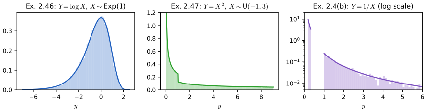
fig_2_s2. Illustrates Wasserman (2004), Section 2.11 (supplementary figure). Download: PDF · SVGResult 2.17 (the transformation formula (2.12) and its many-to-one form; Exercise 2.19) p. 42, (2.12); p. 46
(a) Let \(X\) have density \(f_X\) with \(\P(X\in I)=1\) for an open interval \(I\), and let \(r\) be strictly monotone on \(I\), with an inverse \(s=r^{-1}\) that is continuously differentiable on the interval \(r(I)\). Then \(Y=r(X)\) has density
\[ f_Y(y)=f_X(s(y))\left|\frac{\d s(y)}{\d y}\right|,\qquad y\in r(I), \tag{2.12} \]and \(f_Y=0\) outside \(r(I)\). (b) If instead \(I\) splits into finitely many open intervals \(I_1,\dots,I_m\) (up to finitely many points) on each of which \(r\) is as in (a), with inverses \(s_j\), then
\[ f_Y(y)=\sum_{j:\,y\in r(I_j)}f_X(s_j(y))\,|s_j'(y)|=\sum_{x:\,r(x)=y}\frac{f_X(x)}{|r'(x)|}. \]Proof
(a) Suppose \(r\) is increasing, so \(s\) is increasing and \(s'\ge0\). For \(y\in r(I)\), \(\{Y\le y\}=\{X\le s(y)\}\) (up to the null event \(X\notin I\)), so \(F_Y(y)=F_X(s(y))=\int_{\inf I}^{s(y)}f_X(x)\,\d x\). The substitution \(x=s(t)\), valid for any integrable \(f_X\) because \(s\) is continuously differentiable and increasing, turns this into \(\int_{\inf r(I)}^yf_X(s(t))s'(t)\,\d t\). So \(f_X(s(t))s'(t)\) is a density of \(Y\): no continuity of \(f_X\) is needed, and no differentiation of \(F_Y\). If \(r\) is decreasing, \(\{Y\le y\}=\{X\ge s(y)\}\) and \(F_Y(y)=\int_{s(y)}^{\sup I}f_X\)
(b) For a Borel set \(B\), \(\P(Y\in B)=\sum_j\P(X\in I_j,\ r(X)\in B)\). On \(I_j\), the computation in (a) (with \(f_X\one_{I_j}\) in place of \(f_X\)) gives \(\P(X\in I_j,r(X)\in B)\)
Read the second formula as a balance of probability: the mass \(f_X(x)\,|\d x|\) near each preimage \(x\) of \(y\) is spread over \(|\d y|=|r'(x)|\,|\d x|\). Where \(r\) is steep the mass is thinned out, where it is flat the mass piles up. In Example 2.47, \(y\in(0,1)\) has the two preimages \(\pm\sqrt y\), each contributing \(\tfrac14\cdot\frac1{2\sqrt y}\); \(y\in(1,9)\) has only \(+\sqrt y\) in the support. In Result 2.10, \(Z^2\) has the two symmetric branches \(\pm\sqrt y\). Exercise 2.13 is the log-normal, \(f_Y(y)=\phi(\log y)/y\) (Figure 2.S3); the probability integral transform of Result 2.4(c) is the case \(r=F_X\), where each branch contributes \(f_X(x)\cdot1/f_X(x)=1\).
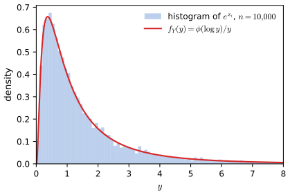
fig_2_s3. Solves Wasserman (2004), Exercise 2.13 (supplementary figure). Download: PDF · SVG2.12 Transformations of Several Random Variables
pp. 42–43 For \(Z=r(X,Y)\) the same three steps apply with \(A_z=\{(x,y):r(x,y)\le z\}\) and \(F_Z(z)=\iint_{A_z}f_{X,Y}(x,y)\,\d x\,\d y\). The hard step is finding \(A_z\).
Example 2.48. \(X_1,X_2\iid\Unif(0,1)\) and \(Y=X_1+X_2\). For \(0\le y\lt1\), \(A_y\) is the triangle with vertices \((0,0),(y,0),(0,y)\), of area \(y^2/2\); for \(1\le y\lt2\) it is the square minus the triangle with vertices \((1,y-1),(1,1),(y-1,1)\), of area \(1-(2-y)^2/2\) (Figure 2.6). So
\[ F_Y(y)=\begin{cases}0&y\lt0\\ y^2/2&0\le y\lt1\\ 1-(2-y)^2/2&1\le y\lt2\\ 1&y\ge2,\end{cases}\qquad f_Y(y)=\begin{cases}y&0\le y\le1\\2-y&1\le y\le2\\0&\text{otherwise.}\end{cases} \]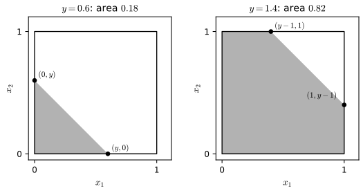
fig_2_6. Reproduces Wasserman (2004), Figure 2.6. Download: PDF · SVGResult 2.18 (the Jacobian formula in several variables) Section 2.12 (not stated in the book)
Let \(X\) be a random vector in \(\R^k\) with density \(f_X\) and \(\P(X\in U)=1\) for an open set \(U\). Let \(r:U\to V\) be a bijection onto an open set \(V\) whose inverse \(s=r^{-1}\) is continuously differentiable, with Jacobian determinant \(J_s(y)=\det\big(\partial s_i(y)/\partial y_j\big)\). Then \(Y=r(X)\) has density
\[ f_Y(y)=f_X(s(y))\,|J_s(y)|,\qquad y\in V, \]and 0 outside \(V\). If \(r\) is only piecewise one-to-one, the contributions of the pieces add, as in Result 2.17(b).
Proof
For a Borel \(B\subset V\), \(\P(Y\in B)=\P(X\in s(B))\)
Why a determinant: near \(y\), \(s\) is approximately the linear map \(y+h\mapsto s(y)+Ds(y)h\), and a linear map sends a small box of volume \(v\) to a parallelepiped of volume \(|\det Ds(y)|\,v\). Foundations of Deep Learning develops this picture in Filling the gap 2.9 and Result 2.7.
Uses in this chapter: polar coordinates for the Gaussian integral (Result 2.7), the gamma–beta change of variables (Result 2.8), the linear map of Theorem 2.43 (Result 2.15), and the Borel paradox (Filling the gap 2.3). Exercise 2.20 asks for the ratio of two uniforms; the next box gives the general recipe for products and ratios.
Filling the gap 2.4: ratios and products, by adding a coordinate p. 46, Exercise 2.20
If \((X,Y)\) has joint density \(f\), then \(Z=X/Y\) has density \(f_Z(z)=\int_\R|y|\,f(zy,y)\,\d y\) and \(W=XY\) has density \(f_W(w)=\int_\R\frac1{|x|}f(x,w/x)\,\d x\).
Proof
To use Result 2.18 we need as many new variables as old ones, so add one: map \((x,y)\mapsto(z,v)=(x/y,y)\) on \(\{y\ne0\}\) (the line \(y=0\) has probability 0). The inverse is \(x=zv\), \(y=v\), with Jacobian determinant \(\det\big(\begin{smallmatrix}v&z\\0&1\end{smallmatrix}\big)=v\). So \(f_{Z,V}(z,v)=f(zv,v)|v|\), and integrating out \(v\) gives \(f_Z\). For the product use \((x,y)\mapsto(x,w)=(x,xy)\) with inverse \(y=w/x\) and Jacobian \(1/x\). ∎
For independent uniforms, \(f_{X/Y}(z)=\int_0^1y\,\one\{0\lt zy\lt1\}\,\d y\)
Result 2.19 (the distribution of a sum: convolution) Section 2.12, Example 2.48
(a) If \((X,Y)\) has joint density \(f\), then \(Z=X+Y\) has density \(f_Z(z)=\int f(x,z-x)\,\d x\). (b) If \(X\ind Y\) with densities \(f_X,f_Y\), this is the convolution
\[ f_{X+Y}(z)=(f_X*f_Y)(z)=\int_\R f_X(x)\,f_Y(z-x)\,\d x. \](c) For independent integer-valued \(X,Y\): \(\P(X+Y=z)\)
Proof
(a) By the three-step recipe with \(A_z=\{x+y\le z\}\) and Fubini,
\[ F_Z(z)=\int_\R\int_{-\infty}^{z-x}f(x,y)\,\d y\,\d x=\int_\R\int_{-\infty}^{z}f(x,t-x)\,\d t\,\d x=\int_{-\infty}^z\Big(\int_\R f(x,t-x)\,\d x\Big)\d t, \]substituting \(y=t-x\) in the inner integral and exchanging the order (Tonelli: the integrand is non-negative). So the bracket is a density of \(Z\); again no differentiation is needed. (b) is (a) with \(f=f_Xf_Y\) (Result 2.11). (c) \(\{X+Y=z\}\) is the disjoint union over \(x\) of \(\{X=x,Y=z-x\}\). ∎
Geometrically: flip the graph of \(f_Y\), slide it so that its origin sits at \(z\), multiply by \(f_X\) and take the area. In Example 2.48, \(f_{X_1+X_2}(z)\) is the length of \([0,1]\cap[z-1,z]\), which is \(\min(z,2-z)\) on \([0,2]\). Repeating the convolution, the sum of \(n\) independent uniforms has the Irwin–Hall density
\[ f_{S_n}(s)=\frac1{(n-1)!}\sum_{j=0}^{n}(-1)^j\binom nj(s-j)_+^{n-1},\qquad 0\le s\le n, \]a piecewise polynomial of degree \(n-1\) (Filling the gap 2.5). Already for \(n=12\) it is hard to tell from the \(\N(6,1)\) density, a first view of the central limit theorem (Chapter 5). Figure 2.S5 compares the formula with sums computed by repeated discrete convolution.
Filling the gap 2.5: the Irwin–Hall density Section 2.12, Example 2.48
For \(n\ge2\), the sum \(S_n\) of \(n\) independent \(\Unif(0,1)\) variables has the density \(f_n(s)=\frac1{(n-1)!}\sum_{j=0}^n(-1)^j\binom nj(s-j)_+^{n-1}\) on \([0,n]\), where \(u_+=\max(u,0)\).
Proof
Induction on \(n\). For \(n=2\) the formula gives \(s\) on \([0,1]\) and \(s-2(s-1)=2-s\) on \([1,2]\), as in Example 2.48. Suppose it holds for \(n-1\ge2\). By the convolution formula with \(f_{U}=\one_{(0,1)}\), \(f_n(s)=\int_0^1f_{n-1}(s-u)\,\d u\)
Re-index the second sum with \(j+1\to j\): the coefficient of \((s-j)_+^{n-1}\) becomes \((-1)^j\big[\binom{n-1}j+\binom{n-1}{j-1}\big]=(-1)^j\binom nj\) by Pascal's rule (with \(\binom{n-1}{-1}=\binom{n-1}n=0\)). For \(s\ge n\) the sum vanishes (it is an \(n\)-th finite difference of a polynomial of degree \(n-1\)), so the density is supported on \([0,n]\). ∎
The alternating sum loses accuracy for large \(n\) in floating point (terms of size about \(\binom n{n/2}(n/2)^{n-1}/(n-1)!\) cancel), which is one reason the demonstration computes sums by repeated discrete convolution instead.
Result 2.20 (sums that stay in their family) pp. 26–30
Let the summands be independent. Then
- \(\N(\mu_1,\sigma_1^2)+\N(\mu_2,\sigma_2^2)\)
\({}=\N(\mu_1+\mu_2,\sigma_1^2+\sigma_2^2)\) (fact (iii), page 28); - \(\Gam(\alpha_1,\beta)+\Gam(\alpha_2,\beta)\)
\({}=\Gam(\alpha_1+\alpha_2,\beta)\) (page 30); hence a sum of \(n\) independent \(\Exp(\beta)\) is \(\Gam(n,\beta)\) and \(\chi^2_p+\chi^2_q=\chi^2_{p+q}\); - \(\Bin(n_1,p)+\Bin(n_2,p)\)
\({}=\Bin(n_1+n_2,p)\) and \(\Poi(\lambda_1)+\Poi(\lambda_2)\) \({}=\Poi(\lambda_1+\lambda_2)\) (Results 2.5, 2.6); - the sum of \(n\) independent standard Cauchy variables has the law of \(n\) times a standard Cauchy; so their average is again standard Cauchy.
By induction each statement extends to any finite number of summands.
Proof
1. Subtracting the means, take \(\mu_1=\mu_2=0\) and put \(\tau^2=\sigma_1^2+\sigma_2^2\). In the convolution integral the exponent is \(-\frac{x^2}{2\sigma_1^2}-\frac{(z-x)^2}{2\sigma_2^2}\)
2. For \(z\gt0\), substituting \(x=zu\),
\[ f_Z(z)=\frac{1}{\beta^{\alpha_1+\alpha_2}\Gamma(\alpha_1)\Gamma(\alpha_2)}\int_0^zx^{\alpha_1-1}(z-x)^{\alpha_2-1}e^{-z/\beta}\,\d x=\frac{z^{\alpha_1+\alpha_2-1}e^{-z/\beta}}{\beta^{\alpha_1+\alpha_2}}\cdot\frac{B(\alpha_1,\alpha_2)}{\Gamma(\alpha_1)\Gamma(\alpha_2)}, \]and \(B(\alpha_1,\alpha_2)/(\Gamma(\alpha_1)\Gamma(\alpha_2))\)
3. Proved in Results 2.5 and 2.6 by discrete convolution.
4. Let \(P_a(x)=\frac{a}{\pi(a^2+x^2)}\), the Cauchy density with scale \(a\) (the law of \(aC\), \(C\) standard Cauchy). Its Fourier transform is \(\int e^{itx}P_a(x)\,\d x=e^{-a|t|}\): indeed \(\frac1{2\pi}\int e^{-itx}e^{-a|t|}\d t\)
Part 4 is a warning for later chapters: averaging Cauchy observations does not reduce their spread at all, because the Cauchy law has no mean (Filling the gap 3.1).
Result 2.21 (maximum, minimum and order statistics; Exercises 2.7 and 2.21) p. 42; pp. 45–46
Let \(X_1,\dots,X_n\) be iid with cdf \(F\) and density \(f\), and let \(X_{(1)}\le\dots\le X_{(n)}\) be the sorted values. Then
- \(\max_iX_i=X_{(n)}\) has cdf \(F(y)^n\) and density \(nF(y)^{n-1}f(y)\);
- \(\min_iX_i=X_{(1)}\) has cdf \(1-(1-F(y))^n\) and density \(n(1-F(y))^{n-1}f(y)\);
- \(X_{(k)}\) has density \[\dfrac{n!}{(k-1)!\,(n-k)!}F(y)^{k-1}(1-F(y))^{n-k}f(y)\].
Proof
1. \(\{\max_iX_i\le y\}=\bigcap_i\{X_i\le y\}\), whose probability is \(F(y)^n\) by independence. 2. \(\{\min_iX_i\gt y\}=\bigcap_i\{X_i\gt y\}\), probability \((1-F(y))^n\). The densities follow by differentiating at points where \(f\) is continuous (or, as in Result 2.17, by checking that the stated function integrates to the cdf).
3. \(X_{(k)}\le y\) exactly when at least \(k\) of the \(X_i\) are \(\le y\), and the number that are is \(\Bin(n,F(y))\), so \(\P(X_{(k)}\le y)=\sum_{j=k}^n\binom njF^j(1-F)^{n-j}\). Differentiate, writing \(F=F(y)\), and use \(j\binom nj=n\binom{n-1}{j-1}\) and \((n-j)\binom nj=n\binom{n-1}j\):
\[ \frac{\d}{\d y}\sum_{j=k}^n\binom njF^j(1-F)^{n-j}=nf\sum_{j=k}^n\Big[\binom{n-1}{j-1}F^{j-1}(1-F)^{n-j}-\binom{n-1}{j}F^{j}(1-F)^{n-1-j}\Big]. \]The sum telescopes to its first term, \(\binom{n-1}{k-1}F^{k-1}(1-F)^{n-k}\) (the last subtracted term has \(\binom{n-1}n=0\)), and \(n\binom{n-1}{k-1}=\frac{n!}{(k-1)!(n-k)!}\). ∎
For uniforms, \(X_{(k)}\sim\mathrm{Beta}(k,n-k+1)\); for two uniforms the minimum has density \(2(1-z)\) (Exercise 2.7); for exponentials the minimum of \(n\) independent \(\Exp(\beta)\) is \(\Exp(\beta/n)\), while the maximum is spread out, with density \(\frac n\beta(1-e^{-y/\beta})^{n-1}e^{-y/\beta}\) (Exercise 2.21, Figure 2.S5).
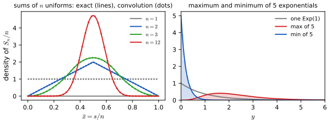
fig_2_s5. Illustrates Wasserman (2004), Example 2.48 and Exercises 2.7 and 2.21 (supplementary figure). Download: PDF · SVG2.13 Appendix
p. 43 A probability \(\P\) is defined on a \(\sigma\)-field \(\cA\) of subsets of \(\Omega\), and a random variable is a measurable map: \(\{\omega:X(\omega)\le x\}\in\cA\) for every \(x\). Filling the gap 2.1 shows that this one condition makes \(\P(X\in A)\) defined for every Borel set \(A\), and that the distribution \(P_X\) is a probability measure on \(\R\); Result 2.1 shows that \(P_X\) is determined by the cdf; and the proof of Result 2.2 shows that every cdf arises from a random variable on \(\Omega=(0,1)\). The same holds for random vectors, with half-lines replaced by the "south-west quadrants" \(\{y\in\R^k:y\le x\}\) (coordinatewise) and the cdf by the joint cdf.
Notes on the book
Six entries of the author's errata lists concern this chapter (collected in the first four boxes; two of them change a formula), and three more places need a more careful reading. Each was checked numerically.
Page 27, line 2: the geometric sum needs the exponent \(k-1\) (listed in the author's errata)
The display checking that the geometric mass function sums to one prints \(p\sum_{k\ge1}(1-p)^k\), which equals \(p(1-p)/p=1-p\), not 1. With the exponent \(k-1\) of the mass function the sum is \(p/(1-(1-p))=1\) (Result 2.6(a)). For \(p=0.3\): the printed sum is \(0.7\), the corrected one \(1\).
Page 30: the \(t\) density is missing the factor \(1/\sqrt{\nu\pi}\) (listed in the author's errata)
As printed, \(\frac{\Gamma((\nu+1)/2)}{\Gamma(\nu/2)}(1+x^2/\nu)^{-(\nu+1)/2}\) integrates to \(\sqrt{\nu\pi}\), not 1 (Result 2.9: for \(\nu=3\), numerically \(3.0700=\sqrt{3\pi}\)). The correct density divides by \(\sqrt{\nu\pi}\); for \(\nu=1\) this gives the Cauchy density \(1/(\pi(1+x^2))\) stated a few lines later.
Pages 26–27: binomial and Poisson sums need independence (listed in the author's errata)
"If \(X_1\sim\Bin(n_1,p)\) and \(X_2\sim\Bin(n_2,p)\) then \(X_1+X_2\sim\Bin(n_1+n_2,p)\)" requires \(X_1\ind X_2\), and so does the Poisson statement on page 27. With \(X_2=X_1\), the sum takes only even values. The same tacit assumption is spelled out for the Normal and gamma sums (pages 28 and 30). Also listed in the errata: on page 26 the \(k\) of the discrete uniform is an integer.
Page 29, line 1: there is no Normal table in the book (listed in the author's errata)
Example 2.17 and Exercise 2.18 refer to "the Normal table". The values used here come from \(\Phi\) and \(\Phi^{-1}\) computed numerically (scipy.stats.norm).
Page 25, Definition 2.16: the end points and the convention
With \(F^{-1}(q)=\inf\{x:F(x)\gt q\}\), \(F^{-1}(1)=\inf\emptyset=+\infty\), and \(F^{-1}(0)=-\infty\) for a law unbounded below (the Normal), so the quantile function is real-valued only on \((0,1)\); the statement that \(F^{-1}(q)\) is "the unique real number \(x\) such that \(F(x)=q\)" for strictly increasing continuous \(F\) holds for \(0\lt q\lt1\). The book's strict inequality also differs from the convention \(\inf\{x:F(x)\ge q\}\) used by most software: for two fair tosses the book's first quartile is \(F^{-1}(\tfrac14)=1\), the other one 0 (Definition 2.5).
Page 23: "\(f_X(x)=F_X'(x)\) at all points at which \(F_X\) is differentiable" holds almost everywhere
A density can be changed at a point without changing the distribution, so the identity can fail at individual points (the Uniform(0, 1) density redefined as 7 at \(x=\tfrac12\)). It holds at continuity points of \(f_X\), and for almost every \(x\) in general (Filling the gap 2.2). Relatedly, "continuous random variable" in Definition 2.11 means a cdf with a density (absolutely continuous), which is more than a continuous cdf: the Cantor distribution has a continuous cdf and no density.
Page 36, Theorem 2.33: the factorisation must include the support
"If \(f(x,y)=g(x)h(y)\)" must hold on the whole plane, indicator of the support included; that is what forces the support to be a rectangle. The density \(\frac{21}4x^2y\) of Example 2.28 is a product of a function of \(x\) and a function of \(y\) inside its support, but its support \(x^2\le y\le1\) is not a rectangle and \(X,Y\) are dependent (Result 2.12).
2.14 Exercises
All 21 exercises of Chapter 2 (Wasserman, 2004, pp. 43–46), restated in my own words, with complete solutions (hidden).
Exercise 2.1. Show that \(\P(X=x)=F(x+)-F(x-)\).
Solution
\(\{X\le x-1/n\}\uparrow\{X\lt x\}\), so continuity from below gives \(\P(X\lt x)=\lim_nF(x-1/n)=F(x-)\) (the limit exists and equals the left limit because \(F\) is monotone). Hence \(\P(X=x)=\P(X\le x)-\P(X\lt x)\)
\({}=F(x)-F(x-)\), and \(F(x)=F(x+)\) by right-continuity (Result 2.2). See Result 2.3. Exercise 2.2. \(X\) takes the values 2 and 3 with probability \(\tfrac1{10}\) each and 5 with probability \(\tfrac8{10}\). Plot its cdf and use it to find \(\P(2\lt X\le4.8)\) and \(\P(2\le X\le4.8)\).
Solution
\(F(x)=0\) for \(x\lt2\), \(0.1\) on \([2,3)\), \(0.2\) on \([3,5)\) and 1 for \(x\ge5\) (Figure 2.S1). By Result 2.3, \(\P(2\lt X\le4.8)=F(4.8)-F(2)\)
\({}=0.2-0.1=0.1\) and \(\P(2\le X\le4.8)=F(4.8)-F(2-)\) \({}=0.2-0=0.2\). The two answers differ by the jump at 2, which the closed interval includes. 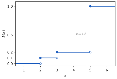
Figure 2.S1. The cdf of Exercise 2.2, with \(x=4.8\) marked. Code: fig_2_s1. Solves Wasserman (2004), Exercise 2.2 (supplementary figure). Download: PDF · SVGExercise 2.3. Prove Lemma 2.15.
Solution
This is Result 2.3, proved there: item 1 by continuity from below, items 2–3 by additivity, item 4 because a continuous random variable puts probability 0 on every point.
Exercise 2.4. \(X\) has density \(\tfrac14\) on \((0,1)\), \(\tfrac38\) on \((3,5)\) and 0 elsewhere. (a) Find its cdf. (b) Find the density of \(Y=1/X\) (consider \(\tfrac15\le y\le\tfrac13\), \(\tfrac13\le y\le1\) and \(y\ge1\)).
Solution
(a) \(F(x)=0\) for \(x\le0\); \(x/4\) for \(0\lt x\lt1\); \(\tfrac14\) for \(1\le x\le3\); \(\tfrac14+\tfrac38(x-3)\) for \(3\lt x\lt5\); 1 for \(x\ge5\).
(b) \(Y\) takes values in \((\tfrac15,\tfrac13)\cup(1,\infty)\). For \(y\gt0\), \(\P(Y\le y)=\P(X\ge1/y)=1-F(1/y)\). If \(y\ge1\), \(1/y\in(0,1]\) and \(F_Y(y)=1-\frac1{4y}\). If \(\tfrac13\le y\le1\), \(1/y\in[1,3]\) and \(F_Y(y)=\tfrac34\) (constant). If \(\tfrac15\le y\le\tfrac13\), \(1/y\in[3,5]\) and \(F_Y(y)=1-\tfrac14-\tfrac38(\tfrac1y-3)=\tfrac{15}8-\tfrac3{8y}\), which is 0 at \(y=\tfrac15\) and \(\tfrac34\) at \(y=\tfrac13\). Differentiating,
\[ f_Y(y)=\begin{cases}\dfrac{3}{8y^2}&\tfrac15\lt y\lt\tfrac13,\\[4pt] \dfrac1{4y^2}&y\gt1,\\[4pt] 0&\text{otherwise,}\end{cases} \]which is also what (2.12) gives directly, \(f_X(1/y)/y^2\). The two pieces carry probability \(\tfrac34\) and \(\tfrac14\). Figure 2.S2 (right) compares this with a simulation.
▶ DemoExercise 2.4(b) in the transformation demonstrationAt \(y=\tfrac14\): \(F_Y=\tfrac38\), and the preimage \(x=4\) gives \(f_Y=\tfrac38\times16=6\).Exercise 2.5. Show that discrete \(X\) and \(Y\) are independent if and only if \(f_{X,Y}(x,y)=f_X(x)f_Y(y)\) for all \(x,y\).
Solution
Result 2.11(a): one direction takes singletons in (2.7), the other sums the factorised mass function over \(A\times B\).
Exercise 2.6. \(X\) has density \(f\), \(A\subset\R\), and \(Y=\one_A(X)\). Find the cdf of \(Y\).
Solution
\(Y\) takes the values 1 (when \(X\in A\)) and 0, so it is \(\Bern(p)\) with \(p=\P(X\in A)=\int_Af(x)\,\d x\). Its cdf is \(F_Y(y)=0\) for \(y\lt0\), \(1-p\) for \(0\le y\lt1\), and 1 for \(y\ge1\).
Exercise 2.7. \(X,Y\) are independent \(\Unif(0,1)\) and \(Z=\min\{X,Y\}\). Find \(f_Z\).
Solution
For \(0\le z\le1\), \(\P(Z\gt z)=\P(X\gt z)\P(Y\gt z)\)
\({}=(1-z)^2\), so \(F_Z(z)=1-(1-z)^2\) and \(f_Z(z)=2(1-z)\) on \([0,1]\) (Result 2.21). A simulation of \(2\times10^5\) pairs agrees. Exercise 2.8. \(X\) has cdf \(F\). Find the cdf of \(X^+=\max\{0,X\}\).
Solution
\(X^+\ge0\), so \(F_{X^+}(x)=0\) for \(x\lt0\). For \(x\ge0\), \(\{X^+\le x\}=\{X\le x\}\), so \(F_{X^+}(x)=F(x)\). The law of \(X^+\) has an atom of size \(F(0)\) at 0 (all of \(X\)'s mass on \((-\infty,0]\) is moved there) and agrees with \(X\) on \((0,\infty)\): a mixed distribution, neither discrete nor continuous. The inverse-cdf demonstration samples it with \(X\sim\N(\mu,1)\).
Exercise 2.9. For \(X\sim\Exp(\beta)\), find \(F(x)\) and \(F^{-1}(q)\).
Solution
\(F(x)=\int_0^x\beta^{-1}e^{-t/\beta}\d t=1-e^{-x/\beta}\) for \(x\ge0\) (0 for \(x\lt0\)). Solving \(1-e^{-x/\beta}=q\) gives \(F^{-1}(q)=-\beta\log(1-q)\) for \(0\lt q\lt1\) (with \(F^{-1}(0)=0\) and \(F^{-1}(1)=\infty\)). The median is \(\beta\log2\).
Exercise 2.10. Show that if \(X\ind Y\), then \(g(X)\ind h(Y)\).
Solution
Result 2.13(a): \(\{g(X)\in A\}=\{X\in g^{-1}(A)\}\), and independence applies to the preimages.
Exercise 2.11. A coin with \(\P(\text{heads})=p\) is tossed. (a) With one toss, let \(X\) and \(Y\) be the numbers of heads and tails; show that they are dependent. (b) With \(N\sim\Poi(\lambda)\) tosses, show that the numbers of heads and tails are independent.
Solution
(a) \(X+Y=1\). For \(0\lt p\lt1\), \(\P(X=1,Y=1)=0\) but \(\P(X=1)\P(Y=1)=p(1-p)\gt0\). (For \(p\in\{0,1\}\) both are constants, and constants are independent of everything.)
(b) Given \(N=n\), \(X\sim\Bin(n,p)\) and \(Y=n-X\). With \(q=1-p\),
\[ \P(X=x,Y=y)=\P(N=x+y)\binom{x+y}xp^xq^y=e^{-\lambda}\frac{\lambda^{x+y}}{(x+y)!}\frac{(x+y)!}{x!\,y!}p^xq^y=e^{-\lambda p}\frac{(\lambda p)^x}{x!}\cdot e^{-\lambda q}\frac{(\lambda q)^y}{y!}, \]using \(e^{-\lambda}=e^{-\lambda p}e^{-\lambda q}\). The joint mass function factorises, so \(X\sim\Poi(\lambda p)\) and \(Y\sim\Poi(\lambda q)\) are independent (Result 2.11(a)). This is "Poisson thinning": randomising the number of trials removes the constraint \(X+Y=n\).
Exercise 2.12. Prove Theorem 2.33.
Solution
Result 2.12: with \(G=\int g\), \(H=\int h\), \(GH=1\), \(f_X=gH\), \(f_Y=Gh\), so \(f_Xf_Y=f\). The proof there also explains why the support must be a rectangle.
Exercise 2.13. \(X\sim\N(0,1)\), \(Y=e^X\). (a) Find and plot the density of \(Y\). (b) Simulate 10,000 values \(e^{x_i}\) and compare their histogram with (a).
Solution
(a) \(r(x)=e^x\) is increasing with inverse \(s(y)=\log y\), \(s'(y)=1/y\), so by (2.12)
\[ f_Y(y)=\frac{1}{y\sqrt{2\pi}}e^{-(\log y)^2/2},\qquad y\gt0, \]the log-normal density; it is 0 at \(y=0^+\), peaks at \(y=e^{-1}\) and has a long right tail; its median is 1.
(b) Figure 2.S3 (code
fig_2_s3, seed 213): the histogram of the 10,000 simulated values follows the curve; a Kolmogorov–Smirnov comparison with the log-normal law shows no discrepancy. Try preset 3 of the transformation demonstration.Exercise 2.14. \((X,Y)\) is uniform on the unit disk and \(R=\sqrt{X^2+Y^2}\). Find the cdf and density of \(R\).
Solution
The joint density is \(1/\pi\) on the disk. For \(0\le r\le1\), \(\{R\le r\}\) is the disk of radius \(r\), of area \(\pi r^2\), so \(F_R(r)=r^2\) and \(f_R(r)=2r\) on \([0,1]\) (with \(F_R=0\) below 0 and 1 above 1). Points near the rim are more likely than points near the centre because there is more area there.
Exercise 2.15. (Probability integral transform.) Let \(X\) have a continuous, strictly increasing cdf \(F\) and \(Y=F(X)\): find the density of \(Y\). Let \(U\sim\Unif(0,1)\) and \(X=F^{-1}(U)\): show \(X\sim F\). Write a program that turns uniforms into \(\Exp(\beta)\) variables.
Solution
By Result 2.4: \(\P(F(X)\le y)=\P(X\le F^{-1}(y))\)
\({}=F(F^{-1}(y))=y\) for \(0\lt y\lt1\), so \(Y\sim\Unif(0,1)\), density 1 on \((0,1)\); and \(\P(F^{-1}(U)\le x)=\P(U\le F(x))=F(x)\). (Result 2.4 proves both without assuming \(F\) strictly increasing, and the second for any cdf.) The program, with Exercise 2.9: import numpy as np def exp_from_uniform(u, beta): """X = F^{-1}(U) = -beta log(1 - U) is Exp(beta) when U is Uniform(0, 1).""" return -beta * np.log1p(-u) x = exp_from_uniform(np.random.default_rng(0).uniform(size=10000), beta=2.0)Figure 2.S4 shows 10,000 such draws against the \(\Exp(2)\) density; their mean is 2.03 against \(\beta=2\) (the standard error of the mean of 10,000 draws is \(\beta/100=0.02\)). (\(-\beta\log U\) works equally well, since \(1-U\) is also uniform.)
Exercise 2.16. \(X\sim\Poi(\lambda)\) and \(Y\sim\Poi(\mu)\) are independent. Show that \(X\given X+Y=n\sim\Bin(n,\pi)\) with \(\pi=\lambda/(\lambda+\mu)\).
Solution
\(X+Y\sim\Poi(\lambda+\mu)\) (Result 2.6(c)) and \(\{X=x,X+Y=n\}\)
\[ \P(X=x\given X+Y=n)=\frac{e^{-\lambda}\frac{\lambda^x}{x!}\,e^{-\mu}\frac{\mu^{n-x}}{(n-x)!}}{e^{-(\lambda+\mu)}\frac{(\lambda+\mu)^n}{n!}}=\binom nx\Big(\frac\lambda{\lambda+\mu}\Big)^x\Big(\frac\mu{\lambda+\mu}\Big)^{n-x}. \]\({}=\{X=x,Y=n-x\}\), so for \(0\le x\le n\) Exercise 2.17. \(f_{X,Y}(x,y)=c(x+y^2)\) on the unit square. Find \(\P(X\lt\tfrac12\given Y=\tfrac12)\).
Solution
\(\iint(x+y^2)=\tfrac12+\tfrac13=\tfrac56\), so \(c=\tfrac65\). \(f_Y(\tfrac12)=c\int_0^1(x+\tfrac14)\d x=\tfrac34c\), so \(f_{X\given Y}(x\given\tfrac12)=(x+\tfrac14)/\tfrac34\) on \([0,1]\) (the constant \(c\) cancels), and
\[ \P\big(X\lt\tfrac12\given Y=\tfrac12\big)=\frac43\int_0^{1/2}\Big(x+\frac14\Big)\d x=\frac43\Big(\frac18+\frac18\Big)=\frac13. \]Exercise 2.18. \(X\sim\N(3,16)\). Find (a) \(\P(X\lt7)\); (b) \(\P(X\gt-2)\); (c) \(x\) with \(\P(X\gt x)=0.05\); (d) \(\P(0\le X\lt4)\); (e) \(x\) with \(\P(|X|\gt|x|)=0.05\).
Solution
Here \(\sigma=4\) and \(Z=(X-3)/4\). (a) \(\Phi(1)=0.8413\). (b) \(1-\Phi(-1.25)=\Phi(1.25)=0.8944\). (c) \(x=3+4\Phi^{-1}(0.95)=3+4(1.6449)\)
\[ \P(X\gt c)+\P(X\lt-c)=1-\Phi\Big(\frac{c-3}4\Big)+\Phi\Big(\frac{-c-3}4\Big)=0.05. \]\({}=9.5794\). (d) \(\Phi(0.25)-\Phi(-0.75)\) \({}=0.5987-0.2266=0.3721\). (e) With \(c=|x|\), solve Because \(X\) is not centred at 0 the two tails are unequal and there is no closed form; numerically \(c=9.611\) (tails 0.0492 and 0.0008), so \(x=\pm9.611\). The tempting \(3+1.96\times4=10.84\) answers a different question, \(\P(|X-3|\gt x-3)=0.05\). (Computed with
scipy.stats.norm, since the book has no Normal table.)Exercise 2.19. Prove formula (2.12).
Solution
Result 2.17(a): for increasing \(r\), \(F_Y(y)=F_X(s(y))=\int^{s(y)}f_X\), and the substitution \(x=s(t)\) exhibits \(f_X(s(t))s'(t)\) as a density of \(Y\); for decreasing \(r\) the same with \(-s'=|s'|\).
Exercise 2.20. \(X,Y\) independent \(\Unif(0,1)\). Find the densities of \(X-Y\) and \(X/Y\).
Solution
\(X-Y=X+(-Y)\) with \(-Y\sim\Unif(-1,0)\), so by the convolution formula \(f_{X-Y}(z)\) is the length of \([0,1]\cap[z,z+1]\), which is \(1-|z|\) for \(|z|\le1\) and 0 otherwise (a triangle on \([-1,1]\)).
For the ratio (Filling the gap 2.4), \(f_{X/Y}(z)=\int_0^1y\,\one\{zy\lt1\}\,\d y\): for \(0\lt z\le1\) this is \(\int_0^1y\,\d y=\tfrac12\), and for \(z\gt1\) it is \(\int_0^{1/z}y\,\d y=\frac1{2z^2}\). Check: \(\tfrac12+\int_1^\infty\frac{\d z}{2z^2}=1\). Directly: \(\P(X/Y\le z)\) is the area of \(\{x\le zy\}\) in the square, \(z/2\) for \(z\le1\) and \(1-\frac1{2z}\) for \(z\gt1\). Both answers agree with simulations of \(2\times10^5\) pairs.
Exercise 2.21. \(X_1,\dots,X_n\iid\Exp(\beta)\) and \(Y=\max_iX_i\). Find the density of \(Y\).
Solution
\(Y\le y\) exactly when every \(X_i\le y\), so \(F_Y(y)=(1-e^{-y/\beta})^n\) for \(y\ge0\) and
\[ f_Y(y)=\frac n\beta\big(1-e^{-y/\beta}\big)^{n-1}e^{-y/\beta},\qquad y\gt0 \](Result 2.21; Figure 2.S5 shows \(n=5\)).
Demonstrations for this chapter
Each demonstration runs in the browser and links back to these notes. The ▶ Demo boxes above open them already set to the case under discussion.
| Demonstration | What you can see | Sections and results |
|---|---|---|
| Inverse-cdf sampling | Uniforms pushed through the quantile function of nine laws (exponential, Normal, Cauchy, two coin flips, Poisson, geometric, the mixed law \(\max(0,X)\), the nerve data of the book's website and an exponential fitted to them): the path \(u\to F^{-1}(u)\), the draws against the target, the largest cdf gap \(D_n\), and the two conventions for \(F^{-1}\). Presets: 1 Exp(1); 2 the staircase of Example 2.6; 3 Poisson(3); 4 a mixed law; 5 the empirical cdf (the bootstrap). | 2.2; Definition 2.5, Result 2.4, Exercise 2.15 |
| Transformations by the cdf method | Four laws of \(X\) and six maps (\(x^2\), \(|x|\), \(e^x\), \(\log x\), \(1/x\), \(F_X(x)\)): the set \(A_y\), the area \(F_Y(y)\), and \(f_Y\) as a sum of one band per preimage branch, over a histogram of simulated values. Presets: 1 Example 2.47; 2 Example 2.46; 3 Exercise 2.13; 4 the probability integral transform; 5 Exercise 2.4(b). | 2.11; Result 2.17, 2.10, 2.4 |
| The distribution of a sum | Sums of up to 30 independent uniform, exponential, Normal, Cauchy, Bernoulli or Poisson terms by repeated convolution: flip and slide, the plane picture of \(\P(S_n\le z)\), the exact law, the Normal approximation and 5000 simulated sums. Presets: 1 Example 2.48; 2 twelve uniforms; 3 exponentials and the gamma; 4 Poissons; 5 Cauchys. | 2.12; Results 2.19, 2.20 |
Related demonstrations: in the companion courses, the basic sampling algorithms of Bayesian and Probabilistic Machine Learning (the transformation method and Box–Muller) and the change-of-variables demo of Foundations of Deep Learning (the moving mode and the two-dimensional Jacobian). The Python code that produces every figure of this page is code/ch02_random_variables.py (see the code index).
References
- Wasserman, L. (2004). All of Statistics: A Concise Course in Statistical Inference. Springer, New York. Chapter 2, pp. 19–46. www.stat.cmu.edu/~larry/all-of-statistics.
- Billingsley, P. (1995). Probability and Measure, 3rd edition. Wiley, New York. (Distribution functions, the \(\pi\)–\(\lambda\) theorem, Lebesgue's decomposition, change of variables.)
- Box, G. E. P. and Muller, M. E. (1958). A note on the generation of random normal deviates. The Annals of Mathematical Statistics, 29(2), 610–611.
- Casella, G. and Berger, R. L. (2002). Statistical Inference, 2nd edition. Duxbury, Pacific Grove. Chapters 2–5 (transformations, multiple random variables, order statistics).
- Cox, D. R. and Lewis, P. A. W. (1966). The Statistical Analysis of Series of Events. Methuen, London. (The nerve pulse data.)
- DeGroot, M. H. and Schervish, M. J. (2002). Probability and Statistics, 3rd edition. Addison-Wesley, Boston. (Example 2.22 is taken from this book.)
- Devroye, L. (1986). Non-Uniform Random Variate Generation. Springer, New York. (The inversion method and its relatives.)
- Feller, W. (1971). An Introduction to Probability Theory and Its Applications, Volume II, 2nd edition. Wiley, New York. (Convolutions, the Cauchy and stable laws.)
- Hall, P. (1927). The distribution of means for samples of size N drawn from a population in which the variate takes values between 0 and 1, all such values being equally probable. Biometrika, 19(3/4), 240–245.
- Irwin, J. O. (1927). On the frequency distribution of the means of samples from a population having any law of frequency with finite moments, with special reference to Pearson's Type II. Biometrika, 19(3/4), 225–239.
- Scheffé, H. (1947). A useful convergence theorem for probability distributions. The Annals of Mathematical Statistics, 18(3), 434–438.
The numerical statements in the text (the values in the examples and exercises, the normalising constants, the closure of the families under sums, the factorisation criteria, the multivariate Normal identities, the transformation and convolution formulas, the laws of the maximum and the minimum, and the corrections listed in the notes on the book) were confirmed numerically.