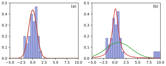
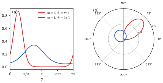
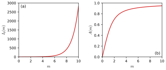
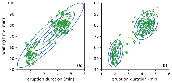
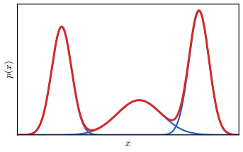
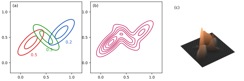
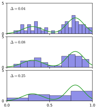
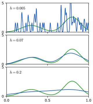
Every later chapter is built from a small stock of distributions, and this chapter supplies it. It starts with the distributions of discrete data (Bernoulli, binomial, multinomial) together with their conjugate priors (beta, Dirichlet), which show Bayesian learning in its simplest form: the prior acts as a set of pseudo-observations and the posterior is a compromise between prior and data. It then studies the Gaussian in depth (its geometry, its conditionals and marginals, Bayes' theorem for linear-Gaussian models, maximum likelihood, sequential estimation, conjugate Bayesian inference, the Student t as a mixture of Gaussians, the von Mises distribution for angles, and mixtures), unifies the examples in the exponential family, and ends with the density estimators that do not assume a parametric form: histograms, kernels and nearest neighbours. Every step the book leaves to the reader is written out below, and all 61 exercises are solved.
They follow the book. Sections carry Bishop's numbers (2.1, 2.3.6, ...) and every displayed equation that appears in the book carries the book's own equation number, e.g. (2.43), so you can read these notes next to the book. Equations without a number are steps that the book skips.
Filling the gaps. Wherever the book says that a result "can be shown", is "easily verified", or is left as an exercise, an orange Filling the gap box or a proof gives the full argument. Proofs and derivations start hidden: open one with its bar, or use the button below.
Figures and demonstrations. The numerical figures of the chapter are reproduced from scratch by the Python code. The ▶ Demo boxes open an interactive demonstration already set to the case being discussed. Gaussian identities (completing the square, the linear-Gaussian model, the Woodbury identity), the exponential-family moments and the gamma, Dirichlet, Wishart and Student t distributions are proved in the mathematical toolkit; here they are linked, and only what the toolkit lacks is added.
Main reference
C. M. Bishop, Pattern Recognition and Machine Learning, Springer (2006), Chapter 2, pages 67–136. Section, equation, figure and exercise numbers below refer to this book. Further reading is listed in the references.
The explanations, derivations and code are my own; equations are cited by their numbers in the book.
The chapter at a glance
2.1–2.2 Counts of a binary or \(K\)-state variable have the likelihood \(\prod_k\mu_k^{m_k}\). Maximum likelihood returns the empirical frequencies (and over-fits small samples); a beta or Dirichlet prior has the same functional form, so the posterior is again beta or Dirichlet with the counts added to the prior parameters.
2.3 The Gaussian is determined by its mean and covariance; its contours are ellipsoids along the eigenvectors of the covariance. Conditionals, marginals and linear-Gaussian models stay Gaussian. For the mean with known precision the Gaussian prior is conjugate, for the precision a gamma, and jointly a Gaussian-gamma (Gaussian-Wishart). Integrating out an unknown precision turns the Gaussian into a heavy-tailed Student t. Angles need the von Mises distribution; multimodal data need mixtures.
2.4 Most of these distributions are members of one family, \(p(\mathbf{x}\given\bm\eta)\)\({}=h(\mathbf{x})g(\bm\eta)\exp\{\bm\eta^\T\mathbf{u}(\mathbf{x})\}\), whose maximum likelihood estimate depends on the data only through \(\sum_n\mathbf{u}(\mathbf{x}_n)\), and which always has a conjugate prior. Location and scale parameters get the non-informative priors \(p(\mu)\propto 1\) and \(p(\sigma)\propto1/\sigma\).
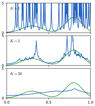
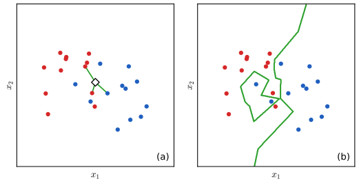
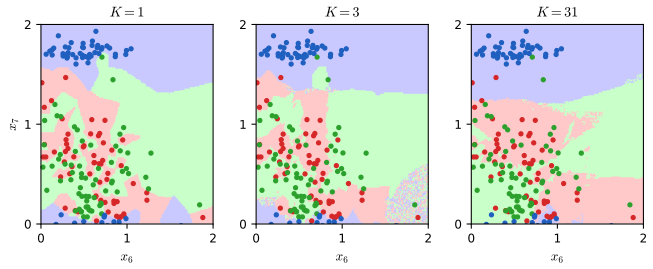
2.5 Without a parametric form, the density at \(\mathbf{x}\) is estimated from the number \(K\) of points in a small region of volume \(V\) as \(K/(NV)\): fix \(V\) (histograms, kernels) or fix \(K\) (nearest neighbours). The latter also gives a classifier whose error is at most twice the Bayes error.
Notation. Data \(\mathcal{D}=\{x_1,\dots,x_N\}\) (or \(\mathbf{X}\) for vectors); \(\mu\) is a probability in Sections 2.1–2.2 and a mean in 2.3, as in the book; \(\bm\Lambda=\bm\Sigma^{-1}\) is the precision matrix and \(\lambda=1/\sigma^2\) the scalar precision (the book also writes \(\tau\) in Section 2.3.7). \(\Gamma\) is the gamma function and \(\psi=\Gamma'/\Gamma\) the digamma function.
Prerequisites. Probability rules, expectation and variance, and the entropy and KL divergence of Chapter 1; basic linear algebra (eigenvalues, determinants, trace); Lagrange multipliers (toolkit).
Printings. The text used here is a corrected printing. Where Bishop's errata list corrects an equation of this chapter, the notes give the corrected form and a short Erratum note naming the original.
Derivations start hidden: click any bar to open one.
2.1 Binary variables
pp. 68–74 The simplest random variable takes two values, such as the outcome of a coin flip, \(x\in\{0,1\}\). Its law is fixed by one number, the probability of heads, and the whole Bayesian machinery (likelihood, prior, posterior, predictive distribution) can be carried out in closed form. Everything later in the chapter is a generalisation of what is done here.
Definition 2.1 (Bernoulli and binomial distributions) pp. 68–70, (2.1)–(2.4), (2.9)–(2.12)
With \(p(x=1\given\mu)=\mu\), \(0\le\mu\le1\), the Bernoulli distribution is
Result 2.1 (the Bernoulli and binomial distributions: normalisation, mean, variance, entropy) (2.257)–(2.264), (2.11), (2.12); Exercises 2.1, 2.3, 2.4
(a) \(\sum_{x\in\{0,1\}}p(x\given\mu)=1\), \(\E[x]=\mu\), \(\var[x]=\mu(1-\mu)\), and the entropy is \(\mathrm H[x]=-\mu\ln\mu-(1-\mu)\ln(1-\mu)\). (b) \(\sum_{m=0}^{N}\mathrm{Bin}(m\given N,\mu)=1\), \(\E[m]=N\mu\) and \(\var[m]=N\mu(1-\mu)\).
Proof
(a) \(p(0\given\mu)+p(1\given\mu)=(1-\mu)+\mu=1\). \(\E[x]=0\cdot(1-\mu)+1\cdot\mu=\mu\); since \(x^2=x\), \(\E[x^2]=\mu\) and \(\var[x]=\mu-\mu^2\). The entropy is \(-\sum_xp(x)\ln p(x)\)\({}=-(1-\mu)\ln(1-\mu)-\mu\ln\mu\). (It is largest, \(\ln2\), at \(\mu=\tfrac12\) and zero at \(\mu\in\{0,1\}\).)
(b) Pascal's rule. For \(1\le m\le N\), \(\binom Nm+\binom N{m-1}\)\({}=\frac{N!}{m!(N-m)!}+\frac{N!}{(m-1)!(N-m+1)!}\)\({}=\frac{N!\,[(N-m+1)+m]}{m!\,(N-m+1)!}\)\({}=\binom{N+1}{m}\).
Binomial theorem, \((1+x)^N=\sum_{m=0}^N\binom Nmx^m\) for all real \(x\), by induction on \(N\). For \(N=1\) both sides are \(1+x\). If it holds for \(N\), then, shifting the index in the second sum and using \(\binom N{-1}=\binom N{N+1}=0\),
\[ (1+x)^{N+1}=\sum_{m=0}^N\binom Nmx^m+\sum_{m=0}^N\binom Nmx^{m+1}=\sum_{m=0}^{N+1}\Big[\binom Nm+\binom N{m-1}\Big]x^m=\sum_{m=0}^{N+1}\binom{N+1}mx^m. \]
Normalisation. Pull out \((1-\mu)^N\): \(\sum_m\binom Nm\mu^m(1-\mu)^{N-m}\)\({}=(1-\mu)^N\sum_m\binom Nm\big(\tfrac{\mu}{1-\mu}\big)^m\)\({}=(1-\mu)^N\big(1+\tfrac{\mu}{1-\mu}\big)^N\)\({}=1\) (for \(\mu<1\); at \(\mu=1\) the sum is \(1\) trivially).
Mean and variance. For \(0<\mu<1\), \(\frac{\partial}{\partial\mu}\ln\mathrm{Bin}(m\given N,\mu)\)\({}=\frac m\mu-\frac{N-m}{1-\mu}\)\({}=\frac{m-N\mu}{\mu(1-\mu)}\), so \(\partial_\mu\mathrm{Bin}\)\({}=\mathrm{Bin}\cdot\frac{m-N\mu}{\mu(1-\mu)}\). Differentiate the normalisation \(\sum_m\mathrm{Bin}(m\given N,\mu)=1\):
\[ 0=\sum_m\frac{m-N\mu}{\mu(1-\mu)}\mathrm{Bin}(m\given N,\mu)\ \Rightarrow\ \E[m]=N\mu. \]
Differentiate once more the identity \(\sum_m(m-N\mu)\mathrm{Bin}=0\) (which is what we just proved):
\[ 0=\sum_m\big[-N\,\mathrm{Bin}+(m-N\mu)\,\partial_\mu\mathrm{Bin}\big]=-N+\frac{1}{\mu(1-\mu)}\sum_m(m-N\mu)^2\mathrm{Bin}, \]
so \(\var[m]=N\mu(1-\mu)\). (Alternatively, \(m\) is a sum of \(N\) independent Bernoulli variables: means and variances add, Exercise 1.10.) ∎
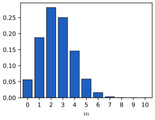
Figure 2.1 (reproduced). The binomial distribution \(\mathrm{Bin}(m\given 10,0.25)\); mean \(N\mu=2.5\), variance \(N\mu(1-\mu)=1.875\). Book: Figure 2.1, p. 70. Code: ch02_probability_distributions.py, fig2_1. Download: PDF · SVG
Maximum likelihood and its over-fitting
pp. 68–69 Given i.i.d. observations \(\mathcal{D}=\{x_1,\dots,x_N\}\), the likelihood and log likelihood of the Bernoulli model are
The data enter only through \(\sum_nx_n\), the first example of a sufficient statistic (Section 2.4.1). Setting the derivative to zero, \(\sum_n\big[\frac{x_n}{\mu}-\frac{1-x_n}{1-\mu}\big]\)\({}=0\), i.e. \(\sum_n(x_n-\mu)=0\), gives the sample proportion
It is a maximum because \(\frac{\partial^2}{\partial\mu^2}\ln p\)\({}=-\sum_n\big[\frac{x_n}{\mu^2}+\frac{1-x_n}{(1-\mu)^2}\big]<0\). The weakness: for a small sample the estimate is extreme. With \(N=m=3\) heads, \(\mu_{\rm ML}=1\), and the model forecasts that every future flip will be heads. A prior distribution over \(\mu\) removes this pathology.
2.1.1 The beta distribution
pp. 71–74 The likelihood is proportional to \(\mu^m(1-\mu)^{N-m}\), a product of a power of \(\mu\) and a power of \(1-\mu\). A prior of the same form is therefore conjugate: the posterior, being prior times likelihood, has the same form again. The beta distribution is the normalised version
Normalisation. From \(\Gamma(a)=\int_0^\infty e^{-x}x^{a-1}\d x\) (1.141),
\[ \Gamma(a)\Gamma(b)=\int_0^\infty\!\!\int_0^\infty e^{-x-y}x^{a-1}y^{b-1}\,\d y\,\d x. \]
Fix \(x\) and substitute \(t=x+y\) (so \(t\) runs from \(x\) to \(\infty\)): \(\Gamma(a)\Gamma(b)\)\({}=\int_0^\infty\!\int_x^\infty e^{-t}x^{a-1}(t-x)^{b-1}\,\d t\,\d x\). The region is \(0\le x\le t<\infty\); exchange the order of integration (everything is non-negative, so Tonelli applies): \(=\int_0^\infty e^{-t}\int_0^tx^{a-1}(t-x)^{b-1}\,\d x\,\d t\). In the inner integral put \(x=t\mu\), \(\d x=t\,\d\mu\): it becomes \(t^{a+b-1}\int_0^1\mu^{a-1}(1-\mu)^{b-1}\d\mu\). Hence
\[ \Gamma(a)\Gamma(b)=\int_0^\infty e^{-t}t^{a+b-1}\d t\int_0^1\mu^{a-1}(1-\mu)^{b-1}\d\mu=\Gamma(a+b)\int_0^1\mu^{a-1}(1-\mu)^{b-1}\d\mu. \]
Moments. Write \(B(a,b)=\Gamma(a)\Gamma(b)/\Gamma(a+b)\). Then \(\E[\mu^k]=B(a+k,b)/B(a,b)\), and with \(\Gamma(x+1)=x\Gamma(x)\): \(\E[\mu]\)\({}=\frac{\Gamma(a+1)\Gamma(a+b)}{\Gamma(a)\Gamma(a+b+1)}\)\({}=\frac a{a+b}\), \(\E[\mu^2]=\frac{a(a+1)}{(a+b)(a+b+1)}\). Therefore
\[ \var[\mu]=\frac{a(a+1)}{(a+b)(a+b+1)}-\frac{a^2}{(a+b)^2}=\frac{a[(a+1)(a+b)-a(a+b+1)]}{(a+b)^2(a+b+1)}=\frac{ab}{(a+b)^2(a+b+1)}. \]
Mode. For \(a,b>1\) the log density \((a-1)\ln\mu+(b-1)\ln(1-\mu)\) is strictly concave, vanishing at the end points like \(-\infty\), with derivative \(\frac{a-1}{\mu}-\frac{b-1}{1-\mu}=0\) at \(\mu=\frac{a-1}{a+b-2}\). ∎
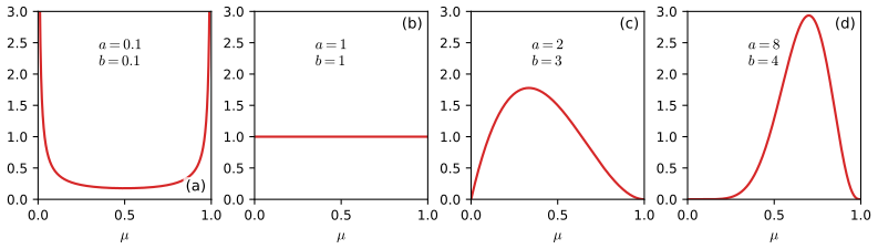
Figure 2.2 (reproduced). The beta density for four choices of \((a,b)\): \((0.1,0.1)\) piles mass at both ends, \((1,1)\) is uniform, \((2,3)\) and \((8,4)\) are unimodal with mode \((a-1)/(a+b-2)\); a larger \(a+b\) gives a narrower density. Book: Figure 2.2, p. 72. Code: ch02_probability_distributions.py, fig2_2. Download: PDF · SVG
▶ DemoBeta prior, one observation (Figure 2.2)Change \(a\) and \(b\) to see the shapes of Figure 2.2, then add a single observation and watch the posterior move.
Posterior. Multiplying the prior (2.13) by the binomial likelihood with \(m\) ones and \(l=N-m\) zeros, and keeping only factors that depend on \(\mu\),
So the prior parameters \(a\) and \(b\) act as an effective number of observations of \(x=1\) and \(x=0\) (they need not be integers). Observing one more data point simply increments \(a\) or \(b\) by one.
Result 2.3 (sequential Bayesian updating; posterior mean between prior mean and ML) pp. 72–73, Exercise 2.7
(a) Updating the beta posterior one observation at a time gives the same posterior as processing all data in one batch. (b) The posterior mean is a convex combination of the prior mean and the maximum likelihood estimate:
\[ \E[\mu\given\mathcal{D}]=\frac{m+a}{m+l+a+b}=\lambda\,\frac{a}{a+b}+(1-\lambda)\,\frac mN,\qquad\lambda=\frac{a+b}{N+a+b}\in(0,1]. \]
Proof
(a) Because the observations are independent given \(\mu\), the likelihood is the product of per-point factors \(\mu^{x_n}(1-\mu)^{1-x_n}\). Using the posterior after \(n-1\) points as the prior for the \(n\)-th multiplies in one factor, so after \(N\) points the posterior is prior times all \(N\) factors: the same as the batch posterior. For a beta prior each step maps \((a,b)\mapsto(a+1,b)\) if \(x_n=1\) and \((a,b+1)\) if \(x_n=0\), so the final parameters are \((a+m,b+l)\) regardless of order.
(b) \(\E[\mu\given\mathcal{D}]=\frac{a+m}{(a+m)+(b+l)}\) by (2.15) applied to (2.18). Write \(a+m=\frac{a}{a+b}(a+b)+\frac mN N\) and divide by \(N+a+b\). As \(N\to\infty\), \(\lambda\to0\) and the mean tends to \(\mu_{\rm ML}\). ∎
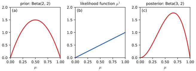
Figure 2.3 (reproduced). One step of sequential Bayesian inference: the prior \(\mathrm{Beta}(\mu\given2,2)\) (left), the likelihood \(\mu^{x}(1-\mu)^{1-x}\) of one observation \(x=1\) (centre) and the posterior \(\mathrm{Beta}(\mu\given3,2)\) (right). Book: Figure 2.3, p. 73. Code: ch02_probability_distributions.py, fig2_3. Download: PDF · SVG
For \(m,l\to\infty\) this tends to the maximum-likelihood prediction \(m/N\), a general feature of Bayesian inference. With \(a=b=1\) it is Laplace's "rule of succession" \((m+1)/(N+2)\); after three heads in three flips it predicts heads with probability \(4/5\), not \(1\).
Result 2.4 (conditional expectation and variance; Bayesian learning reduces uncertainty on average) (2.21)–(2.24), (2.270), (2.271); Exercise 2.8
For any two random variables, \(\E[x]=\E_y[\E_x[x\given y]]\) and \(\var[x]\)\({}=\E_y[\var_x[x\given y]]+\var_y[\E_x[x\given y]]\). Applied to a parameter \(\theta\) and a data set \(\mathcal{D}\) drawn from the model,
\[ \E_\theta[\theta]=\E_{\mathcal{D}}\big[\E_\theta[\theta\given\mathcal{D}]\big],\qquad \var_\theta[\theta]=\E_{\mathcal{D}}\big[\var_\theta[\theta\given\mathcal{D}]\big]+\var_{\mathcal{D}}\big[\E_\theta[\theta\given\mathcal{D}]\big]. \tag{2.21, 2.24} \]
Hence the posterior variance, averaged over data sets, is no larger than the prior variance. (A particular data set can make the posterior wider: Bayes' theorem only guarantees the average.)
Proof
\(\E_y[\E_x[x\given y]]\)\({}=\int\!\big(\int x\,p(x\given y)\,\d x\big)p(y)\,\d y\)\({}=\iint x\,p(x,y)\,\d x\,\d y\)\({}=\E[x]\). For the variance, \(\E[x^2]\)\({}=\E_y[\E_x[x^2\given y]]\)\({}=\E_y[\var_x[x\given y]+(\E_x[x\given y])^2]\), so
\[ \var[x]=\E_y[\var_x[x\given y]]+\E_y[(\E_x[x\given y])^2]-(\E_y[\E_x[x\given y]])^2=\E_y[\var_x[x\given y]]+\var_y[\E_x[x\given y]]. \]
Take \(x=\theta\) and \(y=\mathcal{D}\) (the joint is prior times likelihood). The last term is non-negative, so \(\E_{\mathcal{D}}[\var[\theta\given\mathcal{D}]]\)\({}\le\var[\theta]\). ∎
For the beta posterior, the variance in (2.16) with \((a,b)\to(a+m,b+l)\) is \(\frac{(a+m)(b+l)}{(a+b+N)^2(a+b+N+1)}\)\({}\le\frac{1}{4(a+b+N+1)}\), which falls like \(1/N\): the posterior concentrates.
2.2 Multinomial variables
pp. 74–78 A variable that takes one of \(K\) mutually exclusive states is coded in 1-of-\(K\) form: \(\mathbf{x}=(0,\dots,0,1,0,\dots,0)^\T\) with \(x_k=1\) if state \(k\) occurs, so \(\sum_kx_k=1\). If \(p(x_k=1)=\mu_k\), with \(\mu_k\ge0\) and \(\sum_k\mu_k=1\),
so the data enter only through the counts \(m_k\) (sufficient statistics).
Result 2.5 (maximum likelihood for the multinomial; the multinomial distribution) (2.31)–(2.37); Section 2.2
The maximiser of \(\prod_k\mu_k^{m_k}\) over the simplex is \(\mu_k^{\rm ML}=m_k/N\) (2.33). The joint distribution of the counts \((m_1,\dots,m_K)\) is the multinomial
\[ \mathrm{Mult}(m_1,\dots,m_K\given\bm\mu,N)=\frac{N!}{m_1!\,m_2!\cdots m_K!}\prod_{k=1}^K\mu_k^{m_k},\qquad\sum_km_k=N, \tag{2.34, 2.35} \]
and it sums to one.
Proof
Lagrange multiplier (toolkit). Maximise \(\sum_km_k\ln\mu_k\) subject to \(\sum_k\mu_k=1\) via
\[ \sum_{k=1}^Km_k\ln\mu_k+\lambda\Big(\sum_{k=1}^K\mu_k-1\Big).\tag{2.31} \]
Setting the derivative with respect to \(\mu_k\) to zero: \(m_k/\mu_k+\lambda=0\), i.e. \(\mu_k=-m_k/\lambda\) (2.32). Substituting in the constraint, \(-\sum_km_k/\lambda=1\), so \(\lambda=-N\) and \(\mu_k^{\rm ML}=m_k/N\). It is the global maximum because the objective is concave on the simplex (a sum of concave logarithms with non-negative weights) and the constraint is linear. (Also: for any other \(\bm\mu\), \(\sum_km_k\ln(\mu_k/\mu_k^{\rm ML})\)\({}\le N\ln\sum_k\mu^{\rm ML}_k\mu_k/\mu_k^{\rm ML}\)\({}=0\) by Jensen.)
Multinomial. For a fixed count vector the \(N\) observations can be assigned to the \(K\) states in \(N!/(m_1!\cdots m_K!)\) ways (choose which of the \(N\) data points go to state 1, then which of the remaining go to state 2, and so on, giving \(\binom N{m_1}\binom{N-m_1}{m_2}\cdots\)), each with probability \(\prod_k\mu_k^{m_k}\) by (2.29). Normalisation is the multinomial theorem \((\mu_1+\dots+\mu_K)^N\)\({}=\sum_{\sum m_k=N}\frac{N!}{\prod_km_k!}\prod_k\mu_k^{m_k}\), whose left side is \(1\): it follows by induction on \(K\) from the binomial theorem of Result 2.1, grouping the last \(K-1\) terms. ∎
2.2.1 The Dirichlet distribution
pp. 76–78 The conjugate prior for the multinomial has the same form as the likelihood, \(p(\bm\mu\given\bm\alpha)\)\({}\propto\prod_k\mu_k^{\alpha_k-1}\), on the simplex \(0\le\mu_k\le1\), \(\sum_k\mu_k=1\) (Figure 2.4, a \((K-1)\)-dimensional triangle for \(K=3\)). The normalised Dirichlet distribution is
Result 2.6 (the Dirichlet distribution: normalisation, moments, posterior) (2.38)–(2.41), (2.272)–(2.277); Exercises 2.9–2.11
(a) \(\displaystyle\int_{\rm simplex}\prod_k\mu_k^{\alpha_k-1}\,\d\bm\mu\)\({}=\frac{\prod_k\Gamma(\alpha_k)}{\Gamma(\alpha_0)}\), so (2.38) is normalised. (b) With \(\alpha_0=\sum_k\alpha_k\),
\[ \E[\mu_j]=\frac{\alpha_j}{\alpha_0},\quad \var[\mu_j]=\frac{\alpha_j(\alpha_0-\alpha_j)}{\alpha_0^2(\alpha_0+1)},\quad \cov[\mu_j,\mu_l]=-\frac{\alpha_j\alpha_l}{\alpha_0^2(\alpha_0+1)}\ (j\ne l),\quad \E[\ln\mu_j]=\psi(\alpha_j)-\psi(\alpha_0). \]
(c) The posterior after observing counts \(\mathbf{m}=(m_1,\dots,m_K)^\T\) is
\[ p(\bm\mu\given\mathcal{D},\bm\alpha)=\Dir(\bm\mu\given\bm\alpha+\mathbf{m})=\frac{\Gamma(\alpha_0+N)}{\Gamma(\alpha_1+m_1)\cdots\Gamma(\alpha_K+m_K)}\prod_k\mu_k^{\alpha_k+m_k-1}. \tag{2.40, 2.41} \]
(d) The marginal of one component is a beta distribution, \(\mu_j\)\({}\sim\mathrm{Beta}(\alpha_j,\alpha_0-\alpha_j)\).
Proof
(a) Normalisation by induction on \(K\) (Exercise 2.9). For \(K=2\) this is Result 2.2. Assume it for \(K-1\) variables. Eliminate \(\mu_K=1-\sum_{j\({}=\prod_{k=1}^K\Gamma(\alpha_k)/\Gamma(\alpha_0)\).
(b) Multiplying the integrand by \(\mu_j\) is the same as replacing \(\alpha_j\) by \(\alpha_j+1\) (and \(\alpha_0\) by \(\alpha_0+1\)). By (a), \(\E[\mu_j]\)\({}=\frac{\Gamma(\alpha_0)}{\Gamma(\alpha_0+1)}\frac{\Gamma(\alpha_j+1)}{\Gamma(\alpha_j)}\)\({}=\frac{\alpha_j}{\alpha_0}\); likewise \(\E[\mu_j^2]\)\({}=\frac{\alpha_j(\alpha_j+1)}{\alpha_0(\alpha_0+1)}\) and \(\E[\mu_j\mu_l]\)\({}=\frac{\alpha_j\alpha_l}{\alpha_0(\alpha_0+1)}\) for \(j\ne l\). Hence
\[ \var[\mu_j]=\frac{\alpha_j(\alpha_j+1)}{\alpha_0(\alpha_0+1)}-\frac{\alpha_j^2}{\alpha_0^2}=\frac{\alpha_j[(\alpha_j+1)\alpha_0-\alpha_j(\alpha_0+1)]}{\alpha_0^2(\alpha_0+1)}=\frac{\alpha_j(\alpha_0-\alpha_j)}{\alpha_0^2(\alpha_0+1)}, \]
\[ \cov[\mu_j,\mu_l]=\frac{\alpha_j\alpha_l}{\alpha_0(\alpha_0+1)}-\frac{\alpha_j\alpha_l}{\alpha_0^2}=\alpha_j\alpha_l\frac{\alpha_0-(\alpha_0+1)}{\alpha_0^2(\alpha_0+1)}=-\frac{\alpha_j\alpha_l}{\alpha_0^2(\alpha_0+1)}. \]
For the log, differentiate the normalisation identity \(\int\prod_k\mu_k^{\alpha_k-1}\d\bm\mu\)\({}=\prod_k\Gamma(\alpha_k)/\Gamma(\alpha_0)\) with respect to \(\alpha_j\): the left side gives \(\int\ln\mu_j\prod_k\mu_k^{\alpha_k-1}\d\bm\mu\), the right side \(\frac{\prod_k\Gamma(\alpha_k)}{\Gamma(\alpha_0)}[\psi(\alpha_j)-\psi(\alpha_0)]\) (derivative of the log of the right side). Dividing by the normaliser gives \(\E[\ln\mu_j]=\psi(\alpha_j)-\psi(\alpha_0)\) (2.276).
(c) Prior (2.38) times likelihood (2.29): \(\prod_k\mu_k^{\alpha_k-1}\prod_k\mu_k^{m_k}\)\({}=\prod_k\mu_k^{\alpha_k+m_k-1}\), a Dirichlet density; its normaliser follows from (a) with \(\sum_k(\alpha_k+m_k)=\alpha_0+N\). As with the beta, \(\alpha_k\) is an effective number of prior observations of state \(k\).
(d) Fix \(\mu_j\) and write the other components as \(\mu_k=(1-\mu_j)\nu_k\), where \(\bm\nu\) lies on the simplex of the \(K-1\) remaining states. The Jacobian of this change of variables contributes \((1-\mu_j)^{K-2}\), so integrating out \(\bm\nu\) with (a) leaves \(\mu_j^{\alpha_j-1}(1-\mu_j)^{\sum_{k\ne j}(\alpha_k-1)+K-2}\cdot\frac{\prod_{k\ne j}\Gamma(\alpha_k)}{\Gamma(\alpha_0-\alpha_j)}\)\({}=\mu_j^{\alpha_j-1}(1-\mu_j)^{\alpha_0-\alpha_j-1}\cdot\frac{\prod_{k\ne j}\Gamma(\alpha_k)}{\Gamma(\alpha_0-\alpha_j)}\), a beta density in \(\mu_j\). ∎
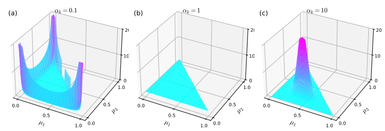
Figure 2.5 (reproduced). The Dirichlet density on the simplex of three variables for \(\alpha_k=0.1\) (mass in the corners), \(\alpha_k=1\) (uniform) and \(\alpha_k=10\) (a single peak at the centre). Book: Figure 2.5, p. 78 (the simplex itself is Figure 2.4, p. 77). Code: ch02_probability_distributions.py, fig2_5. Download: PDF · SVG
▶ DemoDirichlet on the simplex (Figure 2.5)Vary \(\alpha_1,\alpha_2,\alpha_3\) and add counts: the density concentrates where the observed frequencies lie.
Finally, the predictive distribution of the next state is \(p(x_k=1\given\mathcal{D})\)\({}=\E[\mu_k\given\mathcal{D}]\)\({}=\frac{\alpha_k+m_k}{\alpha_0+N}\), the \(K\)-state analogue of (2.20); with all \(\alpha_k=1\) it is the "add-one" (Laplace) smoothing used for word counts, which prevents the zero probabilities that maximum likelihood assigns to unseen states.
2.3 The Gaussian distribution
pp. 78–113 The Gaussian is the most widely used distribution for continuous variables. For one variable and for a \(D\)-dimensional vector,
Several reasons explain its role. It maximises the entropy for a given mean and variance (Result 2.13); the sum of many independent random variables tends to a Gaussian (the central limit theorem, below); it is closed under conditioning, marginalisation, linear maps and products (this section); and its parameters have an immediate meaning.
Filling the gap 2.1: why sums become Gaussian (Figure 2.6) p. 79
The book only shows (Figure 2.6) that the mean of \(N\) uniform variables looks more Gaussian as \(N\) grows. Here is the reason.
Derivation
Let \(x_1,x_2,\dots\) be i.i.d. with mean \(\mu\) and finite variance \(\sigma^2\), and \(S_N\)\({}=\frac1{\sqrt N}\sum_{n=1}^N\frac{x_n-\mu}{\sigma}\). The characteristic function \(\varphi(t)=\E[e^{it(x-\mu)/\sigma}]\) of one standardised term has the expansion \(\varphi(t)=1-\tfrac12t^2+o(t^2)\) as \(t\to0\) (mean zero, variance one). By independence, \(\E[e^{itS_N}]\)\({}=\varphi(t/\sqrt N)^N\)\({}=\big(1-\tfrac{t^2}{2N}+o(1/N)\big)^N\)\({}\to e^{-t^2/2}\), which is the characteristic function of \(\N(0,1)\). By Lévy's continuity theorem, \(S_N\) converges in distribution to \(\N(0,1)\); so the sample mean \(\bar x_N=\mu+\sigma S_N/\sqrt N\) is approximately \(\N(\mu,\sigma^2/N)\), whose variance shrinks as in Figure 2.6. The Gaussian is thus the only limit that survives averaging, because only for it is a sum of independent copies of the same shape again of that shape. ∎
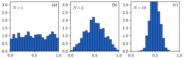
Figure 2.6 (reproduced). Histograms of the mean of \(N\) uniform numbers on \([0,1]\) for \(N=1,2,10\) (each from 10 000 draws): flat, triangular, then close to a bell curve. Book: Figure 2.6, p. 79. Code: ch02_probability_distributions.py, fig2_6. Download: PDF · SVG
Normalisation and moments
Result 2.7 (the Gaussian is normalised; its mean and covariance) (2.44)–(2.64); Exercises 2.17–2.23
Let \(\bm\Sigma\) be a real symmetric positive definite matrix with eigen-decomposition \(\bm\Sigma\mathbf{u}_i=\lambda_i\mathbf{u}_i\), \(\mathbf{u}_i^\T\mathbf{u}_j=\delta_{ij}\). Then \(\N(\mathbf{x}\given\bm\mu,\bm\Sigma)\) in (2.43) integrates to one, and
\[ \E[\mathbf{x}]=\bm\mu,\qquad \E[\mathbf{x}\mathbf{x}^\T]=\bm\mu\bm\mu^\T+\bm\Sigma,\qquad \cov[\mathbf{x}]=\bm\Sigma. \tag{2.59, 2.62, 2.64} \]
With \(\Delta^2\)\({}=(\mathbf{x}-\bm\mu)^\T\bm\Sigma^{-1}(\mathbf{x}-\bm\mu)\) the squared Mahalanobis distance (2.44), the surfaces of constant density are the ellipsoids \(\Delta^2=\) const, with axes along the \(\mathbf{u}_i\) and half-lengths \(\lambda_i^{1/2}\Delta\); the volume inside \(\Delta^2\le\Delta_0^2\) is \(V_D|\bm\Sigma|^{1/2}\Delta_0^D\) with \(V_D\) the volume of the unit ball (Exercise 2.23).
Proof
Step 1: eigen-expansion. With \(\mathbf{U}=(\mathbf{u}_1,\dots,\mathbf{u}_D)\) (orthogonal, \(\mathbf{U}^\T\mathbf{U}=\mathbf{I}\)) and \(\bm\Lambda_d=\diag(\lambda_i)\), \(\bm\Sigma\)\({}=\mathbf{U}\bm\Lambda_d\mathbf{U}^\T\)\({}=\sum_i\lambda_i\mathbf{u}_i\mathbf{u}_i^\T\) (2.48), \(\bm\Sigma^{-1}\)\({}=\sum_i\lambda_i^{-1}\mathbf{u}_i\mathbf{u}_i^\T\) (2.49) (multiply the two to check), so with \(y_i=\mathbf{u}_i^\T(\mathbf{x}-\bm\mu)\) (that is, \(\mathbf{y}=\mathbf{U}(\mathbf{x}-\bm\mu)\) in the book's notation (2.52)),
\[ \Delta^2=\sum_{i=1}^D\frac{y_i^2}{\lambda_i}.\tag{2.50} \]
Thus in the rotated, centred coordinates \(\mathbf{y}\) the contours are axis-aligned ellipsoids with semi-axes \(\lambda_i^{1/2}\Delta\), which proves the geometric statement; the \(\mathbf{u}_i\) give the directions and \(\lambda_i\) the variance along them. Also \(|\bm\Sigma|=\prod_i\lambda_i\) (2.55), as the determinant of an orthogonal matrix is \(\pm1\).
Step 2: normalisation. The map \(\mathbf{x}\mapsto\mathbf{y}\) is a rotation (possibly with a reflection) with Jacobian matrix \(\mathbf{U}\), \(|\det\mathbf{U}|=1\) (2.53, 2.54), so \(\d\mathbf{x}=\d\mathbf{y}\) and
\[ \int\!\N(\mathbf{x}\given\bm\mu,\bm\Sigma)\,\d\mathbf{x}=\prod_{j=1}^D\int\frac1{(2\pi\lambda_j)^{1/2}}\exp\Big\{-\frac{y_j^2}{2\lambda_j}\Big\}\d y_j=1,\]
because the exponent separates and \(\prod_j(2\pi\lambda_j)^{1/2}\)\({}=(2\pi)^{D/2}|\bm\Sigma|^{1/2}\) (2.55). Each one-dimensional factor is one: with \(I=\int e^{-y^2/2\lambda}\d y\), \(I^2\)\({}=\iint e^{-(y^2+z^2)/2\lambda}\d y\,\d z\)\({}=\int_0^{2\pi}\!\!\int_0^\infty e^{-r^2/2\lambda}r\,\d r\,\d\phi\)\({}=2\pi\lambda\) (polar coordinates), so \(I=(2\pi\lambda)^{1/2}\). Every \(\lambda_j>0\) is needed for integrability; if some \(\lambda_j\le0\) the integral diverges, which is why \(\bm\Sigma\) must be positive definite (Filling the gap 2.2).
Step 3: moments. Write \(\mathbf{x}=\bm\mu+\mathbf{z}\); the density of \(\mathbf{z}\) is even, so \(\E[\mathbf{z}]=\mathbf{0}\) (integral of an odd function over a symmetric domain) and \(\E[\mathbf{x}]=\bm\mu\). Then \(\E[\mathbf{x}\mathbf{x}^\T]\)\({}=\bm\mu\bm\mu^\T+\bm\mu\E[\mathbf{z}]^\T\)\({}+\E[\mathbf{z}]\bm\mu^\T\)\({}+\E[\mathbf{z}\mathbf{z}^\T]\), and with \(\mathbf{z}=\sum_jy_j\mathbf{u}_j\) (2.60), \(\E[\mathbf{z}\mathbf{z}^\T]\)\({}=\sum_{i,j}\mathbf{u}_i\mathbf{u}_j^\T\E[y_iy_j]\). The coordinates \(y_i\) are independent with \(y_i\sim\N(0,\lambda_i)\) (the density factorises in step 2), so \(\E[y_iy_j]=\delta_{ij}\lambda_i\) (the variance of \(\N(0,\lambda)\) is \(\lambda\): differentiate \(\int e^{-y^2/2\lambda}\d y=(2\pi\lambda)^{1/2}\) with respect to \(\lambda\), giving \(\int\frac{y^2}{2\lambda^2}e^{-y^2/2\lambda}\d y\)\({}=\frac12(2\pi)^{1/2}\lambda^{-1/2}\)). Hence \(\E[\mathbf{z}\mathbf{z}^\T]\)\({}=\sum_i\lambda_i\mathbf{u}_i\mathbf{u}_i^\T\)\({}=\bm\Sigma\) (2.61), which gives (2.62); and \(\cov[\mathbf{x}]\)\({}=\E[(\mathbf{x}-\bm\mu)(\mathbf{x}-\bm\mu)^\T]\)\({}=\E[\mathbf{z}\mathbf{z}^\T]\)\({}=\bm\Sigma\).
Step 4: volume. In \(\mathbf{y}\) coordinates the region is \(\sum_iy_i^2/\lambda_i\le\Delta_0^2\); put \(w_i=y_i/\lambda_i^{1/2}\), with Jacobian \(\prod_i\lambda_i^{1/2}=|\bm\Sigma|^{1/2}\). The region becomes the ball \(\|\mathbf{w}\|\le\Delta_0\) of volume \(V_D\Delta_0^D\), giving \(V_D|\bm\Sigma|^{1/2}\Delta_0^D\). ∎
Since \(\Delta^2=\sum_iy_i^2/\lambda_i\) is a sum of \(D\) squares of independent standard normals \(y_i/\lambda_i^{1/2}\), \(\Delta^2\) follows a chi-squared distribution with \(D\) degrees of freedom (mean \(D\)); this is why, for \(D=2\), the contour \(\Delta^2=5.99\) encloses 95% of the probability.
Filling the gap 2.2: the linear algebra behind the Gaussian pp. 80–84; Exercises 2.17–2.22
The book states four facts without proof: the precision matrix may be taken symmetric, the eigenvalues of a symmetric matrix are real with orthonormal eigenvectors, positive definiteness is equivalent to positive eigenvalues, and the parameter count is \(D(D+1)/2+D\). Proofs:
Derivation
Symmetry is no restriction (Exercise 2.17). Write any real matrix \(\mathbf{M}=\bm\Sigma^{-1}\) as \(\mathbf{M}=\mathbf{M}^{\rm S}+\mathbf{M}^{\rm A}\) with \(\mathbf{M}^{\rm S}\)\({}=\tfrac12(\mathbf{M}+\mathbf{M}^\T)\), \(\mathbf{M}^{\rm A}\)\({}=\tfrac12(\mathbf{M}-\mathbf{M}^\T)\). For any vector \(\mathbf{v}\), \(\mathbf{v}^\T\mathbf{M}^{\rm A}\mathbf{v}\) is a scalar equal to its own transpose \(\mathbf{v}^\T(\mathbf{M}^{\rm A})^\T\mathbf{v}\)\({}=-\mathbf{v}^\T\mathbf{M}^{\rm A}\mathbf{v}\), so it is zero. The exponent \(-\frac12(\mathbf{x}-\bm\mu)^\T\mathbf{M}(\mathbf{x}-\bm\mu)\) therefore does not see \(\mathbf{M}^{\rm A}\): only the symmetric part is identifiable, and we may assume \(\bm\Sigma^{-1}\) symmetric. The inverse of a symmetric invertible matrix is symmetric (Exercise 2.22): \((\bm\Sigma^{-1})^\T\)\({}=(\bm\Sigma^\T)^{-1}\)\({}=\bm\Sigma^{-1}\).
Real eigenvalues, orthonormal eigenvectors (Exercise 2.18). Let \(\bm\Sigma\mathbf{u}=\lambda\mathbf{u}\) with \(\mathbf{u}\ne\mathbf{0}\), possibly complex. Conjugating (\(\bm\Sigma\) is real): \(\bm\Sigma\bar{\mathbf{u}}\)\({}=\bar\lambda\bar{\mathbf{u}}\). Then \(\bar{\mathbf{u}}^\T\bm\Sigma\mathbf{u}\)\({}=\lambda\bar{\mathbf{u}}^\T\mathbf{u}\), while by symmetry \(\bar{\mathbf{u}}^\T\bm\Sigma\mathbf{u}\)\({}=(\bm\Sigma\bar{\mathbf{u}})^\T\mathbf{u}\)\({}=\bar\lambda\bar{\mathbf{u}}^\T\mathbf{u}\). Subtract: \((\lambda-\bar\lambda)\|\mathbf{u}\|^2=0\), so \(\lambda\) is real. If \(\bm\Sigma\mathbf{u}_i=\lambda_i\mathbf{u}_i\) and \(\bm\Sigma\mathbf{u}_j=\lambda_j\mathbf{u}_j\), then \(\mathbf{u}_i^\T\bm\Sigma\mathbf{u}_j\)\({}=\lambda_j\mathbf{u}_i^\T\mathbf{u}_j\)\({}=\lambda_i\mathbf{u}_i^\T\mathbf{u}_j\), so \((\lambda_i-\lambda_j)\mathbf{u}_i^\T\mathbf{u}_j\)\({}=0\): eigenvectors with distinct eigenvalues are orthogonal. Within an eigenspace of dimension greater than one (a repeated eigenvalue) any basis can be orthonormalised by Gram–Schmidt and stays inside the eigenspace. That there are \(D\) eigenvectors in total follows by induction: pick one real unit eigenvector \(\mathbf{u}_1\); \(\bm\Sigma\) maps its orthogonal complement into itself (\(\mathbf{v}\perp\mathbf{u}_1\)\({}\Rightarrow\mathbf{u}_1^\T\bm\Sigma\mathbf{v}\)\({}=\lambda_1\mathbf{u}_1^\T\mathbf{v}\)\({}=0\)), where it is again symmetric, and repeat. Zero eigenvalues cause no difficulty in any of this. Expansion (2.48): \(\mathbf{U}^\T\bm\Sigma\mathbf{U}=\bm\Lambda_d\) gives \(\bm\Sigma=\mathbf{U}\bm\Lambda_d\mathbf{U}^\T\), and \(\bm\Sigma^{-1}\)\({}=\mathbf{U}\bm\Lambda_d^{-1}\mathbf{U}^\T\) (2.49) (Exercise 2.19).
Positive definite \(\Leftrightarrow\) positive eigenvalues (Exercise 2.20). For any \(\mathbf{a}\), with \(a_i=\mathbf{u}_i^\T\mathbf{a}\) so that \(\mathbf{a}=\sum_ia_i\mathbf{u}_i\): \(\mathbf{a}^\T\bm\Sigma\mathbf{a}\)\({}=\sum_i\lambda_ia_i^2\). If all \(\lambda_i>0\) this is positive whenever \(\mathbf{a}\ne\mathbf{0}\) (some \(a_i\ne0\)). Conversely, taking \(\mathbf{a}=\mathbf{u}_i\) gives \(\lambda_i>0\).
Counting parameters (Exercise 2.21). A symmetric \(D\times D\) matrix is fixed by its diagonal (\(D\) entries) and strict upper triangle (\(D(D-1)/2\) entries): \(D(D+1)/2\) in all. With \(\bm\mu\), the Gaussian has \(D(D+3)/2\) free parameters: quadratic growth in \(D\). A diagonal covariance (Figure 2.8b) has \(D\) parameters and an isotropic one \(\sigma^2\mathbf{I}\) only one, at the price of axis-aligned or spherical contours. ∎
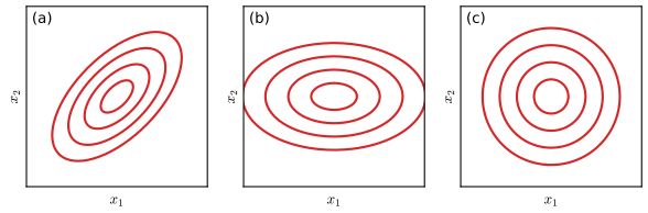
Figure 2.8 (reproduced). Contours of constant density of a two-dimensional Gaussian with (a) a general covariance matrix (ellipses tilted along the eigenvectors), (b) a diagonal covariance (axis-aligned ellipses), (c) an isotropic covariance \(\sigma^2\mathbf{I}\) (circles). Book: Figure 2.8, p. 84. Code: ch02_probability_distributions.py, fig2_8. Download: PDF · SVG
Limitations. A Gaussian has \(O(D^2)\) parameters, which becomes costly (inverting \(\bm\Sigma\) is \(O(D^3)\)) and can be reduced only by restricting the covariance, and it is unimodal and so cannot describe multimodal data. Both are addressed by latent variables: discrete ones give mixtures (Section 2.3.9, Chapter 9), continuous ones give factor analysis and probabilistic PCA (Chapter 12).
2.3.1 Conditional Gaussian distributions
pp. 85–88 Partition \(\mathbf{x}\sim\N(\bm\mu,\bm\Sigma)\) into \(\mathbf{x}_a\) (first \(M\) components) and \(\mathbf{x}_b\), with the corresponding blocks
with \(\bm\Sigma_{ba}=\bm\Sigma_{ab}^\T\), \(\bm\Lambda_{ba}=\bm\Lambda_{ab}^\T\). The blocks of \(\bm\Lambda\) are not the inverses of the blocks of \(\bm\Sigma\); the next result gives the relation.
Result 2.8 (partitioned matrix inverse) (2.76), (2.77), (2.78); Exercise 2.24
If \(\mathbf{D}\) is invertible and \(\mathbf{M}\)\({}=(\mathbf{A}-\mathbf{B}\mathbf{D}^{-1}\mathbf{C})^{-1}\) (the inverse of the Schur complement of \(\mathbf{D}\)) exists, then
\[ \begin{pmatrix}\mathbf{A}&\mathbf{B}\\\mathbf{C}&\mathbf{D}\end{pmatrix}^{-1}=\begin{pmatrix}\mathbf{M}&-\mathbf{M}\mathbf{B}\mathbf{D}^{-1}\\-\mathbf{D}^{-1}\mathbf{C}\mathbf{M}&\mathbf{D}^{-1}+\mathbf{D}^{-1}\mathbf{C}\mathbf{M}\mathbf{B}\mathbf{D}^{-1}\end{pmatrix}.\tag{2.76} \]
Consequently, for the covariance and precision blocks above,
\[ \bm\Lambda_{aa}=(\bm\Sigma_{aa}-\bm\Sigma_{ab}\bm\Sigma_{bb}^{-1}\bm\Sigma_{ba})^{-1},\qquad\bm\Lambda_{ab}=-(\bm\Sigma_{aa}-\bm\Sigma_{ab}\bm\Sigma_{bb}^{-1}\bm\Sigma_{ba})^{-1}\bm\Sigma_{ab}\bm\Sigma_{bb}^{-1}. \tag{2.78} \]
Proof
Multiply the claimed inverse on the left by \(\begin{pmatrix}\mathbf{A}&\mathbf{B}\\\mathbf{C}&\mathbf{D}\end{pmatrix}\) and check the four blocks. Top left: \(\mathbf{A}\mathbf{M}\)\({}-\mathbf{B}\mathbf{D}^{-1}\mathbf{C}\mathbf{M}\)\({}=(\mathbf{A}-\mathbf{B}\mathbf{D}^{-1}\mathbf{C})\mathbf{M}\)\({}=\mathbf{I}\). Top right: \(-\mathbf{A}\mathbf{M}\mathbf{B}\mathbf{D}^{-1}\)\({}+\mathbf{B}\mathbf{D}^{-1}\)\({}+\mathbf{B}\mathbf{D}^{-1}\mathbf{C}\mathbf{M}\mathbf{B}\mathbf{D}^{-1}\)\({}=-(\mathbf{A}-\mathbf{B}\mathbf{D}^{-1}\mathbf{C})\mathbf{M}\mathbf{B}\mathbf{D}^{-1}\)\({}+\mathbf{B}\mathbf{D}^{-1}\)\({}=\mathbf{0}\). Bottom left: \(\mathbf{C}\mathbf{M}\)\({}-\mathbf{D}\mathbf{D}^{-1}\mathbf{C}\mathbf{M}\)\({}=\mathbf{0}\). Bottom right: \(-\mathbf{C}\mathbf{M}\mathbf{B}\mathbf{D}^{-1}\)\({}+\mathbf{I}\)\({}+\mathbf{C}\mathbf{M}\mathbf{B}\mathbf{D}^{-1}\)\({}=\mathbf{I}\). A one-sided inverse of a square matrix is the inverse. Applying (2.76) to \(\bm\Sigma\) (with \(\mathbf{A}=\bm\Sigma_{aa}\), etc.) reads off the blocks of \(\bm\Lambda=\bm\Sigma^{-1}\). ∎
The same identity, rearranged, is the Woodbury formula (toolkit; Exercise 2.26 is proved in the solutions below).
Result 2.9 (conditional Gaussian) (2.70)–(2.82), (2.96), (2.97)
If \(\mathbf{x}\sim\N(\bm\mu,\bm\Sigma)\), then \(p(\mathbf{x}_a\given\mathbf{x}_b)\) is Gaussian with
\[ \bm\Sigma_{a|b}=\bm\Lambda_{aa}^{-1},\qquad\bm\mu_{a|b}=\bm\mu_a-\bm\Lambda_{aa}^{-1}\bm\Lambda_{ab}(\mathbf{x}_b-\bm\mu_b)\tag{2.73, 2.75} \]
or, in terms of the covariance blocks,
\[ \bm\mu_{a|b}=\bm\mu_a+\bm\Sigma_{ab}\bm\Sigma_{bb}^{-1}(\mathbf{x}_b-\bm\mu_b),\qquad\bm\Sigma_{a|b}=\bm\Sigma_{aa}-\bm\Sigma_{ab}\bm\Sigma_{bb}^{-1}\bm\Sigma_{ba}.\tag{2.81, 2.82} \]
The conditional mean is linear in \(\mathbf{x}_b\); the conditional covariance does not depend on \(\mathbf{x}_b\).
Proof
Fix \(\mathbf{x}_b\). As a function of \(\mathbf{x}_a\), \(p(\mathbf{x}_a\given\mathbf{x}_b)\)\({}\propto p(\mathbf{x}_a,\mathbf{x}_b)\), so only the terms of the exponent that contain \(\mathbf{x}_a\) matter. Expanding the quadratic form in the blocks of \(\bm\Lambda\),
\[ -\tfrac12(\mathbf{x}-\bm\mu)^\T\bm\Lambda(\mathbf{x}-\bm\mu)=-\tfrac12(\mathbf{x}_a-\bm\mu_a)^\T\bm\Lambda_{aa}(\mathbf{x}_a-\bm\mu_a)-\tfrac12(\mathbf{x}_a-\bm\mu_a)^\T\bm\Lambda_{ab}(\mathbf{x}_b-\bm\mu_b)-\tfrac12(\mathbf{x}_b-\bm\mu_b)^\T\bm\Lambda_{ba}(\mathbf{x}_a-\bm\mu_a)-\tfrac12(\mathbf{x}_b-\bm\mu_b)^\T\bm\Lambda_{bb}(\mathbf{x}_b-\bm\mu_b).\tag{2.70} \]
The two cross terms are equal (transpose of a scalar and \(\bm\Lambda_{ba}=\bm\Lambda_{ab}^\T\)). Keeping what depends on \(\mathbf{x}_a\):
\[ -\tfrac12\mathbf{x}_a^\T\bm\Lambda_{aa}\mathbf{x}_a+\mathbf{x}_a^\T\{\bm\Lambda_{aa}\bm\mu_a-\bm\Lambda_{ab}(\mathbf{x}_b-\bm\mu_b)\}+\mathrm{const}.\tag{2.74} \]
A Gaussian in \(\mathbf{x}_a\) with mean \(\mathbf{m}\) and covariance \(\mathbf{S}\) has exponent \(-\frac12\mathbf{x}_a^\T\mathbf{S}^{-1}\mathbf{x}_a\)\({}+\mathbf{x}_a^\T\mathbf{S}^{-1}\mathbf{m}+\) const (completing the square). Matching, \(\mathbf{S}=\bm\Lambda_{aa}^{-1}\) and \(\mathbf{S}^{-1}\mathbf{m}\)\({}=\bm\Lambda_{aa}\bm\mu_a\)\({}-\bm\Lambda_{ab}(\mathbf{x}_b-\bm\mu_b)\), i.e. \(\mathbf{m}\)\({}=\bm\mu_a\)\({}-\bm\Lambda_{aa}^{-1}\bm\Lambda_{ab}(\mathbf{x}_b-\bm\mu_b)\). The form in terms of \(\bm\Sigma\) follows by inserting (2.78): \(\bm\Lambda_{aa}^{-1}\)\({}=\bm\Sigma_{aa}\)\({}-\bm\Sigma_{ab}\bm\Sigma_{bb}^{-1}\bm\Sigma_{ba}\) and \(-\bm\Lambda_{aa}^{-1}\bm\Lambda_{ab}\)\({}=\bm\Sigma_{ab}\bm\Sigma_{bb}^{-1}\). ∎
Everything above is also derived in the toolkit (Gaussian facts) and toolkit (linear-Gaussian model). Note the economy of working with the precision: the conditional precision is just a sub-block of \(\bm\Lambda\) (no inversion), whereas the conditional covariance needs the Schur complement of \(\bm\Sigma\).
Three groups (Exercise 2.25). If \(\mathbf{x}\)\({}=(\mathbf{x}_a,\mathbf{x}_b,\mathbf{x}_c)\) and \(\mathbf{x}_c\) is to be integrated out, the marginal of \((\mathbf{x}_a,\mathbf{x}_b)\) is Gaussian with the corresponding sub-blocks of \(\bm\mu\) and \(\bm\Sigma\) (next section), so \(p(\mathbf{x}_a\given\mathbf{x}_b)\) is given by (2.81) and (2.82) using only \(\bm\Sigma_{aa},\bm\Sigma_{ab},\bm\Sigma_{bb}\): the covariance blocks involving \(\mathbf{x}_c\) are simply dropped.
2.3.2 Marginal Gaussian distributions
pp. 88–90 The marginal \(p(\mathbf{x}_a)\)\({}=\int p(\mathbf{x}_a,\mathbf{x}_b)\,\d\mathbf{x}_b\) is again Gaussian.
Result 2.10 (marginal Gaussian) (2.83)–(2.98)
\(p(\mathbf{x}_a)\)\({}=\N(\mathbf{x}_a\given\bm\mu_a,\bm\Sigma_{aa})\), i.e. \(\E[\mathbf{x}_a]=\bm\mu_a\) and \(\cov[\mathbf{x}_a]=\bm\Sigma_{aa}\) (2.92, 2.93). The marginal is read off the covariance blocks; the conditional is read off the precision blocks.
Proof
Use the centred variables \(\mathbf{y}_a=\mathbf{x}_a-\bm\mu_a\), \(\mathbf{y}_b=\mathbf{x}_b-\bm\mu_b\). The terms of the exponent (2.70) that contain \(\mathbf{y}_b\) are \(-\tfrac12\mathbf{y}_b^\T\bm\Lambda_{bb}\mathbf{y}_b\)\({}-\mathbf{y}_b^\T\bm\Lambda_{ba}\mathbf{y}_a\). Complete the square in \(\mathbf{y}_b\):
\[ -\tfrac12\mathbf{y}_b^\T\bm\Lambda_{bb}\mathbf{y}_b-\mathbf{y}_b^\T\bm\Lambda_{ba}\mathbf{y}_a=-\tfrac12(\mathbf{y}_b+\bm\Lambda_{bb}^{-1}\bm\Lambda_{ba}\mathbf{y}_a)^\T\bm\Lambda_{bb}(\mathbf{y}_b+\bm\Lambda_{bb}^{-1}\bm\Lambda_{ba}\mathbf{y}_a)+\tfrac12\mathbf{y}_a^\T\bm\Lambda_{ab}\bm\Lambda_{bb}^{-1}\bm\Lambda_{ba}\mathbf{y}_a. \]
(The book writes this with \(\mathbf{m}\)\({}=\bm\Lambda_{bb}\bm\mu_b\)\({}-\bm\Lambda_{ba}(\mathbf{x}_a-\bm\mu_a)\), (2.84, 2.85); the centred version is the same up to a shift of \(\mathbf{x}_b\).) The first term integrates over \(\mathbf{y}_b\) to the constant \((2\pi)^{M_b/2}|\bm\Lambda_{bb}|^{-1/2}\) which does not depend on \(\mathbf{x}_a\) (2.86). What is left of the exponent is
\[ -\tfrac12\mathbf{y}_a^\T\big(\bm\Lambda_{aa}-\bm\Lambda_{ab}\bm\Lambda_{bb}^{-1}\bm\Lambda_{ba}\big)\mathbf{y}_a. \]
By (2.76) applied to \(\bm\Lambda\) (its inverse is \(\bm\Sigma\)), the top-left block of \(\bm\Lambda^{-1}\) is \((\bm\Lambda_{aa}-\bm\Lambda_{ab}\bm\Lambda_{bb}^{-1}\bm\Lambda_{ba})^{-1}\), and equals \(\bm\Sigma_{aa}\) (2.91). So \(p(\mathbf{x}_a)\)\({}\propto\exp\{-\frac12(\mathbf{x}_a-\bm\mu_a)^\T\bm\Sigma_{aa}^{-1}(\mathbf{x}_a-\bm\mu_a)\}\), a Gaussian with the stated mean and covariance. ∎
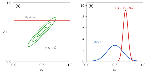
Figure 2.9 (reproduced). Left: contours of a bivariate Gaussian \(p(x_a,x_b)\) and the line \(x_b=0.7\). Right: the marginal \(p(x_a)\) (blue) and the conditional \(p(x_a\given x_b=0.7)\) (red): conditioning on a correlated variable shifts the mean and reduces the variance, by exactly the Schur complement. In our reconstruction (correlation \(\rho=0.95\); the book gives no numbers) the conditional mean is 0.690 with standard deviation 0.0437, against a marginal standard deviation of 0.140. Book: Figure 2.9, p. 90. Code: ch02_probability_distributions.py, fig2_9. Download: PDF · SVG
Two corollaries are used all the time. A sub-vector of a Gaussian vector is Gaussian with the matching sub-blocks of the mean and covariance, so uncorrelated components of a jointly Gaussian vector are independent (the covariance is block diagonal, so the density factorises). A Gaussian conditional, however, does not imply a Gaussian joint: jointly Gaussian is the strong assumption.
2.3.3 Bayes' theorem for Gaussian variables
pp. 90–93 Often one has a Gaussian marginal \(p(\mathbf{x})\) and a Gaussian conditional \(p(\mathbf{y}\given\mathbf{x})\) whose mean is linear in \(\mathbf{x}\), and wants \(p(\mathbf{y})\) and \(p(\mathbf{x}\given\mathbf{y})\) (a linear-Gaussian model; the probabilistic PCA and Kalman filter of Chapters 12 and 13 are built on it):
Result 2.11 (marginal and posterior for a linear-Gaussian model) (2.101)–(2.117); Exercises 2.27–2.33
The joint distribution of \(\mathbf{z}=(\mathbf{x},\mathbf{y})\) is Gaussian with
\[ \cov[\mathbf{z}]=\mathbf{R}^{-1}=\begin{pmatrix}\bm\Lambda^{-1}&\bm\Lambda^{-1}\mathbf{A}^\T\\\mathbf{A}\bm\Lambda^{-1}&\mathbf{L}^{-1}+\mathbf{A}\bm\Lambda^{-1}\mathbf{A}^\T\end{pmatrix},\qquad \E[\mathbf{z}]=\begin{pmatrix}\bm\mu\\\mathbf{A}\bm\mu+\mathbf{b}\end{pmatrix}.\tag{2.105, 2.108} \]
Hence the marginal and the posterior are
\[ p(\mathbf{y})=\N(\mathbf{y}\given\mathbf{A}\bm\mu+\mathbf{b},\ \mathbf{L}^{-1}+\mathbf{A}\bm\Lambda^{-1}\mathbf{A}^\T),\tag{2.115} \]
\[ p(\mathbf{x}\given\mathbf{y})=\N(\mathbf{x}\given\bm\Sigma\{\mathbf{A}^\T\mathbf{L}(\mathbf{y}-\mathbf{b})+\bm\Lambda\bm\mu\},\bm\Sigma),\qquad\bm\Sigma=(\bm\Lambda+\mathbf{A}^\T\mathbf{L}\mathbf{A})^{-1}.\tag{2.116, 2.117} \]
Proof
The joint is Gaussian. Its log is \(\ln p(\mathbf{x})\)\({}+\ln p(\mathbf{y}\given\mathbf{x})\)\({}=-\tfrac12(\mathbf{x}-\bm\mu)^\T\bm\Lambda(\mathbf{x}-\bm\mu)\)\({}-\tfrac12(\mathbf{y}-\mathbf{A}\mathbf{x}-\mathbf{b})^\T\mathbf{L}(\mathbf{y}-\mathbf{A}\mathbf{x}-\mathbf{b})\)\({}+\mathrm{const}\) (2.102), a quadratic in \(\mathbf{z}\), hence Gaussian. Precision. The terms of second order in \(\mathbf{z}\) are \[-\tfrac12[\mathbf{x}^\T(\bm\Lambda+\mathbf{A}^\T\mathbf{L}\mathbf{A})\mathbf{x}+\mathbf{y}^\T\mathbf{L}\mathbf{y}-\mathbf{y}^\T\mathbf{L}\mathbf{A}\mathbf{x}-\mathbf{x}^\T\mathbf{A}^\T\mathbf{L}\mathbf{y}]\]\({}=-\tfrac12\mathbf{z}^\T\mathbf{R}\mathbf{z}\) with
\[ \mathbf{R}=\begin{pmatrix}\bm\Lambda+\mathbf{A}^\T\mathbf{L}\mathbf{A}&-\mathbf{A}^\T\mathbf{L}\\-\mathbf{L}\mathbf{A}&\mathbf{L}\end{pmatrix}.\tag{2.104} \]
Covariance. Invert with (2.76) using \(\mathbf{D}=\mathbf{L}\): \(\mathbf{M}\)\({}=(\bm\Lambda+\mathbf{A}^\T\mathbf{L}\mathbf{A}-\mathbf{A}^\T\mathbf{L}\mathbf{L}^{-1}\mathbf{L}\mathbf{A})^{-1}\)\({}=\bm\Lambda^{-1}\), the top-right block is \(-\bm\Lambda^{-1}(-\mathbf{A}^\T\mathbf{L})\mathbf{L}^{-1}\)\({}=\bm\Lambda^{-1}\mathbf{A}^\T\), the bottom-left its transpose, and the bottom-right \(\mathbf{L}^{-1}\)\({}+\mathbf{L}^{-1}(-\mathbf{L}\mathbf{A})\bm\Lambda^{-1}(-\mathbf{A}^\T\mathbf{L})\mathbf{L}^{-1}\)\({}=\mathbf{L}^{-1}\)\({}+\mathbf{A}\bm\Lambda^{-1}\mathbf{A}^\T\) (Exercise 2.29). Mean. The terms linear in \(\mathbf{z}\) are \(\mathbf{x}^\T\bm\Lambda\bm\mu\)\({}-\mathbf{x}^\T\mathbf{A}^\T\mathbf{L}\mathbf{b}\)\({}+\mathbf{y}^\T\mathbf{L}\mathbf{b}\)\({}=\mathbf{z}^\T\binom{\bm\Lambda\bm\mu-\mathbf{A}^\T\mathbf{L}\mathbf{b}}{\mathbf{L}\mathbf{b}}\) (2.106); for a Gaussian with exponent \(-\frac12\mathbf{z}^\T\mathbf{R}\mathbf{z}\)\({}+\mathbf{z}^\T\mathbf{h}\) the mean is \(\mathbf{R}^{-1}\mathbf{h}\) (2.107). Multiplying out:
\[ \E[\mathbf{x}]=\bm\Lambda^{-1}(\bm\Lambda\bm\mu-\mathbf{A}^\T\mathbf{L}\mathbf{b})+\bm\Lambda^{-1}\mathbf{A}^\T\mathbf{L}\mathbf{b}=\bm\mu,\]
\[ \E[\mathbf{y}]=\mathbf{A}\bm\Lambda^{-1}(\bm\Lambda\bm\mu-\mathbf{A}^\T\mathbf{L}\mathbf{b})+(\mathbf{L}^{-1}+\mathbf{A}\bm\Lambda^{-1}\mathbf{A}^\T)\mathbf{L}\mathbf{b}=\mathbf{A}\bm\mu+\mathbf{b}\]
(Exercise 2.30). Marginal. By Result 2.10 the marginal of \(\mathbf{y}\) has the \(\mathbf{y}\) blocks of the mean and covariance: (2.115), i.e. (2.109, 2.110). Posterior. By Result 2.9 applied to the precision \(\mathbf{R}\) with \(\mathbf{x}\) in the role of \(\mathbf{x}_a\): \(\bm\Sigma_{x|y}\)\({}=\mathbf{R}_{xx}^{-1}\)\({}=(\bm\Lambda+\mathbf{A}^\T\mathbf{L}\mathbf{A})^{-1}\)\({}=\bm\Sigma\) and
\[ \bm\mu_{x|y}=\bm\mu-\mathbf{R}_{xx}^{-1}\mathbf{R}_{xy}(\mathbf{y}-\mathbf{A}\bm\mu-\mathbf{b})=\bm\mu+\bm\Sigma\mathbf{A}^\T\mathbf{L}(\mathbf{y}-\mathbf{A}\bm\mu-\mathbf{b}). \]
Since \(\bm\Sigma(\bm\Lambda+\mathbf{A}^\T\mathbf{L}\mathbf{A})\)\({}=\mathbf{I}\), \(\bm\mu\)\({}=\bm\Sigma(\bm\Lambda\bm\mu+\mathbf{A}^\T\mathbf{L}\mathbf{A}\bm\mu)\), and the mean becomes \(\bm\Sigma\{\bm\Lambda\bm\mu\)\({}+\mathbf{A}^\T\mathbf{L}(\mathbf{y}-\mathbf{b})\}\), as in (2.116). Erratum. The book's (2.111) misplaces the parenthesis; the form (2.116) is the correct one. ∎
This is the engine of Bayesian linear regression (Chapter 3), the Kalman filter (Section 13.3.1) and probabilistic PCA (Section 12.2). Reading it as inference: \(\mathbf{x}\) is a latent cause with prior precision \(\bm\Lambda\), \(\mathbf{y}\) an observation with noise precision \(\mathbf{L}\); the posterior precision \(\bm\Lambda+\mathbf{A}^\T\mathbf{L}\mathbf{A}\) is prior precision plus data precision, and the posterior mean is a precision-weighted compromise.
Filling the gap 2.3: the same results by completing the square directly (Exercises 2.32 and 2.33) p. 133
As an independent check, derive \(p(\mathbf{y})\) and \(p(\mathbf{x}\given\mathbf{y})\) without the joint covariance, using only completing the square and the Woodbury identity.
Derivation
Put \(\mathbf{S}\)\({}=\bm\Lambda+\mathbf{A}^\T\mathbf{L}\mathbf{A}\) and \(\mathbf{q}\)\({}=\bm\Lambda\bm\mu\)\({}+\mathbf{A}^\T\mathbf{L}(\mathbf{y}-\mathbf{b})\). Expanding the log joint (2.102) and keeping all terms, as a function of \(\mathbf{x}\),
\[ \ln p(\mathbf{x},\mathbf{y})=-\tfrac12\mathbf{x}^\T\mathbf{S}\mathbf{x}+\mathbf{x}^\T\mathbf{q}-\tfrac12(\mathbf{y}-\mathbf{b})^\T\mathbf{L}(\mathbf{y}-\mathbf{b})-\tfrac12\bm\mu^\T\bm\Lambda\bm\mu+\mathrm{const}. \]
Conditional. Completing the square in \(\mathbf{x}\): \(-\frac12(\mathbf{x}-\mathbf{S}^{-1}\mathbf{q})^\T\mathbf{S}(\mathbf{x}-\mathbf{S}^{-1}\mathbf{q})\)\({}+\frac12\mathbf{q}^\T\mathbf{S}^{-1}\mathbf{q}\), so \(p(\mathbf{x}\given\mathbf{y})\)\({}=\N(\mathbf{x}\given\mathbf{S}^{-1}\mathbf{q},\mathbf{S}^{-1})\), which is (2.116) (Exercise 2.33). Marginal. Integrating out \(\mathbf{x}\) leaves \(\frac12\mathbf{q}^\T\mathbf{S}^{-1}\mathbf{q}\) in the exponent. Its part that is quadratic in \(\mathbf{y}\) is \(\frac12\mathbf{y}^\T\mathbf{L}\mathbf{A}\mathbf{S}^{-1}\mathbf{A}^\T\mathbf{L}\mathbf{y}\), so the precision of \(\mathbf{y}\) is
\[ \mathbf{P}=\mathbf{L}-\mathbf{L}\mathbf{A}(\bm\Lambda+\mathbf{A}^\T\mathbf{L}\mathbf{A})^{-1}\mathbf{A}^\T\mathbf{L}=(\mathbf{L}^{-1}+\mathbf{A}\bm\Lambda^{-1}\mathbf{A}^\T)^{-1}, \]
the last equality being Woodbury's formula \((\mathbf{P}_0+\mathbf{B}\mathbf{C}\mathbf{D})^{-1}\)\({}=\mathbf{P}_0^{-1}\)\({}-\mathbf{P}_0^{-1}\mathbf{B}(\mathbf{C}^{-1}+\mathbf{D}\mathbf{P}_0^{-1}\mathbf{B})^{-1}\mathbf{D}\mathbf{P}_0^{-1}\) with \(\mathbf{P}_0=\mathbf{L}^{-1}\), \(\mathbf{B}=\mathbf{A}\), \(\mathbf{C}=\bm\Lambda^{-1}\), \(\mathbf{D}=\mathbf{A}^\T\). The terms linear in \(\mathbf{y}\) are \(\mathbf{y}^\T\mathbf{h}\), \(\mathbf{h}\)\({}=\mathbf{L}\mathbf{A}\mathbf{S}^{-1}(\bm\Lambda\bm\mu-\mathbf{A}^\T\mathbf{L}\mathbf{b})\)\({}+\mathbf{L}\mathbf{b}\) (one part from \(\frac12\mathbf{q}^\T\mathbf{S}^{-1}\mathbf{q}\), one from \(-\frac12(\mathbf{y}-\mathbf{b})^\T\mathbf{L}(\mathbf{y}-\mathbf{b})\)). The mean is \(\mathbf{P}^{-1}\mathbf{h}\); to check that it equals \(\mathbf{A}\bm\mu+\mathbf{b}\), verify \(\mathbf{P}(\mathbf{A}\bm\mu+\mathbf{b})\)\({}=\mathbf{h}\):
\[ \mathbf{P}(\mathbf{A}\bm\mu+\mathbf{b})-\mathbf{h}=\mathbf{L}\mathbf{A}\bm\mu-\mathbf{L}\mathbf{A}\mathbf{S}^{-1}\mathbf{A}^\T\mathbf{L}\mathbf{A}\bm\mu-\mathbf{L}\mathbf{A}\mathbf{S}^{-1}\bm\Lambda\bm\mu=\mathbf{L}\mathbf{A}\bm\mu-\mathbf{L}\mathbf{A}\mathbf{S}^{-1}\mathbf{S}\bm\mu=\mathbf{0}, \]
(the \(\mathbf{b}\) terms cancel in the same way). This reproduces (2.109) and (2.110), as Exercise 2.32 asks. ∎
Result 2.12 (sum of independent Gaussians) Exercises 2.27, 2.31
If \(\mathbf{x}\sim\N(\bm\mu_x,\bm\Sigma_x)\) and \(\mathbf{z}\sim\N(\bm\mu_z,\bm\Sigma_z)\) are independent, then \(\mathbf{y}\)\({}=\mathbf{x}+\mathbf{z}\)\({}\sim\N(\bm\mu_x+\bm\mu_z,\bm\Sigma_x+\bm\Sigma_z)\).
Proof
Given \(\mathbf{x}\), \(\mathbf{y}=\mathbf{x}+\mathbf{z}\) has the conditional \(\N(\mathbf{y}\given\mathbf{x}+\bm\mu_z,\bm\Sigma_z)\), which is (2.100) with \(\mathbf{A}=\mathbf{I}\), \(\mathbf{b}=\bm\mu_z\), \(\mathbf{L}^{-1}=\bm\Sigma_z\). With the marginal \(\N(\mathbf{x}\given\bm\mu_x,\bm\Sigma_x)\), (2.115) gives \(\N(\mathbf{y}\given\bm\mu_x+\bm\mu_z,\bm\Sigma_z+\bm\Sigma_x)\). (Without Gaussianity, means and covariances of independent summands still add, Exercise 2.27: \(\E[\mathbf{x}+\mathbf{z}]\)\({}=\E\mathbf{x}+\E\mathbf{z}\) and the cross term \(\E[(\mathbf{x}-\bm\mu_x)(\mathbf{z}-\bm\mu_z)^\T]\)\({}=\E[\mathbf{x}-\bm\mu_x]\E[\mathbf{z}-\bm\mu_z]^\T\)\({}=\mathbf{0}\) by independence.) ∎
Result 2.13 (entropy of the Gaussian; maximum entropy; KL divergence between Gaussians) Exercises 2.13–2.16, (2.279)–(2.284)
(a) \(\mathrm{H}[\N(\bm\mu,\bm\Sigma)]\)\({}=\tfrac12\ln|\bm\Sigma|+\tfrac D2(1+\ln2\pi)\) (2.283). (b) Among all densities with a given mean \(\bm\mu\) and covariance \(\bm\Sigma\), the Gaussian has the largest differential entropy. (c)
\[ \KL\big(\N(\bm\mu,\bm\Sigma)\,\|\,\N(\mathbf{m},\mathbf{L})\big)=\tfrac12\Big[\ln\frac{|\mathbf{L}|}{|\bm\Sigma|}-D+\Tr(\mathbf{L}^{-1}\bm\Sigma)+(\mathbf{m}-\bm\mu)^\T\mathbf{L}^{-1}(\mathbf{m}-\bm\mu)\Big]. \]
(d) If \(x_1\sim\N(\mu_1,\tau_1^{-1})\), \(x_2\sim\N(\mu_2,\tau_2^{-1})\) are independent, \(x=x_1+x_2\) has entropy \(\tfrac12\ln\{2\pi e(\tau_1^{-1}+\tau_2^{-1})\}\).
Proof
(a) \(-\ln\N(\mathbf{x}\given\bm\mu,\bm\Sigma)\)\({}=\tfrac D2\ln2\pi+\tfrac12\ln|\bm\Sigma|\)\({}+\tfrac12\Delta^2\) and \(\E[\Delta^2]\)\({}=\E[\Tr(\bm\Sigma^{-1}(\mathbf{x}-\bm\mu)(\mathbf{x}-\bm\mu)^\T)]\)\({}=\Tr(\bm\Sigma^{-1}\bm\Sigma)\)\({}=D\) (2.62). So \(\mathrm H\)\({}=\tfrac D2\ln2\pi+\tfrac12\ln|\bm\Sigma|\)\({}+\tfrac D2\).
(b) Variational derivation. Maximise \(-\int p\ln p\) subject to \(\int p=1\), \(\int p\,\mathbf{x}=\bm\mu\), \(\int p\,(\mathbf{x}-\bm\mu)(\mathbf{x}-\bm\mu)^\T\)\({}=\bm\Sigma\) (2.280–2.282), with multipliers \(\lambda_0\), \(\bm\lambda_1\) and a symmetric matrix \(\bm\Lambda_2\):
\[ \mathcal{F}[p]=-\!\int\!p\ln p\,\d\mathbf{x}+\lambda_0\Big(\int\!p-1\Big)+\bm\lambda_1^\T\Big(\int\!p\,\mathbf{x}-\bm\mu\Big)+\Tr\Big\{\bm\Lambda_2\Big(\int\!p(\mathbf{x}-\bm\mu)(\mathbf{x}-\bm\mu)^\T-\bm\Sigma\Big)\Big\}. \]
Setting the functional derivative (calculus of variations) to zero at each \(\mathbf{x}\): \(-\ln p(\mathbf{x})-1+\lambda_0\)\({}+\bm\lambda_1^\T\mathbf{x}\)\({}+(\mathbf{x}-\bm\mu)^\T\bm\Lambda_2(\mathbf{x}-\bm\mu)\)\({}=0\), so \(p(\mathbf{x})\)\({}=\exp\{\lambda_0-1+\bm\lambda_1^\T\mathbf{x}\)\({}+(\mathbf{x}-\bm\mu)^\T\bm\Lambda_2(\mathbf{x}-\bm\mu)\}\), the exponential of a quadratic. Normalisability needs \(\bm\Lambda_2\) negative definite, and completing the square shows the density is Gaussian; the constraints fix its mean \(\bm\mu\) and covariance \(\bm\Sigma\). This only finds a stationary point; here is why it is the maximum. Let \(q\) be any density with mean \(\bm\mu\) and covariance \(\bm\Sigma\) and \(g=\N(\bm\mu,\bm\Sigma)\). Since \(\ln g\) is a quadratic in \(\mathbf{x}\), \(\E_q[\ln g]\) depends on \(q\) only through its first two moments, so \(\E_q[\ln g]=\E_g[\ln g]=-\mathrm H[g]\). Then \(0\)\({}\le\KL(q\|g)\)\({}=-\mathrm H[q]-\E_q[\ln g]\)\({}=\mathrm H[g]-\mathrm H[q]\) (Gibbs' inequality, toolkit), with equality iff \(q=g\).
(c) \(\KL\)\({}=\E_p[\ln p]-\E_p[\ln q]\)\({}=-\mathrm H[p]+\tfrac D2\ln2\pi\)\({}+\tfrac12\ln|\mathbf{L}|\)\({}+\tfrac12\E_p[(\mathbf{x}-\mathbf{m})^\T\mathbf{L}^{-1}(\mathbf{x}-\mathbf{m})]\). Here \(\E_p[(\mathbf{x}-\mathbf{m})^\T\mathbf{L}^{-1}(\mathbf{x}-\mathbf{m})]\)\({}=\Tr(\mathbf{L}^{-1}\bm\Sigma)\)\({}+(\bm\mu-\mathbf{m})^\T\mathbf{L}^{-1}(\bm\mu-\mathbf{m})\) (write \(\mathbf{x}-\mathbf{m}\)\({}=(\mathbf{x}-\bm\mu)+(\bm\mu-\mathbf{m})\); the cross term has zero mean). Substituting (a) gives the formula. (Here \(\mathbf{L}\) is a covariance matrix, as in the exercise.)
(d) Given \(x_2\), \(x\sim\N(\mu_1+x_2,\tau_1^{-1})\). Then \(p(x)\)\({}=\int\N(x\given\mu_1+x_2,\tau_1^{-1})\N(x_2\given\mu_2,\tau_2^{-1})\d x_2\); the exponent in \(x_2\) is \(-\tfrac{\tau_1}2(x-\mu_1-x_2)^2\)\({}-\tfrac{\tau_2}2(x_2-\mu_2)^2\). Completing the square in \(x_2\) leaves \(-\tfrac12\frac{\tau_1\tau_2}{\tau_1+\tau_2}(x-\mu_1-\mu_2)^2\) (the standard convolution computation; or apply Result 2.12 in one dimension), so \(x\) is Gaussian with variance \(\tau_1^{-1}+\tau_2^{-1}\), and (a) in one dimension gives the entropy \(\tfrac12\ln\{2\pi e\,\mathrm{var}\}\). ∎
2.3.4 Maximum likelihood for the Gaussian
pp. 93–94 For i.i.d. data \(\mathbf{X}=(\mathbf{x}_1,\dots,\mathbf{x}_N)^\T\) from \(\N(\bm\mu,\bm\Sigma)\),
The data enter only through \(\sum_n\mathbf{x}_n\) and \(\sum_n\mathbf{x}_n\mathbf{x}_n^\T\), the sufficient statistics (2.119).
Result 2.14 (ML for the Gaussian; the covariance estimator is biased) (2.120)–(2.125); Exercises 2.34, 2.35
The maximisers are the sample mean and the sample covariance about it,
\[ \bm\mu_{\rm ML}=\frac1N\sum_{n=1}^N\mathbf{x}_n,\qquad \bm\Sigma_{\rm ML}=\frac1N\sum_{n=1}^N(\mathbf{x}_n-\bm\mu_{\rm ML})(\mathbf{x}_n-\bm\mu_{\rm ML})^\T.\tag{2.121, 2.122} \]
Under the true distribution, \(\E[\bm\mu_{\rm ML}]=\bm\mu\) and \(\E[\bm\Sigma_{\rm ML}]=\frac{N-1}N\bm\Sigma\) (2.123, 2.124), so the unbiased version is
\[ \widetilde{\bm\Sigma}=\frac1{N-1}\sum_{n=1}^N(\mathbf{x}_n-\bm\mu_{\rm ML})(\mathbf{x}_n-\bm\mu_{\rm ML})^\T.\tag{2.125} \]
Proof
Mean. The gradient with respect to \(\bm\mu\) is \(\sum_n\bm\Sigma^{-1}(\mathbf{x}_n-\bm\mu)\) (2.120) (toolkit: \(\nabla_{\bm\mu}\,\frac12(\mathbf{x}-\bm\mu)^\T\bm\Sigma^{-1}(\mathbf{x}-\bm\mu)\)\({}=-\bm\Sigma^{-1}(\mathbf{x}-\bm\mu)\) for symmetric \(\bm\Sigma\)); setting it to zero and multiplying by \(\bm\Sigma\) gives (2.121), whatever \(\bm\Sigma\) is.
Covariance (Exercise 2.34). Differentiate (2.118) with respect to \(\bm\Sigma\), ignoring symmetry, using \(\partial\ln|\bm\Sigma|/\partial\bm\Sigma\)\({}=\bm\Sigma^{-\T}\) and \(\partial\Tr(\bm\Sigma^{-1}\mathbf{A})/\partial\bm\Sigma\)\({}=-\bm\Sigma^{-\T}\mathbf{A}^\T\bm\Sigma^{-\T}\) (Appendix C (C.28), (C.21), (C.26) in the book, toolkit). Write \(\sum_n(\mathbf{x}_n-\bm\mu)^\T\bm\Sigma^{-1}(\mathbf{x}_n-\bm\mu)\)\({}=\Tr(\bm\Sigma^{-1}\mathbf{S}_\mu)\) with \(\mathbf{S}_\mu\)\({}=\sum_n(\mathbf{x}_n-\bm\mu)(\mathbf{x}_n-\bm\mu)^\T\). The gradient is
\[ -\frac N2\bm\Sigma^{-1}+\frac12\bm\Sigma^{-1}\mathbf{S}_\mu\bm\Sigma^{-1}=\mathbf{0}\ \Rightarrow\ \bm\Sigma=\frac1N\mathbf{S}_\mu, \]
(everything symmetric). Together with the mean this is (2.122) at \(\bm\mu=\bm\mu_{\rm ML}\). That it is a maximum over positive definite matrices: in terms of \(\bm\Lambda=\bm\Sigma^{-1}\) the log likelihood is \(\frac N2\ln|\bm\Lambda|\)\({}-\frac12\Tr(\bm\Lambda\mathbf{S}_\mu)+\)const, which is concave in \(\bm\Lambda\) (\(\ln|\cdot|\) is concave, the trace term is linear), so the stationary point is the global maximum (and maximum likelihood is invariant to the reparametrisation \(\bm\Sigma\leftrightarrow\bm\Lambda\)). It exists as a positive definite matrix when \(N>D\) and the data are not in a proper affine subspace.
Bias (Exercise 2.35). For independent samples with mean \(\bm\mu\) and covariance \(\bm\Sigma\): \(\E[\mathbf{x}_n\mathbf{x}_m^\T]\)\({}=\bm\mu\bm\mu^\T+I_{nm}\bm\Sigma\) (2.291) (for \(n\ne m\) the expectation factorises; for \(n=m\) use (2.62); this is the corrected form, the book's (2.291) lost a transpose). Hence \(\E[\bm\mu_{\rm ML}]=\bm\mu\) (2.123) and, using \(\bm\Sigma_{\rm ML}\)\({}=\frac1N\sum_n\mathbf{x}_n\mathbf{x}_n^\T\)\({}-\bm\mu_{\rm ML}\bm\mu_{\rm ML}^\T\),
\[ \E\Big[\frac1N\sum_n\mathbf{x}_n\mathbf{x}_n^\T\Big]=\bm\mu\bm\mu^\T+\bm\Sigma,\qquad \E[\bm\mu_{\rm ML}\bm\mu_{\rm ML}^\T]=\frac1{N^2}\sum_{n,m}(\bm\mu\bm\mu^\T+I_{nm}\bm\Sigma)=\bm\mu\bm\mu^\T+\frac1N\bm\Sigma. \]
Subtracting, \(\E[\bm\Sigma_{\rm ML}]=\frac{N-1}{N}\bm\Sigma\) (2.124). The bias arises because \(\bm\mu_{\rm ML}\) is fitted to the same points, so the residuals are too small; the factor \(N/(N-1)\) in (2.125) removes it. The bias vanishes as \(N\to\infty\), but matters for small \(N\) (for \(N=1\), \(\bm\Sigma_{\rm ML}=\mathbf{0}\)); it is the same effect as the underestimation of the variance that causes over-fitting in polynomial curve fitting (Section 1.2.5). ∎
2.3.5 Sequential estimation
pp. 94–97 Sequential (on-line) methods process one observation at a time and discard it, which is essential for large or streaming data sets. Separating the last term of (2.121),
The new estimate is the old one moved towards the new point, by a step that shrinks like \(1/N\) ("error signal" \(\mathbf{x}_N-\bm\mu^{(N-1)}\)). It is exact: check by multiplying (2.126) by \(N\). But this trick does not exist for every estimator, hence the general Robbins–Monro procedure.
Let \(z\) and \(\theta\) be correlated random variables with the regression function \(f(\theta)\)\({}=\E[z\given\theta]\)\({}=\int zp(z\given\theta)\d z\) (2.127), and suppose we want the root \(\theta^\star\) of \(f(\theta^\star)=0\) when we can only draw noisy samples of \(z\) (Figure 2.10). Assume \(\E[(z-f)^2\given\theta]<\infty\) (2.128) and, without loss of generality, \(f(\theta)>0\) for \(\theta>\theta^\star\), \(f(\theta)<0\) for \(\theta<\theta^\star\). The procedure is
Result 2.15 (Robbins–Monro: convergence in mean square) (2.127)–(2.132), Robbins and Monro (1951)
Suppose, in addition to (2.128), that for some constants \(c,K>0\): \((\theta-\theta^\star)f(\theta)\)\({}\ge c(\theta-\theta^\star)^2\) and \(\E[z^2\given\theta]\)\({}\le K\{1+(\theta-\theta^\star)^2\}\). If the steps obey (2.130)–(2.132), the iterates (2.129) satisfy \(\E[(\theta^{(N)}-\theta^\star)^2]\to0\), hence converge to \(\theta^\star\) in probability. (Robbins and Monro prove convergence under weaker conditions; the assumptions here make the argument short and show the role of each condition.)
Proof
Let \(d_N=\E[(\theta^{(N)}-\theta^\star)^2]\) and \(\delta=\theta^{(N-1)}-\theta^\star\). Squaring (2.129) and conditioning on \(\theta^{(N-1)}\) (the new sample \(z\) is drawn from \(p(z\given\theta^{(N-1)})\)):
\[ \E[(\theta^{(N)}-\theta^\star)^2\given\theta^{(N-1)}]=\delta^2-2a_{N-1}\delta f(\theta^{(N-1)})+a_{N-1}^2\E[z^2\given\theta^{(N-1)}]\le(1-2ca_{N-1}+Ka_{N-1}^2)\delta^2+Ka_{N-1}^2. \]
Taking expectations, \(d_N\le\beta_{N-1}d_{N-1}+Ka_{N-1}^2\) with \(\beta_N=1-2ca_N+Ka_N^2\). Since \(a_N\to0\) (2.130) there is \(N_0\) with \(0<\beta_N\le1-ca_N\) for \(N\ge N_0\). Lemma: if \(d_N\le\beta_{N-1}d_{N-1}+Ka_{N-1}^2\) with such \(\beta\), \(\sum a_N=\infty\) and \(\sum a_N^2<\infty\), then \(d_N\to0\). Unrolling from \(N_0\),
\[ d_N\le\Big(\prod_{k=N_0}^{N-1}\beta_k\Big)d_{N_0}+K\sum_{j=N_0}^{N-1}a_j^2\prod_{k=j+1}^{N-1}\beta_k . \]
The first term is at most \(e^{-c\sum_{k=N_0}^{N-1}a_k}d_{N_0}\to0\) because \(\sum a_k=\infty\) (2.131). In the sum, given \(\varepsilon>0\) choose \(J\) so that \(K\sum_{j>J}a_j^2<\varepsilon\) (possible because \(\sum a_j^2<\infty\), (2.132)); the terms with \(j>J\) contribute less than \(\varepsilon\) since every product is at most \(1\), while the finitely many terms with \(j\le J\) are multiplied by \(e^{-c\sum_{k>J}^{N-1}a_k}\to0\). So \(\limsup d_N\le\varepsilon\) for every \(\varepsilon\). ∎
The roles of the conditions: (2.130) lets the iterates settle, (2.131) lets them travel arbitrarily far, so a bad start is forgotten, and (2.132) makes the accumulated noise \(\sum a_N^2\,\mathrm{var}(z)\) finite. The choice \(a_N=1/(N+1)\) (or \(c/N\)) satisfies all three.
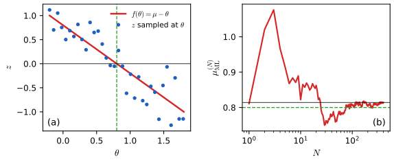
Figure 2.11 (our own computed run). For a Gaussian with known variance, the regression function of Figure 2.10, as a function of the current estimate \(\theta=\mu_{\rm ML}\), is the straight line \(f(\theta)=(\theta-\mu)/\sigma^2\) with slope \(1/\sigma^2\); noisy samples of \(z=-(x-\mu_{\rm ML})/\sigma^2\) scatter around it (a computed Robbins–Monro run, not the book's sketch) and its root is the true mean \(\mu\) (Erratum: the labels \(\mu\) and \(\mu_{\rm ML}\) are exchanged in the book's figure). Book: Figure 2.11, p. 97 (the schematic Figure 2.10 is on p. 95). Code: ch02_probability_distributions.py, fig2_11. Download: PDF · SVG
Filling the gap 2.4: Robbins–Monro applied to maximum likelihood (the Gaussian, and its variance and covariance) pp. 96–97, (2.133)–(2.137); Exercises 2.36, 2.37
At the ML solution the gradient of the log likelihood vanishes (2.133), and as \(N\to\infty\) the sample average tends to the expectation, so \(\theta_{\rm ML}\) is the root of the regression function \(f(\theta)\)\({}=\E_x[-\partial_\theta\ln p(x\given\theta)]\) (2.134). Taking \(z=-\partial_\theta\ln p(x\given\theta)\) in (2.129) gives the sequential algorithm
Why \(f\) has this form. Under the true parameter \(\theta_0\), the expected score vanishes, \(\E_{x}[\partial_\theta\ln p(x\given\theta)]_{\theta_0}\)\({}=\int\partial_\theta p\)\({}=\partial_\theta\int p\)\({}=0\), so \(\theta_0\) is a root of \(f\), and the Robbins–Monro iterate (2.135) converges to it when its conditions hold.
Mean of a Gaussian. For the mean \(\theta\) with known \(\sigma^2\), \(z\)\({}=-\partial_\theta\ln\N(x\given\theta,\sigma^2)\)\({}=-(x-\theta)/\sigma^2\) (2.136, with the minus signs of the errata). If \(x\) comes from \(\N(\mu,\sigma^2)\), \(f(\theta)\)\({}=\E[z\given\theta]\)\({}=(\theta-\mu)/\sigma^2\): a straight line with slope \(1/\sigma^2\) and root at the true mean (Figure 2.11), so the conditions of Result 2.15 hold with \(c=1/\sigma^2\). Equation (2.135) reads \(\theta^{(N)}\)\({}=\theta^{(N-1)}\)\({}+\frac{a_{N-1}}{\sigma^2}(x_N-\theta^{(N-1)})\), which is (2.126) when \(a_{N-1}=\sigma^2/N\); this choice satisfies (2.130)–(2.132), so (2.126) is a Robbins–Monro procedure.
Variance (Exercise 2.36). With \(\mu\) known, \(\sigma^2_{(N)}=\frac1N\sum_n(x_n-\mu)^2\) obeys \(\sigma^2_{(N)}\)\({}=\sigma^2_{(N-1)}+\frac1N\{(x_N-\mu)^2\)\({}-\sigma^2_{(N-1)}\}\) (separate the last term, as for (2.126)). Robbins–Monro with \(z\)\({}=-\partial_{\sigma^2}\ln\N(x\given\mu,\sigma^2)\)\({}=\frac1{2\sigma^2}-\frac{(x-\mu)^2}{2\sigma^4}\) gives
\[ \sigma^2_{(N)}=\sigma^2_{(N-1)}-a_{N-1}\Big[\frac1{2\sigma^2_{(N-1)}}-\frac{(x_N-\mu)^2}{2\sigma^4_{(N-1)}}\Big]=\sigma^2_{(N-1)}+\frac{a_{N-1}}{2\sigma^4_{(N-1)}}\big\{(x_N-\mu)^2-\sigma^2_{(N-1)}\big\}, \]
the same form, and it coincides with the exact sequential update when \(a_{N-1}=2\sigma^4_{(N-1)}/N\) (asymptotically \(2\sigma^4/N\), which satisfies the three conditions since \(\sigma^2_{(N)}\to\sigma^2\)). The regression function is \(f(\sigma^2)\)\({}=(\sigma^2-\sigma^2_{\rm true})/(2\sigma^4)\), increasing through its root.
Covariance (Exercise 2.37). With \(\bm\mu\) known, (2.122) gives \(\bm\Sigma^{(N)}\)\({}=\bm\Sigma^{(N-1)}\)\({}+\frac1N\{(\mathbf{x}_N-\bm\mu)(\mathbf{x}_N-\bm\mu)^\T\)\({}-\bm\Sigma^{(N-1)}\}\). In the Robbins–Monro form, \(\mathbf{Z}\)\({}=-\partial_{\bm\Sigma}\ln\N\)\({}=\frac12\bm\Sigma^{-1}\{\mathbf{I}\)\({}-(\mathbf{x}-\bm\mu)(\mathbf{x}-\bm\mu)^\T\bm\Sigma^{-1}\}\), so \(\bm\Sigma^{(N)}\)\({}=\bm\Sigma^{(N-1)}\)\[{}+\frac12\mathcal{A}_{N-1}[\bm\Sigma^{-1}\{(\mathbf{x}_N-\bm\mu)(\mathbf{x}_N-\bm\mu)^\T-\bm\Sigma^{(N-1)}\}\bm\Sigma^{-1}]\] with a matrix-valued gain; it matches the exact recursion when the gain operator is \(\mathcal{A}_{N-1}[\mathbf{M}]\)\({}=\frac2N\bm\Sigma^{(N-1)}\mathbf{M}\bm\Sigma^{(N-1)}\), i.e. a scalar step \(a_N\approx 2/N\) in the natural metric of covariances. When \(\bm\mu\) is also estimated, Welford's identity \(\sum_{n\le N}(\mathbf{x}_n-\bm\mu^{(N)})(\cdot)^\T\)\({}=\sum_{n\le N-1}(\mathbf{x}_n-\bm\mu^{(N-1)})(\cdot)^\T\)\({}+\frac{N-1}N(\mathbf{x}_N-\bm\mu^{(N-1)})(\cdot)^\T\) gives the exact update \(\bm\Sigma_{\rm ML}^{(N)}\)\({}=\bm\Sigma_{\rm ML}^{(N-1)}\)\({}+\frac1N\big\{\frac{N-1}N(\mathbf{x}_N-\bm\mu^{(N-1)})(\mathbf{x}_N-\bm\mu^{(N-1)})^\T\)\({}-\bm\Sigma_{\rm ML}^{(N-1)}\big\}\). ∎
2.3.6 Bayesian inference for the Gaussian
pp. 97–103 Maximum likelihood gives point estimates; a Bayesian treatment gives a posterior. Three cases: unknown mean with known variance, unknown variance with known mean, and both unknown. In each, a prior of the same form as the likelihood (as a function of the unknown) is conjugate.
Unknown mean, known variance
For \(N\) scalar observations \(\mathbf{x}=(x_1,\dots,x_N)^\T\) (the book's notation, erratum: lower-case \(x\) throughout this section), the likelihood as a function of \(\mu\) is
an exponential of a quadratic in \(\mu\), so a Gaussian prior \(p(\mu)=\N(\mu\given\mu_0,\sigma_0^2)\) (2.138) is conjugate.
Result 2.16 (posterior for the mean of a Gaussian with known variance) (2.139)–(2.144); Exercises 2.38–2.40
With prior \(\N(\mu\given\mu_0,\sigma_0^2)\), the posterior is \(p(\mu\given\mathbf{x})\)\({}=\N(\mu\given\mu_N,\sigma_N^2)\) with
\[ \mu_N=\frac{\sigma^2}{N\sigma_0^2+\sigma^2}\mu_0+\frac{N\sigma_0^2}{N\sigma_0^2+\sigma^2}\mu_{\rm ML},\qquad\frac1{\sigma_N^2}=\frac1{\sigma_0^2}+\frac N{\sigma^2},\qquad\mu_{\rm ML}=\frac1N\sum_nx_n. \tag{2.141--2.143} \]
Sequentially, the posterior after \(N-1\) points acts as the prior for the \(N\)-th, with \(\mu_N\)\({}=\dfrac{\sigma^2\mu_{N-1}+\sigma_{N-1}^2x_N}{\sigma^2+\sigma_{N-1}^2}\) and \(\sigma_N^{-2}=\sigma_{N-1}^{-2}+\sigma^{-2}\). For a \(D\)-dimensional vector with known \(\bm\Sigma\) and prior \(\N(\bm\mu\given\bm\mu_0,\bm\Sigma_0)\): \(\bm\Sigma_N^{-1}\)\({}=\bm\Sigma_0^{-1}+N\bm\Sigma^{-1}\) and \(\bm\mu_N\)\({}=\bm\Sigma_N(\bm\Sigma^{-1}N\bar{\mathbf{x}}+\bm\Sigma_0^{-1}\bm\mu_0)\).
Proof
\(p(\mu\given\mathbf{x})\)\({}\propto p(\mathbf{x}\given\mu)p(\mu)\) (2.139). Keep the exponent's \(\mu\)-dependence:
\[ -\frac1{2\sigma^2}\sum_n(x_n-\mu)^2-\frac1{2\sigma_0^2}(\mu-\mu_0)^2=-\frac12\Big(\frac N{\sigma^2}+\frac1{\sigma_0^2}\Big)\mu^2+\mu\Big(\frac{N\mu_{\rm ML}}{\sigma^2}+\frac{\mu_0}{\sigma_0^2}\Big)+\mathrm{const}, \]
using \(\sum_nx_n=N\mu_{\rm ML}\). Match to \(-\frac1{2\sigma_N^2}\mu^2+\mu\mu_N/\sigma_N^2\): \(\sigma_N^{-2}=\sigma_0^{-2}+N\sigma^{-2}\), and \(\mu_N\)\({}=\sigma_N^2(N\mu_{\rm ML}/\sigma^2+\mu_0/\sigma_0^2)\)\({}=\frac{\sigma^2\sigma_0^2}{\sigma^2+N\sigma_0^2}(\cdot)\), which is the weighted form in (2.141). Sequential form. Apply the one-observation case to the prior \(\N(\mu_{N-1},\sigma_{N-1}^2)\): precision \(\sigma_{N-1}^{-2}+\sigma^{-2}\), mean \(\sigma_N^2(\mu_{N-1}/\sigma_{N-1}^2+x_N/\sigma^2)\)\({}=(\sigma^2\mu_{N-1}+\sigma_{N-1}^2x_N)/(\sigma^2+\sigma_{N-1}^2)\); expanding \(\mu_{N-1},\sigma_{N-1}^2\) by (2.141) and (2.142) shows this equals the batch result (Exercise 2.39). Multivariate. The same steps with matrices (Exercise 2.40): the exponent is \(-\frac12\bm\mu^\T(\bm\Sigma_0^{-1}+N\bm\Sigma^{-1})\bm\mu\)\({}+\bm\mu^\T(\bm\Sigma_0^{-1}\bm\mu_0+\bm\Sigma^{-1}\textstyle\sum_n\mathbf{x}_n)\). ∎
Reading the result. Precisions add (information accumulates); the mean is a precision-weighted average of prior mean and ML estimate. For \(N=0\) the posterior is the prior; as \(N\to\infty\), \(\mu_N\to\mu_{\rm ML}\) and \(\sigma_N^2\to0\) like \(\sigma^2/N\) (the posterior concentrates). A broad prior \(\sigma_0^2\to\infty\) reduces the posterior mean to \(\mu_{\rm ML}\) and variance to \(\sigma^2/N\): the non-informative limit (Section 2.4.3). The posterior mean is a shrinkage estimator: it moves \(\mu_{\rm ML}\) toward \(\mu_0\) by an amount that decreases with \(N\).
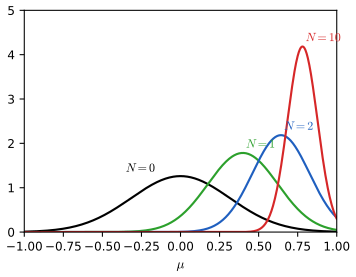
Figure 2.12 (reproduced). Bayesian inference for the mean of a Gaussian with known variance: the prior (\(N=0\)) and the posterior after \(N=1,2,10\) observations drawn from a Gaussian with mean \(0.8\) and variance \(0.1\), with a prior \(\N(0,0.1)\). The posterior narrows toward the true mean. The data are our reconstruction; settings are in the module docstring. Book: Figure 2.12, p. 99. Code: ch02_probability_distributions.py, fig2_12. Download: PDF · SVG
With the precision \(\lambda=1/\sigma^2\) as the unknown, the likelihood is proportional to \(\lambda^{N/2}\exp\{-\frac\lambda2\sum_n(x_n-\mu)^2\}\) (2.145): a power of \(\lambda\) times an exponential in \(\lambda\), the form of the gamma distribution
Result 2.17 (the gamma distribution; posterior for the precision) (2.146)–(2.151); Exercises 2.41, 2.42
(a) \(\Gam(\lambda\given a,b)\) is normalised, with the mean, variance and mode above. (b) With prior \(\Gam(\lambda\given a_0,b_0)\) and the Gaussian likelihood with known \(\mu\), the posterior is \(\Gam(\lambda\given a_N,b_N)\) with
\[ a_N=a_0+\frac N2,\qquad b_N=b_0+\frac12\sum_{n=1}^N(x_n-\mu)^2=b_0+\frac N2\sigma^2_{\rm ML}.\tag{2.150, 2.151} \]
Proof
(a) Substitute \(u=b\lambda\): \(\int_0^\infty\lambda^{a-1}e^{-b\lambda}\d\lambda\)\({}=b^{-a}\int_0^\infty u^{a-1}e^{-u}\d u\)\({}=b^{-a}\Gamma(a)\). Likewise \(\E[\lambda^k]\)\({}=\frac{b^a}{\Gamma(a)}\int\lambda^{a+k-1}e^{-b\lambda}\d\lambda\)\({}=\frac{\Gamma(a+k)}{\Gamma(a)b^k}\), so \(\E[\lambda]=a/b\), \(\E[\lambda^2]=a(a+1)/b^2\), \(\var[\lambda]=a/b^2\). The log density \((a-1)\ln\lambda-b\lambda\) has derivative \((a-1)/\lambda-b\), zero at \(\lambda=(a-1)/b\), a maximum for \(a>1\) (concave); for \(a\le1\) the density is largest at \(\lambda\to0\).
(b) Prior times likelihood: \(\lambda^{a_0-1}e^{-b_0\lambda}\cdot\lambda^{N/2}\exp\{-\frac\lambda2\sum_n(x_n-\mu)^2\}\)\[{}=\lambda^{a_0+N/2-1}\exp\{-\lambda(b_0+\frac12\sum_n(x_n-\mu)^2)\}\], a gamma density with the stated parameters. ∎
So the prior is equivalent to \(2a_0\) observations with sum of squares \(2b_0\) (a prior sample variance \(b_0/a_0\)); the posterior adds \(N\) to \(2a_0\) and \(N\sigma^2_{\rm ML}\) to \(2b_0\). Exactly as in the beta and Dirichlet cases the hyperparameters are "pseudo-data". With \(a_0=b_0=0\) (the improper prior \(p(\lambda)\propto1/\lambda\), Section 2.4.3) the posterior has mean \(a_N/b_N=1/\sigma^2_{\rm ML}\). More on the gamma function in the toolkit.
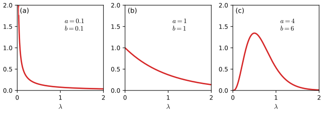
Figure 2.13 (reproduced). The gamma density for \((a,b)=(0.1,0.1)\), \((1,1)\) and \((4,6)\): \(a\) controls the shape, \(b\) the scale (mean \(a/b\)). Book: Figure 2.13, p. 100. Code: ch02_probability_distributions.py, fig2_13. Download: PDF · SVG
▶ DemoGamma prior on the precision (Figure 2.13)The gamma prior on \(\lambda\) is updated by the data; \(a_N\) grows by \(N/2\) and \(b_N\) by half the sum of squared deviations.
Unknown mean and precision: the Gaussian-gamma and Gaussian-Wishart priors
When both are unknown, the likelihood in \((\mu,\lambda)\) is proportional to \(\big[\lambda^{1/2}e^{-\lambda\mu^2/2}\big]^N\exp\{\lambda\mu\sum_nx_n\)\({}-\frac\lambda2\sum_nx_n^2\}\) (2.152). The conjugate prior must have the same dependence on \(\mu\) and \(\lambda\):
Result 2.18 (conjugate priors for the Gaussian with unknown mean and precision) (2.152)–(2.157); Exercises 2.44, 2.45
(a) The conjugate prior is the Gaussian-gamma (normal-gamma) distribution
\[ p(\mu,\lambda)=\N\big(\mu\given\mu_0,(\beta\lambda)^{-1}\big)\Gam(\lambda\given a,b).\tag{2.154} \]
Given data \(x_1,\dots,x_N\) with mean \(\bar x\) and \(S=\sum_n(x_n-\bar x)^2\), the posterior is Gaussian-gamma with
\[ \beta_N=\beta+N,\quad\mu_N=\frac{\beta\mu_0+N\bar x}{\beta+N},\quad a_N=a+\frac N2,\quad b_N=b+\frac12S+\frac{\beta N}{2(\beta+N)}(\bar x-\mu_0)^2. \]
(b) For a multivariate Gaussian with unknown precision \(\bm\Lambda\) and known mean, the conjugate prior is the Wishart distribution (2.155), \(\Wish(\bm\Lambda\given\mathbf{W},\nu)\)\[{}=B(\mathbf{W},\nu)|\bm\Lambda|^{(\nu-D-1)/2}\exp\{-\tfrac12\Tr(\mathbf{W}^{-1}\bm\Lambda)\}\]; the posterior is \(\Wish(\bm\Lambda\given\mathbf{W}_N,\nu+N)\) with \(\mathbf{W}_N^{-1}\)\({}=\mathbf{W}^{-1}\)\({}+\sum_n(\mathbf{x}_n-\bm\mu)(\mathbf{x}_n-\bm\mu)^\T\). With both unknown, the Gaussian-Wishart prior is \(\N(\bm\mu\given\bm\mu_0,(\beta\bm\Lambda)^{-1})\Wish(\bm\Lambda\given\mathbf{W},\nu)\) (2.157), also conjugate.
Proof
Form of the conjugate prior. Let the prior have the shape of the likelihood raised to a "prior sample size" \(\beta\) with free linear and constant terms \(c,d\):
\[ p(\mu,\lambda)\propto\big[\lambda^{1/2}e^{-\lambda\mu^2/2}\big]^\beta\exp\{c\lambda\mu-d\lambda\}=\exp\Big\{-\frac{\beta\lambda}2\Big(\mu-\frac c\beta\Big)^2\Big\}\lambda^{\beta/2}\exp\Big\{-\Big(d-\frac{c^2}{2\beta}\Big)\lambda\Big\}.\tag{2.153} \]
Write \(p(\mu,\lambda)=p(\mu\given\lambda)p(\lambda)\). The first factor times \(\lambda^{1/2}\) (the normalisation of a Gaussian with precision \(\beta\lambda\)) is \(\N(\mu\given c/\beta,(\beta\lambda)^{-1})\); so the remaining factor must be \(p(\lambda)\)\({}\propto\lambda^{\beta/2-1/2}\exp\{-(d-c^2/2\beta)\lambda\}\), a gamma density with \(a=\frac{1+\beta}2\) and \(b=d-\frac{c^2}{2\beta}\), and \(\mu_0=c/\beta\). Erratum. The book prints \(a=1+\beta/2\); the correct value is \((1+\beta)/2\).
Posterior (Exercise 2.44). Multiply by the likelihood. The \(\lambda\)-power is \(\lambda^{1/2}\lambda^{a-1}\lambda^{N/2}\), and the exponent is \(-\lambda\{b+\frac\beta2(\mu-\mu_0)^2\)\({}+\frac12\sum_n(x_n-\mu)^2\}\). Use \(\sum_n(x_n-\mu)^2=S+N(\mu-\bar x)^2\) and the identity
\[ \beta(\mu-\mu_0)^2+N(\mu-\bar x)^2=(\beta+N)(\mu-\mu_N)^2+\frac{\beta N}{\beta+N}(\bar x-\mu_0)^2,\qquad\mu_N=\frac{\beta\mu_0+N\bar x}{\beta+N} \]
(complete the square in \(\mu\)). The posterior is proportional to \[\lambda^{1/2}\exp\{-\frac{(\beta+N)\lambda}2(\mu-\mu_N)^2\}\cdot\lambda^{a+N/2-1}\exp\{-b_N\lambda\}\], which is \[\N(\mu\given\mu_N,((\beta+N)\lambda)^{-1})\Gam(\lambda\given a+\frac N2,b_N)\] with \(b_N\) as stated. Since \(\mu_N\) is the pooled mean of \(\beta\) pseudo-observations at \(\mu_0\) and the \(N\) data, \(\beta\) acts as a prior sample size.
Wishart (Exercise 2.45). The likelihood for the precision matrix, with known \(\bm\mu\), is \(\propto|\bm\Lambda|^{N/2}\exp\{-\tfrac12\Tr(\bm\Lambda\mathbf{S}_\mu)\}\), \(\mathbf{S}_\mu\)\({}=\sum_n(\mathbf{x}_n-\bm\mu)(\mathbf{x}_n-\bm\mu)^\T\) (2.118 in terms of \(\bm\Lambda\)). Multiplying by the Wishart prior gives \(|\bm\Lambda|^{(\nu+N-D-1)/2}\exp\{-\tfrac12\Tr((\mathbf{W}^{-1}+\mathbf{S}_\mu)\bm\Lambda)\}\), a Wishart with \(\nu+N\) degrees of freedom and scale matrix \((\mathbf{W}^{-1}+\mathbf{S}_\mu)^{-1}\). The Wishart is the multivariate generalisation of the gamma (\(D=1\), \(\nu=2a\), \(W=1/(2b)\)); its normaliser \(B(\mathbf{W},\nu)\) (2.156) and its properties are in the toolkit (Wishart). The Gaussian-Wishart posterior follows the Gaussian-gamma computation with matrices. ∎
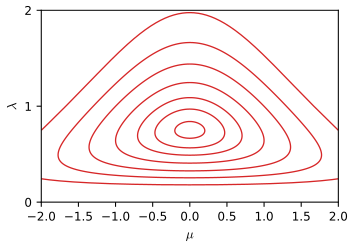
Figure 2.14 (reproduced). Contours of the Gaussian-gamma density (2.154) for \(\mu_0=0\), \(\beta=2\), \(a=5\), \(b=6\). The conditional spread of \(\mu\) is \((\beta\lambda)^{-1/2}\), so the density narrows in \(\mu\) as \(\lambda\) grows: the mean and the precision are not independent a priori. Book: Figure 2.14, p. 102. Code: ch02_probability_distributions.py, fig2_14. Download: PDF · SVG
2.3.7 Student's t-distribution
pp. 102–105 Integrating the unknown precision out of a Gaussian, with a gamma prior on it, gives a different, heavy-tailed distribution:
Result 2.19 (Student's t as an infinite mixture of Gaussians; its properties) (2.158)–(2.166); Exercises 2.46–2.50
(a) With \(\nu=2a\) and \(\lambda=a/b\), (2.158) is the Student t density
\[ \St(x\given\mu,\lambda,\nu)=\frac{\Gamma(\nu/2+1/2)}{\Gamma(\nu/2)}\Big(\frac\lambda{\pi\nu}\Big)^{1/2}\Big[1+\frac{\lambda(x-\mu)^2}\nu\Big]^{-\nu/2-1/2},\tag{2.159} \]
equivalently \(\St(x\given\mu,\lambda,\nu)\)\({}=\int_0^\infty\N(x\given\mu,(\eta\lambda)^{-1})\Gam(\eta\given\nu/2,\nu/2)\,\d\eta\) (2.160). (b) In \(D\) dimensions, \(\St(\mathbf{x}\given\bm\mu,\bm\Lambda,\nu)\)\({}=\int_0^\infty\N(\mathbf{x}\given\bm\mu,(\eta\bm\Lambda)^{-1})\Gam(\eta\given\nu/2,\nu/2)\d\eta\) (2.161) equals
\[ \St(\mathbf{x}\given\bm\mu,\bm\Lambda,\nu)=\frac{\Gamma(D/2+\nu/2)}{\Gamma(\nu/2)}\frac{|\bm\Lambda|^{1/2}}{(\pi\nu)^{D/2}}\Big[1+\frac{\Delta^2}\nu\Big]^{-D/2-\nu/2},\qquad\Delta^2=(\mathbf{x}-\bm\mu)^\T\bm\Lambda(\mathbf{x}-\bm\mu),\tag{2.162, 2.163} \]
and it is normalised. (c) \(\E[\mathbf{x}]=\bm\mu\) for \(\nu>1\), \(\cov[\mathbf{x}]=\frac\nu{\nu-2}\bm\Lambda^{-1}\) for \(\nu>2\), \(\mathrm{mode}[\mathbf{x}]=\bm\mu\) (2.164–2.166). (d) As \(\nu\to\infty\), \(\St(\mathbf{x}\given\bm\mu,\bm\Lambda,\nu)\)\({}\to\N(\mathbf{x}\given\bm\mu,\bm\Lambda^{-1})\). For \(\nu=1\) it is the Cauchy distribution.
Proof
(b) first (it contains (a) for \(D=1\)). Insert the densities into (2.161):
\[ \int_0^\infty\frac{\eta^{D/2}|\bm\Lambda|^{1/2}}{(2\pi)^{D/2}}e^{-\eta\Delta^2/2}\frac{(\nu/2)^{\nu/2}}{\Gamma(\nu/2)}\eta^{\nu/2-1}e^{-\nu\eta/2}\d\eta=\frac{|\bm\Lambda|^{1/2}(\nu/2)^{\nu/2}}{(2\pi)^{D/2}\Gamma(\nu/2)}\int_0^\infty\eta^{(D+\nu)/2-1}\exp\Big\{-\eta\frac{\nu+\Delta^2}2\Big\}\d\eta. \]
The integral is \(\Gamma(\frac{D+\nu}2)\big(\frac{\nu+\Delta^2}2\big)^{-(D+\nu)/2}\) (gamma integral, Result 2.17(a)). Collecting powers, \[\big(\frac\nu2\big)^{\nu/2}\big(\frac{\nu}2\big)^{-(D+\nu)/2}(1+\Delta^2/\nu)^{-(D+\nu)/2}(2\pi)^{-D/2}\]\({}=(\pi\nu)^{-D/2}(1+\Delta^2/\nu)^{-(D+\nu)/2}\), which is (2.162). Normalisation (Exercise 2.48): integrate (2.161) over \(\mathbf{x}\) first (allowed since everything is non-negative): for each \(\eta\) the Gaussian integrates to \(1\), leaving \(\int\Gam(\eta\given\nu/2,\nu/2)\d\eta=1\). (a) With \(D=1\), \(\Lambda=\lambda\): this is (2.159), and (2.158) is the same integral with the parameters \(a=\nu/2\), \(b=\nu/(2\lambda)\) (so \(\lambda=a/b\)): substituting \(\tau=\eta\lambda\) maps one onto the other. (This is the computation of Exercise 2.46; the result also shows that \(\St\) is the marginal for \(\mu\) in the Gaussian-gamma model.)
(c) Moments (Exercise 2.49). Given \(\eta\), \(\mathbf{x}\sim\N(\bm\mu,(\eta\bm\Lambda)^{-1})\). Then \(\E[\mathbf{x}]\)\({}=\E_\eta[\E[\mathbf{x}\given\eta]]\)\({}=\bm\mu\), and by the law of total covariance (Result 2.4) \(\cov[\mathbf{x}]\)\({}=\E_\eta[\eta^{-1}\bm\Lambda^{-1}]\)\({}+\cov_\eta(\bm\mu)\)\({}=\E[\eta^{-1}]\bm\Lambda^{-1}\). For \(\eta\sim\Gam(\nu/2,\nu/2)\), \(\E[\eta^{-1}]\)\({}=\frac{(\nu/2)^{\nu/2}}{\Gamma(\nu/2)}\int\eta^{\nu/2-2}e^{-\nu\eta/2}\d\eta\)\({}=\frac{\Gamma(\nu/2-1)}{\Gamma(\nu/2)}\frac\nu2\)\({}=\frac{\nu}{\nu-2}\) for \(\nu>2\). The mean exists when \(\E[\eta^{-1/2}]\) is finite, i.e. \(\nu>1\) (the tails of (2.162) decay as \(\|\mathbf{x}\|^{-(\nu+D)}\), so the covariance needs \(\nu>2\)). The density is a decreasing function of \(\Delta^2\), so its mode is at \(\bm\mu\).
(d) Limit (Exercises 2.47, 2.50). As \(\nu\to\infty\), \([1+\Delta^2/\nu]^{-(\nu+D)/2}\)\({}=\exp\{-\frac{\nu+D}2\ln(1+\Delta^2/\nu)\}\)\({}\to\exp\{-\Delta^2/2\}\). The prefactor tends to \((2\pi)^{-D/2}|\bm\Lambda|^{1/2}\) by Stirling: \(\Gamma(\frac{\nu+D}2)/\Gamma(\frac\nu2)\)\({}\sim(\nu/2)^{D/2}\). (More directly, \(\Gam(\eta\given\nu/2,\nu/2)\) has mean \(1\) and variance \(2/\nu\to0\), so it tends to a point mass at \(\eta=1\) and the mixture (2.161) tends to the single Gaussian \(\N(\bm\mu,\bm\Lambda^{-1})\).) For \(\nu=1\): \(\St(x\given\mu,\lambda,1)\)\({}=\frac{1}{\pi}\sqrt\lambda\,[1+\lambda(x-\mu)^2]^{-1}\), the Cauchy density, with no mean. ∎
Statistically, \(\St\) is a Gaussian whose variance is itself uncertain: a mixture of Gaussians with the same mean and different precisions, the precision \(\eta\lambda\) being drawn from a gamma. Different widths superimpose into heavy tails; \(\nu\) (the degrees of freedom) controls how heavy (Figure 2.15). See also the toolkit (Student t).
Figure 2.15 (reproduced). The t density (2.159) for \(\mu=0\), \(\lambda=1\) and \(\nu=0.1,1.0,\infty\); \(\nu\to\infty\) is the Gaussian, \(\nu=1\) the Cauchy distribution. Book: Figure 2.15, p. 103. Code: ch02_probability_distributions.py, fig2_15. Download: PDF · SVG
Filling the gap 2.5: robust fitting of a t-distribution by EM pp. 103–104, Figure 2.16
The book notes that the maximum likelihood fit of a t has no closed form and "can be found by EM". Here is the E step, which also explains the robustness.
Derivation
Treat the gamma variable \(\eta_n\) of each point (2.161) as latent. The complete-data log likelihood of one point is, up to terms in \(\nu\) alone, \(\frac D2\ln\eta_n+\frac12\ln|\bm\Lambda|\)\({}-\frac{\eta_n}2\Delta_n^2\)\({}+\ln\Gam(\eta_n\given\nu/2,\nu/2)\). Posterior of \(\eta_n\). By Bayes, \(p(\eta\given\mathbf{x}_n)\)\({}\propto\eta^{D/2}e^{-\eta\Delta_n^2/2}\eta^{\nu/2-1}e^{-\nu\eta/2}\)\({}=\eta^{(D+\nu)/2-1}e^{-\eta(\nu+\Delta_n^2)/2}\), a gamma density \(\Gam\big(\frac{D+\nu}2,\frac{\nu+\Delta_n^2}2\big)\) with mean
\[ \E[\eta_n\given\mathbf{x}_n]=\frac{\nu+D}{\nu+\Delta_n^2}. \]
M step. The terms involving \(\bm\mu\) and \(\bm\Lambda\) form a weighted Gaussian log likelihood \(\sum_n\{\frac12\ln|\bm\Lambda|\)\({}-\frac12\E[\eta_n]\Delta_n^2\}\), so \(\bm\mu\)\({}=\sum_n\E[\eta_n]\mathbf{x}_n/\sum_n\E[\eta_n]\) and \(\bm\Lambda^{-1}\)\({}=\frac1N\sum_n\E[\eta_n](\mathbf{x}_n-\bm\mu)(\mathbf{x}_n-\bm\mu)^\T\). The weight \(\E[\eta_n]\) is small for an outlier (large \(\Delta_n^2\)), so the fit down-weights distant points: this is why the t fit in Figure 2.16(b) is hardly moved by three outliers while the Gaussian (which gives every point weight one) is dragged toward them. For \(\nu\to\infty\) all weights tend to \(1\) and one recovers the Gaussian fit. (The fixed-point equations are those of Chapter 9 with a latent scale; the update of \(\nu\) has no closed form and uses a one-dimensional numerical solve.) ∎
Figure 2.16 (reproduced). Robustness of the Student t. (a) A histogram of 30 points from a Gaussian with the maximum likelihood fits of a t and a Gaussian: nearly the same. (b) The same data plus three outliers: the Gaussian fit is pulled toward them and broadened, the t fit is hardly affected. In our run, for the 30 clean points the t fit gives \(\nu\approx101\) and the Gaussian has mean \(-0.015\), sd 0.916; with the three outliers the t fit gives \(\mu=0.136\), scale 0.753, \(\nu=1.38\), while the Gaussian moves to mean 0.823, sd 2.793. Book: Figure 2.16, p. 104. Code: ch02_probability_distributions.py, fig2_16. Download: PDF · SVG
2.3.8 Periodic variables
pp. 105–110 Wind direction, time of day or the phase of a signal are periodic: \(\theta\) and \(\theta+2\pi\) are the same point. Averaging angles as ordinary numbers is meaningless (the mean of \(1^\circ\) and \(359^\circ\) is not \(180^\circ\)), and a Gaussian is not periodic. The remedy is to represent each \(\theta_n\) as a unit vector \(\mathbf{x}_n=(\cos\theta_n,\sin\theta_n)\) in the plane (Figure 2.17), whose mean is
(using the two-argument arctangent so that the quadrant is right; the common factor \(1/N\) cancels). The circular mean \(\bar\theta\) does not depend on the origin of the angle: rotating all \(\theta_n\) by \(\alpha\) rotates \(\bar{\mathbf{x}}\) by \(\alpha\). The length \(\bar r\in[0,1]\) measures concentration (\(\bar r=1\) when all angles coincide, \(\bar r=0\) when they cancel).
A periodic density is a function with \(p(\theta)\ge0\), \(\int_0^{2\pi}p(\theta)\d\theta=1\) and \(p(\theta+2\pi)=p(\theta)\) (2.170–2.172). Projecting a Gaussian onto a circle, or wrapping it around, are possible but clumsy; the von Mises distribution comes from conditioning a bivariate Gaussian \(p(x_1,x_2)\)\({}=\frac1{2\pi\sigma^2}\exp\{-\frac{(x_1-\mu_1)^2+(x_2-\mu_2)^2}{2\sigma^2}\}\) (2.173) on the unit circle \(r=1\), with \((\mu_1,\mu_2)=r_0(\cos\theta_0,\sin\theta_0)\) (2.175). In polar coordinates (2.174) the exponent on the circle is
\[ \frac1{\sigma^2}\big\{r_0\cos\theta_0\cos\theta+r_0\sin\theta_0\sin\theta\big\}+\mathrm{const}=\frac{r_0}{\sigma^2}\cos(\theta-\theta_0)+\mathrm{const}\tag{2.176} \]
(the terms \(x_1^2+x_2^2=1\) and \(\mu_1^2+\mu_2^2\) are constants), using \(\cos A\cos B+\sin A\sin B=\cos(A-B)\) (2.178). With \(m=r_0/\sigma^2\) this is
\(\theta_0\) is the mean (mode) and \(m\) the concentration, the analogue of a precision; \(I_0\) is the zeroth-order modified Bessel function of the first kind (erratum: "modified").
Result 2.20 (the von Mises distribution) (2.177)–(2.187); Exercises 2.51–2.55
(a) The normaliser is \(I_0(m)=\sum_{k\ge0}\frac{(m/2)^{2k}}{(k!)^2}\), and \(I_0'(m)=I_1(m)\) with \(I_1(m)\)\({}=\frac1{2\pi}\int_0^{2\pi}\cos\theta\,e^{m\cos\theta}\d\theta\). (b) The density has its maximum at \(\theta=\theta_0\) and its minimum at \(\theta_0+\pi\) (mod \(2\pi\)). (c) For large \(m\) it tends to a Gaussian in \(\theta-\theta_0\) with variance \(1/m\). (d) Given \(\theta_1,\dots,\theta_N\), the maximum likelihood estimates are
\[ \theta_0^{\rm ML}=\tan^{-1}\Big\{\frac{\sum_n\sin\theta_n}{\sum_n\cos\theta_n}\Big\}\ (=\bar\theta),\qquad A(m_{\rm ML})=\frac1N\sum_n\cos(\theta_n-\theta_0^{\rm ML})=\bar r,\qquad A(m)=\frac{I_1(m)}{I_0(m)}.\tag{2.184--2.187} \]
\(A\) is strictly increasing from \(0\) to \(1\), so \(m_{\rm ML}\) is the unique solution, found numerically (Figure 2.20).
(a) Normaliser. Expand \(e^{m\cos\theta}=\sum_nm^n\cos^n\theta/n!\). Over a full period \(\int_0^{2\pi}\cos^n\theta\,\d\theta=0\) for odd \(n\), and \(=2\pi\binom{2k}{k}4^{-k}\) for \(n=2k\) (write \(\cos\theta=(e^{i\theta}+e^{-i\theta})/2\); only the terms with equally many of each survive, and there are \(\binom{2k}k\) of them). Hence \(I_0(m)\)\({}=\sum_k\frac{m^{2k}}{(2k)!}\binom{2k}k4^{-k}\)\({}=\sum_k\frac{m^{2k}}{4^k(k!)^2}\), which is finite for all \(m\), so (2.179) is normalised by construction; also the integral over any interval of length \(2\pi\) is the same, by periodicity. Differentiating under the integral sign in (2.180), \(I_0'(m)=I_1(m)\).
(b) Extrema (Exercise 2.54). \(p'(\theta)=-m\sin(\theta-\theta_0)\,p(\theta)\), which vanishes exactly at \(\theta=\theta_0\) and \(\theta_0+\pi\) (mod \(2\pi\)) for \(m>0\), as \(p>0\) because \(I_0>0\). At these points \(p''=-m\cos(\theta-\theta_0)p\), equal to \(-mp<0\) at \(\theta_0\) (a maximum) and \(+mp>0\) at \(\theta_0+\pi\) (a minimum).
(c) Large \(m\) (Exercise 2.52). Put \(\xi=m^{1/2}(\theta-\theta_0)\). Then \(m\cos(\theta-\theta_0)\)\({}=m\{1-\frac{\xi^2}{2m}+O(\xi^4/m^2)\}\)\({}=m-\frac{\xi^2}2+O(m^{-1})\), so \(p\propto e^{-\xi^2/2}\) as \(m\to\infty\): a Gaussian in \(\xi\) with unit variance, i.e. in \(\theta\) with variance \(1/m\).
(d) Maximum likelihood. The log likelihood is
\[ \ln p(\mathcal{D}\given\theta_0,m)=-N\ln(2\pi)-N\ln I_0(m)+m\sum_{n=1}^N\cos(\theta_n-\theta_0).\tag{2.181} \]
\(\partial/\partial\theta_0\): \(m\sum_n\sin(\theta_n-\theta_0)=0\) (2.182). Expand with (2.183): \(\cos\theta_0\sum_n\sin\theta_n\)\({}-\sin\theta_0\sum_n\cos\theta_n\)\({}=0\), i.e. \(\tan\theta_0\)\({}=\sum_n\sin\theta_n/\sum_n\cos\theta_n\), hence (2.184) (Exercise 2.53); the second derivative \(-m\sum_n\cos(\theta_n-\theta_0)=-mN\bar r<0\) at \(\theta_0=\bar\theta\) shows this is the maximum, since \(\sum_n\cos(\theta_n-\bar\theta)\)\({}=\sum_n\cos\theta_n\cos\bar\theta\)\({}+\sin\theta_n\sin\bar\theta\)\({}=N(\bar x_1\cos\bar\theta+\bar x_2\sin\bar\theta)\)\({}=N\bar r\) by (2.168). \(\partial/\partial m\): \(-N\frac{I_0'(m)}{I_0(m)}\)\({}+\sum_n\cos(\theta_n-\theta_0)\)\({}=0\), i.e. with \(I_0'=I_1\), \(A(m)\)\({}=\frac1N\sum_n\cos(\theta_n-\theta_0^{\rm ML})\) (2.185, with the erratum that the left side is \(A(m_{\rm ML})\)); by the computation just made (this is where the sign erratum on (2.187) enters: the identity is \(\cos\theta_n\cos\theta_0^{\rm ML}\) plus \(\sin\theta_n\sin\theta_0^{\rm ML}\)) the right side is \(\bar r\), the length of the mean vector (Figure 2.17; Exercise 2.55). \(A\) is increasing: \(A(m)=\E_m[\cos(\theta-\theta_0)]\), and since the von Mises family is exponential with sufficient statistic \(\cos(\theta-\theta_0)\), \(A'(m)=\var_m[\cos(\theta-\theta_0)]>0\) (Result 2.23); \(A(0)=0\) and \(A(m)\to1\) as \(m\to\infty\). ∎
Like the Gaussian, the maximum likelihood fit matches the first sufficient moments: the fitted distribution has the same mean direction and the same mean cosine as the data. The maximum likelihood fit does not depend on where the angle is measured from. The von Mises distribution is unimodal; for multimodal circular data one uses mixtures of von Mises distributions or a circular histogram. Another periodic distribution is the wrapped Gaussian, obtained by summing a Gaussian over all shifts \(2\pi k\) (Mardia and Jupp, 2000).
Figure 2.19 (reproduced). The von Mises density for \((m,\theta_0)=(5,\pi/4)\) and \((1,3\pi/4)\), as a Cartesian plot (left) and a polar plot (right): larger \(m\) gives a narrower peak. Book: Figure 2.19, p. 108. Code: ch02_probability_distributions.py, fig2_19. Download: PDF · SVGFigure 2.20 (reproduced). The Bessel function \(I_0(m)\) (left) and \(A(m)=I_1(m)/I_0(m)\) (right). The maximum likelihood concentration is the root of \(A(m)=\bar r\). For example \(I_0(10)=2815.7\) and \(A(10)=0.9486\). In our von Mises fit to simulated angles, \(\theta_0=2.001\) and \(m=4.038\). Book: Figure 2.20, p. 109. Code: ch02_probability_distributions.py, fig2_20. Download: PDF · SVG
2.3.9 Mixtures of Gaussians
pp. 110–113 A single Gaussian cannot represent a multimodal density, such as the two clusters of the Old Faithful data (Figure 2.21). A linear combination (mixture) of \(K\) Gaussians can:
(The conditions on \(\pi_k\) make \(p\) non-negative and normalised; erratum: since each Gaussian is non-negative, \(\pi_k\ge0\) is a sufficient condition for \(p\ge0\), and normalisation then forces \(\pi_k\le1\).) The \(\pi_k\) are the mixing coefficients. Reading them as probabilities \(p(k)=\pi_k\) of choosing component \(k\), and each Gaussian as \(p(\mathbf{x}\given k)\), (2.188) is the marginal of the joint \(p(k)p(\mathbf{x}\given k)\) (2.191):
whose logarithm no longer acts on the Gaussians (it is trapped outside the sum), so there is no closed-form maximiser. It is maximised numerically, most often by the EM algorithm (Chapter 9: Section 9.2), which alternates computing the responsibilities and re-estimating the parameters from responsibility-weighted data.
Result 2.21 (moments of a mixture; two warnings) Section 2.3.9
(a) \(\E[\mathbf{x}]=\sum_k\pi_k\bm\mu_k\) and \(\cov[\mathbf{x}]\)\({}=\sum_k\pi_k\{\bm\Sigma_k+\bm\mu_k\bm\mu_k^\T\}\)\({}-\E[\mathbf{x}]\E[\mathbf{x}]^\T\), i.e. the average within-component covariance plus the covariance of the component means. (b) The log likelihood (2.193) is unbounded above: placing a component on one data point and letting its covariance shrink drives it to \(+\infty\) (the singularity). (c) The likelihood is invariant to relabelling the components, so each solution comes in \(K!\) equivalent copies.
Proof
(a) Treat the component label \(k\) as a random variable (2.191) and apply the law of total expectation and covariance of Result 2.4: \(\E[\mathbf{x}]\)\({}=\E_k[\bm\mu_k]\)\({}=\sum_k\pi_k\bm\mu_k\), and \(\cov[\mathbf{x}]\)\({}=\E_k[\bm\Sigma_k]+\cov_k[\bm\mu_k]\) where \(\cov_k[\bm\mu_k]\)\({}=\sum_k\pi_k\bm\mu_k\bm\mu_k^\T\)\({}-\E[\mathbf{x}]\E[\mathbf{x}]^\T\). (b) Take \(\bm\Sigma_1=\sigma^2\mathbf{I}\) and \(\bm\mu_1=\mathbf{x}_1\). The \(n=1\) term of (2.193) is at least \(\ln\{\pi_1(2\pi\sigma^2)^{-D/2}\}\to\infty\) as \(\sigma\to0\), while the other terms stay bounded below (they contain the other components with fixed parameters). Maximum likelihood therefore selects local maxima, not the supremum, and practical implementations guard against collapsing components (Section 9.2.1). (c) Permuting the indices of \((\pi_k,\bm\mu_k,\bm\Sigma_k)\) leaves the sum unchanged. ∎
Mixtures with enough components can approximate any continuous density to arbitrary accuracy, which is why they are the workhorse of semi-parametric density modelling (McLachlan and Peel, 2000). Their cost is the choice of \(K\); that is a model-selection problem addressed in Chapters 3, 9 and 10.
Figure 2.21 (reproduced). The Old Faithful data with contours of one maximum likelihood Gaussian (left) and of a mixture of two Gaussians (right): the second clearly describes the two clusters. Log likelihoods: \(-1289.80\) (one Gaussian) and \(-1130.26\) (two); mixing weights \((0.356,0.644)\), means \((2.04,54.48)\) and \((4.29,79.97)\). Book: Figure 2.21, p. 110. Code: ch02_probability_distributions.py, fig2_21. Download: PDF · SVGFigure 2.22 (reproduced). A one-dimensional mixture of three Gaussians: the components, each scaled by its mixing coefficient (blue), and their sum (red). Book: Figure 2.22, p. 111. Code: ch02_probability_distributions.py, fig2_22. Download: PDF · SVGFigure 2.23 (reproduced). A mixture of three Gaussians in two dimensions: (a) contours of the components, with their mixing coefficients; (b) contours of the mixture density \(p(\mathbf{x})\); (c) a surface plot of \(p(\mathbf{x})\). Data and parameters are our reconstruction. The mixture used in Figure 9.5 is read off from this figure. Book: Figure 2.23, p. 112. Code: ch02_probability_distributions.py, fig2_23. Download: PDF · SVG
2.4 The exponential family
pp. 113–120 The Bernoulli, multinomial, Gaussian, beta, gamma, Dirichlet, Wishart, von Mises and many more share one structure. A distribution of \(\mathbf{x}\) with parameters \(\bm\eta\) is in the exponential family if
where \(\bm\eta\) are the natural parameters, \(\mathbf{u}(\mathbf{x})\) the (sufficient) statistics, \(h\) a base density, and \(g(\bm\eta)\) the normaliser that makes the density integrate to one,
(a sum for discrete \(\mathbf{x}\)). The families listed above differ in \(h\), \(\mathbf{u}\), \(g\); general results proved once here then apply to all of them.
Result 2.22 (the common distributions in exponential-family form) (2.196)–(2.223); Exercises 2.56, 2.57
Distribution
Natural parameter \(\bm\eta\)
\(\mathbf{u}(x)\)
\(h(x)\)
\(g(\bm\eta)\)
Bernoulli
\(\eta=\ln\frac\mu{1-\mu}\), \(\mu=\sigma(\eta)\)
\(x\)
\(1\)
\(\sigma(-\eta)=1-\mu\)
Multinomial (\(K\) states)
\(\eta_k=\ln\mu_k\) (over-complete) or \(\eta_k=\ln\frac{\mu_k}{\mu_K}\), \(\eta_K=0\)
Bernoulli. \(p(x\given\mu)\)\({}=\mu^x(1-\mu)^{1-x}\)\({}=(1-\mu)\exp\{x\ln\frac\mu{1-\mu}\}\) (2.196, 2.197). Put \(\eta=\ln\frac\mu{1-\mu}\), so \(\mu=\frac1{1+e^{-\eta}}=\sigma(\eta)\) (the logistic sigmoid, 2.199) and \(1-\sigma(\eta)=\sigma(-\eta)\); then \(p(x\given\eta)=\sigma(-\eta)\exp(\eta x)\) (2.200–2.203).
Multinomial. \(p(\mathbf{x}\given\bm\mu)\)\({}=\prod_k\mu_k^{x_k}\)\({}=\exp\{\sum_kx_k\ln\mu_k\}\), so \(\eta_k=\ln\mu_k\), \(\mathbf{u}=\mathbf{x}\), \(h=g=1\) (2.204–2.208); but the \(\eta_k\) are constrained by \(\sum_ke^{\eta_k}=1\), and so are not free. Eliminate \(\mu_K=1-\sum_{ksoftmax, 2.213), and \(\mu_K=\big(1+\sum_je^{\eta_j}\big)^{-1}\), giving \(p(\mathbf{x}\given\bm\eta)\)\({}=\big(1+\sum_{k
Gaussian. \(\N(x\given\mu,\sigma^2)\)\({}=\frac1{(2\pi\sigma^2)^{1/2}}\exp\{-\frac{x^2}{2\sigma^2}\)\({}+\frac{\mu x}{\sigma^2}\)\({}-\frac{\mu^2}{2\sigma^2}\}\) (2.219): \(\bm\eta=(\mu/\sigma^2,-1/(2\sigma^2))\), \(\mathbf{u}=(x,x^2)\), \(h=(2\pi)^{-1/2}\) and \(g=\sigma^{-1}e^{-\mu^2/2\sigma^2}\). Writing it in \(\bm\eta\): \(\sigma^2=-1/(2\eta_2)\), \(\mu=\eta_1\sigma^2\), so \(\sigma^{-1}=(-2\eta_2)^{1/2}\) and \(\mu^2/(2\sigma^2)\)\({}=\eta_1^2\sigma^2/2\)\({}=-\eta_1^2/(4\eta_2)\), giving \(g(\bm\eta)\)\({}=(-2\eta_2)^{1/2}\exp(\eta_1^2/4\eta_2)\) (2.220–2.223). Multivariate (Exercise 2.57): \(\N(\mathbf{x}\given\bm\mu,\bm\Sigma)\)\({}=(2\pi)^{-D/2}|\bm\Lambda|^{1/2}e^{-\bm\mu^\T\bm\Lambda\bm\mu/2}\exp\{\mathbf{x}^\T\bm\Lambda\bm\mu\)\({}-\tfrac12\Tr(\bm\Lambda\mathbf{x}\mathbf{x}^\T)\}\): \(\bm\eta=(\bm\Lambda\bm\mu,-\tfrac12\bm\Lambda)\), \(\mathbf{u}=(\mathbf{x},\mathbf{x}\mathbf{x}^\T)\) (paired by \(\bm\eta^\T\mathbf{u}\)\({}=\eta_1^\T\mathbf{x}\)\({}+\Tr(\bm\eta_2^\T\mathbf{x}\mathbf{x}^\T)\)), \(h=(2\pi)^{-D/2}\), \(g\)\({}=|\)\({}-2\bm\eta_2|^{1/2}\exp\{\tfrac14\bm\eta_1^\T\bm\eta_2^{-1}\bm\eta_1\}\).
Beta, gamma, von Mises (Exercise 2.56). \(\mathrm{Beta}(\mu\given a,b)\)\({}=\frac{\Gamma(a+b)}{\Gamma(a)\Gamma(b)}\exp\{(a-1)\ln\mu\)\({}+(b-1)\ln(1-\mu)\}\); \(\Gam(\lambda\given a,b)\)\({}=\frac{b^a}{\Gamma(a)}\exp\{(a-1)\ln\lambda\)\({}-b\lambda\}\); and \(p(\theta\given\theta_0,m)\)\({}=\frac1{2\pi I_0(m)}\exp\{m\cos\theta_0\cos\theta\)\({}+m\sin\theta_0\sin\theta\}\) by (2.178), with \(m=\|\bm\eta\|\). Read off \(\bm\eta\), \(\mathbf{u}\), \(h=1\) and \(g\) as in the table (for the gamma, \(b=-\eta_2\), \(a=\eta_1+1\)). ∎
2.4.1 Maximum likelihood and sufficient statistics
pp. 116–117 Differentiate the normalisation (2.195) with respect to \(\bm\eta\):
(a) \(\E[\mathbf{u}(\mathbf{x})]=-\nabla\ln g(\bm\eta)\) and \(\cov[\mathbf{u}(\mathbf{x})]\)\({}=-\nabla\nabla^\T\ln g(\bm\eta)\) (2.300), so \(-\ln g\) is convex. (b) For i.i.d. data \(\mathbf{X}=\{\mathbf{x}_1,\dots,\mathbf{x}_N\}\) the likelihood is
\[ p(\mathbf{X}\given\bm\eta)=\Big(\prod_{n=1}^Nh(\mathbf{x}_n)\Big)g(\bm\eta)^N\exp\Big\{\bm\eta^\T\sum_{n=1}^N\mathbf{u}(\mathbf{x}_n)\Big\},\tag{2.227} \]
and its maximum satisfies the moment-matching condition
\[ -\nabla\ln g(\bm\eta_{\rm ML})=\frac1N\sum_{n=1}^N\mathbf{u}(\mathbf{x}_n),\tag{2.228} \]
i.e. the model expectation of \(\mathbf{u}\) equals its sample average. The log likelihood is concave in \(\bm\eta\), so (2.228) has at most one solution, the global maximum. (c) The data enter only through \(\sum_n\mathbf{u}(\mathbf{x}_n)\), which is a sufficient statistic: we can discard the data once it is computed, and its dimension does not grow with \(N\). As \(N\to\infty\) the right side of (2.228) tends to \(\E_{\bm\eta_0}[\mathbf{u}]\) under the true \(\bm\eta_0\), so \(\bm\eta_{\rm ML}\to\bm\eta_0\) (consistency).
Proof
(a) The first identity is derived above. For the second, differentiate \(\E[u_i]=-\partial_i\ln g\) with respect to \(\eta_j\), using \(\partial_j p(\mathbf{x}\given\bm\eta)\)\({}=p\cdot(u_j+\partial_j\ln g)\)\({}=p\,(u_j-\E[u_j])\): \(-\partial_i\partial_j\ln g\)\({}=\partial_j\E[u_i]\)\({}=\int u_i\,p\,(u_j-\E[u_j])\d\mathbf{x}\)\({}=\E[u_iu_j]-\E[u_i]\E[u_j]\). A covariance matrix is positive semi-definite, so \(-\ln g\) is convex. (b) The product (2.227) is immediate from (2.194). Taking the log, the gradient is \(N\nabla\ln g+\sum_n\mathbf{u}(\mathbf{x}_n)\); setting it to zero gives (2.228). The Hessian is \(N\nabla\nabla^\T\ln g\)\({}=-N\cov[\mathbf{u}]\preceq\mathbf{0}\), so the log likelihood is concave. (c) Factorisation (2.227) shows that the data enter the \(\bm\eta\)-dependent part only through \(\sum_n\mathbf{u}(\mathbf{x}_n)\); the strong law of large numbers gives the limit. ∎
Examples. Bernoulli: \(-\frac{d}{d\eta}\ln\sigma(-\eta)\)\({}=\sigma(\eta)\)\({}=\mu\), so (2.228) reads \(\mu_{\rm ML}=\frac1N\sum_nx_n\) (2.7). Gaussian: \(\E[x]=\mu\) and \(\E[x^2]=\mu^2+\sigma^2\) set equal to the sample averages give the usual \(\mu_{\rm ML}\) and \(\sigma^2_{\rm ML}\) (2.121, 2.122). Multinomial: \(\mu_k=m_k/N\) (2.33). So all the maximum likelihood estimates of Sections 2.1–2.3 are special cases of (2.228). The identities \(\E[\mathbf{u}]=-\nabla\ln g\) and \(\cov[\mathbf{u}]=-\nabla\nabla^\T\ln g\) also appear in the toolkit (exponential family).
2.4.2 Conjugate priors
p. 117 For any member of the family there is a conjugate prior,
the same form with \(\nu\to\nu+N\) and \(\nu\bm\chi\)\({}\to\nu\bm\chi+\sum_n\mathbf{u}(\mathbf{x}_n)\). So \(\nu\) is an effective number of prior observations and \(\bm\chi\) the mean of \(\mathbf{u}\) in them, which unifies the pseudo-observation interpretations met for the beta (\(a,b\)), Dirichlet (\(\bm\alpha\)), gamma and Gaussian priors. Written this way, the posterior mean of the expected statistic is \(\frac{\nu\bm\chi+N\bar{\mathbf{u}}}{\nu+N}\), the weighted compromise of Result 2.3 in general. For the Bernoulli, (2.229) is \(\sigma(-\eta)^\nu e^{\nu\eta\chi}\)\({}=(1-\mu)^\nu\big(\tfrac\mu{1-\mu}\big)^{\nu\chi}\)\({}=\mu^{\nu\chi}(1-\mu)^{\nu(1-\chi)}\) as a density in \(\eta\); converting to a density in \(\mu\) multiplies by \(|\d\eta/\d\mu|=1/(\mu(1-\mu))\), giving \(\mu^{\nu\chi-1}(1-\mu)^{\nu(1-\chi)-1}\), the beta distribution with \(a=\nu\chi\), \(b=\nu(1-\chi)\), \(a+b=\nu\). Conjugate priors are tractable, not necessarily right: they should be read as modelling choices whose hyperparameters are tested against prior knowledge. Other priors, where integrals are not closed form, are handled by sampling (Chapter 11).
2.4.3 Noninformative priors
pp. 117–120 When no prior knowledge is available, one wants a prior with minimal influence on the posterior. For a discrete variable with \(K\) states this is the uniform \(p=1/K\); for a continuous parameter the naive choice is a constant. Two difficulties: if the range is unbounded, a constant is not integrable (an improper prior), which is acceptable provided the posterior is proper; and a uniform density is not invariant under a non-linear change of variable. If \(p_\lambda(\lambda)=\)const and \(\lambda=\eta^2\), then \(p_\eta(\eta)\)\({}=p_\lambda(\eta^2)\cdot2\eta\)\({}\propto\eta\) (2.231), which is not constant. Two classes of parameters have a natural uninformative prior fixed by an invariance requirement.
Result 2.24 (location and scale parameters; non-informative priors) (2.232)–(2.240); Exercise 2.59
(a) Location. If \(p(x\given\mu)=f(x-\mu)\) (2.232), the only prior invariant under translation \(\hat x=x+c\) is \(p(\mu)=\)const. (b) Scale. If \(p(x\given\sigma)=\frac1\sigma f(x/\sigma)\) (2.236), with \(f\) normalised, the only prior invariant under rescaling \(\hat x=cx\) is \(p(\sigma)\propto1/\sigma\), equivalently \(p(\ln\sigma)=\)const. (c) The Gaussian \(\N(x\given\mu,\sigma^2)\) has \(\mu\) as a location and \(\sigma\) as a scale parameter, so its non-informative prior is \(p(\mu,\sigma)\propto1/\sigma\).
Proof
(a) Under \(\hat x=x+c\), the density of \(\hat x\) is \(f(\hat x-\hat\mu)\) with \(\hat\mu=\mu+c\): same functional form, so the problem is unchanged and the prior on \(\hat\mu\) must be the same function as on \(\mu\). Equal probability for the interval \([A,B]\) before and \([A-c,B-c]\) after: \(\int_A^Bp(\mu)\d\mu\)\({}=\int_{A-c}^{B-c}p(\mu)\d\mu\)\({}=\int_A^Bp(\mu-c)\d\mu\) (2.234) for all \(A,B\), so \(p(\mu-c)=p(\mu)\) for all \(c\) (2.235): \(p\) is constant. (An example of an improper prior; the Gaussian prior of Section 2.3.6 with \(\sigma_0^2\to\infty\) approaches it: (2.141) and (2.142) become \(\mu_N\to\mu_{\rm ML}\) and \(\sigma_N^2\to\sigma^2/N\).)
(b) Normalisation of (2.236) (Exercise 2.59): with \(y=x/\sigma\), \(\int\frac1\sigma f(x/\sigma)\d x=\int f(y)\d y=1\), so the scale family is normalised if \(f\) is. Under \(\hat x=cx\), \(\hat\sigma=c\sigma\): \(p(\hat x\given\hat\sigma)\)\({}=\frac1{\hat\sigma}f(\hat x/\hat\sigma)\), the same form, so invariance requires \(\int_A^Bp(\sigma)\d\sigma\)\({}=\int_{A/c}^{B/c}p(\sigma)\d\sigma\)\({}=\int_A^Bp(\tfrac1c\sigma)\tfrac1c\d\sigma\) (2.238). Hence \(p(\sigma)=\frac1cp(\sigma/c)\) for all \(c>0\); taking \(c=\sigma\) gives \(p(\sigma)=\frac1\sigma p(1)\propto1/\sigma\) (2.239). Then \(p(\ln\sigma)=p(\sigma)\sigma=\)const: the scale prior is flat in \(\ln\sigma\). It is again improper, over both \((0,1)\) and \((1,\infty)\).
(c) \(\N(x\given\mu,\sigma^2)\)\({}=\frac1\sigma f\big(\frac{x-\mu}\sigma\big)\) with \(f(y)=(2\pi)^{-1/2}e^{-y^2/2}\) (2.240). In terms of the precision \(\lambda=\sigma^{-2}\), \(p(\lambda)=p(\sigma)|\d\sigma/\d\lambda|\): with \(\sigma=\lambda^{-1/2}\), \(|\d\sigma/\d\lambda|=\frac12\lambda^{-3/2}\) and \(p(\sigma)\propto\lambda^{1/2}\), so \(p(\lambda)\propto\lambda^{-1}\), which is the gamma prior with \(a_0=b_0=0\) of Section 2.3.6 (the posterior (2.150, 2.151) is then proper for \(N\ge1\) when \(\sum_n(x_n-\mu)^2>0\)). ∎
Filling the gap 2.6: Jeffreys' prior, an invariance principle that contains both rules p. 118, (Jeffreys, 1946)
The book mentions Jeffreys without details. The invariant construction generalises (a) and (b).
Derivation
Let \(I(\theta)\)\({}=\E_{x\given\theta}\big[(\partial_\theta\ln p(x\given\theta))^2\big]\) be the Fisher information. Under a reparametrisation \(\theta=\theta(\phi)\), the chain rule gives \(\partial_\phi\ln p\)\({}=\partial_\theta\ln p\cdot\frac{\d\theta}{\d\phi}\), so \(I(\phi)\)\({}=I(\theta)\big(\frac{\d\theta}{\d\phi}\big)^2\). The prior \(p(\theta)\propto\sqrt{I(\theta)}\) therefore transforms like a density: \(p(\phi)\)\({}=p(\theta)\big|\frac{\d\theta}{\d\phi}\big|\)\({}\propto\sqrt{I(\theta)}\big|\frac{\d\theta}{\d\phi}\big|\)\({}=\sqrt{I(\phi)}\), the same rule in the new parametrisation (invariance under all smooth reparametrisations, not only translations and scalings). Examples: for a location family \(f(x-\mu)\), \(I(\mu)=\int f'^2/f\) is constant, so \(p(\mu)\propto1\); for the Gaussian scale \(\sigma\) (mean known), \(\partial_\sigma\ln\N\)\({}=-\frac1\sigma+\frac{(x-\mu)^2}{\sigma^3}\), so \(I(\sigma)=\sigma^{-2}\E[(z^2-1)^2]=2/\sigma^2\) (\(z\) standard normal, \(\E[(z^2-1)^2]=3-2+1=2\)) and \(p(\sigma)\propto1/\sigma\); for the Bernoulli, \(I(\mu)=\frac1{\mu(1-\mu)}\), so \(p(\mu)\)\({}\propto\mu^{-1/2}(1-\mu)^{-1/2}\)\({}=\mathrm{Beta}(\mu\given\tfrac12,\tfrac12)\), between the "Haldane" prior \(\mathrm{Beta}(0,0)\) and the uniform \(\mathrm{Beta}(1,1)\). ∎
2.5 Nonparametric methods
pp. 120–127 The parametric models above assume a functional form with a fixed number of parameters. If the true density has another shape (several modes, say), the fit can be poor. Nonparametric methods make few assumptions about the form; the number of parameters then grows with the data. We estimate \(p(\mathbf{x})\) from \(N\) i.i.d. observations \(\mathbf{x}_1,\dots,\mathbf{x}_N\) and begin with the histogram.
Histograms. Divide the range of a one-dimensional variable into bins of width \(\Delta_i\), count the \(n_i\) points in bin \(i\), and set the density constant within the bin:
Result 2.25 (the histogram is the maximum likelihood piecewise-constant density) (2.241), Exercise 2.60
Among densities that are constant, \(h_i\), on fixed regions of volume \(\Delta_i\), the likelihood of the data is maximised by \(h_i=n_i/(N\Delta_i)\).
Proof
The log likelihood is \(\sum_in_i\ln h_i\) (each of the \(n_i\) points in region \(i\) contributes \(\ln h_i\)). Maximise it subject to \(\sum_ih_i\Delta_i=1\) with a multiplier: \(\sum_in_i\ln h_i+\lambda(\sum_ih_i\Delta_i-1)\). The derivative with respect to \(h_i\) is \(n_i/h_i+\lambda\Delta_i=0\), so \(h_i=-n_i/(\lambda\Delta_i)\). Multiplying by \(\Delta_i\) and summing, \(1=-N/\lambda\), so \(\lambda=-N\) and \(h_i=n_i/(N\Delta_i)\). The objective is concave on the constraint set, so this is the global maximum. ∎
A histogram is convenient (the data can be discarded after binning) but has three weaknesses: the estimate is discontinuous at the bin edges, the number of bins grows as \(M^D\) with the dimension \(D\) when each axis is divided into \(M\) intervals (the curse of dimensionality, Section 1.4), and the bin width \(\Delta\) (a smoothing parameter) must be tuned: too small a width gives a spiky estimate, too large a width hides structure (Figure 2.24).
Figure 2.24 (reproduced). Histogram density estimates of 50 points drawn from the density shown in green, for bin widths \(\Delta=0.04\) (too spiky), \(0.08\) (reasonable) and \(0.25\) (too smooth). Book: Figure 2.24, p. 121. Code: ch02_probability_distributions.py, fig2_24. Download: PDF · SVG
Filling the gap 2.7: the local estimate \(p(\mathbf{x})\approx K/(NV)\) pp. 121–122, (2.242)–(2.246)
Both kernel and nearest-neighbour estimators rest on one idea, which the book states in two sentences. Here it is with the approximations made explicit.
Derivation
Let \(\mathcal{R}\) be a small region containing \(\mathbf{x}\). The probability mass of \(\mathcal{R}\) is \(P=\int_{\mathcal{R}}p(\mathbf{y})\d\mathbf{y}\) (2.242). If \(N\) points are drawn independently, the number \(K\) falling in \(\mathcal{R}\) is binomial, \(\mathrm{Bin}(K\given N,P)\)\({}=\binom NKP^K(1-P)^{N-K}\) (2.243; erratum: the exponent of \(1-P\) is \(N-K\)). By Result 2.1, \(\E[K/N]=P\) and \(\var[K/N]=P(1-P)/N\). Two approximations:
(i) For large \(N\) the fraction \(K/N\) is sharply concentrated at \(P\) (relative standard deviation \(\sqrt{(1-P)/(NP)}\to0\)), so \(K\approx NP\) (2.244). (ii) For a small region over which \(p\) is roughly constant, \(P\approx p(\mathbf{x})V\) (2.245), with \(V\) the volume of \(\mathcal{R}\). Combining,
The two assumptions pull in opposite directions: (i) wants \(\mathcal{R}\) large enough to hold many points (\(NP\gg1\)), (ii) wants it small enough that \(p\) is nearly constant. Fixing \(V\) and counting \(K\) gives kernel methods; fixing \(K\) and finding \(V\) gives nearest-neighbour methods. Both are consistent in the sense of Section 2.5.3 if \(V\to0\) while \(NV\to\infty\) (resp. \(K\to\infty\) while \(K/N\to0\)). ∎
2.5.1 Kernel density estimators
pp. 122–124 Take \(\mathcal{R}\) to be a hypercube of side \(h\) centred at \(\mathbf{x}\), and define the Parzen window \(k(\mathbf{u})=1\) if \(|u_i|\le\tfrac12\) for all \(i=1,\dots,D\), and \(0\) otherwise (2.247). Then \(k((\mathbf{x}-\mathbf{x}_n)/h)\) is \(1\) exactly when \(\mathbf{x}_n\) lies in the cube centred at \(\mathbf{x}\), so
keeps \(p\) non-negative and normalised: \(\int\frac1{h^D}k(\frac{\mathbf{x}-\mathbf{x}_n}h)\d\mathbf{x}\)\({}=\int k(\mathbf{u})\d\mathbf{u}\)\({}=1\) for each \(n\), so \(\int p=1\). The Gaussian kernel gives
(erratum: the exponent in the normaliser is \(D/2\)), a mixture of \(N\) equally weighted Gaussians centred at the data, each with covariance \(h^2\mathbf{I}\). The bandwidth \(h\) is a smoothing parameter (Figure 2.25): small \(h\) reproduces noise, large \(h\) over-smooths. The price: all \(N\) data points must be stored and each evaluation costs \(O(N)\). Choosing \(h\) by maximum likelihood fails: the likelihood of the training data is maximised by \(h\to0\) (each point's own kernel contributes \(\frac1N(2\pi h^2)^{-D/2}\to\infty\)), the same singularity as for mixtures. One instead maximises the leave-one-out likelihood \(\sum_n\ln\big\{\frac1{N-1}\sum_{m\ne n}K_h(\mathbf{x}_n-\mathbf{x}_m)\big\}\), or the likelihood on held-out data.
Figure 2.25 (reproduced). Gaussian kernel density estimates (2.250) of the data of Figure 2.24 for \(h=0.005\) (noisy), \(0.07\) (good) and \(0.2\) (over-smoothed), with the true density in green. Book: Figure 2.25, p. 124. Code: ch02_probability_distributions.py, fig2_25. Download: PDF · SVG
Result 2.26 (bias, variance and consistency of the kernel density estimator) Section 2.5.1; Parzen (1962), Rosenblatt (1956)
Let \(D=1\), \(\hat p(x)\)\({}=\frac1N\sum_n\frac1hk\big(\frac{x-x_n}h\big)\), with a symmetric kernel, \(\mu_2=\int u^2k(u)\d u<\infty\) and \(R(k)=\int k(u)^2\d u<\infty\), and a twice continuously differentiable density \(p\). Then, as \(h\to0\) and \(Nh\to\infty\),
\[ \E[\hat p(x)]-p(x)=\tfrac12h^2\mu_2\,p''(x)+o(h^2),\qquad\var[\hat p(x)]=\frac{R(k)\,p(x)}{Nh}+o\Big(\frac1{Nh}\Big). \]
Hence \(\hat p(x)\to p(x)\) in mean square (consistency), and the bandwidth minimising the asymptotic mean squared error is \(h^\star\propto N^{-1/5}\), giving an error of order \(N^{-4/5}\). In \(D\) dimensions the same argument gives \(h^\star\propto N^{-1/(D+4)}\) and error \(N^{-4/(D+4)}\).
Proof
Bias. By independence, \(\E[\hat p(x)]\)\({}=\E\big[\frac1hk\big(\frac{x-X}h\big)\big]\)\({}=\int\frac1hk\big(\frac{x-y}h\big)p(y)\d y\)\({}=\int k(u)\,p(x-hu)\d u\) (substituting \(y=x-hu\)). Taylor-expand \(p(x-hu)\)\({}=p(x)-hu\,p'(x)+\tfrac12h^2u^2p''(x)+o(h^2)\), and use \(\int k=1\), \(\int uk=0\) (symmetry): \(\E\hat p(x)=p(x)+\tfrac12h^2\mu_2p''(x)+o(h^2)\).
Variance. The \(N\) terms are independent and identically distributed, so \(\var[\hat p(x)]\)\({}=\frac1N\var\big[\frac1hk\big(\frac{x-X}h\big)\big]\)\({}=\frac1N\big\{\E[h^{-2}k^2]\)\({}-(\E[h^{-1}k])^2\big\}\). Now \(\E[h^{-2}k^2((x-X)/h)]\)\({}=h^{-1}\int k(u)^2p(x-hu)\d u\)\({}=h^{-1}\{R(k)p(x)+o(1)\}\), and \((\E[h^{-1}k])^2=p(x)^2+o(1)\) is bounded, so \(\var\hat p(x)=\frac{R(k)p(x)}{Nh}+O(1/N)\).
Consistency. The mean squared error is bias squared plus variance:
\[ \mathrm{MSE}(h)\approx\tfrac14h^4\mu_2^2p''(x)^2+\frac{R(k)p(x)}{Nh}. \]
Both terms tend to zero when \(h\to0\) and \(Nh\to\infty\) (the first needs the window to shrink so the bias vanishes, the second needs enough points in the window to average the noise away): this is the pair of conditions of the Parzen–Rosenblatt theorem, and it is the nonparametric version of the compromise of approximations (i) and (ii) in Filling the gap 2.7. Convergence in mean square implies convergence in probability. Optimal \(h\). Write \(\mathrm{MSE}=Ah^4+B/h\) with \(A=\frac14\mu_2^2p''^2\), \(B=R(k)p/N\). Setting the derivative to zero, \(4Ah^3=B/h^2\), \(h^\star=(B/4A)^{1/5}\propto N^{-1/5}\), and \(\mathrm{MSE}(h^\star)\)\({}=5A(h^\star)^4\)\({}\propto N^{-4/5}\). In \(D\) dimensions the variance term is \(R(k)p/(Nh^D)\) and the bias term is unchanged, so \(h^{\star}\propto N^{-1/(D+4)}\) and the best error is \(N^{-4/(D+4)}\): the rate deteriorates with dimension (the curse of dimensionality again). For the Gaussian kernel, \(\mu_2=1\) and \(R(k)=1/(2\sqrt\pi)\). ∎
The tension is visible in Figures 2.24 and 2.25: small \(h\) has low bias and high variance; large \(h\) has high bias and low variance (compare the bias–variance decomposition of Section 3.2). The same analysis for histograms gives the best bin width \(\propto N^{-1/3}\) and error \(\propto N^{-2/3}\) (Scott, 1979): kernels converge faster than histograms because they are smoother.
2.5.2 Nearest-neighbour methods
pp. 124–127 A fixed bandwidth is a problem when the density varies strongly: a width that suits the dense regions gives a noisy estimate in the sparse ones, and a width that suits the sparse regions over-smooths the dense ones. Nearest-neighbour estimation adapts the volume: fix \(K\) and, around the point \(\mathbf{x}\), grow a sphere until it contains exactly \(K\) data points; with \(V\) its volume, \(p(\mathbf{x})=K/(NV)\) (2.246). Here \(K\) is the smoothing parameter (Figure 2.26): small \(K\) is noisy, large \(K\) is smooth.
Figure 2.26 (reproduced). \(K\)-nearest-neighbour density estimates of the data of Figures 2.24 and 2.25 for \(K=1,5,30\) (true density in green). Book: Figure 2.26, p. 125. Code: ch02_probability_distributions.py, fig2_26. Download: PDF · SVG
▶ DemoK nearest neighbours (Figure 2.26)Raise \(K\) from 1: the estimate has a spike at every data point for \(K=1\) and becomes a smooth bump for large \(K\).
▶ DemoMixture of Gaussians dataCompare the histogram, the kernel estimate and the \(K\)-nearest-neighbour estimate on the same bimodal sample, and with the true mixture density.
Result 2.27 (the nearest-neighbour density model is not a density) p. 124, Exercise 2.61
The \(K\)-nearest-neighbour density estimate \(\hat p(\mathbf{x})=K/(NV_K(\mathbf{x}))\) has an infinite integral over \(\R^D\), so it is an improper distribution.
Proof
Let \(r_K(\mathbf{x})\) be the distance from \(\mathbf{x}\) to its \(K\)-th nearest data point and \(V_K(\mathbf{x})=c_Dr_K(\mathbf{x})^D\), with \(c_D\) the volume of the unit ball. Let \(\rho=\max_n\|\mathbf{x}_n\|\). For \(\|\mathbf{x}\|>2\rho\) every data point is within \(\|\mathbf{x}\|+\rho\le\tfrac32\|\mathbf{x}\|\) of \(\mathbf{x}\), hence \(r_K(\mathbf{x})\le\frac32\|\mathbf{x}\|\) and \(\hat p(\mathbf{x})\)\({}\ge\frac{K}{Nc_D(3/2)^D\|\mathbf{x}\|^D}\). In polar coordinates the integral over \(\|\mathbf{x}\|>2\rho\) is at least \(\text{const}\int_{2\rho}^\infty\frac{r^{D-1}}{r^D}\d r\)\({}=\text{const}\int_{2\rho}^\infty\frac{\d r}{r}\)\({}=\infty\). (For \(D=1\): \(\hat p\sim K/(2N|x|)\) in the tails.) ∎
The estimate also has a cusp at every data point and its tails decay too slowly, so it is rarely used for density estimation itself; its value is that it leads to a classifier.
The \(K\)-nearest-neighbour classifier
Apply the density estimate to each class, with data \(N_k\) in class \(\mathcal{C}_k\) (\(\sum_kN_k=N\)). Draw a sphere around the query point \(\mathbf{x}\) that contains \(K\) points of any class, volume \(V\), of which \(K_k\) belong to \(\mathcal{C}_k\). Then
To minimise the misclassification rate, assign \(\mathbf{x}\) to the class with the largest posterior, i.e. the majority class among its \(K\) nearest neighbours (ties broken at random). For \(K=1\) every point is assigned the class of its nearest training point, and the decision regions are the union of the Voronoi cells of the training points (Figure 2.27b). \(K\) smooths the boundary (Figure 2.28): \(K=1\) fits the training data perfectly (training error zero) and has a complicated boundary with isolated islands; large \(K\) gives smooth boundaries and eventually (\(K=N\)) always predicts the largest class. \(K\) is best chosen by cross-validation. Training costs nothing but prediction requires a search through the stored data (reduced by \(k\)-d trees or similar), and the distance measure matters: the features should be scaled.
Figure 2.27 (reproduced). (a) In the \(K\)-nearest-neighbour classifier a new point (black diamond) takes the majority class of its \(K\) nearest training points (here \(K=3\)). (b) For \(K=1\) the decision regions are the Voronoi cells of the training points. Book: Figure 2.27, p. 126. Code: ch02_probability_distributions.py, fig2_27. Download: PDF · SVGFigure 2.28 (reproduced). \(K\)-nearest-neighbour classification of the plane for 200 points from the oil flow data (variables \(x_6\) against \(x_7\); classes laminar, annular, homogeneous), for \(K=1,3,31\): the boundary is complex for \(K=1\) and smooth for \(K=31\). Book: Figure 2.28, p. 126. Code: ch02_probability_distributions.py, fig2_28. Download: PDF · SVG
▶ DemoNearest-neighbour classification (Section 2.5.2)Move \(K\) from 1 upward; the decision regions change from Voronoi cells to smooth boundaries, and the readout shows the training and test error. In the demo's data the Bayes error is 0.1218, the bound 0.214, and 1-NN with 40 training points per class has test error 0.168.
2.5.3 Consistency and the Cover–Hart bound
(Not a separate section of the book: the theory behind pp. 124–127.) How good can a nearest-neighbour rule be? The Bayes error \(R^\star\)\({}=\E_{\mathbf{x}}[\min_k\{1-p(\mathcal{C}_k\given\mathbf{x})\}]\) is the smallest error any classifier can attain. Cover and Hart (1967) showed that with an unlimited training set the 1-nearest-neighbour rule is at most twice as bad.
Result 2.28 (Cover–Hart bound for the nearest-neighbour classifier) Cover and Hart (1967)
Let the classes have posteriors \(\eta_k(\mathbf{x})\)\({}=p(\mathcal{C}_k\given\mathbf{x})\), continuous in \(\mathbf{x}\), and let \(R_{\rm NN}\) be the asymptotic (\(N\to\infty\)) error of the 1-NN rule. Then for two classes
\[ R^\star\le R_{\rm NN}\le2R^\star(1-R^\star)\le2R^\star, \]
and for \(C\) classes \(R_{\rm NN}\)\({}\le R^\star\big(2-\tfrac{C}{C-1}R^\star\big)\).
Proof
Step 1: the neighbour becomes the point. Fix \(\mathbf{x}\) in the support of \(p\) and \(\varepsilon>0\). The ball \(B(\mathbf{x},\varepsilon)\) has probability \(q>0\), and the probability that none of \(N\) independent points falls in it is \((1-q)^N\to0\) (summably, so almost surely). Hence the nearest neighbour \(\mathbf{x}'_N\) of \(\mathbf{x}\) converges to \(\mathbf{x}\), and by continuity \(\eta_k(\mathbf{x}'_N)\to\eta_k(\mathbf{x})\).
Step 2: the conditional error. A test point with input \(\mathbf{x}\) has label \(y\sim\eta(\mathbf{x})\) and its neighbour has label \(y'\sim\eta(\mathbf{x}'_N)\), independent of \(y\) given the inputs. In the limit both are drawn from \(\eta(\mathbf{x})\) independently, so the 1-NN rule errs, i.e. \(y\ne y'\), with probability \(r(\mathbf{x})=1-\sum_k\eta_k(\mathbf{x})^2\), and \(R_{\rm NN}=\E_{\mathbf{x}}[r(\mathbf{x})]\). The Bayes rule errs with probability \(r^\star(\mathbf{x})=1-\max_k\eta_k(\mathbf{x})\), and \(R^\star=\E[r^\star]\).
Step 3: two classes. With \(\eta_1=\eta\), \(\eta_2=1-\eta\): \(r\)\({}=1-\eta^2-(1-\eta)^2\)\({}=2\eta(1-\eta)\)\({}=2r^\star(1-r^\star)\), since \(r^\star=\min(\eta,1-\eta)\). So \(R_{\rm NN}=2\E[r^\star]-2\E[(r^\star)^2]\). Because \(2r^\star(1-r^\star)\ge r^\star\) when \(r^\star\le\tfrac12\) (always), \(R_{\rm NN}\ge R^\star\). By Jensen's inequality (\(\E[r^{\star2}]\ge(\E r^\star)^2\)), \(R_{\rm NN}\)\({}\le2R^\star-2R^{\star2}\)\({}=2R^\star(1-R^\star)\).
Step 4: \(C\) classes. Let \(\eta_{\max}=1-r^\star\). The remaining mass \(r^\star\) is spread over \(C-1\) classes, and \(\sum_{k\ne\max}\eta_k^2\ge(r^\star)^2/(C-1)\) (Cauchy–Schwarz, equality when the rest is uniform). So \(r\)\({}\le1-(1-r^\star)^2-\frac{(r^\star)^2}{C-1}\)\({}=2r^\star-\frac{C}{C-1}(r^\star)^2\). Taking expectations and using Jensen again, \(R_{\rm NN}\le2R^\star-\frac{C}{C-1}R^{\star2}\). ∎
Numerical check (course code, one-dimensional Gaussian classes with unit separation): \(R^\star=0.3085\), 1-NN error \(0.4055\), bound \(2R^\star(1-R^\star)=0.4267\). Interpretation: if the Bayes error is \(R^\star=0.1\), the nearest-neighbour rule has asymptotic error at most \(0.18\); if \(R^\star\) is small it is at most about twice as large. The rule needs no model but converges only as the number of points grows, and in high dimensions very slowly. Larger \(K\) does better:
Result 2.29 (consistency of the \(K\)-nearest-neighbour classifier, idea) Stone (1977)
If \(K=K_N\to\infty\) and \(K_N/N\to0\), the \(K\)-nearest-neighbour rule has risk converging to the Bayes risk \(R^\star\), for every distribution (Stone, 1977). The two conditions are the counterparts of \(Nh\to\infty\) and \(h\to0\) for kernels.
Proof idea for continuous posteriors
Fix \(\mathbf{x}\) and \(\varepsilon>0\). Since \(K/N\to0\), the ball around \(\mathbf{x}\) containing the \(K\) nearest points has probability mass about \(K/N\to0\), hence radius \(\to0\), and by continuity of \(\eta_k\) all its points have posteriors within \(\varepsilon\) of \(\eta_k(\mathbf{x})\). The labels of the \(K\) neighbours are then (almost) independent draws with probabilities within \(\varepsilon\) of \(\eta_k(\mathbf{x})\), so \(K_k/K\) has mean within \(\varepsilon\) of \(\eta_k(\mathbf{x})\) and variance at most \(1/(4K)\to0\) because \(K\to\infty\). Hence \(K_k/K\to\eta_k(\mathbf{x})\) in probability, the majority class is the Bayes class wherever the largest posterior is unique, and the excess risk tends to zero (the excess is controlled by the points where the two largest posteriors are within \(2\varepsilon\), whose probability tends to zero with \(\varepsilon\)). The proof for arbitrary distributions requires Stone's lemma and is not reproduced here. ∎
This closes the circle with the start of the chapter: the parametric families of Sections 2.1–2.4 estimate with few numbers and risk bias if the form is wrong; the nonparametric estimators of this section are consistent for any distribution at the price of storing the data and of slow convergence in high dimensions. Bayesian and mixture approaches (Chapters 9–10) sit between.
Exercises
All 61 exercises of Chapter 2 (Bishop, 2006, pp. 126–136), restated in my own words, with complete solutions (hidden). Stars give the book's difficulty and "www" marks the exercises with official solutions. Many exercises are the derivations of the results above; their solutions give the argument and link to the full version.
Exercise 2.1 (★, www). Show that the Bernoulli distribution (2.2) satisfies \(\sum_{x=0}^1p(x\given\mu)=1\), \(\E[x]=\mu\), \(\var[x]=\mu(1-\mu)\), and that its entropy is \(\mathrm H[x]=-\mu\ln\mu-(1-\mu)\ln(1-\mu)\).
Solution
Proved in Result 2.1(a): the two probabilities are \(1-\mu\) and \(\mu\); \(\E[x]=\mu\); \(x^2=x\) gives \(\E[x^2]=\mu\) and \(\var[x]=\mu-\mu^2\); and \(\mathrm H\)\({}=-\sum_xp\ln p\)\({}=-(1-\mu)\ln(1-\mu)-\mu\ln\mu\).
Exercise 2.2 (★★). For the \(\{-1,+1\}\) coding \(p(x\given\mu)\)\({}=\big(\frac{1-\mu}2\big)^{(1-x)/2}\big(\frac{1+\mu}2\big)^{(1+x)/2}\), \(\mu\in[-1,1]\), show normalisation and evaluate the mean, variance and entropy.
Solution
For \(x=-1\) the exponents are \(1\) and \(0\), giving \(p=\frac{1-\mu}2\); for \(x=+1\) they are \(0\) and \(1\), giving \(\frac{1+\mu}2\). The sum is \(\frac{1-\mu}2+\frac{1+\mu}2=1\), and both are in \([0,1]\) for \(\mu\in[-1,1]\). Mean: \(\E[x]=(-1)\frac{1-\mu}2+(+1)\frac{1+\mu}2=\mu\). Since \(x^2=1\), \(\E[x^2]=1\) and \(\var[x]=1-\mu^2\). Entropy: \(\mathrm H\)\({}=-\frac{1-\mu}2\ln\frac{1-\mu}2\)\({}-\frac{1+\mu}2\ln\frac{1+\mu}2\), which is the Bernoulli entropy at \(\mu'=(1+\mu)/2\) (the two codings are related by \(x'=(x+1)/2\), \(\mu'=(\mu+1)/2\)).
Exercise 2.3 (★★, www). Prove that the binomial distribution (2.9) is normalised: (i) \(\binom Nm+\binom N{m-1}=\binom{N+1}m\); (ii) the binomial theorem \((1+x)^N=\sum_m\binom Nmx^m\) by induction; (iii) \(\sum_m\binom Nm\mu^m(1-\mu)^{N-m}=1\).
Solution
Full argument in Result 2.1(b). In brief: (i) put the two fractions over the common denominator \(m!(N+1-m)!\): the numerators add to \(N!\,[(N-m+1)+m]=(N+1)!\). (ii) For \(N=1\) it is \(1+x\). Assuming it for \(N\), multiply by \((1+x)\) and shift the index of the second sum: \((1+x)^{N+1}\)\({}=\sum_m[\binom Nm+\binom N{m-1}]x^m\)\({}=\sum_m\binom{N+1}mx^m\) by (i), with \(\binom N{-1}=\binom N{N+1}=0\). (iii) Factor \((1-\mu)^N\) and apply (ii) with \(x=\mu/(1-\mu)\): \((1-\mu)^N(1+\frac\mu{1-\mu})^N=1\).
Exercise 2.4 (★★). Show that the mean (2.11) and variance (2.12) of the binomial distribution follow by differentiating the normalisation (2.264) once and twice with respect to \(\mu\).
Solution
Let \(B_m=\binom Nm\mu^m(1-\mu)^{N-m}\). Then \(\partial_\mu B_m=B_m\frac{m-N\mu}{\mu(1-\mu)}\) (the log derivative is \(\frac m\mu-\frac{N-m}{1-\mu}\)). Differentiating \(\sum_mB_m=1\): \(\sum_m(m-N\mu)B_m=0\), so \(\E[m]=N\mu\). Differentiating this identity again, \(\sum_m[-NB_m+(m-N\mu)\partial_\mu B_m]=0\), i.e. \(-N+\frac1{\mu(1-\mu)}\sum_m(m-N\mu)^2B_m=0\), so \(\var[m]=N\mu(1-\mu)\). (Result 2.1.)
Exercise 2.5 (★★, www). Prove that the beta distribution (2.13) is normalised, i.e. \(\int_0^1\mu^{a-1}(1-\mu)^{b-1}\d\mu\)\({}=\Gamma(a)\Gamma(b)/\Gamma(a+b)\), by the steps suggested in the book.
Solution
Write \(\Gamma(a)\Gamma(b)\)\({}=\int_0^\infty\!\!\int_0^\infty e^{-x-y}x^{a-1}y^{b-1}\d y\,\d x\). (1) Bring the \(y\)-integral inside and substitute \(t=x+y\) for fixed \(x\): \(\int_0^\infty\!\int_x^\infty e^{-t}x^{a-1}(t-x)^{b-1}\d t\,\d x\). (2) The region is \(0\le x\le t\); swap the order: \(\int_0^\infty e^{-t}\int_0^tx^{a-1}(t-x)^{b-1}\d x\,\d t\). (3) For fixed \(t\) put \(x=t\mu\): the inner integral is \(t^{a+b-1}\int_0^1\mu^{a-1}(1-\mu)^{b-1}\d\mu\). (4) The \(t\)-integral \(\int_0^\infty e^{-t}t^{a+b-1}\d t=\Gamma(a+b)\), giving the claim. See Result 2.2.
Exercise 2.6 (★). Show that the mean, variance and mode of the beta distribution are \(\frac a{a+b}\), \(\frac{ab}{(a+b)^2(a+b+1)}\), \(\frac{a-1}{a+b-2}\).
Solution
With \(B(a,b)=\Gamma(a)\Gamma(b)/\Gamma(a+b)\), \(\E[\mu^k]=B(a+k,b)/B(a,b)\); then \(\Gamma(x+1)=x\Gamma(x)\) gives \(\E[\mu]=\frac a{a+b}\) and \(\E[\mu^2]=\frac{a(a+1)}{(a+b)(a+b+1)}\), whence the variance. The mode solves \(\frac{a-1}\mu=\frac{b-1}{1-\mu}\) (for \(a,b>1\)). Details in Result 2.2.
Exercise 2.7 (★★). A binomial variable has a beta prior on \(\mu\) and \(m\) ones and \(l\) zeros are observed. Show that the posterior mean of \(\mu\) lies between the prior mean and the maximum likelihood estimate. (Erratum: the book says mean of \(x\).)
Solution
The posterior is \(\mathrm{Beta}(\mu\given a+m,b+l)\), mean \(\frac{a+m}{a+b+m+l}\). With \(N=m+l\) and \(\lambda=\frac{a+b}{a+b+N}\in(0,1]\),
\[ \frac{a+m}{a+b+N}=\lambda\frac a{a+b}+(1-\lambda)\frac mN, \]
since \(\lambda\frac a{a+b}=\frac a{a+b+N}\) and \((1-\lambda)\frac mN\)\({}=\frac N{a+b+N}\frac mN\)\({}=\frac m{a+b+N}\). A convex combination of two numbers lies between them (Result 2.3). As \(N\to\infty\), \(\lambda\to0\).
Exercise 2.8 (★). Prove \(\E[x]=\E_y[\E_x[x\given y]]\) and \(\var[x]\)\({}=\E_y[\var_x[x\given y]]+\var_y[\E_x[x\given y]]\).
Solution
Proved in Result 2.4. Mean: \(\int x\,p(x,y)\d x\d y\)\({}=\int\{\int x\,p(x\given y)\d x\}p(y)\d y\). Variance: \(\E[x^2]\)\({}=\E_y[\var_x[x\given y]+(\E_x[x\given y])^2]\); subtract \((\E_y\E_x[x\given y])^2\) and group the terms.
Exercise 2.9 (★★★, www). Prove the normalisation of the Dirichlet distribution by induction on the number \(M\) of variables, starting from the beta case (Exercise 2.5).
Solution
See Result 2.6(a). Eliminate \(\mu_M\), integrate over \(\mu_{M-1}\in[0,\rho]\), \(\rho=1-\sum_{j\le M-2}\mu_j\), with the substitution \(\mu_{M-1}=\rho t\): this gives \(\rho^{\alpha_{M-1}+\alpha_M-1}\Gamma(\alpha_{M-1})\Gamma(\alpha_M)/\Gamma(\alpha_{M-1}+\alpha_M)\) by (2.265). The remaining integral is a Dirichlet integral over \(M-1\) variables with the last two parameters merged, equal to \(\prod_{k\le M-2}\Gamma(\alpha_k)\Gamma(\alpha_{M-1}+\alpha_M)/\Gamma(\alpha_0)\). Multiplying, the factor \(\Gamma(\alpha_{M-1}+\alpha_M)\) cancels: \(1/C_M=\prod_k\Gamma(\alpha_k)/\Gamma(\alpha_0)\).
Exercise 2.10 (★★). Derive the mean, variance and covariance of the Dirichlet distribution using \(\Gamma(x+1)=x\Gamma(x)\).
Solution
Multiplying the Dirichlet density by \(\mu_j\) raises \(\alpha_j\) by one, so \(\E[\mu_j]\)\({}=\frac{C(\bm\alpha)}{C(\bm\alpha+\mathbf{e}_j)}\)\({}=\frac{\Gamma(\alpha_0)\Gamma(\alpha_j+1)}{\Gamma(\alpha_0+1)\Gamma(\alpha_j)}\)\({}=\frac{\alpha_j}{\alpha_0}\), \(\E[\mu_j^2]\)\({}=\frac{\alpha_j(\alpha_j+1)}{\alpha_0(\alpha_0+1)}\), \(\E[\mu_j\mu_l]\)\({}=\frac{\alpha_j\alpha_l}{\alpha_0(\alpha_0+1)}\). Then \(\var[\mu_j]\)\({}=\frac{\alpha_j(\alpha_0-\alpha_j)}{\alpha_0^2(\alpha_0+1)}\) and \(\cov[\mu_j,\mu_l]\)\({}=-\frac{\alpha_j\alpha_l}{\alpha_0^2(\alpha_0+1)}\); see Result 2.6(b).
Exercise 2.11 (★, www). Show \(\E[\ln\mu_j]=\psi(\alpha_j)-\psi(\alpha_0)\) under the Dirichlet distribution, with \(\psi(a)=\frac{\d}{\d a}\ln\Gamma(a)\).
Solution
Differentiate \(\int\prod_k\mu_k^{\alpha_k-1}\d\bm\mu\)\({}=\prod_k\Gamma(\alpha_k)/\Gamma(\alpha_0)\) with respect to \(\alpha_j\). Left: \(\int\ln\mu_j\prod_k\mu_k^{\alpha_k-1}\d\bm\mu\). Right: the integral times \(\psi(\alpha_j)-\psi(\alpha_0)\) (derivative of the logarithm of the right side). Divide by the integral. (Result 2.6(b).)
Exercise 2.12 (★). The uniform density on \([a,b]\) is \(1/(b-a)\). Verify it is normalised and find its mean and variance.
Solution
\(\int_a^b\frac{\d x}{b-a}=1\). Mean \(\frac1{b-a}\int_a^bx\,\d x=\frac{a+b}2\). \(\E[x^2]\)\({}=\frac{b^3-a^3}{3(b-a)}\)\({}=\frac{a^2+ab+b^2}3\), so \(\var[x]\)\({}=\frac{a^2+ab+b^2}3-\frac{(a+b)^2}4\)\({}=\frac{(b-a)^2}{12}\).
Exercise 2.13 (★★). Evaluate the Kullback-Leibler divergence between \(p=\N(\bm\mu,\bm\Sigma)\) and \(q=\N(\mathbf{m},\mathbf{L})\).
Solution
\(\KL(p\|q)=\E_p[\ln p-\ln q]\). With \(\mathrm H[p]\)\({}=\frac12\ln|\bm\Sigma|+\frac D2(1+\ln2\pi)\) and \(-\ln q\)\({}=\frac D2\ln2\pi+\frac12\ln|\mathbf{L}|\)\({}+\frac12(\mathbf{x}-\mathbf{m})^\T\mathbf{L}^{-1}(\mathbf{x}-\mathbf{m})\), and \(\E_p[(\mathbf{x}-\mathbf{m})^\T\mathbf{L}^{-1}(\mathbf{x}-\mathbf{m})]\)\({}=\Tr(\mathbf{L}^{-1}\bm\Sigma)\)\({}+(\bm\mu-\mathbf{m})^\T\mathbf{L}^{-1}(\bm\mu-\mathbf{m})\):
\[ \KL(p\|q)=\tfrac12\Big[\ln\frac{|\mathbf{L}|}{|\bm\Sigma|}-D+\Tr(\mathbf{L}^{-1}\bm\Sigma)+(\mathbf{m}-\bm\mu)^\T\mathbf{L}^{-1}(\mathbf{m}-\bm\mu)\Big]. \]
It vanishes iff \(\mathbf{m}=\bm\mu\), \(\mathbf{L}=\bm\Sigma\). Proof in Result 2.13(c).
Exercise 2.14 (★★, www). Show by a variational maximisation with Lagrange multipliers that the density with maximum entropy for given mean and covariance is Gaussian.
Solution
The functional derivative of \(-\int p\ln p+\lambda_0(\int p-1)\)\({}+\bm\lambda_1^\T(\int p\mathbf{x}-\bm\mu)\)\({}+\Tr\{\bm\Lambda_2(\int p(\mathbf{x}-\bm\mu)(\mathbf{x}-\bm\mu)^\T-\bm\Sigma)\}\) vanishes when \(\ln p(\mathbf{x})\)\({}=\lambda_0-1+\bm\lambda_1^\T\mathbf{x}\)\({}+(\mathbf{x}-\bm\mu)^\T\bm\Lambda_2(\mathbf{x}-\bm\mu)\), the exponential of a quadratic, hence Gaussian (with \(\bm\Lambda_2\) negative definite for normalisability). The constraints fix its mean and covariance. That this stationary point is the maximum follows from Gibbs' inequality: for any \(q\) with the same two moments, \(\mathrm H[g]-\mathrm H[q]=\KL(q\|g)\ge0\), as \(\E_q[\ln g]=\E_g[\ln g]\). Details in Result 2.13(b).
Exercise 2.15 (★★). Show that the entropy of \(\N(\bm\mu,\bm\Sigma)\) is \(\frac12\ln|\bm\Sigma|+\frac D2(1+\ln2\pi)\).
Solution
\(\mathrm H\)\({}=-\E[\ln\N]\)\({}=\frac D2\ln2\pi+\frac12\ln|\bm\Sigma|\)\({}+\frac12\E[\Delta^2]\) and \(\E[\Delta^2]\)\({}=\Tr(\bm\Sigma^{-1}\E[(\mathbf{x}-\bm\mu)(\mathbf{x}-\bm\mu)^\T])\)\({}=\Tr(\mathbf{I})\)\({}=D\). (Result 2.13(a).)
Exercise 2.16 (★★★, www). Two independent Gaussian variables have means \(\mu_1,\mu_2\) and precisions \(\tau_1,\tau_2\). Find the differential entropy of \(x=x_1+x_2\), by first finding \(p(x)=\int p(x\given x_2)p(x_2)\d x_2\) and completing the square.
Solution
Given \(x_2\), \(x\sim\N(\mu_1+x_2,\tau_1^{-1})\). The exponent of the integrand in \(x_2\) is \(-\frac{\tau_1}2(x-\mu_1-x_2)^2\)\({}-\frac{\tau_2}2(x_2-\mu_2)^2\). Put \(s=x-\mu_1\). Completing the square in \(x_2\): the \(x_2\)-quadratic has coefficient \(-\frac12(\tau_1+\tau_2)\), the linear term \((\tau_1s+\tau_2\mu_2)x_2\), so after integrating \(x_2\) the exponent left is \(-\frac12(\tau_1s^2+\tau_2\mu_2^2)\)\({}+\frac{(\tau_1s+\tau_2\mu_2)^2}{2(\tau_1+\tau_2)}\)\({}=-\frac12\frac{\tau_1\tau_2}{\tau_1+\tau_2}(s-\mu_2)^2\). So \(x\sim\N(\mu_1+\mu_2,\tau^{-1})\) with \(\tau^{-1}=\tau_1^{-1}+\tau_2^{-1}\): a convolution of Gaussians is Gaussian, with variances added. By (1.110) the entropy is \(\frac12\ln\{2\pi e\,(\tau_1^{-1}+\tau_2^{-1})\}\). (Also Result 2.12.)
Exercise 2.17 (★, www). Show that the antisymmetric part of the precision matrix does not appear in the exponent of the Gaussian, so the precision (and covariance) matrix may be taken symmetric.
Solution
See Filling the gap 2.2. Write \(\mathbf{M}=\mathbf{M}^{\rm S}+\mathbf{M}^{\rm A}\) with \(\mathbf{M}^{\rm A}\)\({}=\frac12(\mathbf{M}-\mathbf{M}^\T)\). The scalar \(\mathbf{v}^\T\mathbf{M}^{\rm A}\mathbf{v}\) equals its transpose \(\mathbf{v}^\T(\mathbf{M}^{\rm A})^\T\mathbf{v}\)\({}=-\mathbf{v}^\T\mathbf{M}^{\rm A}\mathbf{v}\), so it is \(0\); only the symmetric part contributes to the exponent. The inverse of a symmetric matrix is symmetric (Exercise 2.22), so the covariance is symmetric too.
Exercise 2.18 (★★★). For a real symmetric matrix show that the eigenvalues are real, eigenvectors of distinct eigenvalues are orthogonal, and an orthonormal set of eigenvectors can always be chosen, even with repeated or zero eigenvalues.
Solution
Complete argument in Filling the gap 2.2: conjugating \(\bm\Sigma\mathbf{u}=\lambda\mathbf{u}\) and forming \(\bar{\mathbf{u}}^\T\bm\Sigma\mathbf{u}\) two ways gives \((\lambda-\bar\lambda)\|\mathbf{u}\|^2=0\); \(\mathbf{u}_i^\T\bm\Sigma\mathbf{u}_j\) two ways gives \((\lambda_i-\lambda_j)\mathbf{u}_i^\T\mathbf{u}_j\)\({}=0\); Gram–Schmidt inside each eigenspace gives orthonormality, and induction on the orthogonal complement of one eigenvector (which \(\bm\Sigma\) maps into itself) shows that \(D\) orthonormal eigenvectors exist.
Exercise 2.19 (★★). Show that a real symmetric matrix with eigenvectors (2.45) has the expansions (2.48) and (2.49) for \(\bm\Sigma\) and \(\bm\Sigma^{-1}\).
Solution
With \(\mathbf{U}=(\mathbf{u}_1,\dots,\mathbf{u}_D)\), \(\mathbf{U}\mathbf{U}^\T\)\({}=\mathbf{U}^\T\mathbf{U}\)\({}=\mathbf{I}\) and \(\bm\Sigma\mathbf{U}=\mathbf{U}\bm\Lambda_d\) (stack (2.45)); multiply on the right by \(\mathbf{U}^\T\): \(\bm\Sigma\)\({}=\mathbf{U}\bm\Lambda_d\mathbf{U}^\T\)\({}=\sum_i\lambda_i\mathbf{u}_i\mathbf{u}_i^\T\). Its inverse is \(\mathbf{U}\bm\Lambda_d^{-1}\mathbf{U}^\T\), since the product is \(\mathbf{U}\bm\Lambda_d\mathbf{U}^\T\mathbf{U}\bm\Lambda_d^{-1}\mathbf{U}^\T\)\({}=\mathbf{I}\) (valid when all \(\lambda_i\ne0\)).
Exercise 2.20 (★★, www). Show that \(\bm\Sigma\) is positive definite (\(\mathbf{a}^\T\bm\Sigma\mathbf{a}>0\) for all real \(\mathbf{a}\ne0\)) if and only if all its eigenvalues are positive.
Solution
\(\mathbf{a}^\T\bm\Sigma\mathbf{a}\)\({}=\sum_i\lambda_i(\mathbf{u}_i^\T\mathbf{a})^2\). If all \(\lambda_i>0\), at least one coefficient \(\mathbf{u}_i^\T\mathbf{a}\) is non-zero for \(\mathbf{a}\ne\mathbf{0}\), so the sum is positive. Conversely, take \(\mathbf{a}=\mathbf{u}_i\): the form is \(\lambda_i\), which must be positive. (Filling the gap 2.2.)
Exercise 2.21 (★). Show that a real symmetric \(D\times D\) matrix has \(D(D+1)/2\) independent parameters.
Solution
It is determined by its diagonal (\(D\) entries) and its entries above the diagonal (\(D(D-1)/2\)), since the lower triangle is the mirror image: \(D+D(D-1)/2=D(D+1)/2\).
Exercise 2.22 (★, www). Show that the inverse of a symmetric matrix is symmetric.
Solution
\((\mathbf{A}^{-1})^\T=(\mathbf{A}^\T)^{-1}\) (transposing \(\mathbf{A}\mathbf{A}^{-1}=\mathbf{I}\) gives \((\mathbf{A}^{-1})^\T\mathbf{A}^\T=\mathbf{I}\)); if \(\mathbf{A}^\T=\mathbf{A}\) this is \(\mathbf{A}^{-1}\).
Exercise 2.23 (★★). By diagonalising the coordinates, show that the volume inside the ellipsoid of constant Mahalanobis distance \(\Delta\) is \(V_D|\bm\Sigma|^{1/2}\Delta^D\). (Erratum: the book cites (2.45); it should be (2.48).)
Solution
In the coordinates \(y_i=\mathbf{u}_i^\T(\mathbf{x}-\bm\mu)\) (a rotation, unit Jacobian) the region is \(\sum_iy_i^2/\lambda_i\le\Delta^2\). Rescale \(w_i=y_i/\lambda_i^{1/2}\); the Jacobian is \(\prod_i\lambda_i^{1/2}=|\bm\Sigma|^{1/2}\) and the region becomes the ball \(\|\mathbf{w}\|\le\Delta\), of volume \(V_D\Delta^D\). Hence the volume is \(V_D|\bm\Sigma|^{1/2}\Delta^D\) (Result 2.7, step 4).
Exercise 2.24 (★★, www). Prove the partitioned inverse identity (2.76) by multiplying by the block matrix (2.287).
Solution
Multiply \(\begin{pmatrix}\mathbf{A}&\mathbf{B}\\\mathbf{C}&\mathbf{D}\end{pmatrix}\) by the claimed inverse in (2.76) and check the four blocks: \(\mathbf{A}\mathbf{M}\)\({}-\mathbf{B}\mathbf{D}^{-1}\mathbf{C}\mathbf{M}\)\({}=(\mathbf{A}-\mathbf{B}\mathbf{D}^{-1}\mathbf{C})\mathbf{M}\)\({}=\mathbf{I}\); \(-\mathbf{A}\mathbf{M}\mathbf{B}\mathbf{D}^{-1}\)\({}+\mathbf{B}\mathbf{D}^{-1}\)\({}+\mathbf{B}\mathbf{D}^{-1}\mathbf{C}\mathbf{M}\mathbf{B}\mathbf{D}^{-1}\)\({}=-(\mathbf{A}-\mathbf{B}\mathbf{D}^{-1}\mathbf{C})\mathbf{M}\mathbf{B}\mathbf{D}^{-1}\)\({}+\mathbf{B}\mathbf{D}^{-1}\)\({}=\mathbf{0}\); \(\mathbf{C}\mathbf{M}-\mathbf{C}\mathbf{M}\)\({}=\mathbf{0}\); \(-\mathbf{C}\mathbf{M}\mathbf{B}\mathbf{D}^{-1}\)\({}+\mathbf{I}\)\({}+\mathbf{C}\mathbf{M}\mathbf{B}\mathbf{D}^{-1}\)\({}=\mathbf{I}\). (Result 2.8.)
Exercise 2.25 (★★). For \(\mathbf{x}\)\({}=(\mathbf{x}_a,\mathbf{x}_b,\mathbf{x}_c)\) Gaussian, find \(p(\mathbf{x}_a\given\mathbf{x}_b)\) with \(\mathbf{x}_c\) marginalised out.
Solution
Marginalising \(\mathbf{x}_c\) leaves a Gaussian over \((\mathbf{x}_a,\mathbf{x}_b)\) whose mean and covariance are the corresponding sub-blocks of \(\bm\mu\) and \(\bm\Sigma\) (Result 2.10). Applying (2.81) and (2.82) to it: \(p(\mathbf{x}_a\given\mathbf{x}_b)\)\[{}=\N(\mathbf{x}_a\given\bm\mu_a+\bm\Sigma_{ab}\bm\Sigma_{bb}^{-1}(\mathbf{x}_b-\bm\mu_b),\ \bm\Sigma_{aa}-\bm\Sigma_{ab}\bm\Sigma_{bb}^{-1}\bm\Sigma_{ba})\]; the blocks \(\bm\Sigma_{ac},\bm\Sigma_{bc},\bm\Sigma_{cc}\) do not appear.
Exercise 2.26 (★★). Prove the Woodbury identity \((\mathbf{A}+\mathbf{B}\mathbf{C}\mathbf{D})^{-1}\)\({}=\mathbf{A}^{-1}\)\({}-\mathbf{A}^{-1}\mathbf{B}(\mathbf{C}^{-1}+\mathbf{D}\mathbf{A}^{-1}\mathbf{B})^{-1}\mathbf{D}\mathbf{A}^{-1}\) by multiplication.
Solution
Let \(\mathbf{Q}\)\({}=\mathbf{C}^{-1}\)\({}+\mathbf{D}\mathbf{A}^{-1}\mathbf{B}\). Then
\[ (\mathbf{A}+\mathbf{B}\mathbf{C}\mathbf{D})(\mathbf{A}^{-1}-\mathbf{A}^{-1}\mathbf{B}\mathbf{Q}^{-1}\mathbf{D}\mathbf{A}^{-1})=\mathbf{I}+\mathbf{B}\mathbf{C}\mathbf{D}\mathbf{A}^{-1}-\mathbf{B}\mathbf{Q}^{-1}\mathbf{D}\mathbf{A}^{-1}-\mathbf{B}\mathbf{C}\mathbf{D}\mathbf{A}^{-1}\mathbf{B}\mathbf{Q}^{-1}\mathbf{D}\mathbf{A}^{-1}. \]
The last two terms combine to \(-\mathbf{B}(\mathbf{I}+\mathbf{C}\mathbf{D}\mathbf{A}^{-1}\mathbf{B})\mathbf{Q}^{-1}\mathbf{D}\mathbf{A}^{-1}\)\({}=-\mathbf{B}\mathbf{C}(\mathbf{C}^{-1}+\mathbf{D}\mathbf{A}^{-1}\mathbf{B})\mathbf{Q}^{-1}\mathbf{D}\mathbf{A}^{-1}\)\({}=-\mathbf{B}\mathbf{C}\mathbf{D}\mathbf{A}^{-1}\), which cancels the second term. The product is \(\mathbf{I}\). (Also in the toolkit.)
Exercise 2.27 (★). For independent random vectors \(\mathbf{x},\mathbf{z}\), show that \(\mathbf{y}=\mathbf{x}+\mathbf{z}\) has mean the sum of the means and covariance the sum of the covariances.
Solution
\(\E[\mathbf{y}]=\E[\mathbf{x}]+\E[\mathbf{z}]\) by linearity. \(\cov[\mathbf{y}]\)\({}=\E[(\tilde{\mathbf{x}}+\tilde{\mathbf{z}})(\tilde{\mathbf{x}}+\tilde{\mathbf{z}})^\T]\) with tilde for centred variables; the cross terms \(\E[\tilde{\mathbf{x}}\tilde{\mathbf{z}}^\T]\)\({}=\E[\tilde{\mathbf{x}}]\E[\tilde{\mathbf{z}}]^\T\)\({}=\mathbf{0}\) by independence. So \(\cov[\mathbf{y}]\)\({}=\cov[\mathbf{x}]+\cov[\mathbf{z}]\), as in Exercise 1.10 (Result 2.12).
Exercise 2.28 (★★★, www). For the joint Gaussian \(\mathbf{z}=(\mathbf{x},\mathbf{y})\) with mean (2.108) and covariance (2.105), use (2.92), (2.93) to show \(p(\mathbf{x})\) is (2.99), and (2.81), (2.82) to show \(p(\mathbf{y}\given\mathbf{x})\) is (2.100).
Solution
Marginal: the \(\mathbf{x}\) blocks of (2.108) and (2.105) are \(\bm\mu\) and \(\bm\Lambda^{-1}\), so \(p(\mathbf{x})\)\({}=\N(\mathbf{x}\given\bm\mu,\bm\Lambda^{-1})\). Conditional: with the blocks \(\bm\mu_y=\mathbf{A}\bm\mu+\mathbf{b}\), \(\bm\Sigma_{yx}=\mathbf{A}\bm\Lambda^{-1}\), \(\bm\Sigma_{xx}=\bm\Lambda^{-1}\), \(\bm\Sigma_{yy}\)\({}=\mathbf{L}^{-1}\)\({}+\mathbf{A}\bm\Lambda^{-1}\mathbf{A}^\T\): the mean (2.81) is \(\mathbf{A}\bm\mu+\mathbf{b}\)\({}+\mathbf{A}\bm\Lambda^{-1}\bm\Lambda(\mathbf{x}-\bm\mu)\)\({}=\mathbf{A}\mathbf{x}+\mathbf{b}\), and the covariance (2.82) is \(\mathbf{L}^{-1}\)\({}+\mathbf{A}\bm\Lambda^{-1}\mathbf{A}^\T\)\({}-\mathbf{A}\bm\Lambda^{-1}\bm\Lambda\bm\Lambda^{-1}\mathbf{A}^\T\)\({}=\mathbf{L}^{-1}\). Hence \(p(\mathbf{y}\given\mathbf{x})\)\({}=\N(\mathbf{y}\given\mathbf{A}\mathbf{x}+\mathbf{b},\mathbf{L}^{-1})\), the starting model, as it must be.
Exercise 2.29 (★★). Using (2.76), show that the inverse of the precision matrix (2.104) is the covariance (2.105).
Solution
Apply (2.76) to \(\mathbf{R}\) with \(\mathbf{A}\)\({}=\bm\Lambda+\mathbf{A}^\T\mathbf{L}\mathbf{A}\), \(\mathbf{B}=-\mathbf{A}^\T\mathbf{L}\), \(\mathbf{C}=-\mathbf{L}\mathbf{A}\), \(\mathbf{D}=\mathbf{L}\): \(\mathbf{M}\)\({}=(\bm\Lambda+\mathbf{A}^\T\mathbf{L}\mathbf{A}-\mathbf{A}^\T\mathbf{L}\mathbf{L}^{-1}\mathbf{L}\mathbf{A})^{-1}\)\({}=\bm\Lambda^{-1}\); top right \(-\mathbf{M}\mathbf{B}\mathbf{D}^{-1}\)\({}=\bm\Lambda^{-1}\mathbf{A}^\T\mathbf{L}\mathbf{L}^{-1}\)\({}=\bm\Lambda^{-1}\mathbf{A}^\T\); bottom left \(-\mathbf{D}^{-1}\mathbf{C}\mathbf{M}\)\({}=\mathbf{A}\bm\Lambda^{-1}\); bottom right \(\mathbf{L}^{-1}\)\({}+\mathbf{L}^{-1}\mathbf{L}\mathbf{A}\bm\Lambda^{-1}\mathbf{A}^\T\mathbf{L}\mathbf{L}^{-1}\)\({}=\mathbf{L}^{-1}\)\({}+\mathbf{A}\bm\Lambda^{-1}\mathbf{A}^\T\). (Result 2.11.)
Exercise 2.30 (★). Starting from (2.107) and using (2.105), verify the mean (2.108).
Solution
\(\E[\mathbf{z}]\)\({}=\mathbf{R}^{-1}\binom{\bm\Lambda\bm\mu-\mathbf{A}^\T\mathbf{L}\mathbf{b}}{\mathbf{L}\mathbf{b}}\). The \(\mathbf{x}\) component is \(\bm\Lambda^{-1}(\bm\Lambda\bm\mu-\mathbf{A}^\T\mathbf{L}\mathbf{b})\)\({}+\bm\Lambda^{-1}\mathbf{A}^\T\mathbf{L}\mathbf{b}\)\({}=\bm\mu\); the \(\mathbf{y}\) component is \(\mathbf{A}\bm\Lambda^{-1}(\bm\Lambda\bm\mu-\mathbf{A}^\T\mathbf{L}\mathbf{b})\)\({}+(\mathbf{L}^{-1}+\mathbf{A}\bm\Lambda^{-1}\mathbf{A}^\T)\mathbf{L}\mathbf{b}\)\({}=\mathbf{A}\bm\mu\)\({}-\mathbf{A}\bm\Lambda^{-1}\mathbf{A}^\T\mathbf{L}\mathbf{b}\)\({}+\mathbf{b}\)\({}+\mathbf{A}\bm\Lambda^{-1}\mathbf{A}^\T\mathbf{L}\mathbf{b}\)\({}=\mathbf{A}\bm\mu+\mathbf{b}\).
Exercise 2.31 (★★). For independent Gaussians \(\mathbf{x},\mathbf{z}\) and \(\mathbf{y}=\mathbf{x}+\mathbf{z}\), find \(p(\mathbf{y})\) using (2.109) and (2.110).
Solution
Take \(p(\mathbf{x})=\N(\bm\mu_x,\bm\Sigma_x)\) and \(p(\mathbf{y}\given\mathbf{x})\)\({}=\N(\mathbf{y}\given\mathbf{x}+\bm\mu_z,\bm\Sigma_z)\), i.e. \(\mathbf{A}=\mathbf{I}\), \(\mathbf{b}=\bm\mu_z\), \(\mathbf{L}^{-1}=\bm\Sigma_z\). Then \(\E[\mathbf{y}]=\bm\mu_x+\bm\mu_z\), \(\cov[\mathbf{y}]=\bm\Sigma_z+\bm\Sigma_x\) (Result 2.12).
Exercise 2.32 (★★★, www). For the joint distribution defined by (2.99) and (2.100), find the mean and covariance of the marginal \(p(\mathbf{y})\) by completing the square and using Woodbury's formula, and verify (2.109), (2.110).
Solution
Full derivation in Filling the gap 2.3. In short, with \(\mathbf{S}\)\({}=\bm\Lambda+\mathbf{A}^\T\mathbf{L}\mathbf{A}\) and \(\mathbf{q}\)\({}=\bm\Lambda\bm\mu\)\({}+\mathbf{A}^\T\mathbf{L}(\mathbf{y}-\mathbf{b})\), the log joint is \(-\frac12\mathbf{x}^\T\mathbf{S}\mathbf{x}\)\({}+\mathbf{x}^\T\mathbf{q}\)\({}-\frac12(\mathbf{y}-\mathbf{b})^\T\mathbf{L}(\mathbf{y}-\mathbf{b})\)\({}+\)const; integrating out \(\mathbf{x}\) adds \(\frac12\mathbf{q}^\T\mathbf{S}^{-1}\mathbf{q}\). The precision of \(\mathbf{y}\) is \(\mathbf{L}\)\({}-\mathbf{L}\mathbf{A}\mathbf{S}^{-1}\mathbf{A}^\T\mathbf{L}\)\({}=(\mathbf{L}^{-1}+\mathbf{A}\bm\Lambda^{-1}\mathbf{A}^\T)^{-1}\) (Woodbury), the linear coefficient is \(\mathbf{h}\)\({}=\mathbf{L}\mathbf{A}\mathbf{S}^{-1}(\bm\Lambda\bm\mu-\mathbf{A}^\T\mathbf{L}\mathbf{b})\)\({}+\mathbf{L}\mathbf{b}\), and checking \(\mathbf{P}(\mathbf{A}\bm\mu+\mathbf{b})\)\({}=\mathbf{h}\) gives the mean \(\mathbf{A}\bm\mu+\mathbf{b}\).
Exercise 2.33 (★★★). With the same joint distribution, use completing the square to find the mean and covariance of \(p(\mathbf{x}\given\mathbf{y})\) and verify (2.111), (2.112).
Solution
As a function of \(\mathbf{x}\) the log joint is \(-\frac12\mathbf{x}^\T\mathbf{S}\mathbf{x}\)\({}+\mathbf{x}^\T\mathbf{q}+\)const, so \(p(\mathbf{x}\given\mathbf{y})\)\({}=\N(\mathbf{x}\given\mathbf{S}^{-1}\mathbf{q},\mathbf{S}^{-1})\) with \(\mathbf{S}\)\({}=\bm\Lambda+\mathbf{A}^\T\mathbf{L}\mathbf{A}\) and \(\mathbf{q}\)\({}=\bm\Lambda\bm\mu\)\({}+\mathbf{A}^\T\mathbf{L}(\mathbf{y}-\mathbf{b})\): covariance (2.112) and mean \((\bm\Lambda+\mathbf{A}^\T\mathbf{L}\mathbf{A})^{-1}\{\mathbf{A}^\T\mathbf{L}(\mathbf{y}-\mathbf{b})\)\({}+\bm\Lambda\bm\mu\}\), which is (2.116). The book's (2.111) is a mis-printing of this, with the parenthesis misplaced. (Filling the gap 2.3.)
Exercise 2.34 (★★, www). Maximise the Gaussian log likelihood (2.118) with respect to \(\bm\Sigma\), ignoring symmetry and positive-definiteness, and show that the maximiser is the sample covariance (2.122).
Solution
With \(\mathbf{S}_\mu\)\({}=\sum_n(\mathbf{x}_n-\bm\mu)(\mathbf{x}_n-\bm\mu)^\T\) the log likelihood is \(-\frac N2\ln|\bm\Sigma|\)\({}-\frac12\Tr(\bm\Sigma^{-1}\mathbf{S}_\mu)+\)const. Using \(\partial\ln|\bm\Sigma|/\partial\bm\Sigma\)\({}=\bm\Sigma^{-\T}\) and \(\partial\Tr(\bm\Sigma^{-1}\mathbf{A})/\partial\bm\Sigma\)\({}=-\bm\Sigma^{-\T}\mathbf{A}^\T\bm\Sigma^{-\T}\), the gradient is \(-\frac N2\bm\Sigma^{-1}\)\({}+\frac12\bm\Sigma^{-1}\mathbf{S}_\mu\bm\Sigma^{-1}\)\({}=\mathbf{0}\), so \(\bm\Sigma=\mathbf{S}_\mu/N\); with \(\bm\mu=\bm\mu_{\rm ML}\) this is (2.122), symmetric and positive definite when \(N>D\) and the data span the space. It is the global maximum: in terms of \(\bm\Lambda=\bm\Sigma^{-1}\) the objective \(\frac N2\ln|\bm\Lambda|\)\({}-\frac12\Tr(\bm\Lambda\mathbf{S}_\mu)\) is concave. (Result 2.14.)
Exercise 2.35 (★★). Use (2.59) to prove (2.62); then show \(\E[\mathbf{x}_n\mathbf{x}_m^\T]\)\({}=\bm\mu\bm\mu^\T+I_{nm}\bm\Sigma\) (2.291) and deduce (2.124).
Solution
(2.62): \(\E[\mathbf{x}\mathbf{x}^\T]\)\({}=\cov[\mathbf{x}]\)\({}+\E[\mathbf{x}]\E[\mathbf{x}]^\T\)\({}=\bm\Sigma+\bm\mu\bm\mu^\T\), because \(\cov[\mathbf{x}]\)\({}=\E[\mathbf{x}\mathbf{x}^\T]\)\({}-\E[\mathbf{x}]\E[\mathbf{x}]^\T\) and \(\E[\mathbf{x}]=\bm\mu\), \(\cov[\mathbf{x}]=\bm\Sigma\) (Result 2.7). For independent samples \(n\ne m\): \(\E[\mathbf{x}_n\mathbf{x}_m^\T]\)\({}=\E[\mathbf{x}_n]\E[\mathbf{x}_m]^\T\)\({}=\bm\mu\bm\mu^\T\); for \(n=m\) it is \(\bm\mu\bm\mu^\T+\bm\Sigma\): together (2.291) (the book prints \(\mathbf{x}_m\) without the transpose). Then \(\E[\bm\mu_{\rm ML}\bm\mu_{\rm ML}^\T]\)\({}=\frac1{N^2}\sum_{n,m}\E[\mathbf{x}_n\mathbf{x}_m^\T]\)\({}=\bm\mu\bm\mu^\T+\frac1N\bm\Sigma\) and \(\E[\bm\Sigma_{\rm ML}]\)\({}=\E[\frac1N\sum_n\mathbf{x}_n\mathbf{x}_n^\T-\bm\mu_{\rm ML}\bm\mu_{\rm ML}^\T]\)\({}=\bm\mu\bm\mu^\T+\bm\Sigma-\bm\mu\bm\mu^\T\)\({}-\frac1N\bm\Sigma\)\({}=\frac{N-1}N\bm\Sigma\) (2.124).
Exercise 2.36 (★★, www). Derive the sequential estimate of the variance of a univariate Gaussian from (2.292), and show that substituting the Gaussian into the Robbins-Monro formula (2.135) gives the same form. Find the coefficients \(a_N\).
Solution
Separate the last term of \(\sigma^2_{(N)}=\frac1N\sum_n(x_n-\mu)^2\): \(\sigma^2_{(N)}\)\({}=\sigma^2_{(N-1)}+\frac1N\{(x_N-\mu)^2\)\({}-\sigma^2_{(N-1)}\}\). Robbins–Monro with \(z\)\({}=-\partial_{\sigma^2}\ln\N(x\given\mu,\sigma^2)\)\({}=\frac1{2\sigma^2}-\frac{(x-\mu)^2}{2\sigma^4}\) gives \(\sigma^2_{(N)}\)\({}=\sigma^2_{(N-1)}\)\({}+\frac{a_{N-1}}{2\sigma^4_{(N-1)}}\{(x_N-\mu)^2\)\({}-\sigma^2_{(N-1)}\}\), the same form, equal when \(a_{N-1}=2\sigma^4_{(N-1)}/N\). (Filling the gap 2.4.)
Exercise 2.37 (★★). Derive the sequential estimate for the covariance of a multivariate Gaussian from (2.122), verify that the Robbins-Monro formula gives the same form, and obtain the coefficients.
Solution
For known \(\bm\mu\): \(\bm\Sigma^{(N)}\)\({}=\bm\Sigma^{(N-1)}\)\({}+\frac1N\{(\mathbf{x}_N-\bm\mu)(\mathbf{x}_N-\bm\mu)^\T\)\({}-\bm\Sigma^{(N-1)}\}\). The Robbins–Monro score is \(-\partial_{\bm\Sigma}\ln\N\)\({}=\frac12\bm\Sigma^{-1}\{\mathbf{I}\)\({}-(\mathbf{x}-\bm\mu)(\mathbf{x}-\bm\mu)^\T\bm\Sigma^{-1}\}\), giving the update \(\bm\Sigma^{(N)}\)\({}=\bm\Sigma^{(N-1)}\)\({}+\frac{a_{N-1}}2\bm\Sigma^{-1}\{(\mathbf{x}_N-\bm\mu)(\mathbf{x}_N-\bm\mu)^\T\)\({}-\bm\Sigma\}\bm\Sigma^{-1}\) evaluated at \(\bm\Sigma^{(N-1)}\): the same form, matching when the (matrix-valued) gain is \(\frac2N\bm\Sigma^{(N-1)}\,\cdot\,\bm\Sigma^{(N-1)}\), i.e. a step of about \(2/N\) in the natural metric. For unknown mean the exact recursion is \(\bm\Sigma^{(N)}_{\rm ML}\)\({}=\bm\Sigma^{(N-1)}_{\rm ML}\)\({}+\frac1N\{\frac{N-1}N(\mathbf{x}_N-\bm\mu^{(N-1)})(\mathbf{x}_N-\bm\mu^{(N-1)})^\T\)\({}-\bm\Sigma^{(N-1)}_{\rm ML}\}\) (Welford's identity). (Filling the gap 2.4.)
Exercise 2.38 (★). Use completing the square to derive (2.141) and (2.142).
Solution
The exponent of prior times likelihood is \(-\frac12(\frac N{\sigma^2}+\frac1{\sigma_0^2})\mu^2\)\({}+\mu(\frac{N\mu_{\rm ML}}{\sigma^2}+\frac{\mu_0}{\sigma_0^2})\)\({}+\)const. Comparing with \(-\mu^2/(2\sigma_N^2)+\mu\mu_N/\sigma_N^2\): \(\sigma_N^{-2}=\sigma_0^{-2}+N\sigma^{-2}\) (2.142) and \(\mu_N\)\({}=\sigma_N^2(N\mu_{\rm ML}/\sigma^2+\mu_0/\sigma_0^2)\)\({}=\frac{\sigma^2}{N\sigma_0^2+\sigma^2}\mu_0\)\({}+\frac{N\sigma_0^2}{N\sigma_0^2+\sigma^2}\mu_{\rm ML}\) (2.141). (Result 2.16.)
Exercise 2.39 (★★). From (2.141) and (2.142) dissect out the contribution of the first \(N-1\) points to obtain a sequential update of \(\mu_N\) and \(\sigma_N^2\). Derive the same by taking the posterior after \(N-1\) points as prior and multiplying by the \(N\)-th likelihood.
Solution
Directly: the posterior after \(N-1\) points is \(\N(\mu_{N-1},\sigma_{N-1}^2)\); multiplying by \(\N(x_N\given\mu,\sigma^2)\) and completing the square in \(\mu\): precision \(\sigma_N^{-2}=\sigma_{N-1}^{-2}+\sigma^{-2}\), mean \(\mu_N\)\({}=\sigma_N^2(\mu_{N-1}/\sigma_{N-1}^2+x_N/\sigma^2)\)\({}=\frac{\sigma^2\mu_{N-1}+\sigma_{N-1}^2x_N}{\sigma^2+\sigma_{N-1}^2}\). By dissection: \(\sigma_N^{-2}\)\({}=\sigma_0^{-2}+N\sigma^{-2}\)\({}=(\sigma_0^{-2}+(N-1)\sigma^{-2})+\sigma^{-2}\), and \(\mu_N/\sigma_N^2\)\({}=\mu_0/\sigma_0^2+\sum_{n\le N}x_n/\sigma^2\)\({}=\mu_{N-1}/\sigma_{N-1}^2+x_N/\sigma^2\): the same result. Equivalently \(\mu_N\)\({}=\mu_{N-1}\)\({}+\frac{\sigma_{N-1}^2}{\sigma^2+\sigma_{N-1}^2}(x_N-\mu_{N-1})\), a Kalman-type update with gain \(\sigma_{N-1}^2/(\sigma^2+\sigma_{N-1}^2)\). (Result 2.16.)
Exercise 2.40 (★★, www). For a \(D\)-dimensional Gaussian with known covariance \(\bm\Sigma\) and prior \(\N(\bm\mu\given\bm\mu_0,\bm\Sigma_0)\), find the posterior \(p(\bm\mu\given\mathbf{X})\).
Solution
The exponent of prior times likelihood is \(-\frac12\bm\mu^\T(\bm\Sigma_0^{-1}+N\bm\Sigma^{-1})\bm\mu\)\({}+\bm\mu^\T(\bm\Sigma_0^{-1}\bm\mu_0+\bm\Sigma^{-1}\sum_n\mathbf{x}_n)\)\({}+\)const. Completing the square: \(p(\bm\mu\given\mathbf{X})\)\({}=\N(\bm\mu\given\bm\mu_N,\bm\Sigma_N)\) with \(\bm\Sigma_N^{-1}\)\({}=\bm\Sigma_0^{-1}+N\bm\Sigma^{-1}\) and \(\bm\mu_N\)\({}=\bm\Sigma_N(\bm\Sigma_0^{-1}\bm\mu_0+N\bm\Sigma^{-1}\bar{\mathbf{x}})\). (Result 2.16.)
Exercise 2.41 (★). Use the definition of the gamma function to show that the gamma distribution (2.146) is normalised.
Exercise 2.42 (★★). Evaluate the mean, variance and mode of the gamma distribution.
Solution
\(\E[\lambda^k]=\frac{\Gamma(a+k)}{\Gamma(a)b^k}\), so \(\E[\lambda]=a/b\), \(\E[\lambda^2]=a(a+1)/b^2\) and \(\var[\lambda]=a/b^2\). The mode maximises \((a-1)\ln\lambda-b\lambda\): \(\lambda=(a-1)/b\) for \(a\ge1\) (for \(a<1\) the density is unbounded at \(0\)). (Result 2.17.)
Exercise 2.43 (★). Show that the generalised Gaussian \(p(x\given\sigma^2,q)\)\({}=\frac q{2(2\sigma^2)^{1/q}\Gamma(1/q)}\exp(-\frac{|x|^q}{2\sigma^2})\) is normalised, reduces to the Gaussian at \(q=2\), and that a regression model with this noise has the log likelihood (2.295).
Solution
By symmetry \(\int_{-\infty}^\infty e^{-|x|^q/2\sigma^2}\d x\)\({}=2\int_0^\infty e^{-x^q/2\sigma^2}\d x\). Substitute \(u=x^q/(2\sigma^2)\): \(x=(2\sigma^2u)^{1/q}\), \(\d x=\frac1q(2\sigma^2)^{1/q}u^{1/q-1}\d u\), so the integral equals \(\frac2q(2\sigma^2)^{1/q}\Gamma(1/q)\), the reciprocal of the prefactor. For \(q=2\): \(\frac2{2(2\sigma^2)^{1/2}\Gamma(1/2)}\)\({}=\frac1{(2\pi\sigma^2)^{1/2}}\) as \(\Gamma(1/2)=\sqrt\pi\), and the exponent is \(-x^2/2\sigma^2\): the Gaussian. For \(t_n=y(x_n,\mathbf{w})+\epsilon_n\) the log likelihood is \(\sum_n\{\ln q-\ln2-\frac1q\ln(2\sigma^2)\)\({}-\ln\Gamma(\frac1q)\)\({}-\frac{|y(x_n,\mathbf{w})-t_n|^q}{2\sigma^2}\}\)\({}=-\frac1{2\sigma^2}\sum_n|y(x_n,\mathbf{w})\)\({}-t_n|^q-\frac Nq\ln(2\sigma^2)+\)const, an \(L_q\) error in \(\mathbf{w}\) (Section 1.5.5).
Exercise 2.44 (★★). For a univariate Gaussian with Gaussian-gamma prior (2.154) and i.i.d. data, show that the posterior is Gaussian-gamma and give its parameters.
Solution
See Result 2.18(a): \(\beta_N=\beta+N\), \(\mu_N=\frac{\beta\mu_0+N\bar x}{\beta+N}\), \(a_N=a+\frac N2\), \(b_N\)\({}=b+\frac12\sum_n(x_n-\bar x)^2\)\({}+\frac{\beta N(\bar x-\mu_0)^2}{2(\beta+N)}\). Derivation: the exponent of prior times likelihood is \(-\lambda\{b+\frac\beta2(\mu-\mu_0)^2\)\({}+\frac12\sum_n(x_n-\mu)^2\}\); expand \(\sum_n(x_n-\mu)^2\)\({}=\sum_n(x_n-\bar x)^2+N(\mu-\bar x)^2\) and complete the square in \(\mu\) using \(\beta(\mu-\mu_0)^2+N(\mu-\bar x)^2\)\({}=(\beta+N)(\mu-\mu_N)^2\)\({}+\frac{\beta N}{\beta+N}(\bar x-\mu_0)^2\); the powers of \(\lambda\) are \(\lambda^{1/2}\lambda^{a-1}\lambda^{N/2}\).
Exercise 2.45 (★). Verify that the Wishart distribution (2.155) is a conjugate prior for the precision matrix of a multivariate Gaussian.
Solution
The likelihood as a function of \(\bm\Lambda\) is \(|\bm\Lambda|^{N/2}\exp\{-\frac12\Tr(\bm\Lambda\mathbf{S}_\mu)\}\), \(\mathbf{S}_\mu\)\({}=\sum_n(\mathbf{x}_n-\bm\mu)(\mathbf{x}_n-\bm\mu)^\T\). Multiplying by the Wishart \(|\bm\Lambda|^{(\nu-D-1)/2}\exp\{-\frac12\Tr(\mathbf{W}^{-1}\bm\Lambda)\}\) gives \(|\bm\Lambda|^{(\nu+N-D-1)/2}\exp\{-\frac12\Tr[(\mathbf{W}^{-1}+\mathbf{S}_\mu)\bm\Lambda]\}\): a Wishart with \(\nu+N\) degrees of freedom and scale \((\mathbf{W}^{-1}+\mathbf{S}_\mu)^{-1}\). (Result 2.18(b).)
Exercise 2.46 (★, www). Verify that evaluating the integral (2.158) leads to the Student t density (2.159).
Solution
\(\int_0^\infty\frac{b^a}{\Gamma(a)}\tau^{a-1}e^{-b\tau}\big(\frac\tau{2\pi}\big)^{1/2}e^{-\tau(x-\mu)^2/2}\d\tau\)\({}=\frac{b^a}{\Gamma(a)(2\pi)^{1/2}}\Gamma(a+\tfrac12)\big[b+\tfrac{(x-\mu)^2}2\big]^{-a-1/2}\). With \(\nu=2a\), \(\lambda=a/b\) (so \(b=\nu/(2\lambda)\)) this is \(\frac{\Gamma(\nu/2+1/2)}{\Gamma(\nu/2)}\big(\frac\lambda{\pi\nu}\big)^{1/2}\big[1+\frac{\lambda(x-\mu)^2}\nu\big]^{-\nu/2-1/2}\). (Result 2.19.)
Exercise 2.47 (★, www). Show that in the limit \(\nu\to\infty\) the t-distribution (2.159) becomes a Gaussian. Hint: look only at the dependence on \(x\).
Solution
As a function of \(x\), \(\big[1+\frac{\lambda(x-\mu)^2}\nu\big]^{-(\nu+1)/2}\)\({}=\exp\{-\frac{\nu+1}2\ln(1+\frac{\lambda(x-\mu)^2}\nu)\}\). Since \(\ln(1+\epsilon)=\epsilon+O(\epsilon^2)\) with \(\epsilon=\lambda(x-\mu)^2/\nu\), the exponent tends to \(-\frac{\lambda(x-\mu)^2}2\): a Gaussian in \(x\) with mean \(\mu\) and precision \(\lambda\). The normalisation must then be \((\lambda/2\pi)^{1/2}\) (and indeed Stirling gives \(\Gamma(\frac{\nu+1}2)/\Gamma(\frac\nu2)\)\({}\sim(\nu/2)^{1/2}\)). (Result 2.19(d).)
Exercise 2.48 (★). Derive the multivariate Student t (2.162) by marginalising \(\eta\) in (2.161), and show that it is normalised by exchanging the order of integration.
Solution
The \(\eta\)-integral is \(\propto\int\eta^{(D+\nu)/2-1}e^{-\eta(\nu+\Delta^2)/2}\d\eta\)\({}=\Gamma(\frac{D+\nu}2)(\frac{\nu+\Delta^2}2)^{-(D+\nu)/2}\); collecting the constants gives (2.162). Normalisation: \(\iint\N(\mathbf{x}\given\bm\mu,(\eta\bm\Lambda)^{-1})\Gam(\eta\given\frac\nu2,\frac\nu2)\d\eta\d\mathbf{x}\), do the \(\mathbf{x}\)-integral first (each Gaussian integrates to \(1\)), leaving \(\int\Gam\,\d\eta=1\). (Result 2.19(b).)
Exercise 2.49 (★★). Using the mixture definition (2.161), verify the properties (2.164)–(2.166) of the multivariate Student t.
Solution
Given \(\eta\), \(\mathbf{x}\sim\N(\bm\mu,(\eta\bm\Lambda)^{-1})\). \(\E[\mathbf{x}]=\E_\eta[\bm\mu]=\bm\mu\) (the mean exists for \(\nu>1\)). \(\cov[\mathbf{x}]\)\({}=\E_\eta[\eta^{-1}]\bm\Lambda^{-1}\)\({}+\cov_\eta[\bm\mu]\) (law of total covariance) \(=\E[\eta^{-1}]\bm\Lambda^{-1}\), with \(\E[\eta^{-1}]\)\({}=\frac\nu2\frac{\Gamma(\nu/2-1)}{\Gamma(\nu/2)}\)\({}=\frac\nu{\nu-2}\) for \(\nu>2\). The density is a decreasing function of \(\Delta^2\), so the mode is \(\bm\mu\). (Result 2.19(c).)
Exercise 2.50 (★). Show that as \(\nu\to\infty\) the multivariate Student t reduces to a Gaussian with mean \(\bm\mu\) and precision \(\bm\Lambda\).
Solution
\(\big[1+\Delta^2/\nu\big]^{-(D+\nu)/2}\)\({}\to e^{-\Delta^2/2}\), and by Stirling \(\Gamma(\frac{D+\nu}2)/\Gamma(\frac\nu2)\)\({}\sim(\nu/2)^{D/2}\), so the prefactor tends to \(|\bm\Lambda|^{1/2}(2\pi)^{-D/2}\). Equivalently, \(\Gam(\eta\given\frac\nu2,\frac\nu2)\) has mean \(1\) and variance \(2/\nu\to0\), a point mass at \(\eta=1\), so (2.161) tends to \(\N(\mathbf{x}\given\bm\mu,\bm\Lambda^{-1})\). (Result 2.19(d).)
Exercise 2.51 (★, www). Prove (2.177), (2.178) and (2.183) from \(\exp(iA)=\cos A+i\sin A\).
Solution
\(1\)\({}=e^{iA}e^{-iA}\)\({}=(\cos A+i\sin A)(\cos A-i\sin A)\)\({}=\cos^2A+\sin^2A\) (2.177). Then \(e^{i(A-B)}\)\({}=e^{iA}e^{-iB}\)\({}=(\cos A+i\sin A)(\cos B-i\sin B)\)\({}=(\cos A\cos B+\sin A\sin B)\)\({}+i(\sin A\cos B-\cos A\sin B)\). Taking real parts and using \(\cos(A-B)=\Re e^{i(A-B)}\) gives (2.178); taking imaginary parts with \(\sin(A-B)=\Im e^{i(A-B)}\) gives (2.183).
Exercise 2.52 (★★). For large \(m\) the von Mises distribution is sharply peaked at \(\theta_0\). With \(\xi=m^{1/2}(\theta-\theta_0)\) and \(\cos\alpha=1-\alpha^2/2+O(\alpha^4)\), show that it tends to a Gaussian.
Solution
\(m\cos(\theta-\theta_0)\)\({}=m\cos(\xi/\sqrt m)\)\({}=m-\frac{\xi^2}2+O(\xi^4/m)\), so \(p(\theta)\)\({}\propto\exp(m\cos(\theta-\theta_0))\)\({}\propto e^{-\xi^2/2}\) as \(m\to\infty\): a standard normal in \(\xi\), i.e. a Gaussian in \(\theta\) with variance \(1/m\). (Result 2.20(c).)
Exercise 2.53 (★). Using (2.183), show that the solution of (2.182) for \(\theta_0\) is (2.184).
Solution
(2.182): \(\sum_n\sin(\theta_n-\theta_0)=0\). Expand with (2.183): \(\cos\theta_0\sum_n\sin\theta_n\)\({}-\sin\theta_0\sum_n\cos\theta_n\)\({}=0\), so \(\tan\theta_0\)\({}=\sum_n\sin\theta_n/\sum_n\cos\theta_n\) and \(\theta_0=\tan^{-1}\{\cdots\}\), taking the two-argument arctangent to select the quadrant of the maximum (the other root, \(\theta_0+\pi\), is the minimum). (Result 2.20(d).)
Exercise 2.54 (★). Compute the first and second derivatives of the von Mises distribution and show that the maximum is at \(\theta_0\) and the minimum at \(\theta_0+\pi\).
Solution
\(p'(\theta)=-m\sin(\theta-\theta_0)p(\theta)\); \(p''(\theta)\)\({}=\{m^2\sin^2(\theta-\theta_0)\)\({}-m\cos(\theta-\theta_0)\}p(\theta)\). With \(I_0(m)>0\), \(p>0\). Zeros of \(p'\): \(\theta=\theta_0\) and \(\theta_0+\pi\) (mod \(2\pi\)). There \(\sin=0\), so \(p''=-m\cos(\cdot)p\): \(-mp<0\) at \(\theta_0\) (maximum) and \(+mp>0\) at \(\theta_0+\pi\) (minimum), for \(m>0\).
Exercise 2.55 (★). Show that the maximum likelihood concentration satisfies \(A(m_{\rm ML})=\bar r\), the radius of the mean of the observations viewed as unit vectors (Figure 2.17).
Solution
Setting \(\partial/\partial m\) of (2.181) to zero: \(A(m)\)\({}=I_0'(m)/I_0(m)\)\({}=\frac1N\sum_n\cos(\theta_n-\theta_0^{\rm ML})\), and by (2.178) \(\frac1N\sum_n\{\cos\theta_n\cos\theta_0^{\rm ML}\)\({}+\sin\theta_n\sin\theta_0^{\rm ML}\}\)\({}=\bar x_1\cos\bar\theta+\bar x_2\sin\bar\theta\)\({}=\bar r\cos^2\bar\theta+\bar r\sin^2\bar\theta\)\({}=\bar r\) (using (2.168) and \(\theta_0^{\rm ML}=\bar\theta\)). The right side of (2.187) has a plus sign (erratum). (Result 2.20(d).)
Exercise 2.56 (★★, www). Express the beta, gamma and von Mises distributions as members of the exponential family (2.194) and identify their natural parameters.
Solution
Beta: \(\eta=(a-1,b-1)\), \(\mathbf{u}=(\ln\mu,\ln(1-\mu))\), \(h=1\), \(g=\Gamma(a+b)/(\Gamma(a)\Gamma(b))\). Gamma: \(\eta=(a-1,-b)\), \(\mathbf{u}=(\ln\lambda,\lambda)\), \(h=1\), \(g=b^a/\Gamma(a)\). Von Mises: \(\bm\eta=(m\cos\theta_0,m\sin\theta_0)\), \(\mathbf{u}=(\cos\theta,\sin\theta)\), \(h=1\), \(g=1/(2\pi I_0(\|\bm\eta\|))\), since \(m\cos(\theta-\theta_0)\)\({}=m\cos\theta_0\cos\theta+m\sin\theta_0\sin\theta\). Derivations in Result 2.22.
Exercise 2.57 (★). Cast the multivariate Gaussian in exponential-family form and derive \(\bm\eta\), \(\mathbf{u}(\mathbf{x})\), \(h(\mathbf{x})\), \(g(\bm\eta)\).
Solution
\(\N(\mathbf{x}\given\bm\mu,\bm\Sigma)\)\({}=(2\pi)^{-D/2}|\bm\Lambda|^{1/2}e^{-\bm\mu^\T\bm\Lambda\bm\mu/2}\exp\{\mathbf{x}^\T\bm\Lambda\bm\mu\)\({}-\frac12\Tr(\bm\Lambda\mathbf{x}\mathbf{x}^\T)\}\), so \(\bm\eta=(\bm\Lambda\bm\mu,-\frac12\bm\Lambda)\), \(\mathbf{u}=(\mathbf{x},\mathbf{x}\mathbf{x}^\T)\), \(h=(2\pi)^{-D/2}\), and with \(\bm\eta_2=-\frac12\bm\Lambda\), \(\bm\mu\)\({}=\bm\Lambda^{-1}\bm\eta_1\)\({}=-\frac12\bm\eta_2^{-1}\bm\eta_1\): \(g(\bm\eta)\)\({}=|{-2}\bm\eta_2|^{1/2}\exp\{\frac14\bm\eta_1^\T\bm\eta_2^{-1}\bm\eta_1\}\) (one-dimensional case: (2.223)). (Result 2.22.)
Exercise 2.58 (★). By taking second derivatives of (2.195), show \(-\nabla\nabla\ln g(\bm\eta)\)\({}=\E[\mathbf{u}\mathbf{u}^\T]\)\({}-\E[\mathbf{u}]\E[\mathbf{u}]^\T\)\({}=\cov[\mathbf{u}]\).
Solution
From \(\E[u_i]=-\partial_i\ln g\) and \(\partial_jp(\mathbf{x}\given\bm\eta)\)\({}=p\,(u_j+\partial_j\ln g)\)\({}=p\,(u_j-\E[u_j])\): \(-\partial_i\partial_j\ln g\)\({}=\partial_j\E[u_i]\)\({}=\int u_ip\,(u_j-\E[u_j])\d\mathbf{x}\)\({}=\E[u_iu_j]-\E[u_i]\E[u_j]\). (Result 2.23.)
Exercise 2.59 (★). By changing variables with \(y=x/\sigma\), show that the density (2.236) is correctly normalised if \(f(x)\) is.
Exercise 2.60 (★★, www). A histogram-like density model takes constant value \(h_i\) on region \(i\) of volume \(\Delta_i\); there are \(n_i\) of \(N\) observations in region \(i\). Use a Lagrange multiplier to derive the maximum likelihood \(h_i\).
Solution
Maximise \(\sum_in_i\ln h_i+\lambda(\sum_ih_i\Delta_i-1)\). \(\partial/\partial h_i\): \(n_i/h_i+\lambda\Delta_i=0\), \(h_i=-n_i/(\lambda\Delta_i)\). The constraint \(\sum_ih_i\Delta_i=1\) gives \(-N/\lambda=1\), so \(\lambda=-N\) and \(h_i=n_i/(N\Delta_i)\) (2.241). (Result 2.25.)
Exercise 2.61 (★). Show that the \(K\)-nearest-neighbour density model defines an improper distribution whose integral over all space diverges.
Solution
Far from the data, \(r_K(\mathbf{x})\le\frac32\|\mathbf{x}\|\), so \(\hat p(\mathbf{x})\ge c\,\|\mathbf{x}\|^{-D}\); in polar coordinates \(\int^\infty r^{D-1}r^{-D}\d r\)\({}=\int^\infty\d r/r\)\({}=\infty\). (Result 2.27.)
Demonstrations for this chapter
Each demonstration runs in the browser, with seeded random numbers so that a class sees the same pictures, and links back to these notes.
Sequential updating of a coin, Dirichlet on the simplex, Gaussian mean and gamma precision, Student t as a mixture. Presets: 1 beta prior, one observation (Fig. 2.2); 2 sequential updating of a coin; 3 Gaussian mean, known variance (Fig. 2.12); 4 gamma prior on the precision (Fig. 2.13); 5 Dirichlet on the simplex (Fig. 2.5); 6 Student t as an infinite mixture (Fig. 2.15).
Bishop, C. M. (2006). Pattern Recognition and Machine Learning. Springer, New York. Chapter 2, pp. 67–136 (and the official errata).
Cover, T. and Hart, P. (1967). Nearest neighbor pattern classification. IEEE Transactions on Information Theory, 13(1), 21–27. doi:10.1109/TIT.1967.1053964.
Fix, E. and Hodges, J. L. (1989). Discriminatory analysis. Nonparametric discrimination: consistency properties. International Statistical Review, 57(3), 238–247 (report of 1951). doi:10.2307/1403797.
Jeffreys, H. (1946). An invariant form for the prior probability in estimation problems. Proceedings of the Royal Society of London A, 186, 453–461. doi:10.1098/rspa.1946.0056.
Lange, K. L., Little, R. J. A. and Taylor, J. M. G. (1989). Robust statistical modeling using the t distribution. Journal of the American Statistical Association, 84(408), 881–896. doi:10.1080/01621459.1989.10478852.
McLachlan, G. and Peel, D. (2000). Finite Mixture Models. Wiley. doi:10.1002/0471721182.
Parzen, E. (1962). On estimation of a probability density function and mode. The Annals of Mathematical Statistics, 33(3), 1065–1076. doi:10.1214/aoms/1177704472.
Robbins, H. and Monro, S. (1951). A stochastic approximation method. The Annals of Mathematical Statistics, 22(3), 400–407. doi:10.1214/aoms/1177729586.
Rosenblatt, M. (1956). Remarks on some nonparametric estimates of a density function. The Annals of Mathematical Statistics, 27(3), 832–837. doi:10.1214/aoms/1177728190.
Scott, D. W. (1979). On optimal and data-based histograms. Biometrika, 66(3), 605–610. doi:10.1093/biomet/66.3.605.
Stone, C. J. (1977). Consistent nonparametric regression. The Annals of Statistics, 5(4), 595–620. doi:10.1214/aos/1176343886.
Wishart, J. (1928). The generalised product moment distribution in samples from a normal multivariate population. Biometrika, 20A(1–2), 32–52. doi:10.1093/biomet/20A.1-2.32.
DOIs were checked against Crossref. The figures come from the course code; the numbers quoted in captions come from its runs.