Resampling Methods
How good is a fitted model on data it has not seen, and how precise is a number computed from a sample? This chapter answers both questions by reusing the one sample we have. Cross-validation holds part of the data out, refits on the rest and scores the held-out part, which estimates the test error and chooses the flexibility of a model. The bootstrap resamples the data with replacement and recomputes the estimate many times, which measures its sampling variability when no formula is available. The Auto data (polynomial fits of mpg on horsepower) and the Portfolio data (the investment that minimises risk) run through the chapter and its lab.
Ch. 1 Introduction Ch. 2 Statistical learning Ch. 3 Linear regression Ch. 4 Classification Ch. 5 Resampling Ch. 6 Selection and regularization Ch. 7 Beyond linearity Ch. 8 Trees Ch. 9 SVMs Ch. 10 Deep learning Ch. 11 Survival analysis Ch. 12 Unsupervised learning Ch. 13 Multiple testing
How to read these notes
They follow the book. Sections carry the book's numbers (5.1, 5.1.2, ...) and displayed equations that appear in the book carry its numbers, e.g. \((5.2)\). Both editions share the text, figures and exercises of this chapter; page numbers are those of the R edition (the Python edition's are four higher in Sections 5.1–5.2). Equations without a number are steps the book skips.
Filling the gaps. Where the book says a formula "holds" or "can be shown", or leaves it to an exercise, an orange Filling the gap box gives the full argument. Derivations start hidden: open one with its bar, or use the button below.
The lab in two languages. Section 5.3 shows each lab step in R (left) and Python (right), with the numbers each produces, and marks where and why the two differ. The code is that of ch05_lab.R and ch05_lab.py; the figures come from ch05_resampling_methods.py.
Main reference
G. James, D. Witten, T. Hastie and R. Tibshirani, An Introduction to Statistical Learning with Applications in R, 2nd edition, Springer (2021), Chapter 5, pages 197–223; and G. James, D. Witten, T. Hastie, R. Tibshirani and J. Taylor, An Introduction to Statistical Learning with Applications in Python, Springer (2023), Chapter 5, pages 201–228. Book website, with the data sets: www.statlearning.com. Further reading is listed in the references.
The explanations, derivations, figures and code are my own; equations are cited by their numbers in the book.
Companion courses
- Statistical Learning: Theory and Methods (the graduate course on the same authors' Elements of Statistical Learning) treats this chapter in more depth: the bias–variance decomposition, Section 7.3; cross-validation, Section 7.10, with the leave-one-out shortcut for linear fits, Result 7.13, and the wrong and right way to cross-validate, Section 7.10.2; bootstrap estimates of prediction error and the .632 estimator, Section 7.11; conditional versus expected test error, Section 7.12; the bootstrap and maximum likelihood, Section 8.2.
- Bayesian and Probabilistic Machine Learning: model selection by a validation set and by S-fold cross-validation, Section 1.3. Foundations of Deep Learning: the demonstration S-fold cross-validation and the optimism of the training error.
- Statistical Methods for Modern Biology: the empirical distribution and the nonparametric bootstrap, Section 4.3, with the demonstration the bootstrap of a median; cross-validation for supervised learning, Section 12.4.1.
The chapter at a glance
- 5.1.1 The validation set approach is simple but noisy (each split gives a different answer) and pessimistic (it fits on half the data). Filling the gap 5.1 says exactly how pessimistic for least squares.
- 5.1.2 Leave-one-out cross-validation has no randomness, and for least squares (and any linear smoother of the right kind) it costs one fit: \(\CV_{(n)}=\frac1n\sum_i\big((y_i-\hat y_i)/(1-h_i)\big)^2\) (Result 5.1).
- 5.1.3–5.1.4 k-fold cross-validation with \(k=5\) or 10 is cheaper and usually as good. Its bias comes from training on \((k-1)n/k\) points; its variance has several sources, and for least squares LOOCV turns out to be the least variable (Filling the gap 5.3).
- 5.1.5 For classification, the squared error is replaced by the misclassification rate (5.4); cross-validation then picks the polynomial degree of a logistic regression or the \(K\) of K-nearest neighbours.
- 5.2 The bootstrap resamples the \(n\) observations with replacement and uses the spread of the recomputed estimates as a standard error (5.8). The Portfolio example: the minimum-variance allocation (5.6) is a least-squares slope (Result 5.2), and a bootstrap sample contains each observation with probability \(1-(1-1/n)^n\to0.632\) (Result 5.3).
Notation. Data \((x_i,y_i)\), \(i=1,\dots,n\). \(\hat y_i\) is the fitted value of observation \(i\) from the fit to all the data, \(\hat y_i^{(-i)}\) its prediction from the fit without it. \(\bX\) is the \(n\times(p+1)\) design matrix with a first column of ones, \(\bH=\bX(\bX^\T\bX)^{-1}\bX^\T\) the hat matrix and \(h_i=\bH_{ii}\) the leverage of observation \(i\). \(\I(\cdot)\) is the indicator function.
Prerequisites. Chapters 2–4 of the book: training versus test error and the bias–variance trade-off, least squares with its standard errors (Section 3.1.2), leverage (Section 3.3.3), polynomial regression, logistic regression and K-nearest neighbours.
Introduction
p. 197 A resampling method draws new samples from the training data again and again and refits the model to each, to learn something one fit cannot tell: how much the fit would change with other data, or how well it predicts points it was not trained on. The price is computation, which today is rarely a problem. Two uses recur. Model assessment estimates the test error of a method; model selection chooses its level of flexibility (a polynomial degree, a number of neighbours, a penalty). Cross-validation serves both; the bootstrap is mostly used to measure the accuracy of an estimate.
5.1 Cross-Validation
p. 198 The training error is easy to compute but, as Chapter 2 showed, it can be far below the test error, because the fit has adapted to the very points it is scored on. Without a large separate test set, two routes remain: adjust the training error mathematically (\(C_p\), AIC, BIC and adjusted \(R^2\), Chapter 6), or hold out some training observations, fit without them and score the fit on them. This section takes the second route, first for a quantitative response (mean squared error), then, in Section 5.1.5, for a qualitative one.
Deeper: Statistical Learning: Theory and Methods, Sections 7.4–7.6 derive the optimism of the training error and the adjustments \(C_p\) and AIC, and Section 7.10 treats cross-validation.
5.1.1 The Validation Set Approach
Definition 5.1 (the validation set approach) p. 198, Figure 5.1
Split the \(n\) observations at random into a training set and a validation set (hold-out set). Fit the method on the training set, predict the responses of the validation set, and report the validation-set error, \(\frac1{|V|}\sum_{i\in V}(y_i-\hat y_i)^2\) for a quantitative response, as the estimate of the test error.
pp. 198–199 On the Auto data the response is mpg and the predictor horsepower, and Chapter 3 found the relation curved. To ask whether a cubic or higher-degree polynomial predicts better than a quadratic, split the 392 cars into two halves of 196, fit polynomials of degree 1 to 10 on one half and score them on the other.
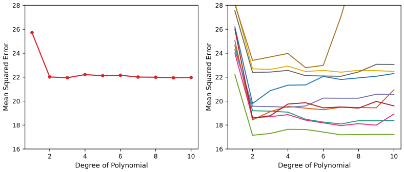
mpg on horsepower, against the degree. Left: one random split. Right: ten other random splits. Every split agrees that the straight line is worst, but the level of the curve moves by several units from split to split (at degree 2, from 17.1 to 23.4 over the eleven splits), and the curves do not agree on the best degree. One split puts a few extreme cars only in the validation half, where high-degree polynomials extrapolate badly. Splits are random halves from numpy seed 2021. Code: ch05_resampling_methods.py, fig_5_2. Reproduces James et al. (2021), Figure 5.2. Download: PDF · SVGp. 200 The approach has two weaknesses. (1) The estimate depends heavily on which observations land in which half: it is highly variable. (2) Only half of the data are used to fit, and a method fitted to fewer observations usually predicts worse, so the validation error tends to overestimate the test error of the method fitted to all \(n\) observations. How large is that second effect? For least squares it can be computed exactly.
Filling the gap 5.1: how much worse is a fit to fewer observations? p. 200, drawback 2
For least squares with an intercept, \(p\) Gaussian inputs and a correct linear model with noise variance \(\sigma^2\), the expected test error of a fit to \(m\) observations is
\[ \Err(m)=\sigma^2\Big(1+\frac1m+\Big(1+\frac1m\Big)\frac{p}{m-p-2}\Big),\qquad m>p+2, \]which decreases in \(m\). Validation with half the data estimates \(\Err(n/2)\), not \(\Err(n)\).
Derivation
Error at a new point. Write \(\tilde x=(1,x^\T)^\T\) and \(y_0=\tilde x_0^\T\bb+\varepsilon_0\) for a new observation, independent of the \(m\) training pairs. The prediction error is \(y_0-\tilde x_0^\T\hb=\varepsilon_0-\tilde x_0^\T(\hb-\bb)\), and given the training inputs \(\hb-\bb\) has mean zero and covariance \(\sigma^2(\bX^\T\bX)^{-1}\) (Section 3.1.2 of the book). The two terms are independent, so
\[ \E\big[(y_0-\tilde x_0^\T\hb)^2\given \bX,x_0\big]=\sigma^2\big(1+\tilde x_0^\T(\bX^\T\bX)^{-1}\tilde x_0\big). \]The intercept separates. Inverting \(\bX^\T\bX\) by blocks (or refitting with centred inputs, which does not change the fit) gives the identity \(\tilde x_0^\T(\bX^\T\bX)^{-1}\tilde x_0=\frac1m+(x_0-\bar x)^\T\bS^{-1}(x_0-\bar x)\), where \(\bS=\sum_{i=1}^m(x_i-\bar x)(x_i-\bar x)^\T\).
Average over Gaussian inputs. If the inputs are independent \(\N(\mu,\bSig)\), then \(\bS\) has a Wishart distribution with \(m-1\) degrees of freedom and scale \(\bSig\), it is independent of \(\bar x\), and \(\E\bS^{-1}=\bSig^{-1}/(m-p-2)\). Also \(x_0-\bar x\sim\N\big(0,(1+\frac1m)\bSig\big)\), independent of \(\bS\). Hence
\[ \E\big[(x_0-\bar x)^\T\bS^{-1}(x_0-\bar x)\big]=\tr\Big(\E\bS^{-1}\,\E\big[(x_0-\bar x)(x_0-\bar x)^\T\big]\Big)=\frac{(1+\frac1m)\tr(\bSig^{-1}\bSig)}{m-p-2}=\Big(1+\frac1m\Big)\frac{p}{m-p-2}. \]Adding the pieces gives the formula. ∎
What it says. With \(n=392\) and \(p=2\), \(\Err(196)=1.0156\,\sigma^2\) against \(\Err(392)=1.0077\,\sigma^2\): the half-size fit is less than 1% worse, so on data like Auto the validation estimate's problem is its variability, not its bias. (In the demonstration, 100 validation splits average 19.39 at degree 2 against 19.25 for LOOCV, 0.7% higher.) With \(n=50\) and \(p=10\) the picture changes: \(\Err(25)=1.84\,\sigma^2\) against \(\Err(50)=1.29\,\sigma^2\). Confirmed numerically by simulation (Filling the gap 5.3): over 2,000 data sets the validation estimates average 1.844 against the formula's 1.840.
5.1.2 Leave-One-Out Cross-Validation
Definition 5.2 (LOOCV) pp. 200–201, (5.1), Figure 5.3
For each \(i=1,\dots,n\), fit the method to the \(n-1\) observations other than \(i\), predict \(y_i\) by \(\hat y_i^{(-i)}\) and record \(\MSE_i=(y_i-\hat y_i^{(-i)})^2\). The leave-one-out cross-validation estimate is the average
\[ \CV_{(n)}=\frac1n\sum_{i=1}^n\MSE_i. \tag{5.1} \]p. 201 Each \(\MSE_i\) is a nearly unbiased but very noisy estimate of the test error (it rests on one observation); their average is much less noisy. Compared with a validation set, LOOCV fits on \(n-1\) observations instead of about \(n/2\), so it is far less biased upwards, and it involves no random split: run it twice and you get the same number. Its apparent cost is \(n\) fits. For least squares that cost disappears.
Result 5.1 (LOOCV from a single fit) p. 202, (5.2) and footnote 1
For least squares with any design matrix of full rank (simple, polynomial or multiple regression),
\[ \CV_{(n)}=\frac1n\sum_{i=1}^n\Big(\frac{y_i-\hat y_i}{1-h_i}\Big)^2, \tag{5.2} \]where \(\hat y_i\) and \(h_i\) are the fitted values and leverages of the fit to all \(n\) observations. When the model has an intercept, \(1/n\le h_i\le1\). The same identity holds, with \(h_i\) replaced by the diagonal element \(\bS_{ii}\) of the smoother matrix, for ridge regression and for smoothing splines.
Filling the gap 5.2: why (5.2) holds, and why the leverages lie in \([1/n,1]\) p. 202, "the following formula holds"
The book states (5.2) without proof. One short argument covers least squares, ridge regression and smoothing splines at once: deleting an observation is the same as replacing its response by its own leave-one-out prediction.
Derivation
Setting. Let the fit to responses \(\by\) be \(\hat\by=\bS\by\) for a fixed matrix \(\bS\) (\(\bS=\bH\) for least squares), and suppose the fit is the minimiser of a criterion of the form \(\sum_k(y_k-f(x_k))^2+J(f)\) over a class of functions \(f\) that does not depend on \(\by\) (\(J=0\) for least squares, \(J(f)=\lambda\sum_j\beta_j^2\) for ridge, \(J(f)=\lambda\int f''(t)^2\,dt\) for a smoothing spline).
Step 1: the leave-one-out fit is a full-data fit. Let \(f^{(-i)}\) minimise the criterion without the \(i\)th term, and build new responses \(\by^*\) equal to \(\by\) except \(y_i^*=f^{(-i)}(x_i)\). For every \(f\),
\[ \sum_{k}\big(y_k^*-f(x_k)\big)^2+J(f)\ \ge\ \sum_{k\ne i}\big(y_k-f(x_k)\big)^2+J(f)\ \ge\ \sum_{k\ne i}\big(y_k-f^{(-i)}(x_k)\big)^2+J(f^{(-i)}), \]and \(f=f^{(-i)}\) attains the right-hand side with equality, because its \(i\)th term is zero. So \(f^{(-i)}\) is the full-data fit for the responses \(\by^*\).
Step 2: solve for the prediction. Hence \(\hat y_i^{(-i)}=f^{(-i)}(x_i)=\sum_k\bS_{ik}y_k^*=\sum_{k\ne i}\bS_{ik}y_k+\bS_{ii}\hat y_i^{(-i)}\). Since \(\sum_{k\ne i}\bS_{ik}y_k=\hat y_i-\bS_{ii}y_i\),
\[ \hat y_i^{(-i)}=\frac{\hat y_i-\bS_{ii}y_i}{1-\bS_{ii}},\qquad y_i-\hat y_i^{(-i)}=\frac{y_i(1-\bS_{ii})-\hat y_i+\bS_{ii}y_i}{1-\bS_{ii}}=\frac{y_i-\hat y_i}{1-\bS_{ii}}. \]Squaring and averaging gives (5.2), with \(h_i=\bH_{ii}\) for least squares. The same algebra, written with the Sherman–Morrison formula for \((\bX^\T\bX-x_ix_i^\T)^{-1}\), is the textbook proof for least squares.
The leverages. \(\bH\) is symmetric and idempotent, so \(h_i=(\bH^2)_{ii}=\sum_kh_{ik}^2\ge h_i^2\), which gives \(h_i\le1\). With an intercept, the identity of Filling the gap 5.1 applied at \(x_0=x_i\) gives \(h_i=\frac1n+(x_i-\bar x)^\T\bS^{-1}(x_i-\bar x)\ge\frac1n\) (here \(\bS\) is the scatter matrix, which is positive definite). In simple regression this is the book's (3.37), \(h_i=\frac1n+(x_i-\bar x)^2/\sum_k(x_k-\bar x)^2\). A point far from the mean of the inputs has a large leverage, pulls the fit towards itself, and has its residual inflated the most by (5.2). Without an intercept the lower bound can fail. ∎
Confirmed numerically: on Auto the shortcut and 392 refits agree to twelve digits for every degree (24.2315 at degree 1); for smoothing splines, the shortcut with \(\bS_{ii}\) and \(n\) refits agree to nine digits (spline_loocv and spline_loocv_brute in the code). The largest leverage on Auto at degree 2 is 0.094, for the car with 230 horsepower (the average leverage is \(3/392=0.008\)).
Deeper: Statistical Learning: Theory and Methods, Result 7.13 (leave-one-out from one fit, and generalised cross-validation, which replaces each \(h_i\) by their average).
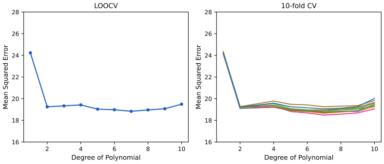
fig_5_4. Reproduces James et al. (2021), Figure 5.4. Download: PDF · SVGpp. 202–203 LOOCV applies to any method (logistic regression, discriminant analysis, the methods of later chapters); only the one-fit formula is special. For a general method it costs \(n\) fits.
5.1.3 k-Fold Cross-Validation
Definition 5.3 (k-fold cross-validation) p. 203, (5.3), Figure 5.5
Divide the observations at random into \(k\) groups (folds) of roughly equal size. For \(j=1,\dots,k\), fit on the other \(k-1\) folds and compute the mean squared error \(\MSE_j\) on fold \(j\). The estimate is
\[ \CV_{(k)}=\frac1k\sum_{j=1}^k\MSE_j. \tag{5.3} \]LOOCV is the case \(k=n\). The common choices are \(k=5\) and \(k=10\).
Algorithm 5.1 (choosing a flexibility by k-fold CV)
- Assign each observation a fold label in \(\{1,\dots,k\}\) by a random permutation of \(1,2,\dots,k,1,2,\dots\) (so fold sizes differ by at most one).
- For each candidate flexibility \(d\) (degree, \(K\), \(\lambda\)) and each fold \(j\): fit with flexibility \(d\) to the observations outside fold \(j\); record \(\MSE_j(d)\) on fold \(j\).
- Compute \(\CV_{(k)}(d)\) by (5.3), choose \(\hat d\) with the smallest value, and refit with \(\hat d\) on all \(n\) observations.
Every step that uses the responses, including any screening of predictors, must be repeated inside the loop; see the wrong and right way to cross-validate.
pp. 203–204 The obvious advantage over LOOCV is cost: 5 or 10 fits instead of \(n\), which matters for slow methods (the shortcut (5.2) is the exception). If the folds have unequal sizes, (5.3) and the average of all \(n\) held-out squared errors, \(\frac1n\sum_j n_j\MSE_j\), differ slightly; R's cv.glm() reports the second (Filling the gap 5.8). The right panel of Figure 5.4 shows that the randomness of the partition moves 10-fold CV only a little.
pp. 204–205 On real data the true test error is unknown, so the accuracy of CV can be judged only on simulated data. Figure 5.6 does that for smoothing splines (Chapter 7) on three simulated data sets of the kind used in Chapter 2.
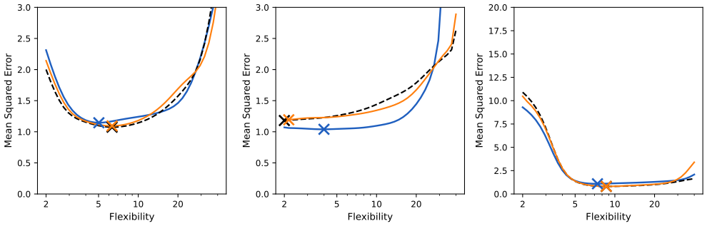
fig_5_6, SmoothingSpline. Reproduces James et al. (2021), Figure 5.6. Download: PDF · SVGp. 205 Two uses of CV should be kept apart. For model assessment the value of \(\CV(d)\) matters; for model selection only the location of its minimum does, and Figure 5.6 shows that the location can be right even when the level is off.
5.1.4 Bias-Variance Trade-Off for k-Fold Cross-Validation
pp. 205–206 Beyond cost, the choice of \(k\) trades bias against variance. Bias: each fit in k-fold CV uses about \((k-1)n/k\) observations, so CV estimates the error of a fit to that many points, which is a little larger than the error of a fit to all \(n\) (Filling the gap 5.1). The validation set (half the data) is the most biased, LOOCV (\(n-1\) points) the least. Variance: the book's argument is that LOOCV averages \(n\) fits trained on almost the same data, whose errors are therefore highly correlated, and the mean of highly correlated quantities has a high variance; k-fold CV averages fewer, less correlated fits. Its recommendation, \(k=5\) or \(k=10\), is a compromise found to work well in practice.
Filling the gap 5.3: the variance of a mean of correlated terms, and what a simulation shows pp. 205–206
The mean of \(m\) terms with common variance \(\sigma^2\) and common pairwise correlation \(\rho\) has variance \(\sigma^2\big(\rho+\frac{1-\rho}m\big)\): averaging removes only the uncorrelated part. That is the mechanism behind the book's argument. But the argument compares two things that differ in several ways at once, and for least squares the conclusion does not hold.
Derivation and simulation
The formula. \(\Var\big(\frac1m\sum_jZ_j\big)=\frac1{m^2}\big(\sum_j\Var Z_j+\sum_{j\ne l}\Cov(Z_j,Z_l)\big)=\frac1{m^2}\big(m\sigma^2+m(m-1)\rho\sigma^2\big)=\sigma^2\big(\rho+\frac{1-\rho}m\big)\). As \(m\to\infty\) it tends to \(\rho\sigma^2\), not to zero.
Why the comparison is not clear-cut. LOOCV averages \(n\) terms (each one squared error) with high correlation; \(\CV_{(k)}\) averages \(k\) terms (each a mean over \(n/k\) points) with lower correlation, and it also carries the randomness of the partition, which LOOCV does not have. Which effect wins depends on the method: for a stable method, such as least squares, small changes in the training set barely change the fit, and LOOCV does well.
Simulation (cv_study): \(n=50\), \(p=10\) standard Gaussian inputs, \(y=1+x^\T\bb+\varepsilon\) with \(\|\bb\|=1\) and \(\varepsilon\sim\N(0,1)\), least squares, 2,000 data sets, a new random partition for every estimate. \(\Err_\mathcal{T}\) is the true test error of the fit to all 50 points (exact, since the model is known): its average is 1.291, the formula of Filling the gap 5.1 gives 1.288.
| estimate | fits on | mean | \(\Err(m)\) formula | standard deviation | root mean squared error about \(\Err_\mathcal{T}\) |
|---|---|---|---|---|---|
| validation (half) | 25 | 1.844 | 1.840 | 0.781 | 0.967 |
| \(\CV_{(2)}\) | 25 | 1.848 | 1.840 | 0.627 | 0.848 |
| \(\CV_{(5)}\) | 40 | 1.387 | 1.391 | 0.359 | 0.392 |
| \(\CV_{(10)}\) | 45 | 1.329 | 1.332 | 0.324 | 0.351 |
| LOOCV | 49 | 1.294 | 1.296 | 0.298 | 0.326 |
Three lessons. (1) The bias is exactly as predicted: each estimate's mean matches the expected error of a fit to the number of points it actually trains on. (2) Here LOOCV has the smallest standard deviation, not the largest, so the book's claim that LOOCV has higher variance than k-fold CV is not a general fact; it holds for some procedures and fails for others (Burman 1989; Arlot and Celisse 2010). (3) No estimate tracks the error of the particular fit: the correlation between each estimate and \(\Err_\mathcal{T}\) is below 0.04 in every row. Cross-validation estimates the average error of the procedure over training sets, which is the point of Section 7.12 of the graduate course. ∎
Deeper: Statistical Learning: Theory and Methods, Section 7.10.1 (the learning curve and the choice of \(k\)) and Result 7.15 (in a correct Gaussian linear model, CV carries no information about the error of the fit at hand).
5.1.5 Cross-Validation on Classification Problems
Definition 5.4 (CV error rate for classification) p. 206, (5.4)
For a qualitative response the squared error is replaced by the indicator of a mistake, \(\mathrm{Err}_i=\I(y_i\ne\hat y_i^{(-i)})\), and
\[ \CV_{(n)}=\frac1n\sum_{i=1}^n\mathrm{Err}_i. \tag{5.4} \]The k-fold and validation-set error rates are defined in the same way.
pp. 206–208 The book fits logistic regressions with polynomial terms to the two-class data of Figure 2.13, for example the quadratic model
\[ \log\Big(\frac{p}{1-p}\Big)=\beta_0+\beta_1X_1+\beta_2X_1^2+\beta_3X_2+\beta_4X_2^2, \tag{5.5} \]and, in general, a degree-\(d\) model with the terms \(X_1,\dots,X_1^d,X_2,\dots,X_2^d\) (no products). Since the data are simulated, the true test error and the Bayes error are known.
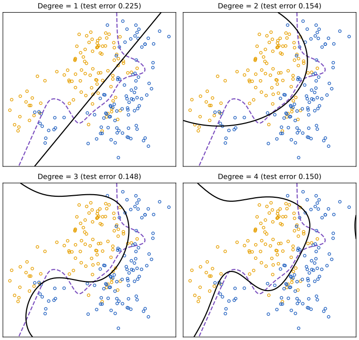
fig_5_7, logistic_fit. Reproduces James et al. (2021), Figure 5.7. Download: PDF · SVG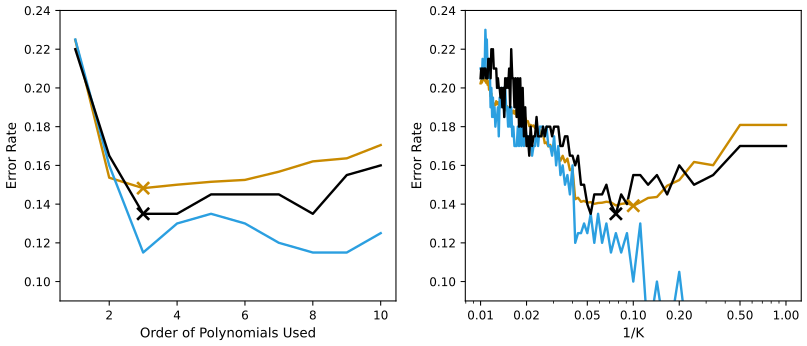
fig_5_8. Reproduces James et al. (2021), Figure 5.8. Download: PDF · SVGFilling the gap 5.4: why the training error rate need not fall as the degree grows p. 208, "doesn't quite decrease monotonically"
Explanation
The polynomial models are nested: the degree-\((d+1)\) model contains the degree-\(d\) model (set the two new coefficients to zero). Logistic regression maximises the likelihood, so the maximised log-likelihood of the bigger model is at least that of the smaller one, and the training deviance can only fall with \(d\). The misclassification rate is a different quantity: it counts points on the wrong side of the boundary \(\hat p=0.5\), which the fit does not optimise. A higher-degree fit can raise the likelihood by making confident points more confident while moving the boundary across a few borderline points, so the count of mistakes can go up. For least squares there is no such gap, because the training criterion and the reported training error are the same quantity (the RSS). ∎
For real data the Bayes boundary and the test error are unknown, and the 10-fold CV curve is the practical guide: in Figure 5.8 it underestimates the test error somewhat, but its minimum is close to the best degree and the best \(K\).
5.2 The Bootstrap
p. 209 The bootstrap measures the uncertainty of an estimate or of a learning method. For the coefficients of a linear regression this is not needed, since formulas exist; its value is that it works in the same way for estimates whose variability has no formula. The book's example is an investment problem. Returns \(X\) and \(Y\) of two assets are random; we invest a fraction \(\alpha\) in \(X\) and \(1-\alpha\) in \(Y\), and want the least risky mix, the one that minimises \(\Var(\alpha X+(1-\alpha)Y)\).
Result 5.2 (the minimum-variance allocation) p. 209, (5.6)–(5.7); Exercise 5.1
With \(\sigma_X^2=\Var(X)\), \(\sigma_Y^2=\Var(Y)\), \(\sigma_{XY}=\Cov(X,Y)\) and \(\Var(X-Y)=\sigma_X^2+\sigma_Y^2-2\sigma_{XY}>0\), the risk is minimised by
\[ \alpha=\frac{\sigma_Y^2-\sigma_{XY}}{\sigma_X^2+\sigma_Y^2-2\sigma_{XY}}, \tag{5.6} \]and the minimum risk is \((\sigma_X^2\sigma_Y^2-\sigma_{XY}^2)/\Var(X-Y)\). With past returns, the plug-in estimate is
\[ \hat\alpha=\frac{\hat\sigma_Y^2-\hat\sigma_{XY}}{\hat\sigma_X^2+\hat\sigma_Y^2-2\hat\sigma_{XY}}. \tag{5.7} \]Moreover \(\alpha\) is the slope of the population regression of \(-Y\) on \(X-Y\), and \(\hat\alpha\) is exactly the least-squares slope of \(-y_i\) on \(x_i-y_i\).
Filling the gap 5.5: deriving (5.6), and what the regression form buys p. 209, "one can show"; Exercise 5.1
Derivation
Calculus. By the rules for the variance of a linear combination,
\[ f(\alpha)=\Var(\alpha X+(1-\alpha)Y)=\alpha^2\sigma_X^2+(1-\alpha)^2\sigma_Y^2+2\alpha(1-\alpha)\sigma_{XY}. \]Then \(f'(\alpha)=2\alpha\sigma_X^2-2(1-\alpha)\sigma_Y^2+2(1-2\alpha)\sigma_{XY}\), and \(f'(\alpha)=0\) is \(\alpha(\sigma_X^2+\sigma_Y^2-2\sigma_{XY})=\sigma_Y^2-\sigma_{XY}\), which is (5.6). Since \(f''(\alpha)=2(\sigma_X^2+\sigma_Y^2-2\sigma_{XY})=2\Var(X-Y)>0\), the quadratic \(f\) is convex and this stationary point is its global minimum. (If \(\Var(X-Y)=0\) the two assets differ by a constant and every \(\alpha\) has the same risk.) Nothing forces \(\alpha\) into \([0,1]\): a value outside means selling one asset short.
Regression form. Write \(\alpha X+(1-\alpha)Y=Y+\alpha D\) with \(D=X-Y\), and \(W=-Y\). Then \(\Var(Y+\alpha D)=\Var(W-\alpha D)\), and the \(\alpha\) minimising \(\Var(W-\alpha D)\) is the regression slope \(\Cov(W,D)/\Var(D)=(\sigma_Y^2-\sigma_{XY})/\Var(X-Y)\), the same as (5.6). The minimum is the residual variance \(\Var(W)-\Cov(W,D)^2/\Var(D)=\sigma_Y^2-(\sigma_Y^2-\sigma_{XY})^2/\Var(X-Y)\), which simplifies to \((\sigma_X^2\sigma_Y^2-\sigma_{XY}^2)/\Var(X-Y)\). In the sample, (5.7) is \(\widehat{\Cov}(w,d)/\widehat{\Var}(d)\) with \(w_i=-y_i\), \(d_i=x_i-y_i\): the least-squares slope.
What it buys. If \((X,Y)\) is bivariate normal, then given the \(d_i\) the \(w_i\) follow a correct linear model with normal errors of variance \(\sigma_P^2\) (the minimum risk). So \(\hat\alpha\) is exactly unbiased, and its conditional variance is \(\sigma_P^2/\sum_i(d_i-\bar d)^2\). Since \(\sum_i(d_i-\bar d)^2/\Var(D)\) has a \(\chi^2_{n-1}\) distribution and \(\E[1/\chi^2_{n-1}]=1/(n-3)\),
\[ \SE(\hat\alpha)=\sqrt{\frac{\sigma_P^2}{(n-3)\Var(X-Y)}}. \]For the book's population (\(\sigma_X^2=1\), \(\sigma_Y^2=1.25\), \(\sigma_{XY}=0.5\)): \(\alpha=0.75/1.25=0.6\), \(\sigma_P^2=(1.25-0.25)/1.25=0.8\), and with \(n=100\), \(\SE(\hat\alpha)=\sqrt{0.8/(97\times1.25)}=0.0812\). The book's simulation gives a mean of 0.5996 and a standard deviation of 0.083; ours (Figure 5.10) 0.5987 and 0.0828. On the Portfolio data alone, the usual least-squares standard error of that slope is 0.0888, a formula answer to compare with the bootstrap's 0.09. ∎
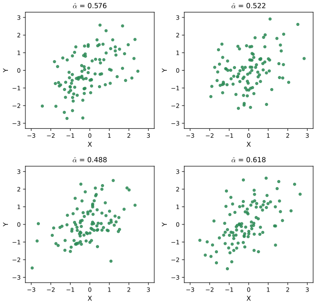
fig_5_9. Reproduces James et al. (2021), Figure 5.9. Download: PDF · SVGpp. 209–211 With access to the population, the accuracy of \(\hat\alpha\) is easy to find: draw 1,000 data sets, compute \(\hat\alpha_1,\dots,\hat\alpha_{1000}\), and take their standard deviation. With real data we have one sample, and the bootstrap imitates "drawing a new data set" by drawing from the sample.
Definition 5.5 (the nonparametric bootstrap and its standard error) pp. 211–212, (5.8), Figure 5.11
A bootstrap data set \(Z^{*}\) is a sample of \(n\) observations drawn with replacement from the original data set \(Z\) (whole rows: an observation brings its \(X\) and its \(Y\)). Repeating \(B\) times gives \(Z^{*1},\dots,Z^{*B}\) and estimates \(\hat\alpha^{*1},\dots,\hat\alpha^{*B}\), and the bootstrap standard error is their standard deviation,
\[ \SE_B(\hat\alpha)=\sqrt{\frac1{B-1}\sum_{r=1}^B\Big(\hat\alpha^{*r}-\frac1B\sum_{r'=1}^B\hat\alpha^{*r'}\Big)^2}. \tag{5.8} \]Algorithm 5.2 (the bootstrap standard error of any statistic)
- Write the statistic as a function of the data and a list of row numbers, \(s(Z,\text{idx})\), so that \(s(Z,1{:}n)\) is the estimate itself.
- For \(r=1,\dots,B\): draw idx as \(n\) integers uniform on \(1,\dots,n\), with replacement, and compute \(\hat\theta^{*r}=s(Z,\text{idx})\).
- Report \(\SE_B\) by (5.8). Also useful: the bootstrap bias \(\bar\theta^*-\hat\theta\) and the histogram of the \(\hat\theta^{*r}\).
This is what R's boot() and the Python function boot_se of the lab do (Section 5.3.4).
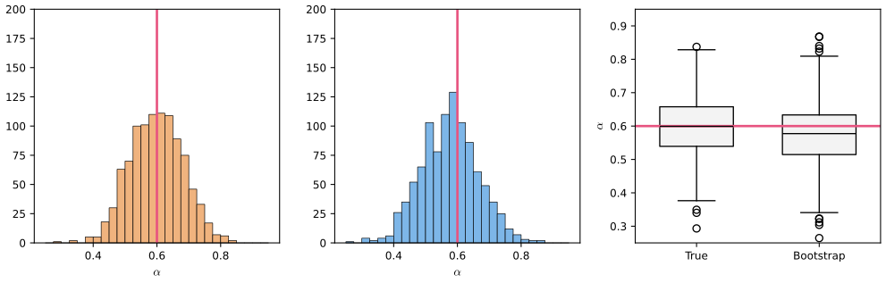
fig_5_10. Reproduces James et al. (2021), Figure 5.10. Download: PDF · SVGFilling the gap 5.6: what the bootstrap standard error estimates, and how large \(B\) must be pp. 210–212
Explanation
The plug-in principle. The sampling distribution of \(\hat\alpha\) depends on the unknown distribution \(F\) of \((X,Y)\): draw \(n\) pairs from \(F\), compute \(\hat\alpha\). The bootstrap replaces \(F\) by the empirical distribution \(\hat F_n\), which puts mass \(1/n\) on each observed pair; drawing \(n\) pairs from \(\hat F_n\) is exactly sampling the rows with replacement. So the ideal bootstrap standard error is \(\SE_{\hat F_n}(\hat\alpha^*)\), the standard deviation of \(\hat\alpha^*\) over all \(n^n\) equally likely resamples, and it estimates \(\SE_F(\hat\alpha)\) because \(\hat F_n\) is close to \(F\) for large \(n\). Formula (5.8) approximates the ideal value by \(B\) random resamples.
A case done exactly: the sample mean. If \(\hat\theta=\bar y\), then \(\bar y^*\) is a mean of \(n\) independent draws from \(\hat F_n\), whose variance is \(\hat\sigma^2=\frac1n\sum_i(y_i-\bar y)^2\). Hence \(\Var_*(\bar y^*)=\hat\sigma^2/n\): the ideal bootstrap standard error is \(\frac{s}{\sqrt n}\sqrt{\frac{n-1}n}\), the textbook formula times \(\sqrt{(n-1)/n}\). For Boston medv (Exercise 9) that is \(0.4089\times0.9990=0.4085\).
The Monte Carlo error of \(\SE_B\). For fixed data, \(\SE_B\) is itself random. If the \(\hat\alpha^{*r}\) are roughly normal, \(\SE_B^2\) behaves like a sample variance from \(B\) draws, with \(\Var(\SE_B^2)\approx2\SE^4/(B-1)\); the delta method then gives \(\mathrm{sd}(\SE_B)\approx\SE/\sqrt{2(B-1)}\). With \(B=1000\) that is about 2.2% of the standard error, i.e. \(\pm0.002\) for \(\hat\alpha\). This explains why the R lab reports 0.0897 and the Python lab 0.0912 for the same data: they use different random resamples. For a standard error, \(B\) of a few hundred to a thousand is enough; percentiles of the bootstrap distribution need more.
When it fails. The argument needs the statistic to depend smoothly on \(\hat F_n\). It works for means, variances, ratios such as \(\hat\alpha\), regression coefficients and medians; it is known to fail for extremes such as the sample maximum, whose bootstrap distribution has a point mass of \(1-(1-1/n)^n\approx0.632\) at the observed maximum (Result 5.3). ∎
p. 211 In Figure 5.11 the book draws a bootstrap sample of a data set with \(n=3\) observations that contains the third observation twice, the first once and the second not at all. How often is a given observation left out?
Result 5.3 (an observation's chance of being in a bootstrap sample) Exercise 5.2
In a bootstrap sample of size \(n\), the number of copies of observation \(j\) has a Binomial\((n,1/n)\) distribution, so
\[ \Pr(j\text{ is in the sample})=1-\Big(1-\frac1n\Big)^n, \]which decreases from 1 (\(n=1\)) to the limit \(1-e^{-1}=0.6321\). It is 0.7037 for \(n=3\), 0.6723 for \(n=5\), 0.6340 for \(n=100\) and 0.6321 for \(n=10{,}000\). The number \(D\) of distinct observations in the sample has mean \(n\big(1-(1-1/n)^n\big)\) and variance \(n q_1+n(n-1)q_2-n^2q_1^2\), with \(q_1=(1-1/n)^n\) and \(q_2=(1-2/n)^n\).
Filling the gap 5.7: proofs for Result 5.3 Exercise 5.2
Derivation
The probability. The \(n\) draws are independent and each picks observation \(j\) with probability \(1/n\). So each draw misses \(j\) with probability \(1-1/n\), all \(n\) draws miss it with probability \((1-1/n)^n\), and the number of copies is Binomial\((n,1/n)\).
The limit. \(\log(1-1/n)^n=n\log(1-1/n)=-1-\frac1{2n}-\frac1{3n^2}-\cdots\to-1\), so \((1-1/n)^n\to e^{-1}=0.3679\). The same expansion shows the copies of one observation tend to a Poisson(1) law: \(\binom nk n^{-k}(1-1/n)^{n-k}\to e^{-1}/k!\).
Monotonicity. Let \(g(x)=x\log(1-1/x)\) for \(x>1\). Then \(g'(x)=\log(1-t)+\frac{t}{1-t}\) with \(t=1/x\in(0,1)\), and since \(-\log(1-t)=\sum_{k\ge1}t^k/k<\sum_{k\ge1}t^k=\frac t{1-t}\), \(g'(x)>0\). So \((1-1/n)^n\) increases with \(n\) and the inclusion probability decreases towards 0.632: larger samples leave out a larger fraction, but never more than 36.8%.
The number of distinct observations. Let \(E=\sum_j\I(j\text{ not drawn})\), so \(D=n-E\). \(\E E=nq_1\). Two given observations are both missed with probability \((1-2/n)^n=q_2\), so \(\E E^2=nq_1+n(n-1)q_2\) and \(\Var D=\Var E=nq_1+n(n-1)q_2-n^2q_1^2\). For \(n=100\), \(D\) has mean 63.40 and standard deviation 3.12; for \(n=1000\), 632.3 and 9.86. For \(n=3\) the exact distribution is \(\Pr(D=1,2,3)=3/27,\,18/27,\,6/27\): two distinct observations, as in Figure 5.11, is the most likely case. ∎
Confirmed numerically: the exact distribution of \(D\) (computed one draw at a time, distinct_count_pmf) has the mean and variance above for every \(n\) up to 1000.
Deeper: the 0.632 reappears in error estimation: a bootstrap fit sees only about 63% of the distinct observations, which motivates the .632 estimator, Statistical Learning: Theory and Methods, Section 7.11 (Result 7.14, Filling the gap 7.9). The parametric bootstrap and its link to maximum likelihood are in Section 8.2 (Result 8.1).
5.3 Lab: Cross-Validation and the Bootstrap
R edition pp. 212–219; Python edition pp. 215–224 The lab estimates the test error of polynomial regressions on Auto by the three cross-validation methods, then uses the bootstrap for \(\hat\alpha\) on Portfolio and for the regression coefficients on Auto. Each step is shown in R (left) and Python (right). The R code uses base R, the ISLR2 data and the boot package (cv.glm(), boot()), with the R lab's seeds; the Python code uses numpy, pandas, statsmodels and scikit-learn, with the Python lab's seeds. Both are my own code, written to answer the book's questions; they are excerpts of ch05_lab.R and ch05_lab.py, which run as they are. The two editions number the lab differently (the Python edition's 5.3.2 covers both LOOCV and k-fold, and its 5.3.3 is the bootstrap); the headings below follow the R edition.
Where R and Python differ, and why
- Deterministic quantities agree to every printed digit: LOOCV for every degree, the coefficients and formula standard errors of the linear and quadratic fits, the robust (sandwich) standard errors, \(\hat\alpha=0.5758\), and the LOOCV error of Exercise 7.
- Random splits differ. R's
sample()and numpy's generator are different random number generators, so the validation halves, the folds and the bootstrap resamples differ, and so do those numbers (23.27 against 23.62 for the first validation split). Each column reproduces its own edition's printed output. Fed the same split, the two languages give the same number: R's splitset.seed(1); sample(392, 196)used in Python gives R's 23.27, 18.72, 18.79. - k-fold CV is not computed in quite the same way. R's
cv.glm()draws new folds at every call (so each degree gets its own partition), its folds have random sizes (between 37 and 40 cars here) and it averages the fold MSEs weighted by fold size. The Python code uses oneKFoldpartition for all degrees, with folds of 39 or 40, and the plain average (5.3). - The bootstrap standard error. R's
boot()and the Pythonboot_sehere both use the divisor \(B-1\) of (5.8). The Python edition's own function divides by \(B\); hence its 0.8488 where the code here prints 0.8492 for the same resamples (a factor \(\sqrt{1000/999}\)). - Orthogonal polynomials. R's
poly()builds orthogonal polynomials; the Python classPolyimplements the same three-term recurrence (fitted on the training data, then evaluated anywhere), so fits and predictions agree, and stay accurate up to degree 10, where raw powers of horsepower (up to \(230^{10}\)) would not.
Setting up
R ch05_lab.R
suppressPackageStartupMessages({
  library(ISLR2)   # the data sets: Auto, Portfolio, Default, Weekly, Boston
  library(boot)    # cv.glm() and boot()
})
options(digits = 5)
Python ch05_lab.py
import numpy as np
import pandas as pd
import statsmodels.api as sm
from scipy import stats
from sklearn.model_selection import KFold, ShuffleSplit, train_test_split

from common import isl_data

...

Auto = isl_data("Auto", na_values="?").dropna().reset_index(drop=True)   # 392 cars
Portfolio = isl_data("Portfolio")                                        # 100 pairs of returns
H, Y = Auto["horsepower"].to_numpy(float), Auto["mpg"].to_numpy(float)


# -- orthogonal polynomials, as R's poly()
class Poly:
    """Orthogonal polynomials of one variable. fit() learns the three-term recurrence on the
    training values (as R's poly() does); transform() evaluates the basis at any values. The
    columns span the same space as x, x^2, ..., x^d, so every fit and prediction is the
    ordinary polynomial one, but the least-squares problem stays well conditioned."""

    def __init__(self, degree):
        self.degree = degree

    def fit(self, x):
        x = np.asarray(x, float)
        d = self.degree
        self.alpha, self.norm2 = np.zeros(d), np.zeros(d + 2)
        self.norm2[0], self.norm2[1] = 1.0, len(x)
        p_old, p = np.zeros_like(x), np.ones_like(x)
        for k in range(d):
            self.alpha[k] = np.sum(x * p ** 2) / np.sum(p ** 2)
            p_old, p = p, (x - self.alpha[k]) * p - self.norm2[k + 1] / self.norm2[k] * p_old
            self.norm2[k + 2] = np.sum(p ** 2)
        return self

    def transform(self, x):
        x = np.asarray(x, float)
        Z = [np.ones_like(x), x - self.alpha[0]]
        for k in range(1, self.degree):
            Z.append((x - self.alpha[k]) * Z[k] - self.norm2[k + 1] / self.norm2[k] * Z[k - 1])
        Z = np.column_stack(Z[1:self.degree + 1]) / np.sqrt(self.norm2[2:])
        return np.column_stack([np.ones_like(x), Z])          # intercept first


def lstsq(X, y):
    return np.linalg.lstsq(X, y, rcond=None)[0]
5.3.1 The Validation Set Approach
Half of the 392 cars (196) train linear, quadratic and cubic fits, which are scored on the other half; then the same is done with a second random split.
R ch05_lab.R
# Fit a polynomial in horsepower on a random half of the 392 cars and
# score it by the mean squared error on the other half.
val_mse <- function(degree, train) {
  fit <- lm(mpg ~ poly(horsepower, degree), data = Auto, subset = train)
  mean((Auto$mpg - predict(fit, Auto))[-train]^2)
}
set.seed(1)
train <- sample(392, 196)
val_seed1 <- sapply(1:3, val_mse, train = train)
val_seed1                                   # 23.27 18.72 18.79

set.seed(2)                                 # a different split, different estimates
train <- sample(392, 196)
val_seed2 <- sapply(1:3, val_mse, train = train)
val_seed2                                   # 25.73 20.43 20.39
Python ch05_lab.py
# Fit a polynomial in horsepower on a random half of the cars and score it on the other half.
def val_mse(degree, train, valid):
    P = Poly(degree).fit(train["horsepower"])
    beta = lstsq(P.transform(train["horsepower"]), train["mpg"])
    pred = P.transform(valid["horsepower"]) @ beta
    return np.mean((valid["mpg"] - pred) ** 2)


Auto_train, Auto_valid = train_test_split(Auto, test_size=196, random_state=0)
val_seed0 = [val_mse(d, Auto_train, Auto_valid) for d in (1, 2, 3)]
show("validation, random_state=0:", np.round(val_seed0, 2))      # 23.62 18.76 18.80

Auto_train, Auto_valid = train_test_split(Auto, test_size=196, random_state=3)
val_seed3 = [val_mse(d, Auto_train, Auto_valid) for d in (1, 2, 3)]
show("validation, random_state=3:", np.round(val_seed3, 2)) # 20.76 16.95 16.97| validation MSE | linear | quadratic | cubic |
|---|---|---|---|
R, set.seed(1) | 23.27 | 18.72 | 18.79 |
R, set.seed(2) | 25.73 | 20.43 | 20.39 |
Python, random_state=0 | 23.62 | 18.76 | 18.80 |
Python, random_state=3 | 20.76 | 16.95 | 16.97 |
All four rows are the numbers printed in the two editions. Every split says the quadratic beats the line and the cubic adds nothing; the levels differ by several units, which is Figure 5.2's point.
5.3.2 Leave-One-Out Cross-Validation
R computes LOOCV with cv.glm(), which refits a glm() (without a family it is least squares) \(n\) times; the Python code does the \(n\) refits in a loop. Both then use the one-fit shortcut (5.2), with the leverages from hatvalues() in R and from a QR decomposition in Python.
R ch05_lab.R
# glm() without a family is least squares, and cv.glm() refits it n times.
glm_fit <- glm(mpg ~ horsepower, data = Auto)
coef(glm_fit)                               # 39.936 -0.158, as lm()
cv_glm <- cv.glm(Auto, glm_fit)
cv_glm$delta                                # 24.23 24.23

# The shortcut (5.2): one least-squares fit, each residual divided by 1 - h_i.
loocv_shortcut <- function(fit) mean((residuals(fit) / (1 - hatvalues(fit)))^2)
loocv_shortcut(lm(mpg ~ horsepower, data = Auto))   # 24.23 again

loocv <- sapply(1:10, function(d) {
  cv.glm(Auto, glm(mpg ~ poly(horsepower, d), data = Auto))$delta[1]
})
loocv_fast <- sapply(1:10, function(d) {
  loocv_shortcut(lm(mpg ~ poly(horsepower, d), data = Auto))
})
round(loocv, 2)                              # 24.23 19.25 19.33 19.42 19.03 18.98 18.83 18.96 19.07 19.49
all.equal(loocv, loocv_fast)                 # TRUE: n refits and one fit agree
Python ch05_lab.py
# By definition (5.1): leave each car out in turn, refit, predict it.
def loocv_brute(X, y):
    n = len(y)
    err = np.empty(n)
    for i in range(n):
        keep = np.arange(n) != i
        err[i] = (y[i] - X[i] @ lstsq(X[keep], y[keep])) ** 2
    return err.mean()


# By the shortcut (5.2): one fit; the leverages h_i are the squared row norms of Q in X = QR.
def loocv_shortcut(X, y):
    Q, _ = np.linalg.qr(X)
    h = np.sum(Q ** 2, axis=1)
    resid = y - Q @ (Q.T @ y)
    return np.mean((resid / (1 - h)) ** 2)


X1 = np.column_stack([np.ones_like(H), H])
show("LOOCV, 392 refits:", loocv_brute(X1, Y))                  # 24.2315
show("LOOCV, shortcut (5.2):", loocv_shortcut(X1, Y))           # the same
loocv = np.array([loocv_shortcut(Poly(d).fit(H).transform(H), Y) for d in range(1, 11)])
show("LOOCV, degrees 1-10:", np.round(loocv, 4))| degree | 1 | 2 | 3 | 4 | 5 | 6 | 7 | 8 | 9 | 10 |
|---|---|---|---|---|---|---|---|---|---|---|
| LOOCV (R and Python) | 24.23 | 19.25 | 19.33 | 19.42 | 19.03 | 18.98 | 18.83 | 18.96 | 19.07 | 19.49 |
The two languages agree to all digits (24.2315 at degree 1), and the refits and the shortcut agree too. The Python edition computes only degrees 1 to 5, with raw powers of horsepower; with orthogonal polynomials degrees 6–10 are no problem.
5.3.3 k-Fold Cross-Validation
Ten folds; in R a new partition for each degree (seed 17), in Python one partition for all degrees (random_state=0). The Python part also runs the validation set approach as a one-split ShuffleSplit, and ten such splits.
R ch05_lab.R
# cv.glm() draws new folds at every call, so each degree gets its own split.
set.seed(17)
cv10 <- matrix(NA, 10, 2, dimnames = list(1:10, c("CV", "adjusted")))
for (d in 1:10) {
  cv10[d, ] <- cv.glm(Auto, glm(mpg ~ poly(horsepower, d), data = Auto), K = 10)$delta
}
round(cv10[, "CV"], 2)                       # 24.27 19.27 19.35 19.29 19.03 18.90 19.12 19.15 18.87 20.96
round(cv10[, "adjusted"], 2)                 # the bias-corrected second number of delta
Python ch05_lab.py
# The same ten folds for every degree; CV(10) is the average of the ten fold MSEs (5.3).
def kfold_cv(degree, splitter):
    fold_mse = []
    for tr, te in splitter.split(H):
        P = Poly(degree).fit(H[tr])
        beta = lstsq(P.transform(H[tr]), Y[tr])
        fold_mse.append(np.mean((Y[te] - P.transform(H[te]) @ beta) ** 2))
    return np.mean(fold_mse), np.array(fold_mse)


folds = KFold(n_splits=10, shuffle=True, random_state=0)
cv10 = np.array([kfold_cv(d, folds)[0] for d in range(1, 11)])
show("10-fold CV, degrees 1-10:", np.round(cv10, 4))           # 24.2077 19.1853 19.2763 19.4785 19.1372 ...

# The validation set approach is a one-split "cross-validation": ShuffleSplit.
one_split = ShuffleSplit(n_splits=1, test_size=196, random_state=0)
show("validation via ShuffleSplit:", kfold_cv(1, one_split)[0])  # 23.6166
ten_splits = ShuffleSplit(n_splits=10, test_size=196, random_state=0)
val10 = kfold_cv(1, ten_splits)[1]
show("ten validation splits, mean and sd:", (round(val10.mean(), 4), round(val10.std(), 4))) # 23.8022 1.4218| degree | 1 | 2 | 3 | 4 | 5 | 6 | 7 | 8 | 9 | 10 |
|---|---|---|---|---|---|---|---|---|---|---|
R, cv.glm(K = 10) | 24.27 | 19.27 | 19.35 | 19.29 | 19.03 | 18.90 | 19.12 | 19.15 | 18.87 | 20.96 |
| R, adjusted (second number) | 24.25 | 19.25 | 19.33 | 19.27 | 19.00 | 18.86 | 19.06 | 19.09 | 18.82 | 20.75 |
Python, KFold(10) | 24.21 | 19.19 | 19.28 | 19.48 | 19.14 | 19.05 | 18.82 | 18.90 | 19.08 | 19.89 |
The R row is the R edition's output; the first five Python numbers (24.2077, 19.1853, 19.2763, 19.4785, 19.1372) are the Python edition's. The single ShuffleSplit gives 23.6166, the first validation split again, and ten splits give a mean of 23.80 with a standard deviation of 1.42. As the Python edition remarks, that standard deviation measures how much the estimate depends on the split; it is not a standard error of the test error, because the ten training sets overlap.
Filling the gap 5.8: the two numbers returned by cv.glm() R edition p. 216, "a bias-corrected version"
Explanation
Let \(n_j\) be the size of fold \(j\), \(\hat f^{(-j)}\) the fit without fold \(j\), \(\hat f\) the fit to all the data, and \(L(\cdot)\) the mean squared error over a set of points. The first number is \(\CV=\sum_j\frac{n_j}n\,L_j\big(\hat f^{(-j)}\big)\), the held-out error weighted by fold size, which equals (5.3) only when the folds have equal sizes. The second is
\[ \CV_{\text{adj}}=\CV+L_{\text{all}}\big(\hat f\big)-\sum_j\frac{n_j}n\,L_{\text{all}}\big(\hat f^{(-j)}\big), \]where \(L_{\text{all}}\) scores a fit on all \(n\) observations. The reasoning (Davison and Hinkley 1997, Section 6.4): \(\CV\) estimates the error of fits trained on about \((k-1)n/k\) points, which is too pessimistic for the fit to all \(n\) (Filling the gap 5.1); the difference between the apparent error of the full fit and the average apparent error of the fold fits, both measured on the whole data set, estimates how much better a fit to all \(n\) points does, and it is subtracted. The correction is small when \(k\) is large: here it lowers the estimates by 0.02 to 0.2. Confirmed numerically in R: recomputing both formulas by hand from the folds of set.seed(17) reproduces cv.glm()'s 19.2364 and 19.2233 for the quadratic. ∎
5.3.4 The Bootstrap
Estimating the accuracy of a statistic of interest. The statistic is written as a function of the data and a vector of row numbers; the bootstrap then calls it with resampled row numbers. R's boot() does the resampling; in Python a ten-line function does it.
R ch05_lab.R
# alpha_fn() returns the estimate (5.7) of the minimum-variance allocation,
# computed from the rows of the data listed in index.
alpha_fn <- function(data, index) {
  x <- data$X[index]
  y <- data$Y[index]
  (var(y) - cov(x, y)) / (var(x) + var(y) - 2 * cov(x, y))
}
alpha_fn(Portfolio, 1:100)                   # 0.576 from all 100 pairs

set.seed(7)
alpha_fn(Portfolio, sample(100, 100, replace = TRUE))   # 0.539: one bootstrap replicate

boot_alpha <- boot(Portfolio, alpha_fn, R = 1000)
boot_alpha                                   # original 0.5758, std. error 0.0897
sd(boot_alpha$t[, 1])                        # the same number, by (5.8)
Python ch05_lab.py
def alpha_func(D, idx):
    """The estimate (5.7) of the minimum-variance allocation from the rows idx of D."""
    c = np.cov(D[["X", "Y"]].loc[idx], rowvar=False)
    return (c[1, 1] - c[0, 1]) / (c[0, 0] + c[1, 1] - 2 * c[0, 1])


show("alpha-hat from all 100 pairs:", alpha_func(Portfolio, range(100)))     # 0.5758
rng = np.random.default_rng(0)
show("one bootstrap replicate:", alpha_func(Portfolio, rng.choice(100, 100, replace=True)))   # 0.6074


def boot_se(func, D, B=1000, seed=0):
    """Bootstrap standard error (5.8) of func(D, idx): B resamples of the rows of D,
    drawn with replacement; returns the standard error and the B replicates."""
    rng = np.random.default_rng(seed)
    reps = np.array([func(D, rng.choice(D.index, len(D), replace=True)) for _ in range(B)])
    return reps.std(axis=0, ddof=1), reps


alpha_se, alpha_reps = boot_se(alpha_func, Portfolio, B=1000, seed=0)
show("bootstrap SE of alpha-hat:", alpha_se) # 0.0912| \(\hat\alpha\) | one resample | bootstrap SE, \(B=1000\) | |
|---|---|---|---|
| R (seed 7) | 0.5758 | 0.539 | 0.0897 |
| Python (seed 0) | 0.5758 | 0.6074 | 0.0912 |
The two standard errors differ by Monte Carlo noise of about \(\pm0.002\) (Filling the gap 5.6). Both are close to the least-squares standard error 0.0888 of Filling the gap 5.5 and to the true 0.081.
Estimating the accuracy of a linear regression model. Now the statistic is the pair \((\hat\beta_0,\hat\beta_1)\) of the regression of mpg on horsepower, and the bootstrap standard errors are compared with the formula ones of Section 3.1.2 and with robust (sandwich) standard errors.
R ch05_lab.R
boot_fn <- function(data, index) {
  coef(lm(mpg ~ horsepower, data = data, subset = index))
}
boot_fn(Auto, 1:392)                         # 39.936 -0.158

set.seed(1)
boot_fn(Auto, sample(392, 392, replace = TRUE))   # 40.341 -0.164
boot_fn(Auto, sample(392, 392, replace = TRUE))   # 40.119 -0.158
boot_lin <- boot(Auto, boot_fn, 1000)
se_boot_lin <- apply(boot_lin$t, 2, sd)
se_boot_lin                                  # 0.8413 0.0073

lin_fit <- lm(mpg ~ horsepower, data = Auto)
se_formula_lin <- summary(lin_fit)$coef[, "Std. Error"]
se_formula_lin                               # 0.7175 0.0064: smaller than the bootstrap

# The heteroscedasticity-robust (sandwich) standard errors, by hand:
# (X'X)^{-1} X' diag(e^2) X (X'X)^{-1}. They agree with the bootstrap, not with the formula.
sandwich_se <- function(fit) {
  X <- model.matrix(fit)
  e <- residuals(fit)
  bread <- solve(crossprod(X))
  sqrt(diag(bread %*% crossprod(X * e) %*% bread))
}
se_sandwich_lin <- sandwich_se(lin_fit)
se_sandwich_lin                              # 0.8536 0.0074

boot_fn2 <- function(data, index) {
  coef(lm(mpg ~ horsepower + I(horsepower^2), data = data, subset = index))
}
set.seed(1)
boot_quad <- boot(Auto, boot_fn2, 1000)
se_boot_quad <- apply(boot_quad$t, 2, sd)
se_boot_quad                                 # 2.0300 0.0324 0.0001
quad_fit <- lm(mpg ~ horsepower + I(horsepower^2), data = Auto)
se_formula_quad <- summary(quad_fit)$coef[, "Std. Error"]
se_formula_quad                              # 1.8004 0.0311 0.0001: now close
se_sandwich_quad <- sandwich_se(quad_fit)
se_sandwich_quad
Python ch05_lab.py
def boot_ols(degree, D, idx):
    """Least-squares coefficients of mpg on raw powers of horsepower, from the rows idx."""
    D_ = D.loc[idx]
    X = np.vander(D_["horsepower"].to_numpy(float), degree + 1, increasing=True)
    return lstsq(X, D_["mpg"].to_numpy(float))


def hp_func(D, idx):
    return boot_ols(1, D, idx)


def quad_func(D, idx):
    return boot_ols(2, D, idx)


rng = np.random.default_rng(0)
print(np.array([hp_func(Auto, rng.choice(392, 392, replace=True)) for _ in range(10)]))
se_boot_lin, _ = boot_se(hp_func, Auto, B=1000, seed=10)
show("bootstrap SEs, linear:", se_boot_lin)                     # 0.8488 0.0074

lin_fit = sm.OLS(Y, sm.add_constant(H)).fit()
se_formula_lin = lin_fit.bse
show("formula SEs, linear:", se_formula_lin)                    # 0.7175 0.0064: smaller


def sandwich_se(X, resid):
    """Heteroscedasticity-robust standard errors (X'X)^{-1} X' diag(e^2) X (X'X)^{-1}."""
    bread = np.linalg.inv(X.T @ X)
    meat = (X * resid[:, None] ** 2).T @ X
    return np.sqrt(np.diag(bread @ meat @ bread))


se_sandwich_lin = sandwich_se(lin_fit.model.exog, lin_fit.resid)
show("sandwich SEs, linear:", se_sandwich_lin)                  # 0.8536 0.0074: as the bootstrap

se_boot_quad, _ = boot_se(quad_func, Auto, B=1000, seed=0)
show("bootstrap SEs, quadratic:", se_boot_quad)                 # 2.0679 0.0330 0.0001
Xq = np.column_stack([np.ones_like(H), H, H ** 2])
quad_fit = sm.OLS(Y, Xq).fit()
se_formula_quad = quad_fit.bse
show("formula SEs, quadratic:", se_formula_quad)                # 1.8004 0.0311 0.0001: now close
se_sandwich_quad = sandwich_se(Xq, quad_fit.resid)| standard error | \(\hat\beta_0\) (linear) | \(\hat\beta_1\) (linear) | \(\hat\beta_0\) (quadratic) | \(\hat\beta_1\) (quadratic) | \(\hat\beta_2\) (quadratic) |
|---|---|---|---|---|---|
| formula \(\hat\sigma^2(\bX^\T\bX)^{-1}\) (R and Python) | 0.7175 | 0.00645 | 1.8004 | 0.0311 | 0.000122 |
bootstrap, R (set.seed(1)) | 0.8413 | 0.00734 | 2.0300 | 0.0324 | 0.000117 |
| bootstrap, Python (seeds 10 and 0) | 0.8492 | 0.00736 | 2.0689 | 0.0330 | 0.000120 |
| sandwich (R and Python) | 0.8536 | 0.00737 | 2.0742 | 0.0330 | 0.000119 |
The coefficients are 39.936 and \(-0.158\) (linear) and 56.900, \(-0.4662\), 0.00123 (quadratic) in both languages. The book explains why the bootstrap and the formula disagree for the straight line: the formula estimates \(\sigma^2\) from residuals that are inflated by the curvature the line misses, and it treats the \(x_i\) as fixed. The table adds a sharper statement: the bootstrap agrees with the sandwich standard errors, which are valid without a correct mean or a constant variance.
Filling the gap 5.9: resampling pairs approximates the sandwich formula R edition p. 218; Python edition p. 223
Derivation
A bootstrap sample of the rows is the same as giving row \(i\) a weight \(W_i\), the number of times it is drawn, with \((W_1,\dots,W_n)\) multinomial: \(\E W_i=1\), \(\Var W_i=1-\frac1n\), \(\Cov(W_i,W_k)=-\frac1n\). The bootstrap fit is the weighted least-squares fit \(\hb^*=\big(\sum_iW_ix_ix_i^\T\big)^{-1}\sum_iW_ix_iy_i\). Write \(y_i=x_i^\T\hb+e_i\) with the residuals \(e_i\) of the full fit; then
\[ \hb^*-\hb=\Big(\sum_iW_ix_ix_i^\T\Big)^{-1}\sum_iW_ix_ie_i=\Big(\sum_iW_ix_ix_i^\T\Big)^{-1}\sum_i(W_i-1)x_ie_i, \]because \(\sum_ix_ie_i=\mathbf0\) (the normal equations). For large \(n\), \(\sum_iW_ix_ix_i^\T\approx\bX^\T\bX\), so \(\Var_*(\hb^*)\approx(\bX^\T\bX)^{-1}\bA(\bX^\T\bX)^{-1}\) with
\[ \bA=\Var_*\Big(\sum_i(W_i-1)x_ie_i\Big)=\Big(1-\frac1n\Big)\sum_ie_i^2x_ix_i^\T-\frac1n\sum_{i\ne k}e_ie_kx_ix_k^\T=\sum_ie_i^2x_ix_i^\T, \]since \(\sum_{i\ne k}e_ie_kx_ix_k^\T=\big(\sum_ie_ix_i\big)\big(\sum_ke_kx_k\big)^\T-\sum_ie_i^2x_ix_i^\T=-\sum_ie_i^2x_ix_i^\T\). So the pairs bootstrap approximates the sandwich (heteroscedasticity-consistent, "HC0") covariance \((\bX^\T\bX)^{-1}\big(\sum_ie_i^2x_ix_i^\T\big)(\bX^\T\bX)^{-1}\) of White (1980). If the errors had constant variance and the model were right, \(\sum_ie_i^2x_ix_i^\T\approx\hat\sigma^2\bX^\T\bX\) and the sandwich would collapse to the formula \(\hat\sigma^2(\bX^\T\bX)^{-1}\). ∎
What the numbers say. For the straight line, the sandwich (0.854, 0.00737) and the bootstrap (0.841 and 0.849; 0.0073 and 0.0074) agree, and both exceed the formula (0.717, 0.00645) by 14 to 19%. For the quadratic the book says the agreement with the formula is "better", which is true for the slope terms, but the intercept's formula standard error (1.80) is still about 12% below the bootstrap and the sandwich (2.03 to 2.07): the spread of mpg around the quadratic is not constant across horsepower, so the constant-variance formula remains optimistic.
Notes on the book
Points where the text or the code of one of the editions disagrees with a computation, with the evidence. None changes the chapter's message.
1. Python edition, Exercise 2(h): the simulation draws one number, not a bootstrap sample Python edition p. 225
The printed loop is store[i] = np.sum(rng.choice(100, replace=True) == 4) > 0. Without a size argument, rng.choice(100, replace=True) returns a single integer, so the loop estimates the probability that one draw equals 4, about 0.01 (our run of the printed code: 0.0089), instead of the intended 0.634. The fix is rng.choice(100, 100, replace=True), which gives 0.6362 (Exercise 5.2). The same paragraph says the loop checks the "fifth observation", while the exercise says \(j=4\); in Python's 0-based numbering the value 4 is indeed the fifth row, so the two editions follow different observations (harmless, but confusing).
2. Python edition lab: the bootstrap function divides by \(B\), not \(B-1\) Python edition p. 221, In[18]
The function boot_SE of the Python lab returns \(\sqrt{\overline{\theta^{*2}}-\bar\theta^{*2}}\), the standard deviation with divisor \(B\), whereas (5.8), and R's boot(), use \(B-1\). The effect is a factor \(\sqrt{(B-1)/B}=0.9995\) for \(B=1000\): with the same resamples, 0.8488 (printed) against 0.8492 by (5.8), and 2.0678 against 2.0689. Negligible, but the code does not compute the formula it cites.
3. Section 5.1.4: "LOOCV has higher variance than does k-fold CV" is not a general fact p. 205
For least squares on simulated Gaussian data (\(n=50\), \(p=10\), 2,000 data sets; Filling the gap 5.3) the standard deviations are 0.298 for LOOCV, 0.324 for \(\CV_{(10)}\), 0.359 for \(\CV_{(5)}\) and 0.627 for \(\CV_{(2)}\): LOOCV is the least variable. The correlation argument in the book is one of several competing effects; whether LOOCV is more variable depends on the stability of the method (Burman 1989; Arlot and Celisse 2010). The practical advice (\(k=5\) or 10) is still sound, mostly on grounds of cost.
4. Smaller points
- p. 202: "The leverage lies between \(1/n\) and 1" holds for models with an intercept (Filling the gap 5.2); without one, leverages can be smaller than \(1/n\).
- R edition p. 215, and the Python lab: (5.3) averages the fold MSEs with equal weights, but
cv.glm()weights them by fold size and its folds have unequal, random sizes (37 to 40 cars forset.seed(17)); so the numbers in the R lab are not exactly (5.3). The difference is in the third decimal (Filling the gap 5.8). - Python edition, Exercise 7: "In Sections 5.1.2 and 5.1.3, we saw that the
cross_validate()function can be used..." The function appears in the lab, Section 5.3.2; the R edition's sentence correctly points to Sections 5.3.2 and 5.3.3. - Python edition, Exercise 8(c): "you may find it helpful to use the
data.frame()function" is R advice carried over; in Python the analogue ispandas.DataFrame. - R edition p. 219 and Python edition p. 223: for the quadratic model the formula and bootstrap standard errors are said to correspond better; for the intercept they still differ by about 12% (Filling the gap 5.9).
Exercises
All nine exercises of Chapter 5 (R edition pp. 219–223, Python edition pp. 224–228), restated in my own words, with solutions (hidden). The applied solutions are given in R and in Python side by side; the code is that of the two lab files, and the results are those they print.
Conceptual
Exercise 5.1. Using the rules for the variance of a sum and one-variable calculus, show that the \(\alpha\) of (5.6) minimises \(\Var(\alpha X+(1-\alpha)Y)\).
Solution
Expand \(f(\alpha)=\alpha^2\sigma_X^2+(1-\alpha)^2\sigma_Y^2+2\alpha(1-\alpha)\sigma_{XY}\), set \(f'(\alpha)=0\) to get \(\alpha(\sigma_X^2+\sigma_Y^2-2\sigma_{XY})=\sigma_Y^2-\sigma_{XY}\), which is (5.6), and note \(f''(\alpha)=2\Var(X-Y)>0\), so the stationary point is the global minimum of this convex quadratic. Details, the minimum value and the regression form are in Filling the gap 5.5. For the book's population, \(\alpha=0.6\) and the minimum risk is 0.8 (against 1 for \(X\) alone and 1.25 for \(Y\) alone).
Exercise 5.2. A bootstrap sample is drawn from \(n\) observations. (a) What is the probability that the first bootstrap draw is not observation \(j\)? (b) The second draw? (c) Show that \(j\) is absent from the sample with probability \((1-1/n)^n\). (d)–(f) Find the probability that \(j\) is in the sample for \(n=5\), \(100\), \(10{,}000\). (g) Plot it for \(n=1,\dots,100{,}000\) and comment. (h) With \(n=100\) and \(j=4\), estimate it by 10,000 simulated bootstrap samples and comment.
Solution
(a) Each draw is uniform on the \(n\) observations, so it is not \(j\) with probability \(1-1/n\). (b) The same, \(1-1/n\): draws are with replacement, so the first does not change the second. (c) The \(n\) draws are independent, so all miss \(j\) with probability \((1-1/n)^n\). (d) \(1-0.8^5=0.6723\). (e) \(1-0.99^{100}=0.6340\). (f) \(1-0.9999^{10000}=0.6321\).
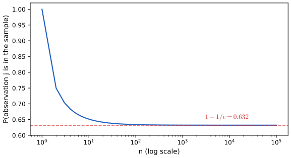
Exercise 5.2(g). \(1-(1-1/n)^n\) against \(n\) (log scale). The curve falls quickly from 1 and is flat at \(1-1/e=0.632\) from about \(n=100\) on; it decreases monotonically (Filling the gap 5.7). Code: fig_ex_2. Download: PDF · SVG(h)
R ch05_lab.R
set.seed(1)
ex2_store <- replicate(10000, any(sample(100, replace = TRUE) == 4))
mean(ex2_store)                              # close to 1 - (1 - 1/100)^100 = 0.634
Python ch05_lab.py
rng = np.random.default_rng(10)
store = np.array([np.any(rng.choice(100, 100, replace=True) == 4) for _ in range(10000)])
show("Exercise 2(h):", store.mean())                            # close to 0.634
# The book's line rng.choice(100, replace=True) draws ONE number, not a sample of 100:
rng = np.random.default_rng(10)
show("  as printed in the book:", np.mean([rng.choice(100, replace=True) == 4 for _ in range(10000)]))
R gives 0.6417 and Python 0.6362, both within two Monte Carlo standard errors (\(\sqrt{0.634\times0.366/10000}=0.0048\)) of 0.6340. See Notes on the book, 1 for the Python edition's version of this loop, and the demonstration.
Exercise 5.3. (a) Explain how k-fold cross-validation is carried out. (b) What are its advantages and disadvantages compared with (i) the validation set approach and (ii) LOOCV?
Solution
(a) Algorithm 5.1: partition the observations at random into \(k\) folds of nearly equal size; for each fold, fit on the other \(k-1\) folds and compute the error on the held-out fold; average the \(k\) errors (5.3).
(b)(i) Against the validation set: every observation is used both for fitting and for testing, each fit uses \((k-1)/k\) of the data rather than about half, so the estimate is less biased upwards, and it is far less variable (Figure 5.4 against Figure 5.2: a range of 0.2 against 6 at degree 2 on Auto). The costs are \(k\) fits instead of one and a slightly more involved procedure. (ii) Against LOOCV: \(k\) fits instead of \(n\), a large saving for slow methods (not for least squares, where (5.2) makes LOOCV cost one fit). k-fold CV is a little more biased upwards (its fits use fewer points), it depends on a random partition, and its variance may be lower or higher than LOOCV's depending on the method (Filling the gap 5.3).
Exercise 5.4. A learning method makes a prediction of \(Y\) at a particular value \(x_0\) of the predictor. Describe carefully how to estimate the standard deviation of that prediction.
Solution
Use the bootstrap (Algorithm 5.2) with the statistic "fit the method, predict at \(x_0\)". For \(r=1,\dots,B\): draw \(n\) rows with replacement, refit the method on them (including every tuning step, such as choosing a degree or \(\lambda\) by CV, so that its variability is counted), and record the prediction \(\hat f^{*r}(x_0)\). The standard deviation (5.8) of the \(B\) predictions estimates the standard error of \(\hat f(x_0)\). Two remarks. (1) This is the uncertainty of the estimated mean at \(x_0\); the uncertainty about a new response \(Y_0\) also includes the noise, roughly \(\sqrt{\SE^2+\hat\sigma^2}\), with \(\hat\sigma^2\) estimated from residuals (or by adding resampled residuals to each bootstrap prediction). (2) If the method is biased at \(x_0\), as flexible fits are near peaks or at the edges of the data, the bootstrap standard error does not see the bias.
Applied
Exercise 5.5. On the Default data, (a) fit a logistic regression of
defaultonincomeandbalance; (b) estimate its test error by the validation set approach (split, fit on the training half, classify the validation half by \(\hat p>0.5\), compute the misclassification rate); (c) repeat with three other splits and comment; (d) add a dummy variable forstudentand say whether it lowers the error.Solution
R ch05_lab.R
val_error <- function(seed, formula) {
  set.seed(seed)
  train <- sample(nrow(Default), nrow(Default) / 2)
  fit <- glm(formula, data = Default, subset = train, family = binomial)
  prob <- predict(fit, Default[-train, ], type = "response")
  mean(ifelse(prob > 0.5, "Yes", "No") != Default$default[-train])
}
ex5_two <- sapply(1:4, val_error, formula = default ~ income + balance)
ex5_three <- sapply(1:4, val_error, formula = default ~ income + balance + student)
round(rbind(ex5_two, ex5_three), 4)
Python ch05_lab.py
Default = isl_data("Default")
Default["y"] = (Default["default"] == "Yes").astype(float)
Default["stud"] = (Default["student"] == "Yes").astype(float)


def val_error(seed, cols):
    train, valid = train_test_split(Default, test_size=0.5, random_state=seed)
    fit = sm.GLM(train["y"], sm.add_constant(train[cols]), family=sm.families.Binomial()).fit()
    prob = fit.predict(sm.add_constant(valid[cols]))
    return np.mean((prob > 0.5) != (valid["y"] == 1))


ex5_two = [val_error(s, ["income", "balance"]) for s in (1, 2, 3, 4)]
ex5_three = [val_error(s, ["income", "balance", "stud"]) for s in (1, 2, 3, 4)]
show("Exercise 5, income + balance:", np.round(ex5_two, 4))
show("Exercise 5, + student:", np.round(ex5_three, 4))
validation error split 1 split 2 split 3 split 4 R, income + balance 0.0260 0.0242 0.0274 0.0254 R, + student 0.0256 0.0254 0.0280 0.0268 Python, income + balance 0.0250 0.0248 0.0248 0.0238 Python, + student 0.0262 0.0254 0.0252 0.0244 The error is about 2.5% and moves by about 0.3 percentage points from split to split (the splits differ between the languages, so do the numbers). For scale: 3.33% of the customers default, so always predicting "No" errs 3.3% of the time. Adding
studentdoes not lower the error: the changes, up or down by 0.1 point, are smaller than the split-to-split variation. (Student status matters for the default probability given balance, Chapter 4, but it rarely moves a customer across \(\hat p=0.5\).)Exercise 5.6. For the logistic regression of
defaultonincomeandbalance, compute the standard errors of the two slopes (a) from the usual formula of the fitted model and (b)–(c) by the bootstrap, and (d) compare.Solution
R ch05_lab.R
def_fit <- glm(default ~ income + balance, data = Default, family = binomial)
ex6_formula <- summary(def_fit)$coef[2:3, "Std. Error"]
ex6_formula                                  # income 4.985e-06, balance 2.274e-04
boot_fn_logit <- function(data, index) {
  coef(glm(default ~ income + balance, data = data, subset = index, family = binomial))[2:3]
}
set.seed(1)
boot_logit <- boot(Default, boot_fn_logit, R = 1000)
ex6_boot <- apply(boot_logit$t, 2, sd)
ex6_boot
Python ch05_lab.py
def logit_coef(D, idx):
    D_ = D.loc[idx]
    fit = sm.GLM(D_["y"], sm.add_constant(D_[["income", "balance"]]), family=sm.families.Binomial()).fit()
    return fit.params.to_numpy()[1:]


def_fit = sm.GLM(Default["y"], sm.add_constant(Default[["income", "balance"]]),
                 family=sm.families.Binomial()).fit()
ex6_formula = def_fit.bse.to_numpy()[1:]
ex6_boot, _ = boot_se(logit_coef, Default, B=1000, seed=0)
print("Exercise 6, formula SEs:", " ".join("%.4g" % v for v in ex6_formula))    # 4.985e-06 0.0002274
print("Exercise 6, bootstrap SEs:", " ".join("%.4g" % v for v in ex6_boot))
standard error incomebalanceformula (R and Python, equal to 4 digits) 4.985e-06 2.274e-04 bootstrap, \(B=1000\), R 4.866e-06 2.299e-04 bootstrap, \(B=1000\), Python 4.770e-06 2.306e-04 The two methods agree within a few percent, which is the size of the bootstrap's Monte Carlo error (about 2.2% for \(B=1000\)). The formula standard errors come from the Fisher information of the fitted logistic model; unlike the straight-line fit to Auto, here the bootstrap reveals no extra variability that the model misses.
Exercise 5.7. On the Weekly data, compute by hand the LOOCV error rate (5.4) of a logistic regression of
DirectiononLag1andLag2: (a) fit to all weeks; (b) fit without the first week; (c) classify the first week with that fit (Up if \(\hat P(\text{Up})>0.5\)) and check; (d) loop over all weeks, recording a 1 for each misclassified held-out week; (e) average and comment.Solution
R ch05_lab.R
wk_fit <- glm(Direction ~ Lag1 + Lag2, data = Weekly, family = binomial)
wk_fit_1 <- glm(Direction ~ Lag1 + Lag2, data = Weekly[-1, ], family = binomial)
ex7_p1 <- predict(wk_fit_1, Weekly[1, ], type = "response")
c(prob_up = ex7_p1, truth = as.character(Weekly$Direction[1]))   # predicts Up, truth Down
n_wk <- nrow(Weekly)
wrong <- numeric(n_wk)
for (i in seq_len(n_wk)) {
  fit_i <- glm(Direction ~ Lag1 + Lag2, data = Weekly[-i, ], family = binomial)
  p_up <- predict(fit_i, Weekly[i, ], type = "response")
  wrong[i] <- as.numeric((p_up > 0.5) != (Weekly$Direction[i] == "Up"))
}
ex7_loocv <- mean(wrong)
ex7_loocv                                    # 0.4500
Python ch05_lab.py
Weekly = isl_data("Weekly")
Xw = sm.add_constant(Weekly[["Lag1", "Lag2"]]).to_numpy()
yw = (Weekly["Direction"] == "Up").to_numpy(float)
binom = sm.families.Binomial()
fit_1 = sm.GLM(yw[1:], Xw[1:], family=binom).fit()
ex7_p1 = float(fit_1.predict(Xw[:1])[0])
show("Exercise 7(c), P(Up) for week 1:", ex7_p1)                # 0.5714 -> Up, but it went Down
wrong = np.empty(len(yw))
for i in range(len(yw)):
    keep = np.arange(len(yw)) != i
    p_up = sm.GLM(yw[keep], Xw[keep], family=binom).fit().predict(Xw[i:i + 1])[0]
    wrong[i] = (p_up > 0.5) != (yw[i] == 1)
ex7_loocv = wrong.mean()
show("Exercise 7, LOOCV error:", ex7_loocv)                     # 0.4500
(c) Without week 1, the fit gives \(\hat P(\text{Up})=0.5714\) for week 1, so it predicts Up; the market went Down, so week 1 is misclassified. (e) The LOOCV error rate is 0.4500 (490 mistakes in 1,089 weeks) in both languages: LOOCV involves no randomness. That is worse than the rule "always predict Up", whose error is 484/1089 = 0.444: the two lags carry no usable information about next week's direction, as Chapter 4 found.
Exercise 5.8. Simulate \(n=100\) points with \(X\sim\N(0,1)\) and \(Y=X-2X^2+\varepsilon\), \(\varepsilon\sim\N(0,1)\). (a) Give \(n\), \(p\) and the model. (b) Plot \(Y\) against \(X\). (c) Compute the LOOCV errors of polynomial regressions of degree 1 to 4. (d) Repeat with another seed. (e) Which model wins, and is that expected? (f) Do the significance tests of the coefficients agree with CV?
Solution
(a) \(n=100\) observations and \(p=1\) predictor; the model is \(Y=X-2X^2+\varepsilon\) with \(\varepsilon\sim\N(0,1)\) independent of \(X\). (b) An inverted parabola with its top near \(x=0.25\), \(y=0.125\), and noise of standard deviation 1 around it.
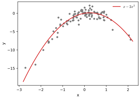
Exercise 5.8(b). The Python data ( default_rng(1)) with the true curve \(x-2x^2\). Code:fig_ex_8. Download: PDF · SVGR ch05_lab.R
set.seed(1)
x <- rnorm(100)
y <- x - 2 * x^2 + rnorm(100)
sim <- data.frame(x = x, y = y)
loocv_poly <- function(data) {
  sapply(1:4, function(d) cv.glm(data, glm(y ~ poly(x, d), data = data))$delta[1])
}
ex8_loocv <- loocv_poly(sim)
ex8_loocv                                    # degree 2 is best
set.seed(2)
all.equal(loocv_poly(sim), ex8_loocv)        # TRUE: LOOCV has no random element
ex8_pvalues <- summary(lm(y ~ poly(x, 4), data = sim))$coef[, "Pr(>|t|)"]
signif(ex8_pvalues, 3)                       # only the linear and quadratic terms are significant
Python ch05_lab.py
rng = np.random.default_rng(1)
x = rng.normal(size=100)
y = x - 2 * x ** 2 + rng.normal(size=100)
ex8_loocv = np.array([loocv_shortcut(Poly(d).fit(x).transform(x), y) for d in (1, 2, 3, 4)])
show("Exercise 8, LOOCV degrees 1-4:", np.round(ex8_loocv, 4))  # degree 2 is best
ex8_pvalues = sm.OLS(y, Poly(4).fit(x).transform(x)).fit().pvalues
print("Exercise 8(f), p-values:", " ".join("%.3g" % p for p in ex8_pvalues))
LOOCV degree 1 degree 2 degree 3 degree 4 R data ( set.seed(1))7.288 0.937 0.957 0.954 Python data ( default_rng(1))6.633 1.123 1.302 1.332 The two languages simulate different data from the same model, so the numbers differ. (d) Changing the seed after the data are simulated changes nothing: LOOCV involves no random choice, as the code confirms. (e) The quadratic has the smallest LOOCV error in both, as expected, since the truth is quadratic; the line is far worse, and the cubic and quartic pay a small price for their extra variance. (f) R data: the linear and quadratic terms have p-values of \(4.6\times10^{-9}\) and \(1.6\times10^{-43}\), the cubic and quartic 0.78 and 0.19, in line with CV. Python data: the cubic term has p = 0.28 but the quartic p = 0.023, nominally significant at 5% although the truth has no quartic term and CV prefers the quadratic. With four terms tested, one false positive at the 5% level is not surprising; a significance test of one coefficient and CV answer different questions, and here CV gives the better answer.
Exercise 5.9. For
medvin the Boston data: (a) estimate the mean \(\hat\mu\); (b) its standard error by the formula \(s/\sqrt n\); (c) by the bootstrap; (d) a 95% interval \(\hat\mu\pm2\SE\), compared with the t interval; (e)–(f) the median and its bootstrap standard error; (g)–(h) the 10th percentile and its bootstrap standard error.Solution
R ch05_lab.R
medv <- Boston$medv
ex9_mu <- mean(medv)
ex9_se <- sd(medv) / sqrt(length(medv))
c(mu = ex9_mu, se = ex9_se)                  # 22.533 0.409
set.seed(1)
boot_mean <- boot(medv, function(v, i) mean(v[i]), R = 1000)
ex9_se_boot <- sd(boot_mean$t[, 1])
ex9_ci_boot <- ex9_mu + c(-2, 2) * ex9_se_boot
ex9_ci_t <- t.test(medv)$conf.int
rbind(bootstrap = ex9_ci_boot, t.test = as.numeric(ex9_ci_t))
boot_med <- boot(medv, function(v, i) median(v[i]), R = 1000)
ex9_median <- median(medv)
ex9_se_median <- sd(boot_med$t[, 1])
boot_q10 <- boot(medv, function(v, i) quantile(v[i], 0.1), R = 1000)
ex9_q10 <- quantile(medv, 0.1)
ex9_se_q10 <- sd(boot_q10$t[, 1])
c(median = ex9_median, se = ex9_se_median, q10 = unname(ex9_q10), se = ex9_se_q10)
Python ch05_lab.py
Boston = isl_data("Boston")
medv = Boston["medv"].to_numpy(float)
ex9_mu, ex9_se = medv.mean(), medv.std(ddof=1) / np.sqrt(len(medv))
show("Exercise 9(a,b), mean and SE:", (round(ex9_mu, 4), round(ex9_se, 4)))   # 22.5328 0.4089
D9 = pd.DataFrame({"medv": medv})
stat = lambda f: (lambda D, idx: f(D["medv"].to_numpy()[idx]))      # noqa: E731
ex9_se_boot, _ = boot_se(stat(np.mean), D9, B=1000, seed=0)
ex9_ci_boot = (ex9_mu - 2 * ex9_se_boot, ex9_mu + 2 * ex9_se_boot)
ex9_ci_t = stats.t.interval(0.95, len(medv) - 1, loc=ex9_mu, scale=ex9_se)
show("Exercise 9(d), bootstrap and t intervals:", (np.round(ex9_ci_boot, 3), np.round(ex9_ci_t, 3)))
ex9_se_median, _ = boot_se(stat(np.median), D9, B=1000, seed=0)
ex9_q10 = np.percentile(medv, 10)
ex9_se_q10, _ = boot_se(stat(lambda v: np.percentile(v, 10)), D9, B=1000, seed=0)
show("Exercise 9(e-h), median, SE, 10th percentile, SE:",
     (np.median(medv), round(ex9_se_median, 4), ex9_q10, round(ex9_se_q10, 4)))
estimate formula SE bootstrap SE, R bootstrap SE, Python mean 22.533 0.4089 0.4107 0.4127 median 21.2 none 0.3770 0.3696 10th percentile 12.75 none 0.4926 0.5037 (a)–(c) The mean is 22.53 (thousands of dollars) with standard error 0.409; the bootstrap agrees within its Monte Carlo error, and the ideal bootstrap value is exactly 0.4085 (Filling the gap 5.6). (d) \(\hat\mu\pm2\SE_B\): [21.71, 23.35] in R and [21.71, 23.36] in Python, against the t interval [21.73, 23.34]: practically the same. (e)–(f) The median, 21.2, has a bootstrap standard error of about 0.37, smaller than that of the mean because
medvis skewed with a cluster of values capped at 50, which inflates the mean's variance but not the median's. (g)–(h) The 10th percentile, 12.75 (both languages use the same interpolation rule), is less precise, with a standard error of about 0.5, since fewer observations lie near it. For these two statistics no simple formula exists, and the bootstrap needs no new idea.
Demonstrations for this chapter
Each demonstration runs in the browser on the book's data and links back to these notes. The ▶ Demo boxes above open them already set to the case under discussion.
| Demonstration | What you can see | Sections and results |
|---|---|---|
| Validation set, LOOCV and k-fold CV on Auto | The fit and the held-out cars; the estimated test MSE against degree for every split drawn; the spread of the estimates at one degree; which degree each split picks. Presets: 1 one validation split; 2 ten splits (Figure 5.2); 3 LOOCV by one fit and by 392 refits; 4 nine 10-fold runs (Figure 5.4); 5 100 splits of each kind. | 5.1.1–5.1.4; Result 5.1, Filling the gap 5.1 |
| The bootstrap on Portfolio | The multiplicities of one resample; the risk curve and its minimum; the bootstrap histogram against the true sampling distribution; the standard error against \(B\). Presets: 1 one resample; 2 1,000 resamples; 3 against the truth (Figure 5.10); 4 how many resamples; 5 the risk curve. | 5.2; Result 5.2, Filling the gaps 5.5, 5.6 |
| Which observations a bootstrap sample contains | One sample as a grid of multiplicities; the inclusion probability against \(n\); the exact law of the number of distinct observations; Binomial against Poisson(1) copies. Presets: 1 \(n=3\); 2 \(n=5\); 3 \(n=100\); 4 \(n=1000\); 5 \(n=10{,}000\). | Result 5.3, Filling the gap 5.7, Exercise 5.2 |
Related demonstrations elsewhere on the site: the wrong and the right way to cross-validate and the .632 and .632+ bootstrap estimators (Statistical Learning: Theory and Methods), S-fold cross-validation (Foundations of Deep Learning), the bootstrap of a median (Statistical Methods for Modern Biology). The code for every figure of this page is code/ch05_resampling_methods.py; the lab is code/ch05_lab.R and code/ch05_lab.py (see the code index).
References
- James, G., Witten, D., Hastie, T. and Tibshirani, R. (2021). An Introduction to Statistical Learning with Applications in R, 2nd edition. Springer, New York. Chapter 5, pp. 197–223. www.statlearning.com.
- James, G., Witten, D., Hastie, T., Tibshirani, R. and Taylor, J. (2023). An Introduction to Statistical Learning with Applications in Python. Springer, Cham. Chapter 5, pp. 201–228.
- Arlot, S. and Celisse, A. (2010). A survey of cross-validation procedures for model selection. Statistics Surveys, 4, 40–79.
- Burman, P. (1989). A comparative study of ordinary cross-validation, v-fold cross-validation and the repeated learning-testing methods. Biometrika, 76(3), 503–514.
- Davison, A. C. and Hinkley, D. V. (1997). Bootstrap Methods and their Application. Cambridge University Press, Cambridge.
- Efron, B. (1979). Bootstrap methods: another look at the jackknife. Annals of Statistics, 7(1), 1–26.
- Efron, B. and Tibshirani, R. (1993). An Introduction to the Bootstrap. Chapman and Hall, New York.
- Hastie, T., Tibshirani, R. and Friedman, J. (2009). The Elements of Statistical Learning, 2nd edition. Springer, New York. Chapters 7 and 8.
- Stone, M. (1974). Cross-validatory choice and assessment of statistical predictions (with discussion). Journal of the Royal Statistical Society B, 36(2), 111–147.
- White, H. (1980). A heteroskedasticity-consistent covariance matrix estimator and a direct test for heteroskedasticity. Econometrica, 48(4), 817–838.
The numerical statements in the text (the shortcut (5.2) against refits for least squares and smoothing splines, the expected-error formula and the cross-validation simulation, the exact standard deviation of \(\hat\alpha\), the inclusion probabilities and the law of the number of distinct observations, the sandwich and bootstrap standard errors, and the lab and exercise results in both languages) were confirmed numerically.