Kernel Methods
Most models so far learned a parameter vector and then threw the training data away. Kernel methods keep the data: a prediction is a weighted combination of similarities between the new input and the training inputs. This chapter shows how that form arises from ridge regression (the dual representation), which functions qualify as similarities (valid kernels), how kernels give radial basis function and Nadaraya-Watson regression, and how placing a Gaussian distribution directly on functions gives Gaussian processes for regression and classification, with hyperparameters learned by the marginal likelihood.
Ch. 1 Introduction Ch. 2 Probability distributions Ch. 3 Linear regression Ch. 4 Linear classification Ch. 5 Neural networks Ch. 6 Kernel methods Ch. 7 Sparse kernel machines Ch. 8 Graphical models Ch. 9 Mixture models and EM Ch. 10 Approximate inference Ch. 11 Sampling methods Ch. 12 Continuous latent variables Ch. 13 Sequential data Ch. 14 Combining models
How to read these notes
They follow the book. Sections carry Bishop's numbers (6.1, 6.4.6, ...) and every displayed equation that appears in the book carries the book's own equation number, e.g. (6.66), so you can read these notes next to the book. Equations without a number are steps that the book skips.
Filling the gaps. Wherever the book says that something "can be shown", is "straightforward", follows from a matrix identity, or is left as an exercise, an orange Filling the gap box or a proof gives the full argument. Proofs and derivations start hidden: open one with its bar, or use the button below.
Figures and demonstrations. The numerical figures of the chapter are reproduced from scratch by the Python code. The ▶ Demo boxes open an interactive demonstration already set to the case being discussed. Standard identities (Woodbury, conditionals and marginals of a Gaussian, the linear-Gaussian model, matrix calculus) are proved once in the mathematical toolkit and linked where used.
Main reference
C. M. Bishop, Pattern Recognition and Machine Learning, Springer (2006), Chapter 6, pages 291–323. Section, equation, figure and exercise numbers below refer to this book. Further reading is listed in the references.
The explanations, derivations and code are my own; equations are cited by their numbers in the book.
The chapter at a glance
- 6.1 Regularised least squares can be rewritten in terms of the Gram matrix \(\mathbf{K}=\bm\Phi\bm\Phi^\T\) of inner products between feature vectors; the prediction becomes \(\mathbf{k}(\mathbf{x})^\T(\mathbf{K}+\lambda\mathbf{I}_N)^{-1}\mathbf{t}\). Only the kernel \(k(\mathbf{x},\mathbf{x}')\)
\({}=\bm\phi(\mathbf{x})^\T\bm\phi(\mathbf{x}')\) is needed, never \(\bm\phi\) itself. - 6.2 A function is a valid kernel exactly when all its Gram matrices are positive semidefinite. Ten closure rules (6.13)–(6.22) build new kernels from old ones; the Gaussian kernel has infinitely many features; generative models give kernels (including the Fisher kernel); the sigmoidal kernel is not valid.
- 6.3 Radial basis functions come from exact interpolation, from regularisation and from noisy inputs; normalising them gives the Nadaraya-Watson model, which is also what a Parzen estimate of the joint density implies for the regression function.
- 6.4 A Gaussian process is a Gaussian distribution over function values, specified by a kernel. Regression has a closed-form predictive distribution (6.66)–(6.67) at cost \(O(N^3)\); hyperparameters (length scales, noise, automatic relevance determination) are learned by maximising the marginal likelihood (6.69). For classification the posterior is not Gaussian; the Laplace approximation finds the unique mode by Newton-Raphson and gives a predictive probability and an approximate evidence (6.90). In the limit of infinitely many hidden units a Bayesian neural network is a Gaussian process.
Notation. Inputs \(\mathbf{x}_n\), targets \(t_n\), \(\mathbf{t}=(t_1,\dots,t_N)^\T\); feature map \(\bm\phi:\mathcal{X}\to\R^M\), design matrix \(\bm\Phi\) with \(n\)-th row \(\bm\phi(\mathbf{x}_n)^\T\); Gram matrix \(K_{nm}=k(\mathbf{x}_n,\mathbf{x}_m)\); \(\mathbf{k}(\mathbf{x})\) the vector with entries \(k(\mathbf{x}_n,\mathbf{x})\). A matrix \(\mathbf{A}\) is positive semidefinite (PSD) if \(\mathbf{v}^\T\mathbf{A}\mathbf{v}\ge0\) for all \(\mathbf{v}\), and positive definite (PD) if the inequality is strict for \(\mathbf{v}\ne\mathbf{0}\). This is not the same as having non-negative entries (Exercise 6.4).
Prerequisites. Linear regression and the equivalent kernel (Section 3.3.3), the conditional and marginal Gaussian (toolkit, linear-Gaussian model), the Woodbury identity (toolkit), logistic regression and the Laplace approximation (Section 4.4), Parzen density estimation (Section 2.5.1).
Printings. The text used here is a corrected printing. Where Bishop's errata list corrects an equation of this chapter (Figure 6.1, the sentence after (6.27), (6.40), (6.80), Exercises 6.16 and 6.23) the notes give the corrected form. Two further slips in the printed gradient formulas (6.91) and (6.94) are flagged where they occur; I found them by checking the formulas against finite differences.
Memory-based methods and the kernel trick
pp. 291–292 A parametric model (Chapters 3 to 5) compresses the training set into a parameter vector and then ignores it. A memory-based method keeps the training points, or some of them, and uses them again at prediction time: a Parzen density estimate puts a small bump on every training point, and a nearest-neighbour classifier copies the label of the closest one. Such methods need a way to measure similarity between two inputs, and are cheap to "train" but costly to evaluate.
Many linear models can be rewritten so that predictions also have this form. The key object is the kernel
\[ k(\mathbf{x},\mathbf{x}')=\bm\phi(\mathbf{x})^\T\bm\phi(\mathbf{x}'), \tag{6.1} \]an inner product in a feature space. It is symmetric, \(k(\mathbf{x},\mathbf{x}')\)
A kernel that depends only on the difference of its arguments, \(k(\mathbf{x}-\mathbf{x}')\), is stationary (unchanged by translating both inputs); one that depends only on \(\|\mathbf{x}-\mathbf{x}'\|\) is homogeneous or a radial basis function (Section 6.3).
6.1 Dual representations
pp. 293–294 Consider regularised least squares with a fixed feature map \(\bm\phi\) and \(\lambda\ge0\),
\[ J(\mathbf{w})=\frac12\sum_{n=1}^{N}\{\mathbf{w}^\T\bm\phi(\mathbf{x}_n)-t_n\}^2+\frac{\lambda}{2}\mathbf{w}^\T\mathbf{w}. \tag{6.2} \]Filling the gap 6.1: from (6.2) to the dual problem (6.3) to (6.9) pp. 293–294, (6.3)–(6.9)
The book states each step in one line. For \(\lambda>0\) every step below is an equality; the one place where care is needed is the passage from the stationarity condition on \(\mathbf{a}\) to (6.8).
Derivation
The solution lies in the span of the features (6.3). In matrix form \(J(\mathbf{w})\)
The coefficients \(a_n\) are minus the residuals divided by \(\lambda\). (The book's sentence before (6.8) is corrected in the errata to "Using (6.3) to eliminate \(\mathbf{w}\) from (6.4) and solving for \(\mathbf{a}\) we obtain".)
Substituting \(\mathbf{w}=\bm\Phi^\T\mathbf{a}\) into \(J\). We have \(\bm\Phi\mathbf{w}\)
where \(K_{nm}\)
Solving for \(\mathbf{a}\) (6.8). The gradient of (6.7) is \(\mathbf{K}\mathbf{K}\mathbf{a}\)
The inverse exists for \(\lambda>0\) because \(\mathbf{K}\) is PSD, so \(\mathbf{K}+\lambda\mathbf{I}\) has eigenvalues \(\ge\lambda>0\). It is the same \(\mathbf{a}\) that comes directly from (6.3)–(6.4): \(\lambda\mathbf{a}\)
Prediction (6.9). For a new \(\mathbf{x}\), \(y(\mathbf{x})\)
The prediction is a linear combination of the training targets whose weights, \(\mathbf{k}(\mathbf{x})^\T(\mathbf{K}+\lambda\mathbf{I})^{-1}\), are the equivalent kernel of Section 3.3.3.
Agreement with the primal solution. The usual ridge solution is \(\mathbf{w}\)
Filling the gap 6.2: primal or dual? The cost comparison p. 294
The book remarks that the dual needs an \(N\times N\) inverse where the primal needs an \(M\times M\) one, so the dual "does not seem to be particularly useful" when \(N\gg M\); its advantage is that it never needs \(\bm\phi\).
Counting operations
| Primal (weights \(\mathbf{w}\)) | Dual (coefficients \(\mathbf{a}\)) | |
|---|---|---|
| Build the matrix | \(\bm\Phi^\T\bm\Phi\): \(O(NM^2)\) | Gram matrix \(\mathbf{K}\): \(O(N^2)\) kernel evaluations |
| Solve once | \(M\times M\) system: \(O(M^3)\) | \(N\times N\) system: \(O(N^3)\) |
| Predict one point | \(\mathbf{w}^\T\bm\phi(\mathbf{x})\): \(O(M)\) | \(\mathbf{a}^\T\mathbf{k}(\mathbf{x})\): \(O(N)\) kernel evaluations |
| Storage | \(\mathbf{w}\): \(M\) numbers | \(\mathbf{a}\) and all \(N\) training inputs |
A Cholesky factorisation of a symmetric positive definite \(n\times n\) matrix costs \(n^3/3\) multiplications, and the two triangular solves afterwards cost \(O(n^2)\), so "inverting" is done once. If \(M
Other models have duals too. The perceptron's weight vector is a sum of the misclassified feature vectors, so it also has a dual form in which \(\bm\phi\) appears only through \(k\) (Exercise 6.2); and in Chapter 7 the dual is the main tool for support vector machines. Exercise 6.16 shows the general reason: whenever the objective depends on \(\mathbf{w}\) only through the values \(\mathbf{w}^\T\bm\phi(\mathbf{x}_n)\) and a monotone function of \(\mathbf{w}^\T\mathbf{w}\), the minimiser is a linear combination of the \(\bm\phi(\mathbf{x}_n)\) (the representer theorem, Kimeldorf and Wahba 1971). In Section 6.4 the same formula (6.9) reappears as the mean of a Gaussian process.
6.2 Constructing kernels
pp. 294–299 There are two ways to obtain a kernel: choose a feature map and compute the inner product, or write down a function \(k\) directly and make sure that it is an inner product of some feature map. The first route, with \(M\) basis functions \(\phi_i\), gives
\[ k(x,x')=\bm\phi(x)^\T\bm\phi(x')=\sum_{i=1}^{M}\phi_i(x)\phi_i(x'), \tag{6.10} \]shown in Figure 6.1 for polynomial, Gaussian and logistic-sigmoid basis functions on a one-dimensional input space. For the second route, a simple example is
\[ k(\mathbf{x},\mathbf{z})=(\mathbf{x}^\T\mathbf{z})^2. \tag{6.11} \]For \(\mathbf{x}=(x_1,x_2)\) expand the square:
\[ (\mathbf{x}^\T\mathbf{z})^2=(x_1z_1+x_2z_2)^2=x_1^2z_1^2+2x_1z_1x_2z_2+x_2^2z_2^2=(x_1^2,\sqrt2\,x_1x_2,x_2^2)(z_1^2,\sqrt2\,z_1z_2,z_2^2)^\T=\bm\phi(\mathbf{x})^\T\bm\phi(\mathbf{z}). \tag{6.12} \]The feature map \(\bm\phi(\mathbf{x})\)
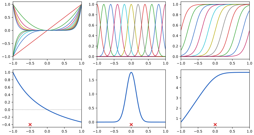
fig6_1. Download: PDF · SVGDefinition 6.1 (kernel, Gram matrix, valid kernel) pp. 294–295
A kernel is a symmetric function \(k:\mathcal{X}\times\mathcal{X}\to\R\). For points \(\mathbf{x}_1,\dots,\mathbf{x}_N\in\mathcal{X}\) its Gram matrix is \(K_{nm}=k(\mathbf{x}_n,\mathbf{x}_m)\). The kernel is valid (positive semidefinite) if there is a real vector space \(\mathcal{H}\) with an inner product \(\langle\cdot,\cdot\rangle\) and a map \(\bm\phi:\mathcal{X}\to\mathcal{H}\) with \(k(\mathbf{x},\mathbf{x}')\)
Result 6.1 (valid kernels are exactly those with positive semidefinite Gram matrices) p. 295
A symmetric function \(k\) is a valid kernel if and only if, for every finite set of points \(\mathbf{x}_1,\dots,\mathbf{x}_N\) (repeats allowed) and every \(\mathbf{a}\in\R^N\),
\[ \sum_{n=1}^{N}\sum_{m=1}^{N}a_na_m\,k(\mathbf{x}_n,\mathbf{x}_m)=\mathbf{a}^\T\mathbf{K}\mathbf{a}\ge0, \]that is, if every Gram matrix is positive semidefinite. Equivalently, all eigenvalues of every Gram matrix are \(\ge0\). A necessary consequence is the Cauchy-Schwarz inequality \(k(\mathbf{x},\mathbf{x}')^2\)
Proof
(valid \(\Rightarrow\) PSD). Symmetry of \(k\) is symmetry of the inner product, and
\(\mathbf{a}^\T\mathbf{K}\mathbf{a}\)
(PSD \(\Rightarrow\) valid), finite set. For one fixed set of \(N\) points, \(\mathbf{K}=\mathbf{U}\bm\Lambda\mathbf{U}^\T\) with \(\bm\Lambda\ge0\) (spectral theorem), and the vectors \(\bm\phi_n\)
(PSD \(\Rightarrow\) valid), whole space (the reproducing-kernel construction of Aronszajn, 1950). Let \(\mathcal{H}_0\) be the vector space of functions \(f=\sum_{i=1}^{p}\alpha_ik(\cdot,\mathbf{x}_i)\), and define \(\langle f,g\rangle\)
Remark. "Positive semidefinite" does not mean "entries \(\ge0\)": the matrix \(\begin{pmatrix}1&2\\2&1\end{pmatrix}\) has positive entries and eigenvalues \(3,-1\), while \(\begin{pmatrix}2&-1\\-1&2\end{pmatrix}\) has a negative entry and eigenvalues \(1,3\) (Exercise 6.4).
Result 6.2 (Mercer's theorem, statement) p. 295 (cited via Shawe-Taylor and Cristianini, 2004)
Let \(\mathcal{X}\subset\R^D\) be compact, \(\mu\) a finite measure on \(\mathcal{X}\) with full support, and \(k\) a continuous symmetric function with \(\iint k(\mathbf{x},\mathbf{x}')f(\mathbf{x})f(\mathbf{x}')\,\d\mu\,\d\mu\)
with absolute and uniform convergence. So \(\bm\phi(\mathbf{x})\)
What is proved, and why it matters here
The proof (Mercer, 1909; see Rasmussen and Williams, 2006, Section 4.3) uses the spectral theorem for compact self-adjoint operators plus Dini's theorem for the uniform convergence; I do not repeat it. Two connections are worth recording.
Gram matrices. If every Gram matrix is PSD, approximate the double integral by a Riemann sum over a fine partition of \(\mathcal{X}\) (for continuous \(f\) and \(k\) the sums converge): each sum is \(\sum_{n,m}a_na_mk(\mathbf{x}_n,\mathbf{x}_m)\) with \(a_n=f(\mathbf{x}_n)\mu(\text{cell}_n)\), which is \(\ge0\), so the integral is \(\ge0\) for continuous \(f\), hence for all of \(L^2\) by density. Conversely, if the integral condition holds, choose \(f\) as a sharply peaked bump at each \(\mathbf{x}_n\) with weight \(a_n\) and let the bumps shrink; continuity of \(k\) gives \(\mathbf{a}^\T\mathbf{K}\mathbf{a}\ge0\).
Functions drawn from a Gaussian process. If \(\xi_i\sim\N(0,1)\) are independent, then \(y(\mathbf{x})\)
The Gram test is hard to apply directly, so kernels are built from simpler ones.
Result 6.3 (closure rules: techniques for constructing new kernels) p. 296, (6.13)–(6.22); Exercises 6.5–6.9
Let \(k_1,k_2\) be valid kernels on \(\mathcal{X}\). Then each of the following is a valid kernel:
\[ \begin{align} k(\mathbf{x},\mathbf{x}')&=c\,k_1(\mathbf{x},\mathbf{x}') \tag{6.13}\\ k(\mathbf{x},\mathbf{x}')&=f(\mathbf{x})\,k_1(\mathbf{x},\mathbf{x}')\,f(\mathbf{x}') \tag{6.14}\\ k(\mathbf{x},\mathbf{x}')&=q\big(k_1(\mathbf{x},\mathbf{x}')\big) \tag{6.15}\\ k(\mathbf{x},\mathbf{x}')&=\exp\big(k_1(\mathbf{x},\mathbf{x}')\big) \tag{6.16}\\ k(\mathbf{x},\mathbf{x}')&=k_1(\mathbf{x},\mathbf{x}')+k_2(\mathbf{x},\mathbf{x}') \tag{6.17}\\ k(\mathbf{x},\mathbf{x}')&=k_1(\mathbf{x},\mathbf{x}')\,k_2(\mathbf{x},\mathbf{x}') \tag{6.18}\\ k(\mathbf{x},\mathbf{x}')&=k_3\big(\bm\phi(\mathbf{x}),\bm\phi(\mathbf{x}')\big) \tag{6.19}\\ k(\mathbf{x},\mathbf{x}')&=\mathbf{x}^\T\mathbf{A}\mathbf{x}' \tag{6.20}\\ k(\mathbf{x},\mathbf{x}')&=k_a(\mathbf{x}_a,\mathbf{x}_a')+k_b(\mathbf{x}_b,\mathbf{x}_b') \tag{6.21}\\ k(\mathbf{x},\mathbf{x}')&=k_a(\mathbf{x}_a,\mathbf{x}_a')\,k_b(\mathbf{x}_b,\mathbf{x}_b') \tag{6.22} \end{align} \]where \(c\ge0\) (the book writes \(c>0\)), \(f\) is any real function, \(q\) is a polynomial with non-negative coefficients, \(\bm\phi:\mathcal{X}\to\R^M\) and \(k_3\) is a valid kernel on \(\R^M\), \(\mathbf{A}\) is symmetric positive semidefinite, \(\mathbf{x}=(\mathbf{x}_a,\mathbf{x}_b)\) with possibly overlapping parts, and \(k_a,k_b\) are valid kernels on the respective spaces.
Proof (each rule, by the Gram criterion of Result 6.1)
Fix points \(\mathbf{x}_1,\dots,\mathbf{x}_N\), write \(\mathbf{K}_1,\mathbf{K}_2\) for the Gram matrices of \(k_1,k_2\) (both PSD), and let \(\mathbf{a}\in\R^N\) be arbitrary. Symmetry of each new function is obvious in every case.
(6.13). The Gram matrix is \(c\mathbf{K}_1\) and \(\mathbf{a}^\T(c\mathbf{K}_1)\mathbf{a}\)
(6.14). With \(\mathbf{D}\)
(6.17). \(\mathbf{a}^\T(\mathbf{K}_1+\mathbf{K}_2)\mathbf{a}\)
(6.18). The Gram matrix is the entrywise (Hadamard) product \(\mathbf{K}_1\circ\mathbf{K}_2\). Write \(\mathbf{K}_1\)
(6.15). Let \(q(z)=\sum_{j=0}^{J}c_jz^j\) with all \(c_j\ge0\). The constant function \(1\) is a valid kernel (feature \(\phi\equiv1\)). By (6.18) and induction \(k_1^j\) is valid for each \(j\ge1\) (and \(k_1^0=1\)); by (6.13) \(c_jk_1^j\) is valid; by (6.17) the sum is valid.
(6.16). The partial sums \(s_J=\sum_{j=0}^{J}k_1^j/j!\) are of the form (6.15), hence valid, and \(s_J(\mathbf{x},\mathbf{x}')\)
(6.19). The Gram matrix of \(k\) at \(\mathbf{x}_1,\dots,\mathbf{x}_N\) is the Gram matrix of \(k_3\) at the points \(\bm\phi(\mathbf{x}_1),\dots,\bm\phi(\mathbf{x}_N)\in\R^M\), which is PSD (repeated points are allowed). (Feature map: \(\bm\psi\circ\bm\phi\), with \(\bm\psi\) a feature map of \(k_3\).)
(6.20). Write \(\mathbf{A}=\mathbf{L}^\T\mathbf{L}\) (for instance \(\mathbf{L}=\mathbf{A}^{1/2}\), from the spectral decomposition, which exists since the eigenvalues are \(\ge0\)). Then \(\mathbf{x}^\T\mathbf{A}\mathbf{x}'\)
(6.21), (6.22). The function \(\tilde k_a(\mathbf{x},\mathbf{x}')\)
Remark: what is not allowed. The difference \(k_1-k_2\) need not be valid (take \(k_2=2k_1\), then \(-k_1\) has a negative diagonal), and a general function \(g(k_1)\) of a kernel is valid only under conditions such as those of (6.15)–(6.16). Constants \(c<0\) are excluded in (6.13).
With these rules the polynomial kernels above are valid: \((\mathbf{x}^\T\mathbf{x}')^M\) by (6.18) repeatedly, \((\mathbf{x}^\T\mathbf{x}'+c)^M\) by (6.15) with \(q(z)=(z+c)^M\).
The Gaussian kernel
pp. 296–297; Exercise 6.11 The most used kernel is the "Gaussian"
\[ k(\mathbf{x},\mathbf{x}')=\exp\!\big(-\|\mathbf{x}-\mathbf{x}'\|^2/2\sigma^2\big). \tag{6.23} \]It is not a probability density here, so the normalising constant is omitted.
Filling the gap 6.3: the Gaussian kernel is valid, with infinitely many features pp. 296–297, (6.24)–(6.26); Exercise 6.11
The book expands the square and applies (6.14) and (6.16). The statement that the feature space is infinite-dimensional is left as an exercise; here is the explicit feature map.
Derivation
Validity. Expand \(\|\mathbf{x}-\mathbf{x}'\|^2\)
The linear kernel \(\mathbf{x}^\T\mathbf{x}'/\sigma^2\) is valid (6.13), so the middle factor is valid by (6.16), and multiplying by \(f(\mathbf{x})\)
Explicit features (Exercise 6.11). Expand the middle factor as a power series, and the power \((\mathbf{x}^\T\mathbf{x}')^j\) by the multinomial theorem. For a multi-index \(\bm\alpha=(\alpha_1,\dots,\alpha_D)\) of non-negative integers put \(|\bm\alpha|=\sum_d\alpha_d\), \(\bm\alpha!=\prod_d\alpha_d!\), \(\mathbf{x}^{\bm\alpha}=\prod_dx_d^{\alpha_d}\). Then \((\mathbf{x}^\T\mathbf{x}')^j\)
Hence \(k(\mathbf{x},\mathbf{x}')\)
For \(D=1\): \(\phi_j(x)\)
Kernel substitution (6.26). If \(\kappa\) is any valid kernel, then \[ \exp\Big\{-\frac1{2\sigma^2}\big(\kappa(\mathbf{x},\mathbf{x})+\kappa(\mathbf{x}',\mathbf{x}')-2\kappa(\mathbf{x},\mathbf{x}')\big)\Big\} \]
is valid by the same argument: \(\kappa(\mathbf{x},\mathbf{x}')/\sigma^2\) is valid, so \(\exp\) of it is valid (6.16), and the two outer factors are of the form (6.14). The expression in braces is \(\|\bm\varphi(\mathbf{x})\)
Kernels for non-vector inputs
p. 297; Exercise 6.12 Kernels can be defined on graphs, sets, strings or documents. For subsets \(A_1,A_2\) of a fixed finite set \(D\),
\[ k(A_1,A_2)=2^{|A_1\cap A_2|}, \tag{6.27} \]where \(|A|\) is the number of elements of \(A\) (the first printing says "subsets"; the errata corrects it). It is valid: take the feature space \(\R^{2^{|D|}}\) indexed by the subsets \(U\subseteq D\), with \(\phi_U(A)=1\) if \(U\subseteq A\) and \(0\) otherwise (6.95). Then \(\bm\phi(A_1)^\T\bm\phi(A_2)\) counts the subsets \(U\) with \(U\subseteq A_1\) and \(U\subseteq A_2\), that is \(U\subseteq A_1\cap A_2\), and a set with \(|A_1\cap A_2|\) elements has \(2^{|A_1\cap A_2|}\) subsets.
Kernels from probabilistic generative models
pp. 297–298, (6.28)–(6.31) Generative models handle missing data and variable-length sequences naturally; discriminative models usually classify better. One way to combine them is to let a generative model define the kernel and then use it in a discriminative method (Haussler, 1999). For a density \(p\),
\[ k(\mathbf{x},\mathbf{x}')=p(\mathbf{x})\,p(\mathbf{x}'), \tag{6.28} \]is valid, an inner product in a one-dimensional feature space with \(\phi(\mathbf{x})=p(\mathbf{x})\): two inputs are similar if both are probable. Using (6.13) and (6.17), with weights \(p(i)\ge0\) summing to one,
\[ k(\mathbf{x},\mathbf{x}')=\sum_{i}p(\mathbf{x}\given i)\,p(\mathbf{x}'\given i)\,p(i), \tag{6.29} \]whose feature map is \(\phi_i(\mathbf{x})\)
the inner product in \(L^2(p(\mathbf{z})\d\mathbf{z})\) of the functions \(\mathbf{z}\mapsto p(\mathbf{x}\given\mathbf{z})\), hence valid. For sequences \(\mathbf{X}=(\mathbf{x}_1,\dots,\mathbf{x}_L)\) with a hidden Markov model (Section 13.2),
\[ k(\mathbf{X},\mathbf{X}')=\sum_{\mathbf{Z}}p(\mathbf{X}\given\mathbf{Z})\,p(\mathbf{X}'\given\mathbf{Z})\,p(\mathbf{Z}), \tag{6.31} \]is (6.29) with the hidden state sequence \(\mathbf{Z}\) as the index: both observed sequences are generated by the same hidden path. It can be computed with a forward recursion on the product of the two emission models (a pair HMM), and extended to sequences of different length.
The Fisher kernel
pp. 298–299, (6.32)–(6.36); Exercises 6.13, 6.14 Given a parametric model \(p(\mathbf{x}\given\bm\theta)\), the Fisher score \(\mathbf{g}(\bm\theta,\mathbf{x})\)
with the expectation under \(p(\mathbf{x}\given\bm\theta)\).
Filling the gap 6.4: validity, invariance and the sample versions of the Fisher kernel pp. 298–299; Exercise 6.13
The book says that the Fisher information matrix makes the kernel invariant to re-parametrisation, and that its sample version whitens the scores. Here are the arguments.
Derivation
Validity. \(\mathbf{F}\) is a second-moment matrix, hence symmetric PSD; assume it is invertible. Then \(\mathbf{F}^{-1}\) is symmetric PSD and (6.33) is of the form (6.20) applied to the features \(\mathbf{g}\), hence valid. Equivalently, the feature map is the whitened score \(\mathbf{F}^{-1/2}\mathbf{g}\).
The scores have mean zero under the model: \(\E[\mathbf{g}]\)
Invariance (Exercise 6.13). Let \(\bm\psi=\bm\psi(\bm\theta)\) be an invertible differentiable reparametrisation, with Jacobian \(\mathbf{J}=\partial\bm\theta/\partial\bm\psi\) (square, invertible). By the chain rule the new score is \(\mathbf{g}_\psi=\mathbf{J}^\T\mathbf{g}_\theta\). Hence \(\mathbf{F}_\psi\)
Without \(\mathbf{F}^{-1}\) (the kernel (6.36)) the value \(\mathbf{g}^\T\mathbf{J}\mathbf{J}^\T\mathbf{g}'\) changes under reparametrisation.
Practical versions. Replacing the expectation by an average over the data gives
\[ \mathbf{F}\simeq\frac1N\sum_{n=1}^{N}\mathbf{g}(\bm\theta,\mathbf{x}_n)\mathbf{g}(\bm\theta,\mathbf{x}_n)^\T, \tag{6.35} \]the sample covariance of the scores when their mean is about zero, so the Fisher kernel then whitens the scores (Section 12.1.3). Dropping \(\mathbf{F}\) altogether gives the simpler, non-invariant kernel
\[ k(\mathbf{x},\mathbf{x}')=\mathbf{g}(\bm\theta,\mathbf{x})^\T\mathbf{g}(\bm\theta,\mathbf{x}'). \tag{6.36} \]Example (Exercise 6.14). For \(p(\mathbf{x}\given\bm\mu)\)
Fisher kernels have been used for document retrieval (Hofmann, 2000) and, with HMMs, for biological sequences and speech.
The sigmoidal kernel is not valid
p. 299, (6.37) The sigmoidal kernel
\[ k(\mathbf{x},\mathbf{x}')=\tanh\big(a\,\mathbf{x}^\T\mathbf{x}'+b\big) \tag{6.37} \]gives support-vector expansions a superficial resemblance to neural networks (Vapnik, 1995) but, as the book says, its Gram matrix is in general not positive semidefinite. Two explicit counterexamples:
Filling the gap 6.5: the sigmoidal kernel violates positive semidefiniteness p. 299
Counterexamples
(i) \(b<0\). A valid kernel has \(k(\mathbf{x},\mathbf{x})\)
(ii) \(b=0\), one-dimensional input, \(a=1\). Take \(x_1=1\), \(x_2=2\):
\[ \mathbf{K}=\begin{pmatrix}\tanh1&\tanh2\\\tanh2&\tanh4\end{pmatrix}\approx\begin{pmatrix}0.7616&0.9640\\0.9640&0.9993\end{pmatrix},\qquad\det\mathbf{K}=\tanh1\tanh4-\tanh^22\approx-0.168<0, \]so \(\mathbf{K}\) has eigenvalues of opposite sign, approximately \(-0.091\) and \(1.852\). The Cauchy-Schwarz inequality \(k(1,2)^2\le k(1,1)k(2,2)\) is violated. (Small \(a\) also fails: \(\det\approx-12a^4\) to leading order, from the expansion \(\tanh z=z-z^3/3+\cdots\).) For \(a=b=1\), a numerical search over three-point sets found, for example, \(x=(-1.25,\,0.09,\,2.97)\) with smallest eigenvalue about \(-0.79\).
So (6.37) is a valid kernel only for special parameter choices and data sets, and the SVM objective is then not convex. The deeper connection between neural networks and kernels is the Gaussian-process limit of Section 6.4.7, where the kernel that arises is a legitimate one.
6.3 Radial basis function networks
pp. 299–301 A radial basis function (RBF) depends only on the distance from a centre \(\bm\mu_j\): \(\phi_j(\mathbf{x})=h(\|\mathbf{x}-\bm\mu_j\|)\). Linear models in such basis functions (Chapter 3) are called RBF networks. Three different motivations lead to them.
Exact interpolation (Powell, 1987). Given noise-free data \(\{\mathbf{x}_n,t_n\}\), look for a function through every point, with one basis function centred on each input,
\[ f(\mathbf{x})=\sum_{n=1}^{N}w_n\,h(\|\mathbf{x}-\mathbf{x}_n\|). \tag{6.38} \]Requiring \(f(\mathbf{x}_m)=t_m\) gives \(N\) linear equations \(\mathbf{H}\mathbf{w}=\mathbf{t}\), \(H_{mn}=h(\|\mathbf{x}_m-\mathbf{x}_n\|)\), for \(N\) unknowns, solvable when \(\mathbf{H}\) is invertible (for the Gaussian \(h\), \(\mathbf{H}\) is a Gram matrix of the Gaussian kernel, positive definite for distinct points). With noisy targets this over-fits: the fit passes through the noise (the \(\lambda\to0\) limit of (6.9) with \(\mathbf{K}=\mathbf{H}\)).
Regularisation theory (Poggio and Girosi, 1990). If the sum of squares is penalised by a differential operator, the optimal function is an expansion in the Green's functions of the operator, one per data point; for an isotropic operator they are radial, and the penalty means the fit no longer interpolates.
Noisy inputs (Webb, 1994; Bishop, 1995). If the input is corrupted, \(\mathbf{x}_n\to\mathbf{x}_n+\bm\xi\) with \(\bm\xi\sim\nu\), the expected sum of squares is
\[ E=\frac12\sum_{n=1}^{N}\int\{y(\mathbf{x}_n+\bm\xi)-t_n\}^2\,\nu(\bm\xi)\,\d\bm\xi. \tag{6.39} \]Filling the gap 6.6: minimising (6.39) gives normalised basis functions pp. 300, (6.39)–(6.41); Exercise 6.17
The book says "using the calculus of variations". Errata: the sentence after (6.39) should read "with respect to the function \(y(\mathbf{x})\)", and the left side of (6.40) is \(y(\mathbf{x})\), not \(y(\mathbf{x}_n)\). Here is the argument, both from first principles and as an Euler-Lagrange equation.
Derivation
Change variable. In the \(n\)-th term put \(\mathbf{z}=\mathbf{x}_n+\bm\xi\), \(\bm\xi=\mathbf{z}-\mathbf{x}_n\) (unit Jacobian):
\[ E[y]=\frac12\int\Big\{\sum_{n=1}^{N}\nu(\mathbf{z}-\mathbf{x}_n)\big(y(\mathbf{z})-t_n\big)^2\Big\}\d\mathbf{z}. \]Functional derivative. The integrand depends on \(y\) only through its value \(y(\mathbf{z})\) at the same point (no derivatives of \(y\)). Perturb \(y\to y+\epsilon\eta\); the coefficient of \(\epsilon\) in \(E[y+\epsilon\eta]\) is
\[ \int\eta(\mathbf{z})\sum_{n}\nu(\mathbf{z}-\mathbf{x}_n)\big(y(\mathbf{z})-t_n\big)\d\mathbf{z}=0\quad\text{for every }\eta, \]so by the fundamental lemma of the calculus of variations (choose \(\eta\) a narrow bump at any \(\mathbf{z}\), as in the toolkit) the integrand's bracket vanishes for each \(\mathbf{z}\): \(\sum_n\nu(\mathbf{z}-\mathbf{x}_n)(y(\mathbf{z})-t_n)\)
It is a minimum. For each fixed \(\mathbf{z}\), the integrand is a quadratic in the number \(y(\mathbf{z})\) with positive leading coefficient \(\sum_n\nu(\mathbf{z}-\mathbf{x}_n)\) (assuming it is positive), so the stationary value is the pointwise minimum and hence the global minimum of \(E\). The solution is a weighted mean of the targets with weights \(\nu(\mathbf{z}-\mathbf{x}_n)\): the noise density decides how much each target counts at \(\mathbf{z}\).
Properties. One basis function sits on every data point. If \(\nu\) is isotropic, \(\nu(\bm\xi)=\nu(\|\bm\xi\|)\), the functions \(h\) are radial. And \(\sum_nh(\mathbf{x}-\mathbf{x}_n)=1\) for every \(\mathbf{x}\) (the basis functions are normalised): the prediction is always a convex combination of the targets, so it stays within their range.∎
The effect of normalisation is shown in Figure 6.2. Without it, the model output (a linear combination) decays to zero (or to the bias parameter) far from every centre; with it, the nearest centres dominate and the prediction approaches the target of the closest point. This is the Nadaraya-Watson model of the next subsection, which appears here as the solution for noisy inputs and there as the solution of kernel density estimation.
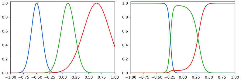
fig6_2. Download: PDF · SVGFewer basis functions than data points. Because (6.38) and (6.40) have one basis function per data point, evaluating them is expensive. Broomhead and Lowe (1988), Moody and Darken (1989) and Poggio and Girosi (1990) keep the radial form but use \(M
6.3.1 Nadaraya-Watson model
pp. 301–303, (6.42)–(6.48) In Section 3.3.3 the prediction of linear regression was a linear combination of the training targets with the equivalent kernel (3.62). A different route to such a form starts from density estimation. Model the joint density of input and target by a Parzen estimator (Section 2.5.1) with one component \(f\) on every data point,
\[ p(\mathbf{x},t)=\frac1N\sum_{n=1}^{N}f(\mathbf{x}-\mathbf{x}_n,\,t-t_n), \tag{6.42} \]and take as the regression function the conditional mean \(y(\mathbf{x})\)
Filling the gap 6.7: the Nadaraya-Watson formula pp. 301–302, (6.43)–(6.47); Exercise 6.18
The book applies "a simple change of variable". Here it is, with the conditional distribution as well.
Derivation
Substituting (6.42) into numerator and denominator, the factor \(1/N\) cancels and the integrals are taken term by term:
\[ y(\mathbf{x})=\frac{\sum_n\int t\,f(\mathbf{x}-\mathbf{x}_n,t-t_n)\,\d t}{\sum_m\int f(\mathbf{x}-\mathbf{x}_m,t-t_m)\,\d t}. \tag{6.43} \]Assume each component has zero mean in \(t\) at every \(\mathbf{x}\): \(\int f(\mathbf{x},t)\,t\,\d t=0\) (6.44). In the numerator substitute \(s=t-t_n\):
\[ \int t\,f(\mathbf{x}-\mathbf{x}_n,t-t_n)\,\d t=\int(s+t_n)f(\mathbf{x}-\mathbf{x}_n,s)\,\d s=\underbrace{\int s\,f(\mathbf{x}-\mathbf{x}_n,s)\,\d s}_{=0\text{ by (6.44)}}+t_n\int f(\mathbf{x}-\mathbf{x}_n,s)\,\d s=t_n\,g(\mathbf{x}-\mathbf{x}_n), \]with \(g(\mathbf{x})\)
and the kernel sums to one, \(\sum_nk(\mathbf{x},\mathbf{x}_n)=1\). The weights \(k\) are the same as the normalised basis functions (6.41), with \(g\) in the role of the input-noise density \(\nu\). The same shift gives the full conditional distribution
\[ p(t\given\mathbf{x})=\frac{p(t,\mathbf{x})}{\int p(t,\mathbf{x})\,\d t}=\frac{\sum_nf(\mathbf{x}-\mathbf{x}_n,t-t_n)}{\sum_m\int f(\mathbf{x}-\mathbf{x}_m,t-t_m)\,\d t}=\sum_n k(\mathbf{x},\mathbf{x}_n)\,\frac{f(\mathbf{x}-\mathbf{x}_n,t-t_n)}{g(\mathbf{x}-\mathbf{x}_n)}. \tag{6.48} \]This is a mixture over data points, with mixing weights \(k(\mathbf{x},\mathbf{x}_n)\) that depend on the query \(\mathbf{x}\), of the conditional densities of the individual components.
Isotropic Gaussian components (Exercise 6.18). For one input, let \(f\) be a zero-mean isotropic Gaussian over \(\mathbf{z}=(x,t)\) with variance \(\sigma^2\), so \(f(x,t)\) and the conditional (6.48) is the Gaussian mixture The variance is the law of total variance: within-component variance \(\sigma^2\) plus the variance of the component means \(t_n\) under the weights \(k(x,x_n)\). It is large where the nearby targets disagree (the shaded band of Figure 6.3).∎
The result is the Nadaraya-Watson model, or kernel regression (Nadaraya, 1964; Watson, 1964). For a localised \(g\) it gives most weight to the points near \(\mathbf{x}\). It is also the minimiser over a constant \(y\) of the locally weighted squares \(\sum_nk(\mathbf{x},\mathbf{x}_n)(y-t_n)^2\) (compare Gap 6.6): a local average. The width \(\sigma\) controls bias against variance: small \(\sigma\) follows the noise (nearly nearest-neighbour), large \(\sigma\) tends to the global mean.
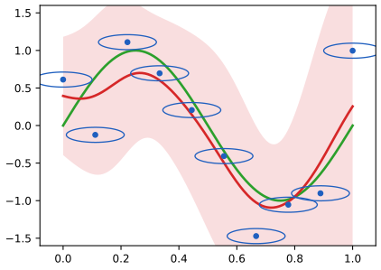
fig6_3. Download: PDF · SVGMore flexible components are possible, for instance different variances for \(\mathbf{x}\) and \(t\), or a Gaussian mixture fitted to \(p(t,\mathbf{x})\) by EM (Chapter 9; Ghahramani and Jordan, 1994) and then conditioned. The latter has fewer components than data points, so predictions are cheaper, but it is no longer a sum of kernels evaluated at the training points, and the cost has moved to training.
6.4 Gaussian processes
pp. 303–304 In Section 6.1 kernels arose from a non-probabilistic model. Here they arise in a Bayesian setting. The idea of a Gaussian process (GP) is to drop the parametric model \(y(\mathbf{x},\mathbf{w})\) and put a prior directly on the function \(y(\mathbf{x})\). This looks hard, since functions form an infinite-dimensional space, but only the function values at the training and test inputs ever matter, and those are a finite vector. A Gaussian process is a collection of random variables \(\{y(\mathbf{x}):\mathbf{x}\in\mathcal{X}\}\) such that every finite subcollection has a joint Gaussian distribution. Because a marginal of a Gaussian is Gaussian, the specifications for different finite sets are consistent with each other (the marginal of \(\N(\mathbf{0},\mathbf{K}_{N+1})\) over the first \(N\) variables is \(\N(\mathbf{0},\mathbf{K}_N)\), by the marginal formula in the toolkit), and the Kolmogorov extension theorem then gives a process on all of \(\mathcal{X}\).
The equivalents of GP regression have many names: kriging in geostatistics (Cressie, 1993); ARMA models, Kalman filters (Section 13.3) and RBF networks can all be viewed as Gaussian processes. Reviews: MacKay (1998), Williams (1999), Rasmussen and Williams (2006).
6.4.1 Linear regression revisited
pp. 304–306, (6.49)–(6.56) Start from a model one already knows: \(y(\mathbf{x})=\mathbf{w}^\T\bm\phi(\mathbf{x})\) with \(M\) fixed basis functions (6.49), and the prior
\[ p(\mathbf{w})=\N(\mathbf{w}\given\mathbf{0},\alpha^{-1}\mathbf{I}) \tag{6.50} \]with precision \(\alpha\). Each draw of \(\mathbf{w}\) is a function. At the training inputs the function values form the vector
\[ \mathbf{y}=\bm\Phi\mathbf{w}, \tag{6.51} \]with \(\bm\Phi_{nk}=\phi_k(\mathbf{x}_n)\). Since \(\mathbf{y}\) is a linear transformation of a Gaussian vector it is Gaussian (a linear map of a Gaussian: the characteristic function \(\E[e^{\mathrm{i}\mathbf{s}^\T\bm\Phi\mathbf{w}}]\)
Filling the gap 6.8: the prior over function values is \(\N(\mathbf{0},\alpha^{-1}\bm\Phi\bm\Phi^\T)\) p. 305, (6.52)–(6.54); Exercise 2.31
Derivation
By linearity of expectation and \(\E[\mathbf{w}]=\mathbf{0}\), \(\E[\mathbf{y}]=\bm\Phi\E[\mathbf{w}]=\mathbf{0}\) (6.52). Since the mean is zero, the covariance is the second moment, and \(\E[\mathbf{w}\mathbf{w}^\T]\)
whose entries are the inner products of feature vectors scaled by the prior variance,
\[ K_{nm}=k(\mathbf{x}_n,\mathbf{x}_m)=\frac1\alpha\bm\phi(\mathbf{x}_n)^\T\bm\phi(\mathbf{x}_m). \tag{6.54} \]The same computation for two arbitrary inputs gives \(\E[y(\mathbf{x})y(\mathbf{x}')]\)
In general, a stochastic process \(y(\mathbf{x})\) is specified by the joint distribution of any finite set of its values, in a consistent manner; for a Gaussian process the second-order statistics determine everything. With no prior knowledge of the mean we take it to be zero (by symmetry, as for the zero-mean weight prior), and the process is then specified by its covariance function, the kernel,
\[ \E[y(\mathbf{x}_n)y(\mathbf{x}_m)]=k(\mathbf{x}_n,\mathbf{x}_m). \tag{6.55} \](For two-dimensional inputs the process is also called a Gaussian random field.) The kernel can also be chosen directly. Figure 6.4 shows functions sampled from a GP with the Gaussian kernel (6.23) and with the exponential kernel
\[ k(x,x')=\exp(-\theta|x-x'|), \tag{6.56} \]the covariance of the Ornstein-Uhlenbeck process (Uhlenbeck and Ornstein, 1930).
Filling the gap 6.9: sampling a GP, and why the exponential kernel is the Ornstein-Uhlenbeck process pp. 305–306, Figure 6.4
Derivation
How a figure like 6.4 is drawn. Choose a grid \(x_1,\dots,x_N\), form \(\mathbf{K}\), and add a small jitter, \(\mathbf{K}+\epsilon\mathbf{I}\)
Ornstein-Uhlenbeck. The stochastic differential equation \(\d y=-\theta y\,\d s+\sqrt{2\theta}\,\d W_s\) has the stationary solution with \(\operatorname{var}[y]=\sigma_W^2/(2\theta)=1\) (setting \(\d\,\E[y^2]/\d s=-2\theta\E[y^2]+2\theta=0\)), and \(\E[y(s)y(s+\tau)]\)
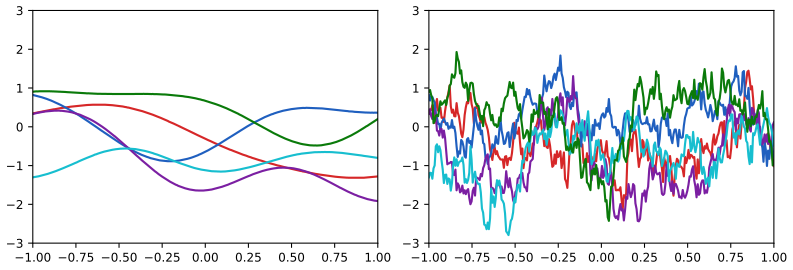
fig6_4. Download: PDF · SVG6.4.2 Gaussian processes for regression
pp. 306–311, (6.57)–(6.68) Observed targets contain noise, \(t_n=y_n+\epsilon_n\) (6.57), with \(\epsilon_n\) independent for each \(n\) and Gaussian,
\[ p(t_n\given y_n)=\N(t_n\given y_n,\beta^{-1}), \tag{6.58} \] \[ p(\mathbf{t}\given\mathbf{y})=\N(\mathbf{t}\given\mathbf{y},\beta^{-1}\mathbf{I}_N), \tag{6.59} \]and the GP prior supplies the marginal
\[ p(\mathbf{y})=\N(\mathbf{y}\given\mathbf{0},\mathbf{K}). \tag{6.60} \]The kernel is chosen so that nearby inputs have strongly correlated function values. Integrating out \(\mathbf{y}\) gives the distribution of the targets,
\[ p(\mathbf{t})=\int p(\mathbf{t}\given\mathbf{y})p(\mathbf{y})\,\d\mathbf{y}=\N(\mathbf{t}\given\mathbf{0},\mathbf{C}),\qquad C(\mathbf{x}_n,\mathbf{x}_m)=k(\mathbf{x}_n,\mathbf{x}_m)+\beta^{-1}\delta_{nm}. \tag{6.61, 6.62} \]This is the linear-Gaussian result (2.115) with the identity as the linear map (toolkit); it can also be seen directly, since \(\mathbf{t}=\mathbf{y}+\bm\epsilon\) is a sum of two independent Gaussian vectors with means \(\mathbf{0}\) and covariances \(\mathbf{K}\) and \(\beta^{-1}\mathbf{I}\), and covariances of independent summands add. A popular choice of kernel is the exponential of a quadratic form with constant and linear terms,
\[ k(\mathbf{x}_n,\mathbf{x}_m)=\theta_0\exp\!\Big\{-\frac{\theta_1}2\|\mathbf{x}_n-\mathbf{x}_m\|^2\Big\}+\theta_2+\theta_3\,\mathbf{x}_n^\T\mathbf{x}_m. \tag{6.63} \]It is valid: the first term is \(\theta_0\) times a Gaussian kernel, the second a constant kernel, the third a linear kernel, combined by (6.13) and (6.17). Here \(\theta_0\) is the signal variance, \(\theta_1=\ell^{-2}\) is the inverse squared length scale, \(\theta_2\) allows a constant offset (a random bias of variance \(\theta_2\)), and \(\theta_3\) a random linear trend, the parametric linear model. Figure 6.5 shows samples for several values; Figure 6.6 shows data points drawn from (6.60)–(6.61).
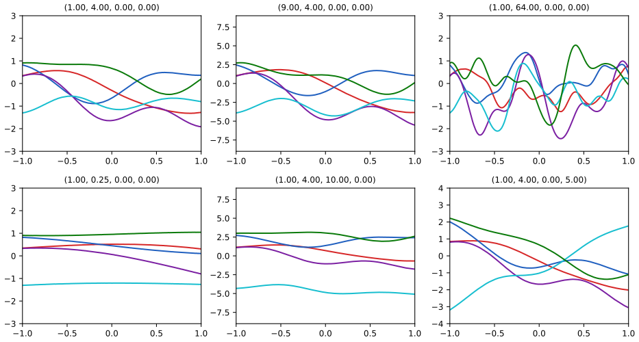
fig6_5. Download: PDF · SVG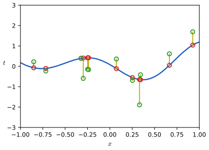
fig6_6. Download: PDF · SVGThe predictive distribution. Given the training targets \(\mathbf{t}_N=(t_1,\dots,t_N)^\T\) at \(\mathbf{x}_1,\dots,\mathbf{x}_N\), we want \(p(t_{N+1}\given\mathbf{t}_N)\) at a new input \(\mathbf{x}_{N+1}\) (inputs are suppressed in the notation). The joint distribution of the \(N+1\) targets is, by (6.61) applied to \(N+1\) points,
\[ p(\mathbf{t}_{N+1})=\N(\mathbf{t}_{N+1}\given\mathbf{0},\mathbf{C}_{N+1}),\qquad \mathbf{C}_{N+1}=\begin{pmatrix}\mathbf{C}_N&\mathbf{k}\\\mathbf{k}^\T&c\end{pmatrix}, \tag{6.64, 6.65} \]where \(\mathbf{C}_N\) has entries (6.62), \(\mathbf{k}\) has entries \(k(\mathbf{x}_n,\mathbf{x}_{N+1})\), and \(c\)
Result 6.4 (predictive distribution of Gaussian process regression) p. 307, (6.66), (6.67); Exercise 6.20
The conditional distribution \(p(t_{N+1}\given\mathbf{t})\) is Gaussian with
\[ m(\mathbf{x}_{N+1})=\mathbf{k}^\T\mathbf{C}_N^{-1}\mathbf{t}, \tag{6.66} \] \[ \sigma^2(\mathbf{x}_{N+1})=c-\mathbf{k}^\T\mathbf{C}_N^{-1}\mathbf{k}. \tag{6.67} \]Both depend on the test input through \(\mathbf{k}\) (and \(c\)). The variance does not depend on the observed targets. The variance of the underlying function value \(y_{N+1}\) (without the observation noise) is \(\sigma^2-\beta^{-1}\)
Proof (two ways)
(a) From the conditional Gaussian formulas. For a zero-mean Gaussian vector \((\mathbf{x}_a,\mathbf{x}_b)\) with covariance blocks \(\bm\Sigma_{aa},\bm\Sigma_{ab},\bm\Sigma_{bb}\), the conditional is \(\N(\mathbf{x}_a\given\bm\Sigma_{ab}\bm\Sigma_{bb}^{-1}\mathbf{x}_b,\;\bm\Sigma_{aa}-\bm\Sigma_{ab}\bm\Sigma_{bb}^{-1}\bm\Sigma_{ba})\) (eqs (2.81), (2.82), proved in the toolkit). Take \(\mathbf{x}_a=t_{N+1}\), \(\mathbf{x}_b=\mathbf{t}\): \(\bm\Sigma_{aa}=c\), \(\bm\Sigma_{ab}=\mathbf{k}^\T\), \(\bm\Sigma_{bb}=\mathbf{C}_N\). This gives (6.66) and (6.67) at once. (The official solution orders the blocks the other way, with \(t_{N+1}\) first; the result is the same.)
(b) By completing the square. Let \(s\)
As a function of \(\tau=t_{N+1}\) (with \(\mathbf{t}\) fixed) the exponent of the joint density is \(-\frac12(\mathbf{t}^\T,\tau)\mathbf{C}_{N+1}^{-1}(\mathbf{t}^\T,\tau)^\T\)
The variance bound. \(\mathbf{C}_{N+1}\) is positive definite, hence so is its Schur complement \(c-\mathbf{k}^\T\mathbf{C}_N^{-1}\mathbf{k}>0\). Since \(\mathbf{k}^\T\mathbf{C}_N^{-1}\mathbf{k}\) is the variance of the part of the new function value explained by the data (a squared norm, \(\ge0\)), \(\sigma^2\le c\) (never worse than the prior), and \(\sigma^2-\beta^{-1}\) is a conditional variance of \(y_{N+1}\) (a Gaussian conditional covariance, \(\ge0\)).∎
Validity of the covariance. The only requirement on the kernel is that \(\mathbf{C}\) be positive definite. If \(\lambda_i\) are the eigenvalues of \(\mathbf{K}\) then those of \(\mathbf{C}=\mathbf{K}+\beta^{-1}\mathbf{I}\) are \(\lambda_i+\beta^{-1}\) (same eigenvectors), so a PSD Gram matrix (Section 6.2) suffices: a zero eigenvalue of \(\mathbf{K}\) still gives a positive eigenvalue of \(\mathbf{C}\) because \(\beta>0\). All the constructions of Section 6.2 can be used.
The mean is a kernel expansion. With \(a_n\) the \(n\)-th component of \(\mathbf{C}_N^{-1}\mathbf{t}\),
\[ m(\mathbf{x}_{N+1})=\sum_{n=1}^{N}a_n\,k(\mathbf{x}_n,\mathbf{x}_{N+1}), \tag{6.68} \]so for a kernel depending on \(\|\mathbf{x}_n-\mathbf{x}_m\|\) only, this is an expansion in radial basis functions, one per data point. Compare (6.66) with (6.9): they are the same formula with \(\lambda=\beta^{-1}\). The posterior mean of a GP is kernel ridge regression with regularisation parameter equal to the noise variance; the GP adds the predictive variance (6.67). In Figure 6.8 the shaded band is \(\pm2\sigma\).
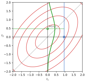
fig6_7. Download: PDF · SVG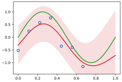
fig6_8. Download: PDF · SVGFilling the gap 6.10: a GP with a finite-basis kernel is Bayesian linear regression p. 309; Exercise 6.21
The book says that for a kernel defined by finitely many basis functions one recovers the Bayesian linear regression predictive distribution (3.58) of Section 3.3.2. Both distributions are Gaussian, so it suffices to match mean and variance. The tools are the push-through identity of Gap 6.1 and the Woodbury identity (toolkit).
Derivation
Take \(k(\mathbf{x},\mathbf{x}')\)
Mean. By push-through (matrix identity (C.6) of the book), \(\bm\Phi^\T(\alpha^{-1}\bm\Phi\bm\Phi^\T+\beta^{-1}\mathbf{I}_N)^{-1}\)
Variance. Expanding (6.67),
\[ \sigma^2=\alpha^{-1}\bm\phi^\T\bm\phi+\beta^{-1}-\alpha^{-2}\bm\phi^\T\bm\Phi^\T\mathbf{C}_N^{-1}\bm\Phi\bm\phi=\beta^{-1}+\bm\phi^\T\Big[\alpha^{-1}\mathbf{I}-\alpha^{-2}\bm\Phi^\T(\alpha^{-1}\bm\Phi\bm\Phi^\T+\beta^{-1}\mathbf{I}_N)^{-1}\bm\Phi\Big]\bm\phi. \]The Woodbury identity \((\mathbf{A}+\mathbf{U}\mathbf{B}\mathbf{V})^{-1}\)
which is (3.59). The parameter-space and function-space views give the same predictive distribution.∎
Filling the gap 6.11: computational cost, and several test points pp. 309–311; Exercises 6.22, 6.23
Derivation
Cost. The central operation is solving with the \(N\times N\) matrix \(\mathbf{C}_N\), \(O(N^3)\) by Cholesky \(\mathbf{C}_N=\mathbf{L}\mathbf{L}^\T\) (\(N^3/6\) multiplications), done once per training set and set of hyperparameters; the basis function model inverts the \(M\times M\) matrix \(\mathbf{S}_N^{-1}\), \(O(M^3)\). Afterwards, for each test point the mean (6.66) costs \(O(N)\) given \(\mathbf{a}=\mathbf{C}_N^{-1}\mathbf{t}\) (one dot product), and the variance (6.67) costs \(O(N^2)\) because \(\mathbf{k}^\T\mathbf{C}_N^{-1}\mathbf{k}\) \(L\) test points at once (Exercise 6.22). Let \(\mathbf{K}_*\) be the \(N\times L\) matrix with entries \(k(\mathbf{x}_n,\mathbf{x}_{N+l})\) and \(\mathbf{K}_{**}\) the \(L\times L\) kernel matrix of the test inputs. The joint of training and test targets is Gaussian with covariance
\[ \begin{pmatrix}\mathbf{C}_N&\mathbf{K}_*\\\mathbf{K}_*^\T&\mathbf{K}_{**}+\beta^{-1}\mathbf{I}_L\end{pmatrix}, \]
so by the same conditional formulas The marginal for the single test target \(t_j\), \(N+1\le j\le N+L\), keeps the \(j\)-th entry of the mean, \(\mathbf{k}_j^\T\mathbf{C}_N^{-1}\mathbf{t}\), and the \(j\)-th diagonal entry of the covariance, \(k(\mathbf{x}_j,\mathbf{x}_j)+\beta^{-1}\) Several targets (Exercise 6.23). If the \(D\) components of \(\mathbf{t}\) are independent given the input, with the same kernel, then with \(\mathbf{T}\) the \(N\times D\) matrix of training targets (rows \(\mathbf{t}_n^\T\)), \(p(\mathbf{t}_{N+1}\given\mathbf{T})\)
Kernels for inputs on a circle or a sphere
Sometimes the inputs live on a sphere \(S^{D-1}=\{\mathbf{x}:\|\mathbf{x}\|=1\}\) (directions, geographic positions) or a circle (angles, time of day). The rules of Section 6.2 give valid kernels there, and a tempting construction fails.
Filling the gap 6.12: valid and invalid kernels on the circle and the sphere extension of Section 6.2, (6.19), (6.16)
Derivation
Restriction. If \(k\) is a valid kernel on \(\R^D\), its restriction to the sphere is valid: Gram matrices of the restriction are Gram matrices of \(k\) at points that happen to lie on the sphere (or (6.19) with the inclusion map as \(\bm\phi\)).
Zonal kernels. For unit vectors, \(\|\mathbf{x}-\mathbf{x}'\|^2\)
a function of the cosine of the angle only (a zonal kernel, invariant under rotations of the sphere), valid by (6.16) applied to the linear kernel and (6.13). It uses the chordal distance. On the circle, with \(\mathbf{x}=(\cos\vartheta,\sin\vartheta)\) and \(\|\mathbf{x}-\mathbf{x}'\|^2\)
The geodesic Gaussian is not valid. Replacing the chordal distance by the geodesic (angular) distance \(d_g\), \(k=\exp(-d_g^2/2\sigma^2)\), looks natural but is not positive semidefinite in general: for 12 equally spaced points on the circle I computed the smallest Gram eigenvalue as \(-0.005\) for \(\sigma=1\) and \(-0.237\) for \(\sigma=2\) (for the chordal version all eigenvalues are positive). The geodesic distance on a circle is not a Euclidean distance (it is not the norm of a difference of an embedding), so (6.19) does not apply, and the Fourier coefficients of this function on the circle are not all non-negative (Schoenberg, 1942).
Characterisation (stated, not proved). A continuous function of the form \(k(\mathbf{x},\mathbf{x}')\)
6.4.3 Learning the hyperparameters
pp. 311–312, (6.69), (6.70) Predictions depend on the covariance function, so rather than fixing it we use a parametric family and infer its parameters \(\bm\theta\) (length scales, signal and noise variances, ...), the hyperparameters of the GP. The simplest approach maximises the likelihood \(p(\mathbf{t}\given\bm\theta)\), the analogue of the type-2 maximum likelihood (evidence approximation) of Section 3.5. Because \(\mathbf{t}\sim\N(\mathbf{0},\mathbf{C}_N)\) by (6.61), the log likelihood is just the log of a Gaussian density:
\[ \ln p(\mathbf{t}\given\bm\theta)=-\frac12\ln|\mathbf{C}_N|-\frac12\mathbf{t}^\T\mathbf{C}_N^{-1}\mathbf{t}-\frac N2\ln(2\pi). \tag{6.69} \]The first term penalises complexity (a large determinant means a broad, flexible prior over \(\mathbf{t}\)), the second measures fit; the balance is automatic (Occam's razor), with no cross-validation. With the finite basis kernel (6.54), (6.69) equals the log evidence (3.86) (matrix determinant lemma \(|\beta^{-1}\mathbf{I}_N\)
Filling the gap 6.13: the gradient of the log marginal likelihood p. 311, (6.70); book Appendix C, (C.21), (C.22)
Derivation
Two matrix-calculus facts (toolkit), for a symmetric positive definite \(\mathbf{C}(\theta)\) depending on a scalar \(\theta\), with \(\mathbf{C}'=\partial\mathbf{C}/\partial\theta\):
- (C.21) \(\dfrac{\partial\mathbf{C}^{-1}}{\partial\theta}\)
\({}=-\mathbf{C}^{-1}\mathbf{C}'\mathbf{C}^{-1}\): differentiate \(\mathbf{C}\mathbf{C}^{-1}=\mathbf{I}\) to get \(\mathbf{C}'\mathbf{C}^{-1}\) \({}+\mathbf{C}(\mathbf{C}^{-1})'\) \({}=\mathbf{0}\). - (C.22) \(\dfrac{\partial\ln|\mathbf{C}|}{\partial\theta}\)
\({}=\Tr(\mathbf{C}^{-1}\mathbf{C}')\): for an eigen-decomposition \(\ln|\mathbf{C}|=\sum_i\ln\lambda_i\), and the first-order change of the determinant is \(\d|\mathbf{C}|\) \({}=|\mathbf{C}|\Tr(\mathbf{C}^{-1}\d\mathbf{C})\) (Jacobi's formula).
Apply them to (6.69), term by term; the constant has zero derivative:
\[ \frac{\partial}{\partial\theta_i}\Big[-\tfrac12\ln|\mathbf{C}_N|\Big]=-\tfrac12\Tr\Big(\mathbf{C}_N^{-1}\frac{\partial\mathbf{C}_N}{\partial\theta_i}\Big),\qquad \frac{\partial}{\partial\theta_i}\Big[-\tfrac12\mathbf{t}^\T\mathbf{C}_N^{-1}\mathbf{t}\Big]=+\tfrac12\mathbf{t}^\T\mathbf{C}_N^{-1}\frac{\partial\mathbf{C}_N}{\partial\theta_i}\mathbf{C}_N^{-1}\mathbf{t}. \]Adding,
\[ \frac{\partial}{\partial\theta_i}\ln p(\mathbf{t}\given\bm\theta)=-\frac12\Tr\Big(\mathbf{C}_N^{-1}\frac{\partial\mathbf{C}_N}{\partial\theta_i}\Big)+\frac12\mathbf{t}^\T\mathbf{C}_N^{-1}\frac{\partial\mathbf{C}_N}{\partial\theta_i}\mathbf{C}_N^{-1}\mathbf{t}. \tag{6.70} \]With \(\mathbf{a}=\mathbf{C}_N^{-1}\mathbf{t}\) this is \(\frac12\Tr\{(\mathbf{a}\mathbf{a}^\T-\mathbf{C}_N^{-1})\,\partial\mathbf{C}_N/\partial\theta_i\}\), which is how it is coded: one Cholesky factorisation gives \(\mathbf{a}\) and \(\mathbf{C}_N^{-1}\) (\(O(N^3)\)), and each hyperparameter then needs only the elementwise product of \(\mathbf{a}\mathbf{a}^\T-\mathbf{C}_N^{-1}\) with \(\partial\mathbf{C}_N/\partial\theta_i\) summed, \(O(N^2)\).
Derivatives for the kernel (6.63). With \(\Delta_{nm}=\|\mathbf{x}_n-\mathbf{x}_m\|^2\) and \(e_{nm}=\exp(-\theta_1\Delta_{nm}/2)\): \(\partial C_{nm}/\partial\theta_0=e_{nm}\); \(\partial C_{nm}/\partial\theta_1\)
The log likelihood is generally not concave, so there can be several local maxima (for example "short length scale, small noise" versus "long length scale, large noise"); restarts help. It is easy to add a prior over \(\bm\theta\) and maximise the log posterior (then add \(\partial\ln p(\bm\theta)/\partial\theta_i\) to (6.70)). A fully Bayesian treatment would integrate over \(\bm\theta\), which is intractable and needs approximation (MCMC, Chapter 11). The model assumed that the noise variance \(\beta^{-1}\) is constant; for heteroscedastic problems a second GP can represent \(\ln\beta(\mathbf{x})\), the logarithm because a precision is positive (Goldberg et al., 1998).
6.4.4 Automatic relevance determination
pp. 312–313, (6.71), (6.72) Give each input dimension its own precision parameter \(\eta_i\). For \(\mathbf{x}=(x_1,x_2)\),
\[ k(\mathbf{x},\mathbf{x}')=\theta_0\exp\Big\{-\frac12\sum_{i=1}^{2}\eta_i(x_i-x_i')^2\Big\}. \tag{6.71} \]This is a product over dimensions of Gaussian kernels with length scales \(\ell_i=\eta_i^{-1/2}\), valid by (6.22) and (6.13). When \(\eta_i\) is small the function varies slowly in the direction \(x_i\); in the limit \(\eta_i\to0\) the kernel (hence every sample function) does not depend on \(x_i\) at all (Figure 6.9). Maximising the marginal likelihood over the \(\eta_i\) (the gradient (6.70) with \(\partial C_{nm}/\partial\eta_i\)
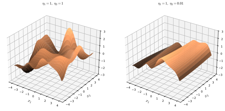
fig6_9. Download: PDF · SVGFilling the gap 6.14: why maximum likelihood switches irrelevant inputs off p. 312
The book asserts that adapting the \(\eta_i\) by maximum likelihood reveals unimportant inputs. This is the Occam argument made concrete.
Derivation
Let \(x_2\) carry no information about \(t\). Compare the models with \(\eta_2=0\) (the kernel ignores \(x_2\)) and \(\eta_2>0\). Raising \(\eta_2\) from zero decreases the off-diagonal covariances \(k(\mathbf{x}_n,\mathbf{x}_m)\) between points that differ in \(x_2\) (the multiplier \(e^{-\eta_2(x_{n2}-x_{m2})^2/2}\) is \(<1\)), so the matrix \(\mathbf{K}\) moves towards \(\theta_0\mathbf{I}\) and the determinant \(|\mathbf{C}_N|\) increases (for fixed diagonal \(\theta_0+\beta^{-1}\), the determinant is largest when the matrix is diagonal, by Hadamard's inequality). The prior then spreads its mass over more possible data sets, so the data-fit term can only gain if the data actually have structure along \(x_2\). If they do not, the data-fit term does not improve and the complexity term \(-\frac12\ln|\mathbf{C}_N|\) falls, and the gradient (6.70) is typically negative at \(\eta_2=0^+\): \(\eta_2\) runs towards zero. If \(x_2\) is informative, the data-fit term gains more than the complexity term loses, and \(\eta_2\) stays positive. This is the same mechanism by which the evidence approximation drives the precision of an unneeded weight to infinity (Section 3.5, Section 7.2.2).
(Hadamard's inequality is used only for intuition; the decrease of \(\ln|\mathbf{C}_N|\) as dimensions are switched off is not guaranteed for every data configuration, which is one reason ARD can also fail with little data.)∎
ARD is illustrated (Nabney, 2002) on a synthetic data set with three inputs (Figure 6.10): \(t\) is generated from a function of \(x_1\) (\(\sin(2\pi x_1)\) plus Gaussian noise), \(x_2\) is a noisy copy of \(x_1\), and \(x_3\) is independent noise. Maximising the marginal likelihood with scaled conjugate gradients, \(\eta_1\) converges to a relatively large value, \(\eta_2\) to a much smaller one and \(\eta_3\) to a very small value, indicating that \(x_3\) is irrelevant. The ARD idea is easily built into (6.63):
\[ k(\mathbf{x}_n,\mathbf{x}_m)=\theta_0\exp\Big\{-\frac12\sum_{i=1}^{D}\eta_i(x_{ni}-x_{mi})^2\Big\}+\theta_2+\theta_3\sum_{i=1}^{D}x_{ni}x_{mi}, \tag{6.72} \]which has been found useful for a range of regression problems.
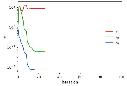
fig6_10. Download: PDF · SVG6.4.5 Gaussian processes for classification
pp. 313–315, (6.73)–(6.76) A GP produces values on the whole real line, but class probabilities must lie in \((0,1)\). As in logistic regression, put the GP on an activation function \(a(\mathbf{x})\) and squash it with the logistic sigmoid \(y=\sigma(a)\) (4.59). For two classes, \(t\in\{0,1\}\), the Bernoulli likelihood is
\[ p(t\given a)=\sigma(a)^t\big(1-\sigma(a)\big)^{1-t}. \tag{6.73} \]A sample from a GP over \(a(\mathbf{x})\), transformed pointwise, is a non-Gaussian random function with values in \((0,1)\) (Figure 6.11).
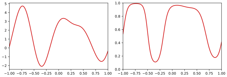
fig6_11. Download: PDF · SVGLet the training inputs be \(\mathbf{x}_1,\dots,\mathbf{x}_N\) with labels \(\mathbf{t}_N=(t_1,\dots,t_N)^\T\) and a test point \(\mathbf{x}_{N+1}\). Put the GP prior on the vector \(\mathbf{a}_{N+1}\)
There is no noise term of the regression type, because the labels are assumed correctly assigned (the Bernoulli likelihood already contains the randomness). The small constant \(\nu\), typically fixed in advance (for instance \(10^{-6}\) up to \(10^{-2}\)), only keeps \(\mathbf{C}\) positive definite numerically; a larger \(\nu\) adds a small independent component to the latent function. The kernel \(k\) is any PSD kernel with parameters \(\bm\theta\). For two classes it suffices to predict
\[ p(t_{N+1}=1\given\mathbf{t}_N)=\int p(t_{N+1}=1\given a_{N+1})\,p(a_{N+1}\given\mathbf{t}_N)\,\d a_{N+1},\qquad p(t_{N+1}=1\given a_{N+1})=\sigma(a_{N+1}). \tag{6.76} \]This integral is intractable. It can be approximated by sampling (Neal, 1997), or analytically if one has a Gaussian approximation to the posterior \(p(a_{N+1}\given\mathbf{t}_N)\), because the convolution of a sigmoid with a Gaussian has the approximation (4.153). The usual justification for a Gaussian posterior (central limit theorem) does not apply directly, since the number of variables grows with the data; but if the number of points in a fixed region increases, the uncertainty in \(a(\mathbf{x})\) there shrinks and the posterior tends to a Gaussian (Williams and Barber, 1998). Three approaches have been used: the local variational bound (10.144) of Section 10.6 (Gibbs and MacKay, 2000; extended to \(K>2\) by Gibbs, 1997), expectation propagation (Section 10.7; Opper and Winther, 2000; Minka, 2001; Seeger, 2003), which works well because the true posterior is unimodal, and the Laplace approximation, treated next.
6.4.6 Laplace approximation
pp. 315–319, (6.77)–(6.94) The Laplace approximation (Section 4.4) replaces a posterior by a Gaussian centred at its mode with covariance the inverse of the negative Hessian of the log density there. We need it for \(p(a_{N+1}\given\mathbf{t}_N)\). The route is: marginalise \(\mathbf{a}_N\) in two steps, first approximating \(p(\mathbf{a}_N\given\mathbf{t}_N)\), then using the GP conditional for the test point.
Filling the gap 6.15: reducing the test posterior to a posterior over the training activations pp. 315–316, (6.77), (6.78)
Derivation
By the sum rule and Bayes' theorem,
\[ p(a_{N+1}\given\mathbf{t}_N)=\int p(a_{N+1},\mathbf{a}_N\given\mathbf{t}_N)\,\d\mathbf{a}_N=\frac1{p(\mathbf{t}_N)}\int p(a_{N+1},\mathbf{a}_N)\,p(\mathbf{t}_N\given a_{N+1},\mathbf{a}_N)\,\d\mathbf{a}_N. \]The labels depend on the activations only at their own inputs, so \(p(\mathbf{t}_N\given a_{N+1},\mathbf{a}_N)\)
The first factor is the GP conditional of the prior (6.74) (the same conditional as in regression, Result 6.4, with no observation noise on \(\mathbf{a}_N\), only the jitter \(\nu\) inside \(\mathbf{C}\)),
\[ p(a_{N+1}\given\mathbf{a}_N)=\N\big(a_{N+1}\given\mathbf{k}^\T\mathbf{C}_N^{-1}\mathbf{a}_N,\;c-\mathbf{k}^\T\mathbf{C}_N^{-1}\mathbf{k}\big), \tag{6.78} \]with \(c=k(\mathbf{x}_{N+1},\mathbf{x}_{N+1})+\nu\). So the unknown quantity is \(p(\mathbf{a}_N\given\mathbf{t}_N)\); it is the only place where the non-Gaussian likelihood enters, and a Gaussian approximation to it turns (6.77) into a convolution of two Gaussians.∎
The prior is \(p(\mathbf{a}_N)\)
Taylor-expand the log posterior up to a constant,
\[ \Psi(\mathbf{a}_N)=\ln p(\mathbf{a}_N)+\ln p(\mathbf{t}_N\given\mathbf{a}_N)=-\frac12\mathbf{a}_N^\T\mathbf{C}_N^{-1}\mathbf{a}_N-\frac N2\ln(2\pi)-\frac12\ln|\mathbf{C}_N|+\mathbf{t}_N^\T\mathbf{a}_N-\sum_{n=1}^{N}\ln(1+e^{a_n}). \tag{6.80} \]Erratum. The book prints "+const" at the end of (6.80); it should be omitted, since the right side is already the exact sum \(\ln p(\mathbf{a}_N)\)
Filling the gap 6.16: gradient, Hessian and uniqueness of the mode pp. 316–317, (6.81), (6.82); Exercise 6.24
Derivation
Gradient. \(\partial\ln(1+e^{a})/\partial a\)
Hessian. By (4.88), \(\sigma'(a)=\sigma(a)(1-\sigma(a))\). Differentiating (6.81) again, \(\partial\sigma_n/\partial a_m\)
Positive definiteness (Exercise 6.24). A diagonal matrix with positive entries is PD: \(\mathbf{v}^\T\mathbf{W}\mathbf{v}\)
Consequences. \(\Psi\) is strictly concave, so the posterior is log-concave. It has at most one stationary point, which is the global maximum. A maximum exists because \(\Psi(\mathbf{a})\to-\infty\) as \(\|\mathbf{a}\|\to\infty\): the term \(-\frac12\mathbf{a}^\T\mathbf{C}^{-1}\mathbf{a}\) decreases quadratically, while the remaining terms \(\mathbf{t}^\T\mathbf{a}-\sum\ln(1+e^{a_n})\) are bounded above by \(0\). So the posterior is unimodal, which makes the Laplace approximation reasonable, and Newton's method converges to the mode. The posterior is not Gaussian, because the Hessian depends on \(\mathbf{a}_N\) through \(\mathbf{W}_N\).∎
Filling the gap 6.17: finding the mode by Newton-Raphson (IRLS) p. 317, (6.83), (6.84); Exercise 6.25
Derivation
The Newton-Raphson update (4.92) for maximising \(\Psi\) is \(\mathbf{a}^{\rm new}\)
Now \((\mathbf{C}^{-1}+\mathbf{W})\mathbf{C}\)
This is iteratively reweighted least squares (Section 4.3.3): at each step a weighted "working response" \(\mathbf{W}^{-1}(\mathbf{t}-\bm\sigma)+\mathbf{a}\) is smoothed by the GP. The form with \(\mathbf{C}(\mathbf{I}+\mathbf{W}\mathbf{C})^{-1}\) needs only \(\mathbf{C}\) (never \(\mathbf{C}^{-1}\)). A numerically stable implementation uses \(\mathbf{B}\)
At convergence the gradient vanishes: \(\mathbf{t}_N-\bm\sigma_N\)
This is an implicit equation for \(\mathbf{a}^\star\) (since \(\bm\sigma_N\) depends on it), and says that the mode is a kernel expansion with coefficients \(t_n-\sigma(a_n^\star)\), the residual of each training label: well-classified points have small coefficients and contribute little. Newton's method on a strictly concave function with a Lipschitz Hessian converges (quadratically near the optimum); in practice 5 to 10 iterations are enough.∎
At the mode we evaluate the Hessian, with \(\mathbf{W}_N\) computed from \(\mathbf{a}_N^\star\),
\[ \mathbf{H}=-\nabla\nabla\Psi(\mathbf{a}_N^\star)=\mathbf{W}_N+\mathbf{C}_N^{-1}, \tag{6.85} \]which defines the Gaussian approximation to the posterior,
\[ q(\mathbf{a}_N)=\N\big(\mathbf{a}_N\given\mathbf{a}_N^\star,\mathbf{H}^{-1}\big). \tag{6.86} \]By Woodbury, \(\mathbf{H}^{-1}\)
Filling the gap 6.18: the predictive distribution of the activation p. 317, (6.87), (6.88); Exercise 6.26
Derivation
Replace \(p(\mathbf{a}_N\given\mathbf{t}_N)\) in (6.77) by \(q(\mathbf{a}_N)\). Then \(a_{N+1}\) is the output of a linear-Gaussian model: given \(\mathbf{a}_N\), (6.78) says \(a_{N+1}\sim\N(\mathbf{A}\mathbf{a}_N,\,s_0)\) with \(\mathbf{A}=\mathbf{k}^\T\mathbf{C}_N^{-1}\) (a row vector) and \(s_0=c-\mathbf{k}^\T\mathbf{C}_N^{-1}\mathbf{k}\). The marginal formula (2.115) (toolkit) for \(\mathbf{x}\sim\N(\bm\mu,\bm\Lambda^{-1})\), \(\mathbf{y}\given\mathbf{x}\)
Mean. \(\mathbf{k}^\T\mathbf{C}_N^{-1}\mathbf{a}_N^\star\)
Variance. \(\var[a_{N+1}\given\mathbf{t}_N]\)
Compare with the regression variance (6.67): classification replaces the noise covariance \(\beta^{-1}\mathbf{I}\) by \(\mathbf{W}^{-1}\), a data-dependent diagonal "noise" which is large where the sigmoid is flat (\(W_{nn}\) small, points far from the boundary say little about \(a\)). Finally, with mean \(\mu\) and variance \(s^2\) the sigmoid-Gaussian convolution (4.153) gives
\[ p(t_{N+1}=1\given\mathbf{t}_N)\simeq\sigma\big(\kappa(s^2)\,\mu\big),\qquad\kappa(s^2)=\big(1+\pi s^2/8\big)^{-1/2}. \]The variance pulls the probability towards \(\frac12\) where the model is uncertain; because \(\kappa>0\), the decision boundary \(p=\frac12\) is where \(\mu=\mathbf{k}^\T(\mathbf{t}-\bm\sigma)=0\), independent of the variance, exactly as for Bayesian logistic regression (Section 4.5.2).∎
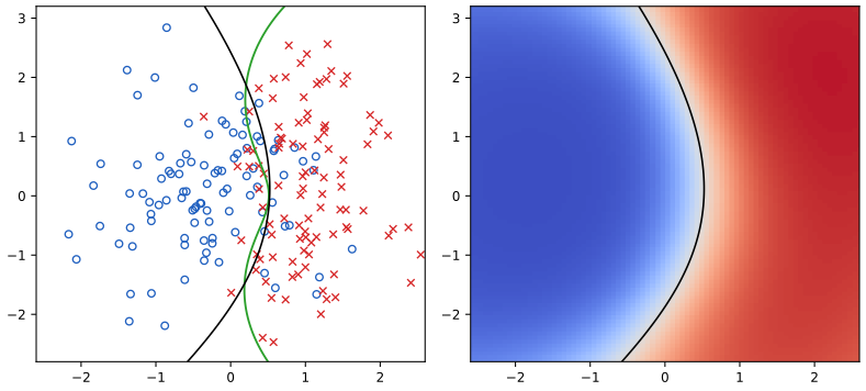
fig6_12. Download: PDF · SVGLearning the covariance parameters
pp. 317–318, (6.89)–(6.94) The kernel parameters \(\bm\theta\) are found by maximising the likelihood, with a penalty if desired,
\[ p(\mathbf{t}_N\given\bm\theta)=\int p(\mathbf{t}_N\given\mathbf{a}_N)\,p(\mathbf{a}_N\given\bm\theta)\,\d\mathbf{a}_N. \tag{6.89} \]Filling the gap 6.19: the Laplace approximation of the evidence p. 317, (6.89), (6.90); Exercise 6.27
Derivation
The integrand of (6.89) is \(e^{\Psi(\mathbf{a}_N)}\) (it is \(p(\mathbf{a}_N)p(\mathbf{t}_N\given\mathbf{a}_N)\) exactly, which is why the erratum to (6.80) removes "+const"). Around the mode, \(\Psi(\mathbf{a})\)
with \(\Psi(\mathbf{a}^\star)\)
The first three terms are the penalised log likelihood at the mode, the last is the Occam factor.∎
Filling the gap 6.20: the gradient of the approximate evidence with respect to the hyperparameters pp. 318, (6.91)–(6.94); Exercise 6.27
Changing \(\theta_j\) changes \(\mathbf{C}_N\) explicitly and also moves the mode \(\mathbf{a}^\star\) (and so \(\mathbf{W}\)). The book separates the two contributions. I checked the final formula against finite differences of (6.90) (random data, 7 points, three hyperparameters, with the mode found to machine precision) and it agrees to about 9 digits, after correcting two printing slips in the order of factors (flagged below).
Derivation
Write \(\mathbf{C}'\)
Step 1: no contribution of \(\mathbf{a}^\star\) through \(\Psi\). By the chain rule \(\frac{\d}{\d\theta_j}\Psi(\mathbf{a}^\star;\bm\theta)\)
Step 2: explicit dependence of the two terms on \(\mathbf{C}\). Holding \(\mathbf{a}\) and \(\mathbf{W}\) fixed, \(\Psi\) depends on \(\theta_j\) through \(-\frac12\mathbf{a}^\T\mathbf{C}^{-1}\mathbf{a}\)
Since \(\mathbf{W}+\mathbf{C}^{-1}\)
So the explicit part is
\[ \frac{\partial\ln p(\mathbf{t}_N\given\bm\theta)}{\partial\theta_j}\Big|_{\rm explicit}=\frac12\mathbf{a}^{\star\T}\mathbf{C}_N^{-1}\frac{\partial\mathbf{C}_N}{\partial\theta_j}\mathbf{C}_N^{-1}\mathbf{a}^\star-\frac12\Tr\Big\{(\mathbf{I}+\mathbf{W}_N\mathbf{C}_N)^{-1}\mathbf{W}_N\frac{\partial\mathbf{C}_N}{\partial\theta_j}\Big\}. \tag{6.91} \]Erratum-type note. The printed (6.91) has the factor \((\mathbf{I}+\mathbf{C}_N\mathbf{W}_N)^{-1}\mathbf{W}_N\); the correct one is \((\mathbf{I}+\mathbf{W}_N\mathbf{C}_N)^{-1}\mathbf{W}_N\) (the symmetric matrix \(\mathbf{W}^{1/2}(\mathbf{I}+\mathbf{W}^{1/2}\mathbf{C}\mathbf{W}^{1/2})^{-1}\mathbf{W}^{1/2}\)). The two give the same trace when \(\mathbf{C}'=\mathbf{I}\) (the jitter or noise parameter), by cyclicity of the trace and the push-through identity, but not in general; this slip is not on the official errata list, and finite differences confirm the version above.
Step 3: dependence through the mode. Only \(-\frac12\ln|\mathbf{W}+\mathbf{C}^{-1}|\) still depends on \(\mathbf{a}^\star\), through \(\mathbf{W}\)
so by the chain rule the contribution is
\[ -\frac12\sum_{n=1}^{N}\frac{\partial\ln|\mathbf{W}_N+\mathbf{C}_N^{-1}|}{\partial a^\star_n}\frac{\partial a^\star_n}{\partial\theta_j}=-\frac12\sum_{n=1}^{N}\big[(\mathbf{I}+\mathbf{C}_N\mathbf{W}_N)^{-1}\mathbf{C}_N\big]_{nn}\,\sigma_n^\star(1-\sigma_n^\star)(1-2\sigma_n^\star)\,\frac{\partial a_n^\star}{\partial\theta_j}. \tag{6.92} \]To get \(\partial\mathbf{a}^\star/\partial\theta_j\), differentiate the fixed-point condition \(\mathbf{a}^\star\)
Moving the last term to the left, \((\mathbf{I}+\mathbf{C}_N\mathbf{W}_N)\,\partial\mathbf{a}^\star/\partial\theta_j\)
The printed (6.94) writes \((\mathbf{I}+\mathbf{W}_N\mathbf{C}_N)^{-1}\); (6.93) as printed leads to \((\mathbf{I}+\mathbf{C}_N\mathbf{W}_N)^{-1}\), which is what finite differences confirm (this slip is also not on the official list).
The total gradient is the sum of (6.91) and (6.92), with (6.94) inserted into (6.92). Using \(\mathbf{C}^{-1}\mathbf{a}^\star\)
Extension to \(K>2\) classes uses the softmax in place of the sigmoid (Williams and Barber, 1998). Figure 6.12 uses a synthetic two-class problem (Appendix A of the book).
6.4.7 Connection to neural networks
pp. 319–320 For a Bayesian neural network, a prior over the weights \(\mathbf{w}\) together with the network function induces a prior over functions. In the framework of maximum likelihood the number of hidden units \(M\) must be limited to avoid over-fitting, but from a Bayesian viewpoint there is no reason to restrict the number of parameters according to the size of the data set. Neal (1996) showed that for a broad class of priors the distribution over functions tends to a Gaussian process as \(M\to\infty\). The argument is the central limit theorem.
Result 6.5 (infinitely wide networks are Gaussian processes: Neal's argument) p. 319; Neal (1996), Williams (1998)
Consider a network with \(M\) hidden units and one output
\[ f_M(\mathbf{x})=b+\sum_{j=1}^{M}v_j\,h(\mathbf{x};\mathbf{u}_j), \]with all parameters independent: \(b\sim\N(0,\sigma_b^2)\); the hidden-unit parameters \(\mathbf{u}_j\) (input weights and bias) i.i.d. from a distribution \(p(\mathbf{u})\); and output weights \(v_j\) i.i.d. with mean \(0\) and variance \(\sigma_v^2/M\). Suppose \(\E_{\mathbf{u}}[h(\mathbf{x};\mathbf{u})^2]<\infty\) for every \(\mathbf{x}\) (true, for example, for bounded activation functions such as tanh, logistic or erf). Then, for any finite set of inputs \(\mathbf{x}_1,\dots,\mathbf{x}_N\), as \(M\to\infty\) the vector \((f_M(\mathbf{x}_1),\dots,f_M(\mathbf{x}_N))\) converges in distribution to \(\N(\mathbf{0},\mathbf{K})\) with
\[ K_{nm}=k(\mathbf{x}_n,\mathbf{x}_m)=\sigma_b^2+\sigma_v^2\,\E_{\mathbf{u}}\big[h(\mathbf{x}_n;\mathbf{u})\,h(\mathbf{x}_m;\mathbf{u})\big]. \]That is, \(f_M\) converges to a Gaussian process with this kernel.
Proof
Write \(v_j=\sigma_v\zeta_j/\sqrt M\) with \(\zeta_j\) i.i.d., mean \(0\), variance \(1\), and let \(\mathbf{h}_j\)
The vectors \(\mathbf{z}_j\) are i.i.d. (they are functions of the independent pairs \((\zeta_j,\mathbf{u}_j)\)), with mean \(\E[\zeta_j]\E[\mathbf{h}_j]=\mathbf{0}\) and covariance \(\E[\zeta_j^2]\E[\mathbf{h}_j\mathbf{h}_j^\T]\)
Why the weights scale as \(1/\sqrt M\). Without the factor the variance of \(f_M\) would grow like \(M\) and no limit would exist; with it, each hidden unit contributes a vanishing share and the sum is Gaussian by the CLT. Other scalings (infinite-variance weight priors) give non-Gaussian limits (Neal, 1996).
Several outputs become independent. With \(K\) outputs \(f_k=b_k+\sum_jv_{jk}h(\mathbf{x};\mathbf{u}_j)\) and independent output weights, the same CLT gives a joint Gaussian limit whose cross-covariances \(\E[v_{jk}v_{jk'}]\) vanish for \(k\ne k'\); Gaussian and uncorrelated means independent. For finite \(M\) the outputs are dependent through the shared hidden units. In the limit this dependence disappears, so the "borrowing of statistical strength" between outputs, one of the merits of neural networks (hidden units are shaped by all the outputs), is lost in the Gaussian process limit; this is the remark in the book.
The kernel. Williams (1998) computed \(k\) in closed form for two activation functions. For the error function \(h(\mathbf{x};\mathbf{u})\)
(I checked this against a Monte Carlo average with \(2\times10^6\) draws of \(\mathbf{u}\): the values agree to three decimals.) A second closed form exists for Gaussian-bump hidden units. These kernels are non-stationary: they cannot be written as a function of \(\mathbf{x}-\mathbf{x}'\), because the weight prior is centred at zero, which breaks translation invariance (as in the example above, where \(\tilde{\mathbf{x}}^\T\bm\Sigma\tilde{\mathbf{x}}'\) depends on both inputs).
Working directly with the covariance function marginalises over the weights implicitly. If the weight prior has hyperparameters, their values set the length scales of the function distribution (compare Figure 5.11 for a finite number of hidden units), and as in Section 6.4.3 they cannot be marginalised analytically but are handled by the techniques of Section 6.4.
Exercises
All 27 exercises of Chapter 6 (Bishop, 2006, pp. 320–323), restated in my own words, with complete solutions (hidden). Stars give the book's difficulty and "www" marks the exercises with official solutions. Many exercises are the derivations of the results above; their solutions summarise the argument and link to the full version.
Exercise 6.1 (★★, www). In the dual formulation of regularised least squares, show that the solution for the components \(a_n\) can be written as a linear combination of the elements of \(\bm\phi(\mathbf{x}_n)\). Calling the coefficients \(\mathbf{w}\), show that the dual of the dual is the original problem in \(\mathbf{w}\).
Solution
First part. From (6.4), \(a_n\)
\({}=-\frac1\lambda\{\mathbf{w}^\T\bm\phi(\mathbf{x}_n)\) \({}-t_n\}\) \({}=\frac{t_n}\lambda\) \({}-\frac1\lambda\sum_iw_i\phi_i(\mathbf{x}_n)\), a linear combination of the elements \(\phi_i(\mathbf{x}_n)\) with coefficients \(-w_i/\lambda\), plus the offset \(t_n/\lambda\). A cleaner version (the official solution's route). The dual objective (6.7) can be written \(J(\mathbf{a})\)
\({}=\frac12\|\mathbf{K}\mathbf{a}-\mathbf{t}\|^2\) \({}+\frac\lambda2\mathbf{a}^\T\mathbf{K}\mathbf{a}\). It does not change if \(\mathbf{a}\) is replaced by \(\mathbf{a}+\mathbf{z}\) with \(\mathbf{K}\mathbf{z}=\mathbf{0}\) (then \(\mathbf{K}(\mathbf{a}+\mathbf{z})\) \({}=\mathbf{K}\mathbf{a}\) and \((\mathbf{a}+\mathbf{z})^\T\mathbf{K}(\mathbf{a}+\mathbf{z})\) \({}=\mathbf{a}^\T\mathbf{K}\mathbf{a}\)). So the component of \(\mathbf{a}\) in the null space of \(\mathbf{K}\) is not determined by \(J\); remove the ambiguity by taking \(\mathbf{a}\) orthogonal to the null space, that is, in the range of \(\mathbf{K}=\bm\Phi\bm\Phi^\T\), which equals the column space of \(\bm\Phi\) (for a symmetric matrix the range is the orthogonal complement of the null space). Then \(\mathbf{a}=\bm\Phi\mathbf{u}\) for some \(\mathbf{u}\in\R^M\), that is \(a_n=\sum_iu_i\phi_i(\mathbf{x}_n)\), a linear combination of the elements of \(\bm\phi(\mathbf{x}_n)\) with coefficient vector \(\mathbf{u}\). Dual of the dual. Substitute \(\mathbf{a}=\bm\Phi\mathbf{u}\) into (6.7) and put \(\mathbf{w}=\bm\Phi^\T\bm\Phi\mathbf{u}\) (a bijection between \(\mathbf{u}\) and \(\mathbf{w}\) if \(\bm\Phi^\T\bm\Phi\) is invertible, i.e. \(\bm\Phi\) has full column rank). Then \(\mathbf{K}\mathbf{a}\)
\[ J=\tfrac12\|\bm\Phi\mathbf{w}-\mathbf{t}\|^2+\tfrac\lambda2\mathbf{w}^\T\mathbf{w}, \]\({}=\bm\Phi\bm\Phi^\T\bm\Phi\mathbf{u}\) \({}=\bm\Phi\mathbf{w}\) and \(\mathbf{a}^\T\mathbf{K}\mathbf{a}\) \({}=\mathbf{u}^\T\bm\Phi^\T\bm\Phi\bm\Phi^\T\bm\Phi\mathbf{u}\) \({}=\mathbf{w}^\T\mathbf{w}\), so which is the original error function (6.2). (An alternative is Lagrange duality: minimise \(\frac12\|\bm\xi\|^2\)
\({}+\frac\lambda2\|\mathbf{w}\|^2\) subject to \(\bm\xi=\bm\Phi\mathbf{w}-\mathbf{t}\); the Lagrangian dual in the multiplier \(\mathbf{a}=-\bm\xi/\lambda\) is, up to scaling, maximisation of \(\lambda\mathbf{a}^\T\mathbf{t}\) \({}-\frac\lambda2\mathbf{a}^\T(\mathbf{K}+\lambda\mathbf{I})\mathbf{a}\), whose maximiser is (6.8).) See also Gap 6.1. Exercise 6.2 (★★). Derive a dual formulation of the perceptron learning algorithm: show that the learned weight vector is a linear combination of the \(t_n\bm\phi(\mathbf{x}_n)\), with \(t_n\in\{-1,+1\}\), find the algorithm and the prediction function in terms of the coefficients \(\alpha_n\), and show that \(\bm\phi\) appears only through \(k\).
Solution
The perceptron rule (4.55) updates, on each misclassified pattern \(n\), \(\mathbf{w}\leftarrow\mathbf{w}\)
\[ y(\mathbf{x})=\operatorname{sign}\big(\mathbf{w}^\T\bm\phi(\mathbf{x})\big)=\operatorname{sign}\Big(\sum_{n}\alpha_nt_n\,k(\mathbf{x}_n,\mathbf{x})\Big), \]\({}+\eta\,t_n\bm\phi(\mathbf{x}_n)\) (take \(\eta=1\); another \(\eta\) rescales \(\mathbf{w}\) and leaves the classifier \(\operatorname{sign}(\mathbf{w}^\T\bm\phi)\) unchanged when \(\mathbf{w}\) starts at zero). Starting from \(\mathbf{w}=\mathbf{0}\), after any number of updates \(\mathbf{w}\) \({}=\sum_n\alpha_nt_n\bm\phi(\mathbf{x}_n)\), where \(\alpha_n\ge0\) is the number of times pattern \(n\) has been misclassified (times \(\eta\)). The prediction is and the algorithm becomes: initialise \(\bm\alpha=\mathbf{0}\); cycle through the patterns; for pattern \(m\), if \(t_m\sum_n\alpha_nt_nk(\mathbf{x}_n,\mathbf{x}_m)\)
\({}\le0\) (misclassified), set \(\alpha_m\leftarrow\alpha_m+1\). The feature vector never appears except through \(k(\mathbf{x}_n,\mathbf{x}_m)\) \({}=\bm\phi(\mathbf{x}_n)^\T\bm\phi(\mathbf{x}_m)\), so any valid kernel can be used (the kernel perceptron). It converges for linearly separable data in the feature space (perceptron convergence theorem). Exercise 6.3 (★). Write the nearest-neighbour classifier in terms of scalar products and use kernel substitution to get a nearest-neighbour classifier for a general kernel.
Solution
\(\|\mathbf{x}-\mathbf{x}_n\|^2\)
\[ d^2(\mathbf{x},\mathbf{x}_n)=k(\mathbf{x},\mathbf{x})-2k(\mathbf{x},\mathbf{x}_n)+k(\mathbf{x}_n,\mathbf{x}_n), \]\({}=\mathbf{x}^\T\mathbf{x}\) \({}-2\mathbf{x}^\T\mathbf{x}_n\) \({}+\mathbf{x}_n^\T\mathbf{x}_n\). Replacing each scalar product by a kernel, the squared distance in feature space. Assign \(\mathbf{x}\) the class of \(\arg\min_nd^2(\mathbf{x},\mathbf{x}_n)\). The term \(k(\mathbf{x},\mathbf{x})\) is the same for all \(n\) and can be dropped; for kernels with \(k(\mathbf{x},\mathbf{x})=\) const (e.g. Gaussian) the rule reduces to picking the training point with the largest \(k(\mathbf{x},\mathbf{x}_n)\).
Exercise 6.4 (★). Find a \(2\times2\) matrix with positive eigenvalues but at least one negative element (the converse of the example of a positive matrix with a negative eigenvalue).
Solution
\(\mathbf{A}\)
\({}=\begin{pmatrix}2&-1\\-1&2\end{pmatrix}\): the characteristic polynomial is \((2-\lambda)^2-1\), so \(\lambda=1,3>0\) (equivalently \(\mathbf{v}^\T\mathbf{A}\mathbf{v}\) \({}=v_1^2+v_2^2+(v_1-v_2)^2>0\)), and the off-diagonal entries are negative. In the other direction \(\begin{pmatrix}1&2\\2&1\end{pmatrix}\) has positive entries and eigenvalues \(3,-1\). Positive semidefiniteness is a property of the quadratic form, not of the signs of the entries. Exercise 6.5 (★, www). Verify (6.13) and (6.14).
Solution
If \(k_1(\mathbf{x},\mathbf{x}')\)
\({}=\bm\phi(\mathbf{x})^\T\bm\phi(\mathbf{x}')\), then \(ck_1\) \({}=\mathbf{u}(\mathbf{x})^\T\mathbf{u}(\mathbf{x}')\) with \(\mathbf{u}=\sqrt c\,\bm\phi\), and \(f(\mathbf{x})k_1(\mathbf{x},\mathbf{x}')f(\mathbf{x}')\) \({}=\mathbf{v}(\mathbf{x})^\T\mathbf{v}(\mathbf{x}')\) with \(\mathbf{v}=f\bm\phi\). Both are inner products of feature vectors, hence valid. In terms of Gram matrices: \(c\mathbf{K}_1\) and \(\mathbf{D}\mathbf{K}_1\mathbf{D}\), \(\mathbf{D}=\diag(f(\mathbf{x}_n))\), are PSD. See Result 6.3. Exercise 6.6 (★). Verify (6.15) and (6.16).
Solution
(6.15): \(q(k_1)=\sum_jc_jk_1^j\) with \(c_j\ge0\). By (6.18) every power \(k_1^j\) is valid (the constant \(k_1^0=1\) is the inner product of the one-dimensional feature \(1\)), by (6.13) so is each \(c_jk_1^j\), and by (6.17) so is the finite sum. (6.16): \(\exp k_1=\lim_J\sum_{j\le J}k_1^j/j!\), a limit of kernels of the form (6.15); Gram matrices converge entrywise, and a limit of PSD matrices is PSD because \(\mathbf{a}^\T\mathbf{K}_J\mathbf{a}\ge0\) for all \(J\) passes to the limit. Full details in Result 6.3.
Exercise 6.7 (★, www). Verify (6.17) and (6.18).
Solution
(6.17): \(\mathbf{a}^\T(\mathbf{K}_1+\mathbf{K}_2)\mathbf{a}\)
\({}=\mathbf{a}^\T\mathbf{K}_1\mathbf{a}\) \({}+\mathbf{a}^\T\mathbf{K}_2\mathbf{a}\) \({}\ge0\). (6.18): with feature vectors \(\bm\phi\in\R^M\), \(\bm\psi\in\R^L\) for \(k_1,k_2\), \(k_1k_2\) \({}=\sum_{m=1}^{M}\sum_{l=1}^{L}\phi_m(\mathbf{x})\phi_m(\mathbf{x}')\psi_l(\mathbf{x})\psi_l(\mathbf{x}')\) \({}=\sum_{m,l}[\phi_m\psi_l](\mathbf{x})[\phi_m\psi_l](\mathbf{x}')\), an inner product of the \(ML\)-vector of products (the official solution indexes this by \(k=(m-1)L+l\)). For infinite-dimensional feature spaces use the Hadamard (Schur) product argument of Result 6.3. Exercise 6.8 (★). Verify (6.19) and (6.20).
Solution
(6.19): the Gram matrix of \(k_3(\bm\phi(\mathbf{x}),\bm\phi(\mathbf{x}'))\) at points \(\mathbf{x}_n\) is the Gram matrix of \(k_3\) at the points \(\bm\phi(\mathbf{x}_n)\), PSD by validity of \(k_3\). (6.20): for \(\mathbf{A}\) symmetric PSD, \(\mathbf{A}=\mathbf{L}^\T\mathbf{L}\) (e.g. \(\mathbf{L}\)
\({}=\mathbf{A}^{1/2}\) \({}=\mathbf{U}\bm\Lambda^{1/2}\mathbf{U}^\T\)), so \(\mathbf{x}^\T\mathbf{A}\mathbf{x}'\) \({}=(\mathbf{L}\mathbf{x})^\T(\mathbf{L}\mathbf{x}')\). See Result 6.3. Exercise 6.9 (★). Verify (6.21) and (6.22).
Solution
\(\tilde k_a(\mathbf{x},\mathbf{x}')\)
\({}=k_a(\mathbf{x}_a,\mathbf{x}_a')\) is (6.19) with \(\bm\phi(\mathbf{x})=\mathbf{x}_a\), so valid on the whole space; likewise \(\tilde k_b\). The sum is then (6.17) and the product (6.18). The parts \(\mathbf{x}_a,\mathbf{x}_b\) may overlap. See Result 6.3. Exercise 6.10 (★). Show that \(k(\mathbf{x},\mathbf{x}')\)
\({}=f(\mathbf{x})f(\mathbf{x}')\) is an excellent kernel for learning \(f\), by showing that a linear learning machine on this kernel always finds a solution proportional to \(f(\mathbf{x})\). Solution
The feature map is the scalar \(\phi(\mathbf{x})=f(\mathbf{x})\), so any linear machine \(y(\mathbf{x})=w\phi(\mathbf{x})=wf(\mathbf{x})\) is proportional to \(f\), for every \(w\). For instance, kernel ridge regression (6.9) with \(\mathbf{K}=\mathbf{f}\mathbf{f}^\T\) (\(\mathbf{f}=(f(\mathbf{x}_n))_n\)): since \((\mathbf{f}\mathbf{f}^\T+\lambda\mathbf{I})\mathbf{f}\)
\({}=(\mathbf{f}^\T\mathbf{f}+\lambda)\mathbf{f}\), we get \((\mathbf{f}\mathbf{f}^\T+\lambda\mathbf{I})^{-1}\mathbf{f}\) \({}=\mathbf{f}/(\lambda+\mathbf{f}^\T\mathbf{f})\) and \(y(\mathbf{x})\) \({}=\mathbf{k}(\mathbf{x})^\T(\mathbf{K}+\lambda\mathbf{I})^{-1}\mathbf{t}\) \({}=f(\mathbf{x})\,\mathbf{f}^\T\mathbf{t}/(\lambda+\mathbf{f}^\T\mathbf{f})\), proportional to \(f\). The Gram matrix has rank one, the kernel encodes the answer in advance, and "learning" only fits one scale factor; the kernel is excellent only if you already know \(f\). Exercise 6.11 (★). Using the expansion (6.25) and a power series for the middle factor, show that the Gaussian kernel is the inner product of an infinite-dimensional feature vector.
Solution
Done in Gap 6.3: \(\phi_{\bm\alpha}(\mathbf{x})\)
\({}=e^{-\|\mathbf{x}\|^2/2\sigma^2}\mathbf{x}^{\bm\alpha}/(\sigma^{|\bm\alpha|}\sqrt{\bm\alpha!})\), indexed by all multi-indices; for \(D=1\), \(\phi_j(x)\) \({}=e^{-x^2/2\sigma^2}x^j/(\sigma^j\sqrt{j!})\) for \(j=0,1,\dots\), and \(\sum_j\phi_j(x)\phi_j(x')\) \({}=e^{-(x-x')^2/2\sigma^2}\). Exercise 6.12 (★★, www). For subsets \(A\) of a fixed finite set \(D\), show that (6.27) is an inner product in a feature space of dimension \(2^{|D|}\) with \(\phi_U(A)=1\) if \(U\subseteq A\) and \(0\) otherwise (6.95).
Solution
\(\sum_{U\subseteq D}\phi_U(A_1)\phi_U(A_2)\)
\({}=\#\{U:U\subseteq A_1\text{ and }U\subseteq A_2\}\) \({}=\#\{U:U\subseteq A_1\cap A_2\}\) \({}=2^{|A_1\cap A_2|}\), since a set with \(r\) elements has \(2^r\) subsets (including the empty set and itself). This is (6.27); the feature space has one coordinate per subset \(U\) of \(D\), \(2^{|D|}\) in all. (Note the errata: \(|A|\) is the number of elements.) The kernel counts the common sub-patterns of the two sets. See also Section 6.2. Exercise 6.13 (★). Show that the Fisher kernel (6.33) is unchanged by an invertible differentiable reparametrisation \(\bm\theta\to\bm\psi(\bm\theta)\).
Solution
With \(\mathbf{J}=\partial\bm\theta/\partial\bm\psi\), \(\mathbf{g}_\psi=\mathbf{J}^\T\mathbf{g}_\theta\) and \(\mathbf{F}_\psi\)
\({}=\mathbf{J}^\T\mathbf{F}_\theta\mathbf{J}\), so \(k_\psi\) \({}=\mathbf{g}_\theta^\T\mathbf{J}(\mathbf{J}^\T\mathbf{F}_\theta\mathbf{J})^{-1}\mathbf{J}^\T\mathbf{g}'_\theta\) \({}=\mathbf{g}_\theta^\T\mathbf{F}_\theta^{-1}\mathbf{g}'_\theta\) \({}=k_\theta\) because \(\mathbf{J}\) is square and invertible. See Gap 6.4. Exercise 6.14 (★, www). Write down the Fisher kernel for \(p(\mathbf{x}\given\bm\mu)\)
\({}=\N(\mathbf{x}\given\bm\mu,\mathbf{S})\) with \(\mathbf{S}\) fixed. Solution
The score is \(\mathbf{g}(\bm\mu,\mathbf{x})\)
\[ k(\mathbf{x},\mathbf{x}')=(\mathbf{x}-\bm\mu)^\T\mathbf{S}^{-1}(\mathbf{x}'-\bm\mu), \]\({}=\nabla_{\bm\mu}\ln\N(\mathbf{x}\given\bm\mu,\mathbf{S})\) \({}=\mathbf{S}^{-1}(\mathbf{x}-\bm\mu)\). The Fisher information is \(\mathbf{F}\) \({}=\E[\mathbf{g}\mathbf{g}^\T]\) \({}=\mathbf{S}^{-1}\E[(\mathbf{x}-\bm\mu)(\mathbf{x}-\bm\mu)^\T]\mathbf{S}^{-1}\) \({}=\mathbf{S}^{-1}\mathbf{S}\mathbf{S}^{-1}\) \({}=\mathbf{S}^{-1}\). Hence \(k(\mathbf{x},\mathbf{x}')\) \({}=(\mathbf{x}-\bm\mu)^\T\mathbf{S}^{-1}\mathbf{S}\,\mathbf{S}^{-1}(\mathbf{x}'-\bm\mu)\), that is the Mahalanobis inner product (its diagonal is the squared Mahalanobis distance to the mean), i.e. the linear kernel after centring and whitening.
Exercise 6.15 (★). By considering the determinant of a \(2\times2\) Gram matrix, show that a positive-definite kernel satisfies the Cauchy-Schwarz inequality (6.96).
Solution
For two points the Gram matrix is \(\begin{pmatrix}k(\mathbf{x}_1,\mathbf{x}_1)&k(\mathbf{x}_1,\mathbf{x}_2)\\k(\mathbf{x}_1,\mathbf{x}_2)&k(\mathbf{x}_2,\mathbf{x}_2)\end{pmatrix}\), symmetric PSD, so its eigenvalues are \(\ge0\) and so is their product, the determinant: \(k(\mathbf{x}_1,\mathbf{x}_1)k(\mathbf{x}_2,\mathbf{x}_2)\)
\({}-k(\mathbf{x}_1,\mathbf{x}_2)^2\) \({}\ge0\), which is \(k(\mathbf{x}_1,\mathbf{x}_2)^2\) \({}\le k(\mathbf{x}_1,\mathbf{x}_1)k(\mathbf{x}_2,\mathbf{x}_2)\) (6.96). (It is the Cauchy-Schwarz inequality \(|\langle\bm\phi_1,\bm\phi_2\rangle|\) \({}\le\|\bm\phi_1\|\|\bm\phi_2\|\) in the feature space; the strict version holds for positive definite Gram matrices.) This is the quick test that rules out the sigmoidal kernel in Gap 6.5. Exercise 6.16 (★★). Let \(J(\mathbf{w})\)
\({}=f(\mathbf{w}^\T\bm\phi(\mathbf{x}_1),\dots,\mathbf{w}^\T\bm\phi(\mathbf{x}_N))\) \({}+g(\mathbf{w}^\T\mathbf{w})\) with \(g\) monotonically increasing. Writing \(\mathbf{w}\) \({}=\sum_n\alpha_n\bm\phi(\mathbf{x}_n)\) \({}+\mathbf{w}_\perp\) with \(\mathbf{w}_\perp^\T\bm\phi(\mathbf{x}_n)=0\) for all \(n\) (the errata add this condition), show that the minimiser is a linear combination of the \(\bm\phi(\mathbf{x}_n)\) (the representer theorem). Solution
Any \(\mathbf{w}\) splits uniquely into its orthogonal projection onto \(\operatorname{span}\{\bm\phi(\mathbf{x}_n)\}\) and a component \(\mathbf{w}_\perp\) orthogonal to that span. Then \(\mathbf{w}^\T\bm\phi(\mathbf{x}_m)\)
\({}=\sum_n\alpha_n\bm\phi(\mathbf{x}_n)^\T\bm\phi(\mathbf{x}_m)\): the first term \(f\) of \(J\) does not depend on \(\mathbf{w}_\perp\). The second satisfies \(\mathbf{w}^\T\mathbf{w}\) \({}=\|\sum_n\alpha_n\bm\phi(\mathbf{x}_n)\|^2\) \({}+\|\mathbf{w}_\perp\|^2\) \({}\ge\|\sum_n\alpha_n\bm\phi(\mathbf{x}_n)\|^2\) (Pythagoras), so \(g(\mathbf{w}^\T\mathbf{w})\) \({}\ge g(\|\sum_n\alpha_n\bm\phi(\mathbf{x}_n)\|^2)\) because \(g\) is increasing, with equality only if \(\mathbf{w}_\perp=\mathbf{0}\) when \(g\) is strictly increasing. Hence dropping \(\mathbf{w}_\perp\) never increases \(J\) (and strictly decreases it unless \(\mathbf{w}_\perp=\mathbf{0}\)), so a minimiser, and for strictly increasing \(g\) every minimiser, lies in the span: \(\mathbf{w}=\sum_n\alpha_n\bm\phi(\mathbf{x}_n)\). Then \(J\) depends on the data only through the Gram matrix, since \(\mathbf{w}^\T\bm\phi(\mathbf{x}_m)\) \({}=(\mathbf{K}\bm\alpha)_m\) and \(\mathbf{w}^\T\mathbf{w}\) \({}=\bm\alpha^\T\mathbf{K}\bm\alpha\). Ridge regression (6.2) is the case \(f=\frac12\sum(\cdot-t_n)^2\), \(g(z)=\lambda z/2\); SVMs (Chapter 7) are another. The result is due to Kimeldorf and Wahba (1971); the general form to Schölkopf, Herbrich and Smola (2001). Exercise 6.17 (★★, www). Minimise (6.39) with respect to \(y(\mathbf{x})\) by the calculus of variations and show that the solution is (6.40) with basis functions (6.41).
Solution
See Gap 6.6. In first-principles form (the official solution): perturb \(y\to y+\epsilon\eta\), set the coefficient of \(\epsilon\) to zero, \(\sum_n\int\{y(\mathbf{x}_n+\bm\xi)\)
\({}-t_n\}\eta(\mathbf{x}_n+\bm\xi)\nu(\bm\xi)\d\bm\xi\) \({}=0\) for all \(\eta\), and take \(\eta(\mathbf{x})=\delta(\mathbf{x}-\mathbf{z})\): this gives \(\sum_n\{y(\mathbf{z})\) \({}-t_n\}\nu(\mathbf{z}-\mathbf{x}_n)\) \({}=0\), hence (6.40)–(6.41). The same follows by changing variables to \(\mathbf{z}=\mathbf{x}_n+\bm\xi\) and minimising the integrand pointwise. Exercise 6.18 (★). For a Nadaraya-Watson model with one input and one target and isotropic Gaussian components of covariance \(\sigma^2\mathbf{I}\), write \(p(t\given x)\), \(\E[t\given x]\) and \(\var[t\given x]\) in terms of \(k(x,x_n)\).
Solution
\(g(x)\)
\[ p(t\given x)=\sum_nk(x,x_n)\N(t\given t_n,\sigma^2),\quad\E[t\given x]=\sum_nk(x,x_n)t_n,\quad\var[t\given x]=\sigma^2+\sum_nk(x,x_n)t_n^2-\Big(\sum_nk(x,x_n)t_n\Big)^2. \]\({}=\int\N(x\given0,\sigma^2)\N(t\given0,\sigma^2)\d t\) \({}=\N(x\given0,\sigma^2)\), so \(k(x,x_n)\) \({}=\N(x-x_n\given0,\sigma^2)/\sum_m\N(x-x_m\given0,\sigma^2)\) and, from (6.48), The variance is the mixture variance (law of total variance); see Gap 6.7.
Exercise 6.19 (★★). Targets are \(t_n=y(\mathbf{z}_n)+\)noise, but only \(\mathbf{x}_n=\mathbf{z}_n+\bm\xi_n\), with \(\bm\xi_n\sim g\), is observed. Use the error \(E\)
\({}=\frac12\sum_n\int\{y(\mathbf{x}_n-\bm\xi_n)\) \({}-t_n\}^2g(\bm\xi_n)\d\bm\xi_n\) (6.99) and the calculus of variations to show that the optimal \(y\) is a Nadaraya-Watson regression of the form (6.45), (6.46). Solution
Substitute \(\mathbf{z}=\mathbf{x}_n-\bm\xi_n\) in the \(n\)-th term: \(E\)
\[ y(\mathbf{x})=\sum_nt_n\frac{g(\mathbf{x}_n-\mathbf{x})}{\sum_mg(\mathbf{x}_m-\mathbf{x})}=\sum_nk(\mathbf{x},\mathbf{x}_n)t_n. \]\({}=\frac12\int\sum_ng(\mathbf{x}_n-\mathbf{z})\{y(\mathbf{z})\) \({}-t_n\}^2\d\mathbf{z}\). The integrand involves \(y\) only at the point \(\mathbf{z}\), so setting its derivative with respect to \(y(\mathbf{z})\) to zero (equivalently the functional derivative, as in Gap 6.6) gives \(\sum_ng(\mathbf{x}_n-\mathbf{z})\{y(\mathbf{z})\) \({}-t_n\}\) \({}=0\), hence This is (6.45) with the kernel (6.46) when \(g\) is symmetric, \(g(-\bm\xi)=g(\bm\xi)\) (for instance any isotropic noise), so that \(g(\mathbf{x}_n-\mathbf{x})\)
\({}=g(\mathbf{x}-\mathbf{x}_n)\). It is a minimum because the integrand is a convex quadratic in \(y(\mathbf{z})\). Exercise 6.20 (★★, www). Verify (6.66) and (6.67).
Solution
See Result 6.4: identify \(t_{N+1}\) with \(\mathbf{x}_a\) and \(\mathbf{t}\) with \(\mathbf{x}_b\) in the conditional Gaussian formulas (2.81)–(2.82), with \(\bm\Sigma_{aa}=c\), \(\bm\Sigma_{ab}=\mathbf{k}^\T\), \(\bm\Sigma_{bb}=\mathbf{C}_N\), zero means; the second proof there completes the square with the block inverse.
Exercise 6.21 (★★, www). For a GP whose kernel is built from a fixed set of basis functions, show that the predictive distribution equals the Bayesian linear regression result (3.58), by comparing means (using (C.6)) and variances (using (C.7)).
Solution
See Gap 6.10: with \(\mathbf{C}_N\)
\({}=\alpha^{-1}\bm\Phi\bm\Phi^\T\) \({}+\beta^{-1}\mathbf{I}\), the push-through identity (C.6) gives \(m(\mathbf{x}_{N+1})\) \({}=\beta\bm\phi^\T\mathbf{S}_N\bm\Phi^\T\mathbf{t}\) \({}=\bm\phi^\T\mathbf{m}_N\), and the Woodbury identity (C.7) gives \(\sigma^2\) \({}=\beta^{-1}+\bm\phi^\T\mathbf{S}_N\bm\phi\), both with \(\mathbf{S}_N^{-1}\) \({}=\alpha\mathbf{I}+\beta\bm\Phi^\T\bm\Phi\), as in (3.58). Exercise 6.22 (★★). With \(N\) training inputs and \(L\) test inputs and a GP prior over \(t(\mathbf{x})\), derive the joint predictive distribution of \(t(\mathbf{x}_{N+1}),\dots,t(\mathbf{x}_{N+L})\) given the training targets, and show that the marginal for one test target is (6.66)–(6.67).
Solution
See Gap 6.11: the joint predictive is \(\N(\mathbf{K}_*^\T\mathbf{C}_N^{-1}\mathbf{t},\;\mathbf{K}_{**}+\beta^{-1}\mathbf{I}_L-\mathbf{K}_*^\T\mathbf{C}_N^{-1}\mathbf{K}_*)\), and the \(j\)-th marginal takes the \(j\)-th mean entry and \(j\)-th diagonal covariance entry.
Exercise 6.23 (★★, www). For a GP regression model with \(D\)-dimensional targets, write down the conditional distribution of \(\mathbf{t}_{N+1}\) given training inputs \(\mathbf{x}_1,\dots,\mathbf{x}_N\) (the errata fix the index) and targets \(\mathbf{t}_1,\dots,\mathbf{t}_N\).
Solution
Assuming the \(D\) targets are independent given the input, with a common kernel, \(p(\mathbf{t}_{N+1}\given\mathbf{T})\)
\({}=\N(\mathbf{t}_{N+1}\given\mathbf{m}(\mathbf{x}_{N+1}),\sigma^2(\mathbf{x}_{N+1})\mathbf{I}_D)\), where \(\mathbf{T}\) is the \(N\times D\) matrix with rows \(\mathbf{t}_n^\T\), \(\mathbf{m}(\mathbf{x}_{N+1})^\T\) \({}=\mathbf{k}^\T\mathbf{C}_N^{-1}\mathbf{T}\), and \(\sigma^2\) is (6.67). \(\mathbf{C}_N\) depends on the inputs only, so it is shared. See Gap 6.11. Exercise 6.24 (★). Show that a diagonal matrix \(\mathbf{W}\) with \(0
Solution
For \(\mathbf{v}\ne\mathbf{0}\): \(\mathbf{v}^\T\mathbf{W}\mathbf{v}\)
\({}=\sum_iW_{ii}v_i^2>0\), since each \(W_{ii}>0\) and some \(v_i\ne0\). For PD \(\mathbf{A},\mathbf{B}\): \(\mathbf{v}^\T(\mathbf{A}+\mathbf{B})\mathbf{v}\) \({}=\mathbf{v}^\T\mathbf{A}\mathbf{v}\) \({}+\mathbf{v}^\T\mathbf{B}\mathbf{v}>0\). Application: \(\mathbf{W}_N+\mathbf{C}_N^{-1}\) is PD, hence \(\Psi\) is strictly concave (Gap 6.16). Exercise 6.25 (★, www). Derive the update (6.83) from the Newton-Raphson formula (4.92).
Solution
\(\mathbf{a}^{\rm new}\)
\({}=\mathbf{a}\) \({}+(\mathbf{C}^{-1}+\mathbf{W})^{-1}(\mathbf{t}-\bm\sigma-\mathbf{C}^{-1}\mathbf{a})\) \({}=(\mathbf{C}^{-1}+\mathbf{W})^{-1}[\mathbf{t}-\bm\sigma+\mathbf{W}\mathbf{a}]\) \({}=\mathbf{C}(\mathbf{I}+\mathbf{W}\mathbf{C})^{-1}[\mathbf{t}-\bm\sigma+\mathbf{W}\mathbf{a}]\), using \((\mathbf{C}^{-1}+\mathbf{W})^{-1}\) \({}=\mathbf{C}(\mathbf{I}+\mathbf{W}\mathbf{C})^{-1}\); full derivation in Gap 6.17. Exercise 6.26 (★). Using (2.115), derive (6.87) and (6.88).
Solution
See Gap 6.18: apply (2.115) to the Gaussian \(q(\mathbf{a}_N)\)
\({}=\N(\mathbf{a}^\star,\mathbf{H}^{-1})\) and the conditional (6.78) to get mean \(\mathbf{k}^\T\mathbf{C}^{-1}\mathbf{a}^\star\) \({}=\mathbf{k}^\T(\mathbf{t}-\bm\sigma)\) and variance \(c-\mathbf{k}^\T\mathbf{C}^{-1}\mathbf{k}\) \({}+\mathbf{k}^\T\mathbf{C}^{-1}\mathbf{H}^{-1}\mathbf{C}^{-1}\mathbf{k}\) \({}=c\) \({}-\mathbf{k}^\T(\mathbf{W}^{-1}+\mathbf{C})^{-1}\mathbf{k}\) by Woodbury. Exercise 6.27 (★★★). Derive the Laplace approximation (6.90) to the log likelihood of the GP classifier, and the gradient terms (6.91), (6.92), (6.94).
Solution
(6.90): Gap 6.19 (Gaussian integral of \(e^{\Psi}\) around the mode). The gradient: Gap 6.20, where \(\nabla\Psi(\mathbf{a}^\star)=\mathbf{0}\) removes the dependence of \(\Psi(\mathbf{a}^\star)\) on the moving mode, the explicit parts of \(\Psi\) and \(-\frac12\ln|\mathbf{H}|\) combine into (6.91), the dependence of \(\mathbf{W}\) on \(\mathbf{a}^\star\) gives (6.92), and implicit differentiation of \(\mathbf{a}^\star\)
\({}=\mathbf{C}(\mathbf{t}-\bm\sigma)\) gives (6.93)–(6.94). Two factor-order slips in the printed (6.91) and (6.94) are corrected there and verified by finite differences.
Demonstrations for this chapter
Each demonstration runs in the browser, with seeded random numbers so that a class sees the same pictures, and links back to these notes. The ▶ Demo boxes above open them already set to the case under discussion.
| Demonstration | What you can see | Sections and results |
|---|---|---|
| Kernel functions: valid kernels, Nadaraya-Watson regression and the dual representation | Kernels built from basis functions, the closure rules, kernel regression and the dual form of ridge regression. Presets: 1 polynomial, Gaussian and sigmoidal kernels (Fig. 6.1); 2 building kernels from kernels; 3 Nadaraya-Watson regression (Fig. 6.3); 4 dual representation of ridge regression; 5 a kernel from a generative model. | 6.1, 6.2, Result 6.3, 6.3.1 |
| Gaussian process regression: kernels, hyperparameters and ARD | Prior samples, posterior mean and band, length scale and noise, learning by the marginal likelihood, automatic relevance determination, the exponential kernel. Presets: 1 samples from a GP prior (Fig. 6.4); 2 posterior after data (Fig. 6.8); 3 length scale and noise (Fig. 6.5); 4 maximising the marginal likelihood; 5 automatic relevance determination (Fig. 6.9); 6 exponential kernel. | 6.4.1, 6.4.2, Result 6.4, 6.4.3, 6.4.4 |
| Gaussian process classification with the Laplace approximation | A GP classifier on two-dimensional data, its probability contours, the effect of the length scale, and the Newton-Raphson search for the posterior mode. Presets: 1 GP classifier on 2-D data (Fig. 6.12); 2 probability contours; 3 length scale too short; 4 length scale too long; 5 Laplace approximation of the posterior mode. | 6.4.5, 6.4.6 |
The Python code that produces every figure of this page, and checks the chapter's identities numerically, is code/ch06_kernel_methods.py (see the code index).
References
- Bishop, C. M. (2006). Pattern Recognition and Machine Learning. Springer, New York. Chapter 6, pp. 291–323 (and the official errata).
- Aizerman, M. A., Braverman, E. M. and Rozonoer, L. I. (1964). Theoretical foundations of the potential function method in pattern recognition learning. Automation and Remote Control, 25, 821–837.
- Aronszajn, N. (1950). Theory of reproducing kernels. Transactions of the American Mathematical Society, 68(3), 337–404. doi:10.1090/S0002-9947-1950-0051437-7.
- Boser, B. E., Guyon, I. M. and Vapnik, V. N. (1992). A training algorithm for optimal margin classifiers. In Proceedings of the Fifth Annual Workshop on Computational Learning Theory, 144–152. doi:10.1145/130385.130401.
- Broomhead, D. S. and Lowe, D. (1988). Multivariable functional interpolation and adaptive networks. Complex Systems, 2, 321–355.
- Chen, S., Cowan, C. F. N. and Grant, P. M. (1991). Orthogonal least squares learning algorithm for radial basis function networks. IEEE Transactions on Neural Networks, 2(2), 302–309. doi:10.1109/72.80341.
- Cressie, N. A. C. (1993). Statistics for Spatial Data, revised edition. Wiley, New York.
- Ghahramani, Z. and Jordan, M. I. (1994). Supervised learning from incomplete data via an EM approach. In Advances in Neural Information Processing Systems, 6, 120–127.
- Gibbs, M. N. and MacKay, D. J. C. (2000). Variational Gaussian process classifiers. IEEE Transactions on Neural Networks, 11(6), 1458–1464. doi:10.1109/72.883477.
- Goldberg, P. W., Williams, C. K. I. and Bishop, C. M. (1998). Regression with input-dependent noise: a Gaussian process treatment. In Advances in Neural Information Processing Systems, 10, 493–499.
- Haussler, D. (1999). Convolution kernels on discrete structures. Technical Report UCSC-CRL-99-10, University of California, Santa Cruz.
- Jaakkola, T. S. and Haussler, D. (1999). Exploiting generative models in discriminative classifiers. In Advances in Neural Information Processing Systems, 11, 487–493.
- Kimeldorf, G. and Wahba, G. (1971). Some results on Tchebycheffian spline functions. Journal of Mathematical Analysis and Applications, 33(1), 82–95. doi:10.1016/0022-247X(71)90184-3.
- MacKay, D. J. C. (1998). Introduction to Gaussian processes. In C. M. Bishop (ed.), Neural Networks and Machine Learning, NATO ASI Series F, 168, 133–166. Springer.
- Mercer, J. (1909). Functions of positive and negative type, and their connection with the theory of integral equations. Philosophical Transactions of the Royal Society A, 209, 415–446. doi:10.1098/rsta.1909.0016.
- Minka, T. P. (2001). A family of algorithms for approximate Bayesian inference. PhD thesis, Massachusetts Institute of Technology.
- Moody, J. and Darken, C. J. (1989). Fast learning in networks of locally-tuned processing units. Neural Computation, 1(2), 281–294. doi:10.1162/neco.1989.1.2.281.
- Nadaraya, E. A. (1964). On estimating regression. Theory of Probability and its Applications, 9(1), 141–142. doi:10.1137/1109020.
- Neal, R. M. (1996). Bayesian Learning for Neural Networks. Lecture Notes in Statistics 118, Springer, New York. doi:10.1007/978-1-4612-0745-0.
- Neal, R. M. (1997). Monte Carlo implementation of Gaussian process models for Bayesian regression and classification. Technical Report 9702, Department of Statistics, University of Toronto.
- Opper, M. and Winther, O. (2000). Gaussian processes for classification: mean-field algorithms. Neural Computation, 12(11), 2655–2684. doi:10.1162/089976600300014881.
- Poggio, T. and Girosi, F. (1990). Networks for approximation and learning. Proceedings of the IEEE, 78(9), 1481–1497. doi:10.1109/5.58326.
- Powell, M. J. D. (1987). Radial basis functions for multivariable interpolation: a review. In J. C. Mason and M. G. Cox (eds), Algorithms for Approximation, 143–167. Oxford University Press.
- Rasmussen, C. E. and Williams, C. K. I. (2006). Gaussian Processes for Machine Learning. MIT Press, Cambridge, MA. doi:10.7551/mitpress/3206.001.0001.
- Schoenberg, I. J. (1942). Positive definite functions on spheres. Duke Mathematical Journal, 9(1), 96–108. doi:10.1215/S0012-7094-42-00908-6.
- Schölkopf, B., Herbrich, R. and Smola, A. J. (2001). A generalized representer theorem. In Computational Learning Theory (COLT/EuroCOLT 2001), Lecture Notes in Computer Science 2111, 416–426. doi:10.1007/3-540-44581-1_27.
- Schölkopf, B., Smola, A. J. and Müller, K.-R. (1998). Nonlinear component analysis as a kernel eigenvalue problem. Neural Computation, 10(5), 1299–1319. doi:10.1162/089976698300017467.
- Shawe-Taylor, J. and Cristianini, N. (2004). Kernel Methods for Pattern Analysis. Cambridge University Press. doi:10.1017/CBO9780511809682.
- Uhlenbeck, G. E. and Ornstein, L. S. (1930). On the theory of the Brownian motion. Physical Review, 36(5), 823–841. doi:10.1103/PhysRev.36.823.
- Watson, G. S. (1964). Smooth regression analysis. Sankhyā: The Indian Journal of Statistics, Series A, 26(4), 359–372.
- Williams, C. K. I. (1998). Computation with infinite neural networks. Neural Computation, 10(5), 1203–1216. doi:10.1162/089976698300017412.
- Williams, C. K. I. and Barber, D. (1998). Bayesian classification with Gaussian processes. IEEE Transactions on Pattern Analysis and Machine Intelligence, 20(12), 1342–1351. doi:10.1109/34.735807.
DOIs were checked against Crossref. The numerical statements made in the text (the Gram-matrix counterexamples to the sigmoidal and geodesic kernels, the Laplace evidence gradient (6.91)–(6.94) against finite differences, the predictive variance identity (6.88), Williams' arcsine kernel against Monte Carlo) come from short Python computations written for these notes; the figures come from the course code.