Classification
Classification is prediction of a discrete label \(Y\) from covariates \(X\). The best possible rule, the Bayes rule, is known as soon as the distribution of \((X,Y)\) is known; every practical method estimates it, either by modelling the class densities (LDA, QDA, naive Bayes), by modelling \(\P(Y=1\given X=x)\) (linear and logistic regression), or by searching a class of rules for the one with the fewest training mistakes (empirical risk minimisation: trees, support vector machines). The chapter of the book is a fast survey and states most of its results without proof. These notes prove them: the optimality of the Bayes rule together with an exact formula for the excess risk of any other rule, the Gaussian discriminants and Fisher's rule, the relation between LDA and logistic regression (with a sign corrected), why splitting never increases the size-weighted Gini index, Hoeffding's interval and the union bound for a chosen classifier, a proof sketch of the Vapnik–Chervonenkis theorem, a full proof of Sauer's lemma, the VC dimension of half-spaces, the support vector dual with its optimality conditions, kernels, and the training-error bound of boosting. The CORIS trees of the book are reproduced split for split.
Ch. 1 Probability Ch. 2 Random variables Ch. 3 Expectation Ch. 4 Inequalities Ch. 5 Convergence Ch. 6 Models and inference Ch. 7 Estimating the CDF Ch. 8 Bootstrap Ch. 9 Parametric inference Ch. 10 Hypothesis testing Ch. 11 Bayesian inference Ch. 12 Decision theory Ch. 13 Regression Ch. 14 Multivariate models Ch. 15 Independence Ch. 16 Causal inference Ch. 17 Directed graphs Ch. 18 Undirected graphs Ch. 19 Log-linear models Ch. 20 Curve estimation Ch. 21 Orthogonal functions Ch. 22 Classification Ch. 23 Stochastic processes Ch. 24 Simulation
How to read these notes
They follow the book. Sections carry the book's numbers (22.1 to 22.13) and displayed equations keep the book's equation numbers, e.g. \((22.10)\). Numbered items keep the book's numbers (Definition 22.3, Theorem 22.29, Example 22.14); results and algorithms that the book states without a number, and the new ones needed to fill its gaps, are lettered (Theorem 22.A, Algorithm 22.A). Equations without a number are steps that the book skips.
Filling the gaps. Wherever the book says "it can be shown", quotes a result without proof, or leaves an argument implicit, an orange Filling the gap box gives the argument. Proofs and derivations start hidden: open one with its bar, or use the button below.
Figures and demonstrations. Six figures of the chapter are reproduced (Figures 22.1, 22.4, 22.5, 22.7, 22.8 and 22.9); Figures 22.2, 22.3 and 22.6 are hand-drawn diagrams with nothing computed and are not redrawn. Eight supplementary figures (22.S1 to 22.S8) illustrate the gaps and the computational exercises. All are computed by the Python code. The ▶ Demo boxes open an interactive demonstration already set to the case being discussed.
Main reference
L. Wasserman, All of Statistics: A Concise Course in Statistical Inference, Springer (2004), Chapter 22, pages 349–379 (book website: www.stat.cmu.edu/~larry/all-of-statistics). Section, equation, example and exercise numbers below refer to this book. Further reading is listed in the references.
The explanations, derivations, figures and code are my own; equations are cited by their numbers in the book.
Companion courses
Classification is treated at length in four companion courses on this site. The overlapping material is:
- Statistical Learning: Theory and Methods: the Bayes classifier in Result 2.7; LDA, QDA and Fisher's problem in Section 4.3 (Results 4.2, 4.3 and 4.6), logistic regression or LDA in Section 4.4.5 (Result 4.12) and the optimal separating hyperplane in Result 4.16; the VC dimension in Section 7.9 (Result 7.12, Filling the gap 7.7) and cross-validation in Section 7.10; classification trees and pruning in Section 9.2.3 (Results 9.5 to 9.7); bagging in Section 8.7; AdaBoost in Algorithm 10.1 and Result 10.3; support vector machines and kernels in Sections 12.2 and 12.3 (Results 12.1, 12.2 and 12.4); nearest neighbours in Section 13.3 (Result 13.7, the curse of dimensionality in Result 13.9).
- Applied Statistical Learning in R and Python: Section 4.4 (LDA from Bayes' theorem in Result 4.3, QDA in Result 4.5, naive Bayes in Section 4.4.4, how the methods are related in Result 4.6) with its LDA and QDA demo; the maximal margin classifier and its dual in Section 9.1 (Results 9.2, 9.3, 9.5, kernels in 9.6).
- Bayesian and Probabilistic Machine Learning: Fisher's discriminant in Result 4.4, shared-covariance Gaussians in Results 4.9 and 4.10; the SVM dual and KKT conditions in Results 7.2, 7.3 and 7.6, SMO in Algorithm 7.1, and the finite-class bound in Result 7.11.
- Foundations of Deep Learning: the largest posterior gives the fewest mistakes (Result 5.5), shared covariances give linear activations (Result 5.11), and naive Bayes is linear (Result 5.13).
Those courses use classifiers to predict; this chapter emphasises what can be said about a classifier's error. Where a proof there is identical, these notes give a short argument and link to it. New here: the exact excess-risk identity (Filling the gap 22.1), the corrected log-odds of LDA (22.7), why the book's unweighted Gini index (22.29) misbehaves (22.9), the conditional Hoeffding interval for a chosen classifier (22.11), Sauer's lemma with the bound \(n^v+1\) (22.13), the weak-duality sandwich for the SVM (22.16), and the explanation of the jump in the book's Figure 22.5 (Notes on the book).
The chapter at a glance
- 22.2 The Bayes rule \(h^*(x)=\ind\{r(x)>1/2\}\) has the smallest error rate (Theorem 22.5), and any rule's excess error is \(\E\{|2r(X)-1|\,\ind(h\ne h^*)\}\).
- 22.3 Gaussian classes give quadratic (QDA) or, with a common covariance, linear (LDA) rules; Fisher's direction maximises a separation ratio (Theorem 22.10).
- 22.4–22.5 Regression approaches; LDA and logistic regression share the linear log-odds and differ in what they estimate.
- 22.6–22.7 Naive Bayes; trees grown by impurity and pruned by cross-validation.
- 22.8 The training error is optimistic. Cross-validation, Hoeffding plus the union bound (Theorem 22.17) and the VC theorem (22.18) bound the true error.
- 22.9–22.10 The maximum margin hyperplane and its dual (Theorem 22.29); kernels.
- 22.11 Nearest neighbours, bagging, boosting, neural networks.
Notation. Data \((X_1,Y_1),\dots,(X_n,Y_n)\) iid, \(X_i\in\cX\subset\R^d\). For two classes \(Y\in\{0,1\}\), \(\pi=\P(Y=1)\), \(f_k\) is the density of \(X\) given \(Y=k\) and \(r(x)=\P(Y=1\given X=x)\). \(L(h)=\P(h(X)\ne Y)\) is the true error and \(\hL(h)\) the training error. In Sections 22.9–22.10, \(Y\in\{-1,+1\}\). \(\ind\) is an indicator, \(|A|\) a determinant, \(\Phi\) the standard Normal cdf.
Prerequisites. Hoeffding's inequality (Theorem 4.4, Theorem 4.5, and Example 4.3 on the error rate of a classifier), conditional expectation (Theorem 3.11), maximum likelihood, and logistic regression on the same CORIS data (Section 13.7, Example 13.17). See the course home.
22.1 Introduction
p. 349 Given iid pairs \((X_1,Y_1),\dots,(X_n,Y_n)\) with \(X_i\in\cX\subset\R^d\) and \(Y_i\) in a finite set \(\cY\), a classification rule (classifier) is a function \(h:\cX\to\cY\); a new \(X\) is assigned the label \(h(X)\). Statistics calls this classification or discrimination, computer science calls it supervised learning, and a classifier is a "hypothesis".
Example 22.1. pp. 349–350 Figure 22.1 shows two covariates and a linear rule \(h(x)=\ind\{a+b_1x_1+b_2x_2>0\}\) that separates the two classes perfectly; real data rarely allow this.
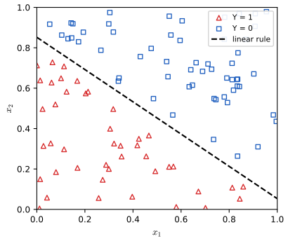
fig_22_1. Download: PDF · SVGExample 22.2 (CORIS). p. 350 The Coronary Risk-Factor Study data of Example 13.17: 462 men, \(Y=1\) for coronary heart disease (160 cases), nine covariates. LDA on systolic blood pressure and cumulative tobacco misclassifies 141 of the 462 men, exactly as in the book (Figure 22.S1 and Example 22.8). The two classes overlap heavily.
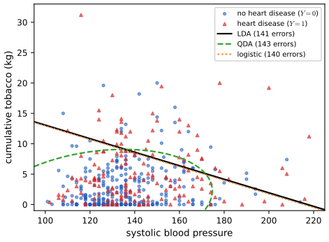
fig_22_s1. Download: PDF · SVG22.2 Error Rates and the Bayes Classifier
Definition 22.3 (error rates) p. 351
The true error rate of \(h\) and its training (empirical) error rate are
\[ L(h)=\P(\{h(X)\ne Y\}), \tag{22.1} \] \[ \hL(h)=\frac1n\sum_{i=1}^n\ind\big(h(X_i)\ne Y_i\big). \tag{22.2} \]p. 351 For \(\cY=\{0,1\}\), the regression function is \(r(x)=\E(Y\given X=x)=\P(Y=1\given X=x)\), and by Bayes' theorem
\[ r(x)=\frac{\pi f_1(x)}{\pi f_1(x)+(1-\pi)f_0(x)},\qquad f_k(x)=f(x\given Y=k),\ \ \pi=\P(Y=1). \tag{22.3} \]Definition 22.4 (the Bayes rule) p. 351
\[ h^*(x)=\begin{cases}1 & r(x)>\tfrac12\\ 0&\text{otherwise,}\end{cases} \tag{22.4} \]equivalently \(h^*(x)=1\) iff \(\P(Y=1\given X=x)>\P(Y=0\given X=x)\) (22.5), iff \(\pi f_1(x)>(1-\pi)f_0(x)\) (22.6). The set \(\{x:r(x)=1/2\}\) is the decision boundary. The name has nothing to do with Bayesian inference.
Theorem 22.5 (the Bayes rule is optimal) p. 352
For every classification rule \(h\), \(L(h^*)\le L(h)\).
Filling the gap 22.1: proof of Theorem 22.5 (Exercise 22.1), and the exact excess risk p. 352
For any measurable \(h:\cX\to\{0,1\}\),
\[ L(h)-L(h^*)=\E\Big[\,|2r(X)-1|\;\ind\{h(X)\ne h^*(X)\}\Big]=\int_{\{h\ne h^*\}}\big|\pi f_1(x)-(1-\pi)f_0(x)\big|\,\d x\ \ \ge 0 , \]with the integral form when \(X\) has a density. The excess error is the "weight" \(|2r-1|\) of the region where \(h\) disagrees with \(h^*\): disagreeing where \(r(x)\approx1/2\) costs almost nothing, disagreeing where the classes are well separated costs a lot.
Proof
Condition on \(X=x\). Given \(X=x\), \(Y\) is Bernoulli\((r(x))\), so for a fixed label \(a\in\{0,1\}\), \(\P(Y\ne a\given X=x)\)
If \(h(x)=h^*(x)\) this is 0. If \(h^*(x)=1\) and \(h(x)=0\), then \(r(x)>1/2\) and the difference is \(-(1-2r(x))=2r(x)-1=|2r(x)-1|\). If \(h^*(x)=0\) and \(h(x)=1\), then \(r(x)\le1/2\) and the difference is \(1-2r(x)=|2r(x)-1|\). So the conditional difference is \(|2r(x)-1|\ind\{h(x)\ne h^*(x)\}\ge0\). Taking expectations over \(X\) (the rule of iterated expectations, Theorem 3.11) gives the identity and \(L(h)\ge L(h^*)\). For the integral form, \(|2r(x)-1|f(x)=|\pi f_1(x)-(1-\pi)f_0(x)|\) by (22.3), with \(f=\pi f_1+(1-\pi)f_0\) the density of \(X\). ∎
The Bayes error itself is \(L(h^*)\)
p. 352 Since the Bayes rule depends on unknown quantities, it must be estimated. The book distinguishes three approaches: (1) empirical risk minimisation: choose \(h\) in a class \(\cH\) to minimise an estimate of \(L(h)\); (2) regression: estimate \(r\) by \(\hr\) and use \(\ind\{\hr(x)>1/2\}\); (3) density estimation: estimate \(f_0,f_1\) and \(\pi\) by \(\hpi=n^{-1}\sum_iY_i\), plug them into (22.3), and threshold at \(1/2\).
Theorem 22.6 (\(K\) classes) p. 352
If \(Y\in\{1,\dots,K\}\), the optimal rule is
\[ h(x)=\argmax_k\P(Y=k\given X=x) \tag{22.7} \] \[ \phantom{h(x)}=\argmax_k\pi_kf_k(x), \tag{22.8} \] \[ \P(Y=k\given X=x)=\frac{f_k(x)\pi_k}{\sum_rf_r(x)\pi_r}, \tag{22.9} \]with \(\pi_r=\P(Y=r)\) and \(f_r(x)=f(x\given Y=r)\).
Filling the gap 22.2: proof of Theorem 22.6 p. 352
Write \(p_k(x)=\P(Y=k\given X=x)\). For any rule, \(\P(h(X)=Y\given X=x)\)
22.3 Gaussian and Linear Classifiers
p. 353 The simplest density-estimation approach takes each class to be Gaussian: \(X\given Y=k\sim\N(\mu_k,\Sigma_k)\), with density
\[ f_k(x)=(2\pi)^{-d/2}|\Sigma_k|^{-1/2}\exp\{-\tfrac12(x-\mu_k)^\T\Sigma_k^{-1}(x-\mu_k)\}. \]Theorem 22.7 (Gaussian classes: QDA) p. 353
If \(X\given Y=0\sim\N(\mu_0,\Sigma_0)\) and \(X\given Y=1\sim\N(\mu_1,\Sigma_1)\), the Bayes rule is
\[ h^*(x)=\begin{cases}1&\text{if } r_1^2<r_0^2+2\log\Big(\dfrac{\pi_1}{\pi_0}\Big)+\log\Big(\dfrac{|\Sigma_0|}{|\Sigma_1|}\Big)\\ 0&\text{otherwise,}\end{cases} \tag{22.10} \] \[ r_k^2=(x-\mu_k)^\T\Sigma_k^{-1}(x-\mu_k),\qquad k=0,1, \tag{22.11} \]the squared Mahalanobis distance of \(x\) from the class mean. Equivalently \(h^*(x)=\argmax_k\delta_k(x)\) with
\[ \delta_k(x)=-\tfrac12\log|\Sigma_k|-\tfrac12(x-\mu_k)^\T\Sigma_k^{-1}(x-\mu_k)+\log\pi_k . \tag{22.12} \]Filling the gap 22.3: proof of Theorem 22.7 (Exercise 22.2), and the plug-in estimates pp. 353–354
(a) The rule (22.10) is (22.6). (b) The book's estimates \(\hpi_k=n_k/n\), \(\hmu_k=\bX_k\) (class means) and \(S_k\)
Proof
(a) Both sides of \(\pi_1f_1(x)>\pi_0f_0(x)\) are positive; take logarithms. Since \(\log(\pi_kf_k(x))\)
(b) The log-likelihood of the joint model factorises into a multinomial part \(\sum_kn_k\log\pi_k\) and, for each class, the Gaussian log-likelihood of that class's \(X_i\). The first is maximised under \(\sum_k\pi_k=1\) by \(\hpi_k=n_k/n\) (Lagrange multiplier). Each Gaussian part is maximised by the sample mean and the covariance with divisor \(n_k\) (the multivariate Normal MLE: the score in \(\mu\) gives \(\bX_k\); with \(\Omega=\Sigma^{-1}\) the profile log-likelihood \(\tfrac{n_k}2\log|\Omega|-\tfrac12\tr(\Omega\,n_kS_k)\) is concave in \(\Omega\) with gradient \(\tfrac{n_k}2(\Omega^{-1}-S_k)\), so \(\widehat\Sigma=S_k\), provided \(S_k\) is invertible, which needs \(n_k>d\)).
(c) \(\delta_1-\delta_0\)
For \(K\) classes (Theorem 22.9 below) the same computation applies to each pair. Companion proofs: Result 4.5 of Applied Statistical Learning and Result 4.10 of Bayesian and Probabilistic Machine Learning.
p. 354 When \(\Sigma_0=\Sigma_1=\Sigma\) (the book's "\(\Sigma_0=\Sigma_0\)" is a slip listed in the author's errata) the Bayes rule is \(h^*(x)=\argmax_k\delta_k(x)\) with
\[ \delta_k(x)=x^\T\Sigma^{-1}\mu_k-\tfrac12\mu_k^\T\Sigma^{-1}\mu_k+\log\pi_k \tag{22.14} \](the book drops the last \(\mu_k\); listed in the errata). The maximum likelihood estimate of \(\Sigma\) is the pooled \(S=(n_0S_0+n_1S_1)/(n_0+n_1)\), and the plug-in rule \(h(x)=\ind\{\delta_1(x)>\delta_0(x)\}\) (22.15) with \(\delta_j(x)\)
Filling the gap 22.4: why a common covariance gives (22.14), and its estimate p. 354
With \(\Sigma_k=\Sigma\) the term \(-\tfrac12\log|\Sigma|\) and the quadratic \(-\tfrac12x^\T\Sigma^{-1}x\) in (22.12) are the same for every \(k\), so they do not affect the arg max. Expanding \(-\tfrac12(x-\mu_k)^\T\Sigma^{-1}(x-\mu_k)\)lda) give the same 2×2 tables, though in general the divisor shifts the threshold relative to \(\log\hpi_k\). ∎
Example 22.8. p. 354 For the CORIS data with systolic blood pressure and tobacco, my LDA and QDA reproduce the book's tables exactly:
| LDA: \(\hh=0\) | LDA: \(\hh=1\) | QDA: \(\hh=0\) | QDA: \(\hh=1\) | |
|---|---|---|---|---|
| \(Y=0\) | 277 | 25 | 272 | 30 |
| \(Y=1\) | 116 | 44 | 113 | 47 |
The training errors are \(141/462=0.305\) and \(143/462=0.310\). With all nine covariates I find 0.253 for LDA and 0.240 for QDA (identical to R's lda and qda), against the book's .27 and .26; the leave-one-out error of LDA is \(125/462=0.271\), which may be what the book reports (Notes on the book). QDA brings little here.
Theorem 22.9 (\(K\) Gaussian classes) p. 355
If \(f_k\) is \(\N(\mu_k,\Sigma_k)\), the Bayes rule is \(\argmax_k\delta_k(x)\) with \(\delta_k\) as in (22.12), now called (22.16); with equal covariances, \(\delta_k(x)\)
pp. 355–356 Fisher's linear discriminant reduces \(X\) to one dimension, \(U=w^\T X\), choosing \(w\) so that the two projected classes are far apart relative to their spread. With \(\mu_j=\E(X\given Y=j)\) and \(\Sigma\) the within-class covariance, \(\E(U\given Y=j)=w^\T\mu_j\) and \(\V(U\given Y=j)=w^\T\Sigma w\), and the separation is the Rayleigh coefficient \(J(w)=\{w^\T(\mu_0-\mu_1)\}^2/w^\T\Sigma w\). It is estimated by
\[ \widehat J(w)=\frac{w^\T\SB w}{w^\T\SW w},\qquad \SB=(\bX_0-\bX_1)(\bX_0-\bX_1)^\T,\quad \SW=\frac{(n_0-1)S_0+(n_1-1)S_1}{(n_0-1)+(n_1-1)}, \tag{22.18} \]with \(S_j\) here the unbiased sample covariances.
Theorem 22.10 (Fisher's direction) p. 356
The vector
\[ w=\SW^{-1}(\bX_0-\bX_1) \tag{22.19} \]maximises \(\widehat J(w)\) (the book says "minimizer"; listed in the errata). \(U=w^\T X=(\bX_0-\bX_1)^\T\SW^{-1}X\) (22.20) is the Fisher linear discriminant function. With the projected midpoint
\[ m=\tfrac12\,w^\T(\bX_0+\bX_1)=\tfrac12(\bX_0-\bX_1)^\T\SW^{-1}(\bX_0+\bX_1), \tag{22.21} \]Fisher's rule is \(h(x)=0\) if \(w^\T x\ge m\) and \(h(x)=1\) if \(w^\T x<m\). It is the LDA rule (22.15) when \(\hpi_0=\hpi_1\). (The book's (22.21) writes \(\SB^{-1}\), which does not exist; see Notes on the book.)
Filling the gap 22.5: proof of Theorem 22.10 p. 356
Proof
Maximiser. Assume \(\SW\) is positive definite and write \(\delta=\bX_0-\bX_1\ne0\). For \(w\ne0\), \(\widehat J(w)=(w^\T\delta)^2/w^\T\SW w\). Put \(v=\SW^{1/2}w\); then \(w^\T\delta=v^\T\SW^{-1/2}\delta\) and, by the Cauchy–Schwarz inequality,
\[ \widehat J(w)=\frac{(v^\T\SW^{-1/2}\delta)^2}{v^\T v}\le\delta^\T\SW^{-1}\delta , \]with equality iff \(v\propto\SW^{-1/2}\delta\), i.e. \(w\propto\SW^{-1}\delta\). So (22.19) attains the maximum \(\delta^\T\SW^{-1}\delta\), and every maximiser is a multiple of it (\(\widehat J\) is scale invariant). Equivalently, \(w\) is the top generalised eigenvector of \(\SB w=\lambda\SW w\), which has only one nonzero eigenvalue because \(\SB\) has rank one.
The rule. \(w^\T\bX_0-w^\T\bX_1\)
Equivalence with LDA. The LDA rule (22.15) says 1 iff \(\delta_1(x)>\delta_0(x)\), i.e.
\[ (\hmu_1-\hmu_0)^\T S^{-1}\Big(x-\tfrac{\hmu_0+\hmu_1}2\Big)>\log\frac{\hpi_0}{\hpi_1}. \]The pooled MLE is \(S=\tfrac{n-2}{n}\SW\), a positive multiple, so with \(\hpi_0=\hpi_1\) the condition is \(w^\T(x-\tfrac{\hmu_0+\hmu_1}2)<0\), i.e. \(w^\T x<m\): Fisher's rule. With unequal proportions LDA shifts the threshold by \(\log(\hpi_0/\hpi_1)\) in these units. ∎
The same argument is Result 4.4 of Bayesian and Probabilistic Machine Learning; the multi-class version (discriminant coordinates) is Result 4.6 of Statistical Learning.
22.4 Linear Regression and Logistic Regression
pp. 356–357 The regression approach estimates \(r(x)=\E(Y\given X=x)\) directly and classifies by
\[ \hh(x)=\begin{cases}1&\hr(x)>\tfrac12\\0&\text{otherwise.}\end{cases} \tag{22.22} \]The crudest choice is the linear model \(Y=\beta_0+\sum_j\beta_jX_j+\epsilon\) (22.23), fitted by least squares, \(\widehat\beta\)
fitted by maximum likelihood with Newton's method (reweighted least squares, Algorithm 13.B).
Filling the gap 22.6: what the least squares classifier estimates p. 357
With two classes coded 0/1, the least squares slope vector is proportional to the LDA direction: \(\widehat\beta_{1:d}=c\,S^{-1}(\hmu_1-\hmu_0)\) for some \(c>0\). So the linear-regression rule draws a hyperplane parallel to LDA's; only the cut-point differs (it equals LDA's when \(n_0=n_1\)).
Proof sketch
Centre the covariates. The slope solves \(T\beta\)
Example 22.11. p. 357 On the CORIS data with all nine covariates (the fit of Example 13.17), logistic regression misclassifies 123 men (0.266, the book's .27) and linear regression 118 (0.255, the book's .26).
Example 22.12. pp. 357–358 A richer model adds all products,
\[ \logit\P(Y=1\given X=x)=\beta_0+\sum_j\beta_jx_j+\sum_{j\le k}\beta_{jk}x_jx_k, \tag{22.25} \]54 terms besides the intercept. Its training error is \(100/462=0.216\) (the book's .22). Whether this is a real improvement is the question of Section 22.8: richer models always fit the training data better.
22.5 Relationship Between Logistic Regression and LDA
pp. 358–359 If both classes are Gaussian with a common covariance, the log-odds are linear in \(x\):
\[ \log\frac{\P(Y=1\given X=x)}{\P(Y=0\given X=x)}=\log\frac{\pi_1}{\pi_0}-\tfrac12(\mu_0+\mu_1)^\T\Sigma^{-1}(\mu_1-\mu_0)+x^\T\Sigma^{-1}(\mu_1-\mu_0)\equiv\alpha_0+\alpha^\T x \](the book prints \(\log(\pi_0/\pi_1)\); see Filling the gap 22.7). Logistic regression assumes exactly this form, \(\beta_0+\beta^\T x\). The two methods differ in how the coefficients are estimated. Since \(f(x,y)=f(x\given y)f(y)=f(y\given x)f(x)\), LDA maximises the full likelihood
\[ \prod_if(x_i,y_i)=\underbrace{\prod_if(x_i\given y_i)}_{\text{Gaussian}}\ \underbrace{\prod_if(y_i)}_{\text{Bernoulli}}, \tag{22.26} \]while logistic regression maximises only the conditional likelihood and ignores the marginal of \(X\):
\[ \prod_if(x_i,y_i)=\underbrace{\prod_if(y_i\given x_i)}_{\text{logistic}}\ \underbrace{\prod_if(x_i)}_{\text{ignored}}. \tag{22.27} \]Logistic regression leaves \(f(x)\) unspecified, so it is more nonparametric than LDA.
Filling the gap 22.7: the log-odds, and what each method gains and loses p. 358
(a) Derivation of the display. (b) Logistic regression is consistent for \((\alpha_0,\alpha)\) under every model with linear log-odds, LDA only under the Gaussian one; under the Gaussian model LDA is more efficient. (c) Linear log-odds hold far beyond the Gaussian case.
Proof
(a) \(\log\{\pi_1f_1(x)/(\pi_0f_0(x))\}\)
(b) The conditional MLE maximises \(\sum_i\log f(y_i\given x_i;\beta)\), whose expectation is maximised at the true \(\beta\) whenever the logistic model is correct, whatever \(f(x)\) is; under the usual regularity conditions it is consistent (Chapter 9 theory applied conditionally on the \(x_i\)). The LDA plug-in \(\widehat\alpha=S^{-1}(\hmu_1-\hmu_0)\) converges to \(\Sigma_{\text{w}}^{-1}(\mu_1-\mu_0)\), the within-class covariance and means of whatever distribution generated the data, which equals the log-odds slope only for Gaussian classes (or special cases). When the Gaussian model holds, LDA uses the information in \(f(x)\) too and its estimate has smaller asymptotic variance; Efron (1975) computed the loss of logistic regression at between one half and two thirds of LDA's efficiency in typical cases. The first demonstration shows both effects: under Gaussian classes LDA is a little better; with a far cluster in one class LDA is biased and logistic regression is not.
(c) If \(f_k(x)=h(x)\exp\{\theta_k^\T T(x)-A(\theta_k)\}\) are members of one exponential family, the log-odds \(\log(\pi_1/\pi_0)\)
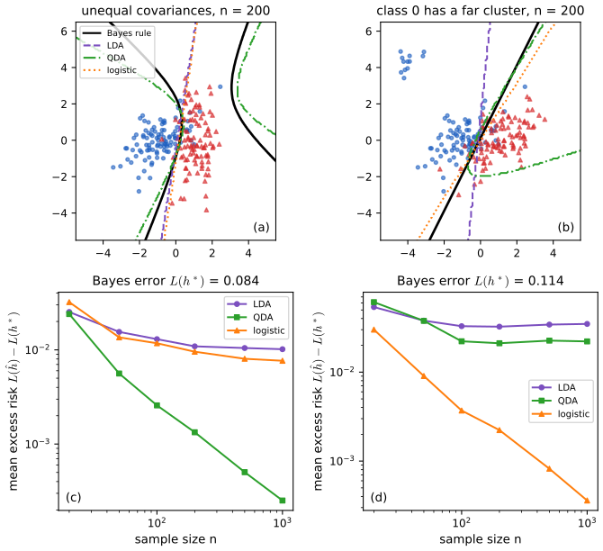
fig_22_s2, learning_curve. Download: PDF · SVGSee also (companion course): the LDA and QDA demo and Result 4.6 of Applied Statistical Learning.
22.6 Density Estimation and Naive Bayes
p. 359 Any density estimates \(\widehat f_k\) can be plugged into \(\argmax_k\hpi_k\widehat f_k(x)\). Nonparametric estimates (kernel estimates, Chapter 20 of the book) are unreliable in high dimensions; the naive Bayes classifier assumes the coordinates of \(X\) independent within each class, \(f_k(x)=\prod_{j=1}^df_{kj}(x_j)\), which turns one \(d\)-dimensional problem into \(d\) one-dimensional ones.
Algorithm 22.B (the naive Bayes classifier) p. 359
- For each class \(k\) and coordinate \(j\), estimate the density \(\widehat f_{kj}\) of \(X_j\) from the cases with \(Y_i=k\).
- Set \(\widehat f_k(x)\)
\({}=\prod_{j=1}^d\widehat f_{kj}(x_j)\) and \(\hpi_k=n^{-1}\sum_i\ind(Y_i=k)\). - Classify by \(\hh(x)=\argmax_k\hpi_k\widehat f_k(x)\).
Filling the gap 22.8: when naive Bayes is right, and why it can classify well when it is wrong p. 359
(a) If the coordinates are conditionally independent given \(Y\), the naive Bayes rule with the true \(f_{kj}\) is the Bayes rule (Theorem 22.6 with \(f_k=\prod_jf_{kj}\)). (b) With Gaussian \(f_{kj}\) it is QDA with diagonal covariance matrices. (c) With discrete \(X_j\) taking values \(1,\dots,L_j\), \(\log\widehat f_k(x)\)
22.7 Trees
pp. 360–361 A classification tree partitions \(\cX\) into rectangles by successive binary splits on one covariate at a time and labels each rectangle (leaf) by majority vote. The book's Figures 22.2 and 22.3 show a hypothetical tree on age and blood pressure and its partition; they are diagrams and are not redrawn. For a split of one covariate at \(t\) into \(A_1=(-\infty,t]\) and \(A_2=(t,\infty)\), let
\[ p_s(j)=\frac{\sum_{i}\ind(Y_i=j,X_i\in A_s)}{\sum_i\ind(X_i\in A_s)},\qquad s=1,2, \tag{22.28} \]and define the impurity of the split and the Gini index of a node by
\[ I(t)=\sum_{s=1}^2\gamma_s, \tag{22.29} \] \[ \gamma_s=1-\sum_{j=0}^1p_s(j)^2 \tag{22.30} \](for \(K\) classes the sum in (22.30) runs over \(j=1,\dots,K\), (22.31)). The split point (and, with several covariates, the covariate) is chosen to minimise the impurity; splitting continues until a stopping rule is met, and each leaf gets the majority label. Standard practice, and the software the book used, weights each child by its size: \(I(t)=\sum_sn_s\gamma_s\); see Filling the gap 22.9.
Filling the gap 22.9: why splitting reduces the weighted impurity, and why the weights matter pp. 360–361
(a) Let \(\phi(p)=1-\sum_jp_j^2\) (Gini) or \(\phi(p)=-\sum_jp_j\log p_j\) (entropy; the deviance of a node is \(2n\phi\)). Both are concave on the probability simplex. For any split of a node with class proportions \(p\) into children of sizes \(n_1,n_2\) and proportions \(p^{(1)},p^{(2)}\), \(p=\tfrac{n_1}np^{(1)}+\tfrac{n_2}np^{(2)}\), so by Jensen's inequality
\[ n_1\phi(p^{(1)})+n_2\phi(p^{(2)})\le n\,\phi(p): \]a split never increases the size-weighted impurity, and decreases it strictly (for strictly concave \(\phi\)) unless both children have the parent's proportions. (b) The book's unweighted \(I(t)=\gamma_1+\gamma_2\) has no such property and favours cutting off a few cases: a child holding three pure cases has \(\gamma=0\), so the sum is about the parent's impurity, while any balanced split leaves two impure children. On the CORIS data the unweighted criterion's best root split on age is \(t=15.5\), which isolates three men, whereas the weighted Gini index chooses \(t=50.5\) and the deviance \(t=31.5\) (Figure 22.S5(b)). (c) The trees below were grown with the deviance and the stopping rules of R's tree package (split a node only if it has at least 10 cases, each child has at least 5, and the deviance falls by more than 1% of the root deviance), which reproduces the book's trees exactly.
Proof of (a)
\(\phi\) is concave: the Gini index is a constant minus the convex function \(\sum_jp_j^2\); the entropy is a sum of the concave functions \(-p\log p\) (second derivative \(-1/p<0\)). The children's proportions average, with weights \(n_s/n\), to the parent's, because counts add. Jensen's inequality for concave functions (Theorem 4.9), \(\sum_sw_s\phi(p^{(s)})\le\phi(\sum_sw_sp^{(s)})\), multiplied by \(n\), is the claim; strict concavity gives strict inequality unless \(p^{(1)}=p^{(2)}\). ∎
Why the Gini index and the deviance are preferred to the misclassification rate for growing (it is piecewise linear, so many splits tie): Result 9.7 of Statistical Learning.
Example 22.13. p. 362 The tree grown on all nine CORIS covariates has 15 leaves and misclassifies 96 men (0.208, the book's .21). Grown on tobacco and age only it has five leaves and 133 errors (0.288, the book's .29); it is the book's Figure 22.4 split for split.
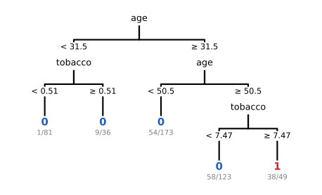
fig_22_4, grow_tree. Download: PDF · SVGLeaves 1 and 2 have the same label: the split on tobacco at 0.51 changes no prediction, but it lowers the deviance (one leaf is nearly pure), which is what the growing criterion rewards. Growing until the leaves are tiny overfits; the size is chosen by an estimate of the true error, as in the next section.
See also (companion course): growing and pruning trees on the spam data in Section 9.2.3 of Statistical Learning and its tree pruning demo.
22.8 Assessing Error Rates and Choosing a Good Classifier
p. 362 The training error \(\hL(\hh)\) of a fitted classifier is biased downward as an estimate of \(L(\hh)\): the classifier was chosen to make it small.
Example 22.14. pp. 362–363 Fit a nested sequence of 18 logistic regressions to the CORIS data: the first \(j\) covariates for \(j=1,\dots,9\) (in the file's order sbp, tobacco, ldl, adiposity, famhist, typea, obesity, alcohol, age), then all nine plus the squares of the first \(s\) covariates, \(s=1,\dots,9\). The training error falls (with small bumps: a better likelihood need not mean fewer misclassifications), the 10-fold cross-validation error falls and then flattens and rises a little.
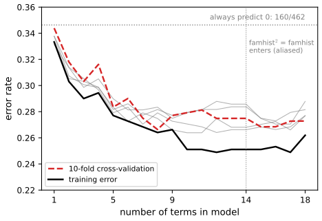
fig_22_5. Download: PDF · SVGpp. 363–364 Cross-validation. Split the data at random into a training set \(\mathcal T\) and a validation set \(\mathcal V\) of size \(m\) (often about 10%); build \(\hh\) from \(\mathcal T\) and estimate its error by
\[ \widehat L(\hh)=\frac1m\sum_{X_i\in\mathcal V}\ind\big(\hh(X_i)\ne Y_i\big). \tag{22.32} \]The book's Figure 22.6 is a diagram of this split and is not redrawn. \(K\)-fold cross-validation divides the data at random into \(K\) chunks (\(K=10\) is common); for each \(k\), the classifier \(\hh^{(k)}\) is built without chunk \(k\) and its error rate \(\widehat L_{(k)}\) on chunk \(k\) is recorded, and
\[ \widehat L(\hh)=\frac1K\sum_{k=1}^K\widehat L_{(k)}. \tag{22.33} \]Filling the gap 22.10: what cross-validation estimates, with an exact interval for the hold-out estimate pp. 363–364
(a) Conditionally on the training set, (22.32) is the proportion of \(m\) independent Bernoulli\((L(\hh))\) trials, so it is unbiased for the true error of the classifier actually built, and by Hoeffding's inequality \(\widehat L(\hh)\pm\sqrt{\log(2/\alpha)/(2m)}\) contains \(L(\hh)\) with probability at least \(1-\alpha\), for every \(m\) and every way of building \(\hh\) from \(\mathcal T\). (b) \(K\)-fold cross-validation is an unbiased estimate of \(\E L(\hh_{n'})\), the expected error of the method trained on \(n'=n(K-1)/K\) cases (when \(K\) divides \(n\)); it estimates the error of the procedure, not of the particular classifier fitted to all \(n\) cases.
Proof
(a) Given \(\mathcal T\), \(\hh\) is a fixed function, and the validation pairs are iid and independent of \(\mathcal T\), so the indicators \(\ind(\hh(X_i)\ne Y_i)\) are iid Bernoulli with mean \(\P(\hh(X)\ne Y\given\mathcal T)=L(\hh)\). Unbiasedness is immediate, and Hoeffding's inequality for a proportion (Theorem 4.5) applies conditionally; integrating over \(\mathcal T\) keeps the bound.
(b) Each \(\widehat L_{(k)}\) is the hold-out estimate for a classifier trained on \(n'\) iid cases, so \(\E\widehat L_{(k)}=\E L(\hh_{n'})\), and the average of the \(K\) has the same mean. The \(\widehat L_{(k)}\) are dependent (their training sets overlap), so no simple variance formula holds; see Section 7.10 of Statistical Learning. ∎
Example 22.15. p. 364 Prune the full CORIS tree by cost complexity: for each penalty \(\alpha\) keep the subtree minimising (training misclassifications) + \(\alpha\times\)(number of leaves). My weakest-link pruning gives subtrees with 15, 10, 9, 6, 5, 4 and 1 leaves at \(\alpha=0,1,3,8,10,12\), exactly R's prune.misclass. Ten-fold cross-validation of this sequence chooses six leaves for three of five random fold assignments and nine for the other two (Figure 22.S5(a)); the book reports six. The six-leaf tree is the book's Figure 22.7.
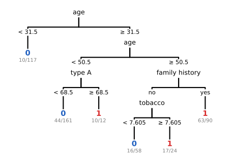
fig_22_7, prune_sequence. Download: PDF · SVG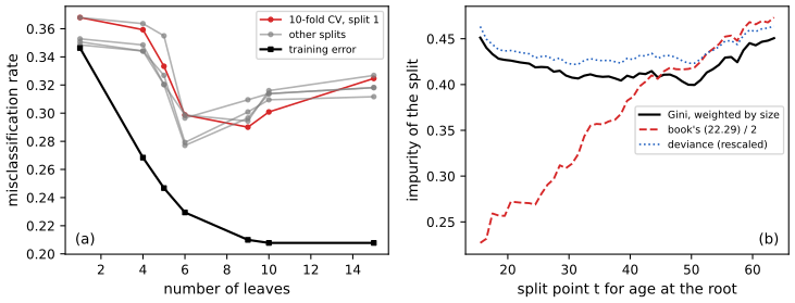
fig_22_s5, tree_cv, gini_root_curves. Download: PDF · SVGSee also (companion course): that cost-complexity pruning gives nested subtrees, Results 9.5 and 9.6 of Statistical Learning.
pp. 365–366 Probability inequalities. For a class \(\cH\) of classifiers, empirical risk minimisation chooses
\[ \hh=\argmin_{h\in\cH}\hL(h)=\argmin_{h\in\cH}\Big(\frac1n\sum_i\ind(h(X_i)\ne Y_i)\Big). \tag{22.34} \]For a single fixed \(h\), \(n\hL(h)\) is Binomial\((n,L(h))\), and Hoeffding's inequality gives, for every \(\epsilon>0\),
\[ \P\big(|\widehat p-p|>\epsilon\big)\le2e^{-2n\epsilon^2}, \tag{22.35} \]\(\widehat p\) the mean of \(n\) Bernoulli\((p)\) variables. But \(\hh\) is chosen using the data, so (22.35) does not apply to it directly.
Theorem 22.16 (uniform convergence, finite class) p. 366
If \(\cH\) is finite with \(m\) elements, \(\P\big(\max_{h\in\cH}|\hL(h)-L(h)|>\epsilon\big)\)
Theorem 22.17 (a confidence interval for the chosen classifier) p. 366
With \(\epsilon=\sqrt{\tfrac1{2n}\log\tfrac{2m}\alpha}\), \(\hL(\hh)\pm\epsilon\) is a \(1-\alpha\) confidence interval for \(L(\hh)\).
Filling the gap 22.11: why the union bound is needed, and what it buys p. 366
The book's proof is complete: the event \(\{\max_h|\hL(h)-L(h)|>\epsilon\}\) is the union of the \(m\) events \(\{|\hL(h)-L(h)|>\epsilon\}\), whose probabilities add to at most \(m\cdot2e^{-2n\epsilon^2}\) by (22.35) (Boole's inequality), and since \(\hh\in\cH\), \(|\hL(\hh)-L(\hh)|\le\max_h|\hL(h)-L(h)|\). Setting \(2me^{-2n\epsilon^2}=\alpha\) gives the \(\epsilon\) of Theorem 22.17. Three remarks:
- Why the uniform statement. \(n\hL(\hh)\) is not Binomial\((n,L(\hh))\): given the selection, the data that made \(\hh\) look good are over-represented. The uniform bound covers the chosen classifier because it covers all of them; the interval holds for every selection rule, not only for empirical risk minimisation.
- The price. \(\epsilon\) grows only like \(\sqrt{\log m}\): squaring the size of the class roughly doubles \(\epsilon^2\). The bound is conservative because nearly identical classifiers are counted as if their deviations were unrelated; the second demonstration shows the actual largest deviation well inside it.
- Excess risk of ERM. On the same event, \(L(\hh)\)
\({}\le\hL(\hh)+\epsilon\) \({}\le\hL(h)+\epsilon\) \({}\le L(h)+2\epsilon\) for every \(h\in\cH\): with probability \(1-\alpha\), ERM is within \(2\epsilon\) of the best classifier in \(\cH\). This is the reason to choose by training error at all. ∎
Related: the sample size needed for a finite class, Result 7.11 of Bayesian and Probabilistic Machine Learning.
pp. 366–367 For infinite classes (all linear rules, say) the union bound is useless, and the size of \(\cH\) is replaced by a combinatorial count. For a class \(\cA\) of sets and a finite set \(F=\{x_1,\dots,x_n\}\), let
\[ N_\cA(F)=\#\{F\cap A:\ A\in\cA\} \tag{22.36} \]be the number of subsets of \(F\) "picked out" by \(\cA\), and define the shatter coefficient
\[ s(\cA,n)=\max_{F\in\mathcal F_n}N_\cA(F), \tag{22.37} \]\(\mathcal F_n\) the sets of \(n\) points. With \(P_n(A)=n^{-1}\sum_i\ind(X_i\in A)\) the empirical measure:
Theorem 22.18 (Vapnik and Chervonenkis 1971) p. 367
For any \(P\), \(n\) and \(\epsilon>0\),
\[ \P\Big(\sup_{A\in\cA}|P_n(A)-P(A)|>\epsilon\Big)\le8\,s(\cA,n)\,e^{-n\epsilon^2/32}. \tag{22.38} \]Theorem 22.19 (the VC bound for classifiers) p. 367
With \(s(\cH,n)=s(\cA,n)\) for \(\cA=\{\{x:h(x)=1\}:h\in\cH\}\), \(\P(\sup_{h\in\cH}|\hL(h)-L(h)|>\epsilon)\)
Filling the gap 22.12: proof sketch of the VC theorem, and from sets to classifiers p. 367
The book omits the proof ("very elegant, but long"). Here is its structure with each step stated precisely; the constants follow Devroye, Györfi and Lugosi (1996, Theorem 12.5), where all details are written out.
Proof sketch
Step 1 (symmetrisation by a ghost sample). Let \(X'_1,\dots,X'_n\) be an independent copy of the sample, with empirical measure \(P'_n\). For \(n\epsilon^2\ge2\),
\[ \P\Big(\sup_A|P_n(A)-P(A)|>\epsilon\Big)\le2\,\P\Big(\sup_A|P_n(A)-P'_n(A)|>\tfrac\epsilon2\Big). \]Reason: on the event that some \(A^*\) (chosen from the first sample) has \(|P_n(A^*)-P(A^*)|>\epsilon\), Chebyshev's inequality applied to \(P'_n(A^*)\), which is independent of the first sample, gives \(|P'_n(A^*)-P(A^*)|\le\epsilon/2\) with conditional probability at least \(1-1/(n\epsilon^2)\ge1/2\), and then \(|P_n(A^*)-P'_n(A^*)|>\epsilon/2\). The point: the right side involves only the \(2n\) sample points, not \(P\).
Step 2 (random signs). Swapping \(X_i\) and \(X'_i\) does not change the joint distribution, so with independent random signs \(\sigma_i=\pm1\),
\[ \P\Big(\sup_A|P_n(A)-P'_n(A)|>\tfrac\epsilon2\Big)=\P\Big(\sup_A\Big|\frac1n\sum_i\sigma_i\big(\ind_A(X_i)-\ind_A(X'_i)\big)\Big|>\tfrac\epsilon2\Big)\le2\,\P\Big(\sup_A\Big|\frac1n\sum_i\sigma_i\ind_A(X_i)\Big|>\tfrac\epsilon4\Big). \]Step 3 (condition and count). Condition on \(X_1,\dots,X_n\). The supremum now ranges over at most \(N_\cA(\{X_1,\dots,X_n\})\le s(\cA,n)\) distinct vectors \((\ind_A(X_i))_i\): this is where an infinite class becomes finite. Apply the union bound over them.
Step 4 (Hoeffding). For each fixed vector, \(\frac1n\sum_i\sigma_i\ind_A(X_i)\) is an average of independent mean-zero terms in \([-1,1]\), so Hoeffding's inequality (Theorem 4.4) gives \(\P(|\cdot|>\epsilon/4)\)
From sets to classifiers. Apply (22.38) to the pairs \(Z=(X,Y)\) and the sets \(B_h=\{(x,y):h(x)\ne y\}\): \(P(B_h)=L(h)\) and \(P_n(B_h)=\hL(h)\). On \(n\) points \((x_i,y_i)\), \(B_h\) picks out \(\{i:h(x_i)\ne y_i\}\), which is determined by, and determines, \(\{i:h(x_i)=1\}\); so the shatter coefficient of \(\{B_h\}\) is at most \(s(\cH,n)\). This is Theorem 22.19, and solving \(8s(\cH,n)e^{-n\epsilon^2/32}=\alpha\) gives \(\epsilon_n\). ∎
The constants are poor: for unions of two intervals and \(n=200\) the VC half-width is 1.9, and even at \(n=5000\) it is about twenty times the actual largest deviation (second demonstration). Better constants exist (Devroye et al. 1996, Chapter 12), but the qualitative message, \(\epsilon_n\approx\sqrt{v\log n/n}\), is the useful one. The companion derivation: Filling the gap 7.7 of Statistical Learning.
Definition 22.20 (VC dimension) p. 367
If \(s(\cA,n)=2^n\) for all \(n\), \(\VC(\cA)=\infty\); otherwise \(\VC(\cA)\) is the largest \(k\) with \(s(\cA,k)=2^k\) (the book writes \(s(\cA,n)=2^k\), a slip). Equivalently it is the size of the largest set shattered by \(\cA\) (every subset picked out). For classifiers, \(\VC(\cH)=\VC(\{\{h=1\}:h\in\cH\})\).
Theorem 22.21 (Sauer's lemma) p. 368
If \(\cA\) has finite VC dimension \(v\), then \(s(\cA,n)\le\sum_{i=0}^v\binom ni\le n^v+1\).
Filling the gap 22.13: proof of Sauer's lemma (Theorem 22.21) p. 368
Proof
Part 1: \(N_\cA(F)\le\sum_{i\le v}\binom ni\). Fix \(F\) with \(|F|=n\) and let \(\mathcal T=\{F\cap A:A\in\cA\}\), a family of subsets of \(F\). Claim (Pajor's lemma): \(\mathcal T\) shatters at least \(|\mathcal T|\) subsets of \(F\) (the empty set counts as shattered when \(\mathcal T\ne\emptyset\)). Since every shattered set has at most \(v\) elements, and there are \(\sum_{i\le v}\binom ni\) such subsets, the bound follows.
Proof of the claim by induction on \(n\). For \(n=0\) it is clear. For \(n\ge1\) pick \(x\in F\), \(F'=F\setminus\{x\}\), and define two families of subsets of \(F'\): \(\mathcal T_0=\{T\setminus\{x\}:T\in\mathcal T\}\) and \(\mathcal T_1\)
Part 2: \(\Phi_v(n)=\sum_{i\le v}\binom ni\le n^v+1\) for \(n,v\ge1\). If \(v\ge n\), \(\Phi_v(n)=2^n\le n^n+1\le n^v+1\). Otherwise induct on \(n\): \(\Phi_v(1)=2\). For \(v=1\), \(\Phi_1(n)=n+1\). For \(v\ge2\) and \(n>v\), Pascal's rule \(\binom ni=\binom{n-1}i+\binom{n-1}{i-1}\) gives \(\Phi_v(n)\)
So a class of finite VC dimension has polynomially many patterns on \(n\) points, and \(\epsilon_n^2\)
Examples 22.22–22.25. p. 368 Half-lines \((-\infty,a]\): VC dimension 1 (two points \(x<y\) cannot give \(\{y\}\)); \(s=n+1\). Closed intervals: 2 (for \(x<y<z\), \(\{x,z\}\) cannot be picked out); \(s=1+n(n+1)/2\). Half-planes: 3. Axis-parallel rectangles: 4. Unions of at most \(k\) intervals: \(2k\), with \(s=\sum_{j\le k}\binom{n+1}{2j}\) exactly (the count of 0/1 strings of length \(n\) with at most \(k\) runs of ones), which the second demonstration uses.
Theorem 22.26 (linear classifiers) p. 368
Linear classifiers \(h(x)=\ind\{a_0+a^\T x>0\}\) on \(\R^d\) have VC dimension \(d+1\). Hence, by Theorems 22.19 and 22.21, \(\hL(\hh)\pm\epsilon_n\) with \(\epsilon_n^2\)
Filling the gap 22.14: the VC dimensions of Examples 22.24–22.25 and of half-spaces p. 368
Proof
Half-spaces in \(\R^d\) shatter \(d+1\) points. Take \(0,e_1,\dots,e_d\). For a target subset \(S\), put \(a_j=+1\) if \(e_j\in S\) and \(-1\) otherwise, and \(a_0=+\tfrac12\) if \(0\in S\), \(-\tfrac12\) otherwise. Then \(a_0+a^\T e_j=a_0\pm1\) has the sign of \(a_j\), and \(a_0+a^\T0=a_0\) the right sign.
No \(d+2\) points are shattered. By Radon's theorem, any \(d+2\) points \(x_1,\dots,x_{d+2}\) in \(\R^d\) split into two groups \(I,J\) whose convex hulls meet. (Proof: the \(d+2\) vectors \((x_i,1)\in\R^{d+1}\) are linearly dependent, \(\sum_i\lambda_i(x_i,1)=0\) with \(\lambda\ne0\); put \(I=\{\lambda_i>0\}\), \(J=\{\lambda_i\le0\}\), \(c=\sum_{I}\lambda_i=-\sum_J\lambda_i>0\); then \(\sum_I(\lambda_i/c)x_i=\sum_J(-\lambda_i/c)x_i\) is in both hulls.) If a half-space contained exactly the points of \(I\), it would contain their convex hull and its complement (also convex) would contain the hull of \(J\): impossible, since the hulls meet. So the labeling "\(I\) in, \(J\) out" cannot be realised.
Example 22.24 (half-planes, \(d=2\)) is the case \(d=2\): three non-collinear points are shattered, four are not (for a convex quadrilateral the two diagonals cannot be separated; otherwise one point is inside the triangle of the others and cannot be excluded alone). By Cover's (1965) count, \(n\) points in general position in the plane have exactly \(2\sum_{i\le2}\binom{n-1}i\) dichotomies by half-planes, 14 for \(n=4\); I confirmed this by linear programming for \(n=3,\dots,7\).
Example 22.25 (rectangles). The book says "any 4 point set can be shattered"; only some can (four collinear points cannot: no rectangle picks out the first and third without the second), and that is all the definition requires. The four points of a diamond \((0,\pm1),(\pm1,0)\) are shattered. For five points, choose one leftmost, one rightmost, one highest and one lowest (at most four points); any rectangle containing these contains their bounding box and hence the fifth point, so "all but the fifth" cannot be picked out. (The book's "one point that is not leftmost, rightmost, uppermost or lowermost" needs this choice of extreme points when there are ties.) So \(\VC=4\).
The companion proof of the half-space result: Result 7.12 of Statistical Learning. ∎
For the CORIS data with \(d=2\), \(n=462\) and \(\alpha=0.05\), Theorem 22.26 gives \(\epsilon_n=1.28\): a vacuous interval for an error rate. The Hoeffding hold-out interval of Filling the gap 22.10 with a validation set of the same size would have half-width 0.063. VC bounds are tools for understanding rates, not for reporting error rates on samples of this size.
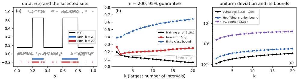
fig_22_s3, intervals_experiment. Download: PDF · SVG22.9 Support Vector Machines
pp. 368–369 Code the labels as \(Y\in\{-1,+1\}\) and write a linear classifier as \(h(x)=\sgn(H(x))\), \(H(x)=a_0+\sum_{i=1}^da_ix_i\). The data are linearly separable if some hyperplane separates the two classes strictly.
Lemma 22.27 p. 369
The data can be separated by a hyperplane iff there is \(H(x)=a_0+\sum_ia_ix_i\) with
\[ Y_iH(X_i)\ge1,\qquad i=1,\dots,n. \tag{22.39} \]p. 369 Among the many separating hyperplanes, the maximum margin hyperplane is the one farthest from the closest point; the margin is that distance, and the points at that distance are the support vectors (Figure 22.8).
Theorem 22.28 p. 369
The hyperplane that separates the data and maximises the margin is found by minimising \(\tfrac12\sum_{j=1}^da_j^2\) subject to (22.39).
Filling the gap 22.15: Lemma 22.27 and Theorem 22.28 p. 369
Proof
Lemma 22.27. If \(W(x)=b_0+b^\T x\) separates strictly, \(Y_iW(X_i)>0\) for all \(i\); with finitely many points \(c=\min_iY_iW(X_i)>0\), and \(H=W/c\) satisfies (22.39). Conversely (22.39) gives \(Y_iH(X_i)\ge1>0\): strict separation.
Distance to a hyperplane. The Euclidean distance from \(x\) to \(\{z:a_0+a^\T z=0\}\) is \(|a_0+a^\T x|/\|a\|\): the closest point is \(x-\tfrac{H(x)}{\|a\|^2}a\) (move along the normal \(a\) until \(H=0\)), at distance \(|H(x)|/\|a\|\).
Theorem 22.28. The margin of a separating \((a_0,a)\) is \(\rho(a_0,a)=\min_iY_i(a_0+a^\T X_i)/\|a\|\), which is unchanged by rescaling \((a_0,a)\). Every separating hyperplane can be rescaled so that \(\min_iY_iH(X_i)=1\), and then \(\rho=1/\|a\|\). So maximising the margin over separating hyperplanes is maximising \(1/\|a\|\) over \((a_0,a)\) with \(\min_iY_iH(X_i)=1\); and relaxing the equality to (22.39) changes nothing, because if \(\min_iY_iH(X_i)=c>1\) then \((a_0,a)/c\) is also feasible with smaller norm. Maximising \(1/\|a\|\) is minimising \(\tfrac12\|a\|^2\). The problem is a strictly convex quadratic in \(a\) with linear constraints, so the optimal \(a\) is unique; \(a_0\) is then unique too (Filling the gap 22.16). ∎
Companion proofs: Result 9.2 of Applied Statistical Learning and Result 7.1 of Bayesian and Probabilistic Machine Learning.
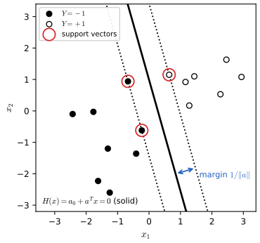
fig_22_8. Download: PDF · SVGTheorem 22.29 (the dual problem) pp. 369–370
Let \(\widehat H(x)\)
subject to \(\alpha_i\ge0\) and \(\sum_i\alpha_iY_i=0\). The \(X_i\) with \(\widehat\alpha_i\ne0\) are the support vectors. \(\widehat a_0\) solves \(\widehat\alpha_i\{Y_i(X_i^\T\widehat a+\widehat a_0)-1\}\)
Filling the gap 22.16: deriving the dual, the optimality conditions, and the weak-duality sandwich pp. 369–370
Derivation
Lagrangian. For \(\alpha\ge0\) let \(\mathcal L(a_0,a,\alpha)\)
which is (22.40), to be maximised over \(\alpha\ge0\) with \(\sum_i\alpha_iY_i=0\).
Strong duality and KKT. The constraints are affine and (if the data are separable) feasible, so Slater's condition in its linear form holds and \(\max g=P^*\), with the maximum attained; equivalently the Karush–Kuhn–Tucker conditions characterise the solutions: primal feasibility (22.39), \(\alpha_i\ge0\), stationarity \(a=\sum_i\alpha_iY_iX_i\) and \(\sum_i\alpha_iY_i=0\), and complementary slackness \(\alpha_i\{Y_i(a_0+a^\T X_i)-1\}=0\). The last says that only points on the margin (\(Y_iH(X_i)=1\)) can have \(\alpha_i>0\): these are the support vectors, and removing any other point does not change the solution. Since some \(\alpha_i>0\) (otherwise \(a=0\), not feasible), \(a_0=Y_i-a^\T X_i\) for any support vector, which is the corrected equation of the theorem.
Two identities. At the optimum, complementary slackness summed over \(i\) gives \(\sum_i\alpha_iY_iH(X_i)=\sum_i\alpha_i\); the left side is \(a_0\sum_i\alpha_iY_i+a^\T\sum_i\alpha_iY_iX_i\)
The sandwich used by the third demonstration. For any dual-feasible \(\alpha\), \(g(\alpha)\le P^*\). Moreover, let \(w=\sum_i\alpha_iY_iX_i\) and \(s_i=w^\T X_i\). If \(\gamma\)
Companion derivations: Results 7.2 and 7.3 of Bayesian and Probabilistic Machine Learning, Result 9.3 of Applied Statistical Learning, and Result 12.1 of Statistical Learning.
Algorithm 22.A (sequential minimal optimisation with the maximal violating pair)
Write the dual as minimising \(f(\alpha)\)
- \(I_{\uparrow}\)
\({}=\{t:Y_t\) \({}=1,\alpha_t\) \({}<C\}\cup\{t:Y_t\) \({}=-1,\alpha_t\) \({}>0\}\), \(I_{\downarrow}\) \({}=\{t:Y_t\) \({}=-1,\alpha_t\) \({}<C\}\cup\{t:Y_t\) \({}=1,\alpha_t\) \({}>0\}\); \(i=\argmax_{t\in I_\uparrow}(-Y_tG_t)\), \(j=\argmin_{t\in I_\downarrow}(-Y_tG_t)\). - Stop if the violation \(\Delta=-Y_iG_i+Y_jG_j\) is below a tolerance: this is the KKT condition.
- Move along \(\alpha_i\mathrel{+}=Y_it\), \(\alpha_j\mathrel{-}=Y_jt\), which keeps \(\sum\alpha_kY_k=0\); the exact minimiser is \(t=\Delta/\eta\) with \(\eta=K_{ii}+K_{jj}-2K_{ij}\), clipped so that both stay in \([0,C]\).
- Update \(G\mathrel{+}=t(Y_iQ_{\cdot i}-Y_jQ_{\cdot j})\) and repeat.
Each step decreases \(f\) (the direction has slope \(-\Delta<0\)), so the dual value \(g=-f\) rises; with the maximal violating pair the iteration converges to the optimum (Keerthi et al. 2001). This is the algorithm of LIBSVM, implemented in smo; on the spam data it matches scikit-learn's dual value.
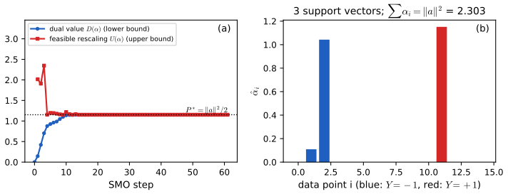
fig_22_s4, smo, duality_bounds. Download: PDF · SVGpp. 370–371 If no hyperplane separates the data, the constraints are relaxed to
\[ Y_iH(X_i)\ge1-\xi_i,\qquad\xi_i\ge0,\qquad i=1,\dots,n, \tag{22.41} \]with slack variables \(\xi_i\), and the objective becomes \(\tfrac12\|a\|^2+c\sum_i\xi_i\). The dual is again (22.40), now subject to \(0\le\alpha_i\le c\) and \(\sum_i\alpha_iY_i=0\) (the book writes \(0\le\xi_i\le c\); the bound is on the multipliers). The constant \(c\) controls how much overlap is tolerated.
Filling the gap 22.17: where the box \(0\le\alpha_i\le c\) comes from p. 371
With multipliers \(\alpha_i\ge0\) for (22.41) and \(\mu_i\ge0\) for \(\xi_i\ge0\), the Lagrangian is \(\tfrac12\|a\|^2+c\sum\xi_i\)
22.10 Kernelization
pp. 371–372 Map the covariates into a higher-dimensional space \(\cZ\) by \(z=\phi(x)\) and use a linear classifier there: it is a nonlinear classifier in \(\cX\). In the book's example \(\phi(x)=(x_1^2,\sqrt2x_1x_2,x_2^2)\) maps \(\R^2\) to \(\R^3\), and classes separated by an ellipse in \(\cX\) become separated by a plane in \(\cZ\) (Figure 22.9). The computational cost of a large \(\cZ\) disappears because (i) many classifiers, such as the SVM dual and Fisher's discriminant, use the data only through inner products, and (ii) inner products in \(\cZ\) can often be computed in \(\cX\):
\[ \langle\phi(x),\phi(\tilde x)\rangle=x_1^2\tilde x_1^2+2x_1\tilde x_1x_2\tilde x_2+x_2^2\tilde x_2^2=\langle x,\tilde x\rangle^2\equiv K(x,\tilde x). \]So: find a kernel \(K\) with \(K(x,\tilde x)\)
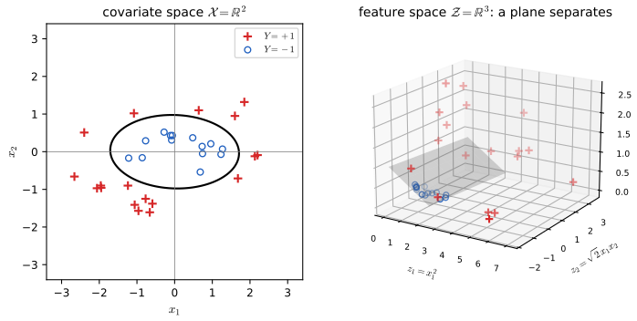
fig_22_9. Download: PDF · SVGFilling the gap 22.18: counting features, Mercer's condition, and which kernels qualify pp. 371–373
(a) The number of monomials of degree exactly 4 in \(d=256\) variables is \(\binom{256+3}{4}=183{,}181{,}376\), the book's number (stars and bars). Evaluating \(\langle x,\tilde x\rangle^4\) costs 257 multiplications.
(b) A symmetric \(K\) is a kernel (an inner product of some feature map into a Hilbert space) iff it is positive semi-definite: every matrix \([K(x_i,x_j)]_{i,j\le m}\) is positive semi-definite. "If": the feature map \(x\mapsto K(\cdot,x)\) into the completion of the span of these functions, with \(\langle K(\cdot,x),K(\cdot,\tilde x)\rangle\)
(c) Positive semi-definite kernels are closed under sums, positive multiples, products (Schur's product theorem: the entrywise product of PSD matrices is PSD) and limits. Hence \((\langle x,\tilde x\rangle+a)^r\) with \(a\ge0\) is a kernel, and so is \(\exp(\langle x,\tilde x\rangle/\sigma^2)\)
The companion treatment: Result 12.4 of Statistical Learning and Result 9.6 of Applied Statistical Learning.
pp. 373–375 Kernel Fisher discriminant. Replace \(X_i\) by \(Z_i=\phi(X_i)\) in (22.18) and maximise
\[ \widehat J(w)=\frac{w^\T\widetilde S_Bw}{w^\T\widetilde S_Ww} \tag{22.42} \]with \(\widetilde S_B,\widetilde S_W\) the between and within matrices of the \(Z_i\). Writing \(w=\sum_i\alpha_iZ_i\), with \(M_j(i)=n_j^{-1}\sum_sK(X_i,X_s)\ind(Y_s=j)\), \(M=(M_0-M_1)(M_0-M_1)^\T\) and \(N=\sum_jK_j(I-\tfrac1{n_j}\mathbf 1)K_j^\T\) (\(K_j\) the \(n\times n_j\) matrix of kernel values with the cases of class \(j\)), the problem becomes maximising \(\alpha^\T M\alpha/\alpha^\T N\alpha\), solved by \(\alpha=(N+bI)^{-1}(M_0-M_1)\) with a small ridge \(b\); the projection of a new \(x\) is \(\sum_i\alpha_iK(X_i,x)\) (Mika et al. 1999). The kernelized SVM maximises
\[ \sum_{i=1}^n\alpha_i-\frac12\sum_{i=1}^n\sum_{k=1}^n\alpha_i\alpha_kY_iY_kK(X_i,X_k) \tag{22.43} \]under the same constraints, and \(\widehat H(x)\)
Filling the gap 22.19: why the optimal \(w\) lies in the span of the \(Z_i\), and where \(M\) and \(N\) come from p. 374
Decompose \(w=w_\parallel+w_\perp\) with \(w_\parallel\) in the span of \(Z_1,\dots,Z_n\) and \(w_\perp\) orthogonal to it. Every quantity in (22.42) is a sum of terms \(w^\T(Z_i-\bar Z_j)\) or \(w^\T(\bar Z_0-\bar Z_1)\), and \(w_\perp\) is orthogonal to all of these vectors, so \(\widehat J(w)=\widehat J(w_\parallel)\): nothing is lost by taking \(w=\sum_i\alpha_iZ_i\). Then \(w^\T\bar Z_j\)
22.11 Other Classifiers
p. 375 \(k\)-nearest neighbours classifies \(x\) by majority vote among the \(k\) training points closest to \(x\), \(k\) chosen by cross-validation (Exercise 22.9). As \(n\to\infty\) with \(k\to\infty\) and \(k/n\to0\) it is universally consistent (Stone 1977); with \(k=1\) its asymptotic error is at most twice the Bayes error (Cover and Hart 1967; Result 13.7 of Statistical Learning). In high dimensions neighbours are far away (Exercise 22.10).
p. 375 Bagging (bootstrap aggregation; Breiman 1996): fit \(\hh_b\) to each of \(B\) bootstrap samples and vote, \(\hh(x)=\ind\{B^{-1}\sum_b\hh_b(x)\ge1/2\}\). It reduces variance, and helps most for unstable classifiers such as trees (Exercise 22.11; when voting helps under 0–1 loss: Result 8.13 of Statistical Learning).
Algorithm 22.C (AdaBoost; Freund and Schapire 1997) pp. 375–376
Labels \(Y_i\in\{-1,1\}\), a class \(\cH\) of classifiers with values \(\pm1\) (e.g. one-split trees, "stumps").
- Set \(w_i=1/n\).
- For \(j=1,\dots,J\): (a) fit \(h_j\) to the data with weights \(w_i\); (b) \(\widehat L_j\)
\({}=\sum_iw_i\ind(Y_i\ne h_j(X_i))/\sum_iw_i\); (c) \(\alpha_j=\log\{(1-\widehat L_j)/\widehat L_j\}\); (d) \(w_i\leftarrow w_ie^{\alpha_j\ind(Y_i\ne h_j(X_i))}\). - Output \(\hh(x)=\sgn\big(\sum_{j=1}^J\alpha_jh_j(x)\big)\).
Filling the gap 22.20: why boosting reduces the training error (bias) p. 376
If every weighted error satisfies \(\widehat L_j\le\tfrac12-\gamma_j\), the training error of the boosted classifier after \(J\) rounds is at most
\[ \prod_{j=1}^J2\sqrt{\widehat L_j(1-\widehat L_j)}=\prod_{j=1}^J\sqrt{1-4\gamma_j^2}\le\exp\Big(-2\sum_{j=1}^J\gamma_j^2\Big). \]So any fixed edge over random guessing drives the training error to zero exponentially fast: this is the precise sense in which boosting reduces bias.
Proof
Let \(F(x)=\tfrac12\sum_j\alpha_jh_j(x)\) (the factor \(\tfrac12\) does not change the sign). With \(\beta_j=\alpha_j/2\), the update \(w_i\leftarrow w_ie^{\alpha_j\ind(Y_i\ne h_j)}\) equals \(w_ie^{-\beta_jY_ih_j(X_i)}\) times \(e^{\beta_j}\), a factor common to all \(i\) that cancels on normalising. So the normalised weights after round \(J\) are \(w_i^{(J+1)}=e^{-Y_iF(X_i)}/(n\prod_jZ_j)\), with \(Z_j\)
Confirmed numerically on the spam data at every round. That boosting is forward stagewise fitting of the exponential loss, and the same bound: Result 10.3 of Statistical Learning.
p. 376 Neural networks in their simplest form are the nonlinear regression models \(Y\)
22.12 Bibliographic Remarks
p. 377 The book recommends Hastie, Tibshirani and Friedman (2001) for methods, Devroye, Györfi and Lugosi (1996) and Vapnik (1998) for theory, and Schölkopf and Smola (2002) and Herbrich (2002) for kernels. The VC theorem is Vapnik and Chervonenkis (1971); Sauer's lemma is due independently to Sauer (1972), Shelah (1972) and Vapnik and Chervonenkis; the proof above follows Pajor's shattering argument.
Notes on the book
Several slips of Chapter 22 are in the author's errata lists; the others are mine, each with the evidence.
Pages 355–356, Theorem 22.10 and (22.21)
"Minimizer" should be "maximizer", and \(X\) should be lower case in Fisher's rule (both listed in the author's errata). The midpoint (22.21) is printed as \(m\)
Page 358, Section 22.5: the prior ratio in the log-odds
The intercept of the LDA log-odds is \(\log(\pi_1/\pi_0)-\tfrac12(\mu_0+\mu_1)^\T\Sigma^{-1}(\mu_1-\mu_0)\), not \(\log(\pi_0/\pi_1)-\dots\) (Filling the gap 22.7(a); confirmed numerically with \(\pi_1=0.3\)). Not in the errata lists.
Pages 353–355: Gaussian classifiers
"Manalahobis" should be "Mahalanobis"; \(\Sigma_0=\Sigma_0\) should be \(\Sigma_0=\Sigma_1\); (22.14) and (22.17) are missing the final \(\mu_k\) (all listed in the errata). Also: in (22.11) the index should run over \(i=0,1\), not \(1,2\); and the text says "sample estimates of \(\pi,\mu_1,\mu_2,\Sigma_0,\Sigma_1\)" where \(\mu_0,\mu_1\) are meant. Not in the errata lists.
Page 354, Example 22.8: the all-covariate error rates
The two-covariate tables are reproduced exactly. With all nine covariates the training errors are 0.253 (LDA) and 0.240 (QDA), the same with R's lda and qda, against the book's .27 and .26. The leave-one-out error of LDA is 0.271, which matches .27; the leave-one-out error of QDA is 0.290 and equal-prior QDA gives 0.264, so I cannot tell how .26 was obtained. Not an error of method, but the numbers are not training errors.
Pages 360–361, (22.29): the impurity of a split
As printed, \(I(t)=\gamma_1+\gamma_2\) sums the two children's Gini indices without weights. The standard criterion (and the software that produced Figures 22.4 and 22.7) weights them by size, \(n_1\gamma_1+n_2\gamma_2\). The unweighted version prefers to split off a handful of cases: on the CORIS data its best root split on age isolates three men (Filling the gap 22.9, Figure 22.S5(b)). Not in the errata lists.
Page 363, Figure 22.5: the jump of the cross-validation curve
The book's dashed curve jumps to about 0.345 at model 14 and stays there. Model 14 is the first to add the square of famhist, a 0/1 variable equal to its own square, so its design matrix is singular. The error 0.346 is exactly that of the classifier that always predicts 0 (\(160/462\)). Dropping the aliased column, as R's glm does, the cross-validation error stays between 0.27 and 0.28 (Figure 22.5). The book's fits apparently failed on the singular designs. Also, the book's first training error (about .345) differs from mine (0.333 for systolic blood pressure alone). My explanation, not in the errata lists.
Pages 366–368: the inequalities and VC dimension
In the proof of Theorem 22.16 the sum should run over \(h\in\cH\), not "\(H\in\cH\)". In Definition 22.20, "the largest \(k\) for which \(s(\cA,n)=2^k\)" should read \(s(\cA,k)=2^k\). In Example 22.25 "any 4 point set can be shattered" should be "some 4 point set" (four collinear points cannot be), and the five-point argument needs extreme points chosen when there are ties (Filling the gap 22.14). In Theorem 22.26 the interval is \(\hL(\hh)\pm\epsilon_n\), centred at the training error, not at \(L(\hh)\). Not in the errata lists.
Pages 370–375: the support vector machine and kernels
In Theorem 22.29, \(\widehat a_0\) solves \(\widehat\alpha_i\{Y_i(X_i^\T\widehat a+\widehat a_0)-1\}\)
Other points
Page 349: "Here is a an example" and "Recall the the" (p. 350). Figure 22.1's caption and Example 22.1 speak of 100 points; the plot shows about fifteen. Page 357: the design matrix is \(n\times(d+1)\), not \(N\times(d+1)\). Page 376: the neural network formula needs an index \(j\) on \(\alpha_0+\alpha^\T X\). Page 379, Exercise 13: one of the parentheses in the second \(\sgn(\cdot)\) is misplaced (listed in the errata).
22.13 Exercises
All thirteen exercises of Chapter 22 (Wasserman, 2004, pp. 377–379), restated in my own words, with complete solutions (hidden). The computational ones use the book's spam and glass data and Fisher's iris data.
Exercise 22.1. Prove Theorem 22.5.
Solution
See Filling the gap 22.1: conditionally on \(X=x\), the excess error of \(h\) over \(h^*\) is \(|2r(x)-1|\ind\{h(x)\ne h^*(x)\}\ge0\); take expectations.
Exercise 22.2. Prove Theorem 22.7.
Solution
See Filling the gap 22.3(a): take logarithms in \(\pi_1f_1(x)>\pi_0f_0(x)\) with Gaussian \(f_k\), and multiply by \(-2\).
Exercise 22.3. The spam data (4601 e-mails, 57 covariates, \(Y=1\) for spam, the last column; on the book's website). (a) Build classifiers by LDA, QDA, logistic regression and a classification tree; report the training error and the 2×2 table of each. (b) Estimate the error of LDA and logistic regression by 5-fold cross-validation. (c) Test, for each covariate, whether its mean differs between spam and e-mail; keep the 10 covariates with the smallest p-values and refit LDA and logistic regression.
Solution
(a) Rows are the true class, columns the prediction (my implementations; the tree uses the deviance and R's default stopping rules):
method \(Y=0\): \(\hh=0\) \(Y=0\): \(\hh=1\) \(Y=1\): \(\hh=0\) \(Y=1\): \(\hh=1\) training error LDA 2663 125 387 1426 0.111 QDA 2101 687 82 1731 0.167 logistic 2666 122 194 1619 0.069 tree (13 leaves) 2640 148 232 1581 0.083 QDA is the worst despite its flexibility: the word frequencies are far from Gaussian (mostly zeros with long tails), the within-class covariances are nearly singular, and QDA calls a quarter of the genuine e-mail spam. Logistic regression is best.
(b) Five-fold cross-validation (one random fold assignment): LDA 0.110, logistic regression 0.074; the training errors were not badly optimistic here because \(n=4601\) is large relative to 58 parameters.
(c) Welch two-sample \(t\)-tests; the ten smallest p-values (all below \(10^{-57}\)) are for the frequencies of "your", "hp", "hpl", "you", "remove", "000", the characters "$" and "!", "free" and "our". With these ten covariates the 5-fold cross-validation errors are 0.164 (LDA) and 0.125 (logistic): worse than with all 57. Screening by marginal tests discards covariates that matter jointly. (Had the screening been done inside each fold, the comparison would be honest; done once on all the data and then cross-validated it slightly favours the reduced model, see Section 7.10.2 of Statistical Learning.)
Exercise 22.4. Find the VC dimension of the class of discs \(\{(x,y):(x-a)^2+(y-b)^2\le c^2\}\) in the plane.
Solution
It is 3. Three points not on a line are shattered: the empty set and singletons by tiny discs; all three by a large disc; a pair \(\{A,B\}\) without \(C\) by a disc of huge radius whose boundary approximates a line separating \(\{A,B\}\) from \(C\) (half-planes shatter three points, and on a bounded set a half-plane is the limit of discs).
No four points are shattered. If one of them, say \(D\), lies in the convex hull of the other three, a disc containing \(A,B,C\) contains their hull (discs are convex) and so \(D\): \(\{A,B,C\}\) cannot be picked out. Otherwise the four points are in convex position, \(ABCD\) in order, and the diagonals \(AC\) and \(BD\) cross. Suppose disc 1 picks out \(\{A,C\}\) and disc 2 picks out \(\{B,D\}\). Write disc \(k\) as \(\{g_k\le0\}\) with \(g_k(z)=\|z-o_k\|^2-c_k^2\). Then \(\ell=g_1-g_2\) is affine (the \(\|z\|^2\) terms cancel), and \(\ell(A),\ell(C)<0\) (inside 1, outside 2) while \(\ell(B),\ell(D)>0\) (the reverse; with points on a boundary use strict versions by shrinking or enlarging slightly). So the line \(\{\ell=0\}\) separates \(\{A,C\}\) from \(\{B,D\}\), impossible since segments \(AC\) and \(BD\) cross. (If three of the points are collinear, the middle one lies in the hull of the other two and the first case applies.) I also confirmed by linear programming in the lifted coordinates \((x,y,x^2+y^2)\) that discs shatter three random points and none of 30 random four-point sets.
Exercise 22.5. Classify the spam data with support vector machines.
Solution
With standardised covariates, \(c=1\) and LIBSVM (through scikit-learn, which solves the dual by SMO as in Algorithm 22.A; my own SMO matches its dual value on a subsample), the 5-fold cross-validated errors are 0.074 for the linear kernel and 0.067 for the Gaussian kernel with \(1/(2\sigma^2)=1/57\). Both are close to logistic regression (0.074); the Gaussian kernel gains a little.
Exercise 22.6. Use VC theory to give a confidence interval for the true error of LDA on the iris data.
Solution
The iris data (Fisher 1936; no longer on the book's website, so the standard copy is used) have \(n=150\), \(d=4\) and three species. LDA misclassifies 3 flowers: \(\hL=0.02\). For a two-class linear rule in \(\R^4\), \(\VC=5\) and \(s\le150^5+1\) (Theorem 22.26), so at \(\alpha=0.05\), \(\epsilon_n^2\)
\({}=\tfrac{32}{150}\log\{8(150^5+1)/0.05\}\), \(\epsilon_n=2.54\). For three classes the rule is determined by three pairwise comparisons, each a half-space, so the number of labelings is at most \((150^5+1)^3\) and \(\epsilon_n=4.14\). Either way the interval \(0.02\pm\epsilon_n\) contains \([0,1]\): the VC bound says nothing at \(n=150\). Even in the two-class case it falls to 0.1 only at about \(n\approx5\times10^5\). A hold-out or cross-validation estimate (Filling the gap 22.10) is the practical answer: 10-fold cross-validation gives about 0.02. Exercise 22.7. Let \(X_i\in\R\), \(Y_i=1\) when \(|X_i|\le1\) and \(Y_i=0\) when \(|X_i|>1\). Show that no linear classifier classifies these data perfectly (when there are points of class 0 on both sides), and that the data \(Z_i=(X_i,X_i^2)\) are linearly separable.
Solution
A linear classifier on \(\R\) is \(\ind\{a_0+a_1x>0\}\): it labels 1 a half-line (or everything or nothing). Take \(x_-<-1\le x_0\le1<x_+\) in the data: \(x_0\) must be labelled 1 and \(x_\pm\) labelled 0, but a half-line containing \(x_0\) contains \(x_-\) or \(x_+\). In \(\cZ\), the rule \(\ind\{1-z_2\ge0\}=\ind\{x^2\le1\}\) is linear in \(z=(x,x^2)\) and classifies every point correctly; if no \(|X_i|\) equals 1 exactly, \(a_0=1+\delta\), \(a=(0,-1)\) with a small \(\delta\) separates strictly, and Lemma 22.27 applies. The kernel is \(K(x,\tilde x)=x\tilde x+x^2\tilde x^2\).
▶ DemoExercise 22.7: the dual is unbounded with the linear kernelThen choose the kernel \(z=(x,x^2)\): three support vectors.Exercise 22.8. Repeat Exercise 22.5 with the kernel \(K(x,\tilde x)=(1+x^\T\tilde x)^p\), choosing \(p\) by cross-validation.
Solution
With the covariates standardised and divided by \(\sqrt{57}\) (so that \(x^\T\tilde x\) is of order one) and \(c=1\), the 5-fold cross-validated errors for \(p=1,\dots,6\) are 0.078, 0.063, 0.064, 0.067, 0.068, 0.070. Cross-validation chooses \(p=2\) (pairwise interactions), slightly better than the linear and Gaussian kernels of Exercise 22.5; higher degrees overfit.
Exercise 22.9. Apply the \(k\)-nearest-neighbour classifier to the iris data, choosing \(k\) by cross-validation.
Solution
With standardised covariates and 10-fold cross-validation over \(k=1,\dots,30\), the error is smallest at \(k=7\) (0.033, five flowers); it is between 0.04 and 0.06 for most \(k\le20\). On the harder glass data from the book's website (214 fragments, 6 types) the best is \(k=3\) with error 0.28 (Figure 22.S7(b)). The cross-validation curves are flat and noisy near their minima, so the chosen \(k\) is not well determined (Section 13.3 of Statistical Learning gives a standard error for the curve).
Exercise 22.10 (curse of dimensionality). Let \(X\) be uniform on \([-1/2,1/2]^d\) and \(R\) the distance from the origin to the closest of \(n\) such points. Show that the median of \(R\) is \(\{(1-2^{-1/n})/v_d(1)\}^{1/d}\), where \(v_d(r)=r^d\pi^{d/2}/\Gamma(d/2+1)\) is the volume of the ball of radius \(r\). For which \(d\) does the median exceed the edge of the cube when \(n=100\), 1000, 10000?
Solution
For \(r\le1/2\) the ball of radius \(r\) is inside the cube, so \(\P(\|X\|\le r)=v_d(r)\), and by independence \(\P(R>r)=(1-v_d(r))^n\). The median \(r_m\) solves \((1-v_d(r_m))^n=1/2\), i.e. \(v_d(r_m)=1-2^{-1/n}\), i.e. \(r_m^dv_d(1)=1-2^{-1/n}\), which is the formula (valid as long as \(r_m\le1/2\); confirmed by simulation for \(d=3\), \(n=100\)). It exceeds the half-width \(1/2\) of the cube (its distance to a face) from \(d=9\) when \(n=100\), \(d=12\) when \(n=1000\) and \(d=14\) when \(n=10000\) (Figure 22.S7(a)): multiplying the sample size by 10 buys only two or three dimensions. In moderate dimensions the "nearest" neighbour is typically as far away as the boundary, so local methods are not local. The companion version is Result 13.9 of Statistical Learning.
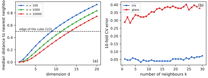
Figure 22.S7. (a) Exercise 22.10: the median distance from the centre of the cube to the nearest of \(n\) uniform points; the formula is exact while the median is below \(1/2\) (dashed). (b) Exercise 22.9: 10-fold cross-validation error of \(k\)-nearest neighbours (standardised covariates) for the iris and glass data. Code: fig_22_s7. Download: PDF · SVGExercise 22.11. Fit a tree to the spam data, then apply bagging.
Solution
On a random split into 3067 training and 1534 test messages, a single tree (deviance, R's stopping rules, 14 leaves) has test error 0.110. Bagging 60 such trees grown on bootstrap samples lowers it to 0.083 (Figure 22.S6(a)); most of the gain comes within the first ten trees. Averaging unstable trees reduces their variance; the bias of each tree is unchanged.
Exercise 22.12. Fit a tree with a single split to the spam data, then apply boosting.
Solution
On the same split, the best single stump (a split of the frequency of the character "$" at 0.0445) has test error 0.209. AdaBoost (Algorithm 22.C) with stumps reaches 0.095 after 10 rounds, 0.066 after 50, 0.063 after 100 and 0.059 after 200, with a minimum of 0.055; the training error keeps falling (0.037 after 400 rounds) while the test error flattens (Figure 22.S6(b)). Starting from a classifier far worse than one tree, boosting ends better than bagged trees: the bias reduction of Filling the gap 22.20 at work.
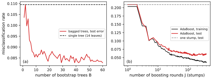
Figure 22.S6. Exercises 22.11 and 22.12 on the spam data (two thirds for training, one third for testing): (a) bagging trees; (b) AdaBoost with stumps, training and test error. Code: fig_22_s6,spam_results. Download: PDF · SVGExercise 22.13 (bias and variance in classification; Friedman 1997). Let \(\hh(x)=\ind\{\hr(x)\ge1/2\}\) and suppose \(\hr(x)\approx\N(\bar r(x),\sigma^2(x))\). Show that for fixed \(x\)
\[ \P(Y\ne\hh(x))\approx\P(Y\ne h^*(x))+|2r(x)-1|\Big\{1-\Phi\Big(\frac{\sgn(r(x)-\tfrac12)(\bar r(x)-\tfrac12)}{\sigma(x)}\Big)\Big\}, \]and discuss the implications. Hint: first show \(\P(Y\ne\hh(x))\)
\({}=|2r(x)-1|\,\P(\hh(x)\ne h^*(x))\) \({}+\P(Y\ne h^*(x))\). Solution
The hint. Here \(Y\) is a new response at \(x\), independent of the training data that determine \(\hh(x)\). Conditionally on \(\hh(x)\), Filling the gap 22.1 at the single point \(x\) gives \(\P(Y\ne\hh(x)\given\hh)-\P(Y\ne h^*(x))\)
\({}=|2r(x)-1|\ind\{\hh(x)\ne h^*(x)\}\); take expectations over the training data. The formula. If \(r(x)>1/2\), \(h^*(x)=1\) and \(\P(\hh\ne h^*)\)
\({}=\P(\hr<\tfrac12)\) \({}\approx\Phi\big((\tfrac12-\bar r)/\sigma\big)\) \({}=1-\Phi\big((\bar r-\tfrac12)/\sigma\big)\). If \(r(x)<1/2\), \(\P(\hh\ne h^*)\) \({}=\P(\hr\ge\tfrac12)\) \({}\approx1-\Phi\big((\tfrac12-\bar r)/\sigma\big)\). Both are \(1-\Phi\big(\sgn(r-\tfrac12)(\bar r-\tfrac12)/\sigma\big)\). (At \(r=1/2\) the extra term vanishes.) The formula agrees with a direct computation and with simulation. Implications. Call \(b(x)=\sgn(r-\tfrac12)(\bar r-\tfrac12)\) the boundary bias: positive when \(\hr\) is on average on the correct side of \(1/2\). Unlike squared error, bias and variance do not add. (1) If \(b>0\), the error falls as \(\sigma\) falls, and the size of the bias hardly matters: a badly biased \(\hr\) (say \(\bar r=0.55\) when \(r=0.95\)) classifies perfectly once its variance is small. (2) If \(b<0\), the estimate is on the wrong side on average and more variance helps, pushing the error towards a coin flip rather than certain failure. (3) Hence classification tolerates bias in \(\hr\) as long as it is on the right side of \(1/2\), and variance reduction is what matters: this is why crude probability estimates (naive Bayes, large-\(k\) neighbours, the linear regression of Section 22.4) often classify well (Figure 22.S8). See also Result 7.5 of Statistical Learning.
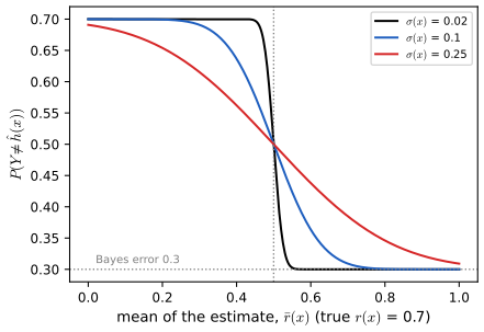
Figure 22.S8. Exercise 22.13 at a point with \(r(x)=0.7\): the probability of error of the plug-in rule against the mean \(\bar r\) of \(\hr\), for three standard deviations. On the correct side (\(\bar r>1/2\)) less variance is better whatever the bias; on the wrong side more variance is better. Code: fig_22_s8,friedman_error. Download: PDF · SVG
Demonstrations for this chapter
Each demonstration runs in the browser and links back to these notes. The ▶ Demo boxes above open them already set to the case under discussion.
| Demonstration | What you can see | Sections and results |
|---|---|---|
| The Bayes rule against LDA, QDA and logistic regression | Two simulated classes with known densities; the Bayes boundary and three fitted boundaries; the region where a fitted rule disagrees with the Bayes rule, and its exact excess risk; mean excess risk against \(n\). Presets: 1 equal covariances; 2 unequal covariances; 3 the same at \(n=20\); 4 unequal priors; 5 a far cluster (Section 22.5). | 22.2–22.5; Filling the gap 22.1, 22.7; Figure 22.S2 |
| How much does the training error flatter? Union and VC bounds | Empirical risk minimisation over unions of \(k\) intervals with a known \(r(x)\): training and true error, the exact largest deviation over the class, the union and VC bounds, and their coverage over 200 data sets. Presets: 1 two bumps, \(k=2\); 2 overfitting at \(k=20\); 3 pure noise; 4 \(n=5000\); 5 200 data sets. | 22.8; Theorems 22.17, 22.19; Filling the gaps 22.11–22.13; Figure 22.S3 |
| The hard-margin SVM through its dual | SMO step by step on small data sets: the boundary and margins of each iterate, the lower bound \(D(\alpha)\) and upper bound \(U(\alpha)\) closing on the optimum, the multipliers; kernels; click to remove points. Presets: 1 Figure 22.8; 2 five steps at a time; 3 Figure 22.9; 4 Exercise 22.7; 5 XOR with a Gaussian kernel. | 22.9, 22.10; Theorem 22.29; Filling the gap 22.16; Algorithm 22.A; Figure 22.S4 |
Related demonstrations: the Chapter 4 Hoeffding interval demo and the Chapter 13 logistic regression on the CORIS data; in the companion courses the LDA and QDA and SVM budget demos of Applied Statistical Learning, the SVM demo of Bayesian and Probabilistic Machine Learning, and the tree pruning, bagging and curse of dimensionality demos of Statistical Learning: Theory and Methods. The Python code that produces every figure of this page is code/ch22_classification.py (see the code index).
References
- Wasserman, L. (2004). All of Statistics: A Concise Course in Statistical Inference. Springer, New York. Chapter 22, pp. 349–379. www.stat.cmu.edu/~larry/all-of-statistics.
- Aronszajn, N. (1950). Theory of reproducing kernels. Transactions of the American Mathematical Society, 68(3), 337–404.
- Breiman, L. (1996). Bagging predictors. Machine Learning, 24(2), 123–140.
- Breiman, L., Friedman, J. H., Olshen, R. A. and Stone, C. J. (1984). Classification and Regression Trees. Wadsworth, Belmont.
- Cover, T. M. (1965). Geometrical and statistical properties of systems of linear inequalities with applications in pattern recognition. IEEE Transactions on Electronic Computers, 14(3), 326–334.
- Cover, T. M. and Hart, P. E. (1967). Nearest neighbor pattern classification. IEEE Transactions on Information Theory, 13(1), 21–27.
- Devroye, L., Györfi, L. and Lugosi, G. (1996). A Probabilistic Theory of Pattern Recognition. Springer, New York.
- Domingos, P. and Pazzani, M. (1997). On the optimality of the simple Bayesian classifier under zero-one loss. Machine Learning, 29(2–3), 103–130.
- Efron, B. (1975). The efficiency of logistic regression compared to normal discriminant analysis. Journal of the American Statistical Association, 70(352), 892–898.
- Fisher, R. A. (1936). The use of multiple measurements in taxonomic problems. Annals of Eugenics, 7(2), 179–188.
- Freund, Y. and Schapire, R. E. (1997). A decision-theoretic generalization of on-line learning and an application to boosting. Journal of Computer and System Sciences, 55(1), 119–139.
- Friedman, J. H. (1997). On bias, variance, 0/1-loss, and the curse-of-dimensionality. Data Mining and Knowledge Discovery, 1(1), 55–77.
- Hastie, T., Tibshirani, R. and Friedman, J. (2001). The Elements of Statistical Learning. Springer, New York.
- Herbrich, R. (2002). Learning Kernel Classifiers. MIT Press, Cambridge, MA.
- Keerthi, S. S., Shevade, S. K., Bhattacharyya, C. and Murthy, K. R. K. (2001). Improvements to Platt's SMO algorithm for SVM classifier design. Neural Computation, 13(3), 637–649.
- Mika, S., Rätsch, G., Weston, J., Schölkopf, B. and Müller, K.-R. (1999). Fisher discriminant analysis with kernels. In Neural Networks for Signal Processing IX, 41–48. IEEE.
- Platt, J. C. (1999). Fast training of support vector machines using sequential minimal optimization. In Advances in Kernel Methods: Support Vector Learning, 185–208. MIT Press.
- Rousseauw, J., du Plessis, J., Benade, A., Jordaan, P., Kotze, J., Jooste, P. and Ferreira, J. (1983). Coronary risk factor screening in three rural communities. South African Medical Journal, 64, 430–436.
- Sauer, N. (1972). On the density of families of sets. Journal of Combinatorial Theory, Series A, 13(1), 145–147.
- Schölkopf, B. and Smola, A. J. (2002). Learning with Kernels. MIT Press, Cambridge, MA.
- Shelah, S. (1972). A combinatorial problem; stability and order for models and theories in infinitary languages. Pacific Journal of Mathematics, 41(1), 247–261.
- Stone, C. J. (1977). Consistent nonparametric regression. The Annals of Statistics, 5(4), 595–620.
- Vapnik, V. N. (1998). Statistical Learning Theory. Wiley, New York.
- Vapnik, V. N. and Chervonenkis, A. Ya. (1971). On the uniform convergence of relative frequencies of events to their probabilities. Theory of Probability and its Applications, 16(2), 264–280.
Data sources: the CORIS, spam and glass data from the book's website (the spam data were collected at Hewlett-Packard Labs and are distributed with Hastie et al. 2001); the iris data of Fisher (1936), in the copy distributed with scikit-learn. The numerical statements in the text (the CORIS tables, trees and pruning sequence, the logistic and cross-validation errors of Figure 22.5, the excess-risk identity, the Fisher and LDA identities, the shatter counts and VC dimensions, Sauer's bound, the union-bound coverage, the SVM solutions and duality bounds, the kernel identities, the boosting bound and the solutions of the computational exercises) were confirmed numerically.