Learning with Fewer Labeled Examples
Models with millions of parameters are routinely trained on a few thousand labeled examples. This chapter collects the ways around that gap: manufacture more labeled data from the data at hand (augmentation, which is a smoothed empirical distribution), borrow structure from a larger task (transfer learning, adapters, self-supervised pre-training, the contrastive losses behind SimCLR and CLIP), exploit unlabeled inputs (self-training, entropy minimisation, label propagation, consistency regularisation, generative models), choose which labels to buy (active learning with the information gain and BALD), learn how to learn from a few examples (MAML, matching networks), and live with imprecise labels (soft labels, bags, distant supervision). The notes prove what the book leaves as "it can be shown": the vicinal-risk and variance-reduction arguments for augmentation, the InfoNCE lower bound on mutual information, the equivalence of soft self-training with EM, the harmonic solution of label propagation, virtual adversarial training as a power iteration, the submodularity behind batch active learning, and the sense in which a few gradient steps are a Gaussian prior. Small experiments check the claims.
Ch. 1 Introduction Ch. 2 Univariate probability Ch. 3 Multivariate probability Ch. 4 Statistics Ch. 5 Decision theory Ch. 6 Information theory Ch. 7 Linear algebra Ch. 8 Optimisation Ch. 9 Discriminant analysis Ch. 10 Logistic regression Ch. 11 Linear regression Ch. 12 GLMs Ch. 13 Networks for tabular data Ch. 14 Networks for images Ch. 15 Networks for sequences Ch. 16 Exemplar-based methods Ch. 17 Kernel methods Ch. 18 Trees and boosting Ch. 19 Fewer labels Ch. 20 Dimensionality reduction Ch. 21 Clustering Ch. 22 Recommender systems Ch. 23 Graph embeddings
How to read these notes
They follow the book. Sections carry the book's numbers (19.2.4.4, 19.3.2.2, ...) and equations that the book numbers keep their numbers, e.g. \((19.51)\); equations without a number are steps the book skips. The book does not mark any section of this chapter as optional except 19.3.6 (deep generative models), which is covered more briefly here.
Filling the gaps. Wherever the book writes "it can be shown", leaves a step to an exercise, or quotes a result from the literature, an orange Filling the gap box gives the full argument. Proofs start hidden: open one with its bar, or use the buttons below.
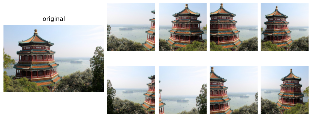
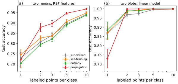
Figures and demonstrations. Every computed figure is reproduced by the Python code. Figures 19.1, 19.8, 19.9, 19.10 and 19.11 are reproduced; Figures 19.2 to 19.7, 19.12 to 19.16 (architecture and workflow diagrams) are hand-drawn sketches with nothing computed and are not reproduced. Original supplementary figures 19.S1 to 19.S10 test the claims proved here. Data: Figure 19.1 uses a photograph that ships with scikit-learn; Figures 19.8 to 19.10 and 19.S4, 19.S5 use simulated two-dimensional data; 19.S2 uses MNIST digits with added pixel noise. The book's own examples are illustrations without data; the captions say so. The ▶ Demo boxes open an interactive demonstration set to the case being discussed.
Main reference
K. P. Murphy, Probabilistic Machine Learning: An Introduction, MIT Press (2022), Chapter 19, pages 627–656 (book page: probml.github.io/pml-book/book1.html). Section, equation, figure and exercise numbers below refer to this book. The explanations, derivations, figures and code are my own.
Companion courses
Several of the ideas here are developed, in other notation, elsewhere on this site. Where a result is proved in full there, these notes give the statement and a short sketch and link to it.
- Foundations of Deep Learning (Bishop and Bishop): 9.1.3 symmetry and invariance (the other side of data augmentation), 9.3.1 early stopping, 19.1.4 denoising and 19.1.5 masked autoencoders (imputation tasks), 19.2 variational autoencoders, 17.1 adversarial training, the change of variables for flows, 12.1 attention.
- Bayesian and Probabilistic Machine Learning (Bishop): 9.2.2 EM for Gaussian mixtures and 9.3 the alternative view of EM (semi-supervised mixtures), 6.3.1 the Nadaraya-Watson model (matching networks), 10.1 variational inference.
- Elements of Statistical Learning: 6.6.2 kernel density classification, 14.3.7 Gaussian mixtures as soft K-means.
- Earlier chapters of this course: 6.3 mutual information, 5.1.1 Bayesian decision theory, 10.5 Bayesian logistic regression, 13.5 regularisation, 15.4.2 kernel regression as attention, 16.2.2 deep metric learning (the contrastive idea).
What this chapter adds: the vicinal-risk view of augmentation, adapters, the InfoNCE bound and the CLIP loss, the whole semi-supervised toolbox, BALD and batch active learning, MAML as a hierarchical-Bayes approximation, matching networks, and the treatment of weak labels.
The chapter at a glance
- 19.1 Augmentation replaces the empirical distribution by a smoothed one (gap 19.1); with symmetries of the data it is unbiased with smaller variance (gap 19.2).
- 19.2 Fine-tuning as MAP (gap 19.3), adapters (gap 19.4), the InfoNCE bound behind SimCLR (gap 19.5) and the CLIP loss and zero-shot rule (gap 19.6).
- 19.3 Self-training is EM when the labels are soft (gap 19.7); entropy minimisation selects low-density boundaries (gap 19.8) and maximises input-output mutual information (gap 19.9); label propagation has a harmonic solution (gap 19.10); consistency losses and virtual adversarial training (gap 19.11, gap 19.12); the semi-supervised VAE bound (gap 19.13); distillation (gap 19.14).
- 19.4 The value of information is non-negative (gap 19.15); information gain equals BALD (gap 19.16); greedy batch selection is within \(1-1/e\) (gap 19.17).
- 19.5–19.7 Gradient steps as a prior (gap 19.18), the MAML meta-gradient (gap 19.19), matching networks as kernel classifiers (gap 19.20), soft labels, label smoothing and noisy-OR bags (gap 19.21).
Notation. Labeled data \(\mathcal D_\ell=\{(\bm x_n,y_n)\}_{n=1}^{M}\), unlabeled inputs \(\mathcal D_u=\{\bm x_m\}_{m=1}^{N}\); \(p_\theta(y\given\bm x)\) is the model, \(\sigma\) the sigmoid, \(H(p)=-\sum_cp_c\log p_c\) the entropy in nats, \(a\) a logit, \(\mu_c=p_\theta(y=c\given\bm x)\). The mutual information is written \(\MI(\cdot;\cdot)\).
Prerequisites. Chapters 4 to 6 (estimation, MAP, information theory), 8 (optimisation), 10 (logistic regression and the Laplace approximation) and 13 to 15 (neural networks, convolutions, attention) of the book.
The chapter opens by noting that a 50-layer ResNet has about 23 million parameters, so that even with strongly correlated parameters a small labeled set invites overfitting, and the generic remedies of Section 13.5 (early stopping, weight decay, dropout) do not exhaust what can be done. p. 627
19.1 Data augmentation
p. 627 Data augmentation creates artificially modified copies of the training inputs that capture the variation expected at test time while keeping the label fixed. (In statistics the same words name the unrelated device of adding latent variables to speed up posterior simulation, a footnote of the book.)
19.1.1 Examples
p. 627 For images the standard transformations are random crops followed by resizing (a zoom), mirror flips and small colour changes (Figure 19.1); other modalities use background noise added to clean speech, random character or word replacement in text, or rendering synthetic text onto photographs. When one can afford to train many models, the best combination of transformations can itself be searched for with reinforcement learning or Bayesian optimisation (the AutoAugment family, Cubuk et al., 2019).
See also: Foundations of Deep Learning, Section 9.1.3 (symmetry and invariance).
19.1.2 Theoretical justification
p. 628 Augmentation seems to give something for nothing, but it injects prior knowledge: that the label does not change under the chosen transformations. In empirical risk minimisation the true risk \[ R(f)=\int \ell(f(\bm x),y)\,p^*(\bm x,y)\,\d\bm x\,\d y \tag{19.1} \] is approximated by replacing \(p^*\) with the empirical distribution \[ p_{\mathcal D}(\bm x,y)=\frac1N\sum_{n=1}^N\delta(\bm x-\bm x_n)\,\delta(y-y_n). \tag{19.2} \] Augmentation replaces it by the smoothed distribution \[ p_{\mathcal D}(\bm x,y\given\mathcal A)=\frac1N\sum_{n=1}^Np(\bm x\given\bm x_n,\mathcal A)\,\delta(y-y_n), \tag{19.3} \] where \(\mathcal A\) is the augmentation algorithm; the simplest example is \(p(\bm x\given\bm x_n,\mathcal A)=\N(\bm x\given\bm x_n,\sigma^2\bm I)\), a Parzen window in \(\bm x\) with a point mass in \(y\). Minimising the risk under (19.3) is vicinal risk minimisation (Chapelle et al., 2001): the risk is minimised in a neighbourhood of every training point. Two precise statements justify it.
Filling the gap 19.1: Gaussian-noise augmentation is a Tikhonov penalty p. 628, (19.3)
Derivation
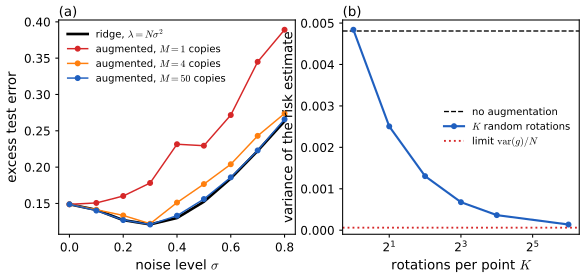
Let \(\ell(\bm x)=\ell(f(\bm x),y)\) be three times differentiable in \(\bm x\) with bounded derivatives and \(\bm\epsilon\sim\N(\bm 0,\sigma^2\bm I)\). Taylor's formula gives \[ \ell(\bm x+\bm\epsilon)=\ell(\bm x)+\nabla\ell^\T\bm\epsilon+\tfrac12\bm\epsilon^\T\nabla^2\ell\,\bm\epsilon+O(\|\bm\epsilon\|^3). \] The mean of \(\bm\epsilon\) is zero, \(\E[\bm\epsilon\bm\epsilon^\T]=\sigma^2\bm I\), and odd moments vanish, so the third-order term averages to zero and the remainder is \(O(\E\|\bm\epsilon\|^4)=O(\sigma^4)\): \[ \E_{\bm\epsilon}\,\ell(\bm x+\bm\epsilon)=\ell(\bm x)+\frac{\sigma^2}2\operatorname{tr}\nabla^2_{\bm x}\ell(\bm x)+O(\sigma^4). \] Squared loss, linear model. For \(\ell=(y-\bm w^\T\bm x)^2\), \(\nabla^2_{\bm x}\ell=2\bm w\bm w^\T\), and since \(\ell\) is quadratic the expansion is exact: \[ \E_{\bm\epsilon}(y-\bm w^\T(\bm x+\bm\epsilon))^2=(y-\bm w^\T\bm x)^2+\sigma^2\|\bm w\|^2 . \] Summing over the \(N\) training points, the augmented risk is the ridge objective \(\sum_n(y_n-\bm w^\T\bm x_n)^2+N\sigma^2\|\bm w\|^2\) with \(\lambda=N\sigma^2\), minimised by \(\hat{\bm w}=(\bm X^\T\bm X+N\sigma^2\bm I)^{-1}\bm X^\T\bm y\). Least squares on \(M\) independent noisy copies of the data converges to this solution as \(M\to\infty\) by the law of large numbers (the normal equations are averages of i.i.d. terms with this expectation). Figure 19.S1a shows the excess test error of the augmented fit approaching the ridge curve as \(M\) grows.
Logistic loss. For \(\ell=\operatorname{softplus}(-\tilde y\,\bm w^\T\bm x)\) the Hessian in \(\bm x\) is \(\sigma'(a)\,\bm w\bm w^\T\) with \(a=\bm w^\T\bm x\), so the induced penalty is \(\frac{\sigma^2}2\|\bm w\|^2\sigma(a)(1-\sigma(a))\): an input-dependent weight decay that is largest for points near the boundary (\(a\approx0\)) and negligible for confidently classified ones. For squared loss on a linear model the noise is thus the same as an \(\ell_2\) penalty (Section 4.5.3, Bishop, 1995); for nonlinear \(f\) the penalty also involves the curvature of the network in its input. \(\square\)
Filling the gap 19.2: augmentation under an invariance is unbiased and has lower variance p. 628
Proof
Suppose \(\mathcal A\) draws a transformation \(t\sim Q\) and returns \((t(\bm x),y)\), and that the data distribution is invariant: for every \(t\) in the support of \(Q\), \((t(\bm x),y)\) has the same distribution as \((\bm x,y)\) when \((\bm x,y)\sim p^*\). (A rotation of a texture, a mirror flip of a cat photograph.) Let \(\ell_t=\ell(f(t(\bm x)),y)\) and \(g(\bm x,y)=\E_{t\sim Q}\,\ell_t\).
Unbiasedness. For each fixed \(t\), \(\E\,\ell_t=R(f)\) by invariance, so \(\E\,g=\E_t\E\,\ell_t=R(f)\). The augmented empirical risk \(\hat R_{\rm aug}=\frac1N\sum_ng(\bm x_n,y_n)\) has the same mean as the plain one, \(R(f)\), when the invariance is true.
Variance. By invariance all \(\ell_t\) have the same variance \(v=\var(\ell)\), and \(g\) is their average over \(t\). The standard deviation is a norm, so by the triangle inequality \(\operatorname{sd}(g)\le\E_t\operatorname{sd}(\ell_t)=\sqrt v\). Hence \(\var(\hat R_{\rm aug})=\var(g)/N\le\var(\hat R)=v/N\).
With \(K\) sampled transformations per point, the law of total variance gives \(\var(\hat R_K)=\frac1N\big[\var(g)+\E\,\var_t(\ell_t\given\bm x,y)/K\big]\): the variance falls like \(1/K\) towards the floor \(\var(g)/N\). Figure 19.S1b: for a fixed non-invariant classifier on a rotation-invariant two-dimensional data set (\(N=50\)), the variance of the 0-1 risk estimate is \(5.1\times10^{-3}\) without augmentation, \(5.1\times10^{-3}\) with \(K=1\) (one random rotation is just another draw from \(p^*\), no gain), \(1.4\times10^{-4}\) with \(K=64\), against a floor of \(6.0\times10^{-5}\).
If the invariance is false the augmented risk is a biased estimate of \(R(f)\): the bias is \(\E_t\E\,\ell_t-R(f)\), which is the price of the prior knowledge; the benefit is the variance reduction above and, for flexible \(f\), the restriction to functions that vary slowly along the transformations. \(\square\)
19.2 Transfer learning
pp. 628–629 Many data-poor tasks resemble data-rich ones: fine-grained classification of endangered birds is helped by training first on all birds. Transfer learning trains a model with parameters \(\theta\) on a large source set \(\mathcal D_p\) (pre-training, labeled or not) and then continues on the small labeled target set \(\mathcal D_q\) (fine-tuning).
19.2.1 Fine-tuning
pp. 629–630 Suppose a pre-trained classifier \(p(y\given\bm x,\theta_p)=\softmax(\bm W_2\bm h(\bm x;\theta_1)+\bm b_2)\) works for inputs \(\mathcal X_p\) and outputs \(\mathcal Y_p\), and we want \(q(y\given\bm x,\theta_q)\) for a new label set \(\mathcal Y_q\) on similar inputs. Output sets usually differ, so the final layer is cut off and replaced by a new head: \[ q(y\given\bm x,\theta_q)=\softmax(\bm W_3\bm h(\bm x;\theta_1)+\bm b_3),\qquad\theta_q=(\bm W_3,\bm b_3,\theta_1), \] with the feature extractor \(\bm h\) shared. If \(\theta_1\) is frozen the model is linear in its remaining parameters and fitting it is convex; if \(\theta_1\) is also updated, a small learning rate keeps it near the pre-trained value. When the input domains differ, domain adaptation (Section 19.2.5) is needed.
Filling the gap 19.3: why a frozen trunk is convex, and why a small learning rate or a penalty keeps the trunk near \(\theta_p\) pp. 629–630
Derivation
Convexity. With \(\bm h_n=\bm h(\bm x_n;\theta_1)\) fixed, the negative log-likelihood in \((\bm W_3,\bm b_3)\) is that of multinomial logistic regression with inputs \(\bm h_n\) (Chapter 10), \(-\sum_n\log\mu_{n,y_n}\), \(\bm\mu_n=\softmax(\bm W_3^\T\bm h_n+\bm b_3)\). Its Hessian is \(\sum_n(\diag\bm\mu_n-\bm\mu_n\bm\mu_n^\T)\otimes\bm h_n\bm h_n^\T\) (gap 10.9). For any vector \(\bm v\), \(\bm v^\T(\diag\bm\mu-\bm\mu\bm\mu^\T)\bm v=\var_{c\sim\bm\mu}(v_c)\ge0\), and a Kronecker product of positive semi-definite matrices is positive semi-definite, so the Hessian is positive semi-definite and the problem is convex (strictly, after fixing one class's weights to zero and if the features have full rank). Hence a simple solver such as IRLS (Section 10.2.6) converges to the global optimum, which is useful in the long-tail regime of few labels per class.
Staying near \(\theta_p\). Minimising \(\mathcal L(\theta)+\frac\lambda2\|\theta-\theta_p\|^2\) is MAP estimation with the Gaussian prior \(\N(\theta_p,\lambda^{-1}\bm I)\) centred at the pre-trained weights (add the log-prior \(-\frac\lambda2\|\theta-\theta_p\|^2\) to the log-likelihood). For a quadratic \(\mathcal L(\theta)=\frac12\|\bm y-\bm X\theta\|^2\) the minimiser is \(\hat\theta=(\bm X^\T\bm X+\lambda\bm I)^{-1}(\bm X^\T\bm y+\lambda\theta_p)\) (set the gradient to zero), a ridge estimate shrunk towards \(\theta_p\) instead of \(\bm 0\). A small learning rate with a small number of gradient steps from \(\theta_p\) achieves a similar effect: gap 19.18 shows that \(K\) gradient steps from \(\theta_p\) on a quadratic loss equal the MAP estimate with a Gaussian prior centred at \(\theta_p\), whose strength falls as \(K\) grows. \(\square\)
See also: Chapter 10, Section 10.3 (multinomial logistic regression); Foundations of Deep Learning, 9.3.1 (early stopping).
19.2.2 Adapters
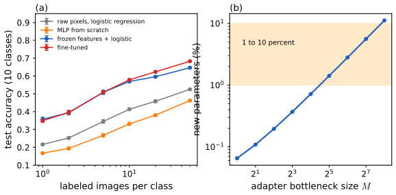
pp. 630–631 Fine-tuning every parameter is slow and needs one full model per task. Adapters keep the pre-trained network untouched and add a few new parameters inside it. For a transformer (Houlsby et al., 2019) two shallow bottleneck MLPs with skip connections are inserted in each layer, one after the attention block and one after the feed-forward block; with feature size \(D\) and bottleneck \(M\) each adds \(O(DM)\) parameters. Only the adapters, the layer-norm parameters and the output head are trained; typically 1 to 10 percent of the original parameter count suffices. For a residual network (Rebuffi et al., 2017, 2018) a \(1\times1\) convolution \(\bm\alpha\in\R^{C\times D}\) acts on the channels after a convolution \(f\); in series \[ \rho(\bm x)=\bm x+\operatorname{diag}_1(\bm\alpha)\circledast\bm x=\operatorname{diag}_1(\bm I+\bm\alpha)\circledast\bm x, \tag{19.4} \] \[ \bm y=\rho(f\circledast\bm x)=\big(\operatorname{diag}_1(\bm I+\bm\alpha)\circledast f\big)\circledast\bm x, \tag{19.5} \] or in parallel \[ \bm y=f\circledast\bm x+\operatorname{diag}_1(\bm\alpha)\circledast\bm x=\big(f+\operatorname{diag}_L(\bm\alpha)\big)\circledast\bm x, \tag{19.6} \] with \(\bm\alpha=\bm 0\) giving the identity at initialisation and \(O(C^2)\) parameters per layer.
Filling the gap 19.4: the adapter algebra (19.4)–(19.6) and the parameter count pp. 630–631
Derivation
Convolution is linear in the filter and in the input. Write the filter as a tensor \(F[u,v,c,d]\) (spatial offsets \(u,v\), input channel \(c\), output channel \(d\)), so \((f\circledast\bm x)_d=\sum_{c,u,v}F[u,v,c,d]\,x_c(\cdot+(u,v))\).
Series adapter (19.5). A \(1\times1\) convolution with matrix \(\bm A=\bm I+\bm\alpha\) mixes output channels: \(z_e=\sum_dA_{de}\,y_d\). Substituting \(y_d\) and exchanging the order of the finite sums, \(z_e=\sum_{c,u,v}\big(\sum_dA_{de}F[u,v,c,d]\big)x_c(\cdot+(u,v))\), i.e. \(\bm z=f'\circledast\bm x\) with \(F'[u,v,c,e]=\sum_dA_{de}F[u,v,c,d]\): the adapter is a re-mixing of the output channels of the filter. At \(\bm\alpha=\bm 0\), \(\bm A=\bm I\) and \(F'=F\). The book calls this a "low-rank multiplicative perturbation": it acts through the \(D\times D\) matrix \(\bm\alpha\) on one mode of the filter tensor, and it is low rank only if \(\bm\alpha\) is constrained to be (the book's \(\bm\alpha\) is an unconstrained matrix).
Parallel adapter (19.6). Take odd kernel size \(k\), same padding and \(C_{\rm in}=D\). A \(1\times1\) convolution of \(\bm x\) is a convolution whose filter is non-zero only at the centre offset \((0,0)\): \(\operatorname{diag}_L(\bm\alpha)[u,v,c,d]=\alpha_{cd}\,\ind(u=v=0)\). By linearity in the filter, \(f\circledast\bm x+\operatorname{diag}_1(\bm\alpha)\circledast\bm x=(F+\operatorname{diag}_L(\bm\alpha))\circledast\bm x\): an additive perturbation of the centre tap only.
Counts. A transformer adapter is \(\bm x\mapsto\bm x+\bm W_{\rm up}\,\phi(\bm W_{\rm down}\bm x+\bm b_d)+\bm b_u\) with \(\bm W_{\rm down}\in\R^{M\times D}\): \(2DM+D+M\) parameters, and setting \(\bm W_{\rm up}=\bm 0\) gives the identity through the skip connection. Two per layer give \(2(2DM+D+M)\approx4DM\). A transformer layer has about \(12D^2\) parameters (\(4D^2\) in the attention projections and \(8D^2\) in a feed-forward block with hidden size \(4D\)), so adapters add a fraction \(\approx M/(3D)\) of the layer: with \(D=768\) and \(M=64\), 2.8 percent, inside the 1 to 10 percent range of the book (Figure 19.S2b). For the convolutional adapter, \(D^2\) new parameters per layer compare with \(k^2C_{\rm in}D\) in the filter: a fraction \(1/(k^2)\) for \(C_{\rm in}=D\). All four identities (series, parallel, identity at zero, counts) were also confirmed numerically on random filters. \(\square\)
19.2.3 Supervised pre-training
pp. 631–632 The pre-training task may be supervised or not; what matters is that it teaches structure that the downstream task needs and is sufficiently similar to it. The standard example is ImageNet (1.28 million images, 1000 classes) for CNNs. The benefit shrinks when the target domain differs strongly (medical images), and for object detection it is often only a speed-up, a warm start of the optimiser from which training from scratch eventually catches up. Outside vision, supervised pre-training is rarer; examples are natural language inference data for sentence embeddings and a large English corpus for low-resource speech recognition.
19.2.4 Unsupervised pre-training (self-supervised learning)
p. 632 Unlabeled data are cheap, so pre-training increasingly uses them. When the labels are manufactured from the data themselves the task is called self-supervised. (An older practice, unsupervised pre-training of a network on the labeled set itself, ignoring the labels, is different from the transfer setting here.) Self-supervised tasks are discriminative, predicting outputs from inputs, unlike the generative models of Chapter 20. Three families are distinguished.
19.2.4.1 Imputation tasks
p. 632 Split the input \(\bm x=(\bm x_h,\bm x_v)\) into a hidden and a visible part and predict \(\hat{\bm x}_h=f(\bm x_v,\bm x_h=\bm 0)\): a fill-in-the-blank or cloze task (Figure 19.4, a diagram). Masked language models and masked autoencoders are instances.
See also: Foundations of Deep Learning, 19.1.4 (denoising autoencoders) and 19.1.5 (masked autoencoders).
19.2.4.2 Proxy tasks
p. 633 Proxy (pretext) tasks build pairs \((\bm x_1,\bm x_2)\), for instance \(\bm x_2=t(\bm x_1)\) with \(t\) a transformation under our control, and train a Siamese network \(p(y\given\bm x_1,\bm x_2)=p(y\given r[f(\bm x_1),f(\bm x_2)])\) to predict a label \(y\) describing the relation, for example the rotation angle used. The representation \(f\) is what is kept for downstream tasks.
19.2.4.3 Contrastive tasks
p. 633 The most popular family builds pairs of semantically similar examples by augmentation (Section 19.1) and trains the embedding to put them closer together than two unrelated examples. This is the idea of deep metric learning (Section 16.2.2) with self-generated similar pairs.
19.2.4.4 SimCLR
pp. 633–635 SimCLR (Chen et al., 2020) turns an input \(\bm x\) into two augmented views \(\bm x_1=t_1(\bm x)\), \(\bm x_2=t_2(\bm x)\) and takes the other examples of the minibatch as negatives \(\bm x^-_1,\dots,\bm x^-_n\in\mathcal N(\bm x)\); with a feature map \(F:\R^D\to\R^E\) it maximises \[ J=F(t_1(\bm x))^\T F(t_2(\bm x))-\log\sum_{\bm x^-_i\in\mathcal N(\bm x)}\exp\big(F(\bm x^-_i)^\T F(t_1(\bm x))\big) \tag{19.7} \] (in practice with unit-norm embeddings, i.e. cosine similarity, and a temperature). The same idea is a conditional energy-based model \[ p(\bm x_2\given\bm x_1)=\frac{\exp[-E(\bm x_2\given\bm x_1)]}{Z(\bm x_1)},\quad E(\bm x_2\given\bm x_1)=-F(\bm x_2)^\T F(\bm x_1), \tag{19.8} \] \[ Z(\bm x)=\int\exp[-E(\bm x^-\given\bm x)]\,\d\bm x^-=\int\exp[F(\bm x^-)^\T F(\bm x)]\,\d\bm x^-, \tag{19.9} \] with conditional log-likelihood \[ \log p(\bm x_2\given\bm x_1)=F(\bm x_2)^\T F(\bm x_1)-\log\int\exp[F(\bm x^-)^\T F(\bm x_1)]\,\d\bm x^-, \tag{19.10} \] and (19.7) replaces the integral by a Monte Carlo sum over the negatives. Random crops force the network to predict a local view from a global one and to relate adjacent views; a random colour distortion is added because positives and negatives are otherwise distinguishable by colour histograms alone. SimCLR needs large batches for enough diverse negatives; a memory bank of past embeddings updated by an exponential moving average (MoCo, He et al., 2020) is the alternative.
Filling the gap 19.5: the InfoNCE bound \(\MI(X;Y)\ge\log N-L_N\), and in which sense (19.7) bounds the likelihood pp. 634–635, (19.7)–(19.10)
Proof
Result 19.1 (van den Oord et al., 2018; Poole et al., 2019). Let \((\bm x_i,y_i)\), \(i=1,\dots,N\), be i.i.d. from \(p(\bm x,y)\) and \(f(\bm x,y)\) any real critic (the score \(F(\cdot)^\T F(\cdot)\) of the book). Define the InfoNCE loss \[ L_N=-\E\log\frac{e^{f(\bm x_1,y_1)}}{\sum_{j=1}^Ne^{f(\bm x_1,y_j)}} . \] Then \(\MI(X;Y)\ge\log N-L_N\). Consequently the estimate can never exceed \(\log N\).
Proof. (i) A variational bound. For any function \(g\) and any pair of distributions \(P\ll Q\) with \(u=\d P/\d Q\), the pointwise inequality \(u\log u\ge ug-e^{g-1}\) holds for \(u\ge0\) (the right side, as a function of \(g\), is maximised at \(g=1+\log u\) where it equals \(u\log u\)). Integrating against \(Q\) gives \(\KL(P\|Q)\ge\E_Pg-\E_Qe^{g-1}\). Take \(P=p(\bm x,y)\), \(Q=p(\bm x)p(y)\), so that \(\KL(P\|Q)=\MI(X;Y)\).
(ii) A baseline. Fix the context \(c=(y_2,\dots,y_N)\), independent of \((\bm x_1,y_1)\) under both \(P\) and \(Q\). Apply (i) conditionally on \(c\) with \[ g(\bm x,y)=1+f(\bm x,y)-\log a(\bm x,y;c),\qquad a(\bm x,y;c)=\frac1N\Big(e^{f(\bm x,y)}+\sum_{j\ge2}e^{f(\bm x,y_j)}\Big). \] Then \(\E_Pg-\E_Qe^{g-1}=1+\E_P[f-\log a]-\E_Q[e^{f(\bm x,y)}/a]\).
(iii) The second term is exactly 1. Under \(Q\), \(\bm x\) is independent of \(y,y_2,\dots,y_N\), which are i.i.d. \(p(y)\), hence exchangeable given \(\bm x\); write \(y_1:=y\). Then \(\E[e^{f(\bm x,y_1)}/a]=\frac1N\sum_{j}\E[e^{f(\bm x,y_j)}/a]=\E[\frac1N\sum_je^{f(\bm x,y_j)}/a]=\E[1]=1\).
(iv) Combining, averaging over \(c\), \(\MI(X;Y)\ge\E\log\frac{e^{f(\bm x_1,y_1)}}{a}=\E\log\frac{N\,e^{f(\bm x_1,y_1)}}{\sum_je^{f(\bm x_1,y_j)}}=\log N-L_N\). \(\square\)
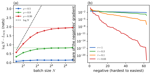
Remarks. (a) The bound is tight, as \(N\to\infty\), for the optimal critic \(f^*(\bm x,y)=\log\frac{p(y\given\bm x)}{p(y)}+c(\bm x)\); Figure 19.S3a shows \(\log N-L_N\) for a bivariate Gaussian pair with correlation \(\rho\), for which \(\MI=-\frac12\log(1-\rho^2)\) and \(f^*\) is known in closed form: with \(N=512\) and \(\rho=0.9\) the estimate is 0.827 against the true 0.830, but for \(\rho=0.99\) the bound is capped by \(\log N\) until \(N\) exceeds \(e^{\MI}\approx7\). This is the quantitative reason why contrastive methods need many negatives. (b) Relation to (19.10). Let \(\hat Z\) be the Monte Carlo sum over the negatives, an unbiased estimate of \(Z\) up to the sampling distribution. By Jensen's inequality \(\E\log\hat Z\le\log\E\hat Z=\log Z\), so \(\E J=\E[s^+-\log\hat Z]\ge s^+-\log Z\): in expectation (19.7) is an upper bound on the conditional log-likelihood (19.10), which is the sense of the book's "Monte Carlo upper bound". It is therefore not a lower bound on the likelihood; the mutual-information bound above is the cleaner justification. \(\square\)
See also: Chapter 6, Section 6.3 (mutual information); Section 16.2.2 (deep metric learning).
19.2.4.5 CLIP
pp. 635–637 CLIP (Radford et al., 2021) is contrastive learning between two modalities on about 400 million (image, text) pairs from the web. For a minibatch of \(N\) pairs, let \(\bm I_i=f_I(\bm x_i)/\|f_I(\bm x_i)\|\) and \(\bm T_j=f_T(y_j)/\|f_T(y_j)\|\) be the unit-norm image and text embeddings, and \[ L_{ij}=\bm I_i^\T\bm T_j \tag{19.11} \] the matrix of logits. The loss, an average of the two cross entropies of "which text goes with image \(i\)" and "which image goes with text \(j\)", is \[ J=\frac12\Big(\sum_{i=1}^N\operatorname{CE}(\bm L_{i,:},\bm 1_i)+\sum_{j=1}^N\operatorname{CE}(\bm L_{:,j},\bm 1_j)\Big),\qquad\operatorname{CE}(\bm p,\bm q)=-\sum_{k=1}^Kp_k\log q_k, \tag{19.12, 19.13} \] where the logits are in practice multiplied by a learned inverse temperature. With a ResNet or vision transformer for \(f_I\), a text transformer for \(f_T\) and \(N\approx32\)k the model is trained for days on hundreds of accelerators. At test time zero-shot classification converts each of the \(K\) class names into a sentence \(y_k\) ("a photo of a dog"), embeds it, and computes \[ p(y=k\given\bm x)=\softmax\big([\bm I^\T\bm T_1,\dots,\bm I^\T\bm T_K]\big)_k . \tag{19.14} \] This can match supervised ImageNet accuracy without any ImageNet label, although the images come from the web and similar data were seen. The method is sensitive to the wording of the class prompt ("a photo of guacamole, a type of food"); adding such phrases by hand is prompt engineering. (As printed, (19.12) is a sum; to be an average over the minibatch, as the text says, it carries a factor \(1/N\).)
Filling the gap 19.6: the CLIP gradient, the role of the temperature, and zero-shot classification as a Bayes rule pp. 636–637, (19.12), (19.14)
Derivation
Gradient. Row \(i\) of the loss is \(-L_{ii}+\operatorname{lse}(\bm L_{i,:})\) and \(\partial\operatorname{lse}(\bm L_{i,:})/\partial L_{ij}=\softmax(\bm L_{i,:})_j=:r_{ij}\); column \(j\) is analogous with \(c_{ij}=\softmax(\bm L_{:,j})_i\). Hence, with the \(1/N\) of the average, \[ \frac{\partial J}{\partial L_{ij}}=\frac1{2N}\big(r_{ij}+c_{ij}-2\,\delta_{ij}\big). \] The positive pair is pushed up with weight \(1-\frac12(r_{ii}+c_{ii})\) and each negative is pushed down with weight proportional to its softmax probability. With a temperature, \(L_{ij}=s_{ij}/\tau\) for cosine similarity \(s_{ij}\), the weights are \(\softmax(\bm s_{i,:}/\tau)_j\): as \(\tau\to\infty\) every negative has weight \(1/N\); as \(\tau\to0\) the mass collapses onto the hardest (most similar) negative, \(\arg\max_{j\ne i}s_{ij}\) (Figure 19.S3b: the five hardest of 63 negatives carry 14 percent of the gradient at \(\tau=1\), 38 percent at 0.3, 92 percent at 0.1 and 100 percent at 0.03).
Zero-shot as a Bayes classifier. Model each class \(k\) as a von Mises–Fisher density on the unit sphere with direction \(\bm T_k\) and concentration \(\kappa=1/\tau\): \(p(\bm I\given k)=C_d(\kappa)\exp(\kappa\bm T_k^\T\bm I)\), where the normaliser \(C_d(\kappa)\) does not depend on \(\bm T_k\) (rotate the sphere). With equal class priors, Bayes' rule gives \(p(k\given\bm I)=\exp(\kappa\bm T_k^\T\bm I)/\sum_{k'}\exp(\kappa\bm T_{k'}^\T\bm I)\), which is (19.14) with the logits scaled by \(\kappa\). So the learned temperature is the concentration of the class-conditional densities, and the zero-shot rule is the Bayes-optimal rule for that model (confirmed numerically on the sphere in three dimensions with the closed-form normaliser \(\kappa/(4\pi\sinh\kappa)\)). \(\square\)
See also: Foundations of Deep Learning, 12.4.5 (vision and language transformers).
19.2.5 Domain adaptation
p. 637 In domain adaptation the inputs come from a source domain \(\mathcal X_s\) and a target domain \(\mathcal X_t\) with the same labels \(\mathcal Y\), and there are no labeled target examples (the "dual" of transfer learning). Domain-adversarial learning (Ganin et al., 2016) trains the classifier so that it cannot tell which domain an input came from, so that it uses only features common to both. With domain label \(d_n\in\{s,t\}\), feature map \(f_\theta\) and classifier head \(g_\phi\) the objective is \[ \min_\phi\max_\theta\ \frac1{N_s+N_t}\sum_{n\in\mathcal D_s,\mathcal D_t}\ell(d_n,f_\theta(\bm x_n))+\frac1{N_s}\sum_{m\in\mathcal D_s}\ell(y_m,g_\phi(f_\theta(\bm x_m))) , \tag{19.15} \] implemented by a gradient-sign-reversal layer and related to GANs (Chapter 17 of the Bishop and Bishop course). The first term is a domain classifier loss that the features try to maximise; the second is the ordinary task loss on source labels.
19.3 Semi-supervised learning
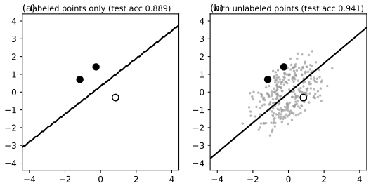
p. 638 Labels are often expensive: transcribing speech takes many times real time, and medical labels need experts. Semi-supervised learning assumes that, besides samples \((\bm x,y)\sim p(\bm x,y)\), we have many more samples \(\bm x\sim p(\bm x)\) of the inputs alone (Figure 19.8). The unlabeled data tell us about the high-level structure of \(p(\bm x)\), and the labeled data only the fine detail of the task.
19.3.1 Self-training and pseudo-labeling
pp. 638–639 In self-training (Scudder, 1965) the model predicts labels for the unlabeled data and these pseudo-labels (Lee, 2013) are used as if they were true. The offline variant predicts for all unlabeled points, refits (possibly from scratch) on labeled plus pseudo-labeled data, and repeats; the online variant keeps predicting on random unlabeled batches and trains on them at once. Offline training uses stale pseudo-labels, online training pays for constant relabeling. The danger is confirmation bias (Tarvainen and Valpola, 2017): wrong predictions are fed back as labels, so the model grows more confident in its mistakes. A selection metric keeps only pseudo-labels that are probably right, typically those whose largest class probability exceeds a threshold \(\tau\) (useful only if the probabilities are calibrated).
Filling the gap 19.7: loss gradients of self-training and entropy minimisation, and self-training with soft labels is EM pp. 638–640, (19.16), (19.17), p. 640
Derivation
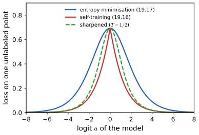
Gradients in the binary case. Let \(a\) be the logit and \(p=\sigma(a)\). The entropy is \(H(a)=\operatorname{softplus}(a)-a\sigma(a)\) and \[ \frac{\d H}{\d a}=\frac{\d H}{\d p}\frac{\d p}{\d a}=\log\frac{1-p}{p}\cdot p(1-p)=-a\,p(1-p). \] The online self-training loss (19.16), \(-\max_c\log p_c\), equals \(\operatorname{softplus}(-|a|)\) with derivative \(-\operatorname{sign}(a)\,\sigma(-|a|)\). Both push \(|a|\) up and both are \(\log2\) at \(a=0\) (Figure 19.9), but entropy minimisation has zero gradient at \(a=0\) (an unstable stationary point) whereas hard self-training has the non-zero slopes \(\mp\frac12\) on either side: the hard target breaks the tie abruptly.
Sharpening. Raising the probabilities to the power \(1/T\) and renormalising gives \(q_T(\bm p)\). As \(T\to0\) it tends to the one-hot argmax (hard self-training); at \(T=1\) it is \(\bm p\) itself. The book says that at \(T=1\) the cross entropy with this target "is equivalent to entropy minimisation". As a loss value it is: \(\operatorname{CE}(\bm p,\bm p)=H(\bm p)\). As a training signal it is not, if the target is treated as a constant, which is how the targets are used in practice: the gradient of \(-\sum_cq_c\log p_c\) with respect to the logits is \(\bm p-\bm q\), which vanishes when \(\bm q=\bm p\), whereas the gradient of \(H(\bm p)\) is not zero (above). Fixing the target at \(T=1\) therefore provides no signal from the unlabeled data; a sharpening temperature \(T<1\) is what produces one (confirmed numerically: at \(a=0.9\) the fixed-target gradient is \(10^{-11}\), the entropy gradient \(-0.185\)).
Self-training with soft labels is EM. Take a generative classifier \(p(\bm x,y\given\theta)=\pi_yp(\bm x\given\phi_y)\) (a Gaussian mixture, say). The log-likelihood of labeled and unlabeled data is \[ \ell(\theta)=\sum_{n\in\mathcal D_\ell}\log p(\bm x_n,y_n\given\theta)+\sum_{m\in\mathcal D_u}\log\sum_yp(\bm x_m,y\given\theta). \] EM (Chapter 9 of the Bishop course) sets \(r_{my}=p(y\given\bm x_m,\theta_t)\), the current model's soft pseudo-labels, and maximises \[ Q(\theta\given\theta_t)=\sum_{n\in\mathcal D_\ell}\log p(\bm x_n,y_n\given\theta)+\sum_{m\in\mathcal D_u}\sum_yr_{my}\log p(\bm x_m,y\given\theta), \] i.e. a weighted maximum-likelihood refit on labeled and soft-pseudo-labeled data: one round of self-training with soft targets (and no threshold, \(\tau\le1/2\)). The likelihood never decreases: \(\ell(\theta)\ge Q(\theta\given\theta_t)+\sum_mH(\bm r_m)\) for all \(\theta\) by Jensen's inequality, with equality at \(\theta=\theta_t\); maximising \(Q\) therefore gives \(\ell(\theta_{t+1})\ge Q(\theta_{t+1}\given\theta_t)+\sum_mH(\bm r_m)\ge Q(\theta_t\given\theta_t)+\sum_mH(\bm r_m)=\ell(\theta_t)\). Hard pseudo-labels (argmax) give classification EM, which has no such guarantee. For a discriminative classifier such as logistic regression neither guarantee holds, which is why confirmation bias can occur (Figure 19.S4 and the demo). The monotone increase of \(\ell\) was confirmed numerically for shared and for separate covariances, and the M step reproduced as a weighted refit. \(\square\)
19.3.2 Entropy minimization
pp. 639–640 Self-training implicitly pushes the model towards confident predictions. With the online cross-entropy loss on unlabeled data this is explicit: \[ \mathcal L=-\max_c\log p_\theta(y=c\given\bm x), \tag{19.16} \] minimised when all probability sits on one class. Entropy minimisation (Grandvalet and Bengio, 2005) uses the entropy itself, \[ \mathcal L=-\sum_{c=1}^Cp_\theta(y=c\given\bm x)\log p_\theta(y=c\given\bm x). \tag{19.17} \] The two differ in the target: (19.16) is the cross entropy to the hard target \(\arg\max p_\theta\), (19.17) to the soft target \(p_\theta\); the temperature interpolates between them (MixMatch). Figure 19.9 compares the three losses for a binary problem.
19.3.2.1 The cluster assumption
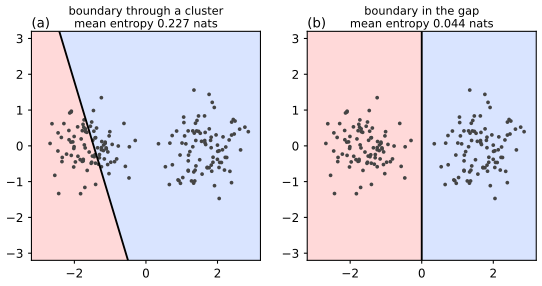
pp. 640–641 Many semi-supervised methods assume that the classes form clusters, so that the decision boundary should run through a low-density region of the data. If the model is smooth, a boundary through a dense region forces high-entropy predictions for many data points; minimising the entropy therefore moves the boundary into the gaps (Figure 19.10).
Filling the gap 19.8: what entropy minimisation actually does, the entropy is proportional to the density at the boundary pp. 640–641
Derivation
It is degenerate without a size constraint. Let \(a(\bm x)=\kappa(\bm w^\T\bm x+b)\) with \(\|\bm w\|=1\) and suppose the data distribution gives zero mass to the boundary. For \(t\ne0\), \(H(\sigma(\kappa t))\to0\) as \(\kappa\to\infty\) and \(0\le H\le\log2\), so by dominated convergence the mean entropy \(\E\,H(\sigma(a(\bm x)))\to0\) for every boundary. So (19.17) alone is minimised by making the classifier arbitrarily sharp, wherever the boundary is; its guidance comes only through the trade-off with the labeled-data loss and a penalty on the weights (Figure 19.10 holds the weight norm fixed). Numerically (two clusters, boundary through the left one): mean entropy 0.433, 0.120, 0.018, 0.0017 for \(\kappa=1,10,100,1000\).
At finite sharpness the entropy measures the density at the boundary. In one dimension let \(x\) have a continuous density \(p\), the boundary be at \(c\) and \(a=\kappa(x-c)\). The substitution \(u=\kappa(x-c)\) gives \[ \E\,H(\sigma(a))=\int p(x)H(\sigma(\kappa(x-c)))\,\d x=\frac1\kappa\int p\Big(c+\frac u\kappa\Big)H(\sigma(u))\,\d u\ \sim\ \frac{p(c)}\kappa\int_{-\infty}^{\infty}H(\sigma(u))\,\d u=\frac{\pi^2}3\,\frac{p(c)}\kappa , \] as \(\kappa\to\infty\): continuity of \(p\) and the exponential decay of \(H(\sigma(u))\) justify dominated convergence, and \(\int_{-\infty}^\infty H(\sigma(u))\d u=\pi^2/3\) (evaluated numerically to 8 digits; analytically, \(H(\sigma(u))=\operatorname{softplus}(u)-u\sigma(u)\), and the integral over \(u>0\) of \(\log(1+e^{-u})+u\sigma(-u)\) is \(\pi^2/12+\pi^2/12\), twice by symmetry). In \(d\) dimensions the same computation across the hyperplane gives \(\E\,H\sim\frac{\pi^2}{3\kappa}\int_{\bm w^\T\bm x+b=0}p\,\d S\): the leading term is the probability density integrated over the decision boundary. For two equal Gaussian clusters the mean entropy is therefore smallest for the boundary of least density, which is the cluster assumption made precise. \(\square\)
19.3.2.2 Input-output mutual information
pp. 641–642 Bridle, Heading and MacKay (1992) obtained the same objective by maximising the mutual information between input and output, \(\MI(y;\bm x)=\iint p(y,\bm x)\log\frac{p(y,\bm x)}{p(y)p(\bm x)}\,\d y\,\d\bm x\) (19.18)–(19.21), which with the notation \(\bar p(y_i)=\E_{\bm x}[p(y_i\given\bm x)]\) is \[ \MI(y;\bm x)=\E_{\bm x}\Big[\sum_{i=1}^Lp(y_i\given\bm x)\log\frac{p(y_i\given\bm x)}{\bar p(y_i)}\Big]. \tag{19.22} \] The loss is its negative, \[ \mathcal L(y;\bm x)=-\E_{\bm x}\Big[\sum_ip(y_i\given\bm x)\log p(y_i\given\bm x)\Big]+\sum_i\E_{\bm x}[p(y_i\given\bm x)]\log\E_{\bm x}[p(y_i\given\bm x)], \tag{19.25} \] whose first term is entropy minimisation (in expectation) and whose second term maximises the entropy of the average prediction, pushing towards equal class frequencies, which is appropriate only when the classes are known to be balanced.
Filling the gap 19.9: the mutual-information identities (19.18)–(19.25) pp. 641–642
Derivation
Write \(p(y,\bm x)=p(y\given\bm x)p(\bm x)\) and \(p(y)=\sum\!\!\int\)-marginal \(\bar p(y)=\E_{\bm x}p(y\given\bm x)\). Then \[ \MI(y;\bm x)=\E_{\bm x}\sum_yp(y\given\bm x)\log\frac{p(y\given\bm x)}{\bar p(y)}=\E_{\bm x}\sum_yp(y\given\bm x)\log p(y\given\bm x)-\E_{\bm x}\sum_yp(y\given\bm x)\log\bar p(y) . \] In the second term \(\bar p(y)\) does not depend on \(\bm x\), so \(\E_{\bm x}\sum_yp(y\given\bm x)\log\bar p(y)=\sum_y\bar p(y)\log\bar p(y)\). Therefore \[ \MI(y;\bm x)=\underbrace{-\sum_y\bar p(y)\log\bar p(y)}_{H(\bar p)}-\underbrace{\E_{\bm x}H\big(p(\cdot\given\bm x)\big)}_{\text{mean entropy}} , \] the "entropy of the average minus the average entropy", and (19.25) is \(-\MI=\E_{\bm x}H(p(\cdot\given\bm x))-H(\bar p)\). Since \(0\le\MI\le H(\bar p)\le\log C\), the loss is bounded below by \(-\log C\), attained when every prediction is one-hot and the classes are used equally often. Chapter 6's Gibbs inequality shows the term \(H(\bar p)\) is maximised by the uniform \(\bar p\); with a known class prior \(\bm\pi\) it should be replaced by \(-\KL(\bar p\|\bm\pi)\) (we then maximise \(\sum_y\bar p\log\pi_y-\sum\bar p\log\bar p\)). A direct computation on a random joint table of 4 inputs and 3 classes confirmed \(\MI=H(\bar p)-\E H\) to 12 digits. \(\square\)
See also: Section 6.3.1 (mutual information).
19.3.3 Co-training
p. 642 Co-training (Blum and Mitchell, 1998) assumes two complementary views (feature sets), each enough to train a reasonable model. Two models are trained, one per view; each pseudo-labels the unlabeled data, and a point pseudo-labeled confidently by one model and not by the other is added to the training set of the unconfident one. Tri-training (Zhou and Li, 2005) needs no views: three models are trained on bootstrap samples of the labeled data, and a point is added to the third model's set when the other two agree on its label, so that "two agree" is the selection metric. Both rely on the models making different errors; if they agree on everything the scheme reduces to self-training.
19.3.4 Label propagation on graphs
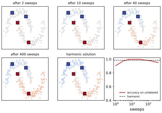
pp. 643 The manifold assumption says that similar points share labels. Label propagation (Zhu and Ghahramani, 2002) builds a graph on all \(M+N\) points with non-negative similarity weights \(w_{ij}\), known labels on the labeled nodes, and propagates them along the edges. With a transition matrix \[ T_{ij}=\frac{w_{ij}}{\sum_kw_{kj}} \tag{19.26} \] (the probability of propagating the label of node \(j\) to node \(i\)) and the \((M+N)\times C\) label matrix \(\bm Y\) (row \(i\) the class distribution of point \(i\)), repeat until \(\bm Y\) stops changing: (1) \(\bm Y\leftarrow\bm T\bm Y\); (2) renormalise the rows; (3) reset the labeled rows to their one-hot labels. The result is a labeling of the unlabeled points (a transductive method), which can then be used as training data for an inductive model. The method converges to a single fixed point involving the inverse of the unlabeled-to-unlabeled transition block. The weights decide everything; Euclidean similarity is adequate for simple data but not for high-dimensional complex data.
Filling the gap 19.10: label propagation has a harmonic solution; convergence; the printed algorithm p. 643, (19.26)
Proof
Result 19.2. Let \(\bm W\) be symmetric with non-negative entries, \(\bm D=\diag(\bm W\bm 1)\), \(\bm P=\bm D^{-1}\bm W\) (row-stochastic), and split nodes into labeled \(\ell\) and unlabeled \(u\). Suppose every connected component of the graph contains a labeled node. Then (i) \(\rho(\bm P_{uu})<1\); (ii) the clamped iteration \(\bm f_u\leftarrow\bm P_{uu}\bm f_u+\bm P_{u\ell}\bm f_\ell\) converges from any start to \(\bm f_u=(\bm I-\bm P_{uu})^{-1}\bm P_{u\ell}\bm f_\ell\); (iii) this is the unique minimiser over \(\bm f_u\) of the Dirichlet energy \(E(\bm f)=\frac12\sum_{ij}w_{ij}(f_i-f_j)^2=\bm f^\T(\bm D-\bm W)\bm f\) with \(\bm f_\ell\) clamped; (iv) \(0\le f_i\le1\) for \(\bm f_\ell\in\{0,1\}\), and for \(C\) classes the rows of the solution sum to one without any renormalisation.
Proof. (iii) \(\partial E/\partial\bm f_u=2[(\bm D-\bm W)\bm f]_u=2(\bm D_{uu}\bm f_u-\bm W_{uu}\bm f_u-\bm W_{u\ell}\bm f_\ell)\); setting it to zero and multiplying by \(\bm D_{uu}^{-1}\) gives \((\bm I-\bm P_{uu})\bm f_u=\bm P_{u\ell}\bm f_\ell\), i.e. \(f_i=\sum_jP_{ij}f_j\) at every unlabeled node: \(f\) is harmonic, a weighted average of its neighbours. (i) \(\bm P_{uu}\) is non-negative with row sums \(\le1\) (the missing mass goes to labeled neighbours). From any unlabeled node there is a path to a labeled node (component assumption), so \(\bm P_{uu}^k\) has row sums \(<1\) for \(k\ge\) the number of unlabeled nodes; hence \(\|\bm P_{uu}^k\|_\infty<1\) and \(\rho(\bm P_{uu})<1\). Then \(\bm I-\bm P_{uu}\) is invertible, \(E\) is strictly convex in \(\bm f_u\) (its Hessian \(2(\bm D-\bm W)_{uu}=2\bm D_{uu}(\bm I-\bm P_{uu})\) is positive definite), and the minimiser in (iii) is unique. (ii) The error \(\bm e_t=\bm f_u^{(t)}-\bm f_u^*\) obeys \(\bm e_{t+1}=\bm P_{uu}\bm e_t\), which tends to zero because \(\rho(\bm P_{uu})<1\) (the Neumann series \(\sum_k\bm P_{uu}^k\) converges). (iv) \(\bm f\) is the expected label at the labeled node at which a random walk started at \(i\) is absorbed (with transition probabilities \(P_{ij}\)): the absorption probabilities lie in \([0,1]\) and add to one over classes. Equivalently, by induction the iterates stay in \([0,1]\), and \((\bm I-\bm P_{uu})\bm 1_u=\bm P_{u\ell}\bm 1_\ell\) because \(\bm P\bm 1=\bm 1\), so the \(C\) columns of the solution add to \(\bm 1\). \(\square\)
The printed algorithm. With \(T_{ij}=w_{ij}/d_j\) (19.26) and \(\bm W\) symmetric, \(\bm T=\bm W\bm D^{-1}=\bm P^\T\): the update gives node \(i\) the average of its neighbours' labels weighted by \(1/d_j\), the degree of the sender, not by \(1/d_i\). The two coincide on a regular graph; in general the fixed point of the printed iteration (with row renormalisation and clamping) is not the harmonic solution, and the clamped linear part without renormalisation is not guaranteed to converge to it. On the two-moons example (300 points, two labels per class, Gaussian weights with \(\sigma=0.25\)) the printed algorithm settles after a few hundred sweeps, agrees with the harmonic labelling on 94.7 percent of the points, and its accuracy on the unlabeled points is 0.905 after 1 sweep, 0.996 after 10, 0.980 after 100 and 0.956 after 300, against 0.983 for the harmonic solution (Figure 19.S5): stopping early acts as a regulariser, as in gap 19.18. Computing the harmonic solution costs one linear solve with the \(u\times u\) matrix \(\bm I-\bm P_{uu}\), \(O(N^3)\) or, with sparse graphs and conjugate gradients, much less.
Inductive extension. The Nadaraya–Watson average \(f(\bm x)=\sum_jk(\bm x,\bm x_j)f_j/\sum_jk(\bm x,\bm x_j)\) with the same Gaussian kernel labels new points; the demo uses it for the test accuracy of label propagation. (Zhu et al., 2003, give the harmonic-function view; its energy and random-walk interpretations are proved above.) \(\square\)
See also: Elements of Statistical Learning, 14.3.7 (Gaussian mixtures), Bayesian and Probabilistic ML, 9.3 (the view of EM).
19.3.5 Consistency regularization
pp. 644–645 Consistency regularisation asks that a perturbation of the input (or of the model) not change the output much. This needs no labels, so it applies to unlabeled data. With \(\bm x'\sim q(\bm x'\given\bm x)\) (augmentation, noise, dropout) the combined loss over \(M\) labeled and \(N\) unlabeled points is \[ \mathcal L(\theta)=-\sum_{i=1}^M\log p_\theta(y=y_i\given\bm x_i)+\lambda\sum_{j=1}^N\big\|p_\theta(y\given\bm x_j)-p_\theta(y\given\bm x_j')\big\|^2 , \tag{19.27} \] the first term of the penalty usually treated as a constant (no gradient through it). Design choices: the weight \(\lambda\) (zero at the start, increased during training, so that the model does not reinforce its early mistakes); the perturbations \(q\) (label-preserving augmentations, strong ones working best); the distance (squared error, the Brier score, or KL divergence).
When no expert augmentation exists, virtual adversarial training (VAT, Miyato et al.) uses the perturbation that changes the output most, \(\bm\delta=\arg\max_{\bm\delta}\KL(p_\theta(y\given\bm x)\|p_\theta(y\given\bm x+\bm\delta))\), approximated by drawing \(\bm d\sim\N(\bm 0,\bm I)\) and setting \[ \bm\delta\leftarrow\nabla_{\bm\delta}\KL\big(p_\theta(y\given\bm x)\,\|\,p_\theta(y\given\bm x+\bm\delta)\big)\Big|_{\bm\delta=\xi\bm d},\qquad\bm x'=\bm x+\epsilon\frac{\bm\delta}{\|\bm\delta\|_2}, \tag{19.28, 19.29} \] with \(\xi\) small (for instance \(10^{-6}\)) and \(\epsilon\) setting the norm of the perturbation. Consistency regularisation also changes the geometry of training (the iterates travel further in weight space) and benefits from stochastic weight averaging (Athiwaratkun et al., 2019). Figure 19.11 compares the squared-error and KL penalties: squared error saturates, and its gradient vanishes, when the perturbed prediction is confidently wrong; KL grows without bound, has the scale of the cross entropy, and makes \(\lambda\) easier to tune.
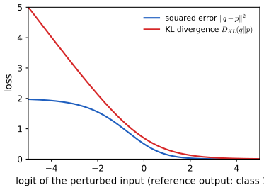
Filling the gap 19.11: gradients of the squared-error and KL consistency losses p. 645, Figure 19.11
Derivation
For a softmax output \(\bm p=\softmax(\bm a)\) the Jacobian is \(\bm J=\diag(\bm p)-\bm p\bm p^\T\) (symmetric, positive semi-definite). With a reference distribution \(\bm q\) held fixed, \[ \nabla_{\bm a}\|\bm q-\bm p\|^2=2\bm J(\bm p-\bm q),\qquad\nabla_{\bm a}\KL(\bm q\|\bm p)=\nabla_{\bm a}\Big(-\sum_cq_c\log p_c\Big)+\mathrm{const}=\bm p-\bm q , \] the second because \(\nabla_{\bm a}(-\log p_c)=\bm p-\bm e_c\). When the perturbed prediction becomes confident, \(\bm p\to\bm e_k\) for some class \(k\), \(\bm J\to\bm 0\) and the squared-error gradient vanishes whatever the disagreement with \(\bm q\): in the binary case with \(\bm q=(1,0)\) and \(p=\sigma(a)\) the loss is \(2(1-p)^2\) and the gradient with respect to \(a\) is \(-4p(1-p)^2\to0\) as \(a\to-\infty\) (at \(a=-9\) it is \(-5\times10^{-4}\)). The KL gradient \(\bm p-\bm q\) has norm up to \(\sqrt2\) and does not vanish; in the binary case it is \(\sigma(a)-1\to-1\). This is the advantage and the drawback the book describes: squared error leaves a model with very unstable predictions alone, and KL keeps pulling it back with a gradient of the scale of supervised cross entropy, which is why \(\lambda\) transfers between the two terms. \(\square\)
Filling the gap 19.12: the VAT recursion (19.28) is one step of power iteration on the Fisher information of the output p. 644, (19.28), (19.29)
Derivation
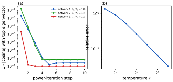
Let \(g(\bm\delta)=\KL(p(\cdot\given\bm x)\|p(\cdot\given\bm x+\bm\delta))=\sum_cp_c(\bm x)[\log p_c(\bm x)-\log p_c(\bm x+\bm\delta)]\). Then \(g(\bm 0)=0\), \(g\ge0\), so \(\bm 0\) is a minimum and \(\nabla g(\bm 0)=\bm 0\). The Hessian at \(\bm 0\) is \[ \bm H=\nabla^2g(\bm 0)=-\sum_cp_c\nabla^2\log p_c=\sum_cp_c\,\nabla\log p_c\,\nabla\log p_c^\T-\sum_c\nabla^2p_c=\sum_cp_c\,\nabla\log p_c\,\nabla\log p_c^\T , \] using \(\nabla^2\log p=\nabla^2p/p-\nabla\log p\nabla\log p^\T\) and \(\sum_c\nabla^2p_c=\nabla^2\sum_cp_c=\bm 0\); here all gradients are with respect to the input. \(\bm H\) is the Fisher information of the output distribution with respect to the input, symmetric and positive semi-definite. Hence \(g(\bm\delta)=\frac12\bm\delta^\T\bm H\bm\delta+O(\|\bm\delta\|^3)\), and the perturbation of norm \(\epsilon\) that changes the output most (to second order) maximises the Rayleigh quotient: it is \(\epsilon\bm v_1\) with \(\bm v_1\) the top eigenvector of \(\bm H\). Power iteration \(\bm d\leftarrow\bm H\bm d/\|\bm H\bm d\|\) converges to \(\bm v_1\) from any \(\bm d\) not orthogonal to it, the angle falling like \((\lambda_2/\lambda_1)^k\). Finally \(\nabla g(\xi\bm d)=\bm H\xi\bm d+O(\xi^2)\) (expand the gradient about the stationary point \(\bm 0\)), so (19.28) computes \(\bm H\bm d\) up to the factor \(\xi\) and an \(O(\xi^2)\) error by one backward pass, without ever forming the \(D\times D\) matrix \(\bm H\); (19.29) is the normalisation. Figure 19.S6a: for three random tanh networks with 4 outputs the iterate is aligned with the top eigenvector to \(1-|\cos|\approx10^{-8}\) after about 4 steps, the floor being the \(O(\xi)\) finite-difference error at \(\xi=10^{-4}\); the larger the gap between \(\lambda_1\) and \(\lambda_2\), the faster. In practice VAT uses one step, which suffices when the spectrum is dominated by one direction. \(\square\)
19.3.6 Deep generative models *
p. 646 A generative model of \(p(\bm x)\), fitted by minimising \(\mathcal L_U=-\sum_n\log p_\theta(\bm x_n)\), uses the unlabeled data directly; the question is how to turn \(p_\theta(\bm x)\) into a better supervised model.
19.3.6.1 Variational autoencoders
pp. 646–647 A VAE (Section 20.3.5; Foundations of Deep Learning, 19.2) has latent variables \(\bm z\sim p(\bm z)\), \(\bm x\sim p_\theta(\bm x\given\bm z)\), an encoder \(q_\lambda(\bm z\given\bm x)\) and is trained by the evidence lower bound. In the model M1 of Kingma et al. (2014) the latent code is a lower-dimensional, nonlinear, factorised representation that a classifier can use. In M2 there is also a class variable: \[ p_\theta(\bm x,y)=p_\theta(y)\,p_\theta(\bm x\given y)=p_\theta(y)\int p_\theta(\bm x\given y,\bm z)\,p_\theta(\bm z)\,\d\bm z, \tag{19.30} \] with \(p_\theta(\bm z)=\N(\bm 0,\bm I)\), \(p_\theta(y)=\operatorname{Cat}(\bm\pi_\theta)\) and a decoder \(p(\bm x\given f_\theta(y,\bm z))\); \(y\) is observed for labeled data, latent for unlabeled data. For labeled data, with \(q_\phi(\bm z\given y,\bm x)=\N(\bm\mu_\phi(y,\bm x),\diag\bm\sigma^2_\phi(\bm x))\), \[ \log p_\theta(\bm x,y)\ge\E_{q_\phi(\bm z\given\bm x,y)}\big[\log p_\theta(\bm x\given y,\bm z)+\log p_\theta(y)+\log p_\theta(\bm z)-\log q_\phi(\bm z\given\bm x,y)\big]=-\mathcal L(\bm x,y). \tag{19.31, 19.32} \] For unlabeled data the inference network is \(q_\phi(\bm z,y\given\bm x)=q_\phi(\bm z\given\bm x)q_\phi(y\given\bm x)\) (19.33)–(19.35) and \[ \log p_\theta(\bm x)\ge\E_{q_\phi(\bm z,y\given\bm x)}[\cdots]=-\sum_yq_\phi(y\given\bm x)\mathcal L(\bm x,y)+H(q_\phi(y\given\bm x))=-U(\bm x). \tag{19.36, 19.37} \] As \(q_\phi(y\given\bm x)\) then enters only the unlabeled bound, a classification loss on the labeled data is added: \[ \mathcal L(\theta)=\E_{(\bm x,y)\sim\mathcal D_\ell}[\mathcal L(\bm x,y)]+\E_{\bm x\sim\mathcal D_u}[U(\bm x)]+\alpha\,\E_{(\bm x,y)\sim\mathcal D_\ell}[-\log q_\phi(y\given\bm x)], \tag{19.38} \] \(\alpha\) trading generative against discriminative learning. The generative route lets one build in domain knowledge, for example a model of why labels are missing (people skip a health question when unwell).
19.3.6.2 Generative adversarial networks
pp. 647–648 A GAN has a generator mapping latent noise to data and a critic that tells generated from real data; it learns an implicit density, so the VAE route is unavailable. Semi-supervised GANs (Salimans et al., 2016; Odena, 2016) give the critic \(C+1\) outputs, the \(C\) classes plus "fake": it learns the class of labeled real data, "any class" (not fake) for unlabeled real data, and "fake" for generated data, while the generator tries to be classified as real (Figure 19.12, a diagram). With the standard cross-entropy GAN loss the critic minimises \[ -\E_{\bm x,y\sim p(\bm x,y)}\log p_\theta(y\given\bm x)-\E_{\bm x\sim p(\bm x)}\log[1-p_\theta(y=C+1\given\bm x)]-\E_{\bm z\sim p(\bm z)}\log p_\theta(y=C+1\given G(\bm z)) \tag{19.39} \] and the generator minimises \(\E_{\bm z}\log p_\theta(y=C+1\given G(\bm z))\) (19.40), a loss that saturates when the critic is confident; the practical non-saturating variant maximises \(\log(1-p_\theta(y=C+1\given G(\bm z)))\) instead.
19.3.6.3 Normalizing flows
pp. 648–649 A normalising flow is an invertible map \(f_\theta:\mathcal X\to\mathcal Z\) with density by change of variables \[ p(\bm x)=p(f(\bm x))\,\Big|\det\frac{\partial f}{\partial\bm x}\Big| . \tag{19.41} \] For labels \(y\in\{1,\dots,C\}\), choosing \(p(\bm z\given y=k)=\N(\bm z\given\bm\mu_k,\bm\Sigma_k)\) (Izmailov et al., 2020) makes the latent marginal a Gaussian mixture, with \[ p_X(\bm x\given y=k)=\N(f(\bm x)\given\bm\mu_k,\bm\Sigma_k)\Big|\det\frac{\partial f}{\partial\bm x}\Big| \tag{19.42} \] for labeled data and \(p(\bm x)=\sum_kp(\bm x\given y=k)p(y=k)\) for unlabeled data; maximising the joint likelihood \[ p(\mathcal D_\ell,\mathcal D_u\given\theta)=\prod_{(\bm x_i,y_i)\in\mathcal D_\ell}p(\bm x_i,y_i)\prod_{\bm x_j\in\mathcal D_u}p(\bm x_j) \tag{19.43} \] over the flow's parameters gives a Bayes classifier, \[ p_X(y=c\given\bm x)=\frac{p(\bm x\given y=c)p(y=c)}{p(\bm x)}=\frac{\N(f(\bm x)\given\bm\mu_c,\bm\Sigma_c)}{\sum_{k=1}^C\N(f(\bm x)\given\bm\mu_k,\bm\Sigma_k)}\ \ (p(y=c)=1/C), \tag{19.44} \] the Jacobian determinants cancelling in the ratio. See Foundations of Deep Learning, Chapter 18.
Filling the gap 19.13: the semi-supervised VAE bound (19.36)–(19.37), and what the flow model reduces to pp. 646–649
Derivation
Let \(q(\bm z,y\given\bm x)\) be any distribution over the latent variables. By Jensen's inequality (concavity of \(\log\)), \[ \log p(\bm x)=\log\sum_y\int p(\bm x,y,\bm z)\,\d\bm z\ \ge\ \E_{q(\bm z,y\given\bm x)}\big[\log p(\bm x\given y,\bm z)+\log p(y)+\log p(\bm z)-\log q(\bm z,y\given\bm x)\big], \] with equality iff \(q(\bm z,y\given\bm x)=p(\bm z,y\given\bm x)\) (the gap is \(\KL(q\|p(\cdot\given\bm x))\ge0\)). Factorise \(q(\bm z,y\given\bm x)=q(y\given\bm x)\,q(\bm z\given\bm x,y)\), so that \(\log q(\bm z,y\given\bm x)=\log q(y\given\bm x)+\log q(\bm z\given\bm x,y)\) and the bound becomes \[ \sum_yq(y\given\bm x)\,\E_{q(\bm z\given\bm x,y)}\big[\log p(\bm x\given y,\bm z)+\log p(y)+\log p(\bm z)-\log q(\bm z\given\bm x,y)\big]-\sum_yq(y\given\bm x)\log q(y\given\bm x), \] which is \(-\sum_yq(y\given\bm x)\mathcal L(\bm x,y)+H(q(y\given\bm x))=-U(\bm x)\) with \(\mathcal L(\bm x,y)\) exactly the labeled-data bound (19.32): the unlabeled bound is the labeled bound averaged over the inferred label plus the entropy of the label posterior. This requires \(q(\bm z\given\bm x,y)\), not the \(q(\bm z\given\bm x)\) printed in (19.33)–(19.34): with the factorisation \(q(\bm z\given\bm x)q(y\given\bm x)\) the inner term would contain \(\log q(\bm z\given\bm x)\) and an expectation over a \(y\)-independent \(q(\bm z\given\bm x)\), which is a different bound that does not equal (19.37) (the original M2 model of Kingma et al. uses \(q(\bm z\given y,\bm x)\)). All identities (the bound, equality at the exact posterior, and the decomposition (19.37)) were verified on a small discrete model with 4 latent states, 2 classes and 5 observations.
Flow classifier. If \(f\) is the identity, (19.42) is the Gaussian class-conditional density of quadratic discriminant analysis (Chapter 9), (19.44) its posterior with equal priors, and maximising (19.43) over \(\bm\mu_k,\bm\Sigma_k\) is exactly the semi-supervised EM of gap 19.7 (checked: with the sample means and covariances the posterior (19.44) equals scikit-learn's quadratic discriminant classifier to \(10^{-9}\)). The flow adds a learned invertible warp so that the classes become Gaussian in the latent space. \(\square\)
19.3.7 Combining self-supervised and semi-supervised learning
pp. 649–650 The two ideas combine (Chen et al., 2020): learn a representation on all the unlabeled data with SimCLR (Section 19.2.4.4), fine-tune it on the small labeled set (a teacher \(T\)), then use \(T\) to label the unlabeled data and distil (Hinton et al., 2014) the predictions into a student \(S\) by minimising \[ \mathcal L(T)=-\sum_{\bm x_i\in\mathcal D}\Big[\sum_yp_T(y\given\bm x_i;\tau)\log p_S(y\given\bm x_i;\tau)\Big], \tag{19.45} \] where \(\tau>0\) is a temperature applied to the softmax outputs (Figure 19.13, a diagram). If \(S\) has the form of \(T\) this is self-training (Section 19.3.1); normally the student is smaller, for example for a phone.
Filling the gap 19.14: the distillation gradient and its high-temperature limit p. 650, (19.45)
Derivation
Let \(\bm z_S,\bm z_T\) be the student and teacher logits, \(\bm q=\softmax(\bm z_S/\tau)\), \(\bm p=\softmax(\bm z_T/\tau)\). For one example, \(\mathcal L=-\sum_kp_k\log q_k=-\sum_kp_k(z_{S,k}/\tau)+\operatorname{lse}(\bm z_S/\tau)\) (using \(\sum_kp_k=1\)), so \[ \frac{\partial\mathcal L}{\partial z_{S,k}}=\frac1\tau\,(q_k-p_k). \] High temperature. For \(|z|/\tau\ll1\), \(\softmax(\bm z/\tau)_k=\frac{e^{z_k/\tau}}{\sum_je^{z_j/\tau}}=\frac1K\Big(1+\frac{z_k-\bar z}\tau+O(\tau^{-2})\Big)\) with \(\bar z=\frac1K\sum_jz_j\) (expand the numerator and the normaliser to first order). Hence \[ \frac{\partial\mathcal L}{\partial z_{S,k}}\approx\frac1{K\tau^2}\big[(z_{S,k}-\bar z_S)-(z_{T,k}-\bar z_T)\big], \] the gradient of the squared difference of the centred logits: at high temperature distillation is logit matching (Hinton et al., 2014, who note that matching logits is the limit, the temperature also needing a factor \(\tau^2\) to keep gradient magnitudes comparable). The relative error of this approximation falls like \(1/\tau\) (Figure 19.S6b: 0.36 at \(\tau=4\), 0.10 at 16, 0.025 at 64, 0.006 at 256). At \(\tau=1\) the gradient is the usual \(\bm q-\bm p\) of cross entropy with soft labels; a lower temperature emphasises the largest teacher probabilities. The gradient formula was confirmed against finite differences at \(\tau=1\) and 3. \(\square\)
19.4 Active learning
p. 650 In active learning the goal is to identify the mapping \(y=f(\bm x)\) with as few queried pairs \((\bm x,y)\) as possible. In query synthesis the algorithm may ask for the label of any input; in pool-based active learning it chooses among a large fixed pool of unlabeled points; in stream-based learning inputs arrive one by one and it decides whether to request each label. Related problems: Bayesian optimisation (find \(\bm x^*=\arg\min f\) in few queries, with a surrogate model) and experiment design (infer a parameter vector with carefully chosen \(\bm x\), "unsupervised active learning"). The section reviews the pool-based approach.
19.4.1 Decision-theoretic approach
p. 650 In the decision-theoretic approach (Kapoor et al., 2007; Roy and McCallum, 2001) the utility of querying \(\bm x\) is its value of information. The book writes \[ U(\bm x)\triangleq\E_{p(y\given\bm x,\mathcal D)}\Big[\min_a\big(\rho(a\given\mathcal D)-\rho(a\given\mathcal D,(\bm x,y))\big)\Big], \tag{19.46} \] with \(\rho(a\given\mathcal D)=\E_{p(\theta\given\mathcal D)}[\ell(\theta,a)]\) the posterior expected loss of action \(a\). Evaluating it for every candidate is expensive: for every possible answer \(y\) the posterior must be updated to see its effect on the future decision (a lookahead over belief states).
Filling the gap 19.15: the value of information is non-negative; the position of the minimum in (19.46) p. 650, (19.46)
Proof
Write \(\rho_y(a)=\rho(a\given\mathcal D,(\bm x,y))\) and \(\rho_0(a)=\rho(a\given\mathcal D)\). By Bayes' rule \(p(\theta\given\mathcal D,\bm x,y)\propto p(y\given\bm x,\theta)p(\theta\given\mathcal D)\) (the input \(\bm x\) is chosen, not generated by \(\theta\)), and \(p(y\given\bm x,\mathcal D)=\int p(y\given\bm x,\theta)p(\theta\given\mathcal D)\d\theta\), so by the tower property, for every fixed action, \[ \E_{p(y\given\bm x,\mathcal D)}\,\rho_y(a)=\rho_0(a). \] The value of information is the reduction of the Bayes risk achievable by seeing \(y\) before acting: \(\operatorname{VOI}(\bm x)=\min_a\rho_0(a)-\E_y\min_a\rho_y(a)\). It is non-negative: \(\E_y\min_a\rho_y(a)\le\min_a\E_y\rho_y(a)=\min_a\rho_0(a)\) (the expectation of a minimum is at most the minimum of the expectations), with equality iff the same action is optimal for every \(y\), when the observation could not change the decision.
The printed (19.46) has the minimum inside the expectation of a difference. By the same inequality, \(\E_y\min_a(\rho_0(a)-\rho_y(a))\le\min_a\E_y(\rho_0(a)-\rho_y(a))=\min_a0=0\): the printed quantity is never positive, so it cannot be the utility to maximise. The correct form puts the minimum separately on each term: \(U(\bm x)=\min_a\rho(a\given\mathcal D)-\E_{p(y\given\bm x,\mathcal D)}\min_a\rho(a\given\mathcal D,(\bm x,y))\ge0\), the expected improvement in the best achievable risk, which is the form in the cited papers. (Checked on random finite problems with 6 parameter values, 3 actions and 4 outcomes: the printed expression was \(\le0\) and the corrected one \(\ge0\) in all 200 trials.) \(\square\)
19.4.2 Information-theoretic approach
pp. 650–651 To avoid a task-specific loss one can aim to learn the model as well as possible. Lindley (1956) defines the utility of querying \(\bm x\) as the expected information gain about the parameters, the reduction in entropy, \[ U(\bm x)\triangleq H\big(p(\theta\given\mathcal D)\big)-\E_{p(y\given\bm x,\mathcal D)}\big[H\big(p(\theta\given\mathcal D,\bm x,y)\big)\big]. \tag{19.47} \] (The first term does not depend on \(\bm x\) but is kept for the next step.) Exercise 19.1 below shows that it equals the expected KL divergence between new and old posterior, \[ U'(\bm x)\triangleq\E_{p(y\given\bm x,\mathcal D)}\big[\KL\big(p(\theta\given\mathcal D,\bm x,y)\,\|\,p(\theta\given\mathcal D)\big)\big], \tag{19.48} \] and by the symmetry of mutual information \[ U(\bm x)=\MI(\theta;y\given\mathcal D,\bm x)=H\big(p(y\given\bm x,\mathcal D)\big)-\E_{p(\theta\given\mathcal D)}\big[H\big(p(y\given\bm x,\theta)\big)\big]. \tag{19.49–19.51} \] Only uncertainty about the output \(y\) is involved, not about the parameters. The first term of (19.51) prefers inputs whose predicted label is uncertain (using it alone is maximum entropy sampling, Sebastiani and Wynn, 1987), which fails on inherently ambiguous or mislabeled examples; the second term penalises inputs that are uncertain even when \(\theta\) is known. The rule therefore selects inputs where the model is confident for each \(\theta\) but the predictions disagree across \(\theta\): Bayesian active learning by disagreement (BALD, Houlsby et al., 2011), used for medical and astronomical images.
Filling the gap 19.16: (19.47)–(19.51), the closed form for linear-Gaussian models and an approximate closed form for BALD pp. 650–651
Derivation
(19.49)–(19.51). Conditionally on \((\mathcal D,\bm x)\), let \(\theta\sim p(\theta\given\mathcal D)\) and \(y\sim p(y\given\bm x,\theta)\), so the marginal of \(y\) is the predictive \(p(y\given\bm x,\mathcal D)\). Then \(\MI(\theta;y)=H(y)-H(y\given\theta)=H(p(y\given\bm x,\mathcal D))-\E_\theta H(p(y\given\bm x,\theta))\) is (19.51); and \(\MI(\theta;y)=H(\theta)-H(\theta\given y)\) with \(H(\theta\given y)=\E_yH(p(\theta\given\mathcal D,\bm x,y))\) is (19.47). Both equal the mean KL \(\E_y\KL(p(\theta\given y)\|p(\theta))\) (19.48): see the solution of Exercise 19.1.
Linear-Gaussian model. For \(y=\bm w^\T\bm x+\varepsilon\), \(\bm w\sim\N(\bm m,\bm\Sigma)\), \(\varepsilon\sim\N(0,s^2)\), the predictive is \(\N(\bm m^\T\bm x,s^2+\bm x^\T\bm\Sigma\bm x)\) and \(H(y\given\bm w)=\frac12\log(2\pi es^2)\) for every \(\bm w\), so (19.51) gives \(U(\bm x)=\frac12\log(1+\bm x^\T\bm\Sigma\bm x/s^2)\). Via (19.47): the posterior covariance after observing \(y\) is \(\bm\Sigma'=(\bm\Sigma^{-1}+\bm x\bm x^\T/s^2)^{-1}\), independent of \(y\), and \(\frac12\log\frac{\det\bm\Sigma}{\det\bm\Sigma'}=\frac12\log\det(\bm I+\bm\Sigma\bm x\bm x^\T/s^2)=\frac12\log(1+\bm x^\T\bm\Sigma\bm x/s^2)\) by the matrix determinant lemma: the same. (Confirmed numerically.) Here BALD is largest where the parameter uncertainty projected on \(\bm x\) is largest.
Maximum entropy fails on ambiguous inputs. If \(p(y=1\given\bm x,\theta)=\frac12\) for every \(\theta\) (a coin flip whatever the parameters), the predictive entropy is \(\log2\), the maximum possible, but \(\E_\theta H(p(y\given\bm x,\theta))=\log2\) too and \(U(\bm x)=0\): no label of that input is informative about \(\theta\).
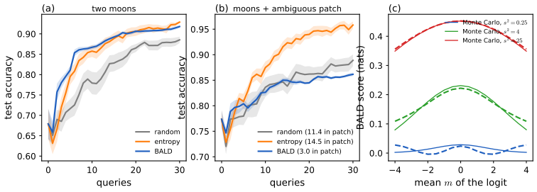
Binary logistic model, closed-form approximation. With posterior logit \(a=\bm w^\T\phi(\bm x)\sim\N(m,s^2)\) (Laplace approximation, Section 10.5.1) the first term of (19.51) is the entropy of the probit predictive \(\bar p=\sigma(m/\sqrt{1+\pi s^2/8})\) (Section 10.5.2). The second term \(\E_aH(\sigma(a))\) has no closed form, but \(H(\sigma(a))\) is a bump well approximated by \(\log2\,\exp(-a^2/(2b^2))\); the Gaussian integral \[ \E\big[\log2\,e^{-a^2/(2b^2)}\big]=\log2\,\frac{b}{\sqrt{s^2+b^2}}\exp\Big(-\frac{m^2}{2(s^2+b^2)}\Big) \] gives BALD \(\approx H(\bar p)-\log2\,\frac b{\sqrt{s^2+b^2}}e^{-m^2/(2(s^2+b^2))}\). Houlsby et al. (2011) derive this for a probit link with \(b^2=4\log2\) after the change of scale \(\sigma(a)\approx\Phi(\sqrt{\pi/8}\,a)\); fitting the width \(b\) by least squares over \(a\in[-12,12]\) gives \(b=1.852\) (against \(1.665\)), and the maximum error against Monte Carlo (\(10^5\) draws) over \(m\in[-4,4]\), \(s^2\in\{0.25,4,25\}\) is 0.030 nats, with the Houlsby value 0.058 (Figure 19.S7c). The tails of \(H(\sigma(a))\) decay like \(|a|e^{-|a|}\), slower than a Gaussian, so the approximation is best near \(m=0\); it is used only to rank candidates. When \(s^2\to0\) BALD tends to 0 even at \(m=0\) (a known coin flip): the score measures epistemic uncertainty only. \(\square\)
See also: Section 10.5 (Laplace approximation and the probit predictive); Section 6.3 (mutual information).
19.4.3 Batch active learning
p. 651 A greedy, myopic strategy picks one point at a time as if it were the last. With a budget of \(B\) labels the criterion becomes the information gain of the batch, \(U(\bm x_{1:B})=H(p(\theta\given\mathcal D))-\E_{p(\bm y\given\bm x_{1:B},\mathcal D)}[H(p(\theta\given\bm y,\bm x_{1:B},\mathcal D))]\), whose maximisation is NP-hard in \(B\) (Krause and Guestrin, 2005; Kolb et al., 1995). Under a condition the greedy strategy is nevertheless near-optimal: \(f(S)=H(p(\theta\given\mathcal D))-H(p(\theta\given\bm y_S,\mathcal D))\), as a function of the set \(S\) of queried inputs, satisfies \(f(\emptyset)=0\), is non-decreasing (more information never hurts) and is submodular (Krause and Guestrin, 2005), so greedy selection is within a constant factor of optimal; with BALD as the criterion this is BatchBALD (Kirsch et al., 2019).
Filling the gap 19.17: the information gain is monotone and submodular, and greedy is within \(1-1/e\) p. 651
Proof
Let the observations \(y_1,\dots,y_n\) at candidate inputs \(\bm x_1,\dots,\bm x_n\) be conditionally independent given \(\theta\) (the standard model). For a subset \(S\) let \(F(S)=\MI(\theta;\bm y_S)\) (conditioning on \(\mathcal D\) throughout).
(a) Monotone. Chain rule: \(F(S\cup\{j\})-F(S)=\MI(\theta;y_j\given\bm y_S)\ge0\).
(b) Submodular (diminishing returns): for \(S\subseteq T\) and \(j\notin T\), \(F(S\cup\{j\})-F(S)\ge F(T\cup\{j\})-F(T)\). Write the marginal gain as \(\MI(\theta;y_j\given\bm y_S)=H(y_j\given\bm y_S)-H(y_j\given\theta,\bm y_S)\). Conditional independence gives \(H(y_j\given\theta,\bm y_S)=H(y_j\given\theta)\) for every \(S\), a constant. And \(H(y_j\given\bm y_S)\ge H(y_j\given\bm y_T)\) because conditioning on more variables cannot increase entropy. So the gain from \(j\) given \(S\) is at least the gain given \(T\).
(c) Greedy guarantee (Nemhauser, Wolsey and Fisher, 1978). Let \(F\) be monotone submodular with \(F(\emptyset)=0\), \(S^*\) an optimal set of size \(B\), and \(G_i\) the greedy set after \(i\) steps, each step adding the element of largest marginal gain \(\Delta(j\given G_i)=F(G_i\cup\{j\})-F(G_i)\). Then \[ F(S^*)\le F(G_i\cup S^*)\le F(G_i)+\sum_{j\in S^*}\Delta(j\given G_i)\le F(G_i)+B\,[F(G_{i+1})-F(G_i)], \] using monotonicity, then submodularity (the gain of the whole set \(S^*\) is at most the sum of the gains of its elements), then the greedy choice (every gain is \(\le\) the gain of the chosen element). Rearranged, with \(\delta_i=F(S^*)-F(G_i)\): \(\delta_{i+1}\le(1-\frac1B)\delta_i\), so \(\delta_B\le(1-\frac1B)^BF(S^*)\le e^{-1}F(S^*)\), i.e. \(F(G_B)\ge(1-1/e)F(S^*)\approx0.63\,F(S^*)\). \(\square\)
Numerical experiment. For \(F(S)=\frac12\log\det(\bm I+\bm X_S\bm\Sigma\bm X_S^\T/s^2)\) (the information gain of a linear-Gaussian model, whose entries are conditionally independent given \(\bm w\)) on 6 random instances with 12 candidates, monotonicity and diminishing returns held in all 180 random tests, and greedy selection of \(B=3\) reached at least 0.962 of the exhaustive optimum (the guarantee is 0.632). The book's notation \(f(Y)\) for a function of the set of queried inputs is loose: it is a set function of the inputs, with the responses averaged over.
19.5 Meta-learning
pp. 651–652 A learning algorithm is a function \(A\) from data to parameters, \(\theta=A(\mathcal D;\phi)\), with its own parameters \(\phi\) (the initial value of \(\theta\), a learning rate, ...). Meta-learning (learning to learn, Thrun and Pratt, 1997) learns \(\phi=M(\mathcal D_{1:J})\) from a collection of datasets, then applies \(A(\cdot;\phi)\) to a new dataset \(\mathcal D_{J+1}\) (Figure 19.14, a graphical model).
19.5.1 Model-agnostic meta-learning (MAML)
p. 652 A natural model is hierarchical Bayesian: task parameters \(\theta_j\sim p(\theta_j\given\xi)\) share a prior that pools statistical strength among data-poor tasks, and meta-learning is learning the prior. An efficient approximation is empirical Bayes (Section 4.6.5.3) with a cross-validation approximation to the marginal likelihood (Section 5.2.4): \[ \xi^*=\arg\max_\xi\ \frac1J\sum_{j=1}^J\log p\big(\mathcal D_{\rm valid}^j\given\hat\theta_j(\xi,\mathcal D_{\rm train}^j)\big), \tag{19.52} \] with \(\hat\theta_j\) a point estimate from task \(j\)'s training set and the prior \(\xi\). In model-agnostic meta-learning (MAML, Finn et al., 2017) the point estimate is \(K\) steps of gradient ascent from \(\xi\) with learning rate \(\eta\); this is equivalent to an approximate MAP estimate with a Gaussian prior centred at \(\xi\), whose strength is controlled by the number of steps (Santos, 1996; Grant et al., 2018): fast adaptation of task-specific weights from the shared prior \(\xi\).
Filling the gap 19.18: \(K\) gradient steps from \(\xi\) are a MAP estimate with a Gaussian prior centred at \(\xi\) p. 652
Proof
Result 19.3. Let \(\mathcal L(\theta)=\frac12(\theta-\hat\theta)^\T\bm H(\theta-\hat\theta)\) with \(\bm H\) symmetric positive definite and eigenvalues \(h_i\), minimised by \(\hat\theta\) (the unregularised estimate, e.g. a least-squares or Gaussian-likelihood fit). Gradient descent from \(\theta_0=\xi\) with step \(\eta\), \(0<\eta h_i<1\), gives after \(K\) steps \(\theta_K=\hat\theta+(\bm I-\eta\bm H)^K(\xi-\hat\theta)\). The MAP estimate with prior \(\N(\xi,\bm\Lambda^{-1})\), \(\bm\Lambda=\bm H[(\bm I-\eta\bm H)^{-K}-\bm I]^{-1}\), is the same point.
Proof. (i) GD. \(\theta_{t+1}-\hat\theta=(\bm I-\eta\bm H)(\theta_t-\hat\theta)\); iterate. (ii) MAP. Minimising \(\mathcal L(\theta)+\frac12(\theta-\xi)^\T\bm\Lambda(\theta-\xi)\) gives \(\bm H(\theta-\hat\theta)+\bm\Lambda(\theta-\xi)=\bm 0\), i.e. \(\theta-\hat\theta=(\bm H+\bm\Lambda)^{-1}\bm\Lambda(\xi-\hat\theta)\). (iii) Match. Both are functions of \(\bm H\) and commute. We need \((\bm H+\bm\Lambda)^{-1}\bm\Lambda=(\bm I-\eta\bm H)^K\), i.e. \(\bm I+\bm H\bm\Lambda^{-1}=(\bm I-\eta\bm H)^{-K}\), so \(\bm\Lambda=\bm H[(\bm I-\eta\bm H)^{-K}-\bm I]^{-1}\), positive definite when \(0<\eta h_i<1\) (so that \((1-\eta h_i)^{-K}>1\)). \(\square\)
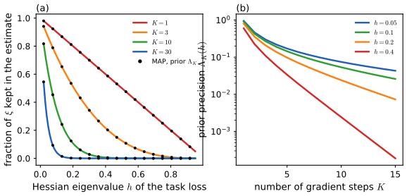
Reading the result. Along the eigendirection with curvature \(h\) the prior precision is \(\Lambda_K(h)=h/[(1-\eta h)^{-K}-1]\): for small \(K\eta h\) it is \(\approx1/(K\eta)\), isotropic and decreasing in \(K\) (a prior as strong as \(1/(K\eta)\)); at \(K=1\) it is exactly \((1-\eta h)/\eta\); as \(K\to\infty\) it tends to 0 (no prior: the maximum-likelihood fit). So "the strength is controlled by the number of steps" is correct, with the refinement that the prior is anisotropic: high-curvature directions are released faster. For \(\eta h\ge1\) the factor \((1-\eta h)^K\) alternates in sign for odd \(K\) and no positive precision reproduces it. For a non-quadratic loss the statement holds locally, to first order in the departure from quadratic, with \(\bm H\) the Hessian at the start (the "approximate" of the book). Figure 19.S9 shows the fraction \((1-\eta h)^K\) of \(\xi\) retained against the curvature for four \(K\), with the MAP values at \(\Lambda_K(h)\) on top (agreement to \(10^{-16}\) in the numerical experiment), and \(\Lambda_K(h)\) against \(K\). The same argument explains why a small learning rate and few steps (fine-tuning, gap 19.3) or early stopping (Foundations of Deep Learning, 9.3.1) regularise towards the starting point. \(\square\)
Filling the gap 19.19: the MAML meta-gradient and its first-order approximation p. 652, Section 19.5.1
Derivation
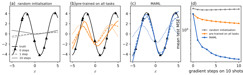
Take one inner step, \(\theta'(\xi)=\xi-\eta\nabla\mathcal L_{\rm train}(\xi)\), and meta-objective \(\mathcal M(\xi)=\mathcal L_{\rm valid}(\theta'(\xi))\). The chain rule with \(\partial\theta'/\partial\xi=\bm I-\eta\bm H_{\rm train}(\xi)\) (the Jacobian of the update map, \(\bm H_{\rm train}\) the training Hessian, symmetric) gives \[ \nabla_\xi\mathcal M=\big(\bm I-\eta\bm H_{\rm train}(\xi)\big)\,\nabla\mathcal L_{\rm valid}(\theta'). \] For \(K\) steps the Jacobian is the product \(\prod_{k=0}^{K-1}(\bm I-\eta\bm H_{\rm train}(\theta_k))\). The Hessian term makes MAML a second-order method: it is computed with Hessian-vector products by differentiating through the inner loop. First-order MAML drops it, \(\nabla_\xi\mathcal M\approx\nabla\mathcal L_{\rm valid}(\theta')\): exact when \(\eta\bm H\) is small. The first-order update is the gradient at the adapted point applied to the initialisation. In the experiment of Figure 19.S8 the full second-order gradient (through the inner step with automatic differentiation) agreed with a finite-difference estimate of the directional derivative to 8 digits (\(-3.92499621\) both). The relation with (19.52): the meta-objective is the validation log-likelihood of the adapted parameters, a cross-validation (hold-out) estimate of the marginal likelihood, which by the chain rule \(p(\mathcal D)=\prod_ip(y_i\given y_{<i})\) averages the predictive of later data given earlier data. \(\square\)
19.6 Few-shot learning
p. 653 People learn from very few examples. Few-shot learning is the machine version; with one example per class it is one-shot, with none zero-shot (as CLIP, Section 19.2.4.5). It is evaluated as \(C\)-way \(N\)-shot classification: learn to separate \(C\) classes from \(N\) training examples of each (Figure 19.15, a diagram, shows \(C=3\), \(N=2\)). Training examples are too few to learn from scratch, so meta-learning is used: the meta-algorithm \(M\) is trained on tasks \(j=1,\dots,J\), each with a labeled support set from which it returns a predictor \(f^j\) that is scored on a disjoint query set of the same task; the classes of the training tasks and of the test task do not overlap, so \(M\) must learn to classify images in general rather than any particular labels.
19.6.1 Matching networks
pp. 653–654 One approach learns a distance \(d_\theta(\bm x,\bm x')\) on a large other data set and uses it in a nearest-neighbour classifier: a semi-parametric model \(p_\theta(y\given\bm x,S)\) with the support set \(S\) as data (widely used for fine-grained recognition, for faces and product images). A matching network (Vinyals et al., 2016) generalises this with an adaptive similarity kernel \(a_\theta(\bm x,\bm x_n;S)\ge0\), \[ p_\theta(y\given\bm x,S)=\ind\Big(y=\sum_{n\in S}a_\theta(\bm x,\bm x_n;S)\,y_n\Big)\ \text{(as printed)},\qquad a(\bm x,\bm x_n;S)=\frac{\exp(c(f(\bm x),g(\bm x_n)))}{\sum_{n'=1}^N\exp(c(f(\bm x),g(\bm x_{n'})))}, \tag{19.53, 19.54} \] where \(c\) is cosine similarity and \(f,g\) embeddings (possibly equal); an attention kernel compares \(\bm x\) with \(\bm x_n\) in the context of all labeled examples (Section 15.4). Training uses episodes: with \(\mathcal D\) a large labeled set and \(p(L)\) a distribution over label subsets, sample a few labels \(L\sim p(L)\), a support set \(S\sim L\) and a query set \(T\sim L\), and maximise \[ \mathcal L(\theta;\mathcal D)=\E_{L\sim p(L)}\Big[\E_{S\sim L,T\sim L}\Big[\sum_{(\bm x,y)\in T}\log p_\theta(y\given\bm x,S)\Big]\Big]. \tag{19.55} \] After training \(\theta\) is frozen and (19.53) is applied to a new support set.
Filling the gap 19.20: the matching-network classifier is a kernel (Nadaraya–Watson) classifier, and what (19.53) should say pp. 653–654, (19.53), (19.54)
Derivation
What (19.53) means. As printed, \(\ind(y=\sum_na_ny_n)\) is not a probability distribution over labels: with one-hot \(y_n\) the weighted sum is a vector in the simplex, not a label. The intended model is the attention-weighted vote \[ p_\theta(y=k\given\bm x,S)=\sum_{n\in S}a_\theta(\bm x,\bm x_n;S)\,\ind(y_n=k),\qquad\sum_kp_\theta(y=k\given\bm x,S)=\sum_na_n=1, \] a probability distribution because the attention weights (19.54) are a softmax. Also \(c\) in (19.54) must be a cosine similarity (larger when the points are close); a distance would reverse the ordering.
Kernel classifier. Define \(\kappa(\bm x,\bm x_n)=\exp(c(f(\bm x),g(\bm x_n)))\). Then \(p(y=k\given\bm x,S)=\sum_n\kappa(\bm x,\bm x_n)\ind(y_n=k)/\sum_n\kappa(\bm x,\bm x_n)\): the Nadaraya–Watson classifier of Section 16.3.5 (see also the Bishop course, 6.3.1) in embedding space. With a temperature \(\tau\), \(\kappa=\exp(c/\tau)\): as \(\tau\to0\) all the mass goes to the support point with the largest cosine similarity, i.e. the 1-nearest-neighbour rule in the embedding; as \(\tau\to\infty\) every point gets weight \(1/|S|\) and the prediction is the class frequencies of the support set. (All three facts, the distribution property, the \(\tau\to0\) limit and the Nadaraya–Watson equality, were confirmed numerically.) The episodic objective (19.55) matches training to evaluation: each episode has the same structure, \(C\) classes with \(N\) shots, that a test task will have, so the embedding is optimised for exactly the task of classifying from a small support set. \(\square\)
19.7 Weakly supervised learning
p. 655 In weakly supervised learning not every feature vector has an exact label. Three scenarios are treated. (i) Each case has a distribution over labels \(p(y\given\bm x_n)\): train by minimising the cross entropy \[ \mathcal L(\theta)=-\sum_n\sum_yp(y\given\bm x_n)\log q_\theta(y\given\bm x_n), \tag{19.56} \] which is maximum likelihood with soft labels. Replacing exact labels by a soft version with, say, 90 percent of the mass on the observed label and the rest spread uniformly over the others is label smoothing (Müller et al., 2019), a form of regularisation. (ii) Multi-instance learning (Dietterich et al., 1997): a bag \(\bm x_n=\{\bm x_{n,1},\dots,\bm x_{n,B}\}\) has a label \(y_n=\bigvee_by_{nb}\) (positive if any member is, negative if all are) while the instances \(y_{nb}\) are unobserved; examples include COVID-19 exposure risk scores. (iii) Distant supervision (Mintz et al., 2009): a database fact such as Married(B,M) labels every sentence that mentions both entities as a positive example of the relation, which also labels false positives; the noisy labels can be handled as in Section 10.4.
Filling the gap 19.21: soft labels, the label-smoothing optimum and the noisy-OR bag model p. 655, (19.56)
Derivation
Soft labels. \(\mathcal L(\theta)=\sum_n\big[H(p_n)+\KL(p_n\|q_\theta(\cdot\given\bm x_n))\big]\), where \(p_n=p(\cdot\given\bm x_n)\). The entropy does not depend on \(\theta\), so (19.56) minimises the KL divergence from the label distributions to the model, and by Gibbs' inequality the global minimiser is \(q_\theta=p_n\) for every \(n\) whenever the model class contains it. (If the soft label is the posterior \(p(y\given\bm x_n,\text{partial information})\) of a latent label this is one step of EM, as in gap 19.7.)
Label smoothing. With true class \(k\) and a smoothing level \(\alpha\), the target puts \(1-\alpha\) on \(k\) and \(\alpha/(K-1)\) on each other class. If the model can realise any logits the optimum is \(\bm q=\)target, so the logit gap between the true class and another is \(\log\frac{(1-\alpha)(K-1)}\alpha\), finite: for \(K=5\), \(\alpha=0.1\) the gap is 3.58 (numerical optimisation: 3.58352), and the cross-entropy minimiser no longer drives the logits to infinity on separable data, in contrast to the hard-label case of Result 10.1. (A common variant spreads \(\alpha\) uniformly over all \(K\) classes including the true one.)
Multi-instance learning with the noisy-OR. Suppose instance labels are conditionally independent given the instances, \(p(y_{nb}=1\given\bm x_{nb})=p_{nb}=\sigma(\bm w^\T\bm x_{nb})\). The bag is positive iff some instance is, so \[ P(y_n=0)=\prod_b(1-p_{nb}),\qquad P(y_n=1)=1-\prod_b(1-p_{nb}). \] For a negative bag, \(-\log P=-\sum_b\log(1-p_{nb})\) with gradient \(\sum_bp_{nb}\bm x_{nb}\). For a positive bag put \(Q=\prod_b(1-p_{nb})\); since \(\partial Q/\partial\bm w=-Q\sum_bp_{nb}\bm x_{nb}\) (because \(\partial\log(1-p)/\partial\bm w=-p\,\bm x\)), \[ \nabla_{\bm w}\big(-\log(1-Q)\big)=-\frac{Q}{1-Q}\sum_bp_{nb}\bm x_{nb}. \] (Both gradients agree with finite differences to \(10^{-8}\).) Positive bags thus pull the weights in the direction of their most positive instances, scaled by the posterior-like factor \(Q/(1-Q)\), which is small once some instance is already confidently positive. Figure 19.S10: bags of 5 points in the plane, negative instances \(\N(\bm 0,\bm I)\), positive instances shifted by \((1.77,1.77)\), each instance of a positive bag positive with probability 0.3 (at least one forced); with 150 training bags the instance-level accuracy on 300 test bags is 0.923 for the noisy-OR fit, against 0.525 when every instance is simply labeled with its bag and 0.825 for always predicting "negative". \(\square\)
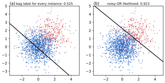
19.8 Exercises
The one exercise of Chapter 19 (Murphy, 2022, p. 656), restated in my own words, with a complete solution (hidden).
Exercise 19.1 (information gain equations). For the utility of querying an input \(\bm x\) in active learning, consider \[ U(\bm x)\triangleq H\big(p(\theta\given\mathcal D)\big)-\E_{p(y\given\bm x,\mathcal D)}\big[H\big(p(\theta\given\mathcal D,\bm x,y)\big)\big], \tag{19.57} \] \[ U'(\bm x)\triangleq\E_{p(y\given\bm x,\mathcal D)}\big[\KL\big(p(\theta\given\mathcal D,\bm x,y)\,\|\,p(\theta\given\mathcal D)\big)\big]. \tag{19.58} \] Prove that they are equal.
Solution
Setting. The query input \(\bm x\) is chosen by us, so \(\theta\) is independent of the choice: the joint law of \((\theta,y)\) given \((\mathcal D,\bm x)\) is \(p(\theta\given\mathcal D)\,p(y\given\bm x,\theta)\). Its \(y\)-marginal is the predictive \(p(y\given\bm x,\mathcal D)=\int p(y\given\bm x,\theta)p(\theta\given\mathcal D)\d\theta\) and, by Bayes' rule, the conditional of \(\theta\) given \(y\) is \(p(\theta\given\mathcal D,\bm x,y)\). Hence, for any function \(g(\theta)\) (integrable), \[ \E_{p(y\given\bm x,\mathcal D)}\E_{p(\theta\given\mathcal D,\bm x,y)}\,g(\theta)=\E_{p(\theta\given\mathcal D)}\,g(\theta) \tag{\(\ast\)} \] (the tower property: averaging the posterior over the predictive distribution of \(y\) returns the prior).
Proof. Write the KL divergence out: \[ U'(\bm x)=\E_y\E_{\theta\given y}\big[\log p(\theta\given\mathcal D,\bm x,y)-\log p(\theta\given\mathcal D)\big]=-\E_yH\big(p(\theta\given\mathcal D,\bm x,y)\big)-\E_y\E_{\theta\given y}\log p(\theta\given\mathcal D). \] The first term is the (negative of the) expected posterior entropy. In the second, \(\log p(\theta\given\mathcal D)\) does not depend on \(y\), so by \((\ast)\) with \(g(\theta)=\log p(\theta\given\mathcal D)\), \(\E_y\E_{\theta\given y}\log p(\theta\given\mathcal D)=\E_{p(\theta\given\mathcal D)}\log p(\theta\given\mathcal D)=-H(p(\theta\given\mathcal D))\). Therefore \[ U'(\bm x)=-\E_yH\big(p(\theta\given\mathcal D,\bm x,y)\big)+H\big(p(\theta\given\mathcal D)\big)=U(\bm x).\ \square \]
Computation. For a Bernoulli parameter \(\theta\) with prior \(\operatorname{Beta}(2,3)\) and one binary observation, on a grid of 20001 points: \(H(p(\theta))-\E_yH(p(\theta\given y))=0.08967832\) nats, \(\E_y\KL(p(\theta\given y)\|p(\theta))=0.08967832\), and \(H(y)-\E_\theta H(y\given\theta)=0.08967832\), the same number three ways, confirming (19.57)=(19.58)=(19.51). The posterior entropies are differential entropies; the equality does not depend on that choice since only differences appear.
Demonstrations
| Page | What it shows | In the notes |
|---|---|---|
| Semi-supervised learning from a few labels | Two moons (RBF logistic model) or two blobs (linear model) with up to ten labeled points per class and 300 unlabeled: supervised fit, self-training with a threshold, entropy minimisation with a weight, label propagation with a graph width; accuracy on test and unlabeled points against the supervised fit. Presets: 1 supervised only; 2 self-training; 3 label propagation; 4 a graph that is too wide; 5 self-training reinforces a mistake; 6 entropy minimisation repairs it. | 19.3.1, 19.3.2, 19.3.4, gap 19.8, gap 19.10 |
| Active learning with BALD | A pool of 300 points and a Laplace logistic model refitted after each query; random, maximum-entropy and BALD rules from the same start, with the predictive probability, the score of each point, the next query and the learning curves; a second pool with a coin-flip patch. Presets: 1 BALD; 2 maximum entropy; 3 the patch under maximum entropy; 4 the patch under BALD; 5 random queries. | 19.4.2, gap 19.16, gap 19.17 |
| Few-shot regression with MAML | Sinusoid regression by a small network from a random, a pre-trained and a meta-learned initialisation, adapted by plain gradient steps on up to ten points; fits and test error against the number of steps. Presets: 1 one step on ten points; 2 ten steps; 3 five points; 4 a tiny amplitude; 5 before adaptation. | 19.5.1, gap 19.18, gap 19.19 |
The Python code that produces every figure of this page is code/ch19_learning_with_fewer_labels.py (see the code index). Companion demos: EM for mixtures, Bayesian regression, early stopping.
Notes on the book
Points where the book is imprecise or wrong
- (19.46), the position of the minimum. The printed utility puts the minimum over actions around the difference \(\rho(a\given\mathcal D)-\rho(a\given\mathcal D,(\bm x,y))\) inside the expectation. Since \(\E_y\rho(a\given\mathcal D,(\bm x,y))=\rho(a\given\mathcal D)\) for each \(a\), the printed quantity is never positive. The value of information is \(\min_a\rho(a\given\mathcal D)-\E_y\min_a\rho(a\given\mathcal D,(\bm x,y))\ge0\) (gap 19.15).
- Section 19.3.2, sharpening at \(T=1\). "At \(T=1\) this is equivalent to entropy minimization" holds for the value of the loss only. With the target held fixed, as it is in practice, the gradient at \(T=1\) is zero; the entropy has a non-zero gradient (gap 19.7).
- (19.33)–(19.34) against (19.37). The inference network for unlabeled data must be \(q_\phi(\bm z\given\bm x,y)q_\phi(y\given\bm x)\) for (19.36)–(19.37) to follow; with the printed \(q_\phi(\bm z\given\bm x)q_\phi(y\given\bm x)\) the bound is a different one (gap 19.13).
- (19.53), (19.54). The indicator of a weighted sum of one-hot labels is not a probability; the matching-network prediction is \(\sum_na_n\ind(y=y_n)\). In (19.54) \(c\) must be a cosine similarity, not a distance (gap 19.20).
- Section 19.3.4, the transition matrix and the fixed point. The column-normalised \(\bm T\) of (19.26) weights a neighbour's label by the inverse degree of the sender; the harmonic solution of Zhu et al. (2003), whose closed form involves \((\bm I-\bm P_{uu})^{-1}\), uses the row-normalised \(\bm P=\bm D^{-1}\bm W\). The printed algorithm (with row renormalisation) has a different fixed point, which agrees with the harmonic labelling on most but not all points (gap 19.10).
- (19.12). The loss is described as averaged over minibatches but printed as a sum; it needs a factor \(1/N\) (a constant that only rescales the learning rate).
- (19.15), which parameters are maximised. As printed, the maximisation over \(\theta\) acts on both terms, so the features would also maximise the task loss; the intended saddle point has the feature extractor minimise the task loss and maximise the domain-classifier loss while the domain classifier (parameters absent from the formula) minimises its own loss, as in Ganin et al. (2016).
- Section 19.2.2, "low-rank". The adapter matrix \(\bm\alpha\in\R^{C\times D}\) is unconstrained, so the perturbation of the filter is low-rank only if \(\bm\alpha\) is made low-rank; it acts on a single mode of the filter tensor (parallel adapters, on the centre tap only) (gap 19.4).
- Section 19.5.1, "equivalent to MAP". The equivalence is exact for a quadratic loss with step \(0<\eta h<1\); the prior is anisotropic (precision \(h/[(1-\eta h)^{-K}-1]\) along a direction of curvature \(h\)), not a single scalar strength (gap 19.18).
- Section 19.1.1. Both the search over augmentations by reinforcement learning or Bayesian optimisation and the learning of combinations of augmentations are called "AutoAugment" in consecutive sentences; Cubuk et al. (2019) is the reinforcement-learning policy search, Lim et al. (2019) a faster Bayesian-optimisation variant.
- Section 19.4.3, the set function. The information gain \(f\) is written as a function of the responses \(Y\); it is a set function of the queried inputs (with the responses averaged out), monotone and submodular when the observations are conditionally independent given \(\theta\) (gap 19.17).
- (19.40). The generator loss \(\E\log p_\theta(y=C+1\given G(\bm z))\) saturates when the critic recognises fakes; the practical (non-saturating) generator maximises \(\log(1-p_\theta(y=C+1\given G(\bm z)))\) (Goodfellow et al., 2014).
References
- Murphy, K. P. (2022). Probabilistic Machine Learning: An Introduction. MIT Press, Cambridge, MA. Chapter 19, pp. 627–656. probml.github.io/pml-book/book1.html.
- Athiwaratkun, B., Finzi, M., Izmailov, P. and Wilson, A. G. (2019). There are many consistent explanations of unlabeled data: why you should average. International Conference on Learning Representations.
- Bishop, C. M. (1995). Training with noise is equivalent to Tikhonov regularization. Neural Computation, 7(1), 108–116.
- Blum, A. and Mitchell, T. (1998). Combining labeled and unlabeled data with co-training. Conference on Computational Learning Theory.
- Bridle, J. S., Heading, A. J. R. and MacKay, D. J. C. (1992). Unsupervised classifiers, mutual information and "phantom targets". Advances in Neural Information Processing Systems, 4.
- Chapelle, O., Weston, J., Bottou, L. and Vapnik, V. (2001). Vicinal risk minimization. Advances in Neural Information Processing Systems, 13.
- Chen, T., Kornblith, S., Norouzi, M. and Hinton, G. (2020). A simple framework for contrastive learning of visual representations. International Conference on Machine Learning.
- Chen, T., Kornblith, S., Swersky, K., Norouzi, M. and Hinton, G. (2020). Big self-supervised models are strong semi-supervised learners. Advances in Neural Information Processing Systems, 33.
- Cubuk, E. D., Zoph, B., Mane, D., Vasudevan, V. and Le, Q. V. (2019). AutoAugment: learning augmentation strategies from data. Conference on Computer Vision and Pattern Recognition.
- Dietterich, T. G., Lathrop, R. H. and Lozano-Pérez, T. (1997). Solving the multiple instance problem with axis-parallel rectangles. Artificial Intelligence, 89(1–2), 31–71.
- Finn, C., Abbeel, P. and Levine, S. (2017). Model-agnostic meta-learning for fast adaptation of deep networks. International Conference on Machine Learning.
- Ganin, Y., Ustinova, E., Ajakan, H., et al. (2016). Domain-adversarial training of neural networks. Journal of Machine Learning Research, 17(59), 1–35.
- Goodfellow, I., Pouget-Abadie, J., Mirza, M., et al. (2014). Generative adversarial nets. Advances in Neural Information Processing Systems, 27.
- Grandvalet, Y. and Bengio, Y. (2005). Semi-supervised learning by entropy minimization. Advances in Neural Information Processing Systems, 17.
- He, K., Fan, H., Wu, Y., Xie, S. and Girshick, R. (2020). Momentum contrast for unsupervised visual representation learning. Conference on Computer Vision and Pattern Recognition.
- Hinton, G., Vinyals, O. and Dean, J. (2015). Distilling the knowledge in a neural network. arXiv:1503.02531 (the book cites a 2014 workshop version).
- Houlsby, N., Huszár, F., Ghahramani, Z. and Lengyel, M. (2011). Bayesian active learning for classification and preference learning. arXiv:1112.5745.
- Houlsby, N., Giurgiu, A., Jastrzebski, S., et al. (2019). Parameter-efficient transfer learning for NLP. International Conference on Machine Learning.
- Izmailov, P., Kirichenko, P., Finzi, M. and Wilson, A. G. (2020). Semi-supervised learning with normalizing flows. International Conference on Machine Learning.
- Kingma, D. P., Rezende, D. J., Mohamed, S. and Welling, M. (2014). Semi-supervised learning with deep generative models. Advances in Neural Information Processing Systems, 27.
- Kirsch, A., van Amersfoort, J. and Gal, Y. (2019). BatchBALD: efficient and diverse batch acquisition for deep Bayesian active learning. Advances in Neural Information Processing Systems, 32.
- Krause, A. and Guestrin, C. (2005). Near-optimal nonmyopic value of information in graphical models. Uncertainty in Artificial Intelligence.
- Lee, D.-H. (2013). Pseudo-label: the simple and efficient semi-supervised learning method for deep neural networks. ICML Workshop on Challenges in Representation Learning.
- Lim, S., Kim, I., Kim, T., Kim, C. and Kim, S. (2019). Fast AutoAugment. Advances in Neural Information Processing Systems, 32.
- Lindley, D. V. (1956). On a measure of the information provided by an experiment. Annals of Mathematical Statistics, 27(4), 986–1005.
- Mintz, M., Bills, S., Snow, R. and Jurafsky, D. (2009). Distant supervision for relation extraction without labeled data. Annual Meeting of the Association for Computational Linguistics.
- Miyato, T., Maeda, S., Koyama, M. and Ishii, S. (2018). Virtual adversarial training: a regularization method for supervised and semi-supervised learning. IEEE Transactions on Pattern Analysis and Machine Intelligence, 41(8), 1979–1993.
- Müller, R., Kornblith, S. and Hinton, G. (2019). When does label smoothing help? Advances in Neural Information Processing Systems, 32.
- Nemhauser, G. L., Wolsey, L. A. and Fisher, M. L. (1978). An analysis of approximations for maximizing submodular set functions I. Mathematical Programming, 14(1), 265–294.
- Poole, B., Ozair, S., van den Oord, A., Alemi, A. and Tucker, G. (2019). On variational bounds of mutual information. International Conference on Machine Learning.
- Radford, A., Kim, J. W., Hallacy, C., et al. (2021). Learning transferable visual models from natural language supervision. International Conference on Machine Learning.
- Rebuffi, S.-A., Bilen, H. and Vedaldi, A. (2017, 2018). Learning multiple visual domains with residual adapters; Efficient parametrization of multi-domain deep neural networks. Advances in Neural Information Processing Systems, 30; Conference on Computer Vision and Pattern Recognition.
- Salimans, T., Goodfellow, I., Zaremba, W., et al. (2016). Improved techniques for training GANs. Advances in Neural Information Processing Systems, 29.
- Scudder, H. J. (1965). Probability of error of some adaptive pattern-recognition machines. IEEE Transactions on Information Theory, 11(3), 363–371.
- Sebastiani, P. and Wynn, H. P. (2000; first presented 1987). Maximum entropy sampling and optimal Bayesian experimental design. Journal of the Royal Statistical Society B, 62(1), 145–157.
- Tarvainen, A. and Valpola, H. (2017). Mean teachers are better role models. Advances in Neural Information Processing Systems, 30.
- Thrun, S. and Pratt, L. (1998). Learning to Learn. Springer.
- van den Oord, A., Li, Y. and Vinyals, O. (2018). Representation learning with contrastive predictive coding. arXiv:1807.03748.
- Vinyals, O., Blundell, C., Lillicrap, T., Kavukcuoglu, K. and Wierstra, D. (2016). Matching networks for one shot learning. Advances in Neural Information Processing Systems, 29.
- Zhou, Z.-H. and Li, M. (2005). Tri-training: exploiting unlabeled data using three classifiers. IEEE Transactions on Knowledge and Data Engineering, 17(11), 1529–1541.
- Zhu, X. and Ghahramani, Z. (2002). Learning from labeled and unlabeled data with label propagation. Technical report CMU-CALD-02-107.
- Zhu, X., Ghahramani, Z. and Lafferty, J. (2003). Semi-supervised learning using Gaussian fields and harmonic functions. International Conference on Machine Learning.
The numerical statements in the text (the noise-augmentation and ridge equivalence, the variance of rotation-augmented risk estimates, the adapter identities and parameter counts, the InfoNCE bound, the CLIP gradient and the von Mises–Fisher rule, the loss gradients, the monotone increase of the EM likelihood, the entropy-density asymptotics, the mutual-information identities, the harmonic solution and its energy, the VAT power iteration, the semi-supervised VAE bound, the distillation gradient, the information-gain identities and the value of information, submodularity and the greedy guarantee, the equivalence of gradient steps and a Gaussian prior, the MAML meta-gradient, the matching-network limits, label smoothing and the noisy-OR gradient) were confirmed numerically.