Linear Algebra
Almost every computation in machine learning is a matrix computation: a data set is a matrix, a linear model is a matrix–vector product, a covariance is a Gram matrix, and fitting, whitening, compressing or sampling means factorising a matrix. This chapter collects the tools: vector spaces, norms and the condition number, block matrices with their Schur complements, the eigenvalue and singular value decompositions with the power method and low-rank approximation, the LU, QR and Cholesky factorisations, the solution of square, under- and over-determined linear systems, and matrix calculus. The book states most of these facts without proof; here each one is proved, and three interactive demonstrations show the power method, whitening and image compression at work.
Ch. 1 Introduction Ch. 2 Univariate probability Ch. 3 Multivariate probability Ch. 4 Statistics Ch. 5 Decision theory Ch. 6 Information theory Ch. 7 Linear algebra Ch. 8 Optimisation Ch. 9 Discriminant analysis Ch. 10 Logistic regression Ch. 11 Linear regression Ch. 12 GLMs Ch. 13 Networks for tabular data Ch. 14 Networks for images Ch. 15 Networks for sequences Ch. 16 Exemplar-based methods Ch. 17 Kernel methods Ch. 18 Trees and boosting Ch. 19 Fewer labels Ch. 20 Dimensionality reduction Ch. 21 Clustering Ch. 22 Recommender systems Ch. 23 Graph embeddings
How to read these notes
They follow the book. Sections carry the book's numbers (7.1, 7.4.6, ...) and every displayed equation that appears in the book carries the book's own equation number, e.g. \((7.21)\), so you can read these notes next to the book. Equations without a number are steps that the book skips.
Filling the gaps. Wherever the book says that something "can be shown", lists facts without proof, or gives only a sketch, an orange Filling the gap box gives the full argument. Derivations start hidden: open one with its bar, or use the button below.
Figures and demonstrations. Every figure of the chapter that is computed from data or a model is reproduced from scratch by the Python code, together with four supplementary figures (7.S1 to 7.S4) that illustrate convergence and accuracy claims; the schematic diagrams are not reproduced. The ▶ Demo boxes open an interactive demonstration already set to the case being discussed.
Main reference
K. P. Murphy, Probabilistic Machine Learning: An Introduction, MIT Press (2022; the April 2025 draft is the version used for page numbers), Chapter 7, pp. 229–274 (book web page: probml.github.io/pml-book/book1.html). The chapter is co-authored with Zico Kolter. Section, equation, figure and exercise numbers below refer to this book. Further reading is listed in the references.
The explanations, derivations, figures and code are my own; equations are cited by their numbers in the book.
Companion courses
Linear algebra is used, and partly proved, in several courses on this site. Results that are already proved in full there are stated here with a short argument and a link.
- Bayesian and Probabilistic Machine Learning (Bishop, 2006), the mathematical toolkit, Part 3: trace identities (3.1), matrix derivatives by differentials (3.2), the Woodbury identity and the determinant lemma (3.3), Rayleigh quotients and Ky Fan's principle (3.4) and the SVD (3.5); principal component analysis in Section 12.1; the geometry of least squares in Section 3.1.2.
- Foundations of Deep Learning (Bishop and Bishop, 2024): Appendix A, linear algebra and Appendix C, Lagrange multipliers; the condition number and gradient descent in Section 7.1.1; forward- and reverse-mode differentiation in Section 8.2; whitening in Section 16.1.4.
- Statistical Learning: Theory and Methods (Hastie, Tibshirani and Friedman, 2009): least squares and its computation in Section 3.2 and Section 3.9; PCA by the SVD in Section 14.5.1; PageRank and the power method in Section 14.10.
New here: proofs of the spectral theorem, of the rank and determinant facts, of the condition-number perturbation bound, of the uniqueness of the pseudo-inverse and of the Eckart–Young theorem; the existence of LU, QR and Cholesky factorisations; the convergence rate of the power method and the accuracy of deflation; the variance of the Hutchinson trace estimator; why ZCA is the closest whitening; the rounding-error trade-off of finite differences; and why the normal equations square the condition number.
The chapter at a glance
- 7.1 Bases, range and null space (Gaps 7.1, 7.2), orthogonal projection (7.3); vector and matrix norms (7.4, 7.5); trace and the Hutchinson estimator (7.6), determinant (7.7), rank (7.8), condition number (7.9); positive definite and orthogonal matrices (7.10, 7.11).
- 7.2 Four views of a matrix product; centring, double centring and distance matrices (7.12); Kronecker products and einsum (7.13, 7.14).
- 7.3 Inverses (7.15); the partitioned inverse (Theorem 7.3.1, 7.16), the matrix inversion and determinant lemmas (Results 7.2, 7.3), Gaussian conditionals.
- 7.4 Eigenvalues (7.18), diagonalisation (7.19), the spectral theorem (Result 7.4); quadratic forms (Figure 7.6), whitening and the optimality of ZCA (Figure 7.7, 7.21); the power method, deflation and the Rayleigh quotient (7.22–7.24).
- 7.5 The SVD and its relation to the EVD (7.25); the pseudo-inverse (7.26); range, null space and rank–nullity; best low-rank approximation (Result 7.5, Figures 7.9, 7.10), with a corrected error formula.
- 7.6–7.7 LU, QR and Cholesky (7.28–7.30); square, under- and over-determined systems (Figure 7.12, 7.31, 7.32).
- 7.8 Derivatives and finite differences (7.33), directional derivatives, Jacobians, JVPs and VJPs (7.34), Hessians (7.35), and the gradient identities (7.36).
Notation. Vectors are columns and bold lower case (\(\x\in\R^n\)), matrices bold upper case (\(\A\in\R^{m\times n}\)); \(\A^\T\) is the transpose, \(\|\cdot\|\) the Euclidean norm unless a subscript says otherwise. For a symmetric matrix the eigenvalues are real and listed in decreasing order, \(\lambda_1\ge\dots\ge\lambda_n\); singular values are \(\sigma_1\ge\dots\ge\sigma_r>0\) with \(r=\rank\A\). \(\mathbf e_i\) is the \(i\)th unit vector, \(\mathbf 1\) the vector of ones.
Prerequisites. Matrix arithmetic and a first course in calculus; Section 7.3.5 uses the multivariate Gaussian of Chapter 3.
7.1 Introduction
7.1.1 Notation
pp. 229–231, (7.1)–(7.12) A vector \(\x\in\R^n\) is a column of \(n\) numbers (7.1); \(\mathbf e_i\) (7.2) is the one-hot vector with a 1 in place \(i\). A matrix \(\A\in\R^{m\times n}\) has entries \(A_{ij}\) (7.3); \(\A_{:,j}\) is its \(j\)th column and \(\A_{i,:}\) its \(i\)th row (viewed as a column), so \(\A=[\A_{:,1},\dots,\A_{:,n}]\) (7.5) and \(\A=[\A_{1,:};\dots;\A_{m,:}]\) (7.7). The transpose has \((\A^\T)_{ij}=A_{ji}\) (7.8), and
\[ (\A^\T)^\T=\A,\qquad (\A\B)^\T=\B^\T\A^\T,\qquad (\A+\B)^\T=\A^\T+\B^\T. \tag{7.9--7.11} \]The middle identity is the only one that needs a line: \(((\A\B)^\T)_{ij}\)\({}=(\A\B)_{ji}\)\({}=\sum_kA_{jk}B_{ki}\)\({}=\sum_k(\B^\T)_{ik}(\A^\T)_{kj}\)\({}=(\B^\T\A^\T)_{ij}\). A square matrix with \(\A=\A^\T\) is symmetric; \(\mathbb S^n\) is the set of symmetric \(n\times n\) matrices.
A tensor in the machine-learning sense is an array with more than two indices, e.g. \(A_{ijk}\); the number of indices is its order (the book also says "rank", which is not the rank of Section 7.1.4.3). Stacking the columns gives
\[ \vecop(\A)=[\A_{:,1};\dots;\A_{:,n}]\in\R^{mn}, \tag{7.12} \]which is column-major order (Fortran, R, Julia, MATLAB); NumPy and C store arrays row by row (row-major), so A.reshape(-1) is \(\vecop(\A^\T)\), and A.reshape(-1, order="F") is \(\vecop(\A)\). Figures 7.1 and 7.2 of the book draw these layouts; they are schematics and are not reproduced.
7.1.2 Vector spaces
pp. 232–234, (7.13)–(7.19) Vectors are added and scaled entrywise. A set \(\{\x_1,\dots,\x_n\}\) is linearly independent if no member is a linear combination of the others, equivalently if \(\sum_i\alpha_i\x_i=\mathbf 0\) forces all \(\alpha_i=0\) (7.13). Its span is the set of all linear combinations (7.14). A basis of \(\R^n\) is an independent set that spans \(\R^n\); the standard basis is \(\mathbf e_1,\dots,\mathbf e_n\). The book states without proof that \(n\) independent vectors in \(\R^n\) always span \(\R^n\) (and implicitly that every basis has \(n\) elements and that coordinates in a basis are unique).
Filling the gap 7.1: \(n\) independent vectors in \(\R^n\) form a basis, and coordinates are unique p. 233
Derivation
Uniqueness of coordinates. If \(\v=\sum_i\alpha_i\x_i=\sum_i\beta_i\x_i\) with independent \(\x_i\), then \(\sum_i(\alpha_i-\beta_i)\x_i=\mathbf 0\), so \(\alpha_i=\beta_i\) for all \(i\).
Exchange lemma (Steinitz). If \(\x_1,\dots,\x_k\) are independent and lie in the span of \(\y_1,\dots,\y_l\), then \(k\le l\). Proof. Write \(\x_1=\sum_jc_j\y_j\); some \(c_j\ne0\) (else \(\x_1=\mathbf 0\), contradicting independence), say \(c_1\). Then \(\y_1\) is a combination of \(\x_1,\y_2,\dots,\y_l\), so this new list spans the same space. Repeat with \(\x_2\): writing \(\x_2=a\x_1+\sum_{j\ge2}c_j\y_j\), some \(c_j\) with \(j\ge2\) is non-zero (otherwise \(\x_2=a\x_1\)), and that \(\y_j\) can be exchanged for \(\x_2\). After \(k\) steps the \(\x\)'s have replaced \(k\) distinct \(\y\)'s, so \(k\le l\). \(\square\)
The claim. Let \(\x_1,\dots,\x_n\in\R^n\) be independent and suppose some \(\v\) is not in their span. Then \(\x_1,\dots,\x_n,\v\) are independent (a relation \(\sum\alpha_i\x_i+\beta\v=\mathbf 0\) with \(\beta\ne0\) would put \(\v\) in the span; with \(\beta=0\) it forces all \(\alpha_i=0\)). These \(n+1\) independent vectors lie in the span of \(\mathbf e_1,\dots,\mathbf e_n\), contradicting the exchange lemma. Hence the span is \(\R^n\). The same lemma shows that any two bases of a subspace have the same number of elements, which is what makes "dimension" (and so the rank) well defined. ∎
p. 233, (7.15)–(7.17) A linear map \(f\) satisfies \(f(\v+\mathbf w)=f(\v)+f(\mathbf w)\) and \(f(a\v)=af(\v)\). Since \(\x=\sum_jx_j\mathbf e_j\), linearity gives \(f(\x)=\sum_jx_jf(\mathbf e_j)\): \(f\) is determined by the images of the basis vectors. Putting \(f(\mathbf e_j)\) in column \(j\) of \(\A\) gives \(f(\x)=\A\x\), whose \(i\)th entry is \(\sum_ja_{ij}x_j\) (7.15), (7.16). If \(f\) is invertible, \(\x=\A^{-1}\y\) (7.17). The range (column space) and null space are
\[ \range(\A)=\{\A\x:\x\in\R^n\}\subseteq\R^m,\qquad \nullsp(\A)=\{\x\in\R^n:\A\x=\mathbf 0\}\subseteq\R^n. \tag{7.18, 7.19} \]The book adds that "the span of the rows of \(\A\) is the complement to the null space" (p. 234). The precise statement is that the row space is the orthogonal complement of the null space; the caption of the book's Figure 7.4 also says that the range is a subset of the input domain, where it should say the output space \(\R^m\).
Filling the gap 7.2: the row space is the orthogonal complement of the null space p. 234
Derivation
For a subspace \(S\subseteq\R^n\) let \(S^\perp\)\({}=\{\x:\x^\T\mathbf s=0\ \forall\mathbf s\in S\}\). Write \(\mathbf a_1,\dots,\mathbf a_m\) for the rows of \(\A\), so \(\A\x\)\({}=(\mathbf a_1^\T\x,\dots,\mathbf a_m^\T\x)\).
(i) \(\nullsp(\A)=\range(\A^\T)^\perp\): \(\A\x=\mathbf 0\) iff \(\mathbf a_i^\T\x=0\) for every row, iff \(\x\) is orthogonal to every combination of the rows, i.e. to \(\range(\A^\T)\).
(ii) For any subspace, \((S^\perp)^\perp=S\) and \(S\oplus S^\perp=\R^n\). Take an orthonormal basis \(\mathbf q_1,\dots,\mathbf q_k\) of \(S\) (Gram–Schmidt, Gap 7.29). Every \(\x\) splits as \(\x\)\({}=\sum_i(\mathbf q_i^\T\x)\mathbf q_i+\big(\x-\sum_i(\mathbf q_i^\T\x)\mathbf q_i\big)\), the first part in \(S\), the second orthogonal to each \(\mathbf q_j\), hence in \(S^\perp\); the split is unique because \(S\cap S^\perp=\{\mathbf 0\}\) (\(\mathbf s^\T\mathbf s\)\({}=0\)\({}\Rightarrow\mathbf s\)\({}=\mathbf 0\)). So \(\dim S+\dim S^\perp=n\). Clearly \(S\subseteq(S^\perp)^\perp\), and both have dimension \(n-\dim S^\perp=\dim S\), so they are equal.
Combining, \(\range(\A^\T)=\nullsp(\A)^\perp\): the row space is the orthogonal complement of the null space, and \(\R^n=\range(\A^\T)\oplus\nullsp(\A)\). In particular \(\dim\range(\A^\T)+\dim\nullsp(\A)=n\), a first form of the rank–nullity theorem (7.199). ∎
p. 234, (7.20), (7.21) The projection of \(\y\in\R^m\) onto the span of \(\x_1,\dots,\x_n\) is the closest point of that span, \(\Proj(\y;\{\x_i\})\)\({}=\argmin_{\v\in\Span\{\x_i\}}\|\y-\v\|_2\) (7.20). If the columns of \(\A\in\R^{m\times n}\) (\(m\ge n\)) are independent,
\[ \Proj(\y;\A)=\argmin_{\v\in\range(\A)}\|\v-\y\|_2=\A(\A^\T\A)^{-1}\A^\T\y. \tag{7.21} \]Filling the gap 7.3: the projection formula, and the projection matrix p. 234, (7.21)
Derivation
\(\A^\T\A\) is invertible. If \(\A^\T\A\mathbf c=\mathbf 0\) then \(0\)\({}=\mathbf c^\T\A^\T\A\mathbf c\)\({}=\|\A\mathbf c\|^2\), so \(\A\mathbf c=\mathbf 0\) and \(\mathbf c=\mathbf 0\) by independence of the columns.
Orthogonality characterises the minimiser. Let \(\hat\v=\A\hat{\mathbf c}\) with \(\hat{\mathbf c}=(\A^\T\A)^{-1}\A^\T\y\). The residual is orthogonal to every column: \(\A^\T(\y-\hat\v)\)\({}=\A^\T\y-\A^\T\A\hat{\mathbf c}\)\({}=\mathbf 0\). For any other \(\v=\A\mathbf c\) in the range, \(\hat\v-\v\in\range(\A)\) is orthogonal to \(\y-\hat\v\), and Pythagoras gives
\[ \|\y-\v\|^2=\|\y-\hat\v\|^2+\|\hat\v-\v\|^2\ \ge\ \|\y-\hat\v\|^2, \]with equality only for \(\v=\hat\v\). So the minimiser exists, is unique, and equals (7.21).
The projection matrix \(\mathbf P=\A(\A^\T\A)^{-1}\A^\T\) is symmetric and idempotent (\(\mathbf P^2=\mathbf P\)), has \(\mathbf P\A=\A\), and \(\I-\mathbf P\) projects onto \(\range(\A)^\perp=\nullsp(\A^\T)\). Its eigenvalues are 0 and 1 and \(\tr\mathbf P=\tr((\A^\T\A)^{-1}\A^\T\A)=n\). If the columns are dependent, the projection still exists and is unique (the argument above only needs a \(\hat\v\) with orthogonal residual), and \(\mathbf P=\A\A^\dagger\) with the pseudo-inverse of Section 7.5.3. These are the normal equations of least squares (Section 7.7.3). ∎
See also (companion course): the geometry of least squares in Bayesian and Probabilistic Machine Learning.
7.1.3 Norms of a vector and matrix
Definition 7.1 (norm) pp. 234–235
A norm on \(\R^n\) is a function \(f:\R^n\to\R\) with (i) \(f(\x)\ge0\); (ii) \(f(\x)=0\) iff \(\x=\mathbf 0\); (iii) \(f(t\x)=|t|f(\x)\); (iv) \(f(\x+\y)\le f(\x)+f(\y)\). Examples: the \(p\)-norm \(\|\x\|_p=(\sum_i|x_i|^p)^{1/p}\) for \(p\ge1\), with \(\|\x\|_2^2=\x^\T\x\), \(\|\x\|_1=\sum_i|x_i|\), \(\|\x\|_\infty=\max_i|x_i|\). The "0-norm" \(\|\x\|_0=\sum_i\ind(x_i\ne0)\) counts non-zeros; it is not a norm.
Filling the gap 7.4: the \(p\)-norms are norms exactly when \(p\ge1\) p. 235
Derivation
(i)–(iii) are immediate. The triangle inequality (iv) is Minkowski's inequality. For \(p=1\) and \(p=\infty\) it follows from \(|x_i+y_i|\le|x_i|+|y_i|\). For \(1\lt p\lt\infty\) use convexity: the unit ball \(B=\{\x:\|\x\|_p\le1\}\) is convex, because \(\x\mapsto\sum_i|x_i|^p\) is a sum of convex functions (\(t\mapsto|t|^p\) is convex for \(p\ge1\)) and a sublevel set of a convex function is convex. Given \(\x,\y\ne\mathbf 0\), put \(a=\|\x\|_p\), \(b=\|\y\|_p\). Then \(\x/a,\y/b\in B\), and the convex combination
\[ \frac{\x+\y}{a+b}=\frac a{a+b}\frac{\x}a+\frac b{a+b}\frac{\y}b\in B, \]so \(\|\x+\y\|_p\le a+b\). (A function satisfying (i)–(iii) is a norm iff its unit ball is convex; this is the argument.)
Failure for \(p\lt1\). With \(\x=\mathbf e_1\), \(\y=\mathbf e_2\): \(\|\x+\y\|_p=2^{1/p}>2=\|\x\|_p+\|\y\|_p\). The unit "ball" is star-shaped, not convex. The 0-norm fails homogeneity: \(\|2\x\|_0=\|\x\|_0\).
Comparisons. \(\|\x\|_\infty\)\({}\le\|\x\|_2\)\({}\le\|\x\|_1\)\({}\le\sqrt n\|\x\|_2\)\({}\le n\|\x\|_\infty\); the step \(\|\x\|_1\le\sqrt n\|\x\|_2\) is Cauchy–Schwarz applied to \((|x_i|)\) and \(\mathbf 1\). So all these norms define the same notion of convergence on \(\R^n\). ∎
pp. 235–236, (7.22)–(7.28) For a matrix seen as the map \(\x\mapsto\A\x\), the induced norm is the largest stretch factor, and for \(p=2\) it is the largest singular value:
\[ \|\A\|_p=\max_{\x\ne\mathbf 0}\frac{\|\A\x\|_p}{\|\x\|_p}=\max_{\|\x\|=1}\|\A\x\|_p, \tag{7.22} \] \[ \|\A\|_2=\sqrt{\lambda_{\max}(\A^\T\A)}=\max_i\sigma_i. \tag{7.23} \]The nuclear (trace) norm and the Schatten \(p\)-norms apply vector norms to the singular values, and the Frobenius norm treats the matrix as a long vector:
\[ \|\A\|_*=\tr\big(\sqrt{\A^\T\A}\big)=\sum_i\sigma_i=\|\bm\sigma\|_1,\qquad \|\A\|_{S_p}=\Big(\sum_i\sigma_i^p(\A)\Big)^{1/p}, \tag{7.24--7.26} \] \[ \|\A\|_F=\sqrt{\sum_{i=1}^m\sum_{j=1}^na_{ij}^2}=\sqrt{\tr(\A^\T\A)}=\|\vecop(\A)\|_2. \tag{7.27} \](The book writes the Schatten norm as \(\|\A\|_p\), the same symbol as the induced norm (7.22); they differ, e.g. the Schatten 2-norm is the Frobenius norm while the induced 2-norm is \(\sigma_1\). I write \(\|\A\|_{S_p}\).) Penalising \(\|\A\|_*\) pushes singular values to zero, as the 1-norm pushes entries of a vector to zero; it is used for low-rank matrix completion.
Filling the gap 7.5: matrix norms in terms of singular values pp. 235–236, (7.23)–(7.27)
Derivation
Use the SVD \(\A=\U\mathbf S\V^\T\) (Section 7.5) and the fact that orthogonal matrices preserve Euclidean length (Gap 7.11).
(7.23). For a unit \(\x\) put \(\mathbf z=\V^\T\x\), also a unit vector. Then \(\|\A\x\|^2\)\({}=\|\mathbf S\mathbf z\|^2\)\({}=\sum_i\sigma_i^2z_i^2\)\({}\le\sigma_1^2\sum_iz_i^2\)\({}=\sigma_1^2\), with equality at \(\mathbf z=\mathbf e_1\), i.e. \(\x=\v_1\). Since \(\A^\T\A=\V\mathbf S^\T\mathbf S\V^\T\) has eigenvalues \(\sigma_i^2\), \(\sigma_1=\sqrt{\lambda_{\max}(\A^\T\A)}\).
Frobenius. \(\|\A\|_F^2\)\({}=\tr(\A^\T\A)\)\({}=\tr(\V\mathbf S^\T\mathbf S\V^\T)\)\({}=\tr(\mathbf S^\T\mathbf S\V^\T\V)\)\({}=\sum_i\sigma_i^2\) by the cyclic property of the trace (Gap 7.6). So \(\|\A\|_2\le\|\A\|_F\le\sqrt r\,\|\A\|_2\).
Nuclear norm. The matrix square root of the positive semidefinite \(\A^\T\A=\V(\mathbf S^\T\mathbf S)\V^\T\) is \(\V(\mathbf S^\T\mathbf S)^{1/2}\V^\T\) (take square roots of the eigenvalues), whose trace is \(\sum_i\sigma_i\): (7.24), (7.25). That the Schatten functions are norms (triangle inequality) needs von Neumann's trace inequality \(\tr(\A^\T\B)\)\({}\le\sum_i\sigma_i(\A)\sigma_i(\B)\); for \(p=1\) it gives the dual formula \(\|\A\|_*=\max_{\|\B\|_2\le1}\tr(\A^\T\B)\), a maximum of linear functions and so convex (Horn and Johnson, 2013, Section 7.4).
Submultiplicativity. Every induced norm satisfies \(\|\A\B\|\le\|\A\|\,\|\B\|\) (apply (7.22) twice), and \(\|\A\x\|\le\|\A\|\,\|\x\|\); these are used for the condition number in Gap 7.9.
Hutchinson for the Frobenius norm (7.28). With \(\v\sim\N(\mathbf 0,\I)\), \(\E\|\A\v\|^2\)\({}=\E[\v^\T\A^\T\A\v]\)\({}=\tr(\A^\T\A)\)\({}=\|\A\|_F^2\), by (7.37) proved in the next gap. ∎
7.1.4 Properties of a matrix
7.1.4.1 Trace of a square matrix
pp. 236–237, (7.29)–(7.37) The trace is the sum of the diagonal, \(\tr(\A)=\sum_iA_{ii}\) (7.29). It satisfies
\[ \tr(\A)=\tr(\A^\T),\quad \tr(\A+\B)=\tr(\A)+\tr(\B),\quad \tr(c\A)=c\tr(\A),\quad \tr(\A\B)=\tr(\B\A),\quad \tr(\A)=\sum_i\lambda_i, \tag{7.30--7.34} \] \[ \tr(\A\B\mathbf C)=\tr(\B\mathbf C\A)=\tr(\mathbf C\A\B), \tag{7.35} \] \[ \x^\T\A\x=\tr(\x^\T\A\x)=\tr(\x\x^\T\A), \tag{7.36} \]and, for a random \(\v\) with \(\E[\v\v^\T]=\I\), the Hutchinson estimator (Hutchinson, 1990)
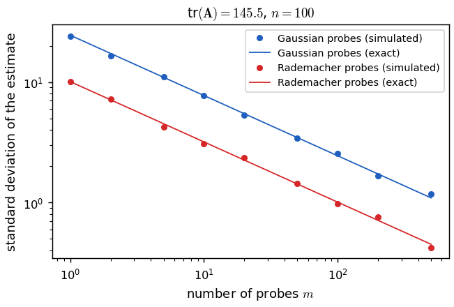
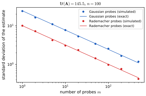
\[ \tr(\A)=\tr(\A\E[\v\v^\T])=\E[\tr(\A\v\v^\T)]=\E[\tr(\v^\T\A\v)]=\E[\v^\T\A\v], \tag{7.37} \]so averaging \(\v_j^\T\A\v_j\) over \(m\) independent probes estimates \(\tr\A\) using only products \(\A\v\). The book does not say how accurate this is; the next box does, and Figure 7.S2 below confirms it.
See also (companion course): trace identities and expected quadratic forms (the cyclic property is proved there).
Filling the gap 7.6: the trace facts, and the variance of the Hutchinson estimator pp. 236–237, (7.33)–(7.37)
Derivation
Cyclicity. For \(\A\in\R^{m\times n}\), \(\B\in\R^{n\times m}\), \(\tr(\A\B)\)\({}=\sum_i\sum_kA_{ik}B_{ki}\)\({}=\sum_k\sum_iB_{ki}A_{ik}\)\({}=\tr(\B\A)\) (7.33); the products need not have the same size. (7.35) is (7.33) with \(\A\) and \(\B\mathbf C\). The trace trick (7.36) is (7.33) with \(\x^\T\) and \(\A\x\), since a scalar equals its trace.
Trace = sum of eigenvalues (7.34). The characteristic polynomial \(\det(\lambda\I-\A)\)\({}=\prod_i(\lambda-\lambda_i)\) (over \(\mathbb C\), with multiplicities). Expanding the determinant (Leibniz formula, Gap 7.7), only the product of the diagonal entries \(\prod_i(\lambda-A_{ii})\) contributes to the coefficient of \(\lambda^{n-1}\), because any other permutation misses at least two diagonal entries. That coefficient is \(-\sum_iA_{ii}\) on one side and \(-\sum_i\lambda_i\) on the other. (Setting \(\lambda=0\) similarly gives \(\det\A=\prod_i\lambda_i\), (7.43).)
Unbiasedness (7.37). Linearity of trace and expectation; only \(\E[\v\v^\T]=\I\) is needed (Gaussian \(\N(\mathbf 0,\I)\) probes, or Rademacher probes with independent \(\pm1\) entries).
Variance. Only the symmetric part \(\A_s=\tfrac12(\A+\A^\T)\) matters, since \(\v^\T\A\v=\v^\T\A_s\v\) (7.57). Write \(\A_s=\mathbf Q\Lam\mathbf Q^\T\). (a) Gaussian probes. \(\mathbf z=\mathbf Q^\T\v\sim\N(\mathbf 0,\I)\), so \(\v^\T\A_s\v=\sum_i\lambda_iz_i^2\) is a weighted sum of independent \(\chi^2_1\) variables, each of variance 2: \(\var(\v^\T\A\v)\)\({}=2\sum_i\lambda_i^2\)\({}=2\|\A_s\|_F^2\). (b) Rademacher probes. \(\v^\T\A_s\v\)\({}=\sum_ia_{ii}+\sum_{i\ne j}a_{ij}v_iv_j\) because \(v_i^2=1\). The products \(v_iv_j\) (\(i\lt j\)) have mean 0, variance 1, and are pairwise uncorrelated, so \(\var\)\({}=4\sum_{i\lt j}a_{ij}^2\)\({}=2\big(\|\A_s\|_F^2-\sum_ia_{ii}^2\big)\). With \(m\) independent probes the variances are divided by \(m\). Rademacher probes are never worse, and are exact for a diagonal matrix. For the \(100\times100\) matrix of Figure 7.S2 the single-probe standard deviations are 24.4 (Gaussian) and 10.1 (Rademacher), for a trace of 145.5. ∎
7.1.4.2 Determinant of a square matrix
p. 237, (7.38)–(7.45) The determinant measures how the linear map changes volume. The book skips the definition; its properties are
\[ |\A|=|\A^\T|,\quad |c\A|=c^n|\A|,\quad |\A\B|=|\A||\B|,\quad |\A|=0\iff\A\text{ singular},\quad |\A^{-1}|=1/|\A|,\quad |\A|=\prod_i\lambda_i, \tag{7.38--7.43} \]and, for positive definite \(\A=\mathbf L\mathbf L^\T\) (Cholesky, Section 7.6.3),
\[ \det(\A)=\det(\mathbf L)^2,\qquad \log\det(\A)=2\sum_i\log L_{ii}=2\tr(\log(\diag(\mathbf L))). \tag{7.44, 7.45} \]The last formula is how log-determinants of covariance matrices are computed in practice: it never forms the determinant itself, which overflows or underflows for moderate \(n\) (the function logdet_chol in the code).
Filling the gap 7.7: what the determinant is, and why (7.38)–(7.43) hold p. 237
Derivation
Definition. \(\det\) is the unique function of the columns \(\mathbf a_1,\dots,\mathbf a_n\) that is (a) linear in each column separately, (b) alternating (zero when two columns are equal, hence it changes sign when two columns are swapped), and (c) equal to 1 at \(\I\). Expanding each column in the standard basis and using (a)–(c) gives the Leibniz formula
\[ \det\A=\sum_{\pi\in S_n}\sgn(\pi)\prod_{i=1}^nA_{\pi(i),i}, \]which proves uniqueness, and one checks directly that this formula has (a)–(c), which proves existence. For \(n=2\) it is \(ad-bc\).
Properties. (7.38): substitute \(\pi\to\pi^{-1}\) in the Leibniz sum (\(\sgn\pi^{-1}=\sgn\pi\)). (7.39): \(n\) columns each scaled by \(c\), by (a). (7.40): for fixed \(\A\), \(\B\mapsto\det(\A\B)\) is multilinear and alternating in the columns of \(\B\) (column \(j\) of \(\A\B\) is \(\A\mathbf b_j\)), so it equals \(\det(\A\B)=\det(\A\I)\det\B\) by uniqueness up to the value at \(\I\). (7.41): if the columns are dependent, one column is a combination of the others and multilinearity plus (b) give 0; if \(\A\) is invertible, (7.40) gives \(\det\A\det\A^{-1}=1\), so \(\det\A\ne0\) and (7.42). (7.43): constant coefficient of the characteristic polynomial, as in Gap 7.6. Triangular matrices: in the Leibniz sum only the identity permutation avoids a zero factor, so \(\det\) is the product of the diagonal (used in Section 7.1.5.2).
Volume. Gaussian elimination writes \(\A\) as a product of elementary matrices (shears, which preserve volume and have determinant 1; axis scalings by \(c\), determinant \(c\); swaps, determinant \(-1\)). Each multiplies the volume of any region by \(|\det|\), so \(\A\) maps the unit cube to a parallelepiped of volume \(|\det\A|\); the sign records whether orientation is reversed.
(7.44)–(7.45). \(\det\mathbf L=\prod_iL_{ii}\) (triangular) and \(L_{ii}>0\), so \(\log\det\A=2\sum_i\log L_{ii}\). ∎
7.1.4.3 Rank of a matrix
pp. 237–238 The column rank is \(\dim\range(\A)\), the row rank \(\dim\range(\A^\T)\); they are equal, and the common value is \(\rank(\A)\). The book lists, without proof: \(\rank\A\le\min(m,n)\) (full rank when equal); \(\rank\A\)\({}=\rank\A^\T\)\({}=\rank(\A^\T\A)\)\({}=\rank(\A\A^\T)\); \(\rank(\A\B)\le\min(\rank\A,\rank\B)\); \(\rank(\A+\B)\le\rank\A+\rank\B\); and a square matrix is invertible iff it has full rank.
Filling the gap 7.8: row rank equals column rank, and the other rank facts pp. 237–238
Derivation
Row rank = column rank. Let \(r\) be the column rank and let the columns of \(\mathbf C\in\R^{m\times r}\) be a basis of \(\range(\A)\). Each column of \(\A\) is a combination of them: \(\A=\mathbf C\mathbf F\) for some \(\mathbf F\in\R^{r\times n}\). Then every row of \(\A\) is a combination of the \(r\) rows of \(\mathbf F\), so row rank \(\le r\). Applying this to \(\A^\T\) gives the reverse inequality. (The SVD gives a second proof in Section 7.5.4.)
\(\rank\A\le\min(m,n)\): the range is a subspace of \(\R^m\) spanned by \(n\) vectors (Gap 7.1).
\(\rank(\A^\T\A)=\rank\A\). \(\nullsp(\A^\T\A)=\nullsp(\A)\): if \(\A^\T\A\x=\mathbf 0\) then \(\|\A\x\|^2=\x^\T\A^\T\A\x=0\). Both matrices have \(n\) columns, so by rank–nullity (Gap 7.2) they have the same rank. Applied to \(\A^\T\), \(\rank(\A\A^\T)=\rank\A^\T=\rank\A\).
Products. \(\range(\A\B)\subseteq\range(\A)\), so \(\rank(\A\B)\le\rank\A\); and \(\rank(\A\B)\)\({}=\rank(\B^\T\A^\T)\)\({}\le\rank\B^\T\)\({}=\rank\B\).
Sums. \(\range(\A+\B)\subseteq\range\A+\range\B\), whose dimension is at most \(\rank\A+\rank\B\).
Invertibility. A square \(\A\) of full rank \(n\) has \(\range\A=\R^n\) and \(\nullsp\A=\{\mathbf 0\}\), so \(\x\mapsto\A\x\) is a bijection; its inverse is linear, hence a matrix \(\A^{-1}\). Conversely, \(\A^{-1}\A=\I\) gives \(n=\rank\I\le\rank\A\). ∎
7.1.4.4 Condition numbers
pp. 238–239, (7.46)–(7.51) The condition number of an invertible matrix is
\[ \kappa(\A)\triangleq\|\A\|\cdot\|\A^{-1}\|, \tag{7.46} \]and in the 2-norm \(\kappa(\A)\)\({}=\sigma_{\max}/\sigma_{\min}\)\({}=\sqrt{\lambda_{\max}/\lambda_{\min}}\) (eigenvalues of \(\A^\T\A\)) (7.51). If \(\A\x=\b\) and \(\b\) changes to \(\b+\Delta\b\), the solution changes by \(\Delta\x=\A^{-1}\Delta\b\) (7.47), (7.48). The book's example
\[ \A=\tfrac12\begin{pmatrix}1&1\\1+10^{-10}&1-10^{-10}\end{pmatrix},\qquad \A^{-1}=\begin{pmatrix}1-10^{10}&10^{10}\\1+10^{10}&-10^{10}\end{pmatrix} \tag{7.49} \]has solution \(\x=(1,1)\) for \(\b=(1,1)\), but
\[ \Delta\x=\big(\Delta b_1-10^{10}(\Delta b_1-\Delta b_2),\ \Delta b_1+10^{10}(\Delta b_1-\Delta b_2)\big): \tag{7.50} \]a change of \(10^{-10}\) in one entry of \(\b\) moves \(\x\) by about 1. I computed \(\kappa(\A)=2.0000\times10^{10}\), confirming the book's value, while \(|\det\A|=5\times10^{-11}\). The book also notes that \(0.1\I_{100}\) has determinant \(10^{-100}\) yet \(\kappa=1\): the determinant is a poor measure of nearness to singularity, the condition number a good one.
Filling the gap 7.9: \(\kappa\ge1\), the perturbation bound, and \(\kappa\) as distance to singularity pp. 238–239
Derivation
\(\kappa\ge1\). For any induced norm \(\|\I\|=1\), and submultiplicativity (Gap 7.5) gives \(1=\|\A\A^{-1}\|\le\|\A\|\,\|\A^{-1}\|\).
The relative error bound. From \(\b=\A\x\), \(\|\b\|\le\|\A\|\,\|\x\|\); from \(\Delta\x=\A^{-1}\Delta\b\), \(\|\Delta\x\|\le\|\A^{-1}\|\,\|\Delta\b\|\). Dividing,
\[ \frac{\|\Delta\x\|}{\|\x\|}\ \le\ \kappa(\A)\,\frac{\|\Delta\b\|}{\|\b\|}. \]The bound is attained in the 2-norm: take \(\b=\sigma_1\u_1\) (so \(\x=\v_1\)) and \(\Delta\b=\epsilon\u_n\) (so \(\Delta\x=(\epsilon/\sigma_n)\v_n\)); the ratio of relative changes is \(\sigma_1/\sigma_n\). A perturbation \(\Delta\A\) of the matrix gives, to first order, \(\|\Delta\x\|/\|\x\|\lesssim\kappa(\A)\|\Delta\A\|/\|\A\|\). In floating point (unit roundoff \(\epsilon\approx1.1\times10^{-16}\)) a backward-stable solver therefore loses about \(\log_{10}\kappa\) of the 16 significant digits.
The 2-norm formula (7.51). \(\|\A\|_2=\sigma_1\) (Gap 7.5) and \(\A^{-1}=\V\mathbf S^{-1}\U^\T\) has largest singular value \(1/\sigma_n\).
Distance to singularity. \(\min\{\|\Delta\A\|_2:\A+\Delta\A\text{ singular}\}\)\({}=\sigma_n\), so \(1/\kappa(\A)=\sigma_n/\sigma_1\) is the relative distance from \(\A\) to the nearest singular matrix (Eckart–Young, Result 7.5, with \(K=n-1\)). For the example (7.49), \(\A\) is within \(5\times10^{-11}\) (relative) of a singular matrix; for \(0.1\I\), the nearest singular matrix is at relative distance 1. ∎
The level sets of \(f(\x)=\x^\T\A\x\) are ellipses whose axis ratio is \(\sqrt{\kappa}\) for symmetric positive definite \(\A\) (Section 7.4.4): a large condition number means a long narrow valley, which is what slows gradient descent (Chapter 8). See the step size versus condition number demonstration of the companion course, and Figure 7.S4 below for what conditioning does to least squares.
7.1.5 Special types of matrices
pp. 239–240, (7.52)–(7.55) A diagonal matrix \(\mathbf D=\diag(d_1,\dots,d_n)\) (7.52); the identity satisfies \(\A\I=\A=\I\A\) (7.53); block diagonal matrices (7.54); band matrices with bandwidth \(k\), e.g. tridiagonal (7.55), for which linear systems are solved in \(O(nk^2)\) instead of \(O(n^3)\) operations. An upper (lower) triangular matrix is zero below (above) the diagonal; its eigenvalues are its diagonal entries, because \(\lambda\I-\A\) is triangular and its determinant is \(\prod_i(\lambda-A_{ii})\) (Gap 7.7).
7.1.5.3 Positive definite matrices
Definition 7.2 (definiteness) pp. 240–241, (7.56)–(7.58)
The quadratic form of \(\A\) is \(\x^\T\A\x=\sum_{i,j}A_{ij}x_ix_j\) (7.56); since \(\x^\T\A\x=\x^\T(\tfrac12\A+\tfrac12\A^\T)\x\) (7.57) only the symmetric part matters, so \(\A\) is taken symmetric. \(\A\in\mathbb S^n\) is positive definite (\(\A\succ0\)) if \(\x^\T\A\x>0\) for all \(\x\ne\mathbf 0\), positive semidefinite (\(\A\succeq0\)) if \(\x^\T\A\x\ge0\), negative (semi)definite if \(-\A\) is positive (semi)definite, and indefinite otherwise. \(\mathbb S^n_{++}\) is the set of positive definite matrices.
The book's examples: \(\begin{pmatrix}4&3\\3&2\end{pmatrix}\) has positive entries but determinant \(-1\lt0\), so one eigenvalue is negative and it is indefinite (\(\x=(1,-1.5)\) gives \(\x^\T\A\x=-0.5\)); \(\begin{pmatrix}2&-1\\-1&2\end{pmatrix}\) has eigenvalues 1 and 3 and is positive definite despite its negative entries. The book also states that definite matrices are invertible, that diagonal dominance (7.58) is sufficient, the \(2\times2\) criterion, and that Gram matrices are positive (semi)definite. Diagonal dominance needs one more hypothesis.
Filling the gap 7.10: invertibility, diagonal dominance (with positive diagonal), the \(2\times2\) test and Gram matrices pp. 240–241
Derivation
Definite implies invertible. If \(\A\x=\mathbf 0\) with \(\x\ne\mathbf 0\), then \(\x^\T\A\x=0\), contradicting definiteness.
Diagonal dominance. Gershgorin's theorem: every eigenvalue \(\lambda\) of \(\A\) lies in some disc \(|\lambda-a_{ii}|\le\sum_{j\ne i}|a_{ij}|\). Proof: if \(\A\x=\lambda\x\), pick \(i\) with \(|x_i|=\max_j|x_j|>0\); row \(i\) gives \((\lambda-a_{ii})x_i=\sum_{j\ne i}a_{ij}x_j\), so \(|\lambda-a_{ii}|\)\({}\le\sum_{j\ne i}|a_{ij}||x_j|/|x_i|\)\({}\le\sum_{j\ne i}|a_{ij}|\). If \(\A\) is symmetric (real eigenvalues), strictly diagonally dominant (7.58) and has positive diagonal entries, each disc lies in \((0,\infty)\), so all eigenvalues are positive and \(\A\succ0\) (Section 7.4.3.1). The book's condition (7.58) uses \(|a_{ii}|\) and omits the sign: \(\begin{pmatrix}-2&1\\1&-2\end{pmatrix}\) is strictly diagonally dominant and negative definite.
The \(2\times2\) test. For \(\A=\begin{pmatrix}a&b\\b&d\end{pmatrix}\), completing the square with \(a\ne0\) gives
\[ ax_1^2+2bx_1x_2+dx_2^2=a\Big(x_1+\frac bax_2\Big)^2+\frac{ad-b^2}a\,x_2^2 . \]If \(a>0\) and \(ad>b^2\) both terms are \(\ge0\) and vanish together only at \(\x=\mathbf 0\). Conversely \(\A\succ0\) needs \(a=\mathbf e_1^\T\A\mathbf e_1>0\) and \(ad-b^2=\det\A=\lambda_1\lambda_2>0\); then \(d>b^2/a\ge0\) automatically. (The general version is Sylvester's criterion: all leading principal minors positive; it follows from the Cholesky construction of Gap 7.30.)
Gram matrices. \(\x^\T\A^\T\A\x=\|\A\x\|^2\ge0\), so \(\A^\T\A\succeq0\) for every \(\A\). It is positive definite iff \(\A\x\ne\mathbf 0\) for \(\x\ne\mathbf 0\), i.e. iff the columns of \(\A\) are independent (\(\rank\A=n\), which needs \(m\ge n\)). ∎
7.1.5.4 Orthogonal matrices
pp. 241–242, (7.59)–(7.64) A square \(\U\) with orthonormal columns is orthogonal: \(\U^\T\U=\I=\U\U^\T\) (7.59). A rectangular \(\U\in\R^{m\times n}\) (\(n\lt m\)) with orthonormal columns has \(\U^\T\U=\I_n\) but \(\U\U^\T\ne\I_m\) (it is the projection onto its range). The rotation by \(\alpha\) about the \(z\) axis,
\[ \mathbf R(\alpha)=\begin{pmatrix}\cos\alpha&-\sin\alpha&0\\ \sin\alpha&\cos\alpha&0\\0&0&1\end{pmatrix}, \tag{7.60} \]is orthogonal, with \(\mathbf R(-\alpha)\)\({}=\mathbf R(\alpha)^{-1}\)\({}=\mathbf R(\alpha)^\T\) ((7.61) is the case \(\alpha=45^\circ\)). Orthogonal maps preserve length, \(\|\U\x\|_2=\|\x\|_2\) (7.62), and angle, \(\cos\alpha(\U\x,\U\y)=\cos\alpha(\x,\y)\) with \(\cos\alpha(\x,\y)=\x^\T\y/(\|\x\|\|\y\|)\) (7.63), (7.64); they are rotations (\(\det\U=1\)) or reflections composed with rotations (\(\det\U=-1\)).
Filling the gap 7.11: one-sided orthogonality suffices for square matrices; norms, angles and determinants pp. 241–242
Derivation
\(\U^\T\U=\I\Rightarrow\U\U^\T=\I\) for square \(\U\). \(\U^\T\U=\I\) says \(\U^\T\) is a left inverse; a square matrix with a left inverse is invertible (rank argument of Gap 7.8), and then the left inverse equals the inverse: \(\U^\T\)\({}=\U^\T(\U\U^{-1})\)\({}=(\U^\T\U)\U^{-1}\)\({}=\U^{-1}\). So the rows are orthonormal too. The argument fails for rectangular \(\U\), where \(\U\U^\T\) has rank \(n\lt m\).
Lengths and angles. \(\|\U\x\|^2=\x^\T\U^\T\U\x=\x^\T\x\) and \((\U\x)^\T(\U\y)=\x^\T\y\); (7.64) follows. These hold also for rectangular \(\U\) with \(\U^\T\U=\I\).
Determinant. \(1=\det(\U^\T\U)=(\det\U)^2\). Conversely, a linear map preserving lengths preserves inner products (polarisation, \(\x^\T\y=\tfrac14(\|\x+\y\|^2-\|\x-\y\|^2)\)), so its matrix satisfies \(\U^\T\U=\I\).
The rotation. The columns of \(\mathbf R(\alpha)\) have squared lengths \(\cos^2\alpha+\sin^2\alpha=1\) and 1, and the first two are orthogonal: \(-\cos\alpha\sin\alpha+\sin\alpha\cos\alpha=0\). This is Exercise 7.1(a), worked out in full in the solution. ∎
The book mentions Gram–Schmidt orthogonalisation as "a way to make any square matrix orthogonal". More precisely it turns linearly independent columns into orthonormal ones spanning the same nested subspaces; it is the QR factorisation of Section 7.6.2 (Gap 7.29).
7.2 Matrix multiplication
p. 242, (7.65), (7.66) For \(\A\in\R^{m\times n}\), \(\B\in\R^{n\times p}\), \(\mathbf C=\A\B\in\R^{m\times p}\) has \(C_{ij}=\sum_kA_{ik}B_{kj}\). This costs \(mnp\) multiplications. The product is associative (\((\A\B)\mathbf C=\A(\B\mathbf C)\): both have entries \(\sum_{k,l}A_{ik}B_{kl}C_{lj}\)) and distributive, but not commutative: \(\begin{pmatrix}0&1\\0&0\end{pmatrix}\begin{pmatrix}0&0\\1&0\end{pmatrix}=\begin{pmatrix}1&0\\0&0\end{pmatrix}\) while the product in the other order is \(\begin{pmatrix}0&0\\0&1\end{pmatrix}\).
7.2.1–7.2.3 Vector–vector, matrix–vector and matrix–matrix products
pp. 242–245, (7.67)–(7.74) The inner product \(\langle\x,\y\rangle=\x^\T\y=\sum_ix_iy_i\) (7.67) is a scalar; the outer product \(\x\y^\T\) (7.68) is an \(m\times n\) matrix of rank one. A matrix–vector product can be read by rows, \(y_i=\mathbf a_i^\T\x\) (7.69), or by columns, \(\A\x=\sum_jx_j\A_{:,j}\) (7.70), a combination of the columns: the second reading is why \(\range(\A)\) is the span of the columns. A matrix product has four readings: entries as inner products of rows and columns (7.71); a sum of outer products \(\A\B=\sum_k\A_{:,k}\B_{k,:}\) (7.72); columns \(\mathbf c_j=\A\mathbf b_j\) (7.73); rows \(\mathbf c_i^\T=\mathbf a_i^\T\B\) (7.74). All four are the same double sum grouped differently. The outer-product reading (7.72) is the one behind the SVD expansion \(\A=\sum_k\sigma_k\u_k\v_k^\T\) (7.178), the truncated SVD and the scatter matrix (7.83). Figure 7.5 is a schematic and is not reproduced.
Notation: \(\A^2=\A\A\), while \(\A^{\odot2}=[A_{ij}^2]\) squares entrywise; \(\sqrt{\mathbf M}\) denotes a matrix with \(\A^2=\mathbf M\) (for \(\mathbf M\succeq0\) the symmetric positive semidefinite one is unique: \(\U\Lam^{1/2}\U^\T\)).
7.2.4 Application: manipulating data matrices
pp. 245–247, (7.75)–(7.94) For a data matrix \(\X\in\R^{N\times D}\) with rows \(\x_n^\T\): column sums \(\mathbf 1_N^\T\X\) (7.75), the mean \(\bar\x^\T=\frac1N\mathbf 1_N^\T\X\) (7.76), row sums \(\X\mathbf 1_D\) (7.77), the total \(\mathbf 1_N^\T\X\mathbf 1_D\) (7.78), (7.79). Pre-multiplying by \(\diag(\mathbf s)\) scales the rows (7.80), post-multiplying scales the columns (7.81), so standardisation is
\[ \operatorname{standardize}(\X)=(\X-\mathbf 1_N\bm\mu^\T)\diag(\bm\sigma)^{-1}. \tag{7.82} \]The sum-of-squares matrix and the scatter matrix are
\[ \mathbf S_0\triangleq\X^\T\X=\sum_n\x_n\x_n^\T,\qquad \mathbf S_{\bar x}\triangleq\sum_n(\x_n-\bar\x)(\x_n-\bar\x)^\T=\Big(\sum_n\x_n\x_n^\T\Big)-N\bar\x\bar\x^\T, \tag{7.83, 7.84} \]and with the centring matrix \(\mathbf C_N=\I_N-\frac1N\mathbf J_N\), \(\mathbf J_N=\mathbf 1_N\mathbf 1_N^\T\),
\[ \tilde\X=\X-\mathbf 1_N\bar\x^\T=\mathbf C_N\X,\qquad \mathbf S_{\bar x}=\tilde\X^\T\tilde\X=\X^\T\mathbf C_N\X. \tag{7.85--7.87} \]For the Gram matrix \(\mathbf K=\X\X^\T\) (7.88), with entries \(\x_i^\T\x_j\), the centred version is obtained by double centring, which needs only \(\mathbf K\) (used by kernel PCA and classical multidimensional scaling):
\[ \tilde{\mathbf K}=\tilde\X\tilde\X^\T=\mathbf C_N\mathbf K\mathbf C_N=\mathbf K-\tfrac1N\mathbf J\mathbf K-\tfrac1N\mathbf K\mathbf J+\tfrac1{N^2}(\mathbf 1^\T\mathbf K\mathbf 1)\mathbf J. \tag{7.89} \](The book prints the last term as the scalar \(\frac1{N^2}\mathbf 1^\T\mathbf K\mathbf 1\), to be read as added to every entry; written as a matrix it is \(\frac1{N^2}(\mathbf 1^\T\mathbf K\mathbf 1)\mathbf J=\frac1{N^2}\mathbf J\mathbf K\mathbf J\).) Finally, the squared distances between the rows of \(\X\in\R^{N_x\times D}\) and \(\mathbf Y\in\R^{N_y\times D}\) are
\[ D_{ij}=\|\x_i\|^2-2\x_i^\T\y_j+\|\y_j\|^2,\qquad \mathbf D=\hat\x\mathbf 1_{N_y}^\T-2\X\mathbf Y^\T+\mathbf 1_{N_x}\hat\y^\T, \tag{7.92, 7.93} \]with \(\hat\x=\diag(\X\X^\T)\) the vector of squared norms; (7.94) is the case \(\mathbf Y=\X\). One matrix product replaces a double loop.
Filling the gap 7.12: the centring matrix, double centring and the distance formula pp. 246–247, (7.84)–(7.94)
Derivation
(7.84). Expand:
\[ \sum_n(\x_n-\bar\x)(\x_n-\bar\x)^\T=\sum_n\x_n\x_n^\T-\Big(\sum_n\x_n\Big)\bar\x^\T-\bar\x\sum_n\x_n^\T+N\bar\x\bar\x^\T, \]and \(\sum_n\x_n=N\bar\x\).
\(\mathbf C_N\) is a symmetric idempotent. \(\mathbf J^2\)\({}=\mathbf 1(\mathbf 1^\T\mathbf 1)\mathbf 1^\T\)\({}=N\mathbf J\), so \(\mathbf C_N^2\)\({}=\I-\frac2N\mathbf J+\frac1{N^2}N\mathbf J\)\({}=\mathbf C_N\). It is the orthogonal projection onto \(\mathbf 1^\perp\) (Gap 7.3 with \(\A=\mathbf 1\)): its eigenvalues are 0 (eigenvector \(\mathbf 1\)) and 1 (multiplicity \(N-1\)), which is why the scatter matrix has rank at most \(N-1\). Then \(\tilde\X\)\({}=\X-\frac1N\mathbf 1\mathbf 1^\T\X\)\({}=\mathbf C_N\X\) and \(\tilde\X^\T\tilde\X\)\({}=\X^\T\mathbf C_N^\T\mathbf C_N\X\)\({}=\X^\T\mathbf C_N\X\) (7.87).
(7.89). \(\tilde\X\tilde\X^\T\)\({}=\mathbf C_N\X\X^\T\mathbf C_N\)\({}=(\I-\tfrac1N\mathbf J)\mathbf K(\I-\tfrac1N\mathbf J)\); expanding gives \(\mathbf K-\frac1N\mathbf J\mathbf K-\frac1N\mathbf K\mathbf J+\frac1{N^2}\mathbf J\mathbf K\mathbf J\), and \(\mathbf J\mathbf K\mathbf J\)\({}=\mathbf 1(\mathbf 1^\T\mathbf K\mathbf 1)\mathbf 1^\T\)\({}=(\mathbf 1^\T\mathbf K\mathbf 1)\mathbf J\). In entries: \(\tilde K_{ij}\)\({}=K_{ij}-\bar K_{i\cdot}-\bar K_{\cdot j}+\bar K_{\cdot\cdot}\) (row mean, column mean, grand mean), which is (7.91); the book's (7.90) should read \((\x_i-\bar\x)^\T(\x_j-\bar\x)\). Every row and column of \(\tilde{\mathbf K}\) sums to zero because \(\mathbf C_N\mathbf 1=\mathbf 0\).
(7.92)–(7.93). \((\x_i-\y_j)^\T(\x_i-\y_j)\)\({}=\x_i^\T\x_i-2\x_i^\T\y_j+\y_j^\T\y_j\); the matrix \(\hat\x\mathbf 1^\T\) has \((i,j)\) entry \(\|\x_i\|^2\), \(\mathbf 1\hat\y^\T\) has \(\|\y_j\|^2\). In floating point the formula can return tiny negative numbers for coincident points through cancellation; the code clips at zero. ∎
See also (companion course): the centred kernel matrix in kernel PCA, Bayesian and Probabilistic Machine Learning.
7.2.5 Kronecker products *
p. 248, (7.95)–(7.98) For \(\A\in\R^{m\times n}\), \(\B\in\R^{p\times q}\), the Kronecker product is the \(mp\times nq\) block matrix \(\A\otimes\B=[a_{ij}\B]\) (7.95), (7.96). Two identities:
\[ (\A\otimes\B)^{-1}=\A^{-1}\otimes\B^{-1},\qquad (\A\otimes\B)\vecop(\mathbf C)=\vecop(\B\mathbf C\A^\T), \tag{7.97, 7.98} \]with column-stacking \(\vecop\); with row-stacking the right side is \(\vecop(\A\mathbf C\B^\T)\). The second identity is what makes Kronecker-structured covariances cheap: a \(mp\times mp\) product becomes two small matrix products.
Filling the gap 7.13: the mixed-product rule, (7.97) and (7.98) p. 248
Derivation
Mixed product. \((\A\otimes\B)(\mathbf C\otimes\mathbf D)\)\({}=(\A\mathbf C)\otimes(\B\mathbf D)\) when the products are defined: block \((i,j)\) of the left side is \(\sum_ka_{ik}\B\,c_{kj}\mathbf D\)\({}=(\A\mathbf C)_{ij}\B\mathbf D\).
(7.97) (square invertible \(\A,\B\)): \((\A\otimes\B)(\A^{-1}\otimes\B^{-1})\)\({}=\I\otimes\I\)\({}=\I\). The same rule gives the eigen-structure: if \(\A\u=\lambda\u\) and \(\B\v=\mu\v\), then \((\A\otimes\B)(\u\otimes\v)\)\({}=\lambda\mu(\u\otimes\v)\), so \(\det(\A\otimes\B)=\det(\A)^p\det(\B)^m\) for \(\A\in\R^{m\times m}\), \(\B\in\R^{p\times p}\).
(7.98). Let \(\mathbf C\in\R^{q\times n}\) with columns \(\mathbf c_1,\dots,\mathbf c_n\), so \(\vecop\mathbf C\)\({}=[\mathbf c_1;\dots;\mathbf c_n]\). Block row \(i\) of \((\A\otimes\B)\vecop\mathbf C\) is \(\sum_ja_{ij}\B\mathbf c_j\)\({}=\B\big(\sum_j\mathbf c_ja_{ij}\big)\)\({}=\B\mathbf C(\A^\T)_{:,i}\), the \(i\)th column of \(\B\mathbf C\A^\T\). Stacking these columns is \(\vecop(\B\mathbf C\A^\T)\). With row-major stacking the roles of the two factors swap. I confirmed both forms numerically with NumPy (whose reshape is row-major). ∎
7.2.6 Einstein summation *
pp. 248–249, (7.99)–(7.101) Einstein's convention drops summation signs: an index repeated on the right, or absent from the left, is summed. For a batch of one-hot sequences \(S_{ntk}\) (example \(n\), position \(t\), word \(k\)), an embedding \(W_{kd}\) and a classifier \(V_{dc}\), the logits of the bag-of-words model are
\[ E_{ntd}=\sum_kS_{ntk}W_{kd},\qquad E_{nd}=\sum_k\sum_tS_{ntk}W_{kd},\qquad L_{nc}=\sum_dE_{nd}V_{dc}=\sum_{d,k,t}S_{ntk}W_{kd}V_{dc}, \tag{7.99--7.101} \]written np.einsum("ntk,kd,dc->nc", S, W, V). The point of einsum is that the library may choose the order of the contractions.
Filling the gap 7.14: why the contraction order matters p. 249
Derivation
Evaluating (7.101) as written, a loop over \((n,t,k,d,c)\), costs \(NTKDC\) multiply–adds. Grouping the sums changes the cost without changing the result (associativity and distributivity): (i) contract \(\mathbf W\mathbf V\to M_{kc}\) at cost \(KDC\), then (ii) \(\sum_{t,k}S_{ntk}M_{kc}\) at cost \(NTKC\). For \(N=32\), \(T=50\), \(K=1000\), \(D=64\), \(C=10\) the naive count is \(3.07\times10^9\) and the two-step order \(3.3\times10^7\), about 92 times less (this is the order np.einsum_path returns). Choosing an optimal order for many tensors is the problem of finding a good elimination ordering, NP-hard in general, hence the greedy heuristics mentioned in the book. ∎
7.3 Matrix inversion
7.3.1 The inverse of a square matrix
p. 249, (7.102)–(7.107) The inverse of a square \(\A\) is the matrix with \(\A^{-1}\A=\I=\A\A^{-1}\) (7.102); it exists iff \(\det\A\ne0\), and
\[ (\A^{-1})^{-1}=\A,\qquad (\A\B)^{-1}=\B^{-1}\A^{-1},\qquad (\A^{-1})^\T=(\A^\T)^{-1}\triangleq\A^{-\T}, \tag{7.103--7.105} \] \[ \begin{pmatrix}a&b\\c&d\end{pmatrix}^{-1}=\frac1{ad-bc}\begin{pmatrix}d&-b\\-c&a\end{pmatrix},\qquad \begin{pmatrix}\A&\mathbf 0\\ \mathbf 0&\B\end{pmatrix}^{-1}=\begin{pmatrix}\A^{-1}&\mathbf 0\\ \mathbf 0&\B^{-1}\end{pmatrix}. \tag{7.106, 7.107} \]Filling the gap 7.15: uniqueness, one-sided inverses and the cofactor formula p. 249
Derivation
Uniqueness. If \(\B\A=\I\) and \(\A\mathbf C=\I\), then \(\B=\B(\A\mathbf C)=(\B\A)\mathbf C=\mathbf C\). For square matrices one side suffices: \(\B\A=\I\) gives \(\nullsp\A=\{\mathbf 0\}\), so \(\A\) has full rank and a two-sided inverse (Gap 7.8), which must equal \(\B\).
(7.104), (7.105). \((\B^{-1}\A^{-1})(\A\B)=\I\); and transposing \(\A\A^{-1}=\I\) gives \((\A^{-1})^\T\A^\T=\I\).
Existence iff \(\det\A\ne0\). Necessity is (7.40). Sufficiency: the adjugate \(\operatorname{adj}(\A)_{ij}\)\({}=(-1)^{i+j}\det\A_{(ji)}\), with \(\A_{(ji)}\) the matrix without row \(j\) and column \(i\), satisfies \(\A\,\operatorname{adj}\A=\det(\A)\I\) (the diagonal entries are cofactor expansions of \(\det\A\); the off-diagonal ones are expansions of a determinant with two equal rows, hence zero). So \(\A^{-1}=\operatorname{adj}(\A)/\det\A\); for \(n=2\) this is (7.106). The formula is for theory only: Gaussian elimination costs \(O(n^3)\), cofactor expansion \(O(n!)\). (7.107) is checked by multiplying the blocks. ∎
7.3.2 Schur complements *
Theorem 7.3.1 (inverse of a partitioned matrix) p. 250, (7.108)–(7.112)
Let \(\mathbf M=\begin{pmatrix}\mathbf E&\mathbf F\\ \mathbf G&\mathbf H\end{pmatrix}\) (7.108) be invertible, with \(\mathbf E\) and \(\mathbf H\) square and invertible. Then the Schur complements \(\mathbf M/\mathbf H\triangleq\mathbf E-\mathbf F\mathbf H^{-1}\mathbf G\) (7.111) and \(\mathbf M/\mathbf E\triangleq\mathbf H-\mathbf G\mathbf E^{-1}\mathbf F\) (7.112) are invertible and
\[ \mathbf M^{-1}=\begin{pmatrix}(\mathbf M/\mathbf H)^{-1}&-(\mathbf M/\mathbf H)^{-1}\mathbf F\mathbf H^{-1}\\ -\mathbf H^{-1}\mathbf G(\mathbf M/\mathbf H)^{-1}&\mathbf H^{-1}+\mathbf H^{-1}\mathbf G(\mathbf M/\mathbf H)^{-1}\mathbf F\mathbf H^{-1}\end{pmatrix} \tag{7.109} \] \[ \phantom{\mathbf M^{-1}}=\begin{pmatrix}\mathbf E^{-1}+\mathbf E^{-1}\mathbf F(\mathbf M/\mathbf E)^{-1}\mathbf G\mathbf E^{-1}&-\mathbf E^{-1}\mathbf F(\mathbf M/\mathbf E)^{-1}\\ -(\mathbf M/\mathbf E)^{-1}\mathbf G\mathbf E^{-1}&(\mathbf M/\mathbf E)^{-1}\end{pmatrix}. \tag{7.110} \]The first form needs only \(\mathbf H\) (and \(\mathbf M\)) invertible, the second only \(\mathbf E\).
The book's proof (7.113)–(7.121) block-diagonalises \(\mathbf M\): with the unit block-triangular \(\mathbf X=\begin{pmatrix}\I&-\mathbf F\mathbf H^{-1}\\ \mathbf 0&\I\end{pmatrix}\) and \(\mathbf Z=\begin{pmatrix}\I&\mathbf 0\\ -\mathbf H^{-1}\mathbf G&\I\end{pmatrix}\),
\[ \mathbf X\mathbf M\mathbf Z=\mathbf W=\begin{pmatrix}\mathbf M/\mathbf H&\mathbf 0\\ \mathbf 0&\mathbf H\end{pmatrix},\qquad \mathbf M^{-1}=\mathbf Z\mathbf W^{-1}\mathbf X, \tag{7.115--7.117} \]and multiplying out gives (7.109). The book states the theorem assuming only that \(\mathbf E\) and \(\mathbf H\) are invertible; that is not enough.
Filling the gap 7.16: when the Schur complement is invertible pp. 250–251
Derivation
\(\mathbf X\) and \(\mathbf Z\) are invertible (block triangular with identity diagonal blocks, determinant 1; \(\mathbf X^{-1}\) is \(\mathbf X\) with \(-\mathbf F\mathbf H^{-1}\) replaced by \(+\mathbf F\mathbf H^{-1}\)). So \(\mathbf M\) is invertible iff \(\mathbf W\) is, iff \(\mathbf M/\mathbf H\) is (given \(\mathbf H\) invertible); and \(\det\mathbf M\)\({}=\det(\mathbf M/\mathbf H)\det\mathbf H\) (7.128). The hypothesis "\(\mathbf E\), \(\mathbf H\) invertible" alone does not suffice: \(\mathbf M=\begin{pmatrix}1&1\\1&1\end{pmatrix}\) has \(\mathbf E=\mathbf H=1\) but \(\mathbf M/\mathbf H=0\) and \(\mathbf M\) singular. Under the theorem's hypotheses both complements are invertible because \(\det(\mathbf M/\mathbf H)\)\({}=\det\mathbf M/\det\mathbf H\ne0\) and likewise for \(\mathbf M/\mathbf E\).
Positive definite case. If \(\mathbf M\succ0\), then \(\mathbf H\succ0\) (restrict the quadratic form to vectors \((\mathbf 0,\y)\)) and \(\mathbf M/\mathbf H\succ0\): with \(\mathbf G=\mathbf F^\T\), \(\mathbf W=\mathbf X\mathbf M\mathbf X^\T\) is congruent to \(\mathbf M\). This is why a conditional covariance \(\Sig_{11}-\Sig_{12}\Sig_{22}^{-1}\Sig_{21}\) is always a valid covariance (Section 7.3.5), and it is the induction step in the existence proof of the Cholesky factor (Gap 7.30). ∎
7.3.3 The matrix inversion lemma *
Result 7.2 (matrix inversion lemma, Sherman–Morrison–Woodbury) p. 251, (7.122)–(7.125)
Equating the top-left blocks of (7.109) and (7.110):
\[ (\mathbf E-\mathbf F\mathbf H^{-1}\mathbf G)^{-1}=\mathbf E^{-1}+\mathbf E^{-1}\mathbf F(\mathbf H-\mathbf G\mathbf E^{-1}\mathbf F)^{-1}\mathbf G\mathbf E^{-1}. \tag{7.122} \]With \(\mathbf E=\Sig\) (\(N\times N\) diagonal), \(\mathbf F=\mathbf G^\T=\X\) (\(N\times D\)) and \(\mathbf H^{-1}=-\I\):
\[ (\Sig+\X\X^\T)^{-1}=\Sig^{-1}-\Sig^{-1}\X(\I+\X^\T\Sig^{-1}\X)^{-1}\X^\T\Sig^{-1}, \tag{7.123} \]and with \(\mathbf E=\A\), \(\mathbf F=\u\), \(\mathbf G=\v^\T\), \(\mathbf H=-1\), the Sherman–Morrison formula for a rank-one update:
\[ (\A+\u\v^\T)^{-1}=\A^{-1}-\frac{\A^{-1}\u\v^\T\A^{-1}}{1+\v^\T\A^{-1}\u}. \tag{7.124, 7.125} \]7.3.4 Matrix determinant lemma *
Result 7.3 (determinant of a partitioned matrix; matrix determinant lemma) pp. 251–252, (7.126)–(7.133)
\[ |\mathbf M|=|\mathbf M/\mathbf H|\,|\mathbf H|=|\mathbf M/\mathbf E|\,|\mathbf E|,\qquad |\mathbf E-\mathbf F\mathbf H^{-1}\mathbf G|=|\mathbf H-\mathbf G\mathbf E^{-1}\mathbf F|\,|\mathbf H^{-1}|\,|\mathbf E|, \tag{7.128--7.132} \] \[ |\A+\u\v^\T|=(1+\v^\T\A^{-1}\u)\,|\A|. \tag{7.133} \]Filling the gap 7.17: checking the substitutions, the conditions, and why the lemma saves work pp. 251–252
Derivation
(7.123). With \(\mathbf H=-\I\): \(\mathbf E-\mathbf F\mathbf H^{-1}\mathbf G\)\({}=\Sig+\X\X^\T\) and \(\mathbf H-\mathbf G\mathbf E^{-1}\mathbf F\)\({}=-(\I+\X^\T\Sig^{-1}\X)\); substituting in (7.122) gives (7.123). All inverses exist when \(\Sig\succ0\): \(\I+\X^\T\Sig^{-1}\X\succeq\I\) and \(\Sig+\X\X^\T\succeq\Sig\). Cost: the left side inverts an \(N\times N\) matrix, \(O(N^3)\); the right side needs \(\X^\T\Sig^{-1}\X\) (\(O(ND^2)\), \(\Sig\) diagonal) and a \(D\times D\) inverse, \(O(D^3)\). For \(N\gg D\) this is the difference between a Gaussian process with \(N\) points and a Bayesian linear model with \(D\) features.
(7.125) directly. Multiply \(\A+\u\v^\T\) by the right side and write \(\beta=\v^\T\A^{-1}\u\): \(\I+\u\v^\T\A^{-1}-\frac{\u\v^\T\A^{-1}+\u\beta\v^\T\A^{-1}}{1+\beta}\)\({}=\I\). The formula requires \(1+\beta\ne0\), which is exactly the condition, by (7.133), for \(\A+\u\v^\T\) to be invertible. Each update costs \(O(n^2)\) instead of \(O(n^3)\); recursive least squares and online Gaussian updates use it.
(7.133). Apply (7.132) with \(\mathbf E=\A\), \(\mathbf F=-\u\), \(\mathbf G=\v^\T\), \(\mathbf H=1\): the left side is \(|\A+\u\v^\T|\), the right side \(|1+\v^\T\A^{-1}\u|\cdot1\cdot|\A|\). The general version \(|\A+\mathbf U\mathbf V^\T|\)\({}=|\A|\,|\I+\mathbf V^\T\A^{-1}\mathbf U|\) is proved the same way. Numerically, both lemmas agree with direct inversion and determinants to about \(10^{-13}\) on random matrices. ∎
See also (companion course): the Woodbury identity and the determinant lemma, with a direct verification and the probabilistic PCA application.
7.3.5 Application: deriving the conditionals of an MVN *
pp. 252–253, (7.134)–(7.147) For a joint Gaussian with blocks \(\bm\mu=(\bm\mu_1,\bm\mu_2)\) and \(\Sig=\begin{pmatrix}\Sig_{11}&\Sig_{12}\\ \Sig_{21}&\Sig_{22}\end{pmatrix}\) (7.134), inserting the factorisation (7.118) of \(\Sig^{-1}\) into the exponent splits it into a quadratic form in \(\x_1-\bm\mu_{1|2}\) plus one in \(\x_2-\bm\mu_2\) (7.136)–(7.141), so \(p(\x_1,\x_2)\)\({}=\N(\x_1\given\bm\mu_{1|2},\Sig_{1|2})\,\N(\x_2\given\bm\mu_2,\Sig_{22})\) (7.143) with
\[ \bm\mu_{1|2}=\bm\mu_1+\Sig_{12}\Sig_{22}^{-1}(\x_2-\bm\mu_2),\qquad \Sig_{1|2}=\Sig/\Sig_{22}=\Sig_{11}-\Sig_{12}\Sig_{22}^{-1}\Sig_{21}. \tag{7.144, 7.145} \]The normalising constants match because \(|\Sig|=|\Sig/\Sig_{22}|\,|\Sig_{22}|\) (7.146), (7.147). The book's derivation is complete; the one point to add is that \(\Sig/\Sig_{22}\) is positive definite (Gap 7.16), so the conditional is a proper Gaussian. The same result, with a geometric reading and a demonstration, is Result 3.5 of the Chapter 3 notes; try it in the bivariate Gaussian demo.
7.4 Eigenvalue decomposition (EVD)
7.4.1 Basics
pp. 253–254, (7.148)–(7.153) \(\lambda\) is an eigenvalue of a square \(\A\) with eigenvector \(\u\ne\mathbf 0\) if \(\A\u=\lambda\u\) (7.148). Any non-zero multiple of \(\u\) is again an eigenvector (7.149), so eigenvectors are normalised to unit length (leaving a sign ambiguity). \((\lambda\I-\A)\u=\mathbf 0\) has a non-zero solution iff \(\lambda\I-\A\) is singular, i.e.
\[ \det(\lambda\I-\A)=0, \tag{7.151} \]the characteristic equation, a polynomial equation of degree \(n\) with \(n\) complex roots counted with multiplicity. The book lists: \(\tr\A=\sum_i\lambda_i\) (7.152), \(\det\A=\prod_i\lambda_i\) (7.153), "the rank of \(\A\) equals the number of non-zero eigenvalues", \(\A^{-1}\u_i=\lambda_i^{-1}\u_i\), and that triangular matrices have their diagonal as eigenvalues. The rank statement is false in general.
Filling the gap 7.18: the eigenvalue facts, and when rank equals the number of non-zero eigenvalues p. 254
Derivation
(7.152) and (7.153) were proved in Gap 7.6 from the coefficients of the characteristic polynomial. Inverse: if \(\A\) is invertible, \(\lambda_i\ne0\) (else \(\A\u_i=\mathbf 0\)), and multiplying \(\A\u_i=\lambda_i\u_i\) by \(\lambda_i^{-1}\A^{-1}\) gives \(\A^{-1}\u_i=\lambda_i^{-1}\u_i\). Powers: likewise \(\A^k\u_i=\lambda_i^k\u_i\), the fact behind the power method.
Rank. The nilpotent matrix \(\mathbf N=\begin{pmatrix}0&1\\0&0\end{pmatrix}\) has characteristic polynomial \(\lambda^2\), so both eigenvalues are 0, yet \(\rank\mathbf N=1\). What is true: the rank is at least the number of non-zero eigenvalues (counted with multiplicity), with equality when \(\A\) is diagonalisable, in particular when \(\A\) is symmetric. Proof of the equality: if \(\A=\U\Lam\U^{-1}\), then \(\rank\A=\rank\Lam\) (multiplying by invertible matrices does not change the rank, Gap 7.8), and \(\rank\Lam\) is the number of non-zero diagonal entries. For general \(\A\), the number of zero eigenvalues (algebraic multiplicity of 0) is at least \(\dim\nullsp\A\) (the geometric multiplicity), which gives the inequality by rank–nullity. The rank always equals the number of non-zero singular values (Section 7.5.4). ∎
The book also says that for a rotation matrix the eigenvector is the axis of rotation with \(\lambda=1\). That is the three-dimensional picture (Exercise 7.1(b)); a plane rotation by \(\alpha\notin\pi\mathbb Z\) has no real eigenvector at all (its eigenvalues are \(e^{\pm i\alpha}\)).
7.4.2 Diagonalization
pp. 254–255, (7.154)–(7.156) Collecting the eigenvectors as columns of \(\U\) and the eigenvalues in \(\Lam\), \(\A\U=\U\Lam\) (7.154), (7.155); if the eigenvectors are linearly independent, \(\A=\U\Lam\U^{-1}\) (7.156) and \(\A\) is diagonalisable.
Filling the gap 7.19: when is a matrix diagonalisable? p. 255
Derivation
Distinct eigenvalues give independent eigenvectors. Suppose \(\u_1,\dots,\u_k\) are eigenvectors for distinct \(\lambda_1,\dots,\lambda_k\) and take a shortest non-trivial relation \(\sum_{i\in S}c_i\u_i=\mathbf 0\) (all \(c_i\ne0\)). Applying \(\A-\lambda_j\I\) for some \(j\in S\) gives \(\sum_{i\in S,i\ne j}c_i(\lambda_i-\lambda_j)\u_i\)\({}=\mathbf 0\), a shorter non-trivial relation (the factors \(\lambda_i-\lambda_j\ne0\)); a contradiction unless \(|S|=1\), which is impossible since \(\u_i\ne\mathbf 0\). So an \(n\times n\) matrix with \(n\) distinct eigenvalues is diagonalisable.
Not every matrix is. \(\mathbf N\) of Gap 7.18 has only the eigenvectors \(c\mathbf e_1\); one independent eigenvector cannot fill a \(2\times2\) matrix \(\U\). Real matrices may also need complex eigenvalues (plane rotations). Symmetric matrices have neither problem: next section. ∎
7.4.3 Eigenvalues and eigenvectors of symmetric matrices
Result 7.4 (spectral theorem) p. 255, (7.157)–(7.160)
A real symmetric \(\A\in\mathbb S^n\) has real eigenvalues and an orthonormal basis of eigenvectors: \(\A=\U\Lam\U^\T\) with \(\U\) orthogonal, that is
\[ \A=\U\Lam\U^\T=\sum_{i=1}^n\lambda_i\u_i\u_i^\T, \tag{7.157, 7.158} \]so multiplying by \(\A\) rotates by \(\U^\T\), scales by \(\Lam\) and rotates back. If \(\A\) is invertible, \(\A^{-1}\)\({}=\U\Lam^{-1}\U^\T\)\({}=\sum_i\lambda_i^{-1}\u_i\u_i^\T\) (7.159). With \(\y=\U^\T\x\), \(\x^\T\A\x=\sum_i\lambda_iy_i^2\) (7.160): \(\A\) is positive definite iff all \(\lambda_i>0\), semidefinite iff all \(\lambda_i\ge0\), indefinite iff it has eigenvalues of both signs.
Filling the gap 7.20: proof of the spectral theorem p. 255, "it can be shown"
Derivation
Real eigenvalues. Let \(\A\u=\lambda\u\) with \(\u\in\mathbb C^n\setminus\{\mathbf 0\}\) (a root of (7.151) always exists over \(\mathbb C\)). With \(\u^*\) the conjugate transpose, \(\u^*\A\u=\lambda\u^*\u\). The left side is real: its conjugate is \(\u^*\A^*\u=\u^*\A\u\) because \(\A\) is real and symmetric. And \(\u^*\u=\sum|u_i|^2>0\). So \(\lambda\) is real, and then a real eigenvector exists (take the real or imaginary part of \(\u\), one of which is non-zero, since \(\A-\lambda\I\) is real).
Orthogonality for distinct eigenvalues. If \(\A\u=\lambda\u\), \(\A\v=\mu\v\), then \(\lambda\v^\T\u\)\({}=\v^\T\A\u\)\({}=(\A\v)^\T\u\)\({}=\mu\v^\T\u\), so \(\lambda\ne\mu\) forces \(\v^\T\u=0\).
A full orthonormal basis (induction on \(n\)). \(n=1\) is trivial. Take a real unit eigenvector \(\u_1\) with eigenvalue \(\lambda_1\), and let \(S=\u_1^\perp\), of dimension \(n-1\). \(S\) is invariant: for \(\x\in S\), \(\u_1^\T\A\x\)\({}=(\A\u_1)^\T\x\)\({}=\lambda_1\u_1^\T\x\)\({}=0\). Choose an orthonormal basis \(\mathbf Q\in\R^{n\times(n-1)}\) of \(S\); the matrix of \(\A\) restricted to \(S\) is \(\mathbf Q^\T\A\mathbf Q\), symmetric of size \(n-1\). By induction \(\mathbf Q^\T\A\mathbf Q\)\({}=\mathbf V\Lam'\mathbf V^\T\) with \(\mathbf V\) orthogonal; then the columns of \(\mathbf Q\mathbf V\) are orthonormal eigenvectors of \(\A\) in \(S\) (since \(\A\mathbf Q\mathbf V\)\({}=\mathbf Q\mathbf Q^\T\A\mathbf Q\mathbf V\), using invariance), and together with \(\u_1\) they form \(\U\). Repeated eigenvalues are covered: the theorem gives an orthonormal basis of each eigenspace, though not a unique one.
The rest. (7.158) is the outer-product reading (7.72) of \((\U\Lam)\U^\T\). (7.159): \(\U\Lam\U^\T\cdot\U\Lam^{-1}\U^\T=\I\). (7.160): \(\x^\T\U\Lam\U^\T\x=\y^\T\Lam\y\), and \(\x\mapsto\y=\U^\T\x\) is a bijection, so the sign pattern of the form is that of the \(\lambda_i\) (taking \(\y=\mathbf e_i\) shows each \(\lambda_i\) is a value of the form on a unit vector). ∎
See also (companion courses): the spectral theorem and Rayleigh quotients; eigenvectors in Foundations of Deep Learning, Appendix A.4.
7.4.4 Geometry of quadratic forms
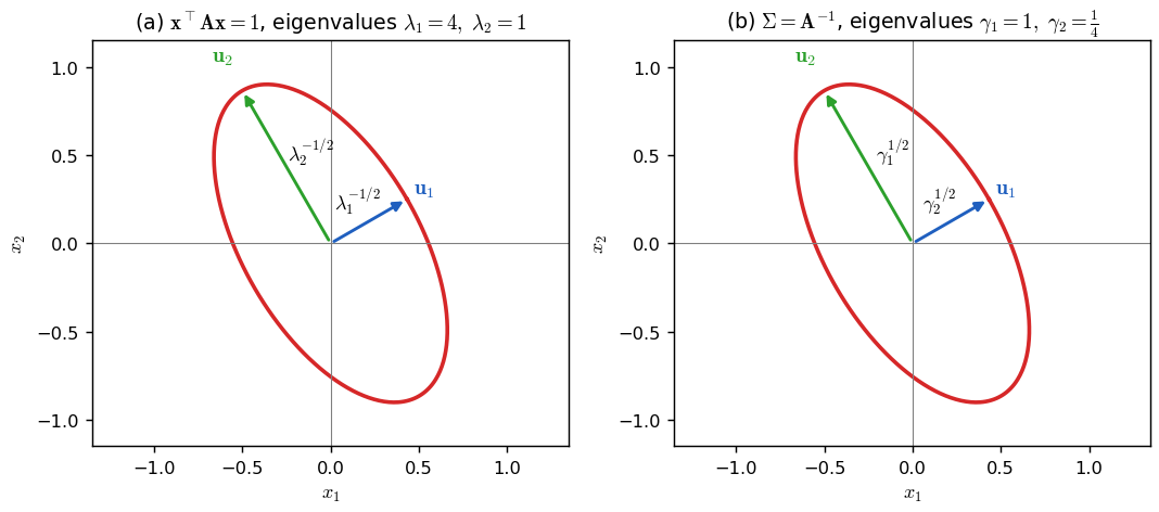
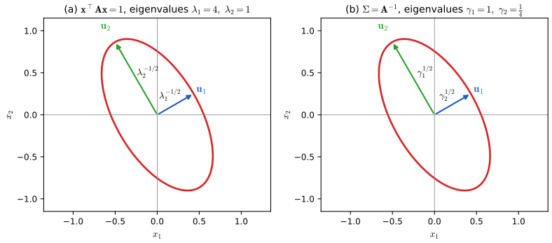
p. 256, (7.161)–(7.163) For \(\A\succ0\) and \(f(\x)=\x^\T\A\x=\sum_i\lambda_iy_i^2\) with \(y_i=\u_i^\T\x\) (7.161), (7.162), the level set \(f=r\) is an ellipsoid; in two dimensions, \(\lambda_1y_1^2+\lambda_2y_2^2=r\) (7.163). Its semi-axes point along \(\u_i\) and have lengths \(\sqrt{r/\lambda_i}\): for \(r=1\), \(a^{-2}=\lambda_1\) and \(b^{-2}=\lambda_2\), so the largest eigenvalue gives the shortest axis. For a Gaussian \(\A=\Sig^{-1}\), and the small eigenvalues of the precision are the directions of large variance. The book's Figure 7.6 labels the semi-axes \(\lambda_i^{1/2}\), which is right when the \(\lambda_i\) are eigenvalues of \(\Sig\) but not, as in the text, of \(\A\); Figure 7.6 below shows both labellings of the same ellipse.
7.4.5 Standardizing and whitening data
pp. 256–258, (7.164)–(7.166) Standardising (7.82) gives unit variances but keeps correlations. Whitening removes them too. Let \(\Sig\)\({}=\frac1N\X^\T\X\)\({}=\mathbf E\mathbf D\mathbf E^\T\) for centred \(\X\) (equivalently \(\mathbf E=\V\), \(\mathbf D=\mathbf S^2\) from the SVD of \(\X/\sqrt N\)). The PCA whitening matrix and its covariance check are
\[ \mathbf W_{\rm pca}=\mathbf D^{-1/2}\mathbf E^\T,\qquad \Cov[\y]=\mathbf W\Sig\mathbf W^\T=(\mathbf D^{-1/2}\mathbf E^\T)(\mathbf E\mathbf D\mathbf E^\T)(\mathbf E\mathbf D^{-1/2})=\I \tag{7.164, 7.165} \]for \(\y=\mathbf W\x\). Any \(\mathbf R\mathbf W_{\rm pca}\) with \(\mathbf R\) orthogonal also whitens; \(\mathbf R=\mathbf E\) gives ZCA (Mahalanobis) whitening (Bell and Sejnowski, 1997)
\[ \mathbf W_{\rm zca}=\mathbf E\mathbf D^{-1/2}\mathbf E^\T=\Sig^{-1/2}=\V\mathbf S^{-1}\V^\T, \tag{7.166} \]which, the book says, keeps the whitened data as close as possible to the original in the least-squares sense; for images it keeps whitened images looking like images. The book does not prove either of the two claims "every whitening matrix is a rotation of \(\mathbf W_{\rm pca}\)" and "ZCA is the closest"; the next box does.
Filling the gap 7.21: all whitening matrices, and the optimality of ZCA pp. 257–258
Derivation
Assume \(\Sig\succ0\) and write \(\Sig^{1/2}\)\({}=\mathbf E\mathbf D^{1/2}\mathbf E^\T\), the symmetric positive definite square root.
Every whitening matrix. \(\mathbf W\Sig\mathbf W^\T=\I\) iff \(\mathbf Q=\mathbf W\Sig^{1/2}\) satisfies \(\mathbf Q\mathbf Q^\T=\I\), i.e. iff \(\mathbf W=\mathbf Q\Sig^{-1/2}\) with \(\mathbf Q\) orthogonal. Since \(\mathbf W_{\rm pca}\)\({}=\mathbf D^{-1/2}\mathbf E^\T\)\({}=\mathbf E^\T\Sig^{-1/2}\), equivalently \(\mathbf W=\mathbf R\mathbf W_{\rm pca}\) with \(\mathbf R=\mathbf Q\mathbf E\) orthogonal. (The book writes the condition as \(\mathbf W^\T\mathbf W=\Sig^{-1}\), which is equivalent for square invertible \(\mathbf W\).)
ZCA is the closest. For centred \(\x\) with covariance \(\Sig\),
\[ \E\|\mathbf W\x-\x\|^2=\tr(\mathbf W\Sig\mathbf W^\T)-2\tr(\mathbf W\Sig)+\tr\Sig=D-2\tr(\mathbf Q\Sig^{1/2})+\tr\Sig. \]So we must maximise \(\tr(\mathbf Q\Sig^{1/2})\)\({}=\tr(\mathbf P\mathbf D^{1/2})\)\({}=\sum_iP_{ii}d_i^{1/2}\) over orthogonal \(\mathbf P=\mathbf E^\T\mathbf Q\mathbf E\). Entries of an orthogonal matrix satisfy \(|P_{ii}|\le1\) (its columns are unit vectors), so the maximum \(\sum_id_i^{1/2}\) is attained iff \(P_{ii}=1\) for all \(i\), i.e. \(\mathbf P=\I\), \(\mathbf Q=\I\), \(\mathbf W=\Sig^{-1/2}=\mathbf W_{\rm zca}\). The minimum displacement is \(\tr\big((\Sig^{1/2}-\I)^2\big)\); in the sample version replace \(\E\) by the average over the data. This is the orthogonal Procrustes problem, and ZCA is its unique solution (Kessy, Lewin and Strimmer, 2018).
Numbers for Figure 7.7. For the 88 men the correlation of height and weight is 0.539; the mean squared displacement is 170.89 for PCA whitening and 147.67 for ZCA, which equals \(\tr((\Sig^{1/2}-\I)^2)\); among all rotations \(\mathbf R(\varphi)\mathbf W_{\rm pca}\) the minimum is at \(\varphi^*=70.2^\circ\), the angle of the first eigenvector. ∎
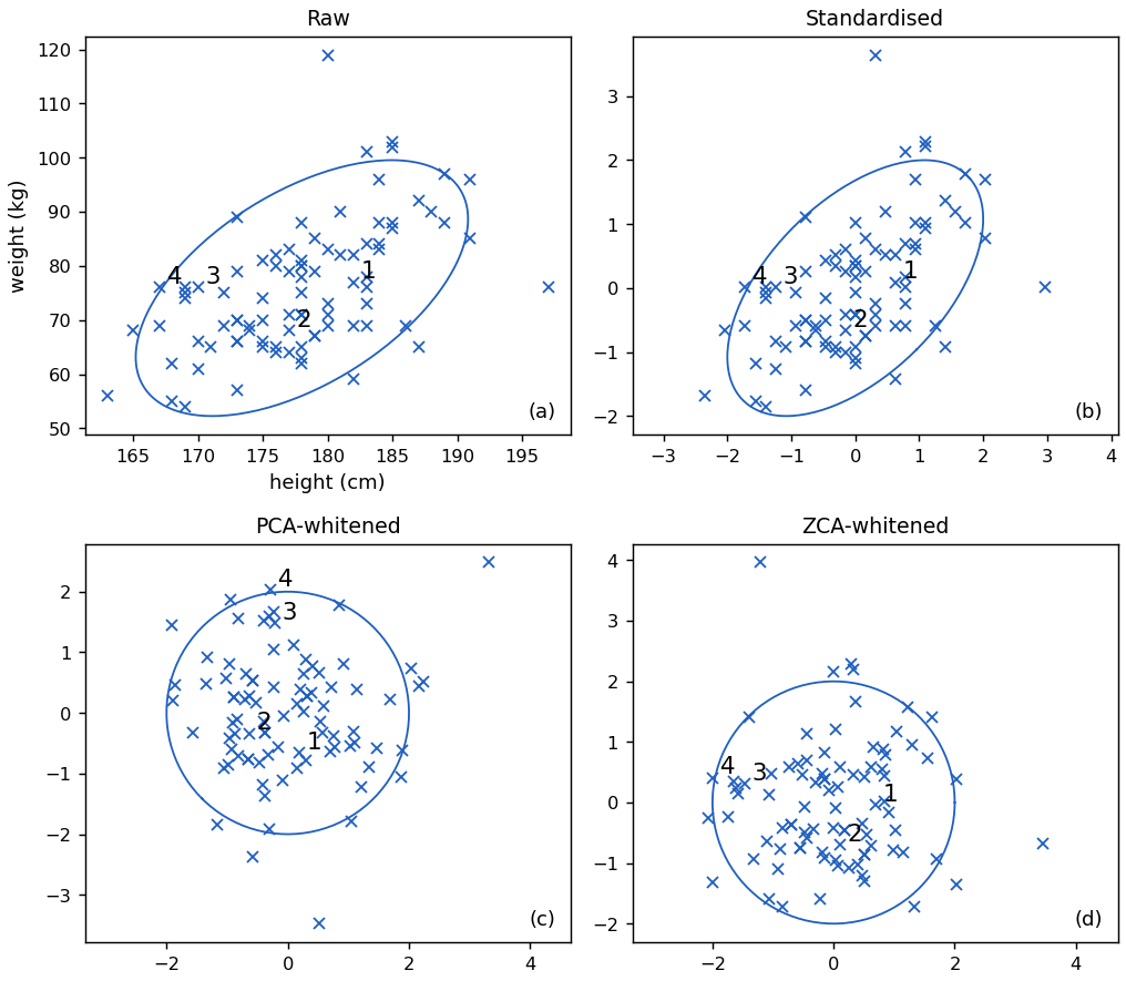
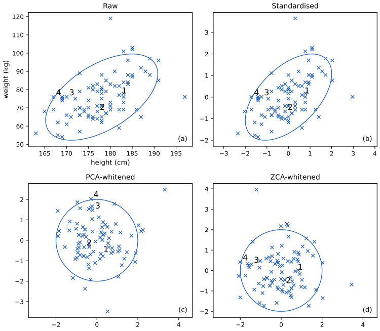
A remark on the book's panel (b): its axes run over about \(\pm0.1\) for height and from \(-1\) to \(1.5\) for weight, so the two columns cannot both have unit variance. The panel looks as if both columns were divided by one pooled standard deviation instead of their own; (7.82) divides each column by its own, as in panel (b) here.
See also (companion course): data whitening in Foundations of Deep Learning.
7.4.6 Power method
p. 258, (7.167)–(7.173) To find the eigenvector of largest-magnitude eigenvalue of a symmetric \(\A\) (with \(|\lambda_1|>|\lambda_2|\ge\dots\)), multiply and renormalise:
\[ \v_t\propto\A\v_{t-1}. \tag{7.168} \]Expanding \(\v_0=\sum_ia_i\u_i\) (7.167), \(\v_t\)\({}\propto\sum_ia_i\lambda_i^t\u_i\)\({}=\lambda_1^t\big(a_1\u_1+\sum_{i\ge2}a_i(\lambda_i/\lambda_1)^t\u_i\big)\)\({}\to\lambda_1^ta_1\u_1\) (7.169)–(7.171), provided \(a_1=\u_1^\T\v_0\ne0\) (true with probability one for a random start). The eigenvalue is read off with the Rayleigh quotient
\[ R(\A,\x)\triangleq\frac{\x^\T\A\x}{\x^\T\x},\qquad R(\A,\u_i)=\lambda_i. \tag{7.172, 7.173} \]The method only needs products \(\A\v\), so it suits large sparse matrices (PageRank). The book takes \(\v_0\) in the range of \(\A\); that is unnecessary. It says the error shrinks by about \(|\lambda_2/\lambda_1|\) per step; the precise statement, and the faster rate of the Rayleigh quotient, are in the next box.
The power method with Rayleigh quotient
Input \(\A\) (only through \(\v\mapsto\A\v\)), start \(\v_0\ne\mathbf 0\), number of steps \(T\). Set \(\v\leftarrow\v_0/\|\v_0\|\). For \(t=1,\dots,T\): \(\mathbf w\leftarrow\A\v\); \(\v\leftarrow\mathbf w/\|\mathbf w\|\); \(\hat\lambda\leftarrow\v^\T\A\v\). Return \((\hat\lambda,\v)\). Cost: \(T\) matrix–vector products. (power_method in the code.)
Filling the gap 7.22: the convergence rate of the power method and of the Rayleigh quotient p. 258, (7.169)–(7.171)
Derivation
Let \(\A=\sum_i\lambda_i\u_i\u_i^\T\) be symmetric with \(|\lambda_1|>|\lambda_2|\)\({}\ge\dots\)\({}\ge|\lambda_n|\), \(\v_0=\sum_ia_i\u_i\) with \(a_1\ne0\), and \(\theta_t\) the angle between \(\v_t\) and the line through \(\u_1\). Since \(\v_t\) is a multiple of \(\A^t\v_0=\sum_ia_i\lambda_i^t\u_i\) and the \(\u_i\) are orthonormal,
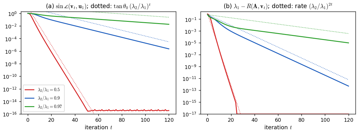
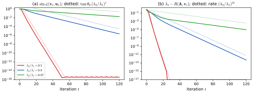
\[ \tan\theta_t=\frac{\big(\sum_{i\ge2}a_i^2\lambda_i^{2t}\big)^{1/2}}{|a_1\lambda_1^t|}\ \le\ \Big|\frac{\lambda_2}{\lambda_1}\Big|^t\frac{\big(\sum_{i\ge2}a_i^2\big)^{1/2}}{|a_1|}=\Big|\frac{\lambda_2}{\lambda_1}\Big|^t\tan\theta_0 . \]So the angle decays geometrically with ratio \(|\lambda_2/\lambda_1|\); the number of steps for accuracy \(\epsilon\) is about \(\log(\tan\theta_0/\epsilon)/\log|\lambda_1/\lambda_2|\), which blows up as the eigengap closes. In two dimensions the bound is an equality.
Rayleigh quotient. With weights \(w_i=a_i^2\lambda_i^{2t}\), \(R(\A,\v_t)=\sum_i\lambda_iw_i/\sum_iw_i\), so
\[ |\lambda_1-R(\A,\v_t)|=\frac{\sum_{i\ge2}|\lambda_1-\lambda_i|\,w_i}{\sum_iw_i}\ \le\ \max_i|\lambda_1-\lambda_i|\ \tan^2\theta_t=O\big(|\lambda_2/\lambda_1|^{2t}\big). \]The eigenvalue converges twice as fast (in digits) as the eigenvector: a Rayleigh quotient is stationary at eigenvectors (Section 7.4.8), so a first-order error in \(\v\) gives a second-order error in \(R\).
Signs and ties. If \(\lambda_1\lt0\), \(\v_t\) alternates in sign but the line converges and \(R\to\lambda_1\). If \(\lambda_2=-\lambda_1\) the ratio is 1 and there is no convergence: \(\A^2\) has a repeated top eigenvalue and the iterates cycle (preset 4 of the demo). If \(a_1=0\) exactly, the iteration converges to the next eigenvector, although rounding errors usually reintroduce a \(\u_1\) component. ∎
7.4.7 Deflation
p. 259, (7.174) Having found \((\lambda_1,\u_1)\), remove it:
\[ \A^{(2)}=(\I-\u_1\u_1^\T)\A^{(1)}=\A^{(1)}-\u_1\u_1^\T\A^{(1)}=\A^{(1)}-\lambda_1\u_1\u_1^\T, \tag{7.174} \]and run the power method on \(\A^{(2)}\) to get \((\lambda_2,\u_2)\). Repeating gives the top \(K\) eigenpairs, e.g. for PCA.
Filling the gap 7.23: what deflation does to the spectrum, and how errors propagate p. 259
Derivation
The last equality in (7.174) uses symmetry: \(\u_1^\T\A=(\A\u_1)^\T=\lambda_1\u_1^\T\). Then \(\A^{(2)}=\sum_{i\ge2}\lambda_i\u_i\u_i^\T\): it has the eigenpairs \((0,\u_1)\) and \((\lambda_i,\u_i)\) for \(i\ge2\), so its dominant eigenpair is \((\lambda_2,\u_2)\) provided \(|\lambda_2|>|\lambda_3|\) (the new zero eigenvalue never dominates).
Inexact deflation. In practice one subtracts \(\hat\lambda_1\hat\v\hat\v^\T\) with \(\hat\v\)\({}=\cos\theta\,\u_1+\sin\theta\,\mathbf z\), \(\mathbf z\perp\u_1\) a unit vector. The difference from exact deflation is a symmetric matrix of norm \(O(|\lambda_1|\theta+|\hat\lambda_1-\lambda_1|)\), and by Weyl's inequality (eigenvalues of symmetric matrices move by at most the norm of the perturbation) the eigenvalues of the deflated matrix are off by the same order; the eigenvector \(\u_2\) is perturbed by \(O(\text{error}/\text{gap})\) (Davis–Kahan). In the demo's preset 5, stage 1 leaves an angle of about \(10^{-9}\), and the second eigenvector found after deflation stalls at an angle of about \(10^{-8}\) from \(\u_2\). Errors accumulate over successive deflations, which is why practical eigensolvers iterate on a block of vectors at once (subspace iteration, Lanczos) instead. ∎
7.4.8 Eigenvectors optimize quadratic forms
p. 259, (7.175)–(7.177) For symmetric \(\A\), consider \(\max_{\x}\x^\T\A\x\) subject to \(\|\x\|_2^2=1\) (7.175). The Lagrangian \(L(\x,\lambda)=\x^\T\A\x+\lambda(1-\x^\T\x)\) (7.176) has \(\nabla_\x L=2\A\x-2\lambda\x\) (7.177; the book writes \(2\A^\T\x\), the same for symmetric \(\A\)), so stationary points are unit eigenvectors, where the objective equals the eigenvalue. The book stops at "candidates"; the box shows which candidate wins and gives the full min–max picture.
Filling the gap 7.24: the maximum is \(\lambda_1\), and the Courant–Fischer characterisation p. 259
Derivation
Direct proof without multipliers. Write a unit \(\x=\sum_ic_i\u_i\) (\(\sum_ic_i^2=1\)). Then \(\x^\T\A\x=\sum_i\lambda_ic_i^2\), a weighted average of the eigenvalues, so \(\lambda_n\le\x^\T\A\x\le\lambda_1\), with the maximum at \(\pm\u_1\) (and only there if \(\lambda_1>\lambda_2\)) and the minimum at \(\pm\u_n\). Equivalently \(\lambda_n\le R(\A,\x)\le\lambda_1\) for all \(\x\ne\mathbf 0\).
Why a maximiser exists and the multiplier method is legitimate. The unit sphere is compact and \(\x^\T\A\x\) continuous, so a maximiser exists; the constraint gradient \(2\x\) never vanishes on the sphere, so the Lagrange condition is necessary there (Section 8.5.1). Among the stationary points (eigenvectors) the objective takes the values \(\lambda_i\), and the largest is \(\lambda_1\).
Courant–Fischer. Restricting to \(\x\perp\u_1,\dots,\u_{k-1}\) gives \(\max R=\lambda_k\), and more intrinsically
\[ \lambda_k=\max_{\dim S=k}\ \min_{\x\in S\setminus\{\mathbf 0\}}R(\A,\x). \](\(\ge\): take \(S=\Span\{\u_1,\dots,\u_k\}\). \(\le\): any \(k\)-dimensional \(S\) meets the \((n-k+1)\)-dimensional \(\Span\{\u_k,\dots,\u_n\}\) in a non-zero \(\x\), where \(R\le\lambda_k\).) The sum version, \(\max\{\tr(\V^\T\A\V):\V^\T\V=\I_K\}\)\({}=\lambda_1+\dots+\lambda_K\) (Ky Fan), is the optimisation behind PCA. ∎
See also (companion course): Ky Fan's principle is proved in the toolkit, Section 3.4, and used for the maximum-variance formulation of PCA; Lagrange multipliers in Appendix C.1 of Foundations of Deep Learning.
7.5 Singular value decomposition (SVD)
7.5.1 Basics
pp. 259–260, (7.178) Every real \(m\times n\) matrix can be written
\[ \A=\U\mathbf S\V^\T=\sigma_1\u_1\v_1^\T+\dots+\sigma_r\u_r\v_r^\T, \tag{7.178} \]with \(\U\in\R^{m\times m}\) and \(\V\in\R^{n\times n}\) orthogonal (left and right singular vectors), and \(\mathbf S\in\R^{m\times n}\) zero except for the singular values \(\sigma_1\ge\sigma_2\ge\dots\ge0\) on its diagonal. (Here \(r\) is best read as the rank, the number of non-zero \(\sigma_i\); the book uses \(r=\min(m,n)\) for the length of the diagonal and then, in Section 7.5.4, for the rank.) When \(m>n\) the last \(m-n\) columns of \(\U\) multiply zeros; the economy (thin) SVD keeps only \(\U_1\in\R^{m\times n}\). Computing it costs \(O(\min(mn^2,m^2n))\). Figure 7.8 shows the block shapes; it is a schematic and is not reproduced.
7.5.2 Connection between SVD and EVD
pp. 260–261, (7.179)–(7.185) From (7.178),
\[ \A^\T\A=\V(\mathbf S^\T\mathbf S)\V^\T,\qquad \A\A^\T=\U(\mathbf S\mathbf S^\T)\U^\T, \tag{7.180, 7.182} \]so \(\V\) holds the eigenvectors of \(\A^\T\A\), \(\U\) those of \(\A\A^\T\), and the non-zero eigenvalues of both are the \(\sigma_i^2\) (7.181)–(7.185). For symmetric positive definite \(\A\), the SVD and the EVD coincide (7.179). The SVD always exists, an EVD with real orthogonal \(\U\) only for symmetric matrices.
Filling the gap 7.25: existence and uniqueness of the SVD, and symmetric matrices pp. 259–261
Derivation
Existence. \(\A^\T\A\) is symmetric positive semidefinite; by Result 7.4 it has orthonormal eigenvectors \(\v_1,\dots,\v_n\) with eigenvalues \(\sigma_1^2\)\({}\ge\dots\)\({}\ge\sigma_r^2>0\)\({}=\sigma_{r+1}^2\)\({}=\dots\). Put \(\u_i=\A\v_i/\sigma_i\) for \(i\le r\); they are orthonormal, since \(\u_i^\T\u_j\)\({}=\v_i^\T\A^\T\A\v_j/(\sigma_i\sigma_j)\)\({}=\delta_{ij}\). For \(i>r\), \(\|\A\v_i\|^2=\v_i^\T\A^\T\A\v_i=0\). Extend \(\u_1,\dots,\u_r\) to an orthonormal basis of \(\R^m\) (Gram–Schmidt). Then \(\A\V=\U\mathbf S\) column by column, i.e. \(\A=\U\mathbf S\V^\T\). (This argument is also written out in the toolkit, Section 3.5.)
Uniqueness. The \(\sigma_i\) are unique, being square roots of the eigenvalues of \(\A^\T\A\). If the non-zero \(\sigma_i\) are distinct, each pair \((\u_i,\v_i)\) is unique up to a simultaneous sign change; with repeated values only the subspaces are unique.
Symmetric matrices. If \(\A=\U\Lam\U^\T\) is symmetric but indefinite, then \(\A=\U|\Lam|\,(\U\,\sgn\Lam)^\T\) is an SVD: the singular values are \(|\lambda_i|\), and the left and right singular vectors differ by a sign for negative eigenvalues. Only for \(\A\succeq0\) do singular values equal eigenvalues (7.179). The SVD exists for every real matrix, also for the non-diagonalisable \(\mathbf N\) of Gap 7.18 (\(\sigma=(1,0)\)) and for plane rotations (\(\sigma=(1,1)\)), which have no real EVD. ∎
7.5.3 Pseudo inverse
Definition 7.3 (Moore–Penrose pseudo-inverse) p. 261, (7.186)–(7.192)
The pseudo-inverse \(\A^\dagger\) of \(\A\in\R^{m\times n}\) is the unique \(n\times m\) matrix with
\[ \A\A^\dagger\A=\A,\qquad \A^\dagger\A\A^\dagger=\A^\dagger,\qquad (\A\A^\dagger)^\T=\A\A^\dagger,\qquad (\A^\dagger\A)^\T=\A^\dagger\A. \tag{7.186} \]It equals \(\A^{-1}\) for invertible \(\A\); \((\A^\T\A)^{-1}\A^\T\) (a left inverse) when the columns are independent (7.187)–(7.189); \(\A^\T(\A\A^\T)^{-1}\) (a right inverse) when the rows are independent (7.190); and in general
\[ \A^\dagger=\V\,\diag(1/\sigma_1,\dots,1/\sigma_r,0,\dots,0)\,\U^\T. \tag{7.191} \]Filling the gap 7.26: uniqueness, the SVD formula, and the least-squares meaning of \(\A^\dagger\) p. 261, "one can show"
Derivation
Uniqueness. Let \(\mathbf X\) and \(\mathbf Y\) both satisfy (7.186). Using the four conditions alternately (symmetry of \(\A\mathbf X\), then \(\A=\A\mathbf Y\A\), then symmetry again),
\[ \mathbf X=\mathbf X\A\mathbf X=\mathbf X\mathbf X^\T\A^\T=\mathbf X\mathbf X^\T(\A\mathbf Y\A)^\T=\mathbf X(\A\mathbf X)^\T(\A\mathbf Y)^\T=\mathbf X\A\mathbf X\A\mathbf Y=\mathbf X\A\mathbf Y, \] \[ \mathbf Y=\mathbf Y\A\mathbf Y=\A^\T\mathbf Y^\T\mathbf Y=(\A\mathbf X\A)^\T\mathbf Y^\T\mathbf Y=(\mathbf X\A)^\T(\mathbf Y\A)^\T\mathbf Y=\mathbf X\A\mathbf Y\A\mathbf Y=\mathbf X\A\mathbf Y. \]So \(\mathbf X=\mathbf Y\).
Existence via (7.191). With the thin SVD \(\A=\U_r\mathbf S_r\V_r^\T\) and \(\A^\dagger=\V_r\mathbf S_r^{-1}\U_r^\T\): \(\A\A^\dagger=\U_r\U_r^\T\) and \(\A^\dagger\A=\V_r\V_r^\T\) are symmetric (they are the orthogonal projections onto \(\range\A\) and \(\range\A^\T\)), and \(\A\A^\dagger\A=\U_r\U_r^\T\A=\A\), \(\A^\dagger\A\A^\dagger\)\({}=\V_r\V_r^\T\A^\dagger\)\({}=\A^\dagger\).
Full-rank formulas. If \(\rank\A=n\), \((\A^\T\A)^{-1}\A^\T\)\({}=(\V\mathbf S_r^2\V^\T)^{-1}\V\mathbf S_r\U_r^\T\)\({}=\V\mathbf S_r^{-1}\U_r^\T\) (7.187), and \(\A^\dagger\A=\I_n\), while \(\A\A^\dagger=\U_r\U_r^\T\) has rank \(n\lt m\) and is not \(\I_m\) (7.188), (7.189). (7.190) is the transposed statement.
Meaning. For any \(\b\), \(\x^\dagger=\A^\dagger\b\) minimises \(\|\A\x-\b\|\) (because \(\A\x^\dagger=\U_r\U_r^\T\b\) is the projection of \(\b\) onto the range, Gap 7.3), and among all minimisers it has the smallest norm (all minimisers are \(\x^\dagger+\mathbf z\) with \(\mathbf z\in\nullsp\A\), and \(\x^\dagger\in\range\A^\T\perp\nullsp\A\)). Also \(\A^\dagger\)\({}=\lim_{\delta\downarrow0}(\A^\T\A+\delta\I)^{-1}\A^\T\): ridge regression with a vanishing penalty. In floating point one treats \(\sigma_i\) below a tolerance as zero (pinv_svd), because \(1/\sigma_i\) amplifies noise by the condition number. ∎
7.5.4 SVD and the range and null space of a matrix *
p. 262, (7.193)–(7.199) Since \(\A\x=\sum_{j\le r}\sigma_j(\v_j^\T\x)\u_j\) (7.193),
\[ \range(\A)=\Span\{\u_j:\sigma_j>0\},\qquad \nullsp(\A)=\Span\{\v_j:\sigma_j=0\}, \tag{7.194, 7.197} \] \[ \dim\range(\A)+\dim\nullsp(\A)=r+(n-r)=n,\qquad\text{rank}+\text{nullity}=n. \tag{7.198, 7.199} \]Filling the gap 7.27: the null space is exactly the span of the \(\v_j\) with \(\sigma_j=0\) p. 262
Derivation
The book shows the inclusion \(\Span\{\v_j:\sigma_j=0\}\subseteq\nullsp\A\) (7.195), (7.196). Conversely, if \(\A\x=\mathbf 0\), then by (7.193) \(\sum_{j\le r}\sigma_j(\v_j^\T\x)\u_j\)\({}=\mathbf 0\), and since the \(\u_j\) are independent and \(\sigma_j>0\), \(\v_j^\T\x=0\) for all \(j\le r\); expanding \(\x\) in the orthonormal basis \(\{\v_j\}\) leaves only the \(\v_j\) with \(j>r\). Likewise \(\range\A\supseteq\Span\{\u_j:j\le r\}\) because \(\A\v_j=\sigma_j\u_j\). Hence the dimensions are exactly \(r\) and \(n-r\). Applying the same to \(\A^\T=\V\mathbf S^\T\U^\T\), the row space is \(\Span\{\v_j:j\le r\}\), of dimension \(r\): a second proof that row rank equals column rank, and that the rank is the number of non-zero singular values. Numerically, the rank is the number of singular values above a tolerance such as \(\max(m,n)\,\epsilon\,\sigma_1\) (what numpy.linalg.matrix_rank uses). ∎
7.5.5 Truncated SVD
p. 264, (7.200), (7.201) Keeping the first \(K\) terms of (7.178), \(\hat\A_K=\U_K\mathbf S_K\V_K^\T\), gives the best rank-\(K\) approximation in Frobenius norm (the book states it without proof); it needs \(K(N+D+1)\) numbers instead of \(ND\) (7.200). For a \(200\times320\) image, rank 20 needs \(20\times521=10{,}420\) numbers, 16% of 64,000. The book then gives the error as \(\|\A-\hat\A\|_F=\sum_{k=K+1}^r\sigma_k\) (7.201). That is not correct: the sum of the discarded singular values is the nuclear norm of the residual. The correct statement is below.
Result 7.5 (Eckart–Young–Mirsky theorem; corrected (7.201)) p. 264
For every matrix \(\B\) of rank at most \(K\lt r\),
\[ \|\A-\B\|_2\ \ge\ \sigma_{K+1}=\|\A-\hat\A_K\|_2,\qquad \|\A-\B\|_F\ \ge\ \Big(\sum_{k=K+1}^r\sigma_k^2\Big)^{1/2}=\|\A-\hat\A_K\|_F . \]So the truncated SVD is optimal in both norms, and its Frobenius error is the root sum of squares of the discarded singular values, not their sum (Eckart and Young, 1936; Mirsky, 1960).
Proof
Errors of \(\hat\A_K\). \(\A-\hat\A_K=\sum_{k>K}\sigma_k\u_k\v_k^\T\) is itself an SVD, so its spectral norm is \(\sigma_{K+1}\) and its squared Frobenius norm \(\sum_{k>K}\sigma_k^2\) (Gap 7.5).
Spectral norm lower bound. \(\rank\B\le K\) gives \(\dim\nullsp\B\ge n-K\), and \(\Span\{\v_1,\dots,\v_{K+1}\}\) has dimension \(K+1\); two subspaces of \(\R^n\) whose dimensions sum to more than \(n\) share a unit vector \(\x=\sum_{j\le K+1}c_j\v_j\). Then \(\|(\A-\B)\x\|^2\)\({}=\|\A\x\|^2\)\({}=\sum_{j\le K+1}\sigma_j^2c_j^2\)\({}\ge\sigma_{K+1}^2\).
Frobenius lower bound. Let \(\mathbf C=\A-\B\) and let \(\mathbf C_{i-1}\) be its best rank-\((i-1)\) approximation, so \(\|\mathbf C-\mathbf C_{i-1}\|_2\)\({}=\sigma_i(\mathbf C)\). The matrix \(\B+\mathbf C_{i-1}\) has rank at most \(K+i-1\), and \(\A-(\B+\mathbf C_{i-1})\)\({}=\mathbf C-\mathbf C_{i-1}\). By the spectral bound applied with rank \(K+i-1\), \(\sigma_{K+i}(\A)\le\sigma_i(\mathbf C)\). Summing squares, \(\|\A-\B\|_F^2\)\({}=\sum_i\sigma_i(\mathbf C)^2\)\({}\ge\sum_{i\ge1}\sigma_{K+i}(\A)^2\). ∎
Size of the book's error. For the image of Figure 7.9 and \(K=20\), the relative error is \(\big(\sum_{k>20}\sigma_k^2\big)^{1/2}/\|\A\|_F\)\({}=0.0949\) (exactly what one measures), while \(\sum_{k>20}\sigma_k/\|\A\|_F=0.976\), ten times larger; for \(K=2\) the two numbers are 0.212 and 1.673. Preset 5 of the SVD demo shows both next to the measured error.
See also (companion course): the minimum-error formulation of PCA in Section 12.1.2 is the same theorem for the centred data matrix.
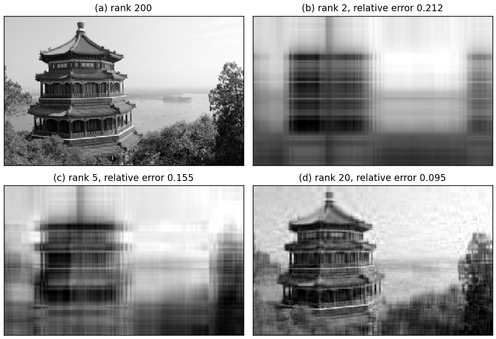
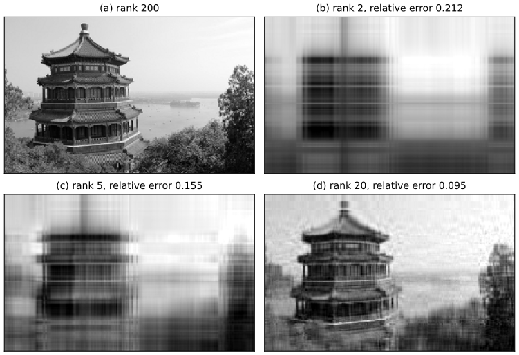
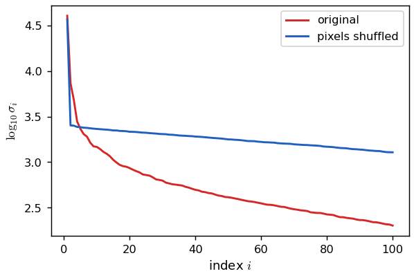
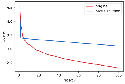
7.6 Other matrix decompositions *
7.6.1 LU factorization
pp. 264–265, (7.202), (7.203) A square matrix is factorised as \(\A=\mathbf L\U\), lower times upper triangular (7.202). If \(a_{11}=0\) this is impossible without reordering (\(a_{11}=l_{11}u_{11}\) would make \(\mathbf L\) or \(\U\) singular), so rows are swapped as the elimination proceeds: \(\mathbf P\A=\mathbf L\U\) with a permutation matrix \(\mathbf P\) (7.203), partial pivoting.
Filling the gap 7.28: Gaussian elimination is an LU factorisation, and why one pivots pp. 264–265
Derivation
Elimination as a product. Step \(k\) subtracts multiples \(\ell_{ik}=a^{(k)}_{ik}/a^{(k)}_{kk}\) of row \(k\) from the rows \(i>k\), i.e. multiplies by \(\mathbf M_k=\I-\bm\ell_k\mathbf e_k^\T\), where \(\bm\ell_k\) holds the multipliers in places \(k+1,\dots,n\). After \(n-1\) steps \(\mathbf M_{n-1}\cdots\mathbf M_1\A=\U\) is upper triangular. Each \(\mathbf M_k^{-1}=\I+\bm\ell_k\mathbf e_k^\T\), and because \(\mathbf e_j^\T\bm\ell_k=0\) for \(j\le k\), the product \(\mathbf M_1^{-1}\cdots\mathbf M_{n-1}^{-1}\)\({}=\I+\sum_k\bm\ell_k\mathbf e_k^\T\)\({}=\mathbf L\) is unit lower triangular with the multipliers below the diagonal. So \(\A=\mathbf L\U\), provided no pivot \(a^{(k)}_{kk}\) is zero; this holds iff the leading principal submatrices \(\A_{1:k,1:k}\), \(k\lt n\), are invertible (their determinants are the products of the first \(k\) pivots).
With pivoting it always works. At step \(k\), swap into position \(k\) the row with the largest \(|a^{(k)}_{ik}|\), \(i\ge k\). If that column is all zero below the diagonal, skip the step (then \(\A\) is singular and \(\U\) has a zero pivot). The swaps can be moved to the front, giving \(\mathbf P\A=\mathbf L\U\) for every square \(\A\), with \(|\ell_{ik}|\le1\).
Why pivot even when not forced. For \(\A=\begin{pmatrix}\epsilon&1\\1&1\end{pmatrix}\) with tiny \(\epsilon\), elimination without pivoting has multiplier \(1/\epsilon\) and \(u_{22}=1-1/\epsilon\); in floating point the information in \(a_{22}=1\) is lost and the computed solution can be wrong in every digit, although \(\kappa(\A)\approx2.6\). With pivoting the multiplier is \(\epsilon\) and the result is accurate. Cost: \(\tfrac23n^3\) flops for the factorisation, \(2n^2\) per right-hand side afterwards. The routine lu_partial_pivot implements this and agrees with SciPy's LU to rounding error; it solves the book's system (7.210)–(7.214) as \(\x=(1,-2,-2)\). ∎
7.6.2 QR decomposition
p. 265, (7.204)–(7.208) For \(\A\in\R^{m\times n}\) with independent columns (\(m\ge n\)) we want orthonormal \(\mathbf q_1,\mathbf q_2,\dots\) spanning the nested subspaces \(\Span\{\mathbf a_1\}\), \(\Span\{\mathbf a_1,\mathbf a_2\}\), ...: \(\mathbf a_j=\sum_{i\le j}r_{ij}\mathbf q_i\) (7.204)–(7.207), i.e.
\[ \A=\hat{\mathbf Q}\hat{\mathbf R}, \tag{7.208} \]with \(\hat{\mathbf Q}\in\R^{m\times n}\) orthonormal columns and \(\hat{\mathbf R}\in\R^{n\times n}\) upper triangular: the reduced (economy) QR. The full QR appends \(m-n\) orthonormal columns to \(\hat{\mathbf Q}\) and zero rows to \(\hat{\mathbf R}\). Figure 7.11 shows the shapes (a schematic, not reproduced).
Filling the gap 7.29: Gram–Schmidt constructs the QR factorisation; uniqueness p. 265
Derivation
Construction. Set \(r_{11}=\|\mathbf a_1\|\), \(\mathbf q_1=\mathbf a_1/r_{11}\). For \(j=2,\dots,n\): \(r_{ij}=\mathbf q_i^\T\mathbf a_j\) for \(i\lt j\), \(\mathbf w_j\)\({}=\mathbf a_j-\sum_{i\lt j}r_{ij}\mathbf q_i\), \(r_{jj}=\|\mathbf w_j\|\), \(\mathbf q_j=\mathbf w_j/r_{jj}\). By induction \(\Span\{\mathbf q_1,\dots,\mathbf q_j\}\)\({}=\Span\{\mathbf a_1,\dots,\mathbf a_j\}\); \(\mathbf w_j\) is orthogonal to the earlier \(\mathbf q_i\) by construction, and \(\mathbf w_j\ne\mathbf 0\) because \(\mathbf a_j\notin\Span\{\mathbf a_1,\dots,\mathbf a_{j-1}\}\). Rearranging the definition of \(\mathbf w_j\) gives \(\mathbf a_j=\sum_{i\le j}r_{ij}\mathbf q_i\), which is (7.208) with \(r_{jj}>0\).
Uniqueness. If \(\A\)\({}=\mathbf Q_1\mathbf R_1\)\({}=\mathbf Q_2\mathbf R_2\) with positive diagonals, then \(\A^\T\A\)\({}=\mathbf R_1^\T\mathbf R_1\)\({}=\mathbf R_2^\T\mathbf R_2\) are two Cholesky factorisations of a positive definite matrix, which is unique (Gap 7.30), so \(\mathbf R_1=\mathbf R_2\) and \(\mathbf Q_1=\mathbf Q_2\).
Numerics. Classical Gram–Schmidt loses orthogonality in floating point when the columns are nearly dependent. The modified version (subtract each projection from the running \(\mathbf w_j\), as gram_schmidt_qr does) is better, and Householder reflections, used by LAPACK and by numpy.linalg.qr, give \(\hat{\mathbf Q}\) orthogonal to machine precision. QR is the standard way to solve least squares (Gap 7.32). ∎
7.6.3 Cholesky decomposition
p. 266, (7.209) Every symmetric positive definite \(\A\) factorises as \(\A\)\({}=\mathbf R^\T\mathbf R\)\({}=\mathbf L\mathbf L^\T\) with triangular factors with positive diagonal; the cost is \(\tfrac13n^3\) flops (\(O(V^3)\) in the book's notation). (The book also calls this "matrix square root"; note that \(\mathbf L\) is not a square root in the sense \(\mathbf L^2=\A\) of Section 7.2.3.) To sample \(\y\sim\N(\bm\mu,\Sig)\) with \(\Sig=\mathbf L\mathbf L^\T\), draw \(\x\sim\N(\mathbf 0,\I)\) and set \(\y=\mathbf L\x+\bm\mu\), since
\[ \Cov[\y]=\mathbf L\Cov[\x]\mathbf L^\T=\mathbf L\I\mathbf L^\T=\Sig. \tag{7.209} \]Filling the gap 7.30: existence and uniqueness of the Cholesky factor p. 266
Derivation
Induction on \(n\); \(n=1\): \(L_{11}=\sqrt{a_{11}}\), with \(a_{11}>0\). For \(n>1\) write \(\A=\begin{pmatrix}a&\b^\T\\ \b&\mathbf C\end{pmatrix}\). Positive definiteness gives \(a=\mathbf e_1^\T\A\mathbf e_1>0\), and the Schur complement \(\mathbf C-\b\b^\T/a\) is positive definite (Gap 7.16). By induction it equals \(\mathbf L'\mathbf L'^\T\) with a unique lower-triangular \(\mathbf L'\) with positive diagonal, and then
\[ \A=\begin{pmatrix}\sqrt a&\mathbf 0\\ \b/\sqrt a&\mathbf L'\end{pmatrix}\begin{pmatrix}\sqrt a&\b^\T/\sqrt a\\ \mathbf 0&\mathbf L'^\T\end{pmatrix}. \]Uniqueness: comparing the first columns of \(\A=\mathbf L\mathbf L^\T\) forces \(L_{11}=\sqrt a\) (positive root) and the rest of the first column to be \(\b/\sqrt a\); the remaining block is the factor of the Schur complement, unique by induction. Conversely, if \(\A=\mathbf L\mathbf L^\T\) with \(\mathbf L\) invertible, \(\x^\T\A\x=\|\mathbf L^\T\x\|^2>0\): a symmetric matrix is positive definite iff it has a Cholesky factor, and the algorithm (cholesky) doubles as the cheapest test of positive definiteness: it fails exactly when a pivot \(a-\dots\) is not positive. The product of the squared pivots is \(\det\A\), which gives (7.44) and Sylvester's criterion. ∎
7.7 Solving systems of linear equations *
pp. 266–267, (7.210)–(7.214) The system \(3x_1+2x_2-x_3=1\), \(2x_1-2x_2+4x_3=-2\), \(-x_1+\frac12x_2-x_3=0\) is \(\A\x=\b\) with \(\A=\begin{pmatrix}3&2&-1\\2&-2&4\\-1&\frac12&-1\end{pmatrix}\), \(\b=(1,-2,0)\) (7.213), (7.214), and its solution is \(\x=(1,-2,-2)\) (confirmed with the LU code). With \(m\) equations and \(n\) unknowns: if \(m=n\) and \(\A\) has full rank there is one solution; if \(m\lt n\) (underdetermined) infinitely many or none; if \(m>n\) (overdetermined) generally none, and one asks for the best compromise. Figure 7.12 shows the three cases with \(n=2\).
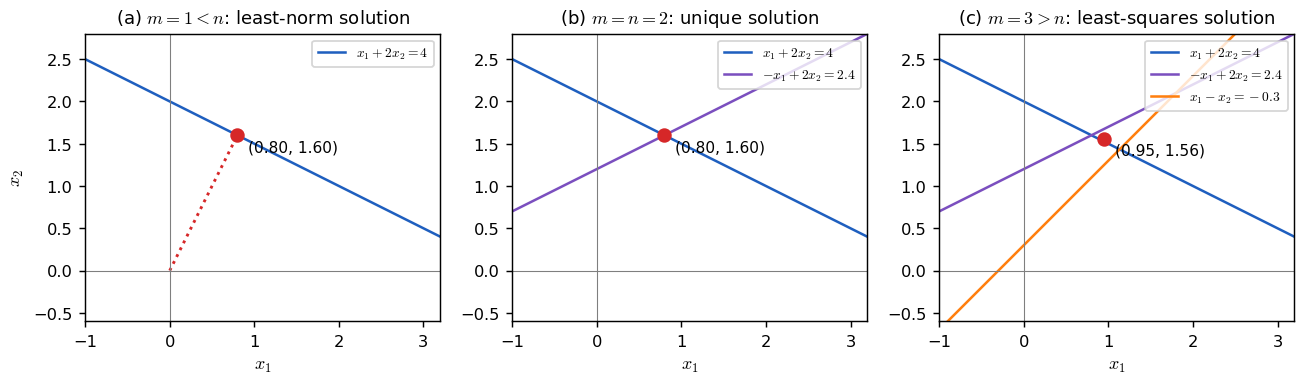
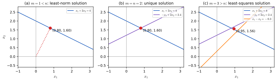
7.7.1 Solving square systems
p. 267, (7.215)–(7.220) With \(\A=\mathbf L\U\) (or \(\mathbf P\A=\mathbf L\U\)), solve \(\mathbf L\y=\b\) (or \(\mathbf P\b\)) by forward substitution, starting from \(L_{11}y_1=b_1\) and then \(L_{21}y_1+L_{22}y_2=b_2\), and so on (7.219), (7.220), then \(\U\x=\y\) by back substitution (7.215)–(7.218). MATLAB writes this \(\x=\A\backslash\b\).
Filling the gap 7.31: triangular solves, their cost, and why not to invert p. 267
Derivation
Row \(i\) of \(\mathbf L\y=\b\) reads \(\sum_{j\le i}L_{ij}y_j=b_i\), so \(y_i=(b_i-\sum_{j\lt i}L_{ij}y_j)/L_{ii}\) is determined once \(y_1,\dots,y_{i-1}\) are known, provided \(L_{ii}\ne0\) (true for an invertible triangular matrix, whose determinant is \(\prod L_{ii}\)). Row \(i\) costs about \(2i\) flops, the whole solve \(\approx n^2\). Back substitution is the same from the bottom up. So \(\A\x=\b\) costs \(\tfrac23n^3+2n^2\) flops, and further right-hand sides only \(2n^2\). Forming \(\A^{-1}\) costs \(2n^3\) and then \(\A^{-1}\b\) is no more accurate (usually less) than the triangular solves: compute \(\A^{-1}\b\) as a solve, never as a product with an explicit inverse. The functions forward_sub, back_sub and lu_solve agree with numpy.linalg.solve to rounding error. ∎
7.7.2 Solving underconstrained systems (least norm estimation)
pp. 267–268, (7.221)–(7.228) For \(m\lt n\) and independent rows, the solutions are \(\{\x_p+\mathbf z:\mathbf z\in\nullsp\A\}\) for any particular \(\x_p\) (7.221). The one of smallest norm,
\[ \hat\x=\argmin_\x\|\x\|_2^2\ \text{ s.t. }\A\x=\b, \tag{7.222} \] \[ \x_{\rm pinv}=\A^\T(\A\A^\T)^{-1}\b, \tag{7.223} \]is found in two ways in the book, both complete: by orthogonality, \((\x-\x_{\rm pinv})^\T\x_{\rm pinv}=0\) for any other solution \(\x\), so \(\|\x\|^2\)\({}=\|\x_{\rm pinv}\|^2+\|\x-\x_{\rm pinv}\|^2\) (7.224), (7.225); and by Lagrange multipliers, \(2\x+\A^\T\bm\lambda=\mathbf 0\), \(\A\x=\b\), giving \(\bm\lambda=-2(\A\A^\T)^{-1}\b\) (7.226)–(7.228). Two additions: the rows need to be independent for \(\A\A^\T\) to be invertible; if they are not, the system may have no solution, and when it has one, the least-norm solution is \(\A^\dagger\b\) (Gap 7.26). And \(\x_{\rm pinv}\) lies in the row space \(\range(\A^\T)\), the orthogonal complement of the null space (Gap 7.2), which is the geometric content of (7.224). (The book skips equation numbers (7.229)–(7.232) on purpose, after removing erroneous material from an earlier version.)
7.7.3 Solving overconstrained systems (least squares estimation)
pp. 268–269, (7.233)–(7.238) For \(m>n\) minimise
\[ f(\x)=\tfrac12\|\A\x-\b\|_2^2, \tag{7.233} \] \[ \mathbf g(\x)=\A^\T\A\x-\A^\T\b,\qquad \A^\T\A\x=\A^\T\b,\qquad \hat\x=(\A^\T\A)^{-1}\A^\T\b, \tag{7.234--7.236} \]the gradient, the normal equations and the ordinary least squares solution. The Hessian is \(\mathbf H=\A^\T\A\) (7.237), and if \(\A\) has full column rank, \(\v^\T\A^\T\A\v=\|\A\v\|^2>0\) for every \(\v\ne\mathbf 0\) (7.238; the book writes "for any \(\v>0\)", which should be \(\v\ne\mathbf 0\)), so the minimum is unique.
Filling the gap 7.32: why the stationary point is the global minimum, and how to solve least squares accurately pp. 268–269
Derivation
Global minimum without calculus. For any \(\x\), \(\A\x-\b=\A(\x-\hat\x)+(\A\hat\x-\b)\), and the second term is orthogonal to \(\range\A\) by the normal equations, so \(\|\A\x-\b\|^2\)\({}=\|\A(\x-\hat\x)\|^2+\|\A\hat\x-\b\|^2\)\({}\ge\|\A\hat\x-\b\|^2\), with equality iff \(\A(\x-\hat\x)=\mathbf 0\), iff \(\x=\hat\x\) when the columns are independent. (The calculus route: \(f\) is a convex quadratic with positive definite Hessian, so its unique stationary point is the global minimum.)
The normal equations square the condition number. \(\kappa(\A^\T\A)\)\({}=\sigma_1^2/\sigma_n^2\)\({}=\kappa(\A)^2\), so solving (7.235) by Cholesky loses about \(2\log_{10}\kappa(\A)\) digits. With \(\A=\hat{\mathbf Q}\hat{\mathbf R}\), the normal equations become \(\hat{\mathbf R}^\T\hat{\mathbf R}\x\)\({}=\hat{\mathbf R}^\T\hat{\mathbf Q}^\T\b\), i.e. \(\hat{\mathbf R}\x=\hat{\mathbf Q}^\T\b\), a triangular system with \(\kappa(\hat{\mathbf R})=\kappa(\A)\); Householder QR solves least squares with error of order \(\epsilon\kappa(\A)\) when the residual is small (and \(\epsilon\kappa^2\times\)residual otherwise, a limit no method beats; Higham, 2002, Chapter 20). The SVD route \(\x=\A^\dagger\b\) is as accurate and also handles rank deficiency. Figure 7.S4 shows the difference on polynomial fits: with \(\kappa(\A)\approx10^8\) the normal equations give a relative error of about 1, QR about \(10^{-8}\). ∎
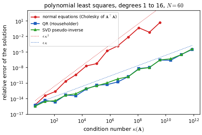
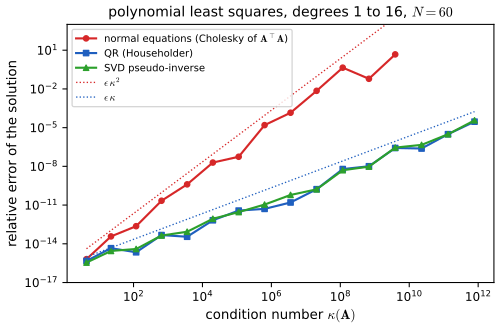
See also (companion courses): least squares and its QR computation in Section 3.2 and Section 3.9 of Statistical Learning: Theory and Methods; the geometry in Section 3.1.2 of Bayesian and Probabilistic Machine Learning. Chapter 11 of this book returns to linear regression.
7.8 Matrix calculus
7.8.1 Derivatives
pp. 269–270, (7.239)–(7.241) The derivative \(f'(x)=\lim_{h\to0}(f(x+h)-f(x))/h\) (7.239) gives the linear approximation \(f(x+h)\approx f(x)+f'(x)h\) (7.240). Finite differences replace the limit by a small \(h\):
\[ f'(x)\approx\underbrace{\frac{f(x+h)-f(x)}h}_{\text{forward}}\approx\underbrace{\frac{f(x+h/2)-f(x-h/2)}h}_{\text{central}}\approx\underbrace{\frac{f(x)-f(x-h)}h}_{\text{backward}}. \tag{7.241} \]The book says that smaller \(h\) is better "although if \(h\) is too small, there can be errors due to numerical cancellation". The trade-off can be quantified.
Filling the gap 7.33: truncation against rounding, and the best step p. 270
Derivation
Truncation error (Taylor's theorem, \(f\) smooth). Forward: \(f(x+h)=f(x)+hf'(x)+\tfrac{h^2}2f''(\xi)\), so the error is \(\tfrac h2f''(\xi)=O(h)\). Central: the even terms cancel, \(f(x\pm h/2)\)\({}=f\pm\tfrac h2f'+\tfrac{h^2}8f''\pm\tfrac{h^3}{48}f'''+\dots\), so the error is \(\tfrac{h^2}{24}f'''+O(h^4)=O(h^2)\).
Rounding error. Each evaluation of \(f\) carries a relative error of about the unit roundoff \(\epsilon\approx1.1\times10^{-16}\), so the numerator has an absolute error of up to about \(2\epsilon|f(x)|\), divided by \(h\): \(O(\epsilon/h)\), growing as \(h\) shrinks.
Balancing. Forward: \(\tfrac h2|f''|+\tfrac{2\epsilon|f|}h\) is minimal at \(h^*\)\({}=2\sqrt{\epsilon|f|/|f''|}\sim\sqrt\epsilon\)\({}\approx10^{-8}\), with error \(\sim\sqrt\epsilon\approx10^{-8}\): half the digits are lost. Central: \(\tfrac{h^2}{24}|f'''|+\tfrac{2\epsilon|f|}h\) is minimal at \(h^*\sim\epsilon^{1/3}\approx5\times10^{-6}\), with error \(\sim\epsilon^{2/3}\approx10^{-11}\). Figure 7.S3 shows both V-shaped curves for \(f=\exp\) at \(x=1\). Automatic differentiation (Section 13.3) has no truncation error at all. ∎
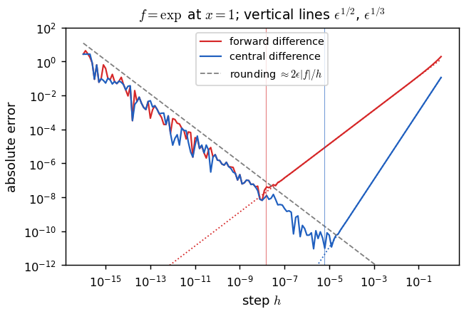
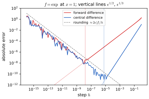
Notation: Lagrange writes \(f'\), \(f''\), \(f^{(n)}\); Leibniz writes \(\frac{\d y}{\d x}\) and \(\frac{\d f}{\d x}\big|_{x=a}\).
7.8.2–7.8.4 Gradients, directional derivatives and total derivatives
pp. 270–271, (7.242)–(7.248) For \(f:\R^n\to\R\) the partial derivatives are \(\partial f/\partial x_i\)\({}=\lim_{h\to0}(f(\x+h\mathbf e_i)-f(\x))/h\) (7.242) and the gradient is the vector \(\nabla f\)\({}=(\partial f/\partial x_1,\dots,\partial f/\partial x_n)\) (7.243), (7.244). The directional derivative along \(\v\) is
\[ D_\v f(\x)=\lim_{h\to0}\frac{f(\x+h\v)-f(\x)}h,\qquad D_\v f(\x)=\nabla f(\x)\cdot\v. \tag{7.245, 7.246} \]It needs two function calls numerically, against \(n+1\) (or \(2n\)) for the gradient. For \(f(t,x(t),y(t))\) the total derivative is \(\frac{\d f}{\d t}\)\({}=\frac{\partial f}{\partial t}+\frac{\partial f}{\partial x}\frac{\d x}{\d t}+\frac{\partial f}{\partial y}\frac{\d y}{\d t}\) (7.247), the chain rule; multiplied by \(\d t\) it is the total differential (7.248).
7.8.5 Jacobian
pp. 271–272, (7.249)–(7.254) For \(\mathbf f:\R^n\to\R^m\) the Jacobian is the \(m\times n\) matrix \(\mathbf J_{\mathbf f}(\x)\)\({}=\partial\mathbf f/\partial\x^\T\) whose rows are the gradients \(\nabla f_i^\T\) (7.249) (numerator layout). The Jacobian–vector product \(\mathbf J\v\) (7.250) and the vector–Jacobian product \(\u^\T\mathbf J\) (7.251) are the building blocks of forward- and reverse-mode automatic differentiation; the book says the JVP is more efficient when \(m\ge n\) and the VJP when \(m\le n\). For a composition \(\mathbf h=\mathbf g\circ\mathbf f\), the chain rule is
\[ \mathbf J_{\mathbf h}(\x)=\mathbf J_{\mathbf g}(\mathbf f(\x))\,\mathbf J_{\mathbf f}(\x), \tag{7.252} \]with the scalar-input example (7.253), (7.254).
Filling the gap 7.34: when (7.246) holds, the chain rule (7.252), and the cost of JVPs and VJPs pp. 271–272
Derivation
Differentiability is needed for (7.246). If \(f\) is (Fréchet) differentiable at \(\x\), \(f(\x+h\v)=f(\x)+h\nabla f(\x)^\T\v+o(h)\), and dividing by \(h\) gives (7.246). Existence of the partial derivatives is not enough: \(f(x,y)=x^2y/(x^2+y^2)\), \(f(0,0)=0\), has \(\nabla f(\mathbf 0)=\mathbf 0\) but \(D_\v f(\mathbf 0)=v_1^2v_2/(v_1^2+v_2^2)\ne0\) for \(\v=(1,1)\); this \(f\) is not differentiable at the origin. Continuous partial derivatives are a sufficient condition.
Chain rule. Write \(\mathbf f(\x+\bm\delta)\)\({}=\mathbf f(\x)+\mathbf J_{\mathbf f}\bm\delta+o(\|\bm\delta\|)\) and \(\mathbf g(\y+\bm\eta)\)\({}=\mathbf g(\y)+\mathbf J_{\mathbf g}\bm\eta+o(\|\bm\eta\|)\). With \(\y=\mathbf f(\x)\) and \(\bm\eta\)\({}=\mathbf J_{\mathbf f}\bm\delta+o(\|\bm\delta\|)\)\({}=O(\|\bm\delta\|)\), \(\mathbf h(\x+\bm\delta)\)\({}=\mathbf h(\x)+\mathbf J_{\mathbf g}\mathbf J_{\mathbf f}\bm\delta+o(\|\bm\delta\|)\), which identifies \(\mathbf J_{\mathbf h}\). Entry by entry this is (7.253).
Costs. For a chain \(\mathbf h\)\({}=\mathbf f_L\circ\dots\circ\mathbf f_1\), \(\mathbf J_{\mathbf h}\)\({}=\mathbf J_L\cdots\mathbf J_1\). A JVP evaluates \(\mathbf J_L(\cdots(\mathbf J_1\v))\) from right to left alongside the forward computation, at a cost of a small multiple of evaluating \(\mathbf h\); a VJP evaluates \(((\u^\T\mathbf J_L)\cdots)\mathbf J_1\) from left to right after a forward pass. The full \(m\times n\) Jacobian needs \(n\) JVPs (one per input direction) or \(m\) VJPs (one per output), hence forward mode when \(n\le m\) and reverse mode when \(m\le n\), as the book says. For a scalar loss of many parameters (\(m=1\)) one VJP gives the whole gradient: that is backpropagation. ∎
See also (companion course): forward- and reverse-mode automatic differentiation and numerical differentiation in Foundations of Deep Learning.
7.8.6 Hessian
p. 272, (7.255) For twice-differentiable \(f:\R^n\to\R\), the Hessian \(\mathbf H_f=\nabla^2f\) has entries \(\partial^2f/\partial x_i\partial x_j\) (7.255); it is the Jacobian of the gradient. The book calls it symmetric.
Filling the gap 7.35: symmetry of the Hessian p. 272
Derivation
Schwarz (Clairaut). If the second partials of \(f\) are continuous near \(\x\), then \(\partial_i\partial_jf=\partial_j\partial_if\) at \(\x\). Proof: let
\[ \Delta(h)=f(\x+h\mathbf e_i+h\mathbf e_j)-f(\x+h\mathbf e_i)-f(\x+h\mathbf e_j)+f(\x). \]Applying the mean value theorem twice, first in the \(\mathbf e_i\) direction and then in \(\mathbf e_j\), gives \(\Delta(h)=h^2\partial_j\partial_if(\bm\xi)\) for some \(\bm\xi\) in the square of side \(h\); in the other order, \(\Delta(h)=h^2\partial_i\partial_jf(\bm\xi')\). Divide by \(h^2\) and let \(h\to0\); continuity gives equality.
Without continuity it can fail. \(f(x,y)=xy(x^2-y^2)/(x^2+y^2)\), \(f(0,0)=0\), has \(\partial_x\partial_yf(0,0)=1\) but \(\partial_y\partial_xf(0,0)=-1\). For the smooth losses of machine learning the Hessian is symmetric, and at a minimum it is positive semidefinite (Chapter 8). ∎
7.8.7 Gradients of commonly used functions
pp. 272–274, (7.256)–(7.273) The scalar rules (7.256)–(7.261) end with the chain rule \(\frac{\d}{\d x}f(u(x))\)\({}=\frac{\d u}{\d x}\frac{\d f}{\d u}\). For \(f:\R^n\to\R\):
\[ \frac{\partial(\mathbf a^\T\x)}{\partial\x}=\mathbf a,\qquad \frac{\partial(\b^\T\A\x)}{\partial\x}=\A^\T\b,\qquad \frac{\partial(\x^\T\A\x)}{\partial\x}=(\A+\A^\T)\x. \tag{7.262--7.264} \]For \(f:\R^{m\times n}\to\R\), with \(\partial f/\partial\X\) the matrix of partial derivatives \(\partial f/\partial x_{ij}\) (7.265):
\[ \frac{\partial}{\partial\X}(\mathbf a^\T\X\b)=\mathbf a\b^\T,\qquad \frac{\partial}{\partial\X}(\mathbf a^\T\X^\T\b)=\b\mathbf a^\T, \tag{7.266, 7.267} \] \[ \frac{\partial}{\partial\X}\tr(\A\X\B)=\A^\T\B^\T,\quad \frac{\partial}{\partial\X}\tr(\X^\T\A)=\A,\quad \frac{\partial}{\partial\X}\tr(\X^{-1}\A)=-\X^{-\T}\A^\T\X^{-\T},\quad \frac{\partial}{\partial\X}\tr(\X^\T\A\X)=(\A+\A^\T)\X, \tag{7.268--7.271} \] \[ \frac{\partial}{\partial\X}\det(\A\X\B)=\det(\A\X\B)\,\X^{-\T},\qquad \frac{\partial}{\partial\X}\log\det(\X)=\X^{-\T}. \tag{7.272, 7.273} \]The book lists these "without proof"; (7.272) needs \(\A\), \(\X\), \(\B\) square and invertible, and (7.273) needs \(\det\X>0\) (in general the identity holds for \(\log|\det\X|\)).
Filling the gap 7.36: all the gradient identities from one rule pp. 273–274
Derivation
The rule. If, for every perturbation \(\d\X\), the first-order change of \(f\) is \(\d f\)\({}=\tr(\mathbf G^\T\d\X)\)\({}=\sum_{ij}G_{ij}\,\d X_{ij}\), then \(\partial f/\partial\X=\mathbf G\). For vectors this reads \(\d f\)\({}=\mathbf g^\T\d\x\)\({}\Rightarrow\nabla f\)\({}=\mathbf g\).
Vectors. \(\d(\mathbf a^\T\x)=\mathbf a^\T\d\x\) (7.262). \(\d(\b^\T\A\x)=(\A^\T\b)^\T\d\x\) (7.263). \(\d(\x^\T\A\x)\)\({}=\d\x^\T\A\x+\x^\T\A\d\x\)\({}=\x^\T(\A^\T+\A)\d\x\) (7.264); for symmetric \(\A\) this is \(2\A\x\).
Bilinear forms. \(\d(\mathbf a^\T\X\b)\)\({}=\mathbf a^\T\d\X\b\)\({}=\tr(\b\mathbf a^\T\d\X)\), so \(\mathbf G^\T=\b\mathbf a^\T\), \(\mathbf G=\mathbf a\b^\T\) (7.266). Transposing the scalar, \(\mathbf a^\T\X^\T\b=\b^\T\X\mathbf a\), gives (7.267).
Traces. \(\d\tr(\A\X\B)=\tr(\B\A\,\d\X)\), \(\mathbf G=(\B\A)^\T=\A^\T\B^\T\) (7.268). \(\tr(\X^\T\A)=\tr(\A^\T\X)\), \(\mathbf G=\A\) (7.269). Differentiating \(\X\X^{-1}=\I\) gives \(\d(\X^{-1})=-\X^{-1}\d\X\,\X^{-1}\), so \(\d\tr(\X^{-1}\A)=-\tr(\X^{-1}\A\X^{-1}\d\X)\) and \(\mathbf G\)\({}=-(\X^{-1}\A\X^{-1})^\T\)\({}=-\X^{-\T}\A^\T\X^{-\T}\) (7.270). \(\d\tr(\X^\T\A\X)\)\({}=\tr(\d\X^\T\A\X)+\tr(\X^\T\A\d\X)\)\({}=\tr(\X^\T(\A^\T+\A)\d\X)\), \(\mathbf G=(\A+\A^\T)\X\) (7.271).
Determinants. Jacobi's formula \(\d\det\X=\det\X\,\tr(\X^{-1}\d\X)\) follows from \(\det(\X+\d\X)=\det\X\det(\I+\X^{-1}\d\X)\) and \(\det(\I+\mathbf E)\)\({}=1+\tr\mathbf E+O(\|\mathbf E\|^2)\) (expand the Leibniz sum: only the identity permutation contributes first-order terms). Then \(\d\log\det\X=\tr(\X^{-1}\d\X)\), \(\mathbf G=\X^{-\T}\) (7.273), valid wherever \(\det\X>0\) (and for \(\log|\det\X|\) wherever \(\det\X\ne0\)). For (7.272), \(\d\det(\A\X\B)\)\({}=\det(\A\X\B)\tr((\A\X\B)^{-1}\A\,\d\X\,\B)\)\({}=\det(\A\X\B)\tr(\B(\A\X\B)^{-1}\A\,\d\X)\); when all three matrices are square and invertible, \(\B(\A\X\B)^{-1}\A=\X^{-1}\), giving \(\det(\A\X\B)\X^{-\T}\). For rectangular \(\A\), \(\B\) (with \(\A\X\B\) square and invertible) the general answer is \(\det(\A\X\B)\,\A^\T(\A\X\B)^{-\T}\B^\T\).
Each identity was confirmed against central finite differences on random matrices (relative agreement about \(10^{-9}\), the accuracy of the differences). ∎
See also (companion courses): matrix derivatives by differentials (with the symmetric-matrix subtlety for covariance parameters), and Appendix A.3 of Foundations of Deep Learning.
Notes on the book: points that need a correction or a qualification
- Truncated SVD error (7.201). The text gives \(\|\A-\hat\A_K\|_F=\sum_{k>K}\sigma_k\). The correct value is \(\big(\sum_{k>K}\sigma_k^2\big)^{1/2}\); the sum of the \(\sigma_k\) is the nuclear norm of the residual. For the image of Figure 7.9 at \(K=20\) the relative errors are 0.095 (correct, and what one measures) against 0.976 (Result 7.5).
- Rank and eigenvalues (Section 7.4.1). "The rank of \(\A\) is equal to the number of non-zero eigenvalues" fails for \(\begin{pmatrix}0&1\\0&0\end{pmatrix}\) (rank 1, both eigenvalues 0). It holds for diagonalisable, in particular symmetric, matrices; the rank is always the number of non-zero singular values (Gap 7.18).
- Diagonal dominance (7.58). Strict diagonal dominance implies positive definiteness only if the diagonal entries are positive; \(\begin{pmatrix}-2&1\\1&-2\end{pmatrix}\) is diagonally dominant and negative definite (Gap 7.10).
- Theorem 7.3.1. "Assume \(\mathbf E\) and \(\mathbf H\) are invertible" must be supplemented by "\(\mathbf M\) is invertible" (equivalently, the Schur complement is): \(\mathbf M=\begin{pmatrix}1&1\\1&1\end{pmatrix}\) (Gap 7.16).
- Double centring (7.89), (7.90). The last term of (7.89) is a scalar added to a matrix; as a matrix it is \(\frac1{N^2}(\mathbf 1^\T\mathbf K\mathbf 1)\mathbf J\). (7.90) is missing the transpose in \((\x_i-\bar\x)^\T(\x_j-\bar\x)\) (Gap 7.12).
- Least squares (7.238). "For any \(\v>0\)" should read "for any \(\v\ne\mathbf 0\)".
- Figure 7.7(b). The axis ranges of the "standardized" panel (about \(\pm0.1\) and \(-1\) to \(1.5\)) are incompatible with unit variance in both columns; they look like division by a single pooled standard deviation rather than by each column's own, as (7.82) prescribes.
- Figure 7.6. The semi-axes are labelled \(\lambda_i^{1/2}\), which is right for the eigenvalues of \(\Sig\), while the text has \(\lambda_i\) the eigenvalues of \(\A=\Sig^{-1}\) and semi-axes \(\lambda_i^{-1/2}\) (Section 7.4.4).
- Figure 7.4 caption. The range of \(\A\) is a subspace of the output space \(\R^m\), not of the input domain; and the row space is the orthogonal complement of the null space (Gap 7.2).
- Notation (7.26). The Schatten \(p\)-norm is written \(\|\A\|_p\), the symbol already used for the induced \(p\)-norm (7.22); the two differ (the Schatten 2-norm is the Frobenius norm, the induced 2-norm is \(\sigma_1\)).
- Power method (Section 7.4.6). The start vector need not lie in the range of \(\A\); what is needed is \(\u_1^\T\v_0\ne0\) and a strict gap in magnitude, \(|\lambda_1|>|\lambda_2|\) (Gap 7.22).
- Determinant gradients (7.272), (7.273). (7.272) assumes \(\A\), \(\X\), \(\B\) square and invertible; (7.273) assumes \(\det\X>0\) (Gap 7.36).
- Terminology. The Cholesky factor is called a "matrix square root" (Section 7.6.3) although Section 7.2.3 defines \(\sqrt{\mathbf M}\) by \(\A^2=\mathbf M\); and Gram–Schmidt does not "make any square matrix orthogonal" but orthonormalises independent columns (Section 7.1.5.4).
7.9 Exercises
Both exercises of Chapter 7 (Murphy, 2022, p. 274), restated in my own words, with complete solutions (hidden). The computational parts were also checked numerically.
Exercise 7.1 (orthogonal matrices). (a) The rotation of \(\R^3\) by an angle \(\alpha\) about the \(z\) axis is \(\mathbf R(\alpha)\) of (7.274) (the same matrix as (7.60)). Prove that \(\mathbf R(\alpha)^\T\mathbf R(\alpha)=\I\) for every \(\alpha\). (b) Find the unit eigenvector of \(\mathbf R(\alpha)\) with eigenvalue 1; the answer should not depend on \(\alpha\). Hint: think about what a rotation leaves fixed.
Solution
(a) Write \(c=\cos\alpha\), \(s=\sin\alpha\). Then
\[ \mathbf R^\T\mathbf R=\begin{pmatrix}c&s&0\\-s&c&0\\0&0&1\end{pmatrix}\begin{pmatrix}c&-s&0\\s&c&0\\0&0&1\end{pmatrix}=\begin{pmatrix}c^2+s^2&-cs+sc&0\\-sc+cs&s^2+c^2&0\\0&0&1\end{pmatrix}=\I, \]using \(c^2+s^2=1\). (Since \(\mathbf R\) is square, \(\mathbf R\mathbf R^\T=\I\) follows, Gap 7.11; also \(\det\mathbf R=c^2+s^2=1\), so it is a rotation, not a reflection.)
(b) Points on the axis of rotation do not move: \(\mathbf R\mathbf e_3=\mathbf e_3\), so \(\v=(0,0,1)\) (or \(-\v\)) is a unit eigenvector with eigenvalue 1. It is the only one (up to sign) when \(\alpha\notin2\pi\mathbb Z\): the characteristic polynomial factorises as \(\det(\lambda\I-\mathbf R)\)\({}=(\lambda-1)(\lambda^2-2c\lambda+1)\), whose quadratic factor has roots \(e^{\pm i\alpha}\); these equal 1 only if \(\alpha\in2\pi\mathbb Z\). So for \(\alpha\notin2\pi\mathbb Z\) the eigenvalue 1 is simple, and its eigenspace is the line through \(\mathbf e_3\). (For \(\alpha=\pi\) the other eigenvalue is \(-1\), double; for \(\alpha\in2\pi\mathbb Z\), \(\mathbf R=\I\) and every vector is an eigenvector, the one case where "the only eigenvector" fails.) Numerically, for \(\alpha=0.7\),
numpy.linalg.eigreturns the eigenvalues \(e^{\pm0.7i}\) and 1, with eigenvector \((0,0,1)\) for the latter.Exercise 7.2 (eigenvectors by hand). Find the eigenvalues and eigenvectors of \(\A=\begin{pmatrix}2&0\\0&3\end{pmatrix}\) (7.275) by hand, and check with Python.
Solution
The characteristic equation (7.151) is \(\det(\lambda\I-\A)=(\lambda-2)(\lambda-3)=0\), so \(\lambda_1=3\), \(\lambda_2=2\) (sorted by size). For \(\lambda=3\), \((3\I-\A)\u=(u_1,0)=\mathbf 0\) forces \(u_1=0\): \(\u_1=(0,1)\). For \(\lambda=2\), \((2\I-\A)\u=(0,-u_2)=\mathbf 0\) forces \(u_2=0\): \(\u_2=(1,0)\). Each up to sign; they are orthonormal, as the spectral theorem promises, and \(\tr\A=5=3+2\), \(\det\A=6=3\cdot2\). A diagonal matrix has the standard basis vectors as eigenvectors and its diagonal entries as eigenvalues. In Python,
numpy.linalg.eigh(np.diag([2., 3.]))returns the eigenvalues \((2,3)\) in increasing order with the identity as eigenvector matrix.
Demonstrations for this chapter
Each demonstration runs in the browser and links back to these notes. The ▶ Demo boxes above open them already set to the case under discussion.
| Demonstration | What you can see | Sections and results |
|---|---|---|
| Eigenvectors, quadratic forms and the power method | A symmetric \(2\times2\) matrix set by its eigenvalues and eigenvector; its level sets, the power-method iterates, the angle error against the bound, the Rayleigh quotient, and deflation. Presets: 1 well separated; 2 small eigengap; 3 negative dominant eigenvalue; 4 equal magnitudes; 5 deflation. | 7.4.4, 7.4.6, 7.4.7; Figures 7.6, 7.S1; Gaps 7.22, 7.23 |
| Standardising and whitening data | Height and weight data or a simulated sample; standardisation, PCA, ZCA or any rotated whitening; output covariance and mean squared displacement against the rotation. Presets: 1 standardised; 2 PCA; 3 ZCA; 4 another whitening; 5 simulated, strong correlation. | 7.4.5; Figure 7.7; Gap 7.21 |
| Truncated SVD of an image | Two images and their shuffled pixels; the rank-\(K\) approximation or residual, the singular-value spectrum, storage and the three error formulas. Presets: 1 rank 2; 2 rank 5; 3 rank 20; 4 shuffled pixels; 5 the error formula. | 7.5.2, 7.5.5; Figures 7.9, 7.10; Result 7.5 |
The Python code that produces every figure of this page is code/ch07_linear_algebra.py (see the code index). Figures 7.1–7.5, 7.8 and 7.11 are schematic diagrams (array layouts, vector addition and bases, range and null space, the matrix product, the shapes of the SVD and QR factors) and are not reproduced.
References
- Murphy, K. P. (2022). Probabilistic Machine Learning: An Introduction. MIT Press, Cambridge, MA. Chapter 7, pp. 229–274. probml.github.io/pml-book/book1.html.
- Axler, S. (2015). Linear Algebra Done Right, 3rd edition. Springer, Cham.
- Bell, A. J. and Sejnowski, T. J. (1997). The "independent components" of natural scenes are edge filters. Vision Research, 37(23), 3327–3338.
- Davis, C. (1990). Body image and weight preoccupation: a comparison between exercising and non-exercising women. Appetite, 15, 13–21. (Source of the height and weight data in the R package carData.)
- Eckart, C. and Young, G. (1936). The approximation of one matrix by another of lower rank. Psychometrika, 1(3), 211–218.
- Golub, G. H. and Van Loan, C. F. (2013). Matrix Computations, 4th edition. Johns Hopkins University Press, Baltimore.
- Higham, N. J. (2002). Accuracy and Stability of Numerical Algorithms, 2nd edition. SIAM, Philadelphia.
- Horn, R. A. and Johnson, C. R. (2013). Matrix Analysis, 2nd edition. Cambridge University Press.
- Hutchinson, M. F. (1990). A stochastic estimator of the trace of the influence matrix for Laplacian smoothing splines. Communications in Statistics: Simulation and Computation, 19(2), 433–450.
- Kessy, A., Lewin, A. and Strimmer, K. (2018). Optimal whitening and decorrelation. The American Statistician, 72(4), 309–314.
- Mirsky, L. (1960). Symmetric gauge functions and unitarily invariant norms. Quarterly Journal of Mathematics, 11(1), 50–59.
- Penrose, R. (1955). A generalized inverse for matrices. Mathematical Proceedings of the Cambridge Philosophical Society, 51(3), 406–413.
- Strang, G. (2009). Introduction to Linear Algebra, 4th edition. Wellesley-Cambridge Press, Wellesley, MA.
- Trefethen, L. N. and Bau, D. (1997). Numerical Linear Algebra. SIAM, Philadelphia.
The numerical statements in the text (the condition number of (7.49), the solution of (7.214), the projection, centring, Kronecker and einsum identities, the inversion and determinant lemmas, the spectral and SVD facts, the pseudo-inverse conditions, the Eckart–Young errors of Figure 7.9, the whitening numbers of Figure 7.7, the power-method rates, the Hutchinson variances, the finite-difference and least-squares accuracy, the gradient identities, and the solutions of the two exercises) were confirmed numerically.