The Bootstrap
How variable is a statistic? For a sample mean there is a formula; for a median, a skewness, a correlation or a ratio of means there usually is none, because the answer depends on the unknown distribution in a complicated way. The bootstrap answers the question by two substitutions: replace the unknown distribution by the empirical distribution of the data, and replace the resulting (still intractable) calculation by simulation. These notes make both substitutions precise, measure the error each one makes, prove that the bootstrap works for smooth statistics, and show three places where it or its older cousin, the jackknife, fails.
Ch. 1 Probability Ch. 2 Random variables Ch. 3 Expectation Ch. 4 Inequalities Ch. 5 Convergence Ch. 6 Models and inference Ch. 7 Estimating the CDF Ch. 8 Bootstrap Ch. 9 Parametric inference Ch. 10 Hypothesis testing Ch. 11 Bayesian inference Ch. 12 Decision theory Ch. 13 Regression Ch. 14 Multivariate models Ch. 15 Independence Ch. 16 Causal inference Ch. 17 Directed graphs Ch. 18 Undirected graphs Ch. 19 Log-linear models Ch. 20 Curve estimation Ch. 21 Orthogonal functions Ch. 22 Classification Ch. 23 Stochastic processes Ch. 24 Simulation
How to read these notes
They follow the book. Sections carry the book's numbers (8.1, 8.2, ...) and every displayed equation that appears in the book carries the book's own equation number, e.g. \((8.6)\). Numbered items keep the book's numbers (Example 8.2, Theorem 8.3); boxes the book prints without a number are lettered (Algorithm 8.A). Equations without a number are steps that the book skips.
Filling the gaps. Wherever the book says "it can be shown", quotes a fact without proof, or leaves an argument implicit, an orange Filling the gap box gives the full argument. Proofs and derivations start hidden: open one with its bar, or use the button below.
Figures and demonstrations. The book's two data figures (8.1 and 8.2) are reproduced from the data; the "real world / bootstrap world" diagram of Section 8.2 is drawn in words instead. Six supplementary figures (8.S1 to 8.S6) illustrate the gaps and the exercises. All are computed by the Python code. The ▶ Demo boxes open an interactive demonstration already set to the case being discussed.
Main reference
L. Wasserman, All of Statistics: A Concise Course in Statistical Inference, Springer (2004), Chapter 8, pages 107–118 (book website: www.stat.cmu.edu/~larry/all-of-statistics, which also hosts the nerve data and the author's errata lists). Section, equation, example and exercise numbers below refer to this book. Further reading is listed in the references.
The explanations, derivations, figures and code are my own; equations are cited by their numbers in the book.
Companion courses
The bootstrap appears, with other emphases, in four companion courses on this site:
- Applied Statistical Learning in R and Python, Section 5.2: the bootstrap standard error of any statistic (Definition 5.5, Algorithm 5.2), how large \(B\) must be (Filling the gap 5.6) and the 0.632 probability (Result 5.3); demonstrations: bootstrap of a portfolio allocation, which observations a resample contains.
- Statistical Methods for Modern Biology, Section 4.3: the empirical distribution and the nonparametric bootstrap (Definition 4.4, Algorithm 4.3), the exact bootstrap distributions of the mean and the median (Result 4.6) and why the bootstrap works for the mean (Result 4.7); demonstration: bootstrapping Darwin's Zea mays data.
- Statistical Learning: Theory and Methods, Section 7.11 (bootstrap estimates of prediction error, the .632 estimator, Result 7.14) and Section 8.2 (the bootstrap against maximum likelihood; the parametric bootstrap, Result 8.1), Section 8.4 (the bootstrap as an approximate posterior) and Section 8.7 (bagging); demonstrations: bootstrap estimates of prediction error, bootstrap and Bayesian bands.
- Bayesian and Probabilistic Machine Learning, Section 14.2: committees and bootstrap aggregation.
Where a proof there is the same, these notes give a short argument and link to it (the exact bootstrap law of the median, the bootstrap for the mean). New here: the Monte Carlo error of \(\seboot\) for any kurtosis (Filling the gap 8.2), the influence function of the skewness (8.5), a proof of Theorem 8.3 for smooth functions of means (8.7), why the three intervals have the same order of accuracy and miss on one side (8.8), the corrected percentile argument (8.9), the jackknife's exactness for the mean and its failure for the median, with the limit laws for odd and even \(n\) (8.10, 8.11), and the parametric bootstrap that rescues the maximum (8.12).
The chapter at a glance
- The idea To estimate \(\V_F(T_n)\), (1) replace \(F\) by \(\Fn\) and (2) compute \(\V_{\Fn}(T_n)\) by simulation. For the mean, step 1 alone gives \(\hs^2/n\) (Filling the gap 8.1).
- 8.1 The law of large numbers turns a simulation into an integral; its error falls like \(1/\sqrt B\), with a constant set by the kurtosis (8.2).
- 8.2 Drawing from \(\Fn\) is resampling the data with replacement (8.3). The ideal bootstrap variance \(\V_{\Fn}(T_n)\) is a function of the data only; for the median it has a closed form (8.4). The nerve-data skewness and its standard error, also by the influence function (8.5).
- 8.3 Normal, pivotal and percentile intervals (8.6); the bootstrap is consistent (Theorem 8.3, proved in 8.7); all three intervals have two-sided coverage error of the same order, but none is accurate for strongly skewed statistics (8.8). Four data examples, Figures 8.1 and 8.2.
- 8.5 The jackknife: exact for the mean, consistent for smooth statistics (8.10), inconsistent for the median (8.11). Why the percentile interval works (8.9). The parametric bootstrap, and a statistic where the nonparametric bootstrap fails (8.12).
Notation. Data \(X_1,\dots,X_n\) independent and identically distributed (iid) with cdf \(F\); \(\Fn\) is the empirical cdf, putting mass \(1/n\) on each observation. A statistic is \(T_n=g(X_1,\dots,X_n)\); when it estimates a functional \(\th=T(F)\) by plug-in we write \(\hth=T(\Fn)\). Bootstrap quantities carry a star, and \(\Ps\), \(\Es\), \(\Vs\) are probability, expectation and variance over resampling with the data held fixed. \(\hs^2=n^{-1}\sum_i(X_i-\overline X_n)^2\) (divisor \(n\)) and \(s^2=\frac n{n-1}\hs^2\). \(\Phi\) is the standard Normal cdf and \(z_{\alpha/2}=\Phi^{-1}(1-\alpha/2)\).
Prerequisites. Chapters 5 and 6: the law of large numbers, the central limit theorem and the Berry–Esseen bound (Theorem 5.11), the delta method (Theorem 5.13), confidence intervals (Definition 6.D). Chapter 7 is used freely: the empirical cdf (Definition 7.1) converges to \(F\) uniformly (Theorem 7.4), and the plug-in estimator \(T(\Fn)\) (Definition 7.7) estimates \(T(F)\).
The bootstrap idea
p. 107 Let \(T_n=g(X_1,\dots,X_n)\) be any statistic. Its variance \(\V_F(T_n)\) depends on the unknown \(F\); the subscript is a reminder of that. For the mean, \(\V_F(\overline X_n)=\sigma^2/n\) with \(\sigma^2=\int(x-\mu)^2\,\d F(x)\), a functional of \(F\). The bootstrap estimates \(\V_F(T_n)\) in two steps:
- Plug in. Estimate \(\V_F(T_n)\) by \(\V_{\Fn}(T_n)\), the variance \(T_n\) would have if the data were drawn from \(\Fn\).
- Simulate. Approximate \(\V_{\Fn}(T_n)\), which is usually impossible to compute exactly, by simulation.
For the mean, step 1 already gives a formula, \(\V_{\Fn}(\overline X_n)=\hs^2/n\) (the book's display omits the squares; see the notes on the book), so step 2 is not needed. For most statistics step 2 is the whole point.
Filling the gap 8.1: step 1 for the mean, exactly p. 107
If the data were drawn from \(\Fn\), the mean of \(n\) draws would have variance \(\hs^2/n\) with \(\hs^2=n^{-1}\sum_i(X_i-\overline X_n)^2\), the divisor-\(n\) variance.
Proof
Fix the data. A random variable \(X^*\) with cdf \(\Fn\) takes each value \(X_j\) with probability \(1/n\) (values that occur several times get the corresponding multiple). Its mean and variance are
\[ \int x\,\d\Fn(x)=\frac1n\sum_jX_j=\overline X_n,\qquad\int(x-\overline X_n)^2\,\d\Fn(x)=\frac1n\sum_j(X_j-\overline X_n)^2=\hs^2. \]If \(X_1^*,\dots,X_n^*\) are iid with cdf \(\Fn\), the variance of their mean is \(n\hs^2/n^2=\hs^2/n\) by the variance of a sum of independent terms (Result 3.9). ∎
So the bootstrap standard error of the mean is \(\hs/\sqrt n=\sqrt{(n-1)/n}\;s/\sqrt n\), slightly smaller than the textbook \(s/\sqrt n\). For the 799 nerve times: \(\hs/\sqrt n=0.0073959\) against \(s/\sqrt n=0.0074006\). The two differ by the factor \(\sqrt{(n-1)/n}\), which is negligible unless \(n\) is very small.
8.1 Simulation
p. 108 If \(Y_1,\dots,Y_B\) are iid from a distribution \(G\) and \(h\) has finite mean, the weak law of large numbers (Theorem 5.6) gives
\[ \frac1B\sum_{j=1}^Bh(Y_j)\convp\int h(y)\,\d G(y)=\E\,h(Y)\qquad(B\to\infty). \]Since we choose \(B\), a simulation can make this error as small as we like. With \(h(y)=y\) and \(h(y)=y^2\), and the identity \(B^{-1}\sum_j(Y_j-\overline Y_B)^2=B^{-1}\sum_jY_j^2-\overline Y_B^{\,2}\), the sample variance of the simulated values converges to \(\int y^2\,\d G-(\int y\,\d G)^2=\V(Y)\) (the continuous mapping part of Theorem 5.5). Two misprints in the book's displays (\(\overline Y_n\) for \(\overline Y_B\), which is in the author's errata, and \(\d F\) for \(\d G\)) are listed in the notes on the book. How large must \(B\) be?
Filling the gap 8.2: the Monte Carlo error of a simulated variance and standard error p. 108
Let \(Y_j\) be iid with variance \(\sigma^2\), fourth central moment \(\mu_4\) and kurtosis \(\kappa=\mu_4/\sigma^4\), and let \(v_B=B^{-1}\sum_{j=1}^B(Y_j-\overline Y_B)^2\). Then \(\E v_B=\frac{B-1}B\sigma^2\) and
\[ \sqrt B\,(v_B-\sigma^2)\convd\N(0,\mu_4-\sigma^4),\qquad \sqrt B\,\big(\sqrt{v_B}-\sigma\big)\convd\N\Big(0,\frac{\sigma^2(\kappa-1)}4\Big). \]So the relative Monte Carlo error of a simulated standard deviation is about \(\sqrt{(\kappa-1)/(4B)}\): for a Normal-shaped distribution (\(\kappa=3\)) that is \(1/\sqrt{2B}\), i.e. 5.0% for \(B=200\), 2.2% for \(B=1000\), 1.0% for \(B=5000\).
Proof
Write \(\mu=\E Y_j\) and expand the square around \(\mu\):
\[ v_B=\frac1B\sum_j(Y_j-\mu)^2-(\overline Y_B-\mu)^2. \]The first term has mean \(\sigma^2\) and variance \(\V((Y-\mu)^2)/B\), which is \((\mu_4-\sigma^4)/B\); the second has mean \(\V(\overline Y_B)=\sigma^2/B\), which gives \(\E v_B=\sigma^2-\sigma^2/B\). By the central limit theorem (Theorem 5.8),
\[ \sqrt B\Big(\frac1B\sum_j(Y_j-\mu)^2-\sigma^2\Big)\convd\N(0,\mu_4-\sigma^4). \]The correction satisfies
\[ \sqrt B(\overline Y_B-\mu)^2=\frac1{\sqrt B}\big(\sqrt B(\overline Y_B-\mu)\big)^2\convp0, \]because the bracket converges in distribution and is multiplied by \(1/\sqrt B\to0\). Slutsky's theorem (Theorem 5.5) gives the first limit. The delta method (Theorem 5.13) with \(g(v)=\sqrt v\), \(g'(\sigma^2)=1/(2\sigma)\), gives the second, with variance \((\mu_4-\sigma^4)/(4\sigma^2)=\sigma^2(\kappa-1)/4\). ∎
Applied to the bootstrap. Conditionally on the data, the replications \(T^*_{n,1},\dots,T^*_{n,B}\) are iid from the bootstrap distribution of \(T_n\), so \(\seboot=\sqrt{\vboot}\) has relative Monte Carlo standard deviation \(\approx\sqrt{(\kappa^*-1)/(4B)}\), with \(\kappa^*\) the kurtosis of that bootstrap distribution. For the nerve-data skewness \(\kappa^*\approx2.9\), so \(B=1000\) gives about 2.2% (0.0036 on a standard error of 0.163); twenty independent runs give 1.9%. That is negligible next to the statistical error of the standard error itself (Filling the gap 8.4).
Quantiles need more. The sample \(\beta\)-quantile of \(B\) draws from a density \(g\) has standard deviation about \(\sqrt{\beta(1-\beta)/B}/g(q_\beta)\) (the asymptotics of order statistics). For a Normal law with standard deviation \(\sigma\) and \(\beta=0.025\) this is \(2.7\sigma/\sqrt B\): 8.5% of \(\sigma\) at \(B=1000\), four times the error of the standard deviation. Percentile and pivotal intervals therefore need \(B\) in the thousands, while a standard error is fine with a few hundred. The companion course derives the Normal case in Filling the gap 5.6.
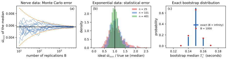
fig_8_s1. Download: PDF · SVG8.2 Bootstrap Variance Estimation
pp. 108–109 By Section 8.1 we can approximate \(\V_{\Fn}(T_n)\) by simulating from the distribution of \(T_n\) when the data come from \(\Fn\): draw \(X_1^*,\dots,X_n^*\) from \(\Fn\) and compute \(T_n^*=g(X_1^*,\dots,X_n^*)\). This is one draw. The book summarises the idea by two parallel lines, which in words read: in the real world, \(F\) generates \(X_1,\dots,X_n\), which give \(T_n\); in the bootstrap world, \(\Fn\) generates \(X_1^*,\dots,X_n^*\), which give \(T_n^*\). Every question about the sampling distribution of \(T_n\) under \(F\) is answered by the same question about \(T^*_n\) under \(\Fn\), and the bootstrap world is fully known, so it can be simulated.
Because \(\Fn\) puts mass \(1/n\) on each data point, a draw from \(\Fn\) is a draw of one data point at random; a bootstrap sample is \(n\) draws with replacement.
Algorithm 8.A (bootstrap variance estimation) p. 109, (8.1)
- Draw \(X_1^*,\dots,X_n^*\sim\Fn\), i.e. \(n\) times with replacement from the data.
- Compute \(T_n^*=g(X_1^*,\dots,X_n^*)\).
- Repeat steps 1 and 2 \(B\) times, giving \(T^*_{n,1},\dots,T^*_{n,B}\).
- Return
In the code: bootstrap(stat, data, B, rng) and v_boot(reps); paired data are resampled as pairs.
Filling the gap 8.3: resampling with replacement is sampling from \(\Fn\) pp. 108–109
Let \(J_1,\dots,J_n\) be iid uniform on \(\{1,\dots,n\}\), independent of the data, and \(X_i^*=X_{J_i}\). Conditionally on the data, \(X_1^*,\dots,X_n^*\) are iid with cdf \(\Fn\). Hence \(\vboot\) is the sample variance of \(B\) iid draws from the conditional law of \(T_n^*\), and \(\vboot\to\V_{\Fn}(T_n)\) as \(B\to\infty\) for almost every sequence of resamples.
Proof
Given the data, the \(J_i\) are independent, so the \(X_i^*=X_{J_i}\) are independent. For each \(i\),
\[ \P(X_i^*\le x\given X_1,\dots,X_n)=\sum_{j=1}^n\frac1n\,I(X_j\le x)=\Fn(x). \]Then \(T^*_{n,b}=g(X^*_{1,b},\dots,X^*_{n,b})\) for independent resamples \(b=1,\dots,B\) are iid draws from the conditional law of \(T^*_n\), which by definition is the law of \(T_n\) under \(\Fn\). That law has finite support (at most \(n^n\) points), so all its moments are finite, and the strong law of large numbers (Theorem 5.18) applied to \(T^*\) and \(T^{*2}\) gives \(\vboot\to\V_{\Fn}(T_n)\) almost surely in the resampling. ∎
The \(n^n\) equally likely index vectors \((J_1,\dots,J_n)\) collapse to \(\binom{2n-1}n\) distinct resamples, with multinomial weights (Exercise 8.4): 35 for \(n=4\), 77 558 760 for the 15 law schools, and about \(10^{479}\) for the 799 nerve times. Exact enumeration is out of the question beyond tiny \(n\), which is why step 2 is simulation.
Example 8.1 (the median). p. 109 To estimate the standard error of the sample median, compute the median of each of \(B\) resamples and take the standard deviation of the \(B\) values. The book stresses that two approximations are made,
\[ \V_F(T_n)\ \underset{\text{not so small}}{\approx}\ \V_{\Fn}(T_n)\ \underset{\text{small}}{\approx}\ \vboot, \]the first a statistical error that depends on \(n\), the second a simulation error that depends on \(B\). For the median both errors can be measured exactly.
Filling the gap 8.4: the two approximations, measured on the median p. 109
(a) The ideal bootstrap distribution of the median needs no simulation. Let \(n=2m-1\) be odd, so that the median of a resample is its \(m\)-th smallest value. For every data value \(v\) (ties allowed),
\[ \Ps\big(\med(X_1^*,\dots,X_n^*)\le v\big)=\P\big(\Bin(n,\Fn(v))\ge m\big). \](b) The statistical error is larger than for smooth statistics. For a smooth statistic (a smooth function of means), \(\V_{\Fn}(T_n)/\V_F(T_n)-1\) is of order \(n^{-1/2}\) in probability; for the median it is of order \(n^{-1/4}\) (Hall and Martin 1988), so the ideal bootstrap standard error of a median stays noticeably variable even for large samples.
Proof of (a), and the numbers
The resample's median is at most \(v\) exactly when at least \(m\) of the \(n\) draws are at most \(v\). Each draw is at most \(v\) with probability \(\Fn(v)\), independently of the others (Filling the gap 8.3), so the count of such draws is \(\Bin(n,\Fn(v))\). Taking differences of this cdf at consecutive distinct data values gives the probabilities. The companion course proves the same formula for distinct data in Result 4.6; ties only change \(j/n\) into \(\Fn(v)\). ∎
The nerve data. The 799 waiting times are recorded to 0.01 s and their median is 0.15. The exact bootstrap law of the median puts probabilities 0.0031, 0.1664, 0.6942, 0.1303 and 0.0059 on 0.13, 0.14, 0.15, 0.16 and 0.17 (and less than \(10^{-4}\) elsewhere), so the ideal bootstrap standard error is \(0.005767\). Figure 8.S1(a) shows simulated runs converging to it; Figure 8.S1(c) compares the exact law with 1000 replications.
Rate of the statistical error, checked. For exponential data the true variance of the median of \(n=2m-1\) observations is exact: by Rényi's representation \(X_{(k)}=\sum_{j=n-k+1}^{n}E_j/j\) with iid \(\Exp(1)\) variables \(E_j\), so \(\V(X_{(m)})=\sum_{j=m}^{n}j^{-2}\). Dividing the exact ideal bootstrap standard error by this truth, over 1000 samples, the standard deviation of the ratio is 0.37, 0.29, 0.23, 0.20 and 0.17 for \(n=21\), 51, 101, 201 and 401 (Figure 8.S5(b)). Over a twentyfold increase of \(n\) it falls by a factor 2.2, close to \(20^{1/4}=2.1\) and far from the \(20^{1/2}=4.5\) of a smooth statistic.
Example 8.2 (the skewness of the nerve data). pp. 109–110 The skewness \(\th=T(F)=\int(x-\mu)^3\,\d F(x)/\sigma^3\) measures asymmetry; it is 0 for a Normal law. Its plug-in estimate is
\[ \hth=T(\Fn)=\frac{n^{-1}\sum_{i=1}^n(X_i-\overline X_n)^3}{\hs^{\,3}}. \]For the nerve data, \(\hth=1.761\) (the book: 1.76). With \(B=1000\) the bootstrap gives \(\seboot=0.169\) in our run (the book: 0.16); the ideal value, from 200 000 replications, is 0.163. The jackknife gives 0.172 (Section 8.5.1) and the influence function, below, 0.164.
Filling the gap 8.5: why the bootstrap agrees with the delta method: the influence function of the skewness p. 110
For a functional \(T\), the influence function is the derivative in the direction of a point mass \(\delta_x\):
\[ L_F(x)=\lim_{\epsilon\downarrow0}\frac{T((1-\epsilon)F+\epsilon\delta_x)-T(F)}\epsilon. \]If \(T(\Fn)-T(F)\approx n^{-1}\sum_iL_F(X_i)\) (a first-order expansion of \(T\) at \(F\), which holds for smooth functionals), then \(\V(T(\Fn))\approx\E L_F(X)^2/n\), estimated by \(\hse^2=n^{-2}\sum_iL_{\Fn}(X_i)^2\): the nonparametric delta method. For the skewness,
\[ L_F(x)=\frac{(x-\mu)^3-\mu_3-3\sigma^2(x-\mu)}{\sigma^3}-\frac{3\mu_3}{2\sigma^5}\big((x-\mu)^2-\sigma^2\big), \]with \(\mu_3=\int(x-\mu)^3\,\d F\). For the nerve data this gives \(\hse=0.1635\), next to the ideal bootstrap 0.1629. The Chapter 7 notes develop the influence function and the nonparametric delta method in general (Filling the gap 7.12) and the standard error of the skewness by the ordinary delta method (Filling the gap 7.9); here is the short derivation for the skewness.
Derivation
Write \(F_\epsilon=(1-\epsilon)F+\epsilon\delta_x\) and differentiate at \(\epsilon=0\). The mean \(\mu(F_\epsilon)=(1-\epsilon)\mu+\epsilon x\) has derivative \(x-\mu\). For \(\sigma^2(F_\epsilon)=\int(y-\mu_\epsilon)^2\,\d F_\epsilon(y)\), the product rule gives two terms: moving the measure contributes \((x-\mu)^2-\sigma^2\), and moving the centre contributes \(-2\int(y-\mu)\,\d F(y)\cdot(x-\mu)=0\). So \(L_{\sigma^2}(x)=(x-\mu)^2-\sigma^2\). For \(\mu_3(F_\epsilon)=\int(y-\mu_\epsilon)^3\,\d F_\epsilon\), the measure contributes \((x-\mu)^3-\mu_3\) and the centre contributes \(-3\int(y-\mu)^2\,\d F\cdot(x-\mu)=-3\sigma^2(x-\mu)\). Finally \(\th=\mu_3(\sigma^2)^{-3/2}\), and the chain rule gives \(L_\th=L_{\mu_3}\sigma^{-3}-\tfrac32\mu_3\sigma^{-5}L_{\sigma^2}\), the display. Each piece has mean zero under \(F\), as an influence function must.
Why the bootstrap sees the same thing. In the bootstrap world the same expansion at \(\Fn\) reads \(T(\Fn^*)-T(\Fn)\approx n^{-1}\sum_iL_{\Fn}(X^*_i)\), with \(\Fn^*\) the empirical cdf of the resample, whose conditional variance is exactly \(n^{-2}\sum_iL_{\Fn}(X_i)^2\) (because \(\sum_iL_{\Fn}(X_i)=0\)). So to first order the ideal bootstrap variance is the delta-method variance; the bootstrap also captures the higher-order terms (skewness of \(\hth\), curvature of \(T\)) that the linear expansion drops. Making "\(\approx\)" rigorous needs a differentiability of \(T\) strong enough to control the remainder uniformly; Hadamard differentiability suffices (van der Vaart 1998, Chapter 20). ∎
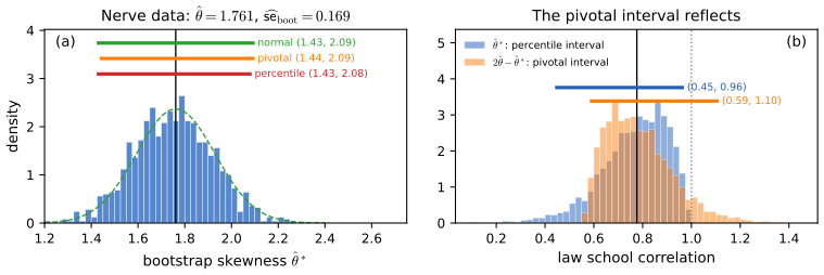
fig_8_s2. Download: PDF · SVGSee also (companion courses): the bootstrap standard error of any statistic in Applied Statistical Learning, Algorithm 5.2, and the Monte Carlo bootstrap in Statistical Methods for Modern Biology, Algorithm 4.3.
8.3 Bootstrap Confidence Intervals
p. 110 The book gives three ways to turn the replications into a confidence interval (Definition 6.D).
Method 1: the Normal interval. \(T_n\pm z_{\alpha/2}\,\seboot\). It is accurate only when the distribution of \(T_n\) is close to Normal.
\[ T_n\pm z_{\alpha/2}\,\seboot \tag{8.2} \]Method 2: the pivotal interval. Let \(\th=T(F)\), \(\hth=T(\Fn)\), and call \(R_n=\hth-\th\) the pivot, with cdf
\[ H(r)=\P_F(R_n\le r). \tag{8.3} \]If \(H\) were known, the interval \(C_n^\star=(a,b)\) with
\[ a=\hth-H^{-1}\Big(1-\frac\alpha2\Big),\qquad b=\hth-H^{-1}\Big(\frac\alpha2\Big) \tag{8.4} \]would have coverage exactly \(1-\alpha\). \(H\) is unknown, but its bootstrap estimate is
\[ \widehat H(r)=\frac1B\sum_{b=1}^BI\big(R^*_{n,b}\le r\big),\qquad R^*_{n,b}=\widehat\theta^*_{n,b}-\hth. \tag{8.5} \]Writing \(\widehat\theta^*_\beta\) for the \(\beta\) sample quantile of the replications, the \(\beta\) quantile of the \(R^*\) is \(\widehat\theta^*_\beta-\hth\), and substituting into (8.4) gives the bootstrap pivotal interval
\[ C_n=\Big(2\hth-\widehat\theta^*_{1-\alpha/2},\ 2\hth-\widehat\theta^*_{\alpha/2}\Big). \tag{8.6} \]Filling the gap 8.6: the exact pivotal interval, and why (8.6) is called the "basic" interval pp. 110–111
(a) If \(H\) is continuous, \(\P(a\le\th\le b)=1-\alpha\) exactly, with \(a,b\) from (8.4). The book's chain of equalities uses \(H(H^{-1}(p))=p\), which needs this continuity; for a discrete \(H\) (a median, say) the coverage can differ from \(1-\alpha\) either way.
(b) Sample quantiles are shift-equivariant, so \(r^*_\beta=\widehat\theta^*_\beta-\hth\) holds exactly (also for the linear-interpolation quantiles used in the code), and (8.6) follows from (8.4) with \(\widehat H\) for \(H\).
(c) (8.6) is the percentile interval of the reflected replications \(2\hth-\widehat\theta^*_{n,b}\). It is what one gets from the plug-in principle alone, applied to the law of \(\hth-\th\), with no further assumption; Davison and Hinkley (1997) call it the basic bootstrap interval.
Proof
(a) Since \(a=\hth-H^{-1}(1-\alpha/2)\), the event \(a\le\th\) is \(\hth-\th\le H^{-1}(1-\alpha/2)\), and \(\th\le b\) is \(\hth-\th\ge H^{-1}(\alpha/2)\). So
\[ \P(a\le\th\le b)=\P\Big(H^{-1}\big(\tfrac\alpha2\big)\le R_n\le H^{-1}\big(1-\tfrac\alpha2\big)\Big)=H\Big(H^{-1}\big(1-\tfrac\alpha2\big)\Big)-H\Big(H^{-1}\big(\tfrac\alpha2\big)-\Big). \]For continuous \(H\), \(H(H^{-1}(p))=p\) for \(0<p<1\) (the generalised inverse of Definition 2.5 lands on a point where \(H\) reaches \(p\)), and \(H(x-)=H(x)\); the coverage is \(1-\alpha/2-\alpha/2=1-\alpha\). If \(H\) has an atom at an endpoint, the closed interval gains the atom's mass and the coverage can exceed \(1-\alpha\); if \(H\) jumps over level \(p\), \(H(H^{-1}(p))>p\) and the coverage can be anything near \(1-\alpha\).
(b) Adding the constant \(-\hth\) to every replication adds it to every order statistic; the linear-interpolation quantile \(x_{(j)}+h(x_{(j+1)}-x_{(j)})\) is then shifted by the same constant because the difference \(x_{(j+1)}-x_{(j)}\) is unchanged. So \(\widehat H^{-1}(\beta)=r^*_\beta=\widehat\theta^*_\beta-\hth\), and \(a=\hth-r^*_{1-\alpha/2}=2\hth-\widehat\theta^*_{1-\alpha/2}\), \(b=2\hth-\widehat\theta^*_{\alpha/2}\).
(c) The \(\beta\)-quantile of the reflected values \(2\hth-\widehat\theta^*_{n,b}\) is \(2\hth-\widehat\theta^*_{1-\beta}\) (reflection reverses order), so their percentile interval is (8.6). ∎
Reading the reflection. Suppose the bootstrap distribution has a long right tail. The pivotal interval then stretches further to the left of \(\hth\): the logic is that if \(\hth^*\) overshoots \(\hth\) by a lot sometimes, then \(\hth\) overshoots \(\th\) by a lot sometimes, so \(\th\) may lie well below \(\hth\). The percentile interval stretches to the right instead. The two coincide when the bootstrap distribution is symmetric about \(\hth\), as for the nerve skewness (Figure 8.S2(a)), and differ sharply when it is skewed, as for the law school correlation, where the pivotal interval's upper end, 1.10, is impossible for a correlation (Figure 8.S2(b)).
Theorem 8.3 (consistency of the pivotal interval) p. 111
Under weak conditions on \(T(F)\), \(\P_F(T(F)\in C_n)\to1-\alpha\) as \(n\to\infty\), where \(C_n\) is (8.6).
Filling the gap 8.7: a proof of Theorem 8.3 for smooth functions of means p. 111
The book does not say what "weak conditions" are. Here is a complete proof in the most common setting, with the general statement after it.
Setting. \(X_i\in\R^k\) iid with mean \(\mu\), covariance \(\Sigma\) and \(\E\|X\|^3<\infty\); \(\th=g(\mu)\) and \(\hth=g(\overline X_n)\), where \(g\) is continuously differentiable near \(\mu\) with \(\tau^2=\nabla g(\mu)^\T\Sigma\nabla g(\mu)>0\). This covers the mean, the variance, the skewness, the correlation and ratios of means (each is a smooth function of a vector of sample moments). Let \(\widehat H_n(r)=\Ps(\sqrt n(\hth^*-\hth)\le r)\) be the ideal bootstrap cdf of the scaled pivot (\(B=\infty\)). Then, for almost every data sequence, \(\sup_r|\widehat H_n(r)-\Phi(r/\tau)|\to0\), and the coverage of (8.6) tends to \(1-\alpha\); so does that of the percentile interval. If \(B=B_n\to\infty\), the same holds with simulated quantiles.
Proof
Step 1 (real world). By the multivariate central limit theorem and the multivariate delta method (Theorem 5.12, Theorem 5.15), \(\sqrt n(\hth-\th)\convd\N(0,\tau^2)\). Since the limit cdf is continuous, the convergence of the cdfs \(H_n(r)=\P(\sqrt n(\hth-\th)\le r)\) to \(\Phi(r/\tau)\) is uniform in \(r\) (Pólya's theorem: pick finitely many points where the continuous limit increases by at most \(\epsilon\) between neighbours, and use monotonicity in between).
Step 2 (bootstrap world: the mean). Fix a vector \(c\in\R^k\) and the data. Conditionally, \(c^\T X_i^*\) are iid with mean \(c^\T\overline X_n\), variance \(c^\T\widehat\Sigma c\) (\(\widehat\Sigma\) the divisor-\(n\) sample covariance) and third absolute central moment \(\widehat\rho_c=n^{-1}\sum_j|c^\T(X_j-\overline X_n)|^3\). The Berry–Esseen inequality (Theorem 5.11), applied in the bootstrap world, gives
\[ \sup_x\Big|\Ps\big(\sqrt n\,c^\T(\overline X^*_n-\overline X_n)\le x\big)-\Phi\Big(\frac x{\sqrt{c^\T\widehat\Sigma c}}\Big)\Big|\le\frac{0.4748\,\widehat\rho_c}{(c^\T\widehat\Sigma c)^{3/2}\sqrt n}. \]By the strong law of large numbers (Theorem 5.18), \(\widehat\Sigma\to\Sigma\) and \(\widehat\rho_c\to\E|c^\T(X-\mu)|^3<\infty\) almost surely, so the right side tends to 0 whenever \(c^\T\Sigma c>0\) (when \(c^\T\Sigma c=0\), \(c^\T X\) is a.s. constant and both sides are degenerate). Taking \(c\) in a countable dense set, outside one null set of data sequences, the conditional characteristic functions of \(\sqrt n(\overline X^*_n-\overline X_n)\) converge to those of \(\N(0,\Sigma)\) at every such \(c\), hence (being uniformly equicontinuous, since the conditional second moments are bounded) at every \(c\): by the Cramér–Wold device, \(\sqrt n(\overline X^*_n-\overline X_n)\convd\N(0,\Sigma)\) conditionally, for almost every data sequence.
Step 3 (bootstrap world: the function). By the mean value theorem, \(\sqrt n(\hth^*-\hth)=\nabla g(\xi_n)^\T\sqrt n(\overline X_n^*-\overline X_n)\) with \(\xi_n\) on the segment between \(\overline X^*_n\) and \(\overline X_n\). Since \(\overline X_n\to\mu\) a.s. and \(\overline X^*_n-\overline X_n\to0\) in conditional probability (Step 2), \(\xi_n\to\mu\) in conditional probability, and \(\nabla g(\xi_n)\to\nabla g(\mu)\) by continuity. Slutsky's theorem in the bootstrap world gives \(\sqrt n(\hth^*-\hth)\convd\N(0,\tau^2)\) conditionally, and Pólya's theorem makes \(\widehat H_n\to\Phi(\cdot/\tau)\) uniform.
Step 4 (quantiles and coverage). If cdfs converge to a continuous, strictly increasing limit, their \(\beta\)-quantiles converge to the limit's \(\beta\)-quantile (for small \(\epsilon\), eventually \(\widehat H_n(q-\epsilon)<\beta<\widehat H_n(q+\epsilon)\)). So \(\hat h_\beta=\widehat H_n^{-1}(\beta)\to\tau\Phi^{-1}(\beta)\) a.s. The pivotal interval is \(\{\th:\hat h_{\alpha/2}\le\sqrt n(\hth-\th)\le\hat h_{1-\alpha/2}\}\), so its coverage is \(\P\big(\hat h_{\alpha/2}\le\sqrt n(\hth-\th)\le\hat h_{1-\alpha/2}\big)\). Since the \(\hat h\) converge a.s. to constants, Slutsky's theorem and Step 1 give the limit \(\P(-\tau z_{\alpha/2}\le\tau Z\le\tau z_{\alpha/2})=1-\alpha\). The percentile interval is \(\{\th:-\hat h_{1-\alpha/2}\le\sqrt n(\hth-\th)\le-\hat h_{\alpha/2}\}\), and because the limit \(\N(0,\tau^2)\) is symmetric, \(-\tau\Phi^{-1}(1-\alpha/2)=\tau\Phi^{-1}(\alpha/2)\): the same limit.
Step 5 (finite \(B\)). Conditionally on the data, the empirical cdf of \(B\) replications converges uniformly to \(\widehat H_n\) as \(B\to\infty\) (Glivenko–Cantelli, Theorem 7.4), and the quantile argument of Step 4 applies to it. ∎
Remarks. (i) Finite variance is enough for the mean (Bickel and Freedman 1981; Singh 1981), using Lindeberg's condition instead of Berry–Esseen; the companion course proves this in Result 4.7. (ii) In general the bootstrap is consistent for \(\sqrt n(T(\Fn)-T(F))\) whenever \(T\) is Hadamard differentiable at \(F\) (van der Vaart 1998, Theorem 23.9); this includes quantiles of a distribution with a positive continuous density at the quantile, so the bootstrap works for the median, where the jackknife does not (Filling the gap 8.11). (iii) The Normal interval (8.2) needs more: \(\sqrt n\,\seboot\to\tau\), a statement about the conditional variance, which convergence in distribution does not imply. It holds for smooth functions of means under enough moments, but can fail for heavy tails even when the bootstrap distribution is consistent (Ghosh et al. 1984). (iv) The bootstrap is not consistent when \(T\) is not smooth at \(F\): the maximum of Exercise 8.7 is the standard example (Filling the gap 8.12).
Method 3: the percentile interval. p. 111 The bootstrap percentile interval is
\[ C_n=\Big(\widehat\theta^*_{\alpha/2},\ \widehat\theta^*_{1-\alpha/2}\Big). \]Its justification is in Section 8.5.2 (and, corrected, in Filling the gap 8.9). In the code all three are returned by boot_intervals(theta, reps, alpha).
Example 8.4 (the nerve-data skewness). p. 111 The three 95% intervals, from the book and from our run with \(B=1000\) (Figure 8.S2(a)):
| Method | Book | Our run, \(B=1000\) | Ideal, \(B=200\,000\) |
|---|---|---|---|
| Normal | (1.44, 2.09) | (1.43, 2.09) | (1.44, 2.08) |
| Pivotal | (1.48, 2.11) | (1.44, 2.09) | (1.45, 2.09) |
| Percentile | (1.42, 2.03) | (1.43, 2.08) | (1.43, 2.07) |
The differences from the book are Monte Carlo noise of the size computed in Filling the gap 8.2 (endpoint standard deviation about 0.012 at \(B=1000\)). The book's remark that "all three intervals have the same level of accuracy" is made precise in the next box; it does not mean that they are accurate.
Filling the gap 8.8: how accurate are the three intervals? p. 111
Consistency (Theorem 8.3) says only that the coverage tends to \(1-\alpha\). How fast? For a smooth function of means with enough moments, the classical answers (Hall 1992, Chapter 3) are:
- For one-sided intervals (a single endpoint), the Normal, pivotal and percentile methods all have coverage error of order \(n^{-1/2}\).
- For two-sided equal-tailed intervals, all three have coverage error of order \(n^{-1}\): the \(n^{-1/2}\) errors of the two tails cancel. This is the precise sense of "the same level of accuracy".
- The studentized (bootstrap-\(t\)) interval, which bootstraps \((\hth-\th)/\hse\) instead of \(\hth-\th\), and Efron's BC\(_a\) interval have one-sided error of order \(n^{-1}\). These are the "more accurate" intervals the book mentions.
Where the orders come from (a sketch)
This is a sketch of Hall's argument, not a proof; the full treatment needs Edgeworth expansions with remainder bounds (Hall 1992, Chapters 2 and 3). Let \(S_n=\sqrt n(\hth-\th)/\tau\). Under smoothness and a non-lattice condition,
\[ \P(S_n\le x)=\Phi(x)+n^{-1/2}p(x)\phi(x)+O(n^{-1}), \]with \(p\) an even polynomial of degree 2 whose coefficients are moments of \(F\) (for the mean, \(p(x)=-\gamma(x^2-1)/6\), \(\gamma\) the skewness of \(X\)). In the bootstrap world the same expansion holds with \(\Fn\) for \(F\),
\[ \Ps(S^*_n\le x)=\Phi(x)+n^{-1/2}\hat p(x)\phi(x)+O_P(n^{-1}), \]where \(\hat p-p=O_P(n^{-1/2})\) because sample moments are \(\sqrt n\)-consistent. So for a standardised statistic the bootstrap is right to order \(n^{-1}\): it captures the skewness term that the Normal approximation misses.
The pivotal and percentile intervals bootstrap \(\hth-\th\) itself, whose scale \(\tau/\sqrt n\) is estimated in the bootstrap world by \(\hat\tau/\sqrt n\) with \(\hat\tau-\tau=O_P(n^{-1/2})\). Then
\[ \widehat H(r)-H(r)\approx\Phi(r\sqrt n/\hat\tau)-\Phi(r\sqrt n/\tau)=O_P(n^{-1/2}): \]one-sided errors of order \(n^{-1/2}\). For a two-sided interval the coverage is \(\P(S_n\le x_2)-\P(S_n<x_1)\); the \(n^{-1/2}\) terms are \(p(x)\phi(x)\) at the two ends and, with \(x_1\approx-x_2\) and \(p\phi\) even, they cancel, leaving \(O(n^{-1})\). The studentized pivot \((\hth-\th)/\hse\) has no unknown scale, so its bootstrap is right to order \(n^{-1}\) at each end. ∎
What the numbers say. Orders of magnitude say nothing about constants. For the mean of 25 exponential observations (demo, preset 3) the two-sided coverage is about 0.90, with the interval lying below \(\th\) in 8.5% of the data sets and above it in 1.3%: one-sided errors of 6 and 1 percentage points, as the \(n^{-1/2}\) term predicts for a skewed law. For the skewness of lognormal data (Exercise 8.2) all three intervals cover less than 26% even for \(n=200\), and they miss almost only on one side. The expansion's constants involve the sixth moment of \(F\), enormous for the lognormal, so the asymptotics are far away.
Example 8.5 (plasma cholesterol). p. 112 The book returns to the cholesterol data of its Example 7.15 (371 patients with chest pain, Scott et al. 1978) and bootstraps the difference of the two group medians with independent resampling within each group: the point estimate is 18.5 mg/dl, \(\seboot=7.42\), and the 95% intervals are Normal (3.7, 33.3), pivotal (5.0, 34.0) and percentile (5.0, 33.3), all excluding 0. Those data are not on the book's website, so the example cannot be reproduced. The same two-sample computation on a data set that is there, the LDL cholesterol (mmol/l) of the 462 men in coris.dat (the South African heart disease data of later chapters), split by coronary heart disease: the medians are 3.98 (302 men without) and 5.065 (160 men with), the difference is 1.085, \(\seboot=0.21\) (\(B=1000\)), and the intervals are Normal (0.68, 1.49), pivotal (0.68, 1.49) and percentile (0.68, 1.49). Using \(\pm2\,\seboot\), as the book's pseudocode does instead of \(\pm1.96\), gives (0.67, 1.50). As in the book, the intervals exclude 0, and as in the book this is an association: the men were sampled retrospectively by disease status, and nothing here says that LDL causes the disease.
Example 8.6 (the law school data). pp. 112–113 This is one of Efron's first illustrations of the bootstrap: average LSAT score and GPA for 15 law schools, with \(X_i=(Y_i,Z_i)\) and \(\th\) the correlation between \(Y\) and \(Z\), estimated by the sample correlation. The last school's GPA is printed as 3.96; the author's errata corrects it to 2.96, and only 2.96 reproduces the quoted estimate (with 3.96 the correlation would be 0.546). Then \(\hth=0.776\); our run with \(B=1000\) gives \(\seboot=0.134\) (book 0.137; ideal 0.133) and the intervals Normal (0.51, 1.04), percentile (0.45, 0.95) and pivotal (0.60, 1.11). The book's percentile interval (0.46, 0.96) agrees. Its Normal interval is printed as (0.51, 1.00): the upper end \(0.776+2(0.137)=1.05\) has evidently been cut at the largest possible correlation, 1. With \(n=15\) the bootstrap distribution is strongly skewed (Figure 8.1(b)), the intervals disagree, and the book rightly warns against reading too much into any of them. For comparison, the classical interval for a Normal population, through Fisher's transformation \(\tanh\big(\operatorname{artanh}\hth\pm1.96/\sqrt{n-3}\big)\), is (0.44, 0.92).
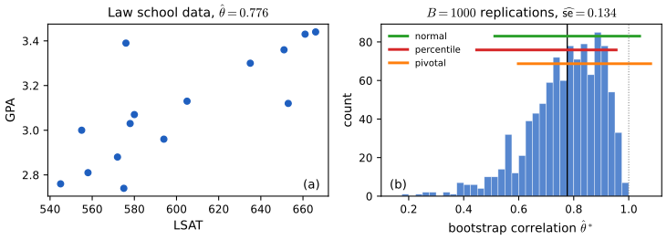
fig_8_1. Download: PDF · SVGExample 8.7 (bioequivalence of hormone patches). pp. 113–115 Eight subjects each received a placebo, an old patch and a new patch. With \(Z=\text{old}-\text{placebo}\) and \(Y=\text{new}-\text{old}\), the regulator's criterion for bioequivalence is \(|\th|\le0.20\) with \(\th=\E_F(Y)/\E_F(Z)\). The plug-in estimate is \(\hth=\overline Y/\overline Z=-452.25/6342.375=-0.0713\). Resampling the eight subjects (pairs \((Y_i,Z_i)\) together), our run gives \(\seboot=0.106\) (book 0.105; ideal 0.102) and the intervals Normal (\(-0.28\), 0.14), percentile (\(-0.24\), 0.19) and pivotal (\(-0.33\), 0.09). The book's interval (\(-0.24\), 0.15) is a percentile interval; the ideal one is (\(-0.23\), 0.17), and the upper endpoint varies from run to run by about 0.014 at \(B=1000\) (demo), which explains the difference. None of the intervals lies inside \((-0.2,0.2)\), so bioequivalence is not demonstrated at this level.
Two remarks. First, the logic "declare equivalence if the \(1-2\alpha\) interval lies inside the margin" is a test: it rejects non-equivalence at level \(\alpha\) by two one-sided tests, each at level \(\alpha\), so the book's 95% interval corresponds to a 2.5%-level test. Second, the delta method for a ratio, \(\hse^2=n^{-2}\sum_i\{(Y_i-\overline Y)-\hth(Z_i-\overline Z)\}^2/\overline Z^{\,2}\) (the influence-function recipe of Filling the gap 8.5), gives 0.098, a little below the bootstrap: with eight subjects the higher-order terms matter.
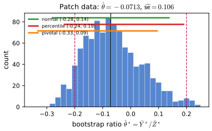
fig_8_2. Download: PDF · SVGSee also (companion courses): bootstrap estimates of prediction error in Statistical Learning: Theory and Methods, Section 7.11 (demo: the .632 estimator), and the bootstrap as an approximate posterior in Section 8.4 there.
8.4 Bibliographic Remarks
p. 115 The bootstrap was introduced by Efron (1979). Book-length treatments are Efron and Tibshirani (1993), Davison and Hinkley (1997), Hall (1992) and Shao and Tu (1995); Section 3.6 of van der Vaart and Wellner (1996) gives the empirical-process theory. For the arguments used in these notes: Bickel and Freedman (1981) and Singh (1981) for the consistency of the bootstrap of a mean, Hall (1992) for the accuracy of bootstrap intervals, van der Vaart (1998, Chapters 20 and 23) for influence functions and the functional delta method, Efron and Stein (1981) and Efron (1982) for the jackknife.
8.5 Appendix
8.5.1 The Jackknife
pp. 115–116 The jackknife, due to Quenouille (1949), is an older and cheaper way to estimate a standard error. Let \(T_{(-i)}\) be the statistic computed with the \(i\)-th observation removed and \(\overline T_n=n^{-1}\sum_iT_{(-i)}\). The jackknife estimates are
\[ \vjack=\frac{n-1}n\sum_{i=1}^n\big(T_{(-i)}-\overline T_n\big)^2,\qquad\sejack=\sqrt{\vjack}. \]The book states, without proof, that under suitable conditions \(\vjack/\V(T_n)\convp1\), and that, unlike the bootstrap, the jackknife does not consistently estimate the standard error of sample quantiles. The next two boxes prove both statements. In the code: jackknife(stat, data).
Filling the gap 8.10: why the factor \((n-1)/n\): the jackknife is exact for the mean and consistent for smooth statistics p. 116
(a) For \(T_n=\overline X_n\), \(\vjack=s^2/n\) exactly, an unbiased estimate of \(\V(\overline X_n)\).
(b) If \(T_n=g(\overline X_n)\) with \(X_i\in\R^k\), \(\E\|X\|^4<\infty\) and \(g\) twice continuously differentiable near \(\mu\) with \(\tau^2=\nabla g(\mu)^\T\Sigma\nabla g(\mu)>0\), then \(n\,\vjack\to\tau^2\) almost surely, where \(\tau^2/n\) is the asymptotic variance of \(T_n\); so \(\vjack/\V(T_n)\to1\) whenever \(n\V(T_n)\to\tau^2\), which holds under mild growth conditions on \(g\).
(c) (Efron and Stein 1981.) For any symmetric statistic with finite variance, \(\E\,\vjack\ge\frac{n-1}n\V(T_{n-1})\): on average the jackknife overestimates the variance of the statistic based on \(n-1\) observations. Figure 8.S5(c) shows this upward lean for the skewness.
Proof of (a) and (b)
(a) \(T_{(-i)}=(n\overline X_n-X_i)/(n-1)\), so \(\overline T_n=\overline X_n\) and \(T_{(-i)}-\overline T_n=(\overline X_n-X_i)/(n-1)\). Hence \(\vjack=\frac{n-1}n\cdot\frac{\sum_i(X_i-\overline X_n)^2}{(n-1)^2}=\frac{s^2}n\). The factor \((n-1)/n\) is chosen precisely to make this come out: leave-one-out values are \(n-1\) times less variable than the observations, and the factor undoes that. For the nerve data, \(\sejack=s/\sqrt n=0.0074006\).
(b) Write \(\overline X_{(-i)}\) for the leave-one-out means, so \(\overline X_{(-i)}-\overline X_n=(\overline X_n-X_i)/(n-1)\). Because \(\E\|X\|<\infty\), \(\max_i\|X_i\|/n\to0\) almost surely (Borel–Cantelli: \(\sum_n\P(\|X_n\|>\epsilon n)\le\E\|X\|/\epsilon\)), so all leave-one-out means eventually lie in the neighbourhood where \(g\) is \(C^2\). Taylor's theorem gives \(T_{(-i)}=g(\overline X_n)+a_i+r_i\) with
\[ a_i=\nabla g(\overline X_n)^\T(\overline X_{(-i)}-\overline X_n),\qquad|r_i|\le\frac{M\|X_i-\overline X_n\|^2}{(n-1)^2}. \]The linear parts have mean zero over \(i\), and by (a) applied to the scalars \(\nabla g(\overline X_n)^\T X_i\),
\[ n\cdot\frac{n-1}n\sum_i(a_i-\bar a)^2=\nabla g(\overline X_n)^\T S\,\nabla g(\overline X_n)\to\tau^2\quad\text{a.s.}, \]with \(S\) the sample covariance (strong law). The remainders are negligible:
\[ n\sum_ir_i^2\le\frac{M^2n}{(n-1)^4}\sum_i\|X_i-\overline X_n\|^4=O(n^{-2})\cdot\frac1n\sum_i\|X_i-\overline X_n\|^4\to0 \]almost surely, by the strong law and \(\E\|X\|^4<\infty\); the cross term is controlled by the Cauchy–Schwarz inequality. So \(n\,\vjack\to\tau^2\). ∎
Part (c) is quoted from Efron and Stein (1981); its proof uses the orthogonal (Hoeffding) decomposition of a symmetric statistic and is not needed here. The argument in (b) also shows what the jackknife really computes: \(T_{(-i)}-\overline T_n\approx-L_{\Fn}(X_i)/(n-1)\), so \(\vjack\approx n^{-2}\sum_iL_{\Fn}(X_i)^2\), the nonparametric delta method of Filling the gap 8.5. It works exactly when the statistic is smooth enough for a linear approximation to be accurate on the tiny perturbations \(\Fn\to\Fn^{(-i)}\).
Filling the gap 8.11: the jackknife fails for the median p. 116
Let \(F\) have a density \(f\), continuous and positive at the median \(\xi\), so that \(n\V(\med)\to1/(4f(\xi)^2)\) under mild moment conditions. Then \(\vjack\) divided by \(1/(4nf(\xi)^2)\) converges in distribution, not in probability:
\[ n\text{ even:}\ \ \frac{\sejack}{1/(2\sqrt nf(\xi))}\convd E_1\sim\Exp(1),\qquad n\text{ odd:}\ \ \frac{\sejack}{1/(2\sqrt nf(\xi))}\convd\frac{E_1+E_2}2\sim\tfrac12\Gam(2,1), \]with \(E_1,E_2\) iid \(\Exp(1)\). Both limits have mean 1 but standard deviations 1 and \(1/\sqrt2=0.71\): the jackknife standard error is about right on average and useless for any single data set. For the variance itself the limits have means \(\E E_1^2=2\) and \(\E\{(E_1+E_2)/2\}^2=1.5\). With ties the jackknife can even return 0: for the nerve data the three middle order statistics all equal 0.15, so every leave-one-out median is 0.15 and \(\sejack=0\), while the bootstrap gives 0.0058.
Proof
The leave-one-out medians. Let \(X_{(1)}\le\dots\le X_{(n)}\) be the order statistics (with ties, assign ranks arbitrarily; the values below do not depend on the choice).
Even \(n=2m\). Removing an observation of rank \(\le m\) leaves \(2m-1\) values whose median (the \(m\)-th smallest) is \(X_{(m+1)}\); removing one of rank \(\ge m+1\) leaves median \(X_{(m)}\). So \(m\) of the \(T_{(-i)}\) equal \(X_{(m+1)}\) and \(m\) equal \(X_{(m)}\); \(\overline T_n\) is their midpoint and, with \(D=X_{(m+1)}-X_{(m)}\),
\[ \vjack=\frac{n-1}n\cdot n\cdot\frac{D^2}4=\frac{(n-1)D^2}4. \]Odd \(n=2m+1\). Removing rank \(\le m\) gives \((X_{(m+1)}+X_{(m+2)})/2\), removing rank \(\ge m+2\) gives \((X_{(m)}+X_{(m+1)})/2\), and removing rank \(m+1\) gives \((X_{(m)}+X_{(m+2)})/2\). With the spacings \(D_1=X_{(m+1)}-X_{(m)}\) and \(D_2=X_{(m+2)}-X_{(m+1)}\), the values are, up to a common shift, \((D_1+D_2)/2\) (\(m\) times), 0 (\(m\) times) and \(D_2/2\) (once). Their sum of squared deviations is
\[ \frac m4(D_1+D_2)^2+\frac{D_2^2}4-\frac1n\Big(\frac m2(D_1+D_2)+\frac{D_2}2\Big)^2=\frac{m(m+1)}{4n}(D_1+D_2)^2+O(D_1^2+D_2^2), \]and \(m(m+1)/(4n)=n/16+O(1)\); so \(\vjack=\frac{n}{16}(D_1+D_2)^2\,(1+O_P(1/n))\).
The spacings. Write \(X_{(k)}=F^{-1}(U_{(k)})\) with \(U_{(k)}\) uniform order statistics (Result 2.4). Uniform order statistics have the representation \(U_{(k)}=\Gamma_k/\Gamma_{n+1}\) with \(\Gamma_k=E_1+\dots+E_k\), iid \(\Exp(1)\) variables; so
\[ n\big(U_{(m+1)}-U_{(m)},\,U_{(m+2)}-U_{(m+1)}\big)=\frac n{\Gamma_{n+1}}(E_{m+1},E_{m+2}), \]and \(n/\Gamma_{n+1}\to1\) almost surely: the two scaled middle spacings converge jointly in distribution to two iid \(\Exp(1)\) variables. By the mean value theorem, \(D_j=(U\text{-spacing})/f(\eta_j)\) with \(\eta_j\) between neighbouring middle order statistics, which converge to \(\xi\) in probability; by continuity of \(f\), \(nD_j\convd E_j/f(\xi)\) jointly.
Conclusion.
\[ n\text{ even: }n\vjack=\frac{n-1}{4n}(nD)^2\convd\frac{E_1^2}{4f(\xi)^2};\qquad n\text{ odd: }n\vjack\approx\frac{(nD_1+nD_2)^2}{16}\convd\frac{(E_1+E_2)^2}{16f(\xi)^2}. \]Dividing by \(1/(4f(\xi)^2)\) and taking square roots (continuous mapping) gives the two limits. Since the limits are non-degenerate, \(\vjack/\V(\med)\) does not converge in probability to 1. ∎
Checked by simulation. For exponential data with \(n=400\), the mean of \(\vjack/\V\) over 1500 samples is 2.13 and the standard deviation of \(\sejack/\se\) is 1.04; for \(n=401\) they are 1.50 and 0.70 (Figure 8.S5(a), (b)). Why the bootstrap succeeds. Deleting one observation moves the median by one spacing, of order \(1/n\), and the size of a single spacing is an \(\Exp(1)\)-like random variable; the jackknife sees only that. Resampling moves the median by order \(1/\sqrt n\), over many spacings, so their randomness averages out (Filling the gap 8.4; Theorem 8.3, remark (ii)).
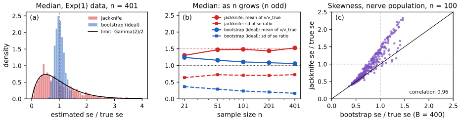
fig_8_s5. Download: PDF · SVG8.5.2 Justification for the Percentile Interval
p. 116 Suppose there is a monotone transformation \(U=m(T)\) with \(U\sim\N(\phi,c^2)\), \(\phi=m(\th)\); we need not know \(m\), only that it exists. The book shows that the percentile interval then has coverage exactly \(1-\alpha\). One step of its argument has a slip (the bootstrap quantiles are centred at \(U\), not at \(\phi\)), and one assumption is left implicit (the same transformation must also normalise the bootstrap replications). Here is the argument with both repaired.
Filling the gap 8.9: the percentile interval, correctly, and why it respects transformations p. 116
(a) Let \(m\) be strictly increasing and suppose that (i) \(U=m(\hth)\sim\N(\phi,c^2)\) with \(\phi=m(\th)\), and (ii) in the bootstrap world \(U^*=m(\hth^*)\sim\N(U,c^2)\) given the data. Then the ideal percentile interval has coverage exactly \(1-\alpha\).
(b) For every strictly increasing \(m\), the ideal percentile interval for \(m(\th)\) computed from the replications \(m(\hth^*)\) is \(\big(m(\widehat\theta^*_{\alpha/2}),m(\widehat\theta^*_{1-\alpha/2})\big)\): the percentile method is transformation-respecting. The pivotal interval is not, and it need not even stay in the parameter space.
Proof
(b) first. For a strictly increasing \(m\), \(m(\hth^*)\le m(t)\) if and only if \(\hth^*\le t\), so the generalised-inverse \(\beta\)-quantile of \(m(\hth^*)\) is \(m\) of that of \(\hth^*\). (With linear interpolation between order statistics this holds only approximately, because \(m\) of an average is not the average of the \(m\) values; the discrepancy vanishes as \(B\to\infty\) for a continuous bootstrap law.)
(a) By (ii), the \(\beta\)-quantile of \(U^*\) is \(u^*_\beta=U+c\,\Phi^{-1}(\beta)\); in particular \(u^*_{\alpha/2}=U-cz_{\alpha/2}\) and \(u^*_{1-\alpha/2}=U+cz_{\alpha/2}\). (The book writes \(\phi\) instead of \(U\) here; with \(\phi\) the interval would not be random at all.) By (b), \(m(\widehat\theta^*_\beta)=u^*_\beta\). Since \(m\) is increasing,
\[ \P\big(\widehat\theta^*_{\alpha/2}\le\th\le\widehat\theta^*_{1-\alpha/2}\big)=\P\big(u^*_{\alpha/2}\le\phi\le u^*_{1-\alpha/2}\big)=\P\Big(-z_{\alpha/2}\le\frac{U-\phi}c\le z_{\alpha/2}\Big)=1-\alpha. \]The argument needs neither \(m\) nor \(c\) to be known: the bootstrap finds them implicitly. If only approximate normalising transformations exist, the coverage is approximately \(1-\alpha\); if \(m(\hth)\) is biased or its variance depends on \(\phi\), the BC and BC\(_a\) corrections of Efron (1987) adjust the percentiles. ∎
The law school example. For a correlation, Fisher's \(m(r)=\operatorname{artanh}r\) is approximately normalising with \(c^2\approx1/(n-3)\). The percentile interval (0.46, 0.96) automatically behaves as if it had used \(m\), and lies in \([-1,1]\) because every replication does. The pivotal interval reflects the left-skewed bootstrap distribution about \(\hth\) and ends at 1.10, outside the parameter space (Figure 8.S2(b)).
Supplement: the parametric bootstrap, and where the nonparametric bootstrap fails
Section 9.11 of the book introduces the parametric bootstrap: in a parametric model \(\{f(x;\th)\}\), draw the resamples from \(f(x;\hth)\) instead of \(\Fn\). It belongs here because it rescues the one exercise of this chapter where the nonparametric bootstrap breaks down.
Filling the gap 8.12: the maximum of uniform data p. 118, Exercise 8.7; p. 134, Section 9.11
Let \(X_i\sim\Unif(0,\th)\) and \(\hth=\max_iX_i\). Then (a) \(\P(\hth=\th)=0\) and \(n(\th-\hth)/\th\convd\Exp(1)\); (b) for the nonparametric bootstrap, \(\Ps(\hth^*=\hth)=1-(1-1/n)^n\), which tends to \(1-e^{-1}\approx0.632\), so the bootstrap law of \(n(\hth-\hth^*)/\hth\) keeps an atom of mass about 0.632 at 0 and does not converge to \(\Exp(1)\): the bootstrap is inconsistent; (c) the parametric bootstrap, drawing from \(\Unif(0,\hth)\), reproduces the law of \(\hth/\th\) exactly.
Proof
(a) \(\hth\) has the continuous cdf \((x/\th)^n\) on \([0,\th]\) (Result 2.21), so \(\P(\hth=\th)=0\), and for \(t\ge0\)
\[ \P\big(n(\th-\hth)/\th>t\big)=\P\big(\hth<\th(1-t/n)\big)=(1-t/n)^n\to e^{-t}. \](b) \(\hth^*<\hth\) exactly when none of the \(n\) draws hits the (a.s. unique) largest observation; each draw misses it with probability \(1-1/n\), independently, so \(\Ps(\hth^*=\hth)=1-(1-1/n)^n\). Since \(\log(1-1/n)^n=n\log(1-1/n)\to-1\), this tends to \(1-e^{-1}=0.6321\) (for \(n=50\) it is 0.6358). A sequence of laws with an atom of mass at least 0.6 at 0 cannot converge to the continuous \(\Exp(1)\), whose cdf at \(0\) is 0.
(c) If \(X^*_i\sim\Unif(0,\hth)\) given the data, then \(\hth^*/\hth\) has cdf \(x^n\) on \([0,1]\), the same as the law of \(\hth/\th\) under any \(\th\). So \(\hth/\th\) is an exact pivot, the parametric bootstrap estimates its law without error, and \(\big(\hth/(1-\alpha/2)^{1/n},\ \hth/(\alpha/2)^{1/n}\big)\) is an exact \(1-\alpha\) interval. ∎
The lesson. The nonparametric bootstrap imitates \(F\) by \(\Fn\), which works when the statistic depends smoothly on the distribution (Filling the gap 8.7, remark (ii)). The maximum depends on the extreme upper tail, where \(\Fn\) has no information beyond the largest observation; its fluctuations are of order \(1/n\), not \(1/\sqrt n\), and its limit is not Normal. Drawing smaller resamples (the "\(m\) out of \(n\)" bootstrap, with \(m\to\infty\), \(m/n\to0\)) restores consistency; using the model, as in (c), does better still.
See also (companion courses): the parametric bootstrap for a smoothing spline and its agreement with least squares in Statistical Learning: Theory and Methods, Result 8.1; the probability 0.632 in Applied Statistical Learning, Result 5.3.
Notes on the book
Three slips of Chapter 8 are in the author's errata lists; four more points are mine, each with the evidence.
Page 107: the terms of \(\hs^2\) should be squared
The plug-in variance is \(\hs^2=n^{-1}\sum_i(X_i-\overline X_n)^2\); the book prints the terms without the square (which would make it identically 0). Listed in the author's errata (second printing).
Page 108: \(\overline Y_n\) should be \(\overline Y_B\), and \(\d F\) should be \(\d G\)
In Section 8.1 the simulated values are \(Y_1,\dots,Y_B\), so their mean is \(\overline Y_B\); the \(\overline Y_n\) of lines 3, 5 and 6 is listed in the author's errata (second printing). Not listed: in the last display the limits are written \(\int y^2\,\d F(y)-(\int y\,\d F(y))^2\), but the \(Y_j\) are drawn from \(G\), so both integrals should be with respect to \(G\).
Page 113: the last GPA should be 2.96, not 3.96
Listed in the author's errata. Evidence: with 2.96 the sample correlation is 0.7764, the book's 0.776; with 3.96 it would be 0.546.
Page 113: the Normal interval for the law school correlation
The book gives \(.78\pm2\hse=(.51,1.00)\) with \(\hse=.137\), but \(0.776+2(0.137)=1.05\). The printed upper end has evidently been truncated at 1, the largest possible correlation. That is a sensible thing to do, but the text does not say so, and it hides the point that the Normal interval, like the pivotal one, can leave the parameter space (Filling the gap 8.9). Not in the errata lists.
Page 116, Section 8.5.2: the bootstrap quantiles are centred at \(U\), not \(\phi\)
The argument states "\(u^*_{\alpha/2}=\phi-z_{\alpha/2}c\)" and "\(u^*_{1-\alpha/2}=\phi+z_{\alpha/2}c\)". These cannot be right: \(\phi=m(\th)\) is a fixed unknown number, so the interval would not be random and its "coverage" would be 0 or 1. The quantiles of the bootstrap replications \(U^*\) are \(U\mp z_{\alpha/2}c\), and that is what the next display of the book actually uses. The argument also needs the assumption, not stated, that \(m(\hth^*)\sim\N(m(\hth),c^2)\) in the bootstrap world (Filling the gap 8.9). Not in the errata lists.
Page 118, Exercise 8.8: the formula for \(\vboot\) is missing a term
The exercise asks to show \(\vboot=4\overline X_n^2\hat\alpha_2/n+4\overline X_n\hat\alpha_3/n^2+\hat\alpha_4/n^3\) for \(T_n=\overline X_n^2\), with \(\hat\alpha_k=n^{-1}\sum_i|X_i-\overline X_n|^k\). The exact ideal bootstrap variance is
\[ \Vs\big(\overline X^{*2}_n\big)=\frac{4\overline X_n^2\hat\alpha_2}n+\frac{4\overline X_n\hat\alpha_3}{n^2}+\frac{\hat\alpha_4}{n^3}+\frac{(2n-3)\hat\alpha_2^2}{n^3}, \]where \(\hat\alpha_3\) must be the signed third central moment \(n^{-1}\sum_i(X_i-\overline X_n)^3\) (with absolute values the formula is wrong for left-skewed data). Evidence: for the four values 1, 2.5, 4, 7.5, exact enumeration of all \(4^4=256\) equally likely resamples gives \(\Vs(\overline X^{*2}_n)=92.4144\); the corrected formula gives 92.4144 and the book's 89.7750. The missing term is of order \(n^{-2}\), so the book's expression is correct to the leading orders, but it is not an identity. Derivation in the solution. Not in the errata lists.
8.6 Exercises
All eight exercises of Chapter 8 (Wasserman, 2004, pp. 116–118), restated in my own words, with complete solutions (hidden). Computational answers come from ch08_bootstrap.py.
Exercise 8.1. For the law school data of Example 8.6, compute the plug-in estimate of the correlation, its bootstrap standard error, and 95% Normal, pivotal and percentile intervals.
Solution
With the corrected GPA 2.96, \(\hth=0.7764\). With \(B=1000\) (seed of Figure 8.1): \(\seboot=0.134\); Normal \(0.776\pm1.96(0.134)=(0.51,1.04)\); pivotal \((2\hth-\widehat\theta^*_{.975},2\hth-\widehat\theta^*_{.025})=(0.60,1.11)\); percentile \((\widehat\theta^*_{.025},\widehat\theta^*_{.975})=(0.45,0.95)\). The ideal values (200 000 replications) are \(\seboot=0.133\) and percentile \((0.46,0.96)\), pivotal \((0.59,1.09)\). The jackknife gives \(\sejack=0.143\). The bootstrap distribution is strongly skewed to the left (a correlation cannot exceed 1, and fifteen points rarely produce a perfect line), so the three intervals disagree: the percentile interval is shifted down, the pivotal interval up and past 1. Only the percentile interval respects the range of a correlation (Filling the gap 8.9); a Normal-theory interval via Fisher's transformation gives (0.44, 0.92), close to the percentile one.
Exercise 8.2 (simulation). Take \(n=50\), \(Y_i\sim\N(0,1)\), \(X_i=e^{Y_i}\), and \(\th\) the skewness of \(X\). Build the three bootstrap 95% intervals from one data set, repeat many times, and estimate the true coverage of each.
Solution
The target. For \(X=e^Y\), \(\E X^k=e^{k^2/2}\). Writing \(w=e^{\sigma^2}=e\), the central moments give the skewness
\[ \th=(w+2)\sqrt{w-1}=(e+2)\sqrt{e-1}=6.185. \]The experiment. 1000 data sets, \(B=1000\) each (
coverage_ex2), for \(n=25,50,100,200\):\(n\) Normal Pivotal Percentile \(\th\) above the interval (Normal / pivotal / percentile) 25 0.047 0.112 0.000 0.953 / 0.888 / 1.000 50 0.131 0.157 0.029 0.869 / 0.838 / 0.971 100 0.197 0.212 0.129 0.803 / 0.759 / 0.871 200 0.255 0.249 0.178 0.745 / 0.711 / 0.822 At \(n=50\) the nominal 95% intervals cover 13%, 16% and 3% of the time, and when they miss, \(\th\) lies above them (Monte Carlo standard errors about 0.01). Why. The plug-in skewness of \(n\) numbers is at most \((n-2)/\sqrt{n-1}\) (6.86 for \(n=50\)), so it can barely reach 6.19 at all; and it depends on the extreme right tail of a lognormal law, which 50 observations rarely sample. Its distribution is concentrated far below \(\th\), and the bootstrap, which can only resample the observed values, inherits that bias and cannot detect it. The theory of Filling the gap 8.7 and 8.8 does apply (the lognormal has all moments), but its constants involve sixth moments of \(X\), which are \(e^{18}\)-sized, so "large \(n\)" means very large indeed. The pivotal interval does least badly because reflecting a right-skewed bootstrap distribution pushes its upper end up.
Exercise 8.3 (simulation). Take \(n=25\), \(X_i\sim t_3\), and \(\th=(q_{.75}-q_{.25})/1.34\), with \(q_p\) the \(p\)-th quantile. Compare the coverage and length of the Normal interval with bootstrap se, the percentile interval and the pivotal interval.
Solution
The target. The \(t_3\) law is symmetric, so \(q_{.25}=-q_{.75}\) and \(\th=2t_{3,.75}/1.34=2(0.76489)/1.34=1.1416\). (The constant 1.34 makes \(\th=\sigma\) for a Normal law, since \(2\Phi^{-1}(0.75)=1.349\).) Sample quantiles are by linear interpolation (
iqr_scale).The experiment. 1000 data sets, \(B=1000\) (
coverage_ex3):Method Coverage \(\th\) above / below Mean length Median length Normal 0.962 0.034 / 0.004 1.336 1.277 Pivotal 0.853 0.120 / 0.027 1.297 1.245 Percentile 0.979 0.021 / 0.000 1.297 1.245 The percentile and pivotal intervals have exactly the same length (one is the reflection of the other), but very different coverage: the bootstrap distribution of a scaled IQR from 25 heavy-tailed points is skewed to the right, the percentile interval inherits the right skew of the sampling distribution (good), and the pivotal interval reflects it to the left (bad), so it misses above \(\th\) 12% of the time. The Normal interval is slightly longer and close to nominal. The intervals are long (more than the target itself): with 25 observations from a law whose third and higher moments are infinite, a scale is poorly determined. Monte Carlo standard error of the coverages: about 0.006 to 0.011.
Exercise 8.4. If \(X_1,\dots,X_n\) are distinct, show that there are \(\binom{2n-1}n\) distinct bootstrap samples.
Solution
A bootstrap sample, as a data set, is determined by how many times each \(X_j\) appears: a vector \((k_1,\dots,k_n)\) of non-negative integers with \(k_1+\dots+k_n=n\) (the order of the draws does not change any statistic of an iid sample). Distinct data make distinct count vectors give distinct samples. Count the vectors by "stars and bars": write \(n\) stars (the draws) and \(n-1\) bars (separating the \(n\) buckets) in a row of \(2n-1\) symbols; \(k_j\) is the number of stars between the \((j-1)\)-th and \(j\)-th bars. Every arrangement gives one vector and conversely, and an arrangement is a choice of the \(n\) star positions among \(2n-1\): \(\binom{2n-1}n\). Examples: 3, 10, 35 and 126 for \(n=2,3,4,5\) (checked by enumeration); 77 558 760 for \(n=15\). The samples are not equally likely: the count vector has the multinomial probability \(\frac{n!}{k_1!\cdots k_n!}n^{-n}\), largest for the vector with every \(k_j=1\) (the original sample), whose probability \(n!/n^n\) is still tiny (\(\approx\sqrt{2\pi n}\,e^{-n}\)).
Exercise 8.5. For distinct observations and a bootstrap sample with mean \(\overline X^*_n\), find \(\E(\overline X^*_n\given X_1,\dots,X_n)\), \(\V(\overline X^*_n\given X_1,\dots,X_n)\), \(\E(\overline X^*_n)\) and \(\V(\overline X^*_n)\).
Solution
Conditionally, the \(X_i^*\) are iid with mean \(\overline X_n\) and variance \(\hs^2\) (Filling the gap 8.1), so \(\E(\overline X^*_n\given X)=\overline X_n\) and \(\V(\overline X^*_n\given X)=\hs^2/n\), with \(\hs^2=n^{-1}\sum_i(X_i-\overline X_n)^2\). Unconditionally (data iid with mean \(\mu\), variance \(\sigma^2\)), the tower rule gives \(\E\overline X^*_n=\E\overline X_n=\mu\). By the law of total variance,
\[ \V(\overline X^*_n)=\V\big(\E(\overline X^*_n\given X)\big)+\E\big(\V(\overline X^*_n\given X)\big)=\frac{\sigma^2}n+\frac{\E\hs^2}n=\frac{\sigma^2}n+\frac{(n-1)\sigma^2}{n^2}=\frac{(2n-1)\sigma^2}{n^2}, \]using \(\E\hs^2=\frac{n-1}n\sigma^2\) (Result 3.7). So a bootstrap mean varies about twice as much as a sample mean, unconditionally: once from the data, once from the resampling. The bootstrap uses only the conditional variance, which estimates \(\sigma^2/n\). For the nerve data \(\hs^2/n=5.470\times10^{-5}\).
Exercise 8.6 (computer experiment). With \(X_i\sim\N(\mu,1)\), \(\th=e^\mu\) and \(\hth=e^{\overline X}\), simulate \(n=100\) observations with \(\mu=5\). (a) Find the bootstrap se and a 95% interval for \(\th\). (b) Plot a histogram of the bootstrap replications and compare it with the true sampling distribution of \(\hth\).
Solution
Our data set (
fig_8_s6): \(\overline X=4.9995\), \(\hth=148.34\) (truth \(e^5=148.41\)). With \(B=2000\): \(\seboot=15.8\); Normal (117.3, 179.4), pivotal (113.4, 175.0), percentile (121.7, 183.3). The true sampling distribution is exact: \(\overline X\sim\N(\mu,1/n)\), so \(\hth\) is lognormal with \(\E\hth=e^{\mu+1/(2n)}=149.16\) and \(\se(\hth)=e^{\mu+1/(2n)}\sqrt{e^{1/n}-1}=14.95\). The delta method, with the known variance 1, gives \(e^{\overline X}/\sqrt n=14.8\). Figure 8.S6(a): the bootstrap histogram has the right shape (slightly right-skewed) and the right spread; it is centred at \(\hth\) rather than at \(\th\), as it must be, since the bootstrap estimates the law of \(\hth-\th\), not the location of \(\th\). The percentile interval, which respects the monotone map \(\exp\) (Filling the gap 8.9), is close to the exact interval \(\exp(\overline X\pm1.96/\sqrt n)=(121.9,180.5)\) obtained by transforming the exact interval for \(\mu\).Exercise 8.7. With \(X_i\sim\Unif(0,\th)\), \(\hth=\max_iX_i\) and a data set of size 50 with \(\th=1\): (a) find the distribution of \(\hth\) and compare it with bootstrap histograms; (b) show that \(\P(\hth=\th)=0\) but \(\P(\hth^*=\hth)\approx0.632\).
Solution
(a) \(\P(\hth\le x)=(x/\th)^n\) on \([0,\th]\), density \(nx^{n-1}/\th^n\). In our data set \(\hth=0.9655\) and 63.5% of 2000 replications equal \(\hth\) exactly; the bootstrap histogram is a spike at \(\hth\) plus a few smaller spikes at the next order statistics, nothing like the smooth density (Figure 8.S6(b), drawn as cdfs of the scaled errors).
(b) Proved in Filling the gap 8.12: \(\P(\hth=\th)=0\) because \(\hth\) is continuous, while \(\Ps(\hth^*=\hth)=1-(1-1/n)^n=0.6358\) for \(n=50\), tending to \(1-e^{-1}=0.6321\). The bootstrap fails here; the parametric bootstrap from \(\Unif(0,\hth)\) is exact.
Exercise 8.8. For \(T_n=\overline X_n^2\), compute the ideal bootstrap variance \(\vboot=\Vs(\overline X^{*2}_n)\) in terms of the sample central moments \(\hat\alpha_k\).
Solution
Fix the data and write \(\overline X^*_n=\overline X_n+D\) with \(D=n^{-1}\sum_iW_i\), \(W_i=X_i^*-\overline X_n\) iid (conditionally) with mean 0 and moments \(\Es W^k=\hat\alpha_k=n^{-1}\sum_j(X_j-\overline X_n)^k\) (signed). Then
\[ \Es D^2=\frac{\hat\alpha_2}n,\qquad\Es D^3=\frac{\hat\alpha_3}{n^2},\qquad\Es D^4=\frac{\hat\alpha_4}{n^3}+\frac{3(n-1)\hat\alpha_2^2}{n^3}, \]because in \(\Es(\sum_iW_i)^k\) only the terms in which no index appears exactly once survive: for \(k=3\) the \(n\) terms \(W_i^3\); for \(k=4\) the \(n\) terms \(W_i^4\) and the \(3n(n-1)\) terms \(W_i^2W_j^2\), \(i\ne j\). Now \(\overline X^{*2}_n=\overline X_n^2+2\overline X_nD+D^2\), so
\[ \Vs(\overline X^{*2}_n)=4\overline X_n^2\Es D^2+4\overline X_n\Es D^3+\Es D^4-(\Es D^2)^2=\frac{4\overline X_n^2\hat\alpha_2}n+\frac{4\overline X_n\hat\alpha_3}{n^2}+\frac{\hat\alpha_4}{n^3}+\frac{(2n-3)\hat\alpha_2^2}{n^3}, \]using \(\Cov_*(D,D^2)=\Es D^3\) and \(3(n-1)/n^3-1/n^2=(2n-3)/n^3\). The book's answer lacks the last term and uses absolute moments (notes on the book). Check by exact enumeration of the \(4^4\) resamples of (1, 2.5, 4, 7.5): 92.4144 from enumeration and from this formula. For the nerve data the two expressions differ only in the third significant figure (\(1.0481\times10^{-5}\) against \(1.0475\times10^{-5}\)), because the missing term is of order \(n^{-2}\) against the leading \(n^{-1}\).
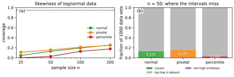
fig_8_s3. Download: PDF · SVG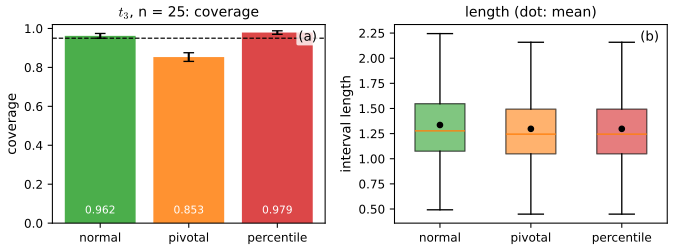
fig_8_s4. Download: PDF · SVG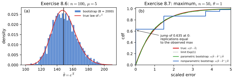
fig_8_s6. Download: PDF · SVGDemonstrations for this chapter
Each demonstration runs in the browser and links back to these notes. The ▶ Demo boxes above open them already set to the case under discussion.
| Demonstration | What you can see | Sections and results |
|---|---|---|
| Coverage of the three bootstrap intervals | For seven statistic and population pairs, the bootstrap histogram and the Normal, pivotal and percentile intervals of any one of \(R\) simulated data sets; the coverage of each method with the side on which it misses; the first 40 intervals. Presets: 1 lognormal skewness, \(n=50\); 2 the same, \(n=200\); 3 exponential mean; 4 scaled IQR of \(t_3\); 5 the uniform maximum. | Section 8.3; Filling the gaps 8.6, 8.8, 8.12; Exercises 8.2, 8.3, 8.7 |
| The jackknife against the bootstrap | For one data set, the centred bootstrap replications, the inflated jackknife values and the true sampling distribution; over \(R\) data sets, the ratio of each estimated standard error to the true one. Presets: 1 median, odd \(n\); 2 median, even \(n\); 3 mean; 4 skewness of the nerve population; 5 ties. | Sections 8.2, 8.5.1; Filling the gaps 8.10, 8.11 |
| How many replications \(B\)? | On the book's data, \(K\) independent bootstrap runs: the running \(\seboot\) and percentile endpoints against \(B\), the ideal values, and the Monte Carlo spread against the \(1/\sqrt B\) formula. Presets: 1 nerve skewness; 2 nerve median; 3 law school correlation; 4 patch ratio; 5 nerve mean. | Sections 8.1, 8.2; Filling the gaps 8.2, 8.4; Examples 8.2, 8.6, 8.7 |
Related demonstrations in the companion courses: bootstrapping Darwin's Zea mays data (Statistical Methods for Modern Biology), the bootstrap of a portfolio allocation and which observations a resample contains (Applied Statistical Learning), bootstrap estimates of prediction error and bootstrap and Bayesian bands (Statistical Learning: Theory and Methods). The Python code that produces every figure of this page is code/ch08_bootstrap.py; see the code index.
References
- Wasserman, L. (2004). All of Statistics: A Concise Course in Statistical Inference. Springer, New York. Chapter 8, pp. 107–118, and Section 9.11. www.stat.cmu.edu/~larry/all-of-statistics.
- Bickel, P. J. and Freedman, D. A. (1981). Some asymptotic theory for the bootstrap. The Annals of Statistics, 9(6), 1196–1217.
- Bickel, P. J., Götze, F. and van Zwet, W. R. (1997). Resampling fewer than \(n\) observations: gains, losses, and remedies for losses. Statistica Sinica, 7(1), 1–31.
- Davison, A. C. and Hinkley, D. V. (1997). Bootstrap Methods and Their Application. Cambridge University Press, Cambridge.
- Efron, B. (1979). Bootstrap methods: another look at the jackknife. The Annals of Statistics, 7(1), 1–26.
- Efron, B. (1982). The Jackknife, the Bootstrap and Other Resampling Plans. SIAM, Philadelphia.
- Efron, B. (1987). Better bootstrap confidence intervals. Journal of the American Statistical Association, 82(397), 171–185.
- Efron, B. and Stein, C. (1981). The jackknife estimate of variance. The Annals of Statistics, 9(3), 586–596.
- Efron, B. and Tibshirani, R. J. (1993). An Introduction to the Bootstrap. Chapman and Hall, New York.
- Ghosh, M., Parr, W. C., Singh, K. and Babu, G. J. (1984). A note on bootstrapping the sample median. The Annals of Statistics, 12(3), 1130–1135.
- Hall, P. (1988). Theoretical comparison of bootstrap confidence intervals. The Annals of Statistics, 16(3), 927–953.
- Hall, P. (1992). The Bootstrap and Edgeworth Expansion. Springer, New York.
- Hall, P. and Martin, M. A. (1988). Exact convergence rate of bootstrap quantile variance estimator. Probability Theory and Related Fields, 80(2), 261–268.
- Quenouille, M. H. (1949). Approximate tests of correlation in time-series. Journal of the Royal Statistical Society, Series B, 11(1), 68–84.
- Scott, D. W., Gotto, A. M., Cole, J. S. and Gorry, G. A. (1978). Plasma lipids as collateral risk factors in coronary artery disease: a study of 371 males with chest pain. Journal of Chronic Diseases, 31, 337–345.
- Shao, J. and Tu, D. (1995). The Jackknife and Bootstrap. Springer, New York.
- Singh, K. (1981). On the asymptotic accuracy of Efron's bootstrap. The Annals of Statistics, 9(6), 1187–1195.
- van der Vaart, A. W. (1998). Asymptotic Statistics. Cambridge University Press, Cambridge.
- van der Vaart, A. W. and Wellner, J. A. (1996). Weak Convergence and Empirical Processes. Springer, New York.
The numerical statements in the text (the plug-in estimates and bootstrap standard errors of the four examples, the exact bootstrap law of the nerve median, the influence-function and jackknife standard errors, the Monte Carlo error formulas, the coverage tables of Exercises 8.2 and 8.3, the jackknife limit laws for the median, the uniform-maximum probabilities, and the corrected formula of Exercise 8.8) were confirmed numerically.