Parametric Inference
When the data are assumed to come from a family of distributions indexed by finitely many numbers, inference reduces to estimating those numbers. This chapter builds the standard toolkit: the method of moments, maximum likelihood and its large-sample theory (consistency, asymptotic normality with the Fisher information, efficiency), the delta method for functions of the estimate, the multiparameter case, the parametric bootstrap, sufficiency and exponential families, and two algorithms for computing the estimate, Newton–Raphson and EM. The book states most of the theory in a few lines and defers the proofs to an appendix or to the literature; these notes prove every result under explicit conditions, show where the conditions bite (Uniform endpoints, superefficiency, misspecification, Newton's saddle points), and repair the slips of the printed text.
Ch. 1 Probability Ch. 2 Random variables Ch. 3 Expectation Ch. 4 Inequalities Ch. 5 Convergence Ch. 6 Models and inference Ch. 7 Estimating the CDF Ch. 8 Bootstrap Ch. 9 Parametric inference Ch. 10 Hypothesis testing Ch. 11 Bayesian inference Ch. 12 Decision theory Ch. 13 Regression Ch. 14 Multivariate models Ch. 15 Independence Ch. 16 Causal inference Ch. 17 Directed graphs Ch. 18 Undirected graphs Ch. 19 Log-linear models Ch. 20 Curve estimation Ch. 21 Orthogonal functions Ch. 22 Classification Ch. 23 Stochastic processes Ch. 24 Simulation
How to read these notes
They follow the book. Sections carry the book's numbers (9.1, 9.2, ..., 9.13.4) and every displayed equation that appears in the book carries the book's own equation number, e.g. \((9.12)\). Numbered items keep the book's numbers (Definition 9.7, Theorem 9.18, Example 9.29). The proofs that the book collects in its appendix (Section 9.13.1) are given where the results are stated.
Filling the gaps. Wherever the book says "it can be shown", quotes a fact without proof, or leaves an argument implicit, an orange Filling the gap box gives the full argument. Proofs and derivations start hidden: open one with its bar, or use the button below.
Figures and demonstrations. Both figures of the chapter (9.1 and 9.2) are reproduced, and eight supplementary figures (9.S1 to 9.S8) illustrate the gaps; all are computed by the Python code. The ▶ Demo boxes open an interactive demonstration already set to the case being discussed.
Main reference
L. Wasserman, All of Statistics: A Concise Course in Statistical Inference, Springer (2004), Chapter 9, pages 119–148 (book website: www.stat.cmu.edu/~larry/all-of-statistics). Section, equation, example and exercise numbers below refer to this book. Further reading is listed in the references.
The explanations, derivations, figures and code are my own; equations are cited by their numbers in the book.
Companion courses
Maximum likelihood, the Fisher information, exponential families and EM appear in every companion course on this site, at other levels and in other words. The overlapping material is:
- First-year notes, Estimation and hypothesis testing (advanced): the method of moments (Section 2.1), maximum likelihood for a proportion and for the Normal model (Theorems 2.2 and 2.3), and the Cramér–Rao bound with a full proof (Theorem 2.4, our Filling the gap 9.12). Its maximum likelihood demo shows the sampling distribution of the MLE against the Cramér–Rao benchmark.
- Statistical Methods for Modern Biology, Chapter 2: likelihood and the MLE (Definition 2.2), the Poisson MLE, its information and precision (Result 2.1, Filling the gap 2.2), the binomial and multinomial MLEs (Results 2.2 and 2.3). Its likelihood for count data demo compares Wald and likelihood-ratio intervals.
- Bayesian and Probabilistic Machine Learning, Chapter 2: maximum likelihood for the multinomial and the Gaussian (Results 2.5 and 2.14), exponential families, their moments, sufficiency and moment matching (Section 2.4, Result 2.23); and Chapter 9, mixtures and EM (Section 9.2, monotonicity in Result 9.15, rate of convergence in Result 9.17).
- Foundations of Deep Learning, Chapter 2: the Gaussian likelihood (Result 2.3) and the Kullback–Leibler divergence, with maximum likelihood as KL minimisation (Result 2.10); Chapter 15, the general EM algorithm and the evidence lower bound (Section 15.3, Result 15.11).
Where a proof there is complete, these notes give the statement and a short argument and link to it. New here: the cost of a nuisance parameter (Filling the gap 9.1), the corrected asymptotic covariance of moment estimators (9.2, 9.3), conditions for consistency and a counterexample (9.6), a complete proof of asymptotic normality (9.9), exact coverage of Wald intervals (9.10), the sample median (9.11), superefficiency (9.13), why the parametric bootstrap works (9.17), misspecification (9.18), and the rate of EM as the fraction of missing information (9.24).
The chapter at a glance
- 9.1 Often only a function \(T(\th)\) matters; the rest of \(\th\) is a nuisance, and it costs information (Filling the gap 9.1).
- 9.2 The method of moments equates \(k\) moments to their sample versions (Definition 9.3); it is consistent and asymptotically Normal (Theorem 9.6, proved in 9.2), but usually not efficient (Figure 9.S1).
- 9.3–9.4 The likelihood and the MLE (Definitions 9.7, 9.8); Bernoulli, Normal and Uniform examples (Figures 9.1, 9.2).
- 9.5–9.6 Consistency through the Kullback–Leibler divergence (Theorem 9.13, 9.5, 9.6); equivariance (Theorem 9.14, 9.7).
- 9.7–9.8 The score and the Fisher information (Theorem 9.17); \(\sqrt n(\hth-\th)\)
\({}\convd\N(0,1/I(\th))\) (Theorem 9.18, proved in 9.9); the Wald interval (Theorem 9.19, 9.10); efficiency, the Cramér–Rao bound and what "optimal" really means (9.11–9.13). - 9.9–9.11 The delta method (Theorem 9.24), the Fisher information matrix and the multiparameter delta method (Theorems 9.27, 9.28), the parametric bootstrap (9.17).
- 9.12 Checking assumptions, and what the MLE estimates when the model is wrong (9.18).
- 9.13 Sufficiency, the factorization theorem, minimal sufficiency and Rao–Blackwell (9.19–9.21); exponential families (9.22); Newton–Raphson and EM (9.23, 9.24).
Notation. \(X_1,\dots,X_n\) iid with density (or probability function) \(f(x;\th)\), \(\th\in\Theta\subset\R^k\); \(\P_\th,\E_\th,\V_\th\) are computed under \(f(\cdot;\th)\). \(\cL_n(\th)=\prod_if(X_i;\th)\), \(\ell_n=\log\cL_n\); \(\hth\) is the MLE; \(\ths\) or simply \(\th\) is the true value. \(\overline X_n\)
Prerequisites. Chapter 5 of the book: the laws of large numbers, the central limit theorem (also for vectors), Slutsky's theorem and the delta method (Theorem 5.5, 5.12, 5.13, 5.15); Jensen's and Gibbs' inequalities (Theorem 4.9, Result 4.10); conditional expectation (Results 3.11, 3.12).
Parametric models
p. 119 A parametric model is a family
\[ \cF=\big\{f(x;\th):\ \th\in\Theta\big\},\qquad\Theta\subset\R^k, \tag{9.1} \]and inference about the distribution reduces to inference about the parameter \(\th=(\th_1,\dots,\th_k)\). The book is candid that we rarely know the data come from such a family, which is why it treats nonparametric methods first (Chapters 7 and 8). Two reasons justify the parametric theory anyway: background knowledge sometimes makes a model reasonable (counts of rare events are often close to Poisson), and the concepts developed here (likelihood, information, efficiency) are the language in which nonparametric methods are later understood. Filling the gap 9.18 says precisely what the MLE estimates when the model is wrong.
9.1 Parameter of Interest
p. 120 Often only a function \(T(\th)\) of the parameter is wanted: the parameter of interest; the remaining coordinates are nuisance parameters. If \(X\sim\N(\mu,\sigma^2)\) and we want \(\mu\), then \(\sigma\) is a nuisance parameter.
Example 9.1 (a blood test). p. 120 With \(X_1,\dots,X_n\)
Here both coordinates of \(\th\) enter \(\tau\). Its MLE is \(1-\Phi((1-\overline X_n)/\hsig)\) by equivariance (Theorem 9.14), and its standard error comes from the multiparameter delta method (Theorem 9.28); Exercise 9.3 does the same computation for a quantile.
Example 9.2 (Gamma lifetimes). p. 120 \(X\sim\Gam(\alpha,\beta)\) has density \(f(x;\alpha,\beta)\)
Filling the gap 9.1: what a nuisance parameter costs p. 120
Write \(\th=(\psi,\lambda)\) with \(\psi\) scalar of interest and \(\lambda\in\R^{k-1}\) a nuisance, and partition the Fisher information matrix of one observation (Section 9.10) accordingly:
\[ I(\th)=\begin{pmatrix}I_{\psi\psi}&I_{\psi\lambda}\\ I_{\lambda\psi}&I_{\lambda\lambda}\end{pmatrix}. \]If \(\lambda\) were known, the MLE of \(\psi\) would have asymptotic variance \(1/(nI_{\psi\psi})\) (Theorem 9.18). With \(\lambda\) unknown it is \((I^{-1})_{\psi\psi}/n\) (Theorem 9.27), and
\[ \frac{1}{(I^{-1})_{\psi\psi}}=I_{\psi\psi}-I_{\psi\lambda}I_{\lambda\lambda}^{-1}I_{\lambda\psi}\ \le\ I_{\psi\psi}, \]with equality if and only if \(I_{\psi\lambda}=0\). The quantity on the left, the efficient information, is what is left of the information about \(\psi\) once the part that could be confused with a change of \(\lambda\) is removed.
Proof and two examples
Let \(M=\begin{pmatrix}a&b^\T\\ b&D\end{pmatrix}\) be positive definite, with \(a\) scalar. Then \(D\) is positive definite (it is a principal submatrix) and \(s=a-b^\T D^{-1}b>0\) (it equals \(v^\T Mv\) for \(v=(1,-D^{-1}b)\ne0\)). The row vector \(r=s^{-1}(1,\,-b^\T D^{-1})\) satisfies \(rM\)
Statistically, \(I_{\psi\psi}-I_{\psi\lambda}I_{\lambda\lambda}^{-1}I_{\lambda\psi}\) is the variance of the residual \(s_\psi-I_{\psi\lambda}I_{\lambda\lambda}^{-1}s_\lambda\) of the \(\psi\)-score after its linear regression on the \(\lambda\)-scores (the scores have covariance matrix \(I\), Filling the gap 9.8).
Normal. For \(\N(\mu,\sigma^2)\), \(I_{\mu\sigma}=0\) (Filling the gap 9.16): not knowing \(\sigma\) costs nothing asymptotically when estimating \(\mu\). Gamma. For \(\Gam(\alpha,\beta)\) the information matrix is \(\begin{pmatrix}\psi'(\alpha)&1/\beta\\1/\beta&\alpha/\beta^2\end{pmatrix}\) (\(\psi'\) the trigamma function), so the efficient information for the shape is \(\psi'(\alpha)-1/\alpha\). At \(\alpha=2\): \(1/\psi'(2)=1.551\) with \(\beta\) known against \(\alpha/(\alpha\psi'(\alpha)-1)\)
9.2 The Method of Moments
pp. 120–121 Method of moments estimators are rarely optimal, but they are easy to compute and make good starting values for iterative methods. For \(1\le j\le k\) define the \(j\)th moment and the \(j\)th sample moment
\[ \alpha_j\equiv\alpha_j(\th)=\E_\th(X^j)=\int x^j\,\d F_\th(x), \tag{9.2} \] \[ \widehat\alpha_j=\frac1n\sum_{i=1}^nX_i^j. \tag{9.3} \]Definition 9.3 (method of moments) p. 121
The method of moments estimator \(\hth\) is the value of \(\th\) that solves the \(k\) equations in \(k\) unknowns
\[ \alpha_1(\hth)=\widehat\alpha_1,\quad\alpha_2(\hth)=\widehat\alpha_2,\quad\dots,\quad\alpha_k(\hth)=\widehat\alpha_k. \tag{9.4} \]Example 9.4. p. 121 For \(\Bern(p)\), \(\alpha_1=p\), so \(\hp=\overline X_n\). Example 9.5. For \(\N(\mu,\sigma^2)\), \(\alpha_1=\mu\) and \(\alpha_2=\sigma^2+\mu^2\) (because \(\V X=\E X^2-(\E X)^2\)); solving gives \(\hmu=\overline X_n\) and \(\hsig^2\)
See also (companion course): the method of moments in the first-year notes, Section 2.1 of Estimation and hypothesis testing (advanced).
Theorem 9.6 (properties of moment estimators; corrected) p. 122
Let \(Y=(X,X^2,\dots,X^k)^\T\), so that \(\alpha(\th)=\E_\th Y\) and \(\widehat\alpha\)
1. With probability tending to 1, (9.4) has a solution \(\hth\) (unique near \(\th\)).
2. \(\hth\convp\th\).
3. \(\sqrt n(\hth-\th)\)
where \(\V_\th(Y)\) is the covariance matrix of \(Y\), with entries \(\alpha_{j+l}(\th)-\alpha_j(\th)\alpha_l(\th)\). The book prints the second-moment matrix \(\E_\th(YY^\T)\) in place of \(\V_\th(Y)\), which gives the wrong answer (Filling the gap 9.3 and the notes on the book); its \(g_j\)
Filling the gap 9.2: proof of Theorem 9.6 p. 122
The theorem is the law of large numbers, the multivariate central limit theorem and the multivariate delta method, glued together by the inverse function theorem.
Proof
Inverse function theorem. Since \(\alpha\) is continuously differentiable with nonsingular Jacobian at \(\th\), there are open sets \(U\ni\th\) and \(W\ni\alpha(\th)\) such that \(\alpha\) maps \(U\) one-to-one onto \(W\) and the inverse \(h=\alpha^{-1}:W\to U\) is continuously differentiable with Jacobian \(Dh(\alpha(\th))\)
1. Each \(\widehat\alpha_j\) is an average of iid variables with finite mean \(\alpha_j(\th)\) (finite because \(\E|X|^j\le1+\E X^{2k}\)), so \(\widehat\alpha\)
2. \(h\) is continuous at \(\alpha(\th)\), so \(h(\widehat\alpha)\)
3. The vectors \(Y_i\) are iid with mean \(\alpha(\th)\) and covariance matrix \(\V_\th(Y)\), finite because \(\E X^{2k}<\infty\). The multivariate central limit theorem (Theorem 5.12) gives \(\sqrt n(\widehat\alpha-\alpha(\th))\)
The centring in the central limit theorem is what makes the covariance, not the raw second moment, appear: \(\sqrt n(\widehat\alpha-\alpha)\) has covariance matrix \(\V_\th(Y)\) exactly, for every \(n\). ∎
Filling the gap 9.3: the Gamma example, and why \(\E(YY^\T)\) cannot be right p. 122, Exercise 9.1
For \(\Gam(\alpha,\beta)\), \(\alpha_1=\alpha\beta\) and \(\alpha_2\)
Theorem 9.6 gives \(\Sigma_{11}\)
Derivation, and a one-line counterexample
With \(\E X^k\)
since \(\Cov(X,X^2)\)
Then \(\Sigma_{11}=g_1\V(Y)g_1^\T\) with \(g_1\)
and the other entries follow in the same way. A simulation with 20 000 samples of size 800 gives \(n\) times the covariance matrix of the estimators as 12.02, \(-5.96\), 3.49 against 12, \(-6\), 3.5 (Figure 9.S1).
Counterexample to \(\E(YY^\T)\). Take \(k=1\) and \(\Bern(p)\): \(Y=X\), \(\alpha(p)=p\), \(G=1\). The truth is \(n\V(\hp)=p(1-p)\), while \(G\,\E(Y^2)G^\T=p\). The two agree only when \(p=0\).
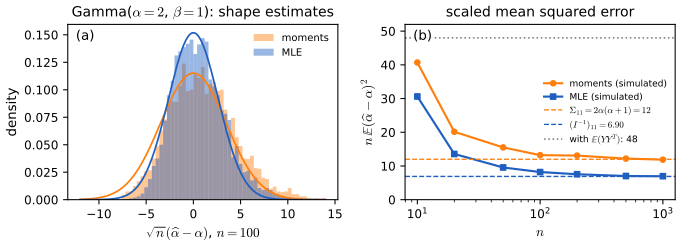
fig_9_s1. Download: PDF · SVGp. 122 The book notes that standard errors from Theorem 9.6 are tedious, and that the bootstrap (Section 9.11) is easier; Figure 9.S1 shows that the moment estimator also loses a large part of the sample.
9.3 Maximum Likelihood
Definition 9.7 (likelihood) p. 122
For \(X_1,\dots,X_n\) iid with density \(f(x;\th)\), the likelihood function and the log-likelihood function are
\[ \cL_n(\th)=\prod_{i=1}^nf(X_i;\th), \tag{9.5} \]and \(\ell_n(\th)=\log\cL_n(\th)\).
The likelihood is the joint density of the data read as a function of \(\th\), \(\cL_n:\Theta\to[0,\infty)\). It is not a density in \(\th\): in general \(\int\cL_n(\th)\,\d\th\ne1\) (and the integral need not even be finite).
Definition 9.8 (maximum likelihood estimator) p. 122
The maximum likelihood estimator (MLE) \(\hth\) is the value of \(\th\) that maximises \(\cL_n(\th)\).
Since \(\log\) is increasing, \(\ell_n\) and \(\cL_n\) have the same maximisers, and \(\ell_n\) (a sum) is usually easier. Remark 9.9. p. 123 Multiplying \(\cL_n\) by a positive constant that does not depend on \(\th\) does not move the maximum, so such constants are dropped freely. The MLE need not exist (the likelihood may be unbounded, Filling the gap 9.4) or be unique (a mixture's likelihood has a twin peak for each relabelling of the components, Figure 9.S8).
Example 9.10 (Bernoulli). p. 123 With \(f(x;p)=p^x(1-p)^{1-x}\), \(x\in\{0,1\}\), and \(S=\sum_iX_i\), \(\cL_n(p)=p^S(1-p)^{n-S}\) and \(\ell_n(p)\)
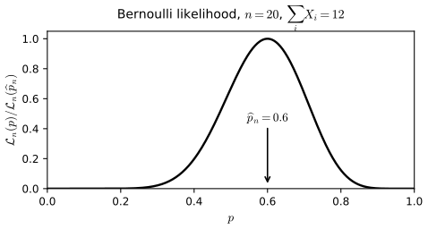
fig_9_1. Download: PDF · SVGSee also (companion courses): the binomial likelihood and its information in Result 2.2 of Statistical Methods for Modern Biology; the MLE for a proportion in Theorem 2.2 of the first-year notes.
Example 9.11 (Normal). pp. 123–124 For \(\N(\mu,\sigma^2)\), dropping constants, and using \(\sum_i(X_i-\mu)^2\)
The likelihood equations give \(\hmu=\overline X_n\) and \(\hsig\)
Filling the gap 9.4: the Normal MLE is the global maximum (and may not exist for \(n=1\)) p. 124
If \(\hsig>0\) (true with probability 1 when \(n\ge2\)), \((\overline X_n,\hsig)\) is the unique global maximiser of \(\ell_n\) on \(\R\times(0,\infty)\). If \(n=1\) the likelihood is unbounded and there is no MLE of \((\mu,\sigma)\).
Proof
For each fixed \(\sigma\), the last term of \(\ell_n\) is \(\le0\) with equality only at \(\mu=\overline X_n\), so \(\ell_n(\mu,\sigma)\)
See also (companion courses): the same computation in Result 2.3 (and Filling the gap 2.5) of Foundations of Deep Learning and in Result 2.14 of Bayesian and Probabilistic Machine Learning (the multivariate case, the book's Theorem 14.5).
Example 9.12 (a hard example: \(\Unif(0,\th)\)). p. 124 Here \(f(x;\th)=1/\th\) for \(0\le x\le\th\) and 0 otherwise. If \(\th<X_i\) for some \(i\), that factor of the likelihood is 0; so \(\cL_n(\th)=0\) for \(\th<X_{(n)}=\max_iX_i\), and \(\cL_n(\th)=\th^{-n}\) for \(\th\ge X_{(n)}\):
\[ \cL_n(\th)=\begin{cases}\th^{-n}&\th\ge X_{(n)},\\0&\th<X_{(n)},\end{cases} \]which is strictly decreasing on \([X_{(n)},\infty)\); hence \(\hth=X_{(n)}\). The likelihood equation \(\ell_n'(\th)=0\) is useless here: the maximum sits at a point where \(\cL_n\) jumps. This model breaks every regularity condition of Sections 9.7 and 9.8 (the support depends on \(\th\)), and its MLE behaves differently: its error is of order \(1/n\), not \(1/\sqrt n\) (Exercise 9.4, Exercise 9.10, and preset 5 of the efficiency demo). The book's errata point out that the density should be written \(\one(x\le\th)/\th\) on a common domain, which is what makes the likelihood argument above correct for every \(\th\).
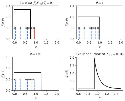
fig_9_2. Download: PDF · SVGp. 124 The MLEs for the multivariate Normal and the multinomial are in the book's Theorems 14.5 and 14.3.
See also (companion courses): the multinomial MLE as observed frequencies in Result 2.5 of Bayesian and Probabilistic Machine Learning and Result 2.3 of Statistical Methods for Modern Biology.
9.4 Properties of Maximum Likelihood Estimators
pp. 124–126 Under regularity conditions (essentially smoothness of \(f(x;\th)\) in \(\th\), with a support that does not depend on \(\th\)), the MLE is:
- consistent: \(\hth\convp\ths\), the true value (Section 9.5);
- equivariant: if \(\hth\) is the MLE of \(\th\), then \(g(\hth)\) is the MLE of \(g(\th)\) (Section 9.6);
- asymptotically Normal: \((\hth-\ths)/\hse\)
\({}\convd\N(0,1)\), with an explicit \(\hse\) (Section 9.7); - asymptotically efficient: roughly, no well-behaved estimator has a smaller variance in large samples (Section 9.8);
- approximately Bayes (the book's Chapter 11).
The precise regularity conditions, which the book does not list, are stated where they are used: Filling the gap 9.6 for consistency, 9.8 and 9.9 for asymptotic normality. In complicated problems (many parameters, irregular supports, misspecified models) these properties can fail; 9.6, 9.13 and 9.18 give examples.
9.5 Consistency of Maximum Likelihood Estimators
p. 126 For densities \(f\) and \(g\), the Kullback–Leibler distance is
\[ D(f,g)=\int f(x)\log\Big(\frac{f(x)}{g(x)}\Big)\d x. \tag{9.6} \]It is not a distance in the formal sense (it is not symmetric, and it can be infinite). Write \(D(\th,\psi)\)
Filling the gap 9.5: \(D(f,g)\ge0\), with equality only when \(f=g\) p. 126
For densities \(f,g\), \(D(f,g)\in[0,\infty]\), and \(D(f,g)=0\) if and only if \(f=g\) almost everywhere. So identifiability in the book's sense is the usual one: \(\th\ne\psi\) implies \(f(\cdot;\th)\ne f(\cdot;\psi)\) on a set of positive measure.
Proof
Let \(A=\{f>0\}\); the integral in (9.6) is over \(A\) (the convention \(0\log0=0\)). If \(g=0\) on a subset of \(A\) of positive \(f\)-probability, \(D=\infty\). Otherwise use \(\log u\le u-1\) for \(u>0\), with equality only at \(u=1\):
\[ -D(f,g)=\int_Af\log\frac gf\ \le\ \int_Af\Big(\frac gf-1\Big)=\int_Ag-1\ \le\ 0. \]Equality throughout forces \(g/f=1\) almost everywhere on \(A\) and \(\int_Ag=1\), i.e. \(g=f\) almost everywhere. (Jensen's inequality for the concave \(\log\) gives the same, Result 4.10.) ∎
Two closed forms used below: \(D(\N(\mu_1,\sigma_1^2),\N(\mu_2,\sigma_2^2))\)
See also (companion courses): Gibbs' inequality and maximum likelihood as KL minimisation, Result 2.10 of Foundations of Deep Learning; Result 4.10 of Chapter 4.
pp. 126–127 Maximising \(\ell_n(\th)\) is the same as maximising \(M_n(\th)\)
which is 0 at \(\ths\) and negative elsewhere. So the maximiser of \(M_n\) should approach the maximiser \(\ths\) of \(M\). Pointwise convergence is not enough to make this rigorous; it must be uniform.
Theorem 9.13 (consistency of the MLE) p. 127; proof p. 135
Suppose
\[ \sup_{\th\in\Theta}|M_n(\th)-M(\th)|\convp0 \tag{9.7} \]and that, for every \(\epsilon>0\),
\[ \sup_{\th:|\th-\ths|\ge\epsilon}M(\th)<M(\ths). \tag{9.8} \]Then the MLE satisfies \(\hth\convp\ths\).
Proof (the book's appendix argument)
\(\hth\) maximises \(M_n\), so \(M_n(\hth)\ge M_n(\ths)\). Hence
\[ 0\le M(\ths)-M(\hth)=\big[M_n(\ths)-M(\hth)\big]+\big[M(\ths)-M_n(\ths)\big]\le\big[M_n(\hth)-M(\hth)\big]+\big[M(\ths)-M_n(\ths)\big]\le2\sup_\th|M_n(\th)-M(\th)|, \]which tends to 0 in probability by (9.7). Fix \(\epsilon>0\). By (9.8) there is \(\delta>0\) with \(M(\th)<M(\ths)-\delta\) whenever \(|\th-\ths|\ge\epsilon\). Therefore \(\P(|\hth-\ths|\ge\epsilon)\)
The same proof works for any \(\tth\) with \(M_n(\tth)\)
Filling the gap 9.6: when do (9.7) and (9.8) hold, and what goes wrong without them p. 127
(a) Compact parameter spaces. Suppose \(\Theta\) is compact, \(\th\mapsto m(x,\th)\)
(b) Concave log-likelihoods. If \(\Theta\) is an open interval and \(\th\mapsto\log f(x;\th)\) is concave for every \(x\) (exponential families in their natural parameter, Section 9.13.3), no compactness or uniformity is needed: identifiability and finiteness of \(M\) suffice for every maximiser of \(\ell_n\) to be consistent.
(c) A counterexample (Neyman and Scott, 1948). Observe pairs \(X_{i1},X_{i2}\)
Proofs
(a) For \(\th\in\Theta\) and \(\rho>0\) put \(u_\rho(x,\th)\)
and symmetrically from below with \(l_j\). The finitely many averages converge almost surely by the strong law (Theorem 5.18), so \(\limsup_n\sup_\th|M_n-M|\)
(b) \(M_n\) is concave and \(M_n(\ths)=0\). Fix \(\epsilon>0\) with \(\ths\pm\epsilon\in\Theta\). By the weak law, \(M_n(\ths\pm\epsilon)\)
(c) For fixed \(\sigma\) the likelihood is maximised by \(\hmu_i=(X_{i1}+X_{i2})/2\); then \(\sum_{j}(X_{ij}-\hmu_i)^2\)
The Cauchy location model of Figure 9.S2 satisfies neither (a) (\(\Theta=\R\)) nor (b) (its log-likelihood is not concave, and has several local maxima for small \(n\)), yet the MLE is consistent: Wald (1949) handles non-compact \(\Theta\) by showing that \(\sup_{|\th|>K}M_n(\th)\) stays below \(M_n(\ths)\) for large \(K\).
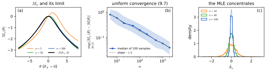
fig_9_s2. Download: PDF · SVG9.6 Equivariance of the MLE
Theorem 9.14 (equivariance) pp. 127–128
Let \(\tau=g(\th)\). If \(\hth\) is the MLE of \(\th\), then \(\htau=g(\hth)\) is the MLE of \(\tau\).
Proof for one-to-one \(g\) (the book's)
Let \(h=g^{-1}\). The likelihood as a function of \(\tau\) is \(\cL^*(\tau)\)
Filling the gap 9.7: equivariance when \(g\) is not one-to-one p. 128
For a general \(g\) (for example \(\tau=\mu^2\), or \(\tau=\mu\) as a function of \(\th=(\mu,\sigma)\)), "the likelihood of \(\tau\)" needs a definition. The standard one is the induced (profile) likelihood \(\cL^*(\tau)\)
Proof
For any \(\tau\) in the range of \(g\), \(\cL^*(\tau)\)
Equivariance is a property of the maximiser, not of the curvature: the Wald interval built on the scale of \(\th\) and the one built on the scale of \(g(\th)\) and mapped back are different intervals (Filling the gap 9.10). The likelihood-ratio interval, a level set of \(\cL\), is equivariant.
Example 9.15. p. 128 For \(\N(\th,1)\), \(\hth=\overline X_n\), and the MLE of \(\tau=e^\th\) is \(e^{\overline X_n}\) (Exercise 9.9 studies its sampling distribution).
9.7 Asymptotic Normality
Definition 9.16 (score and Fisher information) p. 128
The score function and the Fisher information are
\[ s(X;\th)=\frac{\partial\log f(X;\th)}{\partial\th}, \tag{9.9} \] \[ I_n(\th)=\V_\th\Big(\sum_{i=1}^ns(X_i;\th)\Big)=\sum_{i=1}^n\V_\th\big(s(X_i;\th)\big). \tag{9.10} \]For \(n=1\) write \(I(\th)=I_1(\th)\).
Theorem 9.17 and Lemma 9.31 (the information identities) pp. 128, 136
Under the conditions of Filling the gap 9.8, \(\E_\th s(X;\th)=0\) (Lemma 9.31), so \(\V_\th s=\E_\th s^2\); \(I_n(\th)=nI(\th)\); and
\[ I(\th)=-\E_\th\Big(\frac{\partial^2\log f(X;\th)}{\partial\th^2}\Big)=-\int\Big(\frac{\partial^2\log f(x;\th)}{\partial\th^2}\Big)f(x;\th)\,\d x. \tag{9.11} \]Filling the gap 9.8: when the score has mean zero, and when it does not pp. 128, 136
Conditions. (i) The support \(\{x:f(x;\th)>0\}\) does not depend on \(\th\); (ii) \(\th\mapsto f(x;\th)\) is twice differentiable on an open interval; (iii) differentiation under the integral sign is allowed twice: for each \(\th\) there are a neighbourhood \(N\) and integrable functions \(G_1,G_2\) with \(|\partial_\th f(x;\th')|\)
The Uniform model fails. For \(\Unif(0,\th)\), \(\log f=-\log\th\) on the support, so \(s=-1/\th\) and \(\E_\th s=-1/\th\ne0\); worse, \(\E s^2=1/\th^2\) while \(-\E\,\partial^2_\th\log f\)
Proof
Differentiating under the integral. If \(|\partial_\th\phi(x,\th')|\)
Mean zero. \(1=\int_Af(x;\th)\d x\) for all \(\th\), with \(A\) the common support. Differentiating, \(0\)
(9.11). Differentiate \(0=\int_As\,f\,\d x\) once more, using \(\partial_\th f=sf\) (allowed by (iii), since \(\partial_\th(sf)\)
\(I_n=nI\). The \(s(X_i;\th)\) are iid, so the variance of their sum is the sum of the variances.
Uniform. Here the support \([0,\th]\) moves: \(\frac{\d}{\d\th}\int_0^\th\th^{-1}\d x\)
The four models of the Wald interval demo have \(I(p)=1/\{p(1-p)\}\) (Bernoulli), \(1/\lambda\) (Poisson), \(1/\lambda^2\) (Exponential with rate \(\lambda\)) and \(2/\sigma^2\) (Normal scale, mean known); for each, \(\E s=0\) and \(\E s^2=-\E s'=I\) were confirmed by numerical integration.
Theorem 9.18 (asymptotic normality of the MLE) p. 129; proof p. 136
Let \(\se=\sqrt{\V(\hth)}\). Under appropriate regularity conditions (those of Filling the gap 9.9):
1. \(\se\approx\sqrt{1/I_n(\th)}\) and
\[ \frac{\hth-\th}{\se}\convd\N(0,1). \tag{9.12} \]2. With \(\hse=\sqrt{1/I_n(\hth)}\),
\[ \frac{\hth-\th}{\hse}\convd\N(0,1). \tag{9.13} \]Informally, \(\hth\approx\N(\th,\hse^2)\) (the book's errata correct the text after the theorem from \(\se\) to \(\se^2\) in this Normal approximation). Statement 1 is best read with \(\se=1/\sqrt{nI(\th)}\), the asymptotic standard error: the exact variance \(\V(\hth)\) can be infinite for every \(n\) (the MLE of \(\logit p\) is \(\pm\infty\) with positive probability) without affecting the limit (9.12).
Filling the gap 9.9: a complete proof of Theorem 9.18 pp. 136–137
The book's proof expands \(\ell'\) to first order and treats "\(\approx\)" as "\(=\)". Here is the argument with a remainder that is controlled. Conditions (Cramér's): \(\Theta\) an open interval containing the true \(\th_0\); the model identifiable with common support; (R1) \(\th\mapsto\log f(x;\th)\) three times continuously differentiable for each \(x\); (R2) the conditions of Filling the gap 9.8, so \(\E s=0\) and \(I=\E s^2=-\E s'\); (R3) \(0<I(\th_0)<\infty\); (R4) there are \(\delta>0\) and \(K(x)\) with \(\E_{\th_0}K(X)<\infty\) and \(|\partial^3_\th\log f(x;\th)|\)
Proof
On the event \(E_n\)
Rearranging,
\[ \sqrt n(\hth-\th_0)=\frac{n^{-1/2}\ell_n'(\th_0)}{-n^{-1}\ell_n''(\th_0)-\tfrac12(\hth-\th_0)\,n^{-1}\ell_n'''(\tth)}=:\frac{\text{TOP}}{\text{BOTTOM}}. \]TOP. \(\ell_n'(\th_0)\)
BOTTOM. \(-n^{-1}\ell_n''(\th_0)\)
Ratio. \((\text{TOP},\text{BOTTOM})\)
(9.13). If \(I\) is continuous at \(\th_0\), \(I(\hth)\convp I(\th_0)\) (continuous mapping), so \(\sqrt{I(\hth)/I(\th_0)}\)
by Theorem 5.5(e). ∎
Two remarks. The observed information \(-\ell_n''(\hth)/n\) also converges to \(I(\th_0)\) (by the argument for BOTTOM), so it can replace \(I(\hth)\) in \(\hse\); Efron and Hinkley (1978) argue that it is often the better choice. In the four models of the Wald demo the two coincide at the MLE (for example \(-\ell_n''(\hp)\)
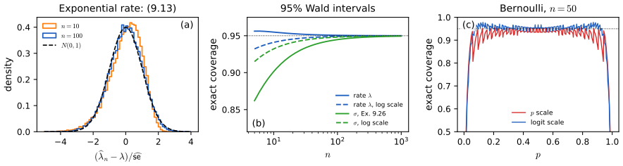
fig_9_s3. Download: PDF · SVGTheorem 9.19 (the Wald interval) p. 129
Let \(C_n\)
Proof
\(\P_\th(\th\in C_n)\)
pp. 129–130 With \(\alpha=0.05\), \(z_{\alpha/2}=1.96\approx2\), and \(\hth\pm2\,\hse\) (9.14) is an approximate 95 percent interval; a poll "accurate to within one point, 95 percent of the time" is reporting such an interval.
Example 9.20 (Bernoulli). p. 130 \(s(X;p)=X/p-(1-X)/(1-p)\), \(-s'(X;p)=X/p^2+(1-X)/(1-p)^2\), so \(I(p)\)
Filling the gap 9.10: how good is the Wald interval, and on which scale? pp. 129–130
Theorem 9.19 is a limit for each fixed \(\th\); it says nothing about a given \(n\). The exact coverage can be computed. For the Bernoulli and Poisson models it is a finite sum over the sufficient statistic; for the Exponential rate and the Normal scale the interval is built from a pivot (a function of data and parameter whose law does not depend on the parameter), and its coverage is a Gamma or chi-square probability that does not depend on \(\th\):
\[ \text{Exponential: }\P\big(n-z\sqrt n\le T\le n+z\sqrt n\big),\ T=\lambda\textstyle\sum_iX_i\sim\Gam(n,1);\qquad\text{Normal }\sigma:\ \P\Big(\frac{n}{(1+c)^2}\le W\le\frac{n}{(1-c)^2}\Big),\ W\sim\chi^2_n,\ c=\frac{z}{\sqrt{2n}}. \]An equally valid interval is built on the scale of \(\psi=g(\th)\) (logit for \(p\), log for \(\lambda\) and \(\sigma\)) by the delta method and mapped back; by equivariance both are centred at the MLE, but they differ. At \(n=10\) the two 95% intervals for the Exponential rate cover with probability 0.955 and 0.941, for the Normal \(\sigma\) of Example 9.26 0.902 (the \(\sigma\) scale) and 0.932 (the log scale); for a Bernoulli \(p=0.2\) and \(n=50\), 0.938 and 0.951. Near the edge of the parameter space both fail: for \(p=0.03\) and \(n=50\) there is no success at all with probability \(0.97^{50}=0.218\), the estimated information is infinite, and the coverages are 0.781 and 0.719.
Derivations
Exponential. \(\widehat\lambda\)
Which scale is better is a property of the model: the log scale wins for the Normal scale parameter (the likelihood of \(\sigma\) is skewed to the right, and so is the log-scale interval), the rate scale for the Exponential at small \(n\) (it is slightly conservative). The likelihood-ratio interval \(\{\th:\ell_n(\hth)-\ell_n(\th)\)
See also (companion courses): the Poisson MLE, information and precision in Filling the gap 2.2 of Statistical Methods for Modern Biology, with its likelihood for count data demo (Wald against likelihood-ratio intervals); Wald intervals for proportions in Theorem 3.9 of the first-year notes.
9.8 Optimality
pp. 130–131 For \(\N(\th,\sigma^2)\) the MLE \(\overline X_n\) satisfies \(\sqrt n(\overline X_n-\th)\)
Filling the gap 9.11: the asymptotic distribution of the sample median p. 131
Let \(X_1,\dots,X_n\) be iid with cdf \(F\) and median \(m\) (\(F(m)=1/2\)), and suppose \(F\) has a density \(f\) that is continuous and positive at \(m\). Then the sample median \(\tth\) satisfies
\[ \sqrt n(\tth-m)\convd\N\Big(0,\frac1{4f(m)^2}\Big). \]For \(\N(\th,\sigma^2)\), \(f(m)=1/(\sigma\sqrt{2\pi})\) and the variance is \(\pi\sigma^2/2\). For the Cauchy location model, \(f(m)=1/\pi\) and the variance is \(\pi^2/4=2.47\), worse than the MLE's \(1/I=2\) (\(\are=8/\pi^2=0.81\)); but the sample mean of Cauchy data is itself Cauchy and not consistent at all. For the Laplace density \(\tfrac12e^{-|x-\th|}\) the median is the MLE.
Proof
Take \(n=2k+1\) odd (for even \(n\) the median lies between \(X_{(k)}\) and \(X_{(k+1)}\), which differ by \(o_P(n^{-1/2})\), and the same limit follows). Fix \(t\) and let \(a_n=m+t/\sqrt n\). The median is \(X_{(k+1)}\), and \(X_{(k+1)}\le a_n\) iff at least \(k+1\) observations are \(\le a_n\). So with \(B_n\)
By differentiability of \(F\) at \(m\), \(p_n\)
Simulation (20 000 samples) gives \(n\V(\text{median})\)
Theorem 9.23 (efficiency of the MLE) p. 131
If \(\hth\) is the MLE and \(\tth\) is any other estimator, then \(\are(\tth,\hth)\le1\).
So the MLE has the smallest asymptotic variance: it is efficient or asymptotically optimal. The book's footnote warns that the truth is "more subtle". Indeed, read literally the theorem is false (Filling the gap 9.13); what is true is that \(1/I(\th)\) is a lower bound in two precise senses: for unbiased estimators at every \(n\) (Cramér–Rao, Filling the gap 9.12), and for every estimator in a local minimax sense (Hájek and Le Cam). The result also assumes the model is right; under misspecification the MLE can be beaten (Filling the gap 9.18). Decision theory (the book's Chapter 12) treats optimality in general.
Filling the gap 9.12: the Cramér–Rao lower bound p. 131
Assume the conditions of Filling the gap 9.8 and \(0<I(\th)<\infty\). Let \(T=T(X_1,\dots,X_n)\) have finite variance and \(\E_\th T=\psi(\th)\) for all \(\th\) in an open interval, and suppose \(\frac{\d}{\d\th}\int T\prod_if(x_i;\th)\,\d x\)
with equality if and only if \(T-\psi(\th)\)
Proof
Let \(S_n=\sum_is(X_i;\th)\), the derivative of \(\log\prod_if(X_i;\th)\); \(\E S_n=0\) and \(\V S_n=nI(\th)\) (Theorem 9.17). Differentiating \(\psi(\th)=\int T\prod f\) gives \(\psi'(\th)\)
Example. For \(\Pois(\lambda)\) and \(\psi=e^{-\lambda}=\P(X=0)\), the bound is \(\lambda e^{-2\lambda}/n\). The unbiased estimator \((1-1/n)^S\) of Filling the gap 9.21 has variance \(e^{-2\lambda}(e^{\lambda/n}-1)\), strictly larger (because \(e^x-1>x\)) but with ratio tending to 1 (Figure 9.S7): the bound is attained only asymptotically.
See also (companion course): the same proof for unbiased estimators of \(\th\), Theorem 2.4 of the first-year notes.
Filling the gap 9.13: superefficiency, and what "efficient" really means p. 131, footnote 3
Hodges' estimator. For \(\N(\th,1)\) let \(T_n=\overline X_n\) if \(|\overline X_n|>n^{-1/4}\) and \(T_n=0\) otherwise. Then \(\sqrt n(T_n-\th)\)
What is true (Le Cam, 1953; Hájek, 1972; see van der Vaart, 1998, Chapter 8). In a regular model: (i) superefficiency is possible only on a set of parameter values of Lebesgue measure zero; (ii) for every estimator sequence, \[ \lim_{c\to\infty}\liminf_n\sup_{|\th-\th_0|\le c/\sqrt n}n\,\E_\th(T_n-\th)^2\ge1/I(\th_0), \] the local asymptotic minimax bound, which the MLE attains; (iii) for estimators whose limit law is locally stable ("regular"), that law is \(\N(0,1/I)\) convolved with another distribution. Hodges' estimator gains at one point by losing badly in a shrinking neighbourhood of it.
Proofs for Hodges' estimator
If \(\th\ne0\): \(\P(T_n\ne\overline X_n)\)
Exact MSE. With \(a=n^{-1/4}\), \(s=1/\sqrt n\) and \(Z=(\overline X_n-\th)/s\), \[ (T_n-\th)^2=(\overline X_n-\th)^2-\{(\overline X_n-\th)^2-\th^2\}\one(|\overline X_n|\le a). \] Using \(\E[Z^2\one(l\le Z\le h)]\)
At \(\th=a\), \(\Phi(h)-\Phi(l)\approx1/2\), so \(n\,\mse\gtrsim\tfrac12n\th^2\)
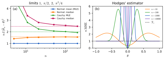
fig_9_s4. Download: PDF · SVG9.9 The Delta Method
pp. 131–132 Let \(\tau=g(\th)\) for a smooth \(g\). By equivariance \(\htau=g(\hth)\) is the MLE of \(\tau\); the delta method gives its distribution.
Theorem 9.24 (the delta method for the MLE) pp. 131–132; outline of proof p. 137
If \(g\) is differentiable and \(g'(\th)\ne0\), then
\[ \frac{\htau-\tau}{\hse(\htau)}\convd\N(0,1), \tag{9.15} \]where \(\htau=g(\hth)\) and
\[ \hse(\htau)=|g'(\hth)|\,\hse(\hth). \tag{9.16} \]Hence, if \(C_n\)
Filling the gap 9.14: completing the outline p. 137
The book's outline linearises \(g\) and invokes Theorem 9.18. The rigorous version needs the conditions of Theorem 9.18 plus continuity of \(g'\) and of \(I\) at \(\th\) (for the estimated standard error).
Proof
By Filling the gap 9.9, \(\sqrt n(\hth-\th)\)
See also: the delta method demo of Chapter 5, which compares the exact law of \(g(\overline X_n)\) with the Normal approximation.
Example 9.25 (log-odds). p. 132 For \(\Bern(p)\) and \(\psi=g(p)=\log\{p/(1-p)\}\), \(\hse(\hp)\)
Example 9.26 (log of a standard deviation). pp. 132–133 For \(\N(\mu,\sigma^2)\) with \(\mu\) known, \(\ell(\sigma)\)
9.10 Multiparameter Models
p. 133 For \(\th=(\th_1,\dots,\th_k)\) with MLE \(\hth\)
and \(J_n(\th)=I_n^{-1}(\th)\). As in one dimension, \(I_n=nI\) with \(I\) the information matrix of one observation, which also equals the covariance matrix of the score vector \(\nabla_\th\log f(X;\th)\).
Theorem 9.27 (asymptotic normality, several parameters) p. 133
Under appropriate regularity conditions, \(\hth-\th\approx\N(0,J_n)\). In particular, with \(\hse_j^2=J_n(j,j)\) (evaluated at \(\hth\)),
\[ \frac{\widehat\theta_j-\th_j}{\hse_j}\convd\N(0,1), \tag{9.19} \]and \(\Cov(\widehat\theta_j,\widehat\theta_k)\)
Theorem 9.28 (the multiparameter delta method) pp. 133–134
Let \(\tau=g(\th_1,\dots,\th_k)\) with gradient \(\nabla g\)
\(\widehat J_n=J_n(\hth)\) and \(\widehat\nabla g\) is \(\nabla g\) evaluated at \(\hth\).
Filling the gap 9.15: proofs of Theorems 9.27 and 9.28 p. 133
Assume the multivariate versions of the conditions of Filling the gap 9.9: \(\Theta\subset\R^k\) open, \(\log f\) three times continuously differentiable in \(\th\) with third derivatives bounded near \(\th_0\) by an integrable \(K(x)\), differentiation under the integral twice (so \(\E\nabla\log f=0\) and \(\Cov(\nabla\log f)\)
Proof
Apply the mean value theorem to each coordinate \(j\) of the gradient along the segment from \(\th_0\) to \(\hth\): \(0\)
by Slutsky's theorem for vectors and the continuity of matrix inversion; \(I^{-1}W\)
Example 9.29 (coefficient of variation). p. 134 For \(\N(\mu,\sigma^2)\) and \(\tau\)
Filling the gap 9.16: the Fisher matrix of \(\N(\mu,\sigma^2)\), and the corrected standard error p. 134, Exercise 9.8
The book prints \(1/\hmu^4\) where \(\hsig^4/\hmu^4\) belongs (listed in the author's errata). The two agree only when \(\hsig=1\). For \(\mu=5\), \(\sigma=2\): \(\sqrt n\,\se=0.325\) against 0.286 from the printed formula, while simulation gives 0.326 at \(n=50\) (Figure 9.S5(b)).
Derivation
\(\log f\)
9.11 The Parametric Bootstrap
pp. 134–135 Standard errors and intervals can also be estimated by the bootstrap, with one change: instead of resampling from the empirical cdf \(\widehat F_n\), simulate \(X_1^*,\dots,X_n^*\) from the fitted model \(f(x;\hth)\), where \(\hth\) may be the MLE or a moment estimator.
Example 9.30. pp. 134–135 For Example 9.29, simulate \(X_1^*,\dots,X_n^*\)
The bootstrap needs no derivatives; the delta method gives a formula.
Filling the gap 9.17: why the parametric bootstrap works, and when the nonparametric one fails pp. 134–135, Exercises 9.9, 9.10
Consistency. Suppose the limit law is locally uniform: whenever \(\th_n\to\th\), the law of \(\sqrt n(\htau-g(\th_n))\) under \(\th_n\) converges to \(\N(0,v(\th))\), with \(v\) continuous (this holds in regular models, for example by the Berry–Esseen bound for smooth functions of means). Then the bootstrap law of \(\sqrt n(\htau^*-\htau)\) given the data converges in probability to \(\N(0,v(\th))\): the bootstrap distribution, its quantiles and (under uniform integrability) \(\hse_{\rm boot}\) are consistent.
Centring. The book centres at \(\htau\); the usual definition centres at \(\overline\tau^*\)
An exact case. For \(\Unif(0,\th)\), \(\hth/\th\) has the Beta(\(n\),1) law whatever \(\th\), and the parametric bootstrap draws \(\th^*=\hth\max_iU_i\), so \(\th^*/\hth\) has the same Beta(\(n\),1) law: the parametric bootstrap reproduces the law of \(\hth/\th\) exactly. The nonparametric bootstrap instead puts mass \(1-(1-1/n)^n\to1-e^{-1}=0.632\) on \(\th^*=\hth\) (Exercise 9.10), while \(n(\th-\hth)\) has a continuous Exponential limit: it is inconsistent here, because the maximum depends on the extreme tail of \(F\), which \(\widehat F_n\) cannot reproduce.
Proof of the consistency statement
Let \(H_n(\th)\) denote the law of \(\sqrt n(\htau-g(\th))\) when the data come from \(\th\); the bootstrap law is \(H_n(\hth)\), a random distribution. Let \(\rho\) be a metric for convergence in distribution (for example the Lévy metric). Suppose \(\rho(H_n(\hth),\N(0,v(\th)))\) did not tend to 0 in probability: then for some \(\epsilon,\eta>0\) and a subsequence, \(\P(\rho(H_n(\hth),\N(0,v))>\epsilon)\)
The Monte Carlo error is separate: given the data, \(\hse_{\rm boot}\) converges as \(B\to\infty\) to the standard deviation of the bootstrap law, by the law of large numbers.
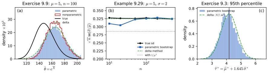
fig_9_s5. Download: PDF · SVGSee also: the nonparametric bootstrap in Chapter 8 of the book; the .632 bootstrap demo of Statistical Learning: Theory and Methods, where the same \(1-(1-1/n)^n\to0.632\) appears as the chance that an observation is in a bootstrap sample.
9.12 Checking Assumptions
p. 135 A parametric assumption should be checked, informally by plots (a clearly bimodal histogram argues against a Normal model; a Normal quantile plot should be roughly straight) or formally by a goodness-of-fit test (the book's Section 10.8). It is also worth knowing what the MLE does when the check fails.
Filling the gap 9.18: what the MLE estimates when the model is wrong pp. 119, 131, 135; Exercise 9.6(e)
Let \(X_1,\dots,X_n\) be iid from a density \(g\) that need not belong to \(\{f(\cdot;\th)\}\). Under the conditions of Theorem 9.13 with \(M(\th)=\E_g\log f(X;\th)\), the MLE converges to the KL projection
\[ \th_g=\argmax_\th\E_g\log f(X;\th)=\arg\min_\th D\big(g,f(\cdot;\th)\big), \]and under the conditions of Theorem 9.18, \(\sqrt n(\hth-\th_g)\)
Examples. (i) A Poisson model fitted to overdispersed counts: \(\th_g=\E_gX\) (the MLE \(\overline X_n\) is still consistent for the mean), \(J=1/\lambda\), \(K=\V_g(X)/\lambda^2\), so the sandwich is \(\V_g(X)\) while the model-based variance is \(\lambda\): the Wald interval is too narrow by the factor \(\sqrt{\lambda/\V_gX}\). (ii) Exercise 9.6(e): with the \(\N(\th,1)\) model, \(\th_g=\E_gX\), so \(\Phi(\overline X_n)\)
Proof sketch
\(M_n(\th)\)
9.13 Appendix
9.13.1 Proofs
pp. 135–137 The book's appendix proves Theorem 9.13, Lemma 9.31, Theorem 9.18 and outlines Theorem 9.24. These notes give those proofs where the results are stated, with the details completed: Theorem 9.13 (and Filling the gap 9.6), Lemma 9.31 in Filling the gap 9.8, Theorem 9.18 in Filling the gap 9.9, Theorem 9.24 in Filling the gap 9.14. Two small points of the book's proof of Theorem 9.18: it divides by \(\ell''\) without checking that the denominator stays away from 0 (BOTTOM \(\convp I>0\) does that), and it uses Theorem 5.5(e) for a ratio, which needs the continuous mapping \(v\mapsto1/v\) at \(I\ne0\) first.
9.13.2 Sufficiency
p. 137 A statistic is a function \(T(X^n)\) of the data \(X^n=(X_1,\dots,X_n)\) (the book's errata add this definition of \(X^n\)); a sufficient statistic contains all the information in the data about \(\th\).
Definition 9.32 (sufficiency through the likelihood) p. 137
Write \(x^n\leftrightarrow y^n\) if \(f(x^n;\th)=c\,f(y^n;\th)\) for some constant \(c\) that may depend on \(x^n\) and \(y^n\) but not on \(\th\). A statistic \(T\) is sufficient if \(T(x^n)=T(y^n)\) implies \(x^n\leftrightarrow y^n\). (The book prints "\(T(x^n)\leftrightarrow T(y^n)\)"; the errata correct it to "=".)
If \(x^n\leftrightarrow y^n\), the two data sets give likelihood functions of the same shape, hence the same MLE and the same likelihood-based inferences; so \(T\) is sufficient when the likelihood (up to a constant) can be computed from \(T\) alone.
Example 9.33. p. 137 For \(\Bern(p)\), \(\cL(p)=p^S(1-p)^{n-S}\), so \(S=\sum_iX_i\) is sufficient. Example 9.34. p. 138 For \(\N(\mu,\sigma^2)\) (the book writes \(\N(\mu,\sigma)\)), \[ f(X^n;\mu,\sigma)=(\sigma\sqrt{2\pi})^{-n}\exp\{-n\hsig^2/(2\sigma^2)\}\exp\{-n(\overline X_n-\mu)^2/(2\sigma^2)\} \] depends on the data only through \(T=(\overline X_n,\hsig)\), which is therefore sufficient; so is \((17\,\overline X_n,\hsig)\), or the whole sample \(T_1=(X_1,\dots,X_n)\), or \(T_4\)
Definition 9.35 (minimal sufficiency) p. 138
A statistic \(T\) is minimal sufficient if (i) it is sufficient and (ii) it is a function of every other sufficient statistic.
Theorem 9.36 p. 138
\(T\) is minimal sufficient if \(T(x^n)=T(y^n)\) holds if and only if \(x^n\leftrightarrow y^n\).
Filling the gap 9.20: proof of Theorem 9.36, and the Normal case p. 138
Proof
Sufficiency. The "only if" half of the hypothesis, \(T(x^n)\)
Minimality. Let \(U\) be any sufficient statistic. If \(U(x^n)=U(y^n)\) then \(x^n\leftrightarrow y^n\) (sufficiency of \(U\)), hence \(T(x^n)=T(y^n)\) (the "if" half). So \(T\) is constant on every level set of \(U\), and \(\varphi(u)=T(x^n)\) for any \(x^n\) with \(U(x^n)=u\) is a well-defined function with \(T=\varphi(U)\). ∎
Example 9.38. For \(\N(\mu,\sigma^2)\),
\[ \frac{f(x^n;\mu,\sigma)}{f(y^n;\mu,\sigma)}=\exp\Big\{-\frac{1}{2\sigma^2}\Big[\sum_ix_i^2-\sum_iy_i^2\Big]+\frac{\mu}{\sigma^2}\Big[\sum_ix_i-\sum_iy_i\Big]\Big\}, \]which is free of \((\mu,\sigma)\) iff both brackets vanish, i.e. iff \((\overline x,\hsig_x)\)
Example 9.37 (partitions). pp. 138–139 For two Bernoulli trials, \(V=X_1\), \(T=X_1+X_2\) and \(U=(T,X_1)\) induce the partitions
| statistic | partition of \(\{00,01,10,11\}\) | sufficient? | minimal? |
|---|---|---|---|
| \(V=X_1\) | \(\{00,01\},\{10,11\}\) | no | no |
| \(T=X_1+X_2\) | \(\{00\},\{01,10\},\{11\}\) | yes | yes |
| \(U=(T,X_1)\) | \(\{00\},\{01\},\{10\},\{11\}\) | yes | no |
The likelihood-equivalence classes of \(\leftrightarrow\) are exactly the cells of \(T\) (\(01\leftrightarrow10\) since both have likelihood \(p(1-p)\)), so \(T\) is minimal by Theorem 9.36; \(U\) splits a class; \(17\,T\) induces the same partition as \(T\) and is also minimal sufficient. Sufficiency is a property of the partition, not of the labels.
p. 139 The usual definition is different: \(T\) is sufficient if the conditional distribution of \(X^n\) given \(T(X^n)=t\) does not depend on \(\th\). Example 9.39. For two flips and \(T=X_1+X_2\): given \(T=0\) the data are \((0,0)\); given \(T=2\), \((1,1)\); given \(T=1\), \((0,1)\) and \((1,0)\) each with probability \(p(1-p)/\{2p(1-p)\}=1/2\). None depends on \(p\) (the errata replace a stray \(\th\) by \(p\) here).
Theorem 9.40 (factorization) p. 140
\(T\) is sufficient if and only if there are functions \(g(t,\th)\) and \(h(x^n)\) such that \(f(x^n;\th)\)
Example 9.41. p. 140 For two flips, \(f(x_1,x_2;\th)\)
Filling the gap 9.19: the two definitions of sufficiency agree, and the factorization theorem pp. 137, 139–140
Call (A) Definition 9.32, (B) the conditional definition and (C) the factorization. Then (A) \(\Leftrightarrow\) (C) for densities in general (on the points that have positive density for some \(\th\); the errata's convention that all \(f(\cdot;\th)\) live on a common domain, e.g. \(\one(x\le\th)/\th\) for the Uniform, is what makes this work), and (B) \(\Leftrightarrow\) (C) for discrete data. So all three are equivalent for discrete models, and Theorem 9.40 holds with either definition.
Proof
(C) \(\Rightarrow\) (A). If \(T(x)=T(y)\) and \(h(y)>0\), then \(f(x;\th)\)
(A) \(\Rightarrow\) (C). For each value \(t\) of \(T\) choose one point \(x_t\) with \(T(x_t)=t\). For any \(x\), \(T(x)=T(x_{T(x)})\), so by (A) \(f(x;\th)=c(x)f(x_{T(x)};\th)\) with \(c(x)\) free of \(\th\). Put \(g(t,\th)=f(x_t;\th)\) and \(h(x)=c(x)\).
(C) \(\Rightarrow\) (B), discrete. If \(\P_\th(T=t)>0\) and \(T(x)=t\),
\[ \P_\th(X^n=x\given T=t)=\frac{f(x;\th)}{\sum_{y:T(y)=t}f(y;\th)}=\frac{g(t,\th)h(x)}{g(t,\th)\sum_{y:T(y)=t}h(y)}=\frac{h(x)}{\sum_{y:T(y)=t}h(y)}, \]free of \(\th\) (and the conditional probability is 0 when \(T(x)\ne t\)).
(B) \(\Rightarrow\) (C), discrete. \(f(x;\th)\)
For continuous data the conditional distribution given \(T=t\) lives on a lower-dimensional set, and (B) \(\Leftrightarrow\) (C) needs measure theory (Halmos and Savage, 1949); the factorization is what one uses in practice.
p. 140 Let \(R(\th,\hth)\)
Theorem 9.42 (Rao–Blackwell) p. 140
Let \(\hth\) be an estimator, \(T\) a sufficient statistic, and \(\tth=\E(\hth\given T)\). Then \(R(\th,\tth)\le R(\th,\hth)\) for every \(\th\).
Filling the gap 9.21: proof of Rao–Blackwell, and an example where it matters p. 140
The improvement is strict unless \(\hth\) is already a function of \(T\). Example 9.43 with \(n\) flips: \(\E(X_1\given T)=T/n\). Poisson zeros: for \(\Pois(\lambda)\) data and \(\psi=e^{-\lambda}=\P(X=0)\), the naive unbiased estimator \(\one(X_1=0)\) has variance \(e^{-\lambda}(1-e^{-\lambda})\); its Rao–Blackwellisation is \(\E(\one(X_1=0)\given S)\)
Proof
\(\tth\) is an estimator. By sufficiency (in the conditional form (B) of Filling the gap 9.19) the conditional law of the data given \(T\) is free of \(\th\), so \(\E(\hth\given T)\) can be computed without knowing \(\th\).
Same bias. \(\E_\th\tth\)
Smaller variance. By the law of total variance (Result 3.12), \(\V_\th\hth\)
Example 9.43. By symmetry \(\E(X_i\given T)\) is the same for every \(i\), and the \(n\) of them sum to \(\E(T\given T)=T\); so each is \(T/n\).
Poisson. \(\P(X_1=k\given S=s)\)
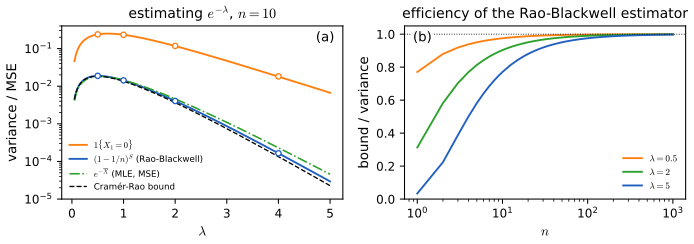
fig_9_s7. Download: PDF · SVG9.13.3 Exponential Families
p. 140 \(\{f(x;\th):\th\in\Theta\}\) is a one-parameter exponential family if there are functions \(\eta(\th)\), \(B(\th)\), \(T(x)\) and \(h(x)\) with
\[ f(x;\th)=h(x)\,e^{\eta(\th)T(x)-B(\th)}. \]By the factorization theorem \(T(X)\) is sufficient, the natural sufficient statistic; for an iid sample, \(f(x^n;\th)\)
Example 9.44. p. 141 \(\Pois(\th)\): \(f=\frac1{x!}e^{x\log\th-\th}\), so \(\eta=\log\th\), \(B=\th\), \(T(x)=x\), \(h=1/x!\). Example 9.45. \(\Bin(n,\th)\): \(f\)
p. 141 In the natural parametrisation, \(f(x;\eta)\)
Example 9.46 (not an exponential family). p. 141 For \(\Unif(0,\th)\), \(f(x^n;\th)\)
Theorem 9.47 (moments of the natural statistic) p. 142
If \(X\) has density \(h(x)e^{\eta T(x)-A(\eta)}\) with \(\eta\) interior to the natural parameter space \(\{\eta:\int he^{\eta T}\)
Example 9.48. p. 142 \(\N(\mu,\sigma^2)\) is a two-parameter exponential family: \[ f=\exp\{\frac{\mu}{\sigma^2}x-\frac{x^2}{2\sigma^2}-\frac12(\frac{\mu^2}{\sigma^2}+\log(2\pi\sigma^2))\}, \] with \(\eta_1=\mu/\sigma^2\), \(T_1=x\), \(\eta_2=-1/(2\sigma^2)\), \(T_2=x^2\), \(h=1\); so \((\sum_iX_i,\sum_iX_i^2)\) is sufficient for an iid sample.
Filling the gap 9.22: proof of Theorem 9.47, and the MLE in an exponential family pp. 141–142
Beyond the moments: \(A\) is convex; the moment generating function of \(T\) is \(\E e^{uT}\)
Proof
\(e^{A(\eta)}\)
Two checks: for the Poisson, \(A(\eta)=e^\eta\), so \(\E X=\V X=e^\eta=\lambda\); for the Bernoulli, \(A(\eta)=\log(1+e^\eta)\), \(A'=e^\eta/(1+e^\eta)=p\), \(A''=p(1-p)\).
See also (companion course): the same results, with conjugate priors, in Result 2.23 of Bayesian and Probabilistic Machine Learning.
9.13.4 Computing Maximum Likelihood Estimates
pp. 142–143 When the MLE has no closed form it is computed iteratively, producing \(\th^0,\th^1,\dots\) that under good conditions converge to \(\hth\). A good starting value helps, and the method of moments often provides one (as for the Gamma shape in Figure 9.S1).
Newton–Raphson p. 143
Expanding the score around the current value, \(0\)
with \(\ell'\) the gradient and \(H\) the Hessian of the log-likelihood at \(\th^j\). Each step jumps to the top of the second-order Taylor approximation of \(\ell\) at \(\th^j\).
Filling the gap 9.23: Newton–Raphson converges quadratically near a root, and may fail away from one p. 143
Let \(F=\ell'\) be twice continuously differentiable near a root \(\hth\) with \(F'(\hth)=\ell''(\hth)\ne0\). There is \(\delta>0\) such that, from any start within \(\delta\) of \(\hth\), the iterates stay within \(\delta\) and
\[ |\th^{j+1}-\hth|\le K|\th^j-\hth|^2,\qquad K=\frac{\sup|F''|}{2\inf|F'|}\ \ \text{(over the interval)}, \]so the number of correct digits roughly doubles at each step. Far from the root nothing is guaranteed: Newton's method solves \(\ell'=0\) and cannot tell a maximum from a minimum or a saddle point; it can overshoot, diverge, or stop where the Hessian is singular. In Figure 9.S8 it converges in 5 steps from one start and to a saddle point from another. Practical versions use the expected information (Fisher scoring, \(\th^{j+1}\)
Proof
Taylor's theorem at \(\th^j\): \(0\)
Choose \(\delta\) so that \(F'\) does not vanish on \([\hth-\delta,\hth+\delta]\) (continuity) and \(K\delta<1\). If \(|\th^j-\hth|\le\delta\) then \(|\th^{j+1}-\hth|\)
The EM algorithm. pp. 143–144 Suppose the density \(f(y;\th)\) of the observed data \(Y\) is hard to maximise, but \(f(y;\th)\)
Example 9.49 (mixture of Normals). pp. 143–144 \(f(y;\th)\)
The EM algorithm p. 144
(0) Pick a starting value \(\th^0\). For \(j=0,1,2,\dots\) repeat:
(1) E-step: compute
\[ J(\th\given\th^j)=\E_{\th^j}\Big(\log\frac{f(Y^n,Z^n;\th)}{f(Y^n,Z^n;\th^j)}\ \Big|\ Y^n=y^n\Big), \]the expectation over the missing \(Z^n\) with \(\th^j\) and the observed data fixed (the book writes \(\th^i\) for \(\th^j\); listed in the author's errata).
(2) M-step: let \(\th^{j+1}\) maximise \(J(\th\given\th^j)\) over \(\th\).
Filling the gap 9.24: EM never decreases the likelihood (corrected proof), Example 9.50 in full, and the rate of EM pp. 144–146
(a) Monotonicity. Let \(k(z\given y;\th)\)
with equality at \(\th=\th^j\). Since \(J(\th^{j+1}\given\th^j)\)
(b) Fixed points are stationary points: if \(\th^j\to\th^\infty\) in the interior and everything is smooth, \(\nabla\ell(\th^\infty)=0\) (Wu, 1983). They need not be maxima: started on the diagonal \(\mu_0=\mu_1\), EM for Example 9.50 stays there forever, because all responsibilities equal 1/2.
(c) Example 9.50 (two Normals with \(p=1/2\), \(\sigma_0=\sigma_1=1\), unknown \(\mu_0,\mu_1\)). With \(\tau_i\)
where \(C_j\) does not depend on \(\th\) (the book drops it and the squares; both listed in the author's errata), and the M-step gives the responsibility-weighted means \(\mu_1^{j+1}\)
(d) The rate. Near the MLE, EM is a linear contraction: \(\th^{j+1}-\hth\)
Proofs
(a) For every \(z\), \(\log f(y;\th)\)
and \(D\ge0\) by Filling the gap 9.5.
(b) \(\th\mapsto D(k_{\th^j},k_\th)\) is minimised (equal to 0) at \(\th=\th^j\), so its gradient vanishes there and \(\nabla_\th J(\th\given\th^j)|_{\th=\th^j}\)
(c) \(f(y,z;\th)\)
(d) In one dimension, let \(M(\th)\) be the EM map: \(\partial_1J(M(\th)\given\th)\)
See also (companion courses): EM for Gaussian mixtures and its monotonicity in Result 9.15 of Bayesian and Probabilistic Machine Learning, with the evidence-lower-bound view in Result 15.11 of Foundations of Deep Learning.
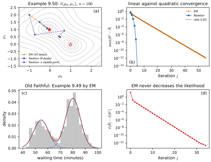
faithful.dat); the fit agrees with scikit-learn's to six digits of the log-likelihood. (d) \(\ell(\hth)-\ell(\th^j)\) for (c): EM never decreases the likelihood. Not a figure of the book. Code: ch09_parametric_inference.py, fig_9_s8. Download: PDF · SVGNotes on the book
Seventeen entries of the author's two errata lists (for the first and the second printing, on the book's website) concern Chapter 9; they are collected in the last box. Four more points are mine, each with the evidence. None changes a main conclusion of the chapter, but the one in Theorem 9.6 changes every standard error computed from it.
Page 122, Theorem 9.6: the covariance of the moment estimator uses \(\E_\th(YY^\T)\) where \(\V_\th(Y)\) belongs
The theorem prints \(\Sigma=g\,\E_\th(YY^\T)g^\T\). The asymptotic covariance of \(\sqrt n(\widehat\alpha-\alpha)\) is the covariance matrix of \(Y=(X,\dots,X^k)\), not its second-moment matrix (Filling the gap 9.2). Evidence: for \(\Bern(p)\) with \(k=1\) the printed formula gives \(p\) instead of \(p(1-p)\); for the Gamma shape at \(\alpha=2\) it gives 48 where the truth, confirmed by simulation (Figure 9.S1), is 12. The description "\(g_j\)
Page 144, Example 9.49: which component has probability \(p\)
The density is \((1-p)\phi(y;\mu_0,\sigma_0)\)
Page 145, the EM monotonicity proof: the Kullback–Leibler term is between conditional densities of the missing data
The proof defines \(f_j=f(y^n;\th^j)\) and \(f_{j+1}=f(y^n;\th^{j+1})\) and writes the remainder as \(K(f_j,f_{j+1})\). The quantity that appears, \[ -\E_{\th^j}[\log\{f(Z^n\given Y^n;\th^{j+1})/f(Z^n\given Y^n;\th^j)\}\given y^n], \] is the divergence between the conditional laws of \(Z^n\) given \(Y^n=y^n\) under \(\th^j\) and \(\th^{j+1}\) (Filling the gap 9.24); the marginal densities of the observed data are fixed numbers here, and a "KL distance" between two numbers is not defined. Not in the errata lists (the errata correct only the missing log on the same display and the \(\th^i\) typos).
Page 141, Example 9.46: the reason the Uniform is not an exponential family
The book argues "since \(T(X^n)\ne\sum_iT(X_i)\), this cannot be an exponential family". The existence of a sufficient statistic that is not a sum does not exclude a representation in which another one is; the conclusion holds because the support of an exponential family, \(\{h>0\}\), cannot depend on \(\th\), while that of \(\Unif(0,\th)\) does. Also in this section: Example 9.50 says "\(\sigma_1=\sigma_2=1\)" for the components it calls 0 and 1, and writes \(f(y^n\given Z_i=1;\th^j)\) where \(f(y_i\given Z_i=1;\th^j)\) is meant; Example 9.34 writes \(\N(\mu,\sigma)\) for \(\N(\mu,\sigma^2)\); and \(2/\pi=0.6366\) is rounded to ".63" in Section 9.8. None of these is in the errata lists.
Slips listed in the author's errata
- p. 122: "treat it is a function" should read "treat it as a function".
- p. 126, last line: "the the" should be "the".
- p. 129, first line after Theorem 9.18: the Normal approximation is \(\N(\th,\hse^2)\), not \(\N(\th,\hse)\).
- p. 134, Example 9.29: the term \(1/\hmu^4\) should be \(\hsig^4/\hmu^4\) (Filling the gap 9.16; the two differ unless \(\hsig=1\), Figure 9.S5(b)).
- p. 134, Example 9.30: the first simulated variable is \(X_1^*\), not \(X_1\).
- p. 137, Section 9.13.2: \(X^n\) means \((X_1,\dots,X_n)\); all densities are defined on a common domain (so the Uniform density is written \(\one(x\le\th)/\th\)); and in Definition 9.32, "\(T(x^n)\leftrightarrow T(y^n)\)" should be "\(T(x^n)=T(y^n)\)".
- p. 139, Example 9.39, last line: \(\th\) should be \(p\).
- p. 141, Example 9.45: \(B(\th)=-n\log(\th)\) should be \(-n\log(1-\th)\) (with the printed \(B\) the binomial probabilities sum to 0.013 for \(n=7\), \(\th=0.35\), instead of 1).
- p. 141, three lines before Example 9.46: one factor \(h_n(x^n)\) too many.
- p. 144: in the E-step, \(\th^i\) should be \(\th^j\); and the last line should begin with a log (it is \(\log\{\cL(\th^{j+1})/\cL(\th^j)\}\)).
- p. 145: \(\th^i\) should be \(\th^j\) near the end of the page; \((y_i-\mu_0)\) and \((y_i-\mu_1)\) should be squared; and a constant term has been dropped from \(J\) (Filling the gap 9.24(c)).
- p. 146, line 1: "\(\mu_1\) and \(\mu_2\)" should be "\(\mu_0\) and \(\mu_1\)".
9.14 Exercises
All ten exercises of Chapter 9 (Wasserman, 2004, pp. 146–148), restated in my own words, with complete solutions (hidden). Numerical answers come from the chapter code (ex93, ex97, ex99, ex910).
Exercise 9.1. For \(X_1,\dots,X_n\)
\({}\sim\Gam(\alpha,\beta)\), find the method of moments estimators of \(\alpha\) and \(\beta\). Solution
\(\E X=\alpha\beta\) and \(\V X=\alpha\beta^2\), so \(\E X^2\)
\({}=\alpha\beta^2+\alpha^2\beta^2\). Equating \(\alpha\beta=\overline X_n\) and \(\alpha\beta^2+\alpha^2\beta^2\) \({}=n^{-1}\sum_iX_i^2\) gives \(\alpha\beta^2=\hsig^2\) (subtract the square of the first equation), so \(\widehat\beta\) \({}=\hsig^2/\overline X_n\) and \(\widehat\alpha\) \({}\) \({}=\overline X_n/\widehat\beta\) \({}=\overline X_n^2/\hsig^2\), where \(\hsig^2\) \({}=n^{-1}\sum_i(X_i-\overline X_n)^2\). Their asymptotic covariance and their efficiency relative to the MLE are in Filling the gap 9.3. Exercise 9.2. Let \(X_1,\dots,X_n\sim\Unif(a,b)\) with \(a<b\) unknown. (a) Find the moment estimators of \(a\) and \(b\). (b) Find the MLEs. (c) For \(\tau=\int x\,\d F(x)\), find the MLE \(\htau\). (d) With \(a=1\), \(b=3\), \(n=10\), find the MSE of \(\htau\) by simulation and the MSE of the plug-in estimator \(\tilde\tau=\overline X_n\) exactly, and compare.
Solution
(a) \(\E X=(a+b)/2\) and \(\V X=(b-a)^2/12\). Solving \((a+b)/2=\overline X_n\), \((b-a)^2/12=\hsig^2\) gives \(\widehat a\)
\({}=\overline X_n-\sqrt3\,\hsig\), \(\widehat b\) \({}=\overline X_n+\sqrt3\,\hsig\). (b) \(\cL(a,b)=(b-a)^{-n}\) if \(a\le X_{(1)}\) and \(X_{(n)}\le b\), and 0 otherwise. It increases as \(b-a\) shrinks, so it is maximised by the smallest admissible interval: \(\widehat a=X_{(1)}\), \(\widehat b=X_{(n)}\).
(c) \(\tau=(a+b)/2\), so by equivariance \(\htau=(X_{(1)}+X_{(n)})/2\), the midrange.
(d) For \(\Unif(0,1)\), \(\V X_{(1)}\)
\({}=\V X_{(n)}\) \({}=n/\{(n+1)^2(n+2)\}\) and \(\Cov(X_{(1)},X_{(n)})\) \({}=1/\{(n+1)^2(n+2)\}\), so the midrange is unbiased (by symmetry) with variance \(\tfrac14\cdot\frac{2n+2}{(n+1)^2(n+2)}\) \({}=\frac1{2(n+1)(n+2)}\); on \([a,b]\) multiply by \((b-a)^2\). With \(b-a=2\), \(n=10\): \(\mse(\htau)=4/264=0.01515\), and a simulation with 200 000 samples gives 0.01513. The plug-in \(\overline X_n\) has \(\mse\) \({}=(b-a)^2/(12n)\) \({}=1/30\) \({}=0.0333\). The MLE is more than twice as accurate; its MSE is of order \(1/n^2\) against \(1/n\), because the endpoints of a uniform are located to within \(O(1/n)\). Exercise 9.3. Let \(X_1,\dots,X_n\)
\({}\sim\N(\mu,\sigma^2)\) and let \(\tau\) be the 0.95 quantile, \(\P(X<\tau)=0.95\). (a) Find the MLE of \(\tau\). (b) Give an approximate \(1-\alpha\) confidence interval. (c) For the 25 observations printed in the book, compute \(\htau\) and its standard error by the delta method and by the parametric bootstrap. Solution
(a) \(\tau=\mu+z\sigma\) with \(z=\Phi^{-1}(0.95)=1.645\), so \(\htau\)
\({}=\overline X_n+1.645\,\hsig\) by equivariance. (b) With \(\nabla g=(1,z)^\T\) and \(J_n\)
\({}=n^{-1}\mathrm{diag}(\sigma^2,\sigma^2/2)\) (Filling the gap 9.16), \(\hse(\htau)\) \({}=\hsig\sqrt{(1+z^2/2)/n}\) and the interval is \(\htau\pm z_{\alpha/2}\hse(\htau)\) (Theorem 9.28). (c) \(n=25\), \(\overline X_n=1.191\), \(\hsig=1.818\), so \(\htau=4.180\); \(\hse\)
\({}=1.818\sqrt{(1+1.353)/25}\) \({}=0.558\), and a 95% interval is \(4.18\pm1.09=(3.09,\,5.27)\). The parametric bootstrap (10 000 samples of size 25 from \(\N(1.191,1.818^2)\)) gives \(\hse_{\rm boot}=0.556\), and its distribution is close to the delta-method Normal (Figure 9.S5(c)). Exercise 9.4. For \(X_1,\dots,X_n\)
\({}\sim\Unif(0,\th)\), show that the MLE is consistent. Solution
\(\hth=Y=X_{(n)}\le\th\). For \(0<\epsilon<\th\), \(\P(|\hth-\th|>\epsilon)\)
\({}=\P(Y<\th-\epsilon)\) \({}\) \({}=\prod_i\P(X_i<\th-\epsilon)\) \({}=(1-\epsilon/\th)^n\) \({}\to0\) (for \(\epsilon\ge\th\) the probability is 0). So \(\hth\convp\th\). Moreover \(\P(n(\th-\hth)>t)\) \({}=(1-t/(n\th))^n\) \({}\to e^{-t/\th}\): the error is of order \(1/n\), with an Exponential limit, not of order \(1/\sqrt n\) with a Normal one. Exercise 9.5. For \(X_1,\dots,X_n\)
\({}\sim\Pois(\lambda)\), find the method of moments estimator, the MLE and the Fisher information \(I(\lambda)\). Solution
\(\E X=\lambda\), so the moment estimator is \(\overline X_n\). \(\ell_n(\lambda)\)
\({}\) \({}=\sum_iX_i\log\lambda-n\lambda\) \({}+\text{const}\) has \(\ell_n'=\sum_iX_i/\lambda-n\), zero at \(\widehat\lambda\) \({}=\overline X_n\), and \(\ell_n''\) \({}=-\sum_iX_i/\lambda^2\) \({}<0\) (if some \(X_i>0\); if all are 0 the maximum is at the boundary \(\widehat\lambda=0\)): the MLE is also \(\overline X_n\). With \(s=X/\lambda-1\) and \(s'=-X/\lambda^2\), \(I(\lambda)\) \({}=\E(X/\lambda^2)\) \({}=1/\lambda\) (equivalently \(\V s\) \({}=\V X/\lambda^2\) \({}=1/\lambda\)). Exercise 9.6. Let \(X_1,\dots,X_n\sim\N(\th,1)\), \(Y_i=\one(X_i>0)\) and \(\psi=\P(Y_1=1)\). (a) Find the MLE \(\hpsi\). (b) Give an approximate 95% interval for \(\psi\). (c) Show that \(\tilde\psi=n^{-1}\sum_iY_i\) is consistent. (d) Find \(\are(\tilde\psi,\hpsi)\). (e) If the data are not Normal, show that \(\hpsi\) is not consistent, and find its limit.
Solution
(a) \(\psi=\P(X>0)=\Phi(\th)\), so \(\hpsi=\Phi(\overline X_n)\) by equivariance.
(b) \(\hse(\hth)=1/\sqrt n\) and \(g'=\phi\), so \(\hse(\hpsi)\)
\({}=\phi(\overline X_n)/\sqrt n\) and the interval is \(\Phi(\overline X_n)\pm1.96\,\phi(\overline X_n)/\sqrt n\). (c) The \(Y_i\) are iid \(\Bern(\psi)\), so \(\tilde\psi\convp\psi\) by the weak law of large numbers.
(d) \(\sqrt n(\hpsi-\psi)\)
\[ \are(\tilde\psi,\hpsi)=\frac{\phi(\th)^2}{\Phi(\th)\{1-\Phi(\th)\}}, \]\({}\convd\N(0,\phi(\th)^2)\) and \(\sqrt n(\tilde\psi-\psi)\) \({}\) \({}\convd\N(0,\Phi(\th)(1-\Phi(\th)))\), so equal to \(2/\pi=0.637\) at \(\th=0\), 0.581 at \(\th=0.5\), 0.439 at \(\th=1\) and 0.131 at \(\th=2\): throwing away all but the signs is costly, especially in the tails (efficiency demo, preset 4).
(e) If the \(X_i\) are iid from a distribution \(G\) with finite mean \(\mu\), then \(\overline X_n\convp\mu\) and \(\hpsi\)
\({}=\Phi(\overline X_n)\) \({}\convp\Phi(\mu)\) (continuous mapping), while the target is \(\psi=\P_G(X>0)\). These differ in general: for \(G=\N(\mu,\sigma^2)\) with \(\sigma\ne1\), \(\psi\) \({}=\Phi(\mu/\sigma)\ne\Phi(\mu)\) unless \(\mu=0\). So \(\hpsi\) converges to \(\Phi(\E_GX)\), the answer of the KL-closest Normal model (Filling the gap 9.18), and is inconsistent, whereas \(\tilde\psi\) is consistent for every \(G\). Exercise 9.7 (comparing two treatments). \(X_1\sim\Bin(n_1,p_1)\) and \(X_2\sim\Bin(n_2,p_2)\) independent are the numbers of favourable responses; \(\psi=p_1-p_2\). (a) Find the MLE \(\hpsi\). (b) Find the Fisher information matrix \(I(p_1,p_2)\). (c) Use the multiparameter delta method to find the asymptotic standard error of \(\hpsi\). (d) With \(n_1=n_2=200\), \(X_1=160\), \(X_2=148\), find \(\hpsi\) and an approximate 90% interval by the delta method and by the parametric bootstrap.
Solution
(a) \(\widehat p_1=X_1/n_1\), \(\widehat p_2=X_2/n_2\) (separate binomial likelihoods), so \(\hpsi\)
\({}=\widehat p_1-\widehat p_2\). (b) \(\ell\)
\({}\) \({}=X_1\log p_1\) \({}+(n_1-X_1)\log(1-p_1)\) \({}+X_2\log p_2\) \({}+(n_2-X_2)\log(1-p_2)\); the mixed derivative is 0 and \(-\E\partial^2_{p_j}\ell\) \({}=n_j/\{p_j(1-p_j)\}\), so \[ I(p_1,p_2)=\mathrm{diag}\big(n_1/\{p_1(1-p_1)\},\ n_2/\{p_2(1-p_2)\}\big) \] (the information in the whole data set). (c) \(\nabla g=(1,-1)^\T\), so \(\se(\hpsi)\)
\({}\) \({}=\sqrt{p_1(1-p_1)/n_1+p_2(1-p_2)/n_2}\), estimated by plugging in \(\widehat p_1,\widehat p_2\). (d) \(\hpsi=0.80-0.74=0.06\); \(\hse\)
\({}\) \({}=\sqrt{0.8\cdot0.2/200+0.74\cdot0.26/200}\) \({}=0.0420\); the 90% delta-method interval is \(0.06\pm1.645\times0.0420\) \({}=(-0.009,\,0.129)\). The parametric bootstrap (10 000 draws \(X_j^*\) \({}\sim\Bin(200,\widehat p_j)\)) gives \(\hse_{\rm boot}=0.0424\), the Normal interval \((-0.010,\,0.130)\), and the percentile interval \((-0.010,\,0.130)\). The interval contains 0: the data do not establish a difference at this level. Exercise 9.8. Find the Fisher information matrix of Example 9.29.
Solution
For one observation \(I(\mu,\sigma)\)
\({}\) \({}=\mathrm{diag}(1/\sigma^2,\ 2/\sigma^2)\), so \(I_n(\mu,\sigma)\) \({}\) \({}=\mathrm{diag}(n/\sigma^2,\ 2n/\sigma^2)\); the derivation is in Filling the gap 9.16. The zero off-diagonal entry means that, asymptotically, not knowing \(\sigma\) costs nothing when estimating \(\mu\), and vice versa (Filling the gap 9.1). Exercise 9.9. Let \(X_1,\dots,X_n\sim\N(\mu,1)\), \(\th=e^\mu\) and \(\hth=e^{\overline X_n}\). Simulate \(n=100\) observations with \(\mu=5\). (a) Find \(\hse\) and a 95% interval for \(\th\) by the delta method, the parametric bootstrap and the nonparametric bootstrap. (b) Plot the bootstrap replications and compare them, and the delta-method Normal, with the true sampling distribution of \(\hth\). Which approximation is closest?
Solution
(a) The simulated sample has \(\overline X_n=5.108\), so \(\hth=165.3\). Delta method: \(g'(\mu)=e^\mu\), \(\hse=\hth/\sqrt n=16.53\), interval \((132.9,\,197.7)\). Parametric bootstrap (10 000 replications): \(\hse=16.70\), percentile interval \((136.2,\,201.6)\). Nonparametric bootstrap: \(\hse=14.19\), interval \((139.8,\,195.8)\). The true standard deviation of \(e^{\overline X_n}\) at \(\mu=5\) is \(e^{\mu+1/(2n)}\sqrt{e^{1/n}-1}\)
\({}=14.95\). (b) Figure 9.S5(a). All three approximations are centred at \(\hth=165\), not at \(\th=e^5=148.4\): they are built from the data, and this sample's mean happens to be 1.08 standard errors above \(\mu\). Their spreads scale with \(\hth\), which is why the parametric bootstrap and the delta method report 16.5–16.7 against the true 14.95. In shape, the two bootstraps reproduce the right skew of the lognormal and the delta-method Normal does not; in fact the parametric bootstrap gets the law of \(\hth/\th\) exactly, because \(\overline X^*-\overline X_n\) given the data has the same \(\N(0,1/n)\) law as \(\overline X_n-\mu\), so \(\th^*/\hth\overset{d}{=}\hth/\th\). For the relative error \(\hth/\th\) the parametric bootstrap is therefore the best approximation; for the absolute scale every method inherits the error of \(\hth\).
Exercise 9.10. Let \(X_1,\dots,X_n\)
\({}\sim\Unif(0,\th)\) with MLE \(\hth=X_{(n)}\); simulate \(n=50\) observations with \(\th=1\). (a) Find the distribution of \(\hth\), and compare it with the parametric and nonparametric bootstrap histograms. (b) Show that \(\P(\hth^*=\hth)=0\) for the parametric bootstrap but \(\P(\hth^*=\hth)\) \({}=1-(1-1/n)^n\) \({}\approx0.632\) for the nonparametric one. What does this imply? Solution
(a) \(\P(\hth\le t)=(t/\th)^n\) for \(0\le t\le\th\), density \(nt^{n-1}/\th^n\). The parametric bootstrap draws \(\hth^*=\hth\max_iU_i\) with \(U_i\sim\Unif(0,1)\), so \(\hth^*/\hth\) has density \(nu^{n-1}\) on \([0,1]\), exactly the law of \(\hth/\th\) (Filling the gap 9.17); its histogram (Figure 9.S6(a)) has the right shape, rescaled by \(\hth=0.980\). The nonparametric bootstrap histogram is a few spikes at the largest observations, with a big one at \(\hth\) itself.
(b) Parametric: \(\hth^*\) has a continuous distribution, so \(\P(\hth^*=\hth)=0\). Nonparametric: \(\hth^*=\hth\) iff at least one of the \(n\) draws from \(\{X_1,\dots,X_n\}\) is \(X_{(n)}\) (ties have probability 0), so \(\P(\hth^*=\hth)\)
\({}=1-(1-1/n)^n\) \({}\to1-e^{-1}\) \({}=0.632\); for \(n=50\) it is 0.636, and 20 000 bootstrap samples give 0.639. Implication: the nonparametric bootstrap distribution of \(n(\hth-\hth^*)\) has an atom of mass about 0.632 at 0, while \(n(\th-\hth)\) converges to a continuous Exponential law (Exercise 9.4). The nonparametric bootstrap is inconsistent for the maximum; it works for smooth functionals of \(F\), not for the extremes of the sample. 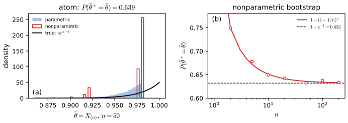
Figure 9.S6 (supplementary). Exercise 9.10. (a) For one \(\Unif(0,1)\) sample of size 50, 20 000 parametric and nonparametric bootstrap replications of \(X_{(n)}\), with the true density \(nt^{n-1}\) of \(\hth\). (b) The probability that a nonparametric bootstrap sample contains the maximum, \(1-(1-1/n)^n\), and its limit \(1-e^{-1}\); circles are simulated frequencies. Not a figure of the book. Code: ch09_parametric_inference.py, fig_9_s6. Download: PDF · SVG
Demonstrations for this chapter
Each demonstration runs in the browser and links back to these notes. The ▶ Demo boxes above open them already set to the case under discussion.
| Demonstration | What you can see | Sections and results |
|---|---|---|
| Fisher information and the Wald interval | For Bernoulli, Poisson, Exponential and Normal-scale samples: the log-likelihood with its quadratic approximation from the Fisher information, the Wald interval on the parameter scale and on the log or logit scale, the likelihood-ratio interval, and the exact coverage of both Wald intervals against the parameter and against \(n\). Presets: 1 Example 9.20; 2 a rare event; 3 Example 9.22; 4 an Exponential rate (a pivot); 5 Example 9.26. | 9.7, 9.9; Theorem 9.19, Filling the gap 9.10 |
| Asymptotic normality and efficiency of the MLE | Simulated sampling distributions of the MLE and of a competitor with their Normal limits, and \(n\times\)MSE against \(n\) with the Cramér–Rao level \(1/I\). Presets: 1 mean against median; 2 Cauchy location; 3 Gamma shape, MLE against moments; 4 Exercise 9.6; 5 the Uniform endpoint. | 9.2, 9.7, 9.8; Theorem 9.18, Filling the gaps 9.11–9.13 |
| Computing the MLE: Newton–Raphson against EM | Censored Normal data (Newton's parabola and EM's lower parabola on the log-likelihood) and the two-Normal mixture of Example 9.50 (both paths on a contour map, including Old Faithful); distance to the MLE against the iteration, with the EM rate predicted by the missing information. Presets: 1 heavy censoring; 2 light censoring; 3 Example 9.50; 4 a saddle point; 5 Old Faithful. | 9.13.4; Filling the gaps 9.23, 9.24 |
Related demonstrations in the companion courses: the first-year maximum likelihood demo, the likelihood for count data demo of Statistical Methods for Modern Biology, the EM lower-bound demo of Bayesian and Probabilistic Machine Learning and the EM and ELBO steps demo of Foundations of Deep Learning; in this course, the delta method demo of Chapter 5. The Python code that produces every figure of this page is code/ch09_parametric_inference.py (see the code index).
References
- Wasserman, L. (2004). All of Statistics: A Concise Course in Statistical Inference. Springer, New York. Chapter 9, pp. 119–148. www.stat.cmu.edu/~larry/all-of-statistics (data and errata).
- Azzalini, A. and Bowman, A. W. (1990). A look at some data on the Old Faithful geyser. Applied Statistics, 39(3), 357–365.
- Casella, G. and Berger, R. L. (2002). Statistical Inference, 2nd edition. Duxbury, Pacific Grove.
- Cramér, H. (1946). Mathematical Methods of Statistics. Princeton University Press, Princeton.
- Dempster, A. P., Laird, N. M. and Rubin, D. B. (1977). Maximum likelihood from incomplete data via the EM algorithm. Journal of the Royal Statistical Society, Series B, 39(1), 1–38.
- Efron, B. and Hinkley, D. V. (1978). Assessing the accuracy of the maximum likelihood estimator: observed versus expected Fisher information. Biometrika, 65(3), 457–483.
- Hájek, J. (1972). Local asymptotic minimax and admissibility in estimation. Proceedings of the Sixth Berkeley Symposium on Mathematical Statistics and Probability, 1, 175–194.
- Halmos, P. R. and Savage, L. J. (1949). Application of the Radon–Nikodym theorem to the theory of sufficient statistics. The Annals of Mathematical Statistics, 20(2), 225–241.
- Huber, P. J. (1967). The behavior of maximum likelihood estimates under nonstandard conditions. Proceedings of the Fifth Berkeley Symposium on Mathematical Statistics and Probability, 1, 221–233.
- Le Cam, L. (1953). On some asymptotic properties of maximum likelihood estimates and related Bayes' estimates. University of California Publications in Statistics, 1, 277–330.
- Lehmann, E. L. and Casella, G. (1998). Theory of Point Estimation, 2nd edition. Springer, New York.
- McLachlan, G. J. and Krishnan, T. (2008). The EM Algorithm and Extensions, 2nd edition. Wiley, Hoboken.
- Neyman, J. and Scott, E. L. (1948). Consistent estimates based on partially consistent observations. Econometrica, 16(1), 1–32.
- Orchard, T. and Woodbury, M. A. (1972). A missing information principle: theory and applications. Proceedings of the Sixth Berkeley Symposium on Mathematical Statistics and Probability, 1, 697–715.
- van der Vaart, A. W. (1998). Asymptotic Statistics. Cambridge University Press, Cambridge.
- Wald, A. (1949). Note on the consistency of the maximum likelihood estimate. The Annals of Mathematical Statistics, 20(4), 595–601.
- White, H. (1982). Maximum likelihood estimation of misspecified models. Econometrica, 50(1), 1–25.
- Wu, C. F. J. (1983). On the convergence properties of the EM algorithm. The Annals of Statistics, 11(1), 95–103.
- Zehna, P. W. (1966). Invariance of maximum likelihood estimators. The Annals of Mathematical Statistics, 37(3), 744.
The numerical statements in the text (the asymptotic covariance of the Gamma moment estimator and the values given by the printed formula, the Kullback–Leibler closed forms, the information identities for the four demo models, the exact coverage of the Wald intervals, the variances of the median and of the Cauchy MLE, Hodges' risk, the Cramér–Rao and Rao–Blackwell variances, the standard error of Example 9.29, the bootstrap facts, the EM rates and the Old Faithful fit, and the solutions of the exercises) were confirmed numerically.