Inequalities
Most probabilities that matter in statistics cannot be computed exactly: the distribution of an average depends on the unknown distribution of the data. An inequality replaces the exact value by a bound that needs only a little information, such as a mean, a variance or the range of the observations. This short chapter collects the inequalities used throughout the rest of the course: Markov's and Chebyshev's, which need one or two moments; Hoeffding's, which needs only bounded observations and gives exponentially small tails, and with it a confidence interval for a proportion valid for every sample size; Mill's bound on the normal tail; and two inequalities for expectations, Cauchy-Schwarz and Jensen. They drive the law of large numbers (Chapter 5), confidence intervals (Chapter 6) and the theory of classification (Chapter 22).
Ch. 1 Probability Ch. 2 Random variables Ch. 3 Expectation Ch. 4 Inequalities Ch. 5 Convergence Ch. 6 Models and inference Ch. 7 Estimating the CDF Ch. 8 Bootstrap Ch. 9 Parametric inference Ch. 10 Hypothesis testing Ch. 11 Bayesian inference Ch. 12 Decision theory Ch. 13 Regression Ch. 14 Multivariate models Ch. 15 Independence Ch. 16 Causal inference Ch. 17 Directed graphs Ch. 18 Undirected graphs Ch. 19 Log-linear models Ch. 20 Curve estimation Ch. 21 Orthogonal functions Ch. 22 Classification Ch. 23 Stochastic processes Ch. 24 Simulation
How to read these notes
They follow the book. Sections carry the book's numbers (4.1 to 4.5), theorems and examples keep the book's numbers (Theorem 4.1 to 4.9, Examples 4.3 and 4.6), and every displayed equation that appears in the book carries the book's own equation number, e.g. \((4.3)\). Results added here are numbered from 4.10 on and marked as additions.
Filling the gaps. The book proves Markov's, Chebyshev's and Jensen's inequalities in a few lines (assuming a density or a tangent line), proves Hoeffding's inequality in an appendix with one step left unproved, and states Mill's and the Cauchy-Schwarz inequalities and the basic facts about convex functions without proof. Each gets a complete argument here, in an orange Filling the gap box or a proof; they start hidden: open one with its bar, or use the button below.
Figures and demonstrations. The chapter has no figures of its own. The seven figures here are supplementary (numbered 4.S1 to 4.S7): they compare the bounds with the exact probabilities and answer the computer exercises, and are made by the Python code. The ▶ Demo boxes open an interactive demonstration already set to the case being discussed.
Main reference
L. Wasserman, All of Statistics: A Concise Course in Statistical Inference, Springer (2004), Chapter 4, pages 63–69 (book website: www.stat.cmu.edu/~larry/all-of-statistics). Section, theorem, equation and exercise numbers below refer to this book. Further reading is listed in the references.
The explanations, derivations, figures and code are my own; equations are cited by their numbers in the book.
Companion courses
Parts of this chapter appear elsewhere on this site:
- Markov's and Chebyshev's inequalities and the weak law of large numbers, at an introductory level: first-year notes, Theorem 0.4 and Section 0.3; the normal-approximation (Wald) interval for a proportion that Hoeffding's interval is compared with: Section 3.5.
- Jensen's inequality and the Kullback-Leibler divergence: Bayesian and Probabilistic Machine Learning, mathematical toolkit, Section 1.1 and Section 1.2 (several variables, and the evidence lower bound); Foundations of Deep Learning, Filling the gap 2.16 (convexity and Jensen's equality case) and Result 2.10 (Gibbs' inequality, and why minimising KL is maximum likelihood), with the multivariate supporting-plane argument in Appendix B, Result B.3.
- Where concentration inequalities lead: Statistical Learning: Theory and Methods, Section 7.9 and Filling the gap 7.7 (Vapnik-Chervonenkis bounds, which combine a Hoeffding-type tail bound with a union bound over a class of classifiers).
Where a proof there is the same, these notes give it briefly and link to it. New here: the general (density-free) proofs with the cases of equality, the one-sided Chebyshev inequality, the optimal Chernoff exponent for a proportion and a matching lower bound, the coverage and price of Hoeffding's interval, a lower bound to go with Mill's inequality, and the maximal inequality for Gaussians.
The chapter at a glance
- Markov (Theorem 4.1): for \(X\ge0\), \(\P(X\ge t)\le\E(X)/t\); attained by variables on \(\{0,t\}\) (gap 4.1). Applied to \(\phi(X)\) it gives every other bound of the chapter (gap 4.2).
- Chebyshev (Theorem 4.2): \(\P(|X-\mu|\ge t)\le\sigma^2/t^2\); sharp, with a sharper one-sided form (gap 4.3).
- Hoeffding (Theorems 4.4 and 4.5): averages of bounded variables have tails at most \(2e^{-2n\epsilon^2}\); proof in Section 4.4 via Hoeffding's lemma (Result 4.12). The Chernoff bound \(e^{-n\kl(p+\epsilon,p)}\) is sharper and has the exact exponent (gap 4.5).
- An interval for a proportion (Definition 4.1): \(\hat p\pm\sqrt{\log(2/\alpha)/(2n)}\) has coverage at least \(1-\alpha\) for every \(n\) and \(p\), at the price of being about 40% longer than the normal interval (gap 4.6).
- Mill (Theorem 4.7): \(\P(|Z|>t)\le\sqrt{2/\pi}\,e^{-t^2/2}/t\), and the ratio to the truth tends to 1.
- Cauchy-Schwarz (Theorem 4.8) and Jensen (Theorem 4.9), with the facts about convex functions they rest on (gap 4.8) and their consequences: means, moments (gap 4.9), the Kullback-Leibler divergence (Result 4.10) and the maximum of Gaussians (Result 4.11).
Notation. \(\E\), \(\P\) and \(\V\) are expectation, probability and variance. \(\Xbar=n^{-1}\sum_{i=1}^nX_i\). \(Z\sim N(0,1)\) has density \(\phi(z)=e^{-z^2/2}/\sqrt{2\pi}\) and distribution function \(\Phi\). \(\ind_A\) is the indicator of an event \(A\). \(\kl(q,p)=q\log\frac qp+(1-q)\log\frac{1-q}{1-p}\) is the Kullback-Leibler divergence between Bernoulli(\(q\)) and Bernoulli(\(p\)). Logarithms are natural.
Prerequisites. Expectation, variance, independence and moment generating functions (Chapters 2 and 3 of the book).
4.1 Probability Inequalities
p. 63 An inequality is useful when the quantity it bounds is hard to compute and the quantity it uses is easy. All the probability inequalities of this section come from a single idea, Markov's inequality, applied to a well-chosen function of the random variable.
See also (first-year notes): Markov and Chebyshev, Theorem 0.4.
Theorem 4.1 (Markov's inequality) p. 63, (4.1)
Let \(X\) be a non-negative random variable with \(\E(X)\lt\infty\). For every \(t\gt0\),
\[ \P(X>t)\le\frac{\E(X)}{t}. \tag{4.1} \]In fact the stronger statement \(\P(X\ge t)\le\E(X)/t\) holds.
Proof (for any non-negative random variable, with or without a density)
Compare two random variables pointwise. On the event \(\{X\ge t\}\) we have \(X\ge t=t\,\ind_{\{X\ge t\}}\); off it, \(X\ge0=t\,\ind_{\{X\ge t\}}\) because \(X\) is non-negative. So
\[ t\,\ind_{\{X\ge t\}}\le X\quad\text{everywhere}. \]Expectation is monotone, and \(\E(\ind_A)=\P(A)\), so \(t\,\P(X\ge t)\le\E(X)\). Divide by \(t\gt0\). Since \(\{X>t\}\subseteq\{X\ge t\}\), (4.1) follows. ∎
The book's proof splits \(\int_0^\infty xf(x)\,\d x\) at \(t\) and so assumes a density; the argument above covers discrete and mixed distributions too. It also shows exactly what is thrown away: \(\E(X)-t\P(X\ge t)=\E\{X\ind_{\{X\lt t\}}\}+\E\{(X-t)\ind_{\{X\ge t\}}\}\), the mass below \(t\) and the overshoot above it.
Filling the gap 4.1: Markov's inequality cannot be improved p. 63
Given only that \(X\ge0\) and \(\E(X)=m\), the bound \(m/t\) is the best possible for \(\P(X\ge t)\) whenever \(t\ge m\), and equality holds exactly for variables taking only the values 0 and \(t\).
Derivation
Attained. Let \(t\ge m\gt0\) and let \(X=t\) with probability \(m/t\) and \(X=0\) otherwise. Then \(\E(X)=t\cdot m/t=m\) and \(\P(X\ge t)=m/t=\E(X)/t\).
Only then. By the identity at the end of the proof, \(\E(X)-t\P(X\ge t)\) is the sum of the expectations of the two non-negative variables \(X\ind_{\{X\lt t\}}\) and \((X-t)\ind_{\{X\ge t\}}\). It is zero if and only if both vanish almost surely, i.e. \(X=0\) whenever \(X\lt t\) and \(X=t\) whenever \(X\ge t\): \(X\in\{0,t\}\) almost surely.
The strict form (4.1). For \(\P(X>t)\) the supremum \(m/t\) over all such \(X\) is approached (put the mass at \(t+\delta\) with probability \(m/(t+\delta)\) and let \(\delta\downarrow0\)) but attained only by \(X\equiv0\), where both sides are 0.
For \(t\lt m\) the bound exceeds 1 and says nothing. Markov's inequality is therefore weak for any particular distribution but unbeatable as a statement about all distributions with a given mean. ∎
Filling the gap 4.2: Markov applied to a function of \(X\) pp. 63–64, 67
Let \(\varphi\ge0\) be non-decreasing with \(\varphi(t)\gt0\). Then for any random variable \(X\) (not necessarily non-negative)
\[ \P(X\ge t)\le\P\{\varphi(X)\ge\varphi(t)\}\le\frac{\E\,\varphi(X)}{\varphi(t)}. \]Three choices give the rest of the chapter: \(\varphi(x)=x^2\) applied to \(|X-\mu|\) is Chebyshev's inequality; \(\varphi(x)=x^k\) applied to \(|X|\) gives the moment bounds \(\P(|X|\ge t)\le\E|X|^k/t^k\) of Exercise 6; and \(\varphi(x)=e^{sx}\) with \(s\gt0\) gives the Chernoff bound
\[ \P(X\ge t)\le\inf_{s\gt0}e^{-st}\,\E\,e^{sX}, \]which is how Hoeffding's inequality is proved (Section 4.4).
Derivation
If \(X\ge t\) then \(\varphi(X)\ge\varphi(t)\) because \(\varphi\) is non-decreasing, so \(\{X\ge t\}\subseteq\{\varphi(X)\ge\varphi(t)\}\). The variable \(\varphi(X)\) is non-negative, so Markov's inequality (Theorem 4.1, in its \(\ge\) form) applies to it at the level \(\varphi(t)\gt0\). The Chernoff bound holds for each \(s\gt0\) separately, so also for the infimum. When \(\E\varphi(X)=\infty\) the bound is true and empty. ∎
Theorem 4.2 (Chebyshev's inequality) p. 64, (4.2)
Let \(\mu=\E(X)\) and \(\sigma^2=\V(X)\lt\infty\). Then for every \(t\gt0\), and, when \(\sigma\gt0\), with \(Z=(X-\mu)/\sigma\) and every \(k\gt0\),
\[ \P(|X-\mu|\ge t)\le\frac{\sigma^2}{t^2}\qquad\text{and}\qquad\P(|Z|\ge k)\le\frac1{k^2}. \tag{4.2} \]In particular \(\P(|Z|\gt2)\le1/4\) and \(\P(|Z|\gt3)\le1/9\).
Proof
The events \(\{|X-\mu|\ge t\}\) and \(\{(X-\mu)^2\ge t^2\}\) are equal. Apply Markov's inequality to the non-negative variable \((X-\mu)^2\), whose mean is \(\sigma^2\): \(\P\{(X-\mu)^2\ge t^2\}\le\sigma^2/t^2\). For the second form put \(t=k\sigma\). ∎
For a normal variable the true values are \(\P(|Z|\gt2)=0.046\) and \(\P(|Z|\gt3)=0.0027\), far below 1/4 and 1/9: Chebyshev's inequality pays for holding for every distribution with the given variance.
Filling the gap 4.3: Chebyshev is sharp, and its one-sided form p. 64
(a) For every \(k\ge1\) there is a distribution with mean \(\mu\) and variance \(\sigma^2\) for which \(\P(|X-\mu|\ge k\sigma)=1/k^2\). (b) Cantelli's inequality: for \(t\gt0\),
\[ \P(X-\mu\ge t)\le\frac{\sigma^2}{\sigma^2+t^2}, \]which is smaller than \(\sigma^2/t^2\) and is also attained by a two-point distribution.
Derivation
(a) Let \(X\) take the values \(\mu-k\sigma\), \(\mu\), \(\mu+k\sigma\) with probabilities \(1/(2k^2)\), \(1-1/k^2\), \(1/(2k^2)\) (a probability distribution because \(k\ge1\)). It is symmetric about \(\mu\), so \(\E(X)=\mu\); its variance is \(2\cdot\frac1{2k^2}(k\sigma)^2=\sigma^2\); and \(\P(|X-\mu|\ge k\sigma)=1/k^2\).
(b) Put \(Y=X-\mu\), so \(\E Y=0\), \(\E Y^2=\sigma^2\). For any \(u\ge0\), \(Y\ge t\) implies \(Y+u\ge t+u\gt0\), hence \((Y+u)^2\ge(t+u)^2\). By Markov's inequality applied to \((Y+u)^2\),
\[ \P(Y\ge t)\le\frac{\E(Y+u)^2}{(t+u)^2}=\frac{\sigma^2+u^2}{(t+u)^2}. \]The right side is minimised at \(u=\sigma^2/t\) (its derivative in \(u\) is \(2(ut-\sigma^2)/(t+u)^3\)), where it equals \(\frac{\sigma^2(t^2+\sigma^2)/t^2}{(t^2+\sigma^2)^2/t^2}=\frac{\sigma^2}{\sigma^2+t^2}\).
Attained. Let \(Y=t\) with probability \(\pi=\sigma^2/(\sigma^2+t^2)\) and \(Y=-\sigma^2/t\) otherwise. Then \(\E Y=t\pi-\frac{\sigma^2}{t}\cdot\frac{t^2}{\sigma^2+t^2}=0\), \(\E Y^2=\frac{t^2\sigma^2+\sigma^4}{\sigma^2+t^2}=\sigma^2\), and \(\P(Y\ge t)=\pi\). ∎
Example 4.3 (the error rate of a classifier) p. 64
A prediction method is tried on \(n\) new cases; \(X_i=1\) if it errs on case \(i\) and 0 otherwise, and the \(X_i\) are independent Bernoulli(\(p\)) with \(p\) the unknown error rate. The observed error rate \(\Xbar\) has variance \(\V(\Xbar)=p(1-p)/n\), because the variance of a sum of independent variables is the sum of the variances. Chebyshev's inequality gives
\[ \P(|\Xbar-p|\gt\epsilon)\le\frac{\V(\Xbar)}{\epsilon^2}=\frac{p(1-p)}{n\epsilon^2}\le\frac1{4n\epsilon^2}, \]since \(p(1-p)=\tfrac14-(p-\tfrac12)^2\le\tfrac14\). For \(\epsilon=0.2\) and \(n=100\) the bound is \(0.0625\). The true probability, for the worst case \(p=1/2\), is \(3.2\times10^{-5}\).
Theorem 4.4 (Hoeffding's inequality) p. 64, (4.3)
Let \(Y_1,\dots,Y_n\) be independent with \(\E(Y_i)=0\) and \(a_i\le Y_i\le b_i\). Let \(\epsilon\gt0\). Then for every \(t\gt0\),
\[ \P\Big(\sum_{i=1}^nY_i\ge\epsilon\Big)\le e^{-t\epsilon}\prod_{i=1}^ne^{t^2(b_i-a_i)^2/8}. \tag{4.3} \]Proof: Section 4.4.
Filling the gap 4.4: the best \(t\), and the form in which Hoeffding's inequality is used pp. 64, 67
With \(D=\sum_i(b_i-a_i)^2\), the best choice in (4.3) is \(t=4\epsilon/D\), and it gives
\[ \P\Big(\sum_{i=1}^nY_i\ge\epsilon\Big)\le\exp\Big(-\frac{2\epsilon^2}{D}\Big). \]Consequently, if \(X_1,\dots,X_n\) are independent with \(a\le X_i\le b\) and \(\mu=\E(\Xbar)\) (the \(X_i\) need not have the same distribution),
\[ \P(\Xbar-\mu\ge\epsilon)\le e^{-2n\epsilon^2/(b-a)^2},\qquad \P(|\Xbar-\mu|\ge\epsilon)\le2e^{-2n\epsilon^2/(b-a)^2}. \]Derivation
The logarithm of the right side of (4.3) is \(h(t)=-t\epsilon+t^2D/8\), a convex parabola with \(h'(t)=-\epsilon+tD/4=0\) at \(t^*=4\epsilon/D\gt0\), where \(h(t^*)=-4\epsilon^2/D+2\epsilon^2/D=-2\epsilon^2/D\).
For the averages, put \(Y_i=(X_i-\E X_i)/n\). These are independent, have mean 0, and lie in an interval of length \((b-a)/n\), so \(D=n(b-a)^2/n^2=(b-a)^2/n\), and \(\{\Xbar-\mu\ge\epsilon\}=\{\sum Y_i\ge\epsilon\}\). The lower tail follows by applying the same bound to \(-Y_i\), which also have mean 0 and range \((b-a)/n\); the two-sided bound is the sum of the two (a union bound). ∎
What the bound ignores. The variance does not appear: Hoeffding's bound is exactly what one gets from a variable with the largest variance compatible with the range, \((b-a)^2/4\). When the variance is much smaller, Chebyshev's inequality can win for moderate \(n\) (Figure 4.S1(c)); bounds that use both the range and the variance (Bernstein's) are in the references.
Theorem 4.5 (Hoeffding's inequality for a proportion) p. 65, (4.4)
Let \(X_1,\dots,X_n\) be independent Bernoulli(\(p\)). Then for every \(\epsilon\gt0\),
\[ \P(|\Xbar-p|\gt\epsilon)\le2e^{-2n\epsilon^2}. \tag{4.4} \]Proof: Section 4.4; it is also the case \(a=0\), \(b=1\) of Filling the gap 4.4.
Example 4.6 p. 65
For \(n=100\) and \(\epsilon=0.2\), Hoeffding's inequality gives \(\P(|\Xbar-p|\gt0.2)\le2e^{-8}=0.00067\), against 0.0625 from Chebyshev. The sharper Chernoff bound of Filling the gap 4.5 gives 0.00053, and the exact probability at \(p=1/2\) is \(3.2\times10^{-5}\): even the exponential bounds are off by a factor of about 20, but they are off by a constant factor, while Chebyshev's \(1/n\) rate is off by an exponential one.
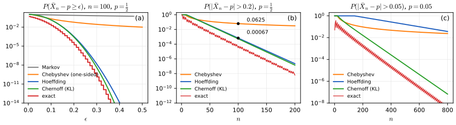
fig_4_s1. Supplementary figure; illustrates Wasserman (2004), Examples 4.3 and 4.6 and Exercise 4.3. Download: PDF · SVGFilling the gap 4.5: the Chernoff bound for a proportion, and the exact exponent pp. 64–65, 67
Let \(S=n\Xbar\sim\Bin(n,p)\) with \(0\lt p\lt1\), and \(p\lt q\lt1\). Then
\[ \text{(i)}\ \ \P(\Xbar\ge q)\le e^{-n\kl(q,p)},\qquad \text{(ii)}\ \ \kl(q,p)\ge2(q-p)^2,\qquad \text{(iii)}\ \ \P(\Xbar\ge q)\ge\frac{e^{-n\kl(q,p)}}{n+1}\ \text{ if } nq \text{ is an integer}. \]So (i) implies Hoeffding's bound \(e^{-2n\epsilon^2}\) for \(q=p+\epsilon\) and is never worse; and by (iii) its exponent cannot be improved: \(\frac1n\log\P(\Xbar\ge q)\to-\kl(q,p)\). For small \(\epsilon\), \(\kl(p+\epsilon,p)\approx\epsilon^2/\{2p(1-p)\}\), which equals Hoeffding's \(2\epsilon^2\) only at \(p=1/2\): Hoeffding's exponent is right for a fair coin and too small otherwise.
Derivation
(i) Optimising the Chernoff bound. By Filling the gap 4.2 with \(\varphi(x)=e^{sx}\), and \(\E e^{sS}=(1-p+pe^s)^n\) (independence),
\[ \P(S\ge nq)\le e^{-snq}(1-p+pe^s)^n=e^{nf(s)},\qquad f(s)=-sq+\log(1-p+pe^s). \]\(f\) is convex (\(f''(s)=\rho(1-\rho)\ge0\) with \(\rho=pe^s/(1-p+pe^s)\)), and \(f'(s)=-q+\rho=0\) when \(e^s=\frac{q(1-p)}{p(1-q)}\), which is greater than 1 because \(q\gt p\), so \(s\gt0\) is allowed. There \(1-p+pe^s=1-p+\frac{q(1-p)}{1-q}=\frac{1-p}{1-q}\) and
\[ f(s)=-q\log\frac{q(1-p)}{p(1-q)}+\log\frac{1-p}{1-q}=-q\log\frac qp-(1-q)\log\frac{1-q}{1-p}=-\kl(q,p). \](ii) A Pinsker-type inequality. Fix \(p\) and let \(h(q)=\kl(q,p)-2(q-p)^2\) on \((0,1)\). Then \(h(p)=0\); \(h'(q)=\log\frac qp-\log\frac{1-q}{1-p}-4(q-p)\), so \(h'(p)=0\); and \(h''(q)=\frac1q+\frac1{1-q}-4=\frac1{q(1-q)}-4\ge0\) since \(q(1-q)\le\frac14\). A convex function with a stationary point at \(p\) has its minimum there, so \(h\ge0\). (By continuity it also holds at \(q=0,1\).)
(iii) A matching lower bound. Let \(k=nq\), an integer with \(np\lt k\lt n\) (for \(k=n\) both sides are explicit: \(\P(S=n)=p^n=e^{-n\kl(1,p)}\)). Write \(b_r(j)=\binom nj r^j(1-r)^{n-j}\). The ratio \(b_q(j+1)/b_q(j)=\frac{(n-j)q}{(j+1)(1-q)}\) is at least 1 exactly when \(j\le(n+1)q-1=k-1+q\), i.e. when \(j\le k-1\); so \(b_q\) increases up to \(j=k\) and decreases after it, and \(b_q(k)\) is the largest of \(n+1\) probabilities that add up to 1: \(b_q(k)\ge1/(n+1)\). Now
\[ \P(S\ge k)\ge b_p(k)=b_q(k)\Big(\frac pq\Big)^k\Big(\frac{1-p}{1-q}\Big)^{n-k}=b_q(k)\,e^{-n\kl(q,p)}\ge\frac{e^{-n\kl(q,p)}}{n+1}. \]Taking logarithms, \(-\kl(q,p)-\frac{\log(n+1)}n\le\frac1n\log\P(\Xbar\ge q)\le-\kl(q,p)\), and the squeeze gives the limit along such \(n\); continuity of \(\kl\) in \(q\) extends it to all \(n\). The small-\(\epsilon\) form comes from \(\kl(p+\epsilon,p)=\frac{\epsilon^2}{2p(1-p)}+O(\epsilon^3)\), a second-order Taylor expansion of \(q\mapsto\kl(q,p)\) at \(q=p\) using \(h''\) above. ∎
This is the method of types of information theory (Cover and Thomas, 2006, Chapter 11). The Kullback-Leibler divergence reappears in Section 4.2, Result 4.10.
p. 65 Hoeffding's inequality turns directly into an interval estimate for \(p\), developed fully in Chapter 6. Fix \(\alpha\in(0,1)\) and put
\[ \epsilon_n=\sqrt{\frac1{2n}\log\Big(\frac2\alpha\Big)},\qquad\text{so that}\qquad2e^{-2n\epsilon_n^2}=\alpha. \]By Theorem 4.5, the random interval \(C=(\Xbar-\epsilon_n,\Xbar+\epsilon_n)\) satisfies \(\P(p\notin C)=\P(|\Xbar-p|\ge\epsilon_n)\le\alpha\) (Theorem 4.5 with \(\epsilon\) slightly below \(\epsilon_n\), then a limit, handles the "\(\ge\)"), so \(\P(p\in C)\ge1-\alpha\).
Definition 4.1 (confidence interval, first version) p. 65
A random interval \(C=C(X_1,\dots,X_n)\) is a \(1-\alpha\) confidence interval for a parameter \(p\) if \(\P_p(p\in C)\ge1-\alpha\) for every value of \(p\). Here \(C\) is random and \(p\) is fixed: the probability statement is about the procedure, not about \(p\).
Filling the gap 4.6: what Hoeffding's interval guarantees, and what it costs p. 65 and Exercise 4
(a) The coverage is at least \(1-\alpha\) for every \(n\ge1\) and every \(p\in[0,1]\). (b) Truncating \(C\) to \([0,1]\) changes nothing in (a). (c) The length is \(2\epsilon_n=\sqrt{2\log(2/\alpha)/n}\), not random; it is at most \(L\) exactly when \(n\ge2\log(2/\alpha)/L^2\). (d) Compared with the normal-approximation interval \(\Xbar\pm z_{\alpha/2}\sqrt{\Xbar(1-\Xbar)/n}\), it is longer by the factor \(\sqrt{\log(2/\alpha)/2}\,/\,\{z_{\alpha/2}\sqrt{p(1-p)}\}\) for large \(n\), at least 1.386 when \(\alpha=0.05\). (e) For large \(n\) its coverage tends to \(2\Phi\big(\sqrt{\log(2/\alpha)/2}/\sigma\big)-1\) with \(\sigma^2=p(1-p)\), which is at least \(2\Phi\big(\sqrt{2\log(2/\alpha)}\big)-1=0.9934\) when \(\alpha=0.05\): the interval is conservative.
Derivation
(a) Theorem 4.5 holds for every \(n\) and \(p\) (for \(p\in\{0,1\}\), \(\Xbar=p\) and coverage is 1). Unlike the normal interval, nothing is approximate.
(b) \(p\in[0,1]\), so \(p\in C\) if and only if \(p\in C\cap[0,1]\).
(c) Solve \(2\epsilon_n\le L\), i.e. \(\frac{2\log(2/\alpha)}{n}\le L^2\). For \(\alpha=L=0.05\) this is \(n\ge2\log(40)/0.0025=2951.1\), so \(n=2952\) (Exercise 4(c)).
(d) By the law of large numbers (Chapter 5) \(\Xbar(1-\Xbar)\to p(1-p)\), so the normal half-width behaves like \(z_{\alpha/2}\sqrt{p(1-p)/n}\); divide \(\epsilon_n\) by it. The factor is smallest at \(p=1/2\), where it is \(\sqrt{\log 40/2}/(1.96\times0.5)=1.386\).
(e) \(\P(|\Xbar-p|\lt\epsilon_n)=\P\big(|\sqrt n(\Xbar-p)/\sigma|\lt\sqrt{\log(2/\alpha)/2}/\sigma\big)\) and the central limit theorem (Chapter 5) gives the limit, a continuous distribution function evaluated at a fixed point. It is increasing in \(1/\sigma\) and \(\sigma\le1/2\). For \(p=0.4\) the limit is 0.9944, and the exact coverage at \(n=10{,}000\) is 0.9943 (Figure 4.S2). ∎
The normal interval's coverage, by contrast, is only approximately \(1-\alpha\), and can be far lower: for \(n=50\) and \(p=0.02\) no success is observed with probability \(0.98^{50}=0.36\), the interval is then the single point 0, and its coverage is 0.64. Better intervals (Wilson's, or the exact Clopper-Pearson interval) are discussed by Brown, Cai and DasGupta (2001).
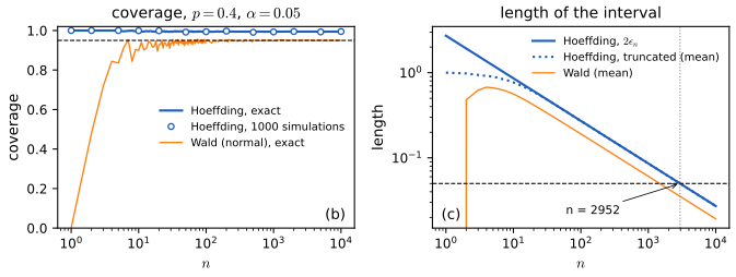
fig_4_s2. Supplementary figure; answers Wasserman (2004), Exercise 4.4. Download: PDF · SVGp. 65 The next inequality bounds normal tails, which have no closed form.
Theorem 4.7 (Mill's inequality) p. 65; Exercise 5
Let \(Z\sim N(0,1)\). For every \(t\gt0\),
\[ \sqrt{\frac2\pi}\,\frac{t}{1+t^2}\,e^{-t^2/2}\ \le\ \P(|Z|\gt t)\ \le\ \sqrt{\frac2\pi}\,\frac{e^{-t^2/2}}{t}. \]The right inequality is the book's; the left one (added here) shows that the ratio of the bound to the true tail tends to 1 as \(t\to\infty\).
Proof
By symmetry \(\P(|Z|\gt t)=2\P(Z\gt t)=2\int_t^\infty\phi(x)\,\d x\), and \(\phi'(x)=-x\phi(x)\).
Upper bound. On \(x\ge t\gt0\), \(x/t\ge1\), so
\[ \int_t^\infty\phi(x)\,\d x\le\int_t^\infty\frac xt\,\phi(x)\,\d x=\frac1t\Big[-\phi(x)\Big]_t^\infty=\frac{\phi(t)}t. \]Doubling, \(\P(|Z|\gt t)\le2\phi(t)/t=\sqrt{2/\pi}\,e^{-t^2/2}/t\).
Lower bound. Differentiate: \(\frac{\d}{\d x}\big\{-\phi(x)/x\big\}=\frac{x^2\phi(x)+\phi(x)}{x^2}=\big(1+x^{-2}\big)\phi(x)\). Integrating from \(t\) to \(\infty\),
\[ \frac{\phi(t)}t=\int_t^\infty\big(1+x^{-2}\big)\phi(x)\,\d x\le\big(1+t^{-2}\big)\int_t^\infty\phi(x)\,\d x, \]so \(\P(Z\gt t)\ge\frac{t}{1+t^2}\phi(t)\); double it. The two bounds differ by the factor \(1+t^{-2}\to1\). ∎
Mill's bound is the classical "Mills ratio" estimate (after Mills, 1926). It is much sharper than the Chernoff bound \(\P(|Z|\gt t)\le2e^{-t^2/2}\) (from \(\E e^{sZ}=e^{s^2/2}\)) as soon as \(t\gt1/\sqrt{2\pi}\approx0.40\), and than any moment bound (Figure 4.S3).
Filling the gap 4.7: moment bounds for the normal tail (Exercise 6), and why they beat Chernoff p. 68
(a) \(\E|Z|^k=2^{k/2}\Gamma\big(\frac{k+1}2\big)/\sqrt\pi\) for \(k\gt-1\): 0.798, 1, 1.596, 3, 6.383 for \(k=1,\dots,5\). (b) For any \(X\ge0\) and \(t\gt0\), the best moment bound is at least as good as the best Chernoff bound:
\[ \inf_{k=0,1,2,\dots}\frac{\E X^k}{t^k}\le\inf_{s\gt0}e^{-st}\,\E e^{sX}. \]Derivation
(a) \(\E|Z|^k=2\int_0^\infty x^k\phi(x)\,\d x\). Substitute \(u=x^2/2\), \(x=\sqrt{2u}\), \(\d x=\d u/\sqrt{2u}\): \(\E|Z|^k=\frac{2}{\sqrt{2\pi}}\int_0^\infty(2u)^{k/2}e^{-u}\frac{\d u}{\sqrt{2u}}=\frac{2^{k/2}}{\sqrt\pi}\int_0^\infty u^{(k-1)/2}e^{-u}\,\d u\), and the last integral is \(\Gamma\big(\frac{k+1}2\big)\).
(b) Let \(m\) be the infimum on the left, so \(\E X^k\ge m\,t^k\) for every \(k\). By the exponential series and monotone convergence (all terms are non-negative), \(\E e^{sX}=\sum_k\frac{s^k\E X^k}{k!}\ge m\sum_k\frac{(st)^k}{k!}=m\,e^{st}\). Rearranged, \(m\le e^{-st}\E e^{sX}\) for every \(s\gt0\). ∎
For \(X=|Z|\), \(\E e^{s|Z|}=2e^{s^2/2}\Phi(s)\le2e^{s^2/2}\), so the best moment bound is below \(2e^{-t^2/2}\). At \(t=3\): the best real order is \(k\approx9\), with bound 0.0156; Mill gives 0.00295 and the truth is 0.00270. Each moment bound decays only polynomially in \(t\), so for any fixed \(k\) it is eventually much worse than Mill's.
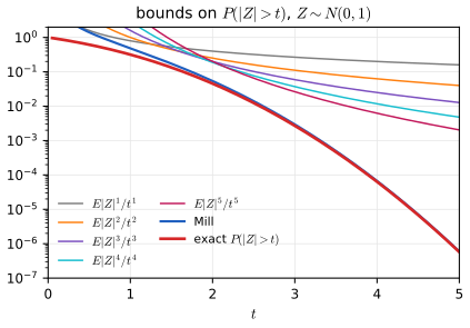
fig_4_s3. Supplementary figure; answers Wasserman (2004), Exercise 4.6. Download: PDF · SVG4.2 Inequalities For Expectations
p. 66 The second group of inequalities compares expectations rather than bounding probabilities.
Theorem 4.8 (Cauchy-Schwarz inequality) p. 66, (4.5)
If \(X\) and \(Y\) have finite variances (equivalently, \(\E X^2\lt\infty\) and \(\E Y^2\lt\infty\)), then \(\E|XY|\) is finite and
\[ \E|XY|\le\sqrt{\E(X^2)\,\E(Y^2)}. \tag{4.5} \]Equality holds if and only if \(|Y|=c|X|\) almost surely for a constant \(c\ge0\), or \(X=0\) almost surely. Consequently \(|\E(XY)|\le\sqrt{\E X^2\,\E Y^2}\) and \(|\Cov(X,Y)|\le\sqrt{\V(X)\V(Y)}\), so a correlation lies in \([-1,1]\).
Proof
Finiteness. \(0\le(|X|-|Y|)^2\) gives \(|XY|\le\tfrac12(X^2+Y^2)\), which has finite expectation.
The inequality. If \(\E X^2=0\), then \(X=0\) almost surely (a non-negative variable with mean zero vanishes almost surely), so both sides are 0. Otherwise, for every real \(\lambda\),
\[ 0\le\E\big(\lambda|X|-|Y|\big)^2=\lambda^2\E X^2-2\lambda\E|XY|+\E Y^2 . \]A quadratic in \(\lambda\) with positive leading coefficient that is never negative has at most one real root, so its discriminant is not positive: \(4(\E|XY|)^2-4\E X^2\,\E Y^2\le0\), which is (4.5).
Equality. If the discriminant is zero, the quadratic vanishes at \(\lambda=c=\E|XY|/\E X^2\), so \(\E(c|X|-|Y|)^2=0\) and \(|Y|=c|X|\) almost surely; conversely \(|Y|=c|X|\) makes both sides of (4.5) equal to \(c\,\E X^2\).
Consequences. \(|\E(XY)|\le\E|XY|\). Apply (4.5) to \(X-\E X\) and \(Y-\E Y\) for the covariance; equality there means \(|Y-\E Y|=c|X-\E X|\), and with the sign condition of \(|\E(XY)|=\E|XY|\), that \(Y\) is an affine function of \(X\). ∎
p. 66 The book defines convexity in words and then uses two facts about convex functions "that can be shown". Here is the definition, and the facts with proofs.
Definition 4.2 (convex and concave functions) p. 66
A function \(g\) on an interval \(I\) is convex if for all \(x,y\in I\) and \(\alpha\in[0,1]\),
\[ g\big(\alpha x+(1-\alpha)y\big)\le\alpha g(x)+(1-\alpha)g(y), \]i.e. every chord lies on or above the graph; strictly convex if the inequality is strict whenever \(x\ne y\) and \(0\lt\alpha\lt1\). \(g\) is concave if \(-g\) is convex. Examples: \(x^2\), \(e^x\), \(|x|\) and, on \((0,\infty)\), \(1/x\), \(-\log x\), \(x\log x\) are convex; \(-x^2\) and \(\log x\) are concave.
Filling the gap 4.8: second derivatives, chords and supporting lines p. 66
(a) If \(g\) is differentiable on an interval and \(g'\) is non-decreasing (in particular, if \(g''\ge0\)), then \(g\) is convex. (b) Three-chord lemma: if \(g\) is convex and \(x\lt z\lt y\) in \(I\), then
\[ \frac{g(z)-g(x)}{z-x}\le\frac{g(y)-g(x)}{y-x}\le\frac{g(y)-g(z)}{y-z}. \](c) Supporting lines: if \(g\) is convex on an open interval \(I\) and \(x_0\in I\), there is a slope \(b\) with \(g(x)\ge g(x_0)+b(x-x_0)\) for all \(x\in I\). If \(g\) is differentiable at \(x_0\), \(b=g'(x_0)\) (the tangent line); at a corner any slope between the left and right derivatives works. If \(g\) is strictly convex, the inequality is strict for \(x\ne x_0\).
Proofs
(a) Let \(x\lt y\), \(\alpha\in(0,1)\) and \(z=\alpha x+(1-\alpha)y\), so \(z-x=(1-\alpha)(y-x)\) and \(y-z=\alpha(y-x)\). By the mean value theorem there are \(\xi_1\in(x,z)\), \(\xi_2\in(z,y)\) with \(g(z)-g(x)=g'(\xi_1)(z-x)\) and \(g(y)-g(z)=g'(\xi_2)(y-z)\), and \(g'(\xi_1)\le g'(\xi_2)\). Hence
\[ \alpha\{g(z)-g(x)\}=\alpha(1-\alpha)(y-x)g'(\xi_1)\le\alpha(1-\alpha)(y-x)g'(\xi_2)=(1-\alpha)\{g(y)-g(z)\}, \]which rearranges to \(g(z)\le\alpha g(x)+(1-\alpha)g(y)\). If \(g''\ge0\), \(g'\) is non-decreasing by the mean value theorem applied to \(g'\).
(b) Write \(z=\alpha x+(1-\alpha)y\) with \(\alpha=\frac{y-z}{y-x}\), \(1-\alpha=\frac{z-x}{y-x}\). Convexity, minus \(g(x)\): \(g(z)-g(x)\le(1-\alpha)\{g(y)-g(x)\}=\frac{z-x}{y-x}\{g(y)-g(x)\}\), the first inequality. Convexity, minus \(g(y)\): \(g(z)-g(y)\le\alpha\{g(x)-g(y)\}\), i.e. \(g(y)-g(z)\ge\frac{y-z}{y-x}\{g(y)-g(x)\}\), the second.
(c) By (b), the slope \(s(u,v)=\frac{g(v)-g(u)}{v-u}\) increases in each argument, and for \(u\lt x_0\lt v\), \(s(u,x_0)\le s(x_0,v)\). So \(b_-=\sup_{u\lt x_0}s(u,x_0)\) (the left derivative) and \(b_+=\inf_{v\gt x_0}s(x_0,v)\) (the right derivative) are finite, because \(I\) is open and there are points on both sides, and \(b_-\le b_+\). Take any \(b\in[b_-,b_+]\). For \(v\gt x_0\): \(s(x_0,v)\ge b_+\ge b\), i.e. \(g(v)\ge g(x_0)+b(v-x_0)\). For \(u\lt x_0\): \(s(u,x_0)\le b_-\le b\), i.e. \(g(x_0)-g(u)\le b(x_0-u)\), which is \(g(u)\ge g(x_0)+b(u-x_0)\). If \(g\) is differentiable at \(x_0\), \(b_-=b_+=g'(x_0)\).
Strictness. Let \(L(x)=g(x_0)+b(x-x_0)\) and suppose \(g(x_1)=L(x_1)\) for some \(x_1\ne x_0\). At the midpoint \(z\), strict convexity gives \(g(z)\lt\tfrac12g(x_0)+\tfrac12g(x_1)=\tfrac12L(x_0)+\tfrac12L(x_1)=L(z)\), contradicting \(g\ge L\). ∎
For \(|x|\) at 0, \(b_-=-1\), \(b_+=1\): every line through the origin with slope in \([-1,1]\) supports the graph, and no tangent exists. (A convex function on an open interval is also continuous, by the same slope bounds; the proofs above do not need this.)
See also (companion courses): Foundations of Deep Learning, Filling the gap 2.16 (convexity and second derivatives) and Appendix B, Result B.3 (tangent planes in several variables).
Theorem 4.9 (Jensen's inequality) p. 66, (4.6)–(4.7)
Let \(g\) be convex on an open interval \(I\), and \(X\) a random variable with \(\P(X\in I)=1\) and \(\E|X|\lt\infty\). Then \(\E X\in I\), \(\E g(X)\) is well defined (possibly \(+\infty\)), and
\[ \E g(X)\ge g(\E X). \tag{4.6} \]If \(g\) is concave, \(\E g(X)\le g(\E X)\) (4.7). If \(g\) is strictly convex and \(\E g(X)\lt\infty\), equality holds only if \(X\) is almost surely constant.
Proof
The mean is in \(I\). Say \(I=(c,d)\) with \(-\infty\le c\lt d\le\infty\). If \(c\) is finite, \(X-c\gt0\) almost surely, so \(\E X-c\ge0\), and \(\E X=c\) would make the positive variable \(X-c\) have mean 0, which is impossible. So \(\E X\gt c\); likewise \(\E X\lt d\).
The inequality. Let \(\mu=\E X\). By Filling the gap 4.8(c) there is a line \(L(x)=g(\mu)+b(x-\mu)\) with \(g(x)\ge L(x)\) on \(I\). Then \(g(X)\ge L(X)\), and \(L(X)\) is integrable because \(\E|X|\lt\infty\). The negative part of \(g(X)\) is at most \(|L(X)|\), so \(\E g(X)\) exists in \((-\infty,\infty]\), and by monotonicity and linearity
\[ \E g(X)\ge\E L(X)=g(\mu)+b(\E X-\mu)=g(\mu). \]Equality. If \(\E g(X)=g(\mu)\lt\infty\), the non-negative variable \(g(X)-L(X)\) has mean zero, so it vanishes almost surely. For strictly convex \(g\), \(g(x)\gt L(x)\) whenever \(x\ne\mu\), so \(X=\mu\) almost surely.
Concave \(g\). Apply the result to \(-g\). ∎
The book's proof uses the tangent line at \(\E X\); a supporting line is what is needed when \(g\) has a corner there (the demo shows \(|x|\) at 0). The interval condition matters: \(-\log x\) is convex on \((0,\infty)\), and the result is about variables that are positive with probability one.
See also (companion course): Bayesian and Probabilistic Machine Learning, toolkit, Section 1.1 (the same proof for random vectors, and its use in the EM algorithm).
Filling the gap 4.9: the consequences the book lists, and two more p. 66
(a) \(\E X^2\ge(\E X)^2\), and the gap is \(\V(X)\). (b) If \(X\gt0\): \(\E(1/X)\ge1/\E(X)\) and \(\E\log X\le\log\E X\). (c) For positive data, the arithmetic, geometric and harmonic means satisfy \(\mathrm{AM}\ge\mathrm{GM}\ge\mathrm{HM}\). (d) Lyapunov's inequality: for \(0\lt r\lt s\), \((\E|X|^r)^{1/r}\le(\E|X|^s)^{1/s}\); in particular a finite moment of order \(s\) implies finite moments of all lower orders.
Derivation
(a) \(g(x)=x^2\) has \(g''=2\gt0\); and \(\E X^2-(\E X)^2=\V(X)\) by expanding \(\E(X-\E X)^2\).
(b) \(1/x\) has second derivative \(2/x^3\gt0\) and \(\log x\) has \(-1/x^2\lt0\) on \(I=(0,\infty)\). (If \(\E X=\infty\), the first is trivial.)
(c) Apply (b) to the empirical distribution, which gives probability \(1/n\) to each data value \(x_i\gt0\): \(\frac1n\sum\log x_i\le\log\bar x\), i.e. \(\mathrm{GM}=\exp(\frac1n\sum\log x_i)\le\mathrm{AM}\). Apply the same to the values \(1/x_i\): \(\frac1n\sum\log(1/x_i)\le\log\big(\frac1n\sum1/x_i\big)\), i.e. \(1/\mathrm{GM}\le1/\mathrm{HM}\). On the 799 nerve waiting times of the book (nerve.dat): AM 0.2186 s, GM 0.1348 s, HM 0.0704 s (Figure 4.S5).
(d) If \(\E|X|^r=0\) there is nothing to prove. Put \(Y=|X|^r\ge0\) and \(g(y)=y^{s/r}\), convex on \([0,\infty)\) because \(s/r\gt1\). The supporting line at \(\mu=\E Y\gt0\) is the tangent there (\(g\) is differentiable at \(\mu\)), and the proof of Theorem 4.9 goes through unchanged: \(\E|X|^s=\E g(Y)\ge g(\E Y)=(\E|X|^r)^{s/r}\). Take the power \(1/s\). ∎
Lyapunov's inequality is why, in Exercise 6, the moment bounds for higher \(k\) are useful only for larger \(t\): \((\E|Z|^k)^{1/k}\) increases with \(k\).
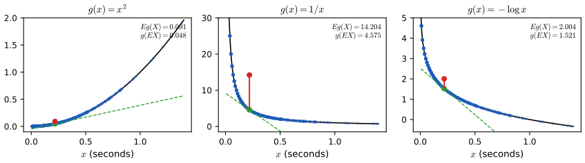
fig_4_s5. Supplementary figure; illustrates Wasserman (2004), Theorem 4.9. Download: PDF · SVGTwo applications of Jensen's inequality are used later in the book: the Kullback-Leibler divergence (consistency of maximum likelihood, Chapter 9) and the size of the largest of many normal variables (multiple testing and wavelet thresholding, Chapters 10 and 21). Both are additions to the chapter.
Definition 4.3 (Kullback-Leibler divergence)
For probability mass functions (or densities) \(p\) and \(q\), \(\KL(p,q)=\sum_xp(x)\log\frac{p(x)}{q(x)}\) (an integral for densities), the sum running over \(\{p\gt0\}\), with \(\KL(p,q)=\infty\) if \(q(x)=0\lt p(x)\) for some \(x\). For Bernoulli distributions it is the \(\kl(q,p)\) of Filling the gap 4.5.
Result 4.10 (Gibbs' inequality; not in the book)
\(\KL(p,q)\ge0\), with equality if and only if \(p=q\).
Proof
Let \(X\sim p\) and \(Y=q(X)/p(X)\), defined since \(p(X)\gt0\) almost surely. Assume \(q\gt0\) on \(\{p\gt0\}\) (otherwise \(\KL=\infty\) and there is nothing to prove). Then \(Y\gt0\), and \(\E Y=\sum_{p(x)\gt0}q(x)\le1\). Since \(-\log\) is strictly convex on \((0,\infty)\), Jensen's inequality gives
\[ \KL(p,q)=\E(-\log Y)\ge-\log\E Y=-\log\sum_{p(x)\gt0}q(x)\ge0 . \]Equality in both steps needs \(Y\) constant almost surely (strict convexity) and \(\sum_{p\gt0}q=1\); then \(Y=\E Y=1\), i.e. \(q=p\) on \(\{p\gt0\}\), and \(q\) has no mass elsewhere. ∎
The companion course proves the same with \(\log t\le t-1\) instead of Jensen: toolkit, Result T.2. On the nerve data, with \(p\) the histogram on 29 bins of width 0.05 and \(q\) an exponential model with mean \(\bar x\), \(\KL=0.0297\), of which \(-\log\E Y=0.0077\) comes from the mass (also about 0.0077) that the model puts on bins the data never visit; over the mean of the model the divergence is smallest, 0.0295, at 0.223, close to \(\bar x=0.2186\) (minimising KL from the data is maximum likelihood: Foundations of Deep Learning, Result 2.10).
Result 4.11 (the maximum of Gaussians; not in the book)
Let \(Z_1,\dots,Z_n\) be \(N(0,1)\), not necessarily independent. Then
\[ \E\max_iZ_i\le\sqrt{2\log n},\qquad\E\max_i|Z_i|\le\sqrt{2\log(2n)},\qquad\P\big(\max_i|Z_i|\gt t\big)\le n\sqrt{\frac2\pi}\frac{e^{-t^2/2}}{t}. \]Proof
Let \(M=\max_iZ_i\) and \(s\gt0\). The function \(e^{sx}\) is convex, so Jensen's inequality, then \(e^{sM}=\max_ie^{sZ_i}\le\sum_ie^{sZ_i}\), then the normal moment generating function \(\E e^{sZ}=e^{s^2/2}\) give
\[ e^{s\E M}\le\E e^{sM}\le\sum_{i=1}^n\E e^{sZ_i}=ne^{s^2/2},\qquad\text{so}\qquad\E M\le\frac{\log n}s+\frac s2 . \]The right side is smallest at \(s=\sqrt{2\log n}\), where it equals \(\sqrt{2\log n}\). For \(\max|Z_i|\), apply this to the \(2n\) variables \(\pm Z_i\). For the probability, \(\{\max|Z_i|\gt t\}=\bigcup_i\{|Z_i|\gt t\}\); the union bound and Mill's inequality finish. No independence was used. ∎
The bound \(\sqrt{2\log n}\) is the "universal threshold" of wavelet denoising (Chapter 21): with \(n\) pure-noise coefficients, essentially none exceeds it. For independent \(Z_i\) it is the correct order (Figure 4.S7).
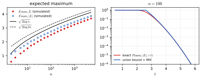
fig_4_s7. Supplementary figure; illustrates Result 4.11 (an addition to Wasserman 2004, Chapter 4). Download: PDF · SVG4.3 Bibliographic Remarks
p. 66 The book points to Devroye, Györfi and Lugosi (1996) for probability inequalities in statistics and pattern recognition, and takes its proof of Hoeffding's inequality from there. The original sources are Chernoff (1952) for the exponential (moment generating function) method and Hoeffding (1963), which also covers sampling without replacement and U-statistics. Boucheron, Lugosi and Massart (2013) is the modern reference for concentration inequalities, including Bernstein's inequality, which uses the variance as well as the range and so combines the strengths of Chebyshev's and Hoeffding's inequalities. Cover and Thomas (2006) treat the method of types used in Filling the gap 4.5.
Notes on the text (none of them is in the author's errata lists)
- p. 63, proof of Theorem 4.1. The proof begins "Since \(X\gt0\)" but the theorem assumes \(X\) non-negative, and the proof writes \(\E(X)=\int_0^\infty xf(x)\,\d x\), which needs a density. The theorem is true for every non-negative random variable; the proof above uses no density.
- p. 66, Theorem 4.8. The name is printed "Cauchy-Schwartz"; it is Hermann Amandus Schwarz, hence "Cauchy-Schwarz".
- p. 66, proof of Theorem 4.9. "Let \(L(x)=a+bx\) be a line, tangent to \(g(x)\) at the point \(\E(X)\)": a convex function need not have a tangent (\(|x|\) at 0), and the integrability of \(X\) is not stated. The proof above uses a supporting line (Filling the gap 4.8) and states the assumptions.
- p. 65, Theorem 4.7. The usual name is the Mills ratio, after J. P. Mills (1926).
The numbers in Examples 4.3 and 4.6 (0.0625 and 0.00067) and the sample size of Exercise 4(c) were confirmed numerically.
4.4 Appendix
p. 67 The proof of Hoeffding's inequality has two ingredients: a bound on the moment generating function of a single bounded, centred variable (Hoeffding's lemma), and the Chernoff method of Filling the gap 4.2, which turns such bounds for independent variables into a tail bound for their sum. The book's proof uses Taylor's theorem with the Lagrange form of the remainder: if \(g\) is twice differentiable on an interval containing 0 and \(u\), there is a \(\xi\) between 0 and \(u\) with
\[ g(u)=g(0)+ug'(0)+\frac{u^2}2g''(\xi). \]Result 4.12 (Hoeffding's lemma) p. 67, (4.9)
If \(\E(Y)=0\) and \(a\le Y\le b\), then for every real \(t\),
\[ \E\,e^{tY}\le e^{t^2(b-a)^2/8}. \]Proof
Step 1: \(a\le0\le b\). \(a\le Y\le b\) gives \(a\le\E Y=0\le b\). If \(a=b\), then \(Y=0\) and both sides are 1; assume \(a\lt b\).
Step 2: a convexity bound. Each \(y\in[a,b]\) is the convex combination \(y=\frac{y-a}{b-a}\,b+\frac{b-y}{b-a}\,a\). Since \(y\mapsto e^{ty}\) is convex,
\[ e^{tY}\le\frac{Y-a}{b-a}e^{tb}+\frac{b-Y}{b-a}e^{ta}. \]Take expectations and use \(\E Y=0\):
\[ \E\,e^{tY}\le-\frac{a}{b-a}e^{tb}+\frac{b}{b-a}e^{ta}=e^{g(u)}, \tag{4.9} \]with \(\gamma=-a/(b-a)\in[0,1]\), \(u=t(b-a)\) and \(g(u)=-\gamma u+\log(1-\gamma+\gamma e^u)\). (Check: \(b/(b-a)=1-\gamma\) and \(ta=-\gamma u\), so the middle expression is \(e^{-\gamma u}\{(1-\gamma)+\gamma e^u\}\).) The argument of the logarithm is positive because it is a weighted average of 1 and \(e^u\). The right side of (4.9) is the moment generating function of the two-point variable on \(\{a,b\}\) with mean 0: of all variables on \([a,b]\) with mean 0, this one has the largest \(\E e^{tY}\).
Step 3: \(g(u)\le u^2/8\), by the next box, for every real \(u\). Hence \(\E e^{tY}\le e^{u^2/8}=e^{t^2(b-a)^2/8}\). ∎
Filling the gap 4.10: \(g(0)=g'(0)=0\) and \(g''\le1/4\) p. 67
The book states "\(g(0)=g'(0)=0\). Also, \(g''(u)\le1/4\) for all \(u\gt0\)" without proof. In fact \(g''(u)=\rho(u)\{1-\rho(u)\}\) with \(\rho(u)=\frac{\gamma e^u}{1-\gamma+\gamma e^u}\in[0,1]\), so \(g''\le1/4\) for every real \(u\), and \(g(u)\le u^2/8\) for every real \(u\) (so the lemma also holds for \(t\lt0\), which is what the lower tail needs).
Derivation
\(g(0)=-0+\log(1-\gamma+\gamma)=0\). Differentiating,
\[ g'(u)=-\gamma+\frac{\gamma e^u}{1-\gamma+\gamma e^u}=-\gamma+\rho(u),\qquad g'(0)=-\gamma+\gamma=0. \]Next, \(1-\rho(u)=\frac{1-\gamma}{1-\gamma+\gamma e^u}\), and by the quotient rule
\[ g''(u)=\rho'(u)=\frac{\gamma e^u(1-\gamma+\gamma e^u)-\gamma e^u\cdot\gamma e^u}{(1-\gamma+\gamma e^u)^2}=\frac{\gamma e^u(1-\gamma)}{(1-\gamma+\gamma e^u)^2}=\rho(u)\{1-\rho(u)\}. \]Since \(\rho\in[0,1]\) and \(r(1-r)=\tfrac14-(r-\tfrac12)^2\le\tfrac14\), \(g''(u)\le\tfrac14\). Taylor's theorem with \(\xi\) between 0 and \(u\) (either sign of \(u\)): \(g(u)=0+0+\tfrac12u^2g''(\xi)\le u^2/8\). The probabilistic reading: \(\rho(u)\) is the probability of the upper point under the "tilted" two-point distribution, and \(g''(u)\) is its variance, never more than 1/4 for a variable on \(\{0,1\}\). ∎
For \(a=-1\), \(b=1\) (a random sign) the lemma reads \(\cosh t\le e^{t^2/2}\), which also follows by comparing the series \(\sum t^{2k}/(2k)!\) and \(\sum t^{2k}/(2^kk!)\) term by term. The constant 1/8 cannot be improved: for \(\gamma=1/2\) both sides agree to second order at \(u=0\).
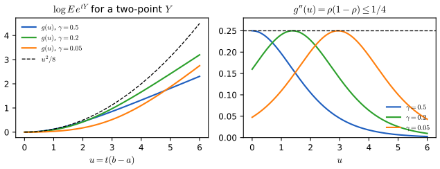
fig_4_s4. Supplementary figure; illustrates the proof in Wasserman (2004), Section 4.4. Download: PDF · SVGProof of Theorem 4.4 (the Chernoff method)
Fix \(t\gt0\). The function \(x\mapsto e^{tx}\) is increasing and positive, so by Filling the gap 4.2 (Markov's inequality applied to \(e^{t\sum Y_i}\))
\[ \P\Big(\sum_iY_i\ge\epsilon\Big)=\P\Big(e^{t\sum_iY_i}\ge e^{t\epsilon}\Big)\le e^{-t\epsilon}\,\E\,e^{t\sum_iY_i}=e^{-t\epsilon}\prod_i\E\,e^{tY_i}. \tag{4.8} \]The last step uses independence: functions of independent variables are independent, and the expectation of a product of independent integrable variables is the product of the expectations (each \(e^{tY_i}\) is bounded, hence integrable). Hoeffding's lemma (Result 4.12) bounds each factor by \(e^{t^2(b_i-a_i)^2/8}\), which is (4.3). ∎
Proof of Theorem 4.5
Let \(Y_i=(X_i-p)/n\). These are independent, \(\E Y_i=0\), and \(-p/n\le Y_i\le(1-p)/n\), an interval of length \(1/n\); so \(\sum_i(b_i-a_i)^2=1/n\). By Theorem 4.4, for every \(t\gt0\),
\[ \P(\Xbar-p\gt\epsilon)\le\P\Big(\sum_iY_i\ge\epsilon\Big)\le e^{-t\epsilon+t^2/(8n)}. \]The choice \(t=4n\epsilon\) (the minimiser, Filling the gap 4.4) gives \(e^{-4n\epsilon^2+2n\epsilon^2}=e^{-2n\epsilon^2}\). The variables \(-Y_i=(p-X_i)/n\) satisfy the same hypotheses (mean 0, range of length \(1/n\)), so \(\P(\Xbar-p\lt-\epsilon)\le e^{-2n\epsilon^2}\) as well. The event \(\{|\Xbar-p|\gt\epsilon\}\) is the union of the two disjoint events, so its probability is at most \(2e^{-2n\epsilon^2}\). ∎
4.5 Exercises
All seven exercises of Chapter 4 (Wasserman, 2004, pp. 68–69), restated in my own words, with complete solutions (hidden). The computational ones are solved with the Python code.
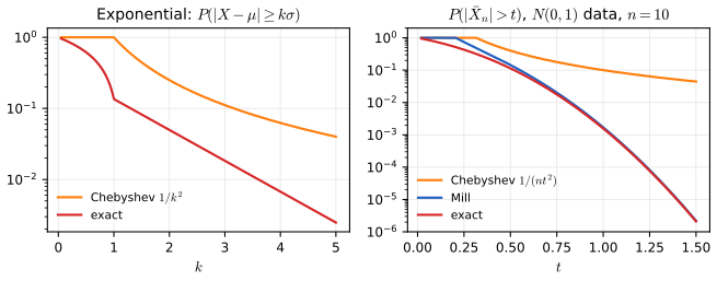
fig_4_s6. Supplementary figure; answers Wasserman (2004), Exercises 4.1 and 4.7. Download: PDF · SVGExercise 4.1. For \(X\sim\) Exponential(\(\beta\)), compute \(\P(|X-\mu_X|\ge k\sigma_X)\) for \(k\gt1\) and compare it with Chebyshev's bound.
Solution
With density \(f(x)=\beta^{-1}e^{-x/\beta}\) on \(x\gt0\), \(\mu_X=\sigma_X=\beta\) and \(\P(X\ge x)=e^{-x/\beta}\). For \(k\gt1\), the lower deviation \(X\le\beta-k\beta\lt0\) is impossible, so
\[ \P(|X-\beta|\ge k\beta)=\P\{X\ge(1+k)\beta\}=e^{-(1+k)} . \](For \(0\lt k\le1\) one adds \(\P\{X\le(1-k)\beta\}=1-e^{-(1-k)}\).) The answer does not depend on \(\beta\). Chebyshev gives \(1/k^2\): at \(k=2\), 0.0498 against 0.25; at \(k=3\), 0.0183 against 0.111; at \(k=5\), 0.0025 against 0.04. The ratio \(k^2e^{-(1+k)}\) tends to 0: the exponential tail is exponentially lighter than the worst case Chebyshev must allow (Figure 4.S6, left).
Exercise 4.2. For \(X\sim\) Poisson(\(\lambda\)), show with Chebyshev's inequality that \(\P(X\ge2\lambda)\le1/\lambda\).
Solution
\(\E X=\V(X)=\lambda\). If \(X\ge2\lambda\) then \(X-\lambda\ge\lambda\), so \(\{X\ge2\lambda\}\subseteq\{|X-\lambda|\ge\lambda\}\), and by (4.2) with \(t=\lambda\), \(\P(X\ge2\lambda)\le\lambda/\lambda^2=1/\lambda\). For \(\lambda=10\) the bound is 0.1 and the exact value \(\P(X\ge20)\) is 0.0035. Cantelli's one-sided form (Filling the gap 4.3) improves the bound to \(\lambda/(\lambda+\lambda^2)=1/(1+\lambda)\).
Exercise 4.3. For \(X_1,\dots,X_n\sim\) Bernoulli(\(p\)), bound \(\P(|\Xbar-p|\gt\epsilon)\) with Chebyshev's and with Hoeffding's inequality, and show that Hoeffding's bound is the smaller one when \(n\) is large.
Solution
Chebyshev (Example 4.3): \(\frac{p(1-p)}{n\epsilon^2}\le\frac1{4n\epsilon^2}\). Hoeffding (Theorem 4.5): \(2e^{-2n\epsilon^2}\). Their ratio is
\[ \frac{2e^{-2n\epsilon^2}}{p(1-p)/(n\epsilon^2)}=\frac{2x\,e^{-2x}}{p(1-p)},\qquad x=n\epsilon^2, \]which tends to 0 as \(n\to\infty\) for fixed \(p\in(0,1)\) and \(\epsilon\), because \(xe^{-2x}\to0\). So for all large \(n\) Hoeffding's bound is smaller, and by an exponentially growing factor. Against the \(p\)-free form \(1/(4n\epsilon^2)\), Hoeffding is smaller exactly when \(8xe^{-2x}\lt1\), i.e. for \(x\gt1.0766\) (and for \(x\lt0.1787\), where both bounds exceed 1); for \(\epsilon=0.2\) this means \(n\ge27\). When \(p\) is small, how large "large" is depends on \(p\): for \(p=\epsilon=0.05\), Chebyshev's bound with the true variance is smaller up to \(n=913\) (Figure 4.S1(c)).
Exercise 4.4. For \(X_1,\dots,X_n\sim\) Bernoulli(\(p\)), \(\alpha\gt0\) and \(\epsilon_n=\sqrt{\log(2/\alpha)/(2n)}\), let \(C_n=(\hat p_n-\epsilon_n,\hat p_n+\epsilon_n)\) with \(\hat p_n=\Xbar\). (a) Show that \(\P(p\in C_n)\ge1-\alpha\). (b) Computer experiment: with \(\alpha=0.05\) and \(p=0.4\), estimate the coverage by simulation for \(n\) between 1 and 10,000, and plot it against \(n\). (c) Plot the length of the interval against \(n\); how large must \(n\) be for the length to be at most 0.05?
Solution
(a) \(\P(p\notin C_n)=\P(|\hat p_n-p|\ge\epsilon_n)\le2e^{-2n\epsilon_n^2}=\alpha\) by Theorem 4.5 (the "\(\ge\)" is covered by applying (4.4) with \(\epsilon\uparrow\epsilon_n\) and using continuity from above of \(\P\)). Truncating to \([0,1]\) does not change whether \(p\in C_n\) (Filling the gap 4.6(b)).
(b) Method:
coverage_simdraws 1000 data sets of \(n\) Bernoulli(0.4) observations at each of 13 sample sizes from 1 to 10,000 and records how often \(C_n\) contains 0.4;coverage_exactcomputes the coverage exactly as \(\sum_k\binom nk p^k(1-p)^{n-k}\ind\{|k/n-p|\lt\epsilon_n\}\) on 200 sample sizes. Result (Figure 4.S2, left): the coverage is between 0.9926 and 1 for every \(n\) (for \(n=1,2\), \(\epsilon_n\gt0.6\) and the interval always contains 0.4), far above the nominal 0.95, settling near the limit 0.9944 of Filling the gap 4.6(e); the simulated values agree with the exact ones to within simulation error (e.g. 0.992 against 0.9944 at \(n=100\)). The normal-approximation interval, shown for comparison, covers only 0.90 at \(n=10\) and 0.93 to 0.95 between \(n=20\) and 100, oscillating as \(n\) changes.(c) The length is \(2\epsilon_n=\sqrt{2\log 40/n}\), a straight line of slope \(-1/2\) on log-log axes (Figure 4.S2, right). \(2\epsilon_n\le0.05\iff n\ge2\log 40/0.05^2=2951.1\), so \(n=2952\). (Truncation shortens the interval only when it overlaps 0 or 1; at \(p=0.4\) the mean truncated length is within 1% of \(2\epsilon_n\) from \(n=25\) on.) The normal interval would reach length 0.05 at about \(n=1475\): the guaranteed coverage costs a factor of about 2 in sample size.
Exercise 4.5. Prove Mill's inequality (Theorem 4.7). Hint: \(\P(|Z|\gt t)=2\P(Z\gt t)\), and \(x/t\gt1\) when \(x\gt t\).
Solution
\(\P(Z\gt t)=\int_t^\infty\phi(x)\,\d x\le\int_t^\infty\frac xt\phi(x)\,\d x=\frac1t\int_t^\infty x\phi(x)\,\d x=\frac{\phi(t)}t\), since \(x\phi(x)=-\phi'(x)\). Doubling, \(\P(|Z|\gt t)\le\frac{2}{t\sqrt{2\pi}}e^{-t^2/2}=\sqrt{\frac2\pi}\frac{e^{-t^2/2}}t\). The full proof, with the matching lower bound, is under Theorem 4.7.
Exercise 4.6. For \(Z\sim N(0,1)\), compute \(\P(|Z|\gt t)\) and plot it against \(t\). Markov's inequality gives \(\P(|Z|\gt t)\le\E|Z|^k/t^k\) for every \(k\gt0\); plot these bounds for \(k=1,\dots,5\) and compare them with the truth, and also plot Mill's bound.
Solution
\(\P(|Z|\gt t)=2\{1-\Phi(t)\}=\operatorname{erfc}(t/\sqrt2)\). The moments are \(\E|Z|=\sqrt{2/\pi}=0.798\), \(\E Z^2=1\), \(\E|Z|^3=2\sqrt{2/\pi}=1.596\), \(\E Z^4=3\), \(\E|Z|^5=8\sqrt{2/\pi}=6.383\) (Filling the gap 4.7(a)). Figure 4.S3 shows the result. Findings: (i) every bound is valid but polynomial in \(t\), while the truth decays like \(e^{-t^2/2}\); (ii) the bounds cross: higher \(k\) is better for larger \(t\) (by Lyapunov's inequality, the \(k\)-th root of the \(k\)-th moment grows with \(k\)); at \(t=3\), \(k=1,\dots,5\) give 0.27, 0.11, 0.059, 0.037, 0.026, against the truth 0.0027, and even the best real order (\(k\approx9\)) gives only 0.0156; (iii) Mill's bound is above 1 for small \(t\), useless there, but within 20% of the truth from \(t=2\) and within 10% from \(t=3\).
Exercise 4.7. For \(X_1,\dots,X_n\sim N(0,1)\), bound \(\P(|\Xbar|\gt t)\) with Mill's inequality and compare with the Chebyshev bound.
Solution
A sum of independent normals is normal, so \(\Xbar\sim N(0,1/n)\) and \(\sqrt n\,\Xbar\sim N(0,1)\). With \(s=\sqrt n\,t\),
\[ \P(|\Xbar|\gt t)=\P(|Z|\gt s)\le\sqrt{\frac2\pi}\,\frac{e^{-nt^2/2}}{\sqrt n\,t}\quad\text{(Mill)},\qquad\P(|\Xbar|\gt t)\le\frac{1}{nt^2}\quad\text{(Chebyshev)}. \]The ratio Mill/Chebyshev is \(\sqrt{2/\pi}\,s\,e^{-s^2/2}\), whose maximum over \(s\gt0\) (at \(s=1\)) is \(\sqrt{2/\pi}\,e^{-1/2}=0.484\). So Mill's bound is always less than half of Chebyshev's, and for fixed \(t\) it is smaller by the factor \(\sqrt n\,t\,e^{-nt^2/2}\to0\) as \(n\) grows (Figure 4.S6, right, for \(n=10\)).
Demonstrations for this chapter
Each demonstration runs in the browser, with exact computations and seeded random numbers, and links back to these notes. The ▶ Demo boxes above open them already set to the case under discussion. The numbers they show are the same as those of the Python code.
| Demonstration | What you can see | Sections and results |
|---|---|---|
| Markov, Chebyshev, Hoeffding and the exact tail | The exact tail of a binomial proportion against every bound, as functions of \(\epsilon\) and of \(n\) on a log scale; the normal tail against the moment bounds, Chernoff and Mill. Presets: 1 Examples 4.3 and 4.6; 2 small \(p\); 3 Markov attained; 4 large \(n\); 5 Exercise 6. | 4.1; Theorems 4.1, 4.2, 4.5, 4.7; gap 4.5 |
| Hoeffding's interval for a proportion | Simulated intervals, exact coverage and expected length against \(n\) for Hoeffding's and the normal interval, and the sample size for a target length. Presets: 1 Exercise 4(b); 2 Exercise 4(c); 3 small \(n\); 4 rare event; 5 \(\alpha=0.01\). | Definition 4.1, gap 4.6, Exercise 4 |
| Jensen's inequality | Six convex functions on two-point distributions and on the nerve data, with the supporting line and the gap; the KL divergence between the nerve histogram and an exponential model as a Jensen gap. Presets: 1 the gap is a variance; 2 AM and GM; 3 the harmonic mean; 4 a corner; 5 KL. | 4.2; gap 4.8, Theorem 4.9, gap 4.9, Result 4.10 |
The Python code that produces every figure of this page is code/ch04_inequalities.py (see the code index).
References
- Wasserman, L. (2004). All of Statistics: A Concise Course in Statistical Inference. Springer, New York. Chapter 4, pp. 63–69. www.stat.cmu.edu/~larry/all-of-statistics.
- Boucheron, S., Lugosi, G. and Massart, P. (2013). Concentration Inequalities: A Nonasymptotic Theory of Independence. Oxford University Press.
- Brown, L. D., Cai, T. T. and DasGupta, A. (2001). Interval estimation for a binomial proportion. Statistical Science, 16(2), 101–133.
- Chernoff, H. (1952). A measure of asymptotic efficiency for tests of a hypothesis based on the sum of observations. Annals of Mathematical Statistics, 23(4), 493–507.
- Cover, T. M. and Thomas, J. A. (2006). Elements of Information Theory, 2nd edition. Wiley, Hoboken.
- Devroye, L., Györfi, L. and Lugosi, G. (1996). A Probabilistic Theory of Pattern Recognition. Springer, New York.
- Hoeffding, W. (1963). Probability inequalities for sums of bounded random variables. Journal of the American Statistical Association, 58(301), 13–30. doi:10.1080/01621459.1963.10500830.
- Mills, J. P. (1926). Table of the ratio: area to bounding ordinate, for any portion of normal curve. Biometrika, 18(3/4), 395–400.
The numerical statements in the text (the exact tails and every bound, the Chernoff exponent and its lower bound, the coverage and lengths of both intervals, Mill's bounds and the normal moments, the nerve-data means and divergences, and the Gaussian maxima) were confirmed numerically.