Recommender Systems
A recommender system predicts which items a user will like from the history of what users did with items: the data are the entries of a huge, mostly empty user-by-item table. The chapter builds up from similarity-based collaborative filtering to low-rank matrix factorisation (the model that won the Netflix competition's core), its probabilistic reading and a neural variant, then to learning from clicks alone (implicit feedback, with a ranking loss), to models that accept side information (factorisation machines, which also solve the cold-start problem), and finally to the feedback loop that makes recommendation different from ordinary prediction: the system only sees the clicks on what it chose to show, so it must explore. Because MovieLens and Netflix are not available offline, every figure here is computed on a simulated ratings matrix with a known low-rank structure, which also lets us check each method against the truth.
Ch. 1 Introduction Ch. 2 Univariate probability Ch. 3 Multivariate probability Ch. 4 Statistics Ch. 5 Decision theory Ch. 6 Information theory Ch. 7 Linear algebra Ch. 8 Optimisation Ch. 9 Discriminant analysis Ch. 10 Logistic regression Ch. 11 Linear regression Ch. 12 GLMs Ch. 13 Networks for tabular data Ch. 14 Networks for images Ch. 15 Networks for sequences Ch. 16 Exemplar-based methods Ch. 17 Kernel methods Ch. 18 Trees and boosting Ch. 19 Fewer labels Ch. 20 Dimensionality reduction Ch. 21 Clustering Ch. 22 Recommender systems Ch. 23 Graph embeddings
How to read these notes
They follow the book. Sections carry the book's numbers (22.1.3.1, 22.2.2, ...) and equations the book numbers keep their numbers, e.g. \((22.4)\); equations without a number are steps the book skips. The chapter is short and descriptive (it has no end-of-chapter exercises), so most of the work here is to supply what a reader needs to use the methods: the derivations the book omits, the corrections it needs, and a quantitative look at each method on data with known structure.
Filling the gaps. Wherever the book writes a result without a proof, or leaves a step out, an orange Filling the gap box gives the full argument. Proofs start hidden: open one with its bar, or use the buttons below.
Figures and demonstrations. Every computed figure is reproduced by the Python code, written from scratch (alternating least squares, stochastic gradient descent, the zero-filled SVD, Bayesian personalised ranking, factorisation machines, bandit policies, inverse propensity weighting). Figure 22.5 is a hand-drawn network diagram and is not reproduced. Figures 22.2 to 22.4 are drawn on a simulated ratings matrix (the book's own come from Netflix and MovieLens), so items are labelled by simulated genre rather than by movie title; the supplementary figures S1 to S8 illustrate the gaps.
Main reference
K. P. Murphy, Probabilistic Machine Learning: An Introduction, MIT Press (2022), Chapter 22, pages 741–751 (book page: probml.github.io/pml-book/book1.html). Section, equation and figure numbers below refer to this book. The explanations, derivations, figures and code are my own.
Companion courses
Recommenders are built from ideas developed in other courses on this site. Where a result is proved in full there, these notes give the statement and a short sketch and link to it.
- Bayesian and Probabilistic Machine Learning (Bishop): 12.1.2 PCA as minimum-error projection (the fully observed matrix-factorisation problem), 3.1.4 regularised least squares (each half-step of alternating least squares), 4.3 logistic regression (the model inside the ranking loss), and the conjugate updating demonstration (the Beta posterior of Thompson sampling).
- Elements of Statistical Learning (Hastie, Tibshirani, Friedman): 14.5.1 principal components and 14.6 non-negative matrix factorisation.
- Introduction to Statistical Learning (James, Witten, Hastie, Tibshirani): 12.3 missing values and matrix completion (the iterative low-rank imputation, which is the soft-impute relative of the model here).
- Foundations of Deep Learning (Bishop and Bishop): 7.2.3 stochastic gradient descent and 19.1 deterministic autoencoders (AutoRec).
- Earlier chapters of this course: 7.5.5 truncated SVD (Eckart-Young), 8.4 stochastic gradient descent, 11.3 ridge regression, 10.2.4 SGD for logistic regression, 4.5.1 MAP estimation as regularisation.
What this chapter adds: the observed-entries-only objective and its non-identifiability, the exact alternating least squares half-steps and a nuclear-norm view of the penalty, the bias of the zero-filled SVD, informative missingness and inverse propensity weighting, ranking losses and their link to the AUC, the factorisation machine identity (with a sign correction), cold start, and regret and logged-data evaluation for the feedback loop.
The chapter at a glance
- 22.1 Explicit ratings form a sparse matrix. Missing at random is an assumption (gap 22.1). Neighbourhood methods need a normalisation (gap 22.2). Matrix completion is under-determined, non-convex and defined up to a rotation (gap 22.3); alternating least squares (gap 22.4) and SGD (gap 22.5) fit the biased factorisation; PMF is its MAP reading (gap 22.6); the zero-filled SVD of the MovieLens example shrinks all predictions (gap 22.7); AutoRec (gap 22.8).
- 22.2 Implicit feedback needs a ranking loss: Bayesian personalised ranking (gap 22.9); factorisation machines and their linear-time identity (gap 22.10); neural matrix factorisation (gap 22.11).
- 22.3 Side information and cold start (gap 22.12).
- 22.4 The feedback loop: regret of greedy, ε-greedy, UCB1 and Thompson sampling (gap 22.13) and evaluating a new policy on logged data (gap 22.14).
Notation. \(M\) users, \(N\) items, \(Y_{ui}\) the rating of user \(u\) for item \(i\), \(\Obs\) the set of observed pairs \((u,i)\), \(n_u\) and \(m_i\) the number of ratings of user \(u\) and of item \(i\). \(\bm U\in\R^{M\times K}\) and \(\bm V\in\R^{N\times K}\) have rows \(\bm u_u\) and \(\bm v_i\); \(\mu\) is the global mean, \(b_u\) and \(c_i\) are user and item offsets, \(\hat y_{ui}\) the prediction, \(e_{ui}=y_{ui}-\hat y_{ui}\) the error, \(\lambda\) a penalty, \(\eta\) a step size. \(\sigma(a)=1/(1+e^{-a})\) is the logistic function; \(\|\cdot\|_F\) the Frobenius norm.
Prerequisites. Linear least squares and ridge regression (Chapter 11), the SVD (Section 7.5), stochastic gradient descent (Section 8.4), logistic regression (Chapter 10), MAP estimation (Section 4.5), the beta-binomial model (Section 4.6.2).
22.1 Explicit feedback
p. 741 In the simplest setting each user gives an explicit score, a rating from 1 to 5 or a like/dislike, to some of the items. Let \(Y_{ui}\) be the rating of user \(u\) for item \(i\). Collect these in an \(M\times N\) matrix \(\bm Y\) that is very large and very sparse: most users rate a tiny fraction of the items. The same data are a bipartite graph with an edge of weight \(Y_{ui}\) between user \(u\) and item \(i\) wherever a rating exists; because the labels \(u\) and \(i\) are arbitrary indices, what carries information is only who is connected to whom (relational data). Figure 22.1 shows a toy example: users 3 and 4 give similar ratings, so user 3's ratings help predict user 4's; user 1 rates everything low; user 2 has too little data for a reliable prediction.
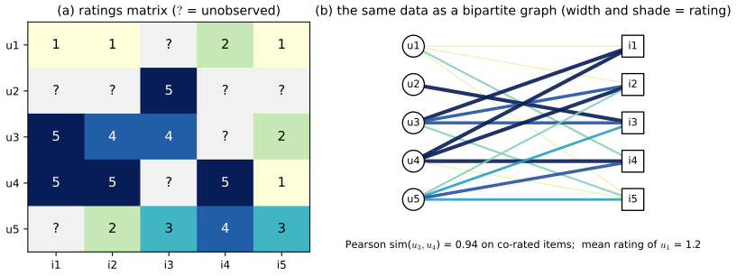
A missing entry can mean that user \(u\) never encountered item \(i\), or that they saw it and chose not to engage because they expected not to like it. In the first case the missingness carries no information about \(Y_{ui}\); in the second it does. The book assumes the first (data are missing at random), and so do all the methods below; gap 22.1 shows what goes wrong otherwise and how to correct for it when the observation probabilities are known.
Filling the gap 22.1: missing at random, informative missingness and inverse propensity weighting p. 741
Derivation
Setup. Let \(Y_{ui}\) be the (latent) rating of every pair and \(O_{ui}\in\{0,1\}\) indicate whether it is observed, with propensity \(P_{ui}=\Pr(O_{ui}=1\mid Y_{ui},\text{covariates})\). The data are \(\{(u,i,Y_{ui}):O_{ui}=1\}\). The mechanism is missing at random (here: missing completely at random given user and item) if \(P_{ui}\) does not depend on \(Y_{ui}\). Then the likelihood of the observed entries factorises into a part for the ratings and a part for the mechanism, the second does not involve the rating parameters, and ignoring it is valid (Rubin, 1976): fitting a model to the observed entries only is correct. If \(P_{ui}\) depends on \(Y_{ui}\) (missing not at random), the observed entries are a biased sample.
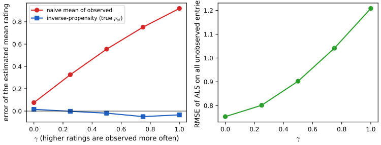
The bias, in an example. Let a rating have pmf \(p(r)\), \(r\in\{1,\dots,5\}\), and be observed with probability proportional to \(e^{\gamma(r-3)}\), \(\gamma>0\) (users rate what they like). The observed ratings have the exponentially tilted pmf \(p_\gamma(r)=p(r)e^{\gamma(r-3)}/Z(\gamma)\), with mean \[ m(\gamma)=\E_\gamma[Y]=\frac{\d}{\d\gamma}\log Z(\gamma)\ (+3),\qquad m'(\gamma)=\var_\gamma(Y)\ge0 , \] because \(\log Z\) is a cumulant generating function (its second derivative is the variance). So \(m(\gamma)\ge m(0)=\E[Y]\): the mean of the observed ratings overestimates the population mean, and the error grows with \(\gamma\). In the simulation of Figure 22.S4 (300 users, 200 items, 12 percent observed) the error of the naive mean is 0.08, 0.56 and 0.92 rating points for \(\gamma=0,\,0.5,\,1\), and a factorisation fitted to the observed entries predicts the unobserved entries worse and worse (RMSE 0.75, 0.90, 1.21).
Inverse propensity weighting. If the propensities are known (or well estimated), the Horvitz-Thompson trick removes the bias: since \(\E[O_{ui}Y_{ui}/P_{ui}]=P_{ui}Y_{ui}/P_{ui}=Y_{ui}\), the sum \(\sum_{(u,i)\in\Obs}Y_{ui}/P_{ui}\) is an unbiased estimate of the sum of all \(MN\) ratings, and the self-normalised ratio \(\sum_\Obs Y_{ui}/P_{ui}\big/\sum_\Obs1/P_{ui}\) (consistent, slightly biased in finite samples, much lower variance) estimates the population mean. In the simulation its error is 0.02, \(-0.02\) and \(-0.03\) for the three values of \(\gamma\). The same weights can multiply each squared error in (22.5) to fit a factorisation to the full population (Schnabel et al., 2016). Estimating the propensities is the hard part in practice. Marlin et al. (2011), cited by the book, study this on real ratings.
22.1.1 Datasets
pp. 741–742 The Netflix Prize data (2006) held 100,480,507 ratings from 480,189 users on 17,770 movies; the fraction of the \(480{,}189\times17{,}770\) matrix that is observed is only \(1.18\%\), so the matrix is \(98.8\%\) empty ("99 percent sparse", as the book says). The data have been withdrawn for privacy reasons. MovieLens-1M (6,040 users, 3,706 movies, 1,000,209 ratings) is observed in \(4.47\%\) of its entries; the average movie has 270 ratings but the average user only 166, which matters for the choice between item-based and user-based AutoRec (gap 22.8). Other public sets are the Jester jokes and BookCrossing data.
These data are not available offline, so the notes use a simulated matrix with the same structure: \(M=300\) users and \(N=200\) items in six genres; the rating before rounding is \(\mu+b_u+c_i+\bm u_u^\T\bm v_i\) plus Gaussian noise of standard deviation 0.5, with a true latent dimension of 3, \(\mu=3.4\), user and item offsets of standard deviation 0.35 and 0.4, rounded and clipped to \(\{1,\dots,5\}\). Entries are observed with probability proportional to a user activity times an item popularity, 12 percent in all (7,191 ratings, 24 per user and 36 per item on average), and 20 percent of the observed ratings are held out for testing. Because the true mean rating of every entry is known, the best conceivable test RMSE is known too: 0.576, the error of the true mean against the held-out ratings.
22.1.2 Collaborative filtering
p. 742 The original approach, collaborative filtering, lets users "collaborate" by sharing ratings: to predict whether \(u\) will like \(i\), look at the ratings that similar users \(u'\) gave to \(i\) and take a weighted average, \[ \hat Y_{ui}=\sum_{u':Y_{u'i}\neq?}\operatorname{sim}(u,u')\,Y_{u'i} . \tag{22.1} \] Similarity was traditionally computed by comparing the sets of items the two users rated; with sparse data two users share few items and the similarity is noisy. Gap 22.2 adds the normalisation that (22.1) needs to be an average at all, and the mean-centring that makes it work.
Filling the gap 22.2: (22.1) as a normalised weighted average, mean-centring, and what sparsity does to the similarity p. 742, (22.1)
Derivation
(22.1) is not an average. A weighted average has weights summing to one. If \(n\) neighbours all have similarity 1 and rate item \(i\) with 4, (22.1) returns \(4n\): the prediction grows with the number of raters of \(i\) and leaves the rating scale. The fix is to divide by the total weight, \[ \hat Y_{ui}=\frac{\sum_{u'}s_{uu'}Y_{u'i}}{\sum_{u'}|s_{uu'}|},\qquad s_{uu'}=\operatorname{sim}(u,u'). \] For nonnegative weights this is the minimiser over \(a\) of the weighted squared error \(\sum_{u'}s_{uu'}(Y_{u'i}-a)^2\) (set the derivative \(-2\sum s_{uu'}(Y_{u'i}-a)\) to zero), i.e. a Nadaraya-Watson kernel regression over users, with the similarity as the kernel.
Mean-centring. Some users rate high and some low. Replacing \(Y_{u'i}\) by \(Y_{u'i}-\bar Y_{u'}\) (the neighbour's own mean) and adding back \(\bar Y_u\), \[ \hat Y_{ui}=\bar Y_u+\frac{\sum_{u'}s_{uu'}\,(Y_{u'i}-\bar Y_{u'})}{\sum_{u'}|s_{uu'}|}, \] predicts how far above or below their own average user \(u\) will rate the item, which is what similar users agree on. A natural similarity is then the cosine of the mean-centred rating vectors on the items both users rated (the Pearson correlation if the means are taken on those items). Because two users share few items in a sparse matrix, the cosine is computed from few terms; the code shrinks it by \(n_{uu'}/(n_{uu'}+5)\) where \(n_{uu'}\) is the number of shared items, and keeps the 20 most similar users who rated \(i\).
Item-based version. Exchanging the roles of users and items (similar items, the same user's ratings) gives item-based filtering, usually cheaper when there are fewer items than users and with more stable similarities when items have more ratings than users (compare the 270 and 166 of MovieLens-1M).
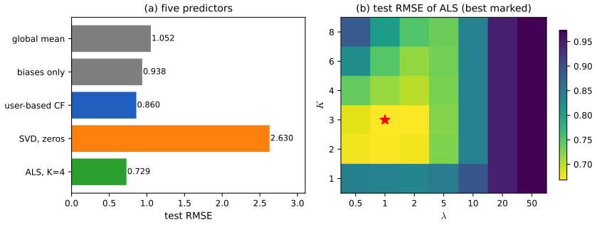
Result. On the simulated data the test RMSE is 1.052 for the global mean, 0.938 for a model with only user and item offsets, 0.860 for the user-based estimator above, and 0.729 for a matrix factorisation (Figure 22.S1a). Neighbourhood methods exploit the same structure but use it indirectly and only from pairs of users with enough overlap; a factorisation shares strength through the learned dense vectors, the book's remark at the end of Section 22.1.2.
22.1.3 Matrix factorization
p. 743 View the task as matrix completion: fill in the missing entries of \(\bm Y\). Minimising \(L(\bm Z)=\sum_{ij:Y_{ij}\neq?}(Z_{ij}-Y_{ij})^2\) over matrices \(\bm Z\) (22.2) is under-specified, since any \(\bm Z\) that agrees with \(\bm Y\) on the observed entries has zero loss. A constraint is needed: assume \(\bm Y\) has low rank, \(\bm Z=\bm U\bm V^\T\) with \(K\) columns in each factor, so that \[ \hat y_{ui}=\bm u_u^\T\bm v_i \tag{22.3} \] (matrix factorisation: user \(u\) and item \(i\) get \(K\)-dimensional vectors, and the prediction is their inner product). If every entry is observed the optimum is the truncated SVD (Section 7.5.5); with missing entries the problem is not convex and the solution is not unique (gap 22.3). Two practical fitting methods are alternating least squares (gap 22.4), where one estimates \(\bm U\) given \(\bm V\) and then \(\bm V\) given \(\bm U\), and stochastic gradient descent (gap 22.5). In practice one adds baselines, \[ \hat y_{ui}=\mu+b_u+c_i+\bm u_u^\T\bm v_i , \tag{22.4} \] so that the factors need not explain that some users rate high and some items are popular, and an \(\ell_2\) penalty: \[ L(\bm\theta)=\sum_{(u,i)\in\Obs}(y_{ui}-\hat y_{ui})^2+\lambda\big(b_u^2+c_i^2+\|\bm u_u\|^2+\|\bm v_i\|^2\big). \tag{22.5} \]
Filling the gap 22.3: why completion is under-determined, non-convex and identified only up to a rotation; the fully observed case p. 743, (22.2)–(22.3)
Derivation
(22.2) is a masked norm. The sum runs over the observed entries only, so \(L(\bm Z)=\|P_\Obs(\bm Z-\bm Y)\|_F^2\) with \(P_\Obs\) zeroing the unobserved entries; it equals \(\|\bm Z-\bm Y\|_F^2\) only when every entry is observed. Every \(\bm Z\) agreeing with \(\bm Y\) on \(\Obs\) has \(L=0\), which is why a constraint is required.
Fully observed case: the truncated SVD is optimal (Eckart-Young-Mirsky). Let \(\bm Y\) have singular values \(\sigma_1\ge\sigma_2\ge\cdots\). For every \(\bm Z\) of rank at most \(K\), \[ \|\bm Y-\bm Z\|_F^2\ \ge\ \sum_{k>K}\sigma_k(\bm Y)^2 , \] with equality for \(\bm Z=\sum_{k\le K}\sigma_k\bm p_k\bm q_k^\T\), the truncated SVD. Proof. Weyl's inequality for singular values, \(\sigma_{i+j-1}(\bm A+\bm B)\le\sigma_i(\bm A)+\sigma_j(\bm B)\), applied to \(\bm Y=\bm Z+(\bm Y-\bm Z)\) with \(i=K+1\) and \(j=k\) gives \(\sigma_{K+k}(\bm Y)\le\sigma_{K+1}(\bm Z)+\sigma_k(\bm Y-\bm Z)=\sigma_k(\bm Y-\bm Z)\), because \(\operatorname{rank}\bm Z\le K\) forces \(\sigma_{K+1}(\bm Z)=0\). Squaring and summing over \(k\ge1\) and using \(\|\bm A\|_F^2=\sum_k\sigma_k(\bm A)^2\) gives the bound. \(\square\) This is the book's Section 7.5.5 and, in statistical language, PCA (companion course, 12.1.2).
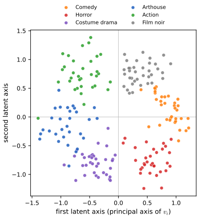
Non-identifiability. For any invertible \(K\times K\) matrix \(\bm A\), \(\bm U\bm V^\T=(\bm U\bm A)(\bm V\bm A^{-\T})^\T\), so the objective (22.2) is constant along the whole orbit of \((\bm U,\bm V)\). With the penalty in (22.5) the orbit shrinks to \(\bm A\) orthogonal (rotations and reflections), because then \(\|\bm U\bm A\|_F=\|\bm U\|_F\) and \(\|\bm V\bm A^{-\T}\|_F=\|\bm V\|_F\) (and one can show these are the only transformations that leave the penalty unchanged for generic \(\bm U,\bm V\)). Consequently the individual latent axes of Figure 22.2 have no intrinsic meaning: only distances and inner products among the vectors do. That is why our Figure 22.2 shows the item vectors on their principal axes.
Non-convexity, even without missing data. The book says that with missing entries the objective "is no longer convex", which suggests it is convex when everything is observed; it is not. Take \(f(\bm U,\bm V)=\|\bm Y-\bm U\bm V^\T\|_F^2\) with \(\bm Y\ne0\) and a global minimiser \((\bm U^*,\bm V^*)\) with \(\bm U^*\bm V^{*\T}\ne0\) (so \(f^*<\|\bm Y\|_F^2\)). Then \((-\bm U^*,-\bm V^*)\) has the same value \(f^*\), and the midpoint \((\bm 0,\bm 0)\) has value \(\|\bm Y\|_F^2>f^*\), contradicting convexity (\(f(\text{midpoint})\le\frac12(f^*+f^*)\)). The numerical experiment on the simulated matrix with penalty \(\lambda=5\): \(f(\bm 0,\bm 0)=4843\) against the converged value 3579. What the missing entries add is the possibility of spurious local minima: for the weighted problem (weight 0 on missing entries) local minima that are not global exist (Srebro and Jaakkola, 2003, the book's [SJ03]), whereas for the fully observed problem all local minima are global and the other critical points are saddles.
A pattern with infinitely many solutions. If the observed entries are \(Y_{11}=Y_{22}=1\) only, then every rank-one matrix \(\bigl[\begin{smallmatrix}1&a\\1/a&1\end{smallmatrix}\bigr]\), \(a\neq0\), fits them exactly: the rank constraint alone does not determine the missing entries when the observation pattern is poorly connected (a "disconnected" bipartite graph). This is the user 2 of Figure 22.1: with one observation there is nothing to compare.
Filling the gap 22.4: alternating least squares, derived; monotone decrease, convergence, the penalty reading, and a nuclear-norm view p. 743, (22.4)–(22.5)
Derivation
Each half-step is a ridge regression. Fix \(\mu\) (the mean of the training ratings), all \(c_i\) and all \(\bm v_i\), and write \(\bm\theta_u=(b_u,\bm u_u)\in\R^{K+1}\). The terms of (22.5) that involve user \(u\) are, with \(I_u=\{i:(u,i)\in\Obs\}\), \[ \sum_{i\in I_u}\big(t_{ui}-\bm z_i^\T\bm\theta_u\big)^2+\lambda\|\bm\theta_u\|^2,\qquad \bm z_i=(1,\bm v_i),\quad t_{ui}=y_{ui}-\mu-c_i . \] This is a ridge regression (Section 11.3) with design matrix \(\bm Z_u\) (rows \(\bm z_i^\T\)): strictly convex for \(\lambda>0\), with unique minimiser \[ \hat{\bm\theta}_u=\big(\bm Z_u^\T\bm Z_u+\lambda\bm I\big)^{-1}\bm Z_u^\T\bm t_u . \] The item step is the same with the roles exchanged. A user with no ratings gets \(\bm\theta_u=\bm0\). One full iteration costs \(O(|\Obs|K^2+(M+N)K^3)\): form the \((K+1)\times(K+1)\) Gram matrix of each user or item from its own ratings, and solve. The problems for different users are independent, so the half-step parallelises.
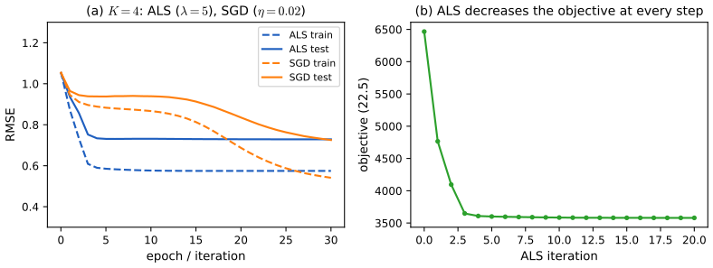
Monotone decrease and convergence. Each half-step minimises (22.5) exactly over one block with the other fixed, so it cannot increase the objective, and the objective is bounded below by 0. Hence the objective values converge (Figure 22.S2b: from 6466 to 3579 in 20 iterations, with almost all of the decrease in the first four iterations). Because the objective is coercive for \(\lambda>0\) (level sets are bounded) and each block minimiser is unique, every limit point of the iterates is a stationary point of (22.5) (Bertsekas, 1999, block coordinate descent with unique block minima). Stationarity is all one can claim: the problem is non-convex (gap 22.3) and the limit depends on the initialisation. Note that \(\bm U=\bm V=\bm 0\) is itself a stationary point of (22.5) (all gradients with respect to the factors vanish there), so \(\bm V\) must start at small random values, not at zero; the demonstration uses fixed random numbers of standard deviation 0.1.
Which penalty? Read literally, (22.5) places the penalty inside the sum over observed pairs, so user \(u\)'s parameters are penalised \(n_u\) times: \(\lambda n_u(b_u^2+\|\bm u_u\|^2)\). This is what stochastic gradient descent on one observation at a time optimises (gap 22.5). The alternating least squares above (and the demonstration and code) use the plain ridge version in which each parameter is penalised once with strength \(\lambda\). The two differ by a user- and item-dependent rescaling of \(\lambda\) (heavy raters are shrunk more in the first), and the optimal \(\lambda\) differs.
A nuclear-norm view of the penalty (fully observed, no baselines). For \(\bm Z=\bm U\bm V^\T\) one has \(\min_{\bm U\bm V^\T=\bm Z}\big(\|\bm U\|_F^2+\|\bm V\|_F^2\big)=2\|\bm Z\|_*\), where \(\|\bm Z\|_*=\sum_k\sigma_k(\bm Z)\) is the nuclear norm (attained by the balanced factorisation \(\bm U=\bm P\bm S^{1/2},\bm V=\bm Q\bm S^{1/2}\); the inequality follows from \(2\|\bm Z\|_*=2\operatorname{tr}(\bm S)\le\|\bm U\|_F^2+\|\bm V\|_F^2\) by the trace inequality for the SVD). So with all entries observed and \(K\) at least the rank of the answer, minimising \(\|\bm R-\bm U\bm V^\T\|_F^2+\lambda(\|\bm U\|_F^2+\|\bm V\|_F^2)\) is minimising \(\|\bm R-\bm Z\|_F^2+2\lambda\|\bm Z\|_*\), which separates over the singular values of \(\bm R\) as \((\sigma_k-z_k)^2+2\lambda z_k\), minimised by \[ \hat{\bm Z}=\sum_k(\sigma_k(\bm R)-\lambda)_+\,\bm p_k\bm q_k^\T :\] the ridge penalty on the factors soft-thresholds the singular values at \(\lambda\) and sets all factors with \(\sigma_k\le\lambda\) to zero. This was confirmed numerically (ridge ALS with \(K=8\), no baselines, on the fully observed simulated matrix with \(\lambda=40\) agrees with the soft-thresholded SVD to \(10^{-14}\); five singular values exceed 40). It explains why too large a \(\lambda\) collapses the model to the baselines (Figure 22.S1b, \(\lambda\ge20\); demonstration preset 5), and it is the complete-data version of the convex soft-impute method (Mazumder, Hastie and Tibshirani, 2010; ISL 12.3) for missing entries.
Filling the gap 22.5: the stochastic gradient updates (22.6)–(22.9) p. 743
Derivation
Sample one observed pair \((u,i)\) uniformly from \(\Obs\) and let \(e=y_{ui}-\hat y_{ui}\) with \(\hat y_{ui}\) from (22.4). The per-observation loss, which is the summand of (22.5), is \(\ell=e^2+\lambda(b_u^2+c_i^2+\|\bm u_u\|^2+\|\bm v_i\|^2)\). Since \(\partial e/\partial b_u=\partial e/\partial c_i=-1\), \(\partial e/\partial\bm u_u=-\bm v_i\) and \(\partial e/\partial\bm v_i=-\bm u_u\), \[ \frac{\partial\ell}{\partial b_u}=-2e+2\lambda b_u,\quad \frac{\partial\ell}{\partial c_i}=-2e+2\lambda c_i,\quad \frac{\partial\ell}{\partial\bm u_u}=-2e\bm v_i+2\lambda\bm u_u,\quad \frac{\partial\ell}{\partial\bm v_i}=-2e\bm u_u+2\lambda\bm v_i . \] A gradient step \(\bm\theta\leftarrow\bm\theta-\frac\eta2\nabla\ell\) (the factor 2 is absorbed into the step size) is exactly \[ b_u\leftarrow b_u+\eta(e-\lambda b_u),\quad c_i\leftarrow c_i+\eta(e-\lambda c_i),\quad \bm u_u\leftarrow\bm u_u+\eta(e\bm v_i-\lambda\bm u_u),\quad \bm v_i\leftarrow\bm v_i+\eta(e\bm u_u-\lambda\bm v_i), \tag{22.6\text{–}22.9} \] with \(e\) computed before any of the four changes and the old \(\bm u_u\) used in the \(\bm v_i\) update (a simultaneous update). Each step touches \(2K+2\) numbers and costs \(O(K)\). The update is unbiased for the full gradient of \(\sum_\Obs\ell\), the literal reading of (22.5) (gap 22.4), because the sampling is uniform: \(\E[\nabla\ell]=\frac1{|\Obs|}\nabla\sum_\Obs\ell\). Convergence: the objective is non-convex, and with step sizes \(\eta_t\) satisfying \(\sum\eta_t=\infty\), \(\sum\eta_t^2<\infty\) the iterates reach stationary points (Bottou, 2010); with a constant \(\eta\) they hover in a noise ball around one. A step size that is too large diverges, because the update multiplies \(\bm u_u\) and \(\bm v_i\) by factors that can exceed 1 in absolute value.
In practice. Figure 22.S2a: with \(K=4\), \(\lambda=0.1\) per observation and \(\eta=0.02\), SGD needs about 25 epochs (each a pass over 5,753 ratings) to reach the test RMSE that alternating least squares reaches in about 4 iterations (0.725 against 0.729 after 30), but each SGD step is far cheaper, and SGD handles streaming data and arbitrary losses. This is the method Funk popularised in the Netflix competition, as the book notes.
Demonstration. Matrix factorisation by alternating least squares: choose \(K\), \(\lambda\), the number of iterations and whether to use baselines, and watch training and test error and the item vectors. Presets: 1 baselines only; 2 one factor; 3 a good fit; 4 overfitting; 5 too much penalty; 6 no baselines.
See also. Section 7.5.5 (truncated SVD) of this course and its demonstration; ISL 12.3, matrix completion; ESL 14.6, non-negative matrix factorisation.
22.1.3.1 Probabilistic matrix factorization (PMF)
p. 744 A probabilistic model for the observed ratings, \[ p(y_{ui}=y)=\N\big(y\mid\mu+b_u+c_i+\bm u_u^\T\bm v_i,\ \sigma^2\big), \tag{22.10} \] is probabilistic matrix factorisation (Salakhutdinov and Mnih, 2008). Its negative log-likelihood is the squared error of (22.2) up to scale and constants, and with Gaussian priors on the parameters the MAP estimate minimises (22.5) (gap 22.6); the probabilistic view makes it easy to change the likelihood, for example to a Poisson or negative binomial for count data (a form of exponential family PCA, Section 20.2.7, with rows and columns treated symmetrically).
Filling the gap 22.6: the NLL of PMF is (22.2), the MAP estimate is (22.5), and \(\lambda=\sigma^2/\tau^2\) p. 744, (22.10)
Derivation
Let \(\hat y_{ui}(\bm\theta)\) denote the mean in (22.10). For independent observed ratings, \[ \NLL(\bm\theta)=-\sum_{\Obs}\log\N(y_{ui}\mid\hat y_{ui},\sigma^2)=\frac1{2\sigma^2}\sum_\Obs(y_{ui}-\hat y_{ui})^2+\frac{|\Obs|}2\log(2\pi\sigma^2). \] For fixed \(\sigma^2\) the minimiser is that of \(\sum_\Obs(y_{ui}-\hat y_{ui})^2\), the loss (22.2) with the model (22.3) or (22.4) plugged in; the book's "equivalent" is exact for the minimiser, and the maximum likelihood estimate of the noise variance is the mean squared training error \(\hat\sigma^2=\frac1{|\Obs|}\sum e_{ui}^2\). (The maximum likelihood estimate for \(\bm\theta\) alone is not regularised and, for \(K\) large, overfits: see Figure 22.S1b and the demonstration.)
Put independent priors \(b_u,c_i\sim\N(0,\tau^2)\) and all entries of \(\bm u_u,\bm v_i\sim\N(0,\tau^2)\). Then \(-\log p(\bm\theta\mid\mathcal D)=\NLL(\bm\theta)+\frac1{2\tau^2}\big(\sum b_u^2+\sum c_i^2+\|\bm U\|_F^2+\|\bm V\|_F^2\big)+\const\). Multiplying by \(2\sigma^2\), \[ 2\sigma^2\big(-\log p(\bm\theta\mid\mathcal D)\big)=\sum_\Obs(y_{ui}-\hat y_{ui})^2+\frac{\sigma^2}{\tau^2}\Big(\sum_ub_u^2+\sum_ic_i^2+\|\bm U\|_F^2+\|\bm V\|_F^2\Big)+\const , \] which is (22.5) with the penalty applied once per parameter and \(\lambda=\sigma^2/\tau^2\). A larger observation noise or a tighter prior means more shrinkage. For the simulated data (\(\sigma\approx0.5\)) the best \(\lambda\) of about 1 to 5 corresponds to a prior standard deviation \(\tau=\sigma/\sqrt\lambda\) of about 0.2 to 0.5 for the factor entries, smaller than the true 0.8 because only 24 ratings per user are available. The fully Bayesian version of Salakhutdinov and Mnih integrates over \(\bm\theta\) by MCMC instead of maximising.
22.1.3.2 Example: Netflix
p. 744 The book fits PMF with \(K=2\) to the Netflix data and plots the movie vectors, which separate low-brow comedies and horror from serious drama along one axis and independent from blockbuster films along the other; users live in the same plane, so a rating is predicted from proximity. (The text calls the plotted movie vectors \(\bm u_i\); with the book's own notation they are \(\bm v_i\), the item vectors.) Figure 22.2 repeats the exercise on the simulated matrix: the six genres form six clusters in the plane of the first two latent axes. Since the axes are not identified (gap 22.3), the vectors are shown on their principal axes.
22.1.3.3 Example: MovieLens
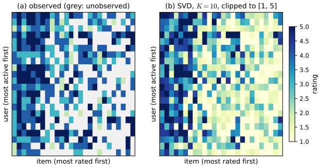
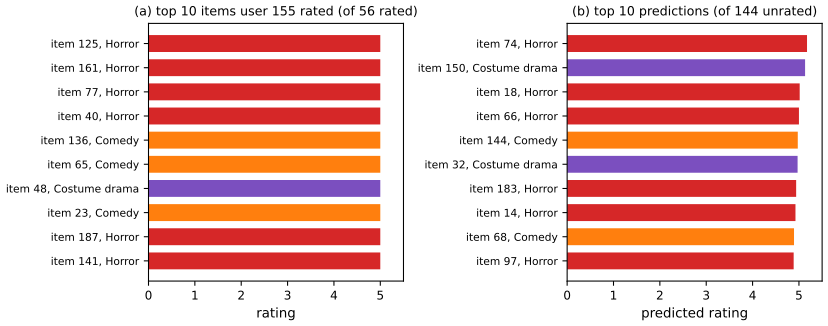
p. 745 For MovieLens-1M the book uses \(K=50\) and, "for simplicity", fits by the SVD of the dense matrix in which the missing entries are set to 0, then truncates predictions to \([1,5]\). Figure 22.3 repeats this on the simulated matrix (\(K=10\)), and Figure 22.4 lists, for one user, the items they rated highest and the highest predictions among the items they have not rated; the predicted items have the genres the user already likes, although genre is never used in training. But the "simple approximation" is not harmless: gap 22.7 shows that the zero-filled SVD shrinks every prediction by roughly the observed fraction, and compares it with the rescaled version and with proper matrix factorisation.
Filling the gap 22.7: the SVD of the zero-filled matrix is biased towards zero, and towards popular items p. 745
Derivation
Shrinkage. Let \(\bm Y^0\) be \(\bm Y\) with the unobserved entries set to 0, \(Y^0_{ui}=O_{ui}Y_{ui}\), and suppose each entry is observed independently with the same probability \(p\). Then \(\E[Y^0_{ui}]=pY_{ui}\): \(\bm Y^0\) is a noisy version of the matrix \(p\bm Y\), not of \(\bm Y\). Its truncated SVD estimates the rank-\(K\) approximation of \(p\bm Y\), so predictions are shrunk by about \(p\): for MovieLens-1M, \(p=4.47\%\); on the simulated matrix with \(K=10\) the mean prediction at unobserved entries is 0.30, against a mean rating of 3.5, and 95 percent of the predictions are below 1 (Figure 22.3b). Clipping to \([1,5]\) then hides rather than repairs the shrinkage. A common positive factor does not change the ranking of the items for one user, which is why top-\(N\) lists such as Figure 22.4 can still be sensible, but any error-based evaluation, and any use of the numbers as ratings, is wrong.
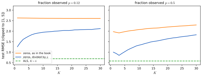
The 1/p correction. \(\bm Y^0/p\) is an unbiased estimate of \(\bm Y\) with entry variance \(Y_{ui}^2(1-p)/p\), so the truncated SVD of \(\bm Y^0/p\) is the natural rescaled estimator (universal singular value thresholding, Chatterjee, 2015). In Figure 22.S3 (training entries drawn uniformly at random so that the assumption holds) it improves greatly on the unscaled version: with \(p=0.5\) the best test RMSE falls from 1.92 to 0.85, at \(K=3\), the true latent dimension.
But it stays far worse than a proper factorisation. The noise \(\bm Y^0/p-\bm Y\) has entries of standard deviation about \(\bar y\sqrt{(1-p)/p}\), which is large when \(p\) is small, and its spectral norm is about that standard deviation times \(\sqrt M+\sqrt N\) (a heuristic from random matrix theory). Singular values of the signal below this level are lost. At \(p=0.12\) the noise level is about 283, while the first singular value (the mean rating) is about 833 and those of the latent structure only about 220: only \(K=1\) survives, and the best RMSE is 1.26. At \(p=0.5\) the noise level (about 107) is below the latent singular values, and \(K=3\) is best. Alternating least squares with baselines gets 0.69 and 0.58 on the same two problems, because it fits only the observed entries and does not turn the missing ones into noise. The book's own remark that this is "just a simple approximation to keep the demo code simple" is right as far as it goes; it should not be read as a version of the PMF fit.
Non-uniform observation. If entry \((u,i)\) is observed with probability \(P_{ui}\) (active users, popular items), then \(\E[\bm Y^0]=\bm P\circ\bm Y\) and the SVD recovers a low-rank approximation of that Hadamard product: popular items and active users are inflated relative to the rest, a built-in popularity bias. Dividing entrywise by \(P_{ui}\) (inverse propensity weighting, gap 22.1) removes it.
22.1.4 Autoencoders
pp. 745–747 Matrix factorisation is bilinear. A nonlinear alternative uses an autoencoder on the columns of the ratings matrix. Let \(\bm y_{:,i}\in\R^M\) be the ratings column of item \(i\), unknown entries set to 0. The (item-based) AutoRec model of Sedhain et al. (2015) predicts it by \[ f(\bm y_{:,i};\bm\theta)=\bm W^\T\varphi(\bm V\bm y_{:,i}+\bm\mu)+\bm b , \tag{22.11} \] with \(\bm V\in\R^{K\times M}\) mapping the ratings to a \(K\)-dimensional embedding, \(\bm W\in\R^{K\times M}\) mapping it back, \(\bm\mu\in\R^K\) the hidden biases, \(\bm b\in\R^M\) the output biases, and \(\varphi\) a nonlinearity. It is fitted by minimising the squared error on the observed entries only, plus an \(\ell_2\) penalty, \[ L(\bm\theta)=\sum_{i=1}^N\sum_{u:y_{ui}\neq?}\big(y_{ui}-f(\bm y_{:,i};\bm\theta)_u\big)^2+\frac\lambda2\big(\|\bm W\|_F^2+\|\bm V\|_F^2\big). \tag{22.12} \] A user-based version autoencodes the rows instead. The authors report that it beats restricted Boltzmann machines and local low-rank matrix approximation despite its simplicity.
Filling the gap 22.8: parameter counts, what the encoder computes, and item-based versus user-based pp. 745–746, (22.11)–(22.12)
Derivation
Counting. The item-based model has \(\bm V\) (\(KM\)), \(\bm W\) (\(KM\)), \(\bm\mu\) (\(K\)) and \(\bm b\) (\(M\)) parameters: \(2MK+M+K\), as the book says. The user-based model has input dimension \(N\) and \(2NK+N+K\). For MovieLens-1M with \(K=500\) (the size used in the AutoRec paper) that is 6,046,540 against 3,710,206 parameters. (The book's "\(\bm V\in\R^{KM}\)" is a \(K\times M\) matrix.) For comparison, a biased matrix factorisation with \(K=50\) on the same data has \((M+N)(K+1)=497{,}046\) parameters plus \(\mu\), about half a parameter per observed rating.
What the zeros do. The encoder input \(\bm V\bm y_{:,i}=\sum_{u}y_{ui}\bm V_{:,u}\) is a sum over the users who rated item \(i\) of the rating times a learned user embedding (the missing entries, being 0, contribute nothing). So the model builds the item's representation from its raters, the amortised counterpart of fitting an item vector \(\bm v_i\) by alternating least squares. The zero filling is only a convention for the input; the loss (22.12) ignores unobserved targets, so, unlike the zero-filled SVD of gap 22.7, the model is not trained to predict 0 at unobserved entries. (At prediction time the item's own known ratings are the input, and the output at the missing entries is the prediction.)
Item-based or user-based. An item-based AutoRec has one training example per item, and each example (an item's ratings column) has on average 270 observed entries in MovieLens-1M, against 166 for a user's row: the inputs are denser, the encoder is trained from more informative examples, and the authors find the item-based version better, as the book notes.
22.2 Implicit feedback
p. 747 Explicit ratings are scarce. Much more is available as implicit feedback: which items users watched, bought or clicked. One option treats the items a user selected as positives and all others as negatives, giving a positive-only matrix. Another reads the choice as a comparison: watching \(i\) but not \(j\) says that \(u\) prefers \(i\) to \(j\). The data are then tuples \((u,i,j)\) with \((u,i)\) a positive pair and \((u,j)\) a negative or unlabelled pair.
22.2.1 Bayesian personalized ranking
p. 747 To fit a score \(f(u,i;\bm\theta)\) to such tuples one needs a ranking loss that favours \(f(u,i)>f(u,j)\). A Bernoulli model for the preference, \[ p\big(y_n=(u,i,j)\mid\bm\theta\big)=\sigma\big(f(u,i;\bm\theta)-f(u,j;\bm\theta)\big), \tag{22.13} \] combined with a Gaussian prior on \(\bm\theta\) gives the MAP problem (maximise) \[ L(\bm\theta)=\sum_{(u,i,j)\in\mathcal D}\log\sigma\big(f(u,i;\bm\theta)-f(u,j;\bm\theta)\big)-\lambda\|\bm\theta\|^2 , \tag{22.14} \] where \(\mathcal D=\{(u,i,j):i\in I_u^+,\ j\in I\setminus I_u^+\}\), \(I_u^+\) the items user \(u\) selected. This is Bayesian personalised ranking (BPR; Rendle et al., 2009). In the book's example there are four items and user \(u\) chose \(I_u^+=\{i_2,i_3\}\); the implied item-by-item preference matrix, where \(+\) in row \(i\), column \(i'\) means \(u\) prefers \(i'\) to \(i\), is \[ \bm Y_u=\begin{pmatrix}\cdot&+&+&?\\-&\cdot&?&-\\-&?&\cdot&-\\?&+&+&\cdot\end{pmatrix} . \tag{22.15} \] (Nothing can be said about \(i_2\) against \(i_3\), or \(i_1\) against \(i_4\): both selected, or neither. We confirmed (22.15) by generating the matrix from the rule.) With many items the number of negatives is huge, so the loss is approximated by sampling negatives. An alternative to the log-loss is the hinge loss of SVMs (Section 17.3), \[ L\big(y_n=(u,i,j),f\big)=\max\big(m-f(u,i)+f(u,j),\,0\big), \tag{22.16} \] with margin \(m\ge0\): negatives must not score within \(m\) of the positives.
Filling the gap 22.9: the BPR likelihood, the gradient, sampling, and BPR as a surrogate for the AUC p. 747, (22.13)–(22.16)
Derivation
Likelihood and MAP. (22.13) is the Bradley-Terry-Luce model of paired comparisons: the probability that \(i\) beats \(j\) is the logistic function of the score difference \(x_{uij}=f(u,i)-f(u,j)\). Taking the tuples as independent given \(\bm\theta\) and \(\bm\theta\sim\N(\bm0,\tau^2\bm I)\), the log posterior is \(\sum_{\mathcal D}\log\sigma(x_{uij})-\frac1{2\tau^2}\|\bm\theta\|^2+\const\), which is (22.14) with \(\lambda=1/(2\tau^2)\). It is a log-posterior to be maximised, not a loss to be minimised, as the book's \(L\) might suggest.
Gradient. Since \(\frac{\d}{\d a}\log\sigma(a)=1-\sigma(a)=\sigma(-a)\), the gradient of one term is \(\sigma(-x_{uij})\,\nabla_{\bm\theta}x_{uij}\). For \(f(u,i)=b_i+\bm p_u^\T\bm q_i\) (a factorisation with item offsets) and \(g=\sigma(-x_{uij})\), stochastic gradient ascent on one sampled triple gives \[ \bm p_u\mathrel{+}=\eta\big(g(\bm q_i-\bm q_j)-\lambda\bm p_u\big),\quad \bm q_i\mathrel{+}=\eta(g\bm p_u-\lambda\bm q_i),\quad \bm q_j\mathrel{+}=\eta(-g\bm p_u-\lambda\bm q_j),\quad b_i\mathrel{+}=\eta(g-\lambda b_i),\quad b_j\mathrel{-}=\eta(g+\lambda b_j) \] (with the old \(\bm p_u\) in the item updates). The weight \(g\) is close to 1 when the triple is misordered (\(x\ll0\)) and close to 0 once it is well ordered: the algorithm concentrates on the pairs it gets wrong. The hinge loss (22.16) has \(g=\mathbb I[x<m]\): all violating triples count equally, satisfied ones not at all.
Sampling. The full sum over \(\mathcal D\) has \(\sum_un_u(N-n_u)\) terms. Drawing a positive pair \((u,i)\) uniformly from the training pairs and then \(j\) uniformly from the items outside \(I_u^+\) gives each triple the probability \(1/(|\Obs|(N-n_u))\), so the expected stochastic gradient is the gradient of \(\frac1{|\Obs|}\sum_u\frac1{N-n_u}\sum_{(i,j)}\ell_{uij}\): the objective (22.14) with the triples of user \(u\) weighted by \(1/(N-n_u)\), a mild difference from uniform weights that keeps each user's total weight proportional to \(n_u\) (this is the sampling the code uses). Uniform sampling of negatives is the simplest choice; sampling hard negatives (highly scored non-selected items) speeds up learning.
Link with the AUC. For user \(u\) the area under the ROC curve of the score ranking is \(\AUC_u=\frac1{|I_u^+||I_u^-|}\sum_{i\in I_u^+,\,j\in I_u^-}\big(\mathbb I[x_{uij}>0]+\frac12\mathbb I[x_{uij}=0]\big)\), \(I_u^-=I\setminus I_u^+\): the fraction of correctly ordered (positive, negative) pairs. The BPR terms are a smooth surrogate of the misordering count: for every real \(x\), \(\log_2(1+e^{-x})\ge\mathbb I[x\le0]\) (both sides: the left side is \(\ge1\) for \(x\le0\) and \(\ge0\) otherwise), and \(\max(0,1-x)\ge\mathbb I[x\le0]\). Hence \[ \sum_{\mathcal D_u}\log_2\big(1+e^{-x_{uij}}\big)\ \ge\ |I_u^+||I_u^-|\,(1-\AUC_u)\quad\text{(no ties)}, \] and minimising the BPR loss pushes the AUC up. (With the natural logarithm the bound needs the factor \(1/\ln2\): \(\log(1+e^{0})=\ln2<1\), so \(\log(1+e^{-x})\) alone is not an upper bound of the 0-1 loss.)
On the simulated implicit data (150 users, 100 items, 10 to 25 selections each, the last one held out; Figure 22.S5) the popularity ranking has AUC 0.726 and hit rate at 10 of 0.393; BPR with \(K=4\) after 15 epochs reaches 0.809 and 0.540, the hinge version 0.853 and 0.660, and \(K=1\) only 0.747 and 0.433 (one factor plus item offsets can hardly do better than popularity). These numbers are exactly those of the demonstration.
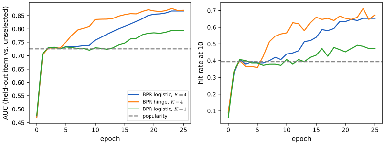
Demonstration. Bayesian personalised ranking from implicit feedback: train the model epoch by epoch, compare with popularity, and look at the ranking of one user's items. Presets: 1 BPR with \(K=4\); 2 untrained; 3 one factor; 4 \(K=8\), 40 epochs; 5 hinge loss.
See also. Section 10.2.4, SGD for logistic regression and the optimisers demonstration of this course: the BPR update is logistic-regression SGD on the feature difference \(\bm q_i-\bm q_j\) with the label always 1.
22.2.2 Factorization machines
p. 748 AutoRec treats users and items asymmetrically. A more symmetric discriminative model predicts the output (a rating, a click) for any input \(\bm x\in\R^D\); for a user-item pair, \(\bm x=[\text{one-hot}(u),\text{one-hot}(i)]\) and \(D=M+N\). The factorisation machine (FM; Rendle, 2010) is \[ f(\bm x)=\mu+\sum_{i=1}^Dw_ix_i+\sum_{i=1}^D\sum_{j=i+1}^D(\bm v_i^\T\bm v_j)x_ix_j , \tag{22.17} \] with offset \(\mu\), weights \(\bm w\in\R^D\) and a factor matrix \(\bm V\in\R^{D\times K}\) whose rows \(\bm v_i\) give each feature a \(K\)-dimensional embedding; the term \((\bm v_i^\T\bm v_j)x_ix_j\) is the interaction of features \(i\) and \(j\) with a rank-\(K\) coefficient matrix. With one-hot user and item the FM is exactly the biased factorisation (22.4), and it accepts any other features in \(\bm x\) (Section 22.3). Evaluating (22.17) directly takes \(O(KD^2)\); the book's identity (22.18)–(22.20) brings it to \(O(KD)\), and to \(O(K)\) for a one-hot user and item, but its last two lines carry a sign error (gap 22.10). The loss can be anything: squared error for explicit ratings, a ranking loss for implicit feedback. Deep factorisation machines (Guo et al., 2017) add an MLP on the concatenated embeddings, \[ f(\bm x;\bm\theta)=\sigma\big(\mathrm{FM}(\bm x)+\mathrm{MLP}(\bm x)\big), \tag{22.21} \] closely related to the wide-and-deep model (Cheng et al., 2016): the bilinear FM part memorises specific user-item interactions, the MLP part generalises through interactions of user features with item features.
Filling the gap 22.10: the factorisation machine identity (corrected sign), gradients, and FM contains matrix factorisation p. 748, (22.17)–(22.20)
Derivation
The identity. Put \(\bm a_i=x_i\bm v_i\in\R^K\). Then \(\big\|\sum_i\bm a_i\big\|^2=\sum_i\|\bm a_i\|^2+2\sum_{i<j}\bm a_i^\T\bm a_j\), so \[ \sum_{i=1}^D\sum_{j=i+1}^D(\bm v_i^\T\bm v_j)x_ix_j=\frac12\Big(\Big\|\sum_i x_i\bm v_i\Big\|^2-\sum_ix_i^2\|\bm v_i\|^2\Big)=+\frac12\sum_{k=1}^K\Big(\Big(\sum_{i=1}^Dv_{ik}x_i\Big)^2-\sum_{i=1}^Dv_{ik}^2x_i^2\Big). \] This is (22.18) (the full double sum minus its diagonal, halved) followed by exchange of the sums over \(i,j\) and \(k\); the right-hand side has a plus sign in front of \(\frac12\). The printed (22.19) and (22.20) have \(-\frac12\) in front of the bracket, which would make the pairwise sum the negative of its true value (checked numerically: for random \(\bm V\) and \(\bm x\) the pair sum is \(-78.6\) and the printed expression gives \(+78.6\)). The cost is \(O(K\,\mathrm{nnz}(\bm x))\): one pass to form \(s_k=\sum_iv_{ik}x_i\) and the sum of squares. For a one-hot user and item (two nonzeros), \(O(K)\).
It equals matrix factorisation. With active features \(u\) (the user's one-hot) and \(M+i\) (the item's), \(x_u=x_{M+i}=1\) and all other \(x_j=0\), (22.17) is \(f=\mu+w_u+w_{M+i}+\bm v_u^\T\bm v_{M+i}\), which is (22.4) with \(b_u=w_u\), \(c_i=w_{M+i}\) and the user and item vectors \(\bm v_u,\bm v_{M+i}\).
Gradients. \(\partial f/\partial\mu=1\), \(\partial f/\partial w_i=x_i\), and from the identity, \(\partial f/\partial v_{ik}=x_i\big(\sum_jv_{jk}x_j-v_{ik}x_i\big)\): the gradient of one factor needs only the shared sums \(s_k\), so one SGD step with squared error \(e=y-f\) is \(w_i\mathrel{+}=\eta(ex_i-\lambda w_i)\), \(v_{ik}\mathrel{+}=\eta(e\,x_i(s_k-v_{ik}x_i)-\lambda v_{ik})\) for the nonzero \(i\), again in \(O(K\mathrm{nnz})\) per example (this is the update the code uses, verified against finite differences).
Rank-\(K\) interaction. Writing the interaction matrix as \(\bm W=\bm V\bm V^\T\) (off-diagonal part), an FM models all \(\binom D2\) pairwise interaction coefficients with \(DK\) parameters; features that have never co-occurred in training still get an interaction through their shared factors, which is what lets an FM estimate interactions in sparse data where a full pairwise-coefficient model could not.
22.2.3 Neural matrix factorization
p. 749 Neural matrix factorisation (He et al., 2017) combines a bilinear and a deep pathway. The generalised matrix factorisation (GMF) pathway computes the element-wise product of user and item embeddings, \[ \bm z^1_{ui}=\bm P_{u,:}\odot\bm Q_{i,:},\qquad \bm P\in\R^{M\times K},\ \bm Q\in\R^{N\times K}, \tag{22.22} \] and the DNN pathway applies an MLP to the concatenation of two other embeddings, \[ \bm z^2_{ui}=\mathrm{MLP}\big([\tilde{\bm U}_{u,:},\tilde{\bm V}_{i,:}]\big), \tag{22.23} \] and the output combines them: \[ f(u,i;\bm\theta)=\sigma\big(\bm w^\T[\bm z^1_{ui},\bm z^2_{ui}]\big) . \tag{22.24} \] In the original paper the model is trained on implicit feedback with \(y_{ui}=1\) for observed interactions and 0 for sampled unobserved ones (the log loss of a Bernoulli model); it could equally be trained with the BPR loss. Figure 22.5 of the book is a network diagram and is not reproduced.
Filling the gap 22.11: GMF contains matrix factorisation; why the two pathways use separate embeddings p. 749, (22.22)–(22.24)
Derivation
GMF alone is logistic matrix factorisation. If the DNN pathway is dropped and the output weights on \(\bm z^1\) are \(\bm w_1\), the logit is \(\bm w_1^\T(\bm P_u\odot\bm Q_i)=\sum_kw_{1k}P_{uk}Q_{ik}=\bm P_u^\T\operatorname{diag}(\bm w_1)\bm Q_i\). Rescaling \(\tilde Q_{ik}=w_{1k}Q_{ik}\) absorbs the weights, so for GMF alone the weights add no generality: with \(\bm w_1=\bm 1\) it is the inner product \(\bm P_u^\T\bm Q_i\) of (22.3), and the whole model is a logistic regression with the matrix factorisation logit: \(\Pr(y_{ui}=1)=\sigma(\bm P_u^\T\bm Q_i)\), a Bernoulli model for implicit data in place of the Gaussian of (22.10). Learned output weights matter only because the logit also contains the DNN pathway: they set how much of the logit comes from the bilinear part and how much from the MLP.
Separate embeddings. Using different embedding matrices \((\bm P,\bm Q)\) and \((\tilde{\bm U},\tilde{\bm V})\) lets the two pathways have different dimensions and different roles, and avoids forcing a single vector to serve both a product-form interaction and a concatenation-form one. A caveat from later work (Rendle et al., 2020): an MLP has difficulty learning a dot product from concatenated embeddings, and a well-tuned plain matrix factorisation often matches neural matrix factorisation, which is the reason for keeping an explicit bilinear pathway.
22.3 Leveraging side information
pp. 749–750 So far the predictor sees only the integer ids of the user and the item. This fails for a new user or item that has no history (the cold start problem): there is no vector to look up. To overcome it, use side information: for items, metadata such as title text, cover images, location or price; for users, past searches, purchases, or the friendship graph; and context such as time of day or the most recent items viewed. In a factorisation machine this is a matter of widening \(\bm x\) beyond the two one-hot blocks (Figure 22.6 of the book shows such a design matrix: user id, movie id, other movies the user rated (normalised), time, last movie rated, target), and the same input can be fed to deep FMs or neural matrix factorisation. The Caser model (Tang and Wang, 2018) embeds the last few items viewed and treats the resulting \(M\times K\) array as an image for a convolutional layer.
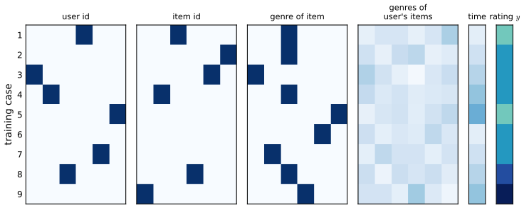
Filling the gap 22.12: how an FM with item attributes predicts for an unseen item, and what it cannot fix pp. 749–750
Derivation
Prediction for a new item. Give each item a one-hot id feature (index \(M+i\)) and each genre a feature (index \(M+N+g\)); an input is then three active features \(\{u,\,M+i,\,M+N+g(i)\}\). By (22.17) with all \(x=1\), \[ f=\mu+w_u+w_{M+i}+w_{g}+\bm v_u^\T\bm v_{M+i}+\bm v_u^\T\bm v_g+\bm v_{M+i}^\T\bm v_g . \] A new item has never appeared in training, so with \(\ell_2\) regularisation its id parameters \(w_{M+i}\) and \(\bm v_{M+i}\) sit at their prior mean 0, and the prediction is \(\mu+w_u+w_g+\bm v_u^\T\bm v_g\): the user's offset plus the genre's offset plus the user's affinity to the genre, all learned from the other items of the genre. An id-only model has nothing but \(\mu+b_u\). Seen the other way, the item vector is \(\bm v_{M+i}+\bm v_g\): the attributes provide the prior mean of the item vector, and the id-specific part is a correction learned as data arrive (a hierarchical, partially pooled model).
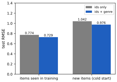
Numbers. On the simulated data we hold out 40 of the 200 items entirely (all of their ratings are test data: 1,450 test ratings) and train on the rest. Test RMSE on warm items (ratings of items seen in training) is 0.774 for the id-only FM and 0.729 with the genre; on cold items it is 1.042 and 0.976 (Figure 22.S6). The gain is 0.07 rating points: genre says a lot about the latent direction of an item (the simulated item vectors are genre centres plus noise) but nothing about its individual popularity offset \(c_i\) or its within-genre deviation, and these remain unknown until ratings arrive. Richer side information (text, images) can in principle reveal more.
The same mechanism for users (a new user's age group, location, or last items viewed) and for context (time), as in Figure 22.6.
22.4 Exploration-exploitation tradeoff
pp. 750–751 Recommendation has a feature that ordinary prediction does not: the training data are a consequence of what earlier versions of the system recommended. A system that shows a slate of videos and learns from the clicks gets feedback only on what it showed; some other video might have pleased the user even more, but that counterfactual is unobservable unless the system takes a chance on items whose response is uncertain. This is the exploration-exploitation trade-off, and the feedback loop (Bottou et al., 2013) can lock a system into a mediocre policy. A change of policy may also pay off only after a long time, which is why one often formulates the problem as reinforcement learning (the book refers to its sequel for that). Here we study the simplest case, the click bandit, and a second tool for the same loop: evaluating a new policy from data collected by an old one.
The model: \(K\) items (arms); showing item \(a\) yields a click with probability \(\mu_a\), unknown. With \(\mu^*=\max_a\mu_a\) and gaps \(\Delta_a=\mu^*-\mu_a\), the regret after \(T\) rounds is \(\mathrm{Reg}_T=\sum_{t=1}^T(\mu^*-\mu_{a_t})\), the click probability lost against always showing the best item. We compare four policies: greedy (show the item with the best observed click rate after showing each once), ε-greedy (with probability \(\epsilon\) show a uniformly random item), UCB1 (show \(\arg\max_a\hat\mu_a+\sqrt{2\ln t/n_a}\), an optimistic estimate), and Thompson sampling (draw \(\theta_a\sim\mathrm{Beta}(1+s_a,1+n_a-s_a)\), the posterior of a Beta(1,1) prior, and show the item with the largest draw).
Filling the gap 22.13: the regret decomposition, why greedy and fixed-ε policies have linear regret, and the UCB1 and Thompson guarantees pp. 750–751
Derivation
Decomposition. Let \(N_a(T)\) be the number of times item \(a\) is shown. Then \(\mathrm{Reg}_T=\sum_a\Delta_aN_a(T)\) (group the rounds by the item shown), so the expected regret is \(\sum_a\Delta_a\E[N_a(T)]\): a policy has small regret iff it shows each suboptimal item rarely. (Confirmed numerically on simulated runs.)
Fixed \(\epsilon\) gives linear regret. In every round, with probability \(\epsilon\) the item is chosen uniformly at random independently of the past, so the expected regret of that round is at least \(\epsilon\bar\Delta\), \(\bar\Delta=\frac1K\sum_a\Delta_a\); every round's regret is nonnegative, so \(\E[\mathrm{Reg}_T]\ge\epsilon\bar\Delta T\). With the six items of Figure 22.S7 (\(\bar\Delta=0.147\), \(\epsilon=0.1\)) the bound is 0.0147 per round and the simulation shows a slope of 0.018. Decaying \(\epsilon_t\propto K/(\Delta^2t)\) restores logarithmic regret (Auer et al., 2002) but needs knowledge of the smallest gap.
Greedy can lock in. Take two items with \(\mu_1>\mu_2\) and a greedy policy that shows each once and then the one with the higher empirical rate. With probability \((1-\mu_1)\mu_2>0\) the first show of item 1 gives no click and the first show of item 2 gives a click. Then the empirical rates are 0 and 1, item 2 is shown, and as long as item 2 has at least one click (it already has one) its empirical rate \(s/n\ge1/n\) stays strictly above item 1's frozen rate 0: item 1 is never shown again. The regret then grows as \(\Delta T\), so \(\E[\mathrm{Reg}_T]\ge(1-\mu_1)\mu_2(\mu_1-\mu_2)(T-2)\): linear regret, for any gap, however small the probability of the unlucky start. This is the feedback loop of the book in its barest form: an item that is not shown cannot be corrected. In the six-item example the best item is shown fewer than half the time in 60 percent of runs (Figure 22.S7), and in the two-item example with \(\mu=(0.5,0.45)\) a simulation of 4,000 runs gives expected regret 6.1 at \(T=400\) against the lower bound 4.5.
UCB1. The index \(U_a(t)=\hat\mu_a+\sqrt{2\ln t/n_a}\) adds a bonus that shrinks as an item is shown and grows slowly with \(t\) for items left alone. By Hoeffding's inequality, \(\Pr(\hat\mu_{a,n}\ge\mu_a+\sqrt{2\ln t/n})\le e^{-2n\cdot2\ln t/n}=t^{-4}\), and the same for the lower tail. A suboptimal item \(a\) can be shown at time \(t\) only if (i) the index of the best item is below \(\mu^*\), (ii) the empirical rate of \(a\) exceeds its mean by more than its bonus, or (iii) \(\Delta_a\le2\sqrt{2\ln t/n_a}\), i.e. \(n_a\le8\ln t/\Delta_a^2\). Events (i) and (ii) have probability \(\le t^{-4}\) per candidate pull count, and summing the union bound over \(t\) and the pull counts gives a constant \(1+\pi^2/3\); hence (Auer, Cesa-Bianchi and Fischer, 2002) \[ \E[N_a(T)]\le\frac{8\ln T}{\Delta_a^2}+1+\frac{\pi^2}3,\qquad \E[\mathrm{Reg}_T]\le\sum_{a:\Delta_a>0}\Big(\frac{8\ln T}{\Delta_a}+\Big(1+\frac{\pi^2}3\Big)\Delta_a\Big). \] The bound is logarithmic in \(T\) but conservative: for the six items and \(T=3000\) it is 2,004, while the simulated regret is 193. The matching lower bound is Lai and Robbins (1985): any policy that is consistent (sub-polynomial regret on every problem) has \(\liminf\E[N_a(T)]/\ln T\ge1/\KL(\mu_a\|\mu^*)\), so logarithmic growth cannot be improved in order. UCB1's constant is not optimal, and with many rounds of near-ties it explores a lot (at \(T=1000\) with six items its regret, 94, is higher than that of a well-chosen \(\epsilon\)-greedy).
Thompson sampling. With a Beta(1,1) prior and Bernoulli clicks the posterior of \(\mu_a\) after \(s_a\) clicks in \(n_a\) shows is Beta\((1+s_a,1+n_a-s_a)\) (conjugacy, Section 4.6.2), and showing the item with the largest posterior draw shows each item with the posterior probability that it is the best: exploration is spent in proportion to the remaining uncertainty and stops by itself as the posteriors concentrate. It has logarithmic regret matching the Lai-Robbins constant for Bernoulli arms (Agrawal and Goyal, 2012; Kaufmann, Korda and Munos, 2012). In Figure 22.S7 (60 runs, \(T=3000\)) the average regrets are 392 (greedy), 83 (\(\epsilon\)-greedy, \(\epsilon=0.1\)), 193 (UCB1) and 51 (Thompson sampling).
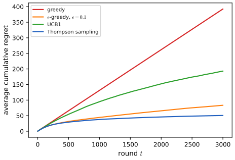
Demonstration. The exploration-exploitation trade-off in a recommender: change \(\epsilon\), the horizon, the number of runs and the items, and see the regret and where the exposure goes. Presets: 1 six items; 2 pure greedy; 3 too much exploration; 4 two close items; 5 ten items.
See also. Section 4.6.2, the beta-binomial model (the Thompson posterior) and the conjugate updating demonstration.
Filling the gap 22.14: evaluating a new policy on logged data, inverse propensity weighting pp. 750–751
Derivation
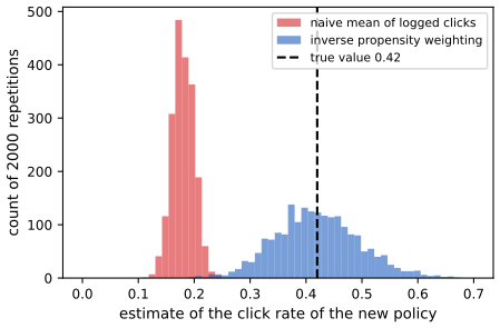
The problem. A deployed policy \(e\) (the logging policy) showed item \(a_n\) with known probability \(e(a_n)\) and observed a click \(r_n\in\{0,1\}\), \(n=1,\dots,n\). We want the click rate \(V(\pi)=\sum_a\pi_a\mu_a\) that a different policy \(\pi\) would have achieved, without deploying it. The average of the logged clicks is not that: its expectation is \(\sum_ae_a\mu_a=V(e)\), the value of the old policy. Because the logging policy chose what to show, the logged data over-represent items it favoured: the feedback loop again.
Inverse propensity weighting. Re-weight each logged click by how much more (or less) often \(\pi\) would have shown that item: \[ \hat V_{\mathrm{IPS}}(\pi)=\frac1n\sum_{n}r_n\,\frac{\pi(a_n)}{e(a_n)} . \] If \(e_a>0\) whenever \(\pi_a>0\) (positivity), then \(\E\big[r\,\pi(a)/e(a)\big]=\sum_ae_a\mu_a\pi_a/e_a=\sum_a\pi_a\mu_a=V(\pi)\): unbiased. For Bernoulli clicks \(\E[r^2]=\mu_a\), so \[ \var(\hat V_{\mathrm{IPS}})=\frac1n\Big(\sum_a\frac{\pi_a^2\mu_a}{e_a}-V(\pi)^2\Big), \] which is large when \(\pi\) favours items that the logging policy rarely showed (\(e_a\) small): exactly the regions where the logs say least. With contexts \(\bm x\) the weight is \(\pi(a\mid\bm x)/e(a\mid\bm x)\). Capping the weights, or normalising them by their sum, trades a little bias for much lower variance. This is the same Horvitz-Thompson idea as in gap 22.1, now with the logged action in the role of the observation indicator, and it is the basis of off-policy evaluation and of learning from logged bandit feedback (Bottou et al., 2013; Schnabel et al., 2016).
Example. Three items with click probabilities \((0.1,0.3,0.5)\), logging policy \(e=(0.7,0.2,0.1)\), new policy \(\pi=(0.1,0.2,0.7)\): \(V(e)=0.18\), \(V(\pi)=0.42\). With \(n=400\) logged rounds repeated 2,000 times (Figure 22.S8) the naive average is centred at 0.18 (the old policy's value), while the inverse-propensity estimate is centred at 0.419, with standard deviation 0.077 (the formula gives \(\sqrt{0.00584}=0.076\)).
Exercises
Chapter 22 of the book has no end-of-chapter exercises. Instead, here are three practice problems of my own, each with a complete solution (hidden); they use the results above.
Problem 22.1 (parameter counts and the ratio to the data). For MovieLens-1M (\(M=6040\), \(N=3706\), \(1{,}000{,}209\) ratings) compare the number of parameters of the biased factorisation (22.4) with \(K=50\), of item-based AutoRec (22.11) with a hidden layer of \(K=500\) units, and a deep FM with embedding size 16 on one-hot user and item (ignore the MLP). Which has the most parameters per observed rating?
Solution
Biased factorisation: \(\mu\), \(M+N=9746\) offsets and \((M+N)K=487{,}300\) factors: 497,047 parameters, 0.50 per rating. Item-based AutoRec: \(2MK+M+K=6{,}040{,}000+6{,}040+500=6{,}046{,}540\), 6.05 per rating (the user-based version has \(2\cdot3706\cdot500+3706+500=3{,}710{,}206\)). FM (22.17) with \(D=M+N=9746\) features and \(K=16\): \(1+D+DK=1+9746+155{,}936=165{,}683\), 0.17 per rating. AutoRec is by far the most over-parameterised relative to the data, which is why it relies on the penalty (22.12).
Problem 22.2 (an FM by hand). Let \(D=4\), \(K=2\), \(\mu=3\), \(\bm w=(0.5,-0.2,0.1,0.3)\), \(\bm v_1=(1,0)\), \(\bm v_2=(0,1)\), \(\bm v_3=(1,1)\), \(\bm v_4=(-1,2)\), and \(\bm x=(1,0,1,2)\). Compute \(f(\bm x)\) both from (22.17) and from the linear-time form, and state the value of the linear-time form with the book's printed sign.
Solution
Linear part: \(\mu+w_1+w_3+2w_4=3+0.5+0.1+0.6=4.2\). Pairs among the nonzero features \(\{1,3,4\}\): \(\bm v_1^\T\bm v_3x_1x_3=1\cdot1\cdot1=1\); \(\bm v_1^\T\bm v_4x_1x_4=(-1)(2)=-2\); \(\bm v_3^\T\bm v_4x_3x_4=(-1+2)(2)=2\). Sum \(=1\), so \(f=5.2\). Linear-time form: \(s_k=\sum_iv_{ik}x_i\): \(s_1=1\cdot1+1\cdot1+(-1)\cdot2=0\), \(s_2=0+1+4=5\); \(\sum_iv_{ik}^2x_i^2\): for \(k=1\): \(1+1+4=6\); \(k=2\): \(0+1+16=17\). So \(\frac12[(0-6)+(25-17)]=\frac12(-6+8)=1\): matches. With the printed leading minus the value would be \(-1\), and \(f\) would be 3.2, wrong.
Problem 22.3 (inverse propensity weighting). Two items, click probabilities \(\mu=(0.2,0.6)\). The logging policy shows item 1 with probability 0.9. The new policy always shows item 2. (a) What do the naive and the inverse-propensity estimates converge to? (b) Give the variance of the latter for \(n\) logged rounds.
Solution
(a) The naive estimate converges to \(V(e)=0.9\cdot0.2+0.1\cdot0.6=0.24\); the true value of the new policy is \(V(\pi)=0.6\), and the inverse-propensity estimate \(\frac1n\sum r_n\mathbb I[a_n=2]/0.1\) is unbiased for it: \(\E=0.1\cdot0.6/0.1=0.6\). (b) \(\var=\frac1n\big(\pi_2^2\mu_2/e_2-V(\pi)^2\big)=\frac1n(0.6/0.1-0.36)=5.64/n\): only the 10 percent of logged rounds in which item 2 was shown carry information, each weighted by 10, so one needs \(n\approx5.64/0.0025=2{,}256\) rounds for a standard error of 0.05.
Demonstrations
| Page | What it shows | In the notes |
|---|---|---|
| Matrix factorisation by alternating least squares | Biased factorisation of the simulated ratings by alternating ridge regressions: the number of factors, the penalty, the number of iterations, baselines on or off; training and test RMSE, the true-mean floor, and the item vectors on their principal axes. Presets: 1 baselines only; 2 one factor; 3 \(K=4\); 4 overfitting; 5 too much penalty; 6 no baselines. | 22.1.3, gap 22.3, gap 22.4, gap 22.6 |
| Bayesian personalised ranking | SGD on sampled (user, positive, negative) triples with the logistic or hinge loss; AUC and hit rate at 10 against the epoch, with the popularity ranking as baseline, and the ranking of one user's items. Presets: 1 \(K=4\); 2 untrained; 3 one factor; 4 \(K=8\), 40 epochs; 5 hinge loss. | 22.2.1, gap 22.9 |
| The exploration-exploitation trade-off | Greedy, ε-greedy, UCB1 and Thompson sampling in a click bandit: average regret over many runs with common random numbers, the share of runs in which the best item is starved, and the exposure of each item. Presets: 1 six items; 2 pure greedy; 3 too much exploration; 4 two close items; 5 ten items, 100 runs. | 22.4, gap 22.13 |
Notes on the book
Corrections and clarifications (Chapter 22)
- (22.1), collaborative filtering. The sum of similarity-weighted ratings is not normalised, so it is not a weighted average: with \(n\) identical neighbours the prediction scales with \(n\). Divide by \(\sum|\operatorname{sim}|\) and centre the ratings (gap 22.2). In the text the "sets" \(S_u=\{Y_{u,i}\neq?:i\in I\}\) should be the sets of items the user rated, \(\{i:Y_{u,i}\neq?\}\).
- (22.2). The sum over observed entries is the masked norm \(\|P_\Obs(\bm Z-\bm Y)\|_F^2\), not \(\|\bm Z-\bm Y\|_F^2\) (equal only when nothing is missing) (gap 22.3).
- Section 22.1.3, convexity. The factorisation objective is non-convex in \((\bm U,\bm V)\) even when every entry is observed (the pairs \((\bm U,\bm V)\) and \((-\bm U,-\bm V)\) have equal value while their midpoint is worse); what missing entries add is spurious local minima (gap 22.3).
- (22.5)–(22.9). With the penalty inside the sum over observed pairs, parameter \(b_u\) is penalised \(n_u\) times, and this is the objective that SGD optimises; the usual ridge form (each parameter once) is a rescaling of \(\lambda\) per user and item (gap 22.4, gap 22.5). The updates (22.6)–(22.9) absorb a factor 2 into \(\eta\); \(\eta>0\) is needed for a descent step.
- Section 22.1.3.1, (22.10). "The NLL of this model is equivalent to the matrix factorisation objective in Equation (22.2)": equivalent for the minimiser, not including the regulariser, which comes from the prior (MAP with \(\lambda=\sigma^2/\tau^2\), gap 22.6).
- Section 22.1.3.2. The plotted movie vectors are called \(\bm u_i\); the item vectors are \(\bm v_i\) in the notation of (22.3)–(22.9).
- Section 22.1.3.3, zero-filled SVD. Setting missing ratings to 0 does not give a version of PMF: it estimates the matrix \(p\bm Y\), so predictions are shrunk by about the observed fraction (4.5 percent for MovieLens-1M) and are biased towards popular items; truncating to \([1,5]\) hides this. The numbers are rankings at best, not ratings (gap 22.7).
- (22.11)–(22.12). \(\bm V\) and \(\bm W\) are \(K\times M\) matrices (the text writes \(\mathbb R^{KM}\)); the parameter count \(2MK+M+K\) is right (gap 22.8).
- (22.14). It is a log posterior to be maximised, with \(\lambda=1/(2\tau^2)\) for a Gaussian prior of variance \(\tau^2\) (gap 22.9). With the natural logarithm, \(\log(1+e^{-x})\) is not an upper bound of the 0-1 loss; \(\log_2\) is.
- (22.19) and (22.20), the sign. The leading factor should be \(+\frac12\), not \(-\frac12\): with the printed sign the expression equals minus the pairwise sum (gap 22.10; checked numerically, and in Problem 22.2).
- Sections 22.1.1 and 22.1.3. The assumption that data are missing at random is convenient and often false (users rate what they like); the consequences and a correction are in gap 22.1.
References
- Murphy, K. P. (2022). Probabilistic Machine Learning: An Introduction. MIT Press, Cambridge, MA. Chapter 22, pp. 741–751. probml.github.io/pml-book/book1.html.
- Agrawal, S. and Goyal, N. (2012). Analysis of Thompson sampling for the multi-armed bandit problem. Conference on Learning Theory.
- Auer, P., Cesa-Bianchi, N. and Fischer, P. (2002). Finite-time analysis of the multiarmed bandit problem. Machine Learning, 47, 235–256.
- Bertsekas, D. P. (1999). Nonlinear Programming, 2nd edition. Athena Scientific, Belmont, MA.
- Bottou, L. (2010). Large-scale machine learning with stochastic gradient descent. Proceedings of COMPSTAT.
- Bottou, L., Peters, J., Quinonero-Candela, J., Charles, D. X., Chickering, D. M., Portugaly, E., Ray, D., Simard, P. and Snelson, E. (2013). Counterfactual reasoning and learning systems: the example of computational advertising. Journal of Machine Learning Research, 14, 3207–3260.
- Bradley, R. A. and Terry, M. E. (1952). Rank analysis of incomplete block designs: I. The method of paired comparisons. Biometrika, 39, 324–345.
- Chatterjee, S. (2015). Matrix estimation by universal singular value thresholding. Annals of Statistics, 43(1), 177–214.
- Cheng, H.-T. et al. (2016). Wide and deep learning for recommender systems. Workshop on Deep Learning for Recommender Systems.
- Guo, H., Tang, R., Ye, Y., Li, Z. and He, X. (2017). DeepFM: a factorization-machine based neural network for CTR prediction. International Joint Conference on Artificial Intelligence.
- He, X., Liao, L., Zhang, H., Nie, L., Hu, X. and Chua, T.-S. (2017). Neural collaborative filtering. International World Wide Web Conference.
- Kaufmann, E., Korda, N. and Munos, R. (2012). Thompson sampling: an asymptotically optimal finite-time analysis. Algorithmic Learning Theory.
- Koren, Y., Bell, R. and Volinsky, C. (2009). Matrix factorization techniques for recommender systems. Computer, 42(8), 30–37.
- Lai, T. L. and Robbins, H. (1985). Asymptotically efficient adaptive allocation rules. Advances in Applied Mathematics, 6, 4–22.
- Marlin, B. M., Zemel, R. S., Roweis, S. T. and Slaney, M. (2011). Recommender systems, missing data and statistical model estimation. International Joint Conference on Artificial Intelligence.
- Mazumder, R., Hastie, T. and Tibshirani, R. (2010). Spectral regularization algorithms for learning large incomplete matrices. Journal of Machine Learning Research, 11, 2287–2322.
- Rendle, S. (2010). Factorization machines. IEEE International Conference on Data Mining.
- Rendle, S., Freudenthaler, C., Gantner, Z. and Schmidt-Thieme, L. (2009). BPR: Bayesian personalized ranking from implicit feedback. Uncertainty in Artificial Intelligence.
- Rendle, S., Krichene, W., Zhang, L. and Anderson, J. (2020). Neural collaborative filtering vs. matrix factorization revisited. ACM Conference on Recommender Systems.
- Rubin, D. B. (1976). Inference and missing data. Biometrika, 63(3), 581–592.
- Salakhutdinov, R. and Mnih, A. (2008). Probabilistic matrix factorization. Advances in Neural Information Processing Systems, 20.
- Schnabel, T., Swaminathan, A., Singh, A., Chandak, N. and Joachims, T. (2016). Recommendations as treatments: debiasing learning and evaluation. International Conference on Machine Learning.
- Sedhain, S., Menon, A. K., Sanner, S. and Xie, L. (2015). AutoRec: autoencoders meet collaborative filtering. International World Wide Web Conference (Companion).
- Srebro, N. and Jaakkola, T. (2003). Weighted low-rank approximations. International Conference on Machine Learning.
- Tang, J. and Wang, K. (2018). Personalized top-N sequential recommendation via convolutional sequence embedding. ACM International Conference on Web Search and Data Mining.
All explanations, derivations, figures and code on this page are my own; the figures use simulated data and are drawn from scratch, and the results are cited to Murphy (2022) and to the original papers.