Deep generative models: from Bishop to Murphy
Bishop's latent-variable models are linear, and their likelihoods are tractable. Murphy's Advanced Topics keeps the same questions (what is the latent structure, what is the density, how do we fit it) and answers them with neural networks. Four lectures follow the same route: a continuous latent variable with an encoder and decoder, invertible maps that keep the density exact, factorisations along an ordering, and reverse-time noise. Each lecture has a demonstration.
Where this sits
It builds on Chapter 9 (mixtures and EM), Chapter 10 (variational inference), Chapter 12 (probabilistic PCA), Chapter 8 (the chain rule and directed graphs), and Chapter 13 (sequential data). Murphy's section numbers refer to the December 2025 draft; the final numbering may differ. Where a demonstration reproduces an experiment, the notebook of Murphy's book code (pyprobml, MIT licence) is named in its box.
Starting point: sequential Bayes
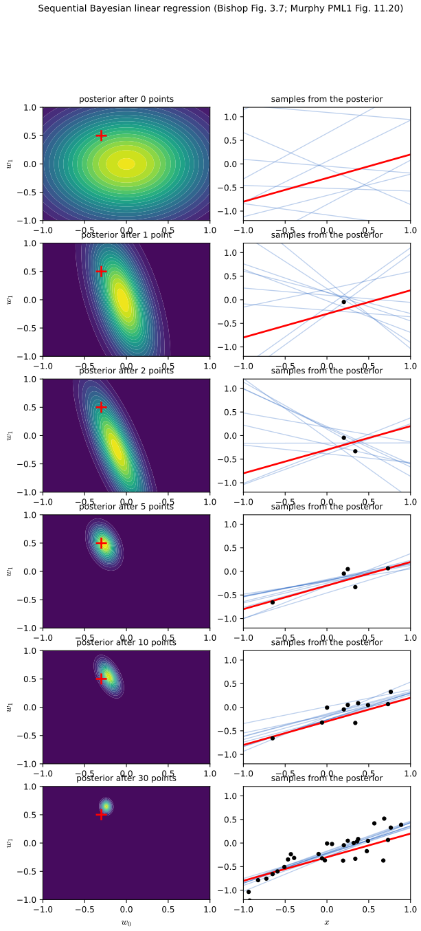
Murphy reuses one classical construction (PML1 Section 11.6.1, Figure 11.20; Bishop Section 3.3): a Gaussian posterior over the parameters of a line, updated one point at a time. Each new point adds one term to the precision, and the mean moves towards the data. The posterior after all points is the same whatever the order (Bishop (3.53)–(3.54)), and the Python update agrees with that closed form to 2e-16.
fig_sequential. Download: PDF · SVGLecture 1: variational autoencoders
From the mixture to a continuous latent variable. The Chapter 9 model has a discrete latent variable (which cluster generated a point) and closed-form EM updates. A variational autoencoder (Murphy Section 21.2) keeps a latent variable but makes it continuous, with a neural decoder pθ(x | z) and an encoder qφ(z | x) that is learned rather than computed. Training maximises the evidence lower bound
\[ \mathrm{ELBO}(\mathbf{x}) = \E_{q_\phi(\mathbf{z}\given\mathbf{x})}\big[\ln p_\theta(\mathbf{x}\given\mathbf{z})\big] - \KL\big(q_\phi(\mathbf{z}\given\mathbf{x})\,\|\,\N(\mathbf{0},\mathbf{I})\big), \]which is Bishop's (10.2) with the decoder written out. For a diagonal Gaussian encoder the KL term has a closed form, and the expectation is made differentiable by the reparameterisation z = μφ(x) + σφ(x) ⊙ ε, ε ∼ N(0, I). Two consequences matter in practice: the KL term is a penalty that pulls the codes towards the prior, and the reconstruction term, with a Gaussian likelihood of fixed variance, is a squared error.
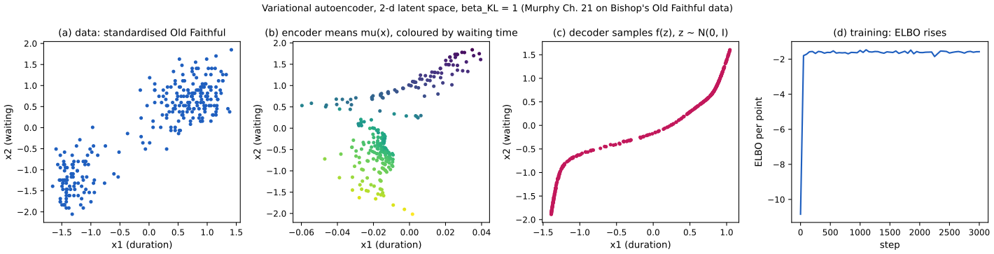
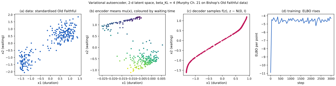
Posterior collapse. If the decoder can explain the data without the latent code, the encoder matches the prior in some directions and those latent directions carry no information (Murphy Section 21.4). The experiment below trains the VAE on the Chapter 9 data and shows exactly this.
fig_vae. Download: PDF · SVGnotebooks/book2/21/vae_latent_space.ipynb (pyprobml, MIT licence) trains a two-dimensional VAE on MNIST. The reproduction is code/bridge_vae_mnist_book.py.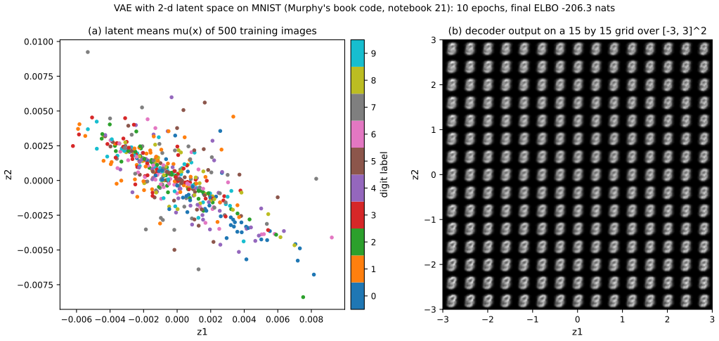
Lecture 2: normalizing flows
Exact densities through invertible maps. A VAE has no exact likelihood; its ELBO is a bound. A normalizing flow keeps the likelihood exact. Take a base density pZ (Gaussian or Student-t) and an invertible map x = f(z). The change-of-variables formula of Bishop Section 1.2.1 gives
\[ p_X(\mathbf{x}) = p_Z\big(f^{-1}(\mathbf{x})\big)\,\Big|\det \frac{\partial f^{-1}}{\partial \mathbf{x}}\Big| . \]A composition of maps multiplies the Jacobians, so the log-densities add. The design problem is to make the map flexible and the Jacobian cheap. Affine coupling layers (RealNVP, Murphy Section 23.2) split the coordinates into two halves. One half passes through unchanged and sets a scale and shift for the other: xb' = xb exp(s(xa)) + t(xa). The Jacobian is triangular, so its determinant is exp(∑ s), and the inverse is explicit. Alternating the halves between layers lets every coordinate change.
Two practical points. Bounding the scale with tanh keeps the layers stable. And a flow can only move mass continuously: it can stretch and squeeze a Gaussian into a multimodal shape (a bijection cannot fold mass onto itself), and the density it produces is exact, so a poor fit shows up as a visible misfit rather than a hidden bound.
notebooks/book2/23/flow_2d_mlp.ipynb (pyprobml, MIT licence): the target y = 0.8 x2 + 0.2 ε, x = 0.6 ε, learned by maximum likelihood. Reproduction: code/bridge_flow_book.py.
Sampling a flow is the forward map applied to base samples; evaluating a density is the inverse map plus the log-determinant. The demo shows both.
Lecture 3: autoregressive models
Factorise along an ordering. The chain rule of Bishop Chapter 8 writes any joint distribution as a product of conditionals: p(x) = ∏i p(xi | x<i). An autoregressive model fixes an ordering (raster order for pixels) and learns each conditional with a network that may only read earlier variables. The likelihood is then exact and easy to evaluate, and sampling runs one variable at a time. Murphy covers the neural forms in Section 22.2 (NADE) and Section 22.3 (causal convolutions), and attention-based models in Section 22.4.
The mask is what makes it a density. If the conditional for pixel i reads pixel i+1, the product of conditionals can fail to be a normalised joint distribution: the probabilities it assigns need not add up to 1. The demo checks this on a 2 by 2 image, summing the product of conditionals over all 16 configurations. The visible symptom is copying: the model reproduces earlier rows instead of synthesising new structure.
Note on this demonstration. The book's code has a PixelCNN notebook only in its miscellaneous folder (notebooks/misc/pixel_cnn_vq_vae.ipynb, pyprobml, MIT licence), not with its autoregressive chapter. This demonstration is therefore written for the course: a causal logistic model with a fixed weight window, not a trained network. Reproducing the PixelCNN notebook is planned.
Lecture 4: diffusion models
Reverse a noising chain. Diffusion models (Murphy Chapter 25) define a forward chain that adds Gaussian noise in small steps until the data are destroyed:
\[ \mathbf{x}_t = \sqrt{\bar\alpha_t}\,\mathbf{x}_0 + \sqrt{1-\bar\alpha_t}\,\boldsymbol\epsilon , \qquad \boldsymbol\epsilon \sim \N(\mathbf{0},\mathbf{I}), \]where αt = 1 − βt and ᾱt is their running product. Because the forward steps are Gaussian, the marginal at each time is known in closed form, which is the link to the Gaussian conditionals of Bishop Section 2.3. Generation runs the chain backwards. The denoising model of Murphy Section 25.2 predicts the noise ε in xt, and one reverse step removes a fraction of it and adds fresh noise.
Score matching. The noise prediction is equivalent to estimating the score ∇x log pt(x) (Murphy Section 25.3): εθ(xt) = −√(1 − ᾱt) ∇ log pt. For a target that is a Gaussian mixture the score of every noised marginal is available in closed form, so the demo runs the exact reverse sampler without training, which isolates the role of the noise schedule. The schedule matters: a linear schedule and a cosine schedule destroy the structure at different rates, and an abrupt early jump in the variance dissolves fine detail before the coarse structure is set.
notebooks/book2/25/diffusion_spiral_non_neural.ipynb (pyprobml, MIT licence): the swirl data, the gamma schedule gamma(t) = -8 + 13t with variance sigmoid(gamma(t)), and the forward noising. The notebook has no sampler; the reverse step in the demo is built on the exact score of the noised data. Reproduction: code/bridge_diffusion_book.py.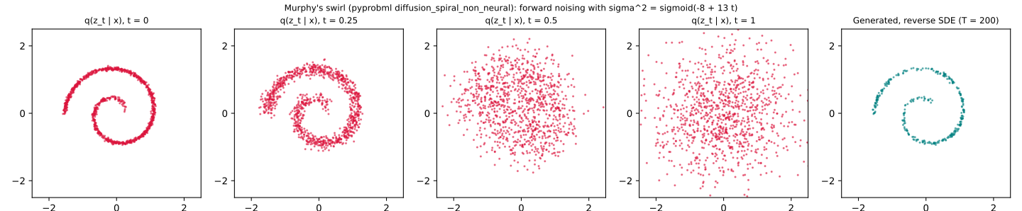
References
- Bishop, C. M. (2006). Pattern Recognition and Machine Learning. Springer, New York.
- Murphy, K. P. (2025). Probabilistic Machine Learning: Advanced Topics. Draft of 10 December 2025 (MIT Press, in preparation). Chapters 21 to 25.
- Murphy, K. P. (2025). Probabilistic Machine Learning: An Introduction. Draft of 18 April 2025 (MIT Press, in preparation). Section 11.6.1.
- Kingma, D. P. and Welling, M. (2014). Auto-encoding variational Bayes. International Conference on Learning Representations. arXiv:1312.6114.
- Dinh, L., Sohl-Dickstein, J. and Bengio, S. (2017). Density estimation using Real NVP. International Conference on Learning Representations. arXiv:1605.08803.
- Ho, J., Jain, A. and Abbeel, P. (2020). Denoising diffusion probabilistic models. Advances in Neural Information Processing Systems 33. arXiv:2006.11239.