Neural Networks
Linear models in fixed basis functions (Chapters 3 and 4) are easy to fit but cannot adapt their features to the data. A neural network keeps the form "linear combination of basis functions" but lets each basis function be a nonlinear function of a linear combination of the inputs, with adjustable coefficients. This chapter covers how such networks compute (Section 5.1), what error function to minimise and why (5.2), how to compute its gradient in time proportional to the number of weights (backpropagation, 5.3) and its second derivatives (5.4), how to control over-fitting and build in invariances (5.5), how to model multimodal targets (5.6), and how to treat the weights in a Bayesian way (5.7).
Ch. 1 Introduction Ch. 2 Probability distributions Ch. 3 Linear regression Ch. 4 Linear classification Ch. 5 Neural networks Ch. 6 Kernel methods Ch. 7 Sparse kernel machines Ch. 8 Graphical models Ch. 9 Mixture models and EM Ch. 10 Approximate inference Ch. 11 Sampling methods Ch. 12 Continuous latent variables Ch. 13 Sequential data Ch. 14 Combining models
How to read these notes
They follow the book. Sections carry Bishop's numbers (5.1, 5.3.4, ...) and every displayed equation that appears in the book carries the book's own equation number, e.g. (5.53), so you can read these notes next to the book. Equations without a number are steps that the book skips.
Filling the gaps. Wherever the book says that a result "can be verified", is "straightforward", or leaves it to an exercise, an orange Filling the gap box or a proof gives the full argument. Proofs and derivations start hidden: open one with its bar, or use the button below.
Figures and demonstrations. The numerical figures of the chapter are reproduced from scratch by the Python code; the schematic ones are redrawn. The ▶ Demo boxes open an interactive demonstration already set to the case being discussed. Standard identities (matrix calculus, the Woodbury identity, Gaussian marginals and conditionals, the softmax) are proved once in the mathematical toolkit and linked from here.
Main reference
C. M. Bishop, Pattern Recognition and Machine Learning, Springer (2006), Chapter 5, pages 225–290. Section, equation, figure and exercise numbers below refer to this book. Further reading is listed in the references.
The explanations, derivations and code are my own; equations are cited by their numbers in the book.
The chapter at a glance
- 5.1 A two-layer network is a linear model whose \(M\) basis functions \(h(\mathbf{w}_j^\T\mathbf{x})\) have their own weights (Definition 5.1). Two-layer networks are universal approximators (Result 5.1), and the weights are far from identifiable: every weight vector has \(M!\,2^M\) equivalent partners (Result 5.2).
- 5.2 The error function is a negative log likelihood, and the matching output nonlinearity (identity, sigmoid, softmax) is the canonical link, which makes the output error signal equal to \(y_k-t_k\) in all three cases (Results 5.3 and 5.4). The error surface is non-convex, so training is iterative; near a minimum it is a quadratic bowl described by the Hessian (Result 5.5).
- 5.3 Backpropagation computes all \(W\) partial derivatives in \(O(W)\) operations from one forward and one backward sweep (Result 5.6); a central-difference check validates an implementation; the same idea gives the Jacobian (Result 5.7).
- 5.4 The \(W\times W\) Hessian can be approximated (diagonal, outer product), inverted by a one-pass recursion, differenced numerically, evaluated exactly in \(O(W^2)\), or applied to a vector in \(O(W)\) by the \(\mathcal{R}\) operator.
- 5.5 Regularisation: weight decay that respects rescaling of the data, early stopping (a filter on the Hessian eigendirections), and invariances by tangent propagation, by transformed training data (which is the same thing to order \(\xi^2\)), by convolutional structure, or by a mixture-of-Gaussians prior on the weights.
- 5.6 Mixture density networks output the parameters of a mixture, so they can represent multimodal \(p(\mathbf{t}\given\mathbf{x})\) such as the solutions of an inverse problem.
- 5.7 The Laplace approximation turns a network into a locally linear-Gaussian model, giving a predictive variance with an input-dependent term, an evidence for model comparison and re-estimation formulas for \(\alpha\) and \(\beta\).
Notation. Inputs \(\mathbf{x}\in\R^D\), targets \(\mathbf{t}\in\R^K\), data \(\{(\mathbf{x}_n,\mathbf{t}_n)\}_{n=1}^N\); \(\mathbf{w}\in\R^W\) collects all weights and biases; \(a\) denotes an activation (pre-nonlinearity), \(z\) the output of a hidden unit, \(h(\cdot)\) the hidden nonlinearity; \(E(\mathbf{w})=\sum_nE_n(\mathbf{w})\). Biases are absorbed as weights from a unit with constant output 1 ((5.8), (5.9)), so the index ranges include 0.
Prerequisites. Linear and logistic regression with maximum likelihood and the Bayesian treatment (Section 3.3, 3.5, 4.3, 4.4, 4.5), including IRLS, the canonical link and the Laplace approximation, and the matrix calculus and Woodbury identity of the toolkit.
Printings. The text used here is a corrected printing. Where Bishop's errata list corrects an equation of this chapter, the notes give the corrected form and a short Erratum note naming the original. One further printed exponent that does not follow from the stated transformation is flagged in Section 5.5.1.
5.1 Feed-forward network functions
pp. 227–231 The linear models of Chapters 3 and 4 have the form \(y(\mathbf{x},\mathbf{w})\)
Definition 5.1 (two-layer network) pp. 227–229, (5.2)–(5.9)
Take \(D\) inputs, \(M\) hidden units and \(K\) outputs. The activations of the hidden units and their outputs are
\[ a_j=\sum_{i=1}^{D}w^{(1)}_{ji}x_i+w^{(1)}_{j0}, \tag{5.2} \] \[ z_j=h(a_j), \tag{5.3} \]where \(h(\cdot)\) is a differentiable nonlinear activation function (logistic sigmoid or \(\tanh\)). The output-unit activations and the outputs are
\[ a_k=\sum_{j=1}^{M}w^{(2)}_{kj}z_j+w^{(2)}_{k0}, \tag{5.4} \]and \(y_k=a_k\) (regression), \(y_k=\sigma(a_k)\) (independent binary classifications, (5.5), (5.6)) or \(y_k=\exp(a_k)/\sum_l\exp(a_l)\) (multiclass). For sigmoidal outputs the whole map is
\[ y_k(\mathbf{x},\mathbf{w})=\sigma\!\Big(\sum_{j=1}^{M}w^{(2)}_{kj}\,h\Big(\sum_{i=1}^{D}w^{(1)}_{ji}x_i+w^{(1)}_{j0}\Big)+w^{(2)}_{k0}\Big). \tag{5.7} \]Introducing \(x_0\equiv1\) and \(z_0\equiv1\) absorbs the biases:
\[ a_j=\sum_{i=0}^{D}w^{(1)}_{ji}x_i, \tag{5.8} \] \[ y_k(\mathbf{x},\mathbf{w})=\sigma\!\Big(\sum_{j=0}^{M}w^{(2)}_{kj}\,h\Big(\sum_{i=0}^{D}w^{(1)}_{ji}x_i\Big)\Big). \tag{5.9} \]The total number of parameters is \(W=M(D+1)+K(M+1)\). More generally, in an arbitrary feed-forward network (a directed graph without closed directed cycles) every hidden or output unit computes
\[ z_k=h\Big(\sum_jw_{kj}z_j\Big), \tag{5.10} \]the sum running over the units that send a connection to \(k\) (bias included).
Why "two-layer". The count that matters is the number of layers of adaptive weights, so Figure 5.1 is a two-layer network (it is also called a three-layer network, counting layers of units, or a single-hidden-layer network). Both stages resemble the perceptron of Section 4.1.7, which is why the model is also called the multilayer perceptron (MLP), but with smooth instead of step nonlinearities, so \(y_k\) is differentiable in \(\mathbf{w}\), the property on which training rests.
Filling the gap 5.1: linear hidden units, bottlenecks, and skip-layer connections pp. 229–230
The book states without proof that a network with linear hidden units is equivalent to one without hidden units, and that a sigmoidal network can mimic skip-layer connections.
Derivation
Linear hidden units. If \(h(a)=a\), then \(\mathbf{a}^{(1)}=\mathbf{W}^{(1)}\mathbf{x}\) (biases absorbed), \(\mathbf{z}=\mathbf{a}^{(1)}\) and \(\mathbf{y}\)
Mimicking a skip-layer connection. For \(\tanh\), a Taylor expansion at 0 gives \(\tanh(\epsilon a)=\epsilon a+O(\epsilon^3a^3)\). On a bounded input set \(|a|\le A\), choose first-layer weights \(\epsilon\,\mathbf{w}\) with \(\epsilon\) tiny and output weight \(c/\epsilon\): the contribution \((c/\epsilon)\tanh(\epsilon\,\mathbf{w}^\T\mathbf{x})\)
Universal approximation. The book cites a family of theorems (Funahashi 1989; Cybenko 1989; Hornik, Stinchcombe and White 1989; Hornik 1991) saying that two-layer networks with linear outputs can approximate any continuous function on a compact set. The precise statement, and a complete proof in the simplest case that shows where the hidden units come from, are below.
Result 5.1 (universal approximation) p. 230
Let \(h:\R\to\R\) be continuous and not a polynomial (e.g. the logistic sigmoid or \(\tanh\)), let \(\mathcal{K}\subset\R^D\) be compact and \(f:\mathcal{K}\to\R\) continuous. For every \(\varepsilon>0\) there are \(M\) and parameters \(\{w^{(1)}_{ji}\},\{w^{(2)}_{j}\}\) with
\[ \sup_{\mathbf{x}\in\mathcal{K}}\Big|f(\mathbf{x})-\sum_{j=0}^{M}w^{(2)}_{j}\,h\Big(\sum_{i=0}^{D}w^{(1)}_{ji}x_i\Big)\Big|<\varepsilon . \]The statement says nothing about how large \(M\) must be, nor how to find the weights.
Proof for \(D=1\), the logistic sigmoid, \(\mathcal{K}=[0,1]\) (the general case: Cybenko 1989, Hornik 1991)
The case of general \(D\) and general \(h\) uses the Hahn–Banach theorem (Cybenko) or the Stone–Weierstrass theorem (Hornik et al.) and is not reproduced here; the one-dimensional case is elementary and shows the mechanism.
Step 1: a staircase. By uniform continuity choose \(\delta>0\) with \(|f(x)-f(x')|<\varepsilon/2\) whenever \(|x-x'|<\delta\). Take the uniform grid \(x_j=j/n\) with mesh \(h=1/n<\delta/2\) and put \(d_j=f(x_j)-f(x_{j-1})\). With the Heaviside step \(H\) (so \(H(0)=1\)), the staircase \(g(x)=f(x_0)+\sum_{j=1}^{n}d_j\,H(x-x_{j-1})\) equals \(f(x_i)\) on \([x_{i-1},x_i)\) (telescoping), hence \(|g-f|<\varepsilon/2\) on \([0,1)\).
Step 2: smooth the steps. Replace \(H(x-x_{j-1})\) by \(\sigma_s(x-x_{j-1})\) with \(\sigma_s(u)=\sigma(su)\); this is a hidden unit with first-layer weight \(s\), bias \(-sx_{j-1}\) and output weight \(d_j\), plus the output bias \(f(x_0)\). Let \(g_s\) be the resulting network. For \(|u|\ge\rho\), \(|\sigma_s(u)-H(u)|\le\eta(s):=1/(1+e^{s\rho})\). Take \(\rho=h/2\) (so a point lies within \(\rho\) of at most one grid point).
If \(x\) is farther than \(\rho\) from every \(x_{j-1}\), every term differs from the staircase by at most \(|d_j|\eta(s)\), so \(|g_s(x)-g(x)|\le n\,(2\|f\|_\infty)\,\eta(s)\). If \(|x-x_{j-1}|<\rho\) for one \(j\) (only one, by the choice of \(\rho\)), the other terms are within the same bound, and the \(j\)th contributes \(d_j\sigma_s(x-x_{j-1})\in[0,d_j]\) (or \([d_j,0]\)), so \(g_s(x)\) lies, up to the same bound, between \(f(x_{j-1})\) and \(f(x_j)\). Both of these are within \(\varepsilon/2\) of \(f(x)\), because \(|x-x_{j-1}|<\rho\) and \(|x-x_j|<\rho+h=3h/2<\delta\), and a number between two values within \(\varepsilon/2\) of \(f(x)\) is itself within \(\varepsilon/2\). Hence, in all cases, \(|g_s-f|<\varepsilon/2+2n\|f\|_\infty\eta(s)\) on \([0,1)\). Since \(\eta(s)\to0\) as \(s\to\infty\), choosing \(s\) large makes the right side below \(\varepsilon\); the single point \(x=1\) is handled by the same estimate. ∎
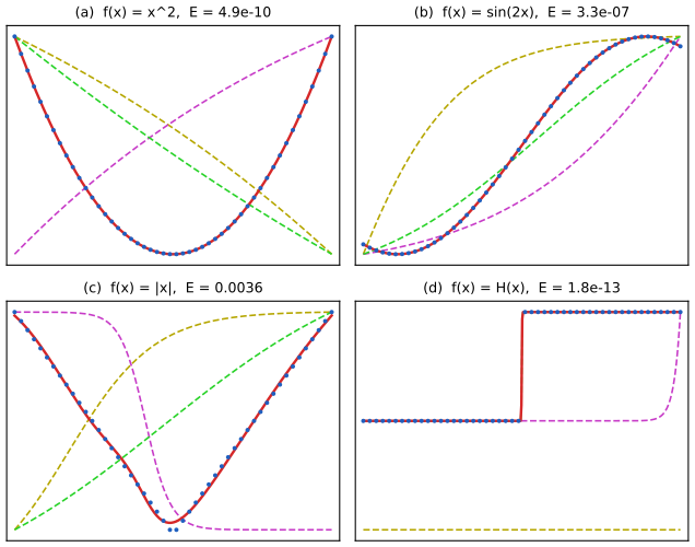
fig5_3. Download: PDF · SVG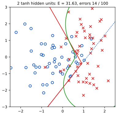
fig5_4. Download: PDF · SVG5.1.1 Weight-space symmetries
pp. 231–232 Different weight vectors can define the very same function \(\mathbf{x}\mapsto\mathbf{y}\). This does not matter for prediction, but it matters for the Bayesian model comparison of Section 5.7, where the volume of weight space occupied by a network enters the evidence.
Result 5.2 (sign-flip and interchange symmetries) pp. 231–232
Consider the two-layer network (5.9) with \(h=\tanh\) and \(M\) hidden units. For a sign vector \(\mathbf{s}\in\{\pm1\}^M\) and a permutation \(\pi\) of \(\{1,\dots,M\}\) define new weights by
\[ \widetilde{w}^{(1)}_{ji}=s_j\,w^{(1)}_{\pi(j)i}\quad(i=0,\dots,D),\qquad \widetilde{w}^{(2)}_{kj}=s_j\,w^{(2)}_{k\pi(j)}\quad(j\ge1),\qquad \widetilde{w}^{(2)}_{k0}=w^{(2)}_{k0}. \]Then the network function is unchanged. These \(2^MM!\) transformations form a group, and for every weight vector outside a null set (one with all first-layer rows non-zero and pairwise different up to sign) they produce \(2^MM!\) distinct weight vectors. So each such \(\mathbf{w}\) belongs to a family of exactly \(M!\,2^M\) equivalent weight vectors; for a network with more than one layer of hidden units the factors of the layers multiply.
Proof
Invariance. Because \(\tanh\) is odd, \(\tanh(s_ja)=s_j\tanh a\) for \(s_j=\pm1\). Hence for each output \[ \sum_{j=1}^{M}\widetilde{w}^{(2)}_{kj}\tanh\Big(\sum_i\widetilde{w}^{(1)}_{ji}x_i\Big)=\sum_{j}s_jw^{(2)}_{k\pi(j)}\,s_j\tanh\Big(\sum_iw^{(1)}_{\pi(j)i}x_i\Big)=\sum_{j}w^{(2)}_{k\pi(j)}\tanh\Big(\sum_iw^{(1)}_{\pi(j)i}x_i\Big), \] because \(s_j^2=1\), and the last sum is the original one with the terms re-ordered (\(\pi\) is a bijection). The output bias is untouched.
Group and count. Composition of two such transformations is another one (compose the permutations and multiply the signs along them), the identity is \((\mathbf{1},\mathrm{id})\) and each element has an inverse, so we have a group \(G\) with \(|G|=2^M\cdot M!\) elements, acting on weight space.
Distinctness. Let \(\mathbf{u}_j=(w^{(1)}_{j0},\dots,w^{(1)}_{jD})\) be the rows of the first layer and assume \(\mathbf{u}_j\ne\mathbf{0}\) and \(\mathbf{u}_j\ne\pm\mathbf{u}_{j'}\) for \(j\ne j'\). Suppose \((\mathbf{s},\pi)\) fixes \(\mathbf{w}\), i.e. \(s_j\mathbf{u}_{\pi(j)}=\mathbf{u}_j\) for all \(j\). If \(\pi(j)\ne j\) this gives \(\mathbf{u}_j=\pm\mathbf{u}_{\pi(j)}\), contradicting the assumption, so \(\pi=\mathrm{id}\); then \(s_j\mathbf{u}_j=\mathbf{u}_j\) with \(\mathbf{u}_j\ne\mathbf{0}\) forces \(s_j=+1\). So only the identity fixes \(\mathbf{w}\) (the action is free there), and \(g\mathbf{w}=g'\mathbf{w}\) implies \(g^{-1}g'\mathbf{w}=\mathbf{w}\), hence \(g=g'\): the orbit has exactly \(|G|\) points. The excluded weights (a zero row, or two rows equal up to sign) form a set of Lebesgue measure zero; there the symmetry is "accidental" and the orbit is smaller. ∎
Remarks. (i) For the logistic sigmoid, \(\sigma(-a)=1-\sigma(a)\), so the sign flip of unit \(j\) is compensated by \(\widetilde{w}^{(2)}_{kj}=-w^{(2)}_{kj}\) together with the output bias shift \(\widetilde{w}^{(2)}_{k0}\)
Filling the gap 5.2: \(\tanh\) and logistic hidden units are equivalent (Exercise 5.1) p. 284
Since \(\sigma(a)=\tfrac12\big(1+\tanh(a/2)\big)\), a network with logistic hidden units equals one with \(\tanh\) hidden units whose parameters differ by linear transformations.
Derivation
\(\tanh(a/2)\)
5.2 Network training
pp. 232–241 The simplest recipe for choosing \(\mathbf{w}\) is the curve-fitting one of Section 1.1: minimise the sum of squares \(E(\mathbf{w})\)
Result 5.3 (error functions as negative log likelihoods) pp. 232–236, (5.12)–(5.25)
Let the data be i.i.d. and write \(y_n=y(\mathbf{x}_n,\mathbf{w})\), \(y_{nk}=y_k(\mathbf{x}_n,\mathbf{w})\).
- Regression. With \(p(t\given\mathbf{x},\mathbf{w})\)
\({}=\N(t\given y(\mathbf{x},\mathbf{w}),\beta^{-1})\) (5.12), minus the log likelihood is \[ \frac\beta2\sum_{n=1}^{N}\{y(\mathbf{x}_n,\mathbf{w})-t_n\}^2-\frac N2\ln\beta+\frac N2\ln(2\pi), \tag{5.13} \] so \(\mathbf{w}_{\rm ML}\) minimises the sum-of-squares error \(E(\mathbf{w})=\tfrac12\sum_n\{y_n-t_n\}^2\) (5.14), and then \[ \frac1{\beta_{\rm ML}}=\frac1N\sum_{n=1}^{N}\{y(\mathbf{x}_n,\mathbf{w}_{\rm ML})-t_n\}^2 . \tag{5.15} \] For \(K\) targets, independent given \(\mathbf{x}\) with common precision, \(p(\mathbf{t}\given\mathbf{x},\mathbf{w})\) \({}=\N(\mathbf{t}\given\mathbf{y}(\mathbf{x},\mathbf{w}),\beta^{-1}\mathbf{I})\) (5.16); \(\mathbf{w}_{\rm ML}\) minimises (5.11) and \(1/\beta_{\rm ML}\) \({}=\frac1{NK}\sum_n\|\mathbf{y}(\mathbf{x}_n,\mathbf{w}_{\rm ML})\) \({}-\mathbf{t}_n\|^2\) (5.17). - One binary target (\(t\in\{0,1\}\), \(y=\sigma(a)=p(\mathcal{C}_1\given\mathbf{x})\), (5.19)): \(p(t\given\mathbf{x},\mathbf{w})=y^t(1-y)^{1-t}\) (5.20) and the cross-entropy error is \[ E(\mathbf{w})=-\sum_{n=1}^{N}\{t_n\ln y_n+(1-t_n)\ln(1-y_n)\}. \tag{5.21} \]
- \(K\) independent binary targets with \(y_k=\sigma(a_k)\): \(p(\mathbf{t}\given\mathbf{x},\mathbf{w})\)
\({}=\prod_ky_k^{t_k}(1-y_k)^{1-t_k}\) (5.22) and \[ E(\mathbf{w})=-\sum_{n=1}^{N}\sum_{k=1}^{K}\{t_{nk}\ln y_{nk}+(1-t_{nk})\ln(1-y_{nk})\}. \tag{5.23} \] - Multiclass (1-of-\(K\) coding, \(y_k=p(t_k=1\given\mathbf{x})\)): \[ E(\mathbf{w})=-\sum_{n=1}^{N}\sum_{k=1}^{K}t_{nk}\ln y_k(\mathbf{x}_n,\mathbf{w}), \tag{5.24} \] with the softmax \(y_k=\exp(a_k)/\sum_j\exp(a_j)\) (5.25). Erratum. The book prints \(t_{kn}\) in (5.24); the index order above is the corrected one.
Derivation (Exercises 5.2 and 5.5, and the choice of \(\beta_{\rm ML}\))
(1) By independence, \(-\ln p(\mathbf{t}\given\mathbf{X},\mathbf{w},\beta)\)
(2)–(3) Take \(-\ln\) of the product over \(n\) of (5.20) and (5.22). Because the first layer is shared, the \(K\) problems are coupled through \(\mathbf{w}\) (the hidden units are shared features), unlike \(K\) separate linear classifiers.
(4) With 1-of-\(K\) targets, \(p(\mathbf{t}\given\mathbf{x})=\prod_ky_k^{t_k}\) (exactly one \(t_k\) is 1), so \(-\ln\prod_n\prod_ky_{nk}^{t_{nk}}\) is (5.24). The softmax is invariant to adding a constant \(c\) to every \(a_k\) (numerator and denominator both pick up \(e^c\)), so \(E\) is constant along these directions of weight space; a regulariser (Section 5.5) removes the degeneracy. ∎
Filling the gap 5.3: correlated targets, noisy labels and \(\pm1\) targets (Exercises 5.3, 5.4, 5.9) pp. 233, 284
The book remarks that "the assumption of independence can be dropped", that the cross-entropy model "is easily extended to allow for labelling errors", and asks for the version with targets \(\pm1\). Here are the three results.
Derivation
Unknown noise covariance (Exercise 5.3). Let \(p(\mathbf{t}\given\mathbf{x},\mathbf{w})\)
Label noise (Exercise 5.4). Suppose the recorded label equals the true one with probability \(1-\epsilon\) and is flipped with probability \(\epsilon\). Then \(P(t=1\given\mathbf{x})\)
Targets \(\pm1\) (Exercise 5.9). Let \(t=1\) for \(\mathcal{C}_1\), \(t=-1\) for \(\mathcal{C}_2\), and \(y\in[-1,1]\). Interpret \(p(\mathcal{C}_1\given\mathbf{x})=(1+y)/2\), \(p(\mathcal{C}_2\given\mathbf{x})=(1-y)/2\). Then \[ E(\mathbf{w})=-\sum_n\Big\{\frac{1+t_n}2\ln\frac{1+y_n}2+\frac{1-t_n}2\ln\frac{1-y_n}2\Big\}. \] This is (5.21) with \(y\to(1+y)/2\), \(t\to(1+t)/2\). The appropriate output nonlinearity is the one that maps the activation to \((-1,1)\) in the canonical way: if \((1+y)/2=\sigma(a)\), then \(y=2\sigma(a)-1=\tanh(a/2)\) (the identity of Filling the gap 5.2). ∎
Result 5.4 (canonical link: the output error signal is \(y_k-t_k\)) pp. 233–236, (5.18)
For each of the three pairings of Result 5.3 (identity with sum of squares, logistic sigmoid with cross-entropy, softmax with multiclass cross-entropy), the derivative of the error of one pattern with respect to the activation of output unit \(k\) is \[ \frac{\partial E_n}{\partial a_k}=y_k-t_k. \tag{5.18} \]
Proof (Exercises 5.6 and 5.7)
Identity. \(E_n=\tfrac12\sum_k(y_k-t_k)^2\) and \(y_k=a_k\), so \(\partial E_n/\partial a_k=y_k-t_k\).
Sigmoid. \(\sigma'(a)=\sigma(a)(1-\sigma(a))\) (differentiate \(\sigma=(1+e^{-a})^{-1}\): \(\sigma'=e^{-a}/(1+e^{-a})^2=\sigma\,(1-\sigma)\)). With \(E_n=-\sum_k\{t_k\ln y_k+(1-t_k)\ln(1-y_k)\}\) and \(y_k=\sigma(a_k)\) only the \(k\)th term depends on \(a_k\): \[ \frac{\partial E_n}{\partial a_k}=-\Big\{\frac{t_k}{y_k}-\frac{1-t_k}{1-y_k}\Big\}y_k(1-y_k)=-t_k(1-y_k)+(1-t_k)y_k=y_k-t_k. \]
Softmax. From \(y_k=e^{a_k}/\sum_je^{a_j}\), \(\partial y_k/\partial a_l=y_k(\delta_{kl}-y_l)\) (the quotient rule: \(\delta_{kl}y_k-y_ky_l\)). With \(E_n=-\sum_kt_k\ln y_k\), \[ \frac{\partial E_n}{\partial a_l}=-\sum_kt_k\frac1{y_k}\,y_k(\delta_{kl}-y_l)=-t_l+y_l\sum_kt_k=y_l-t_l,\] using \(\sum_kt_k=1\) for 1-of-\(K\) coding. ∎
Why it is not an accident. Each pairing is a generalised linear model with an exponential-family noise model in the natural parameter \(a\): \(-\ln p(t\given a)=A(a)-ta+\const\), so \(\partial E/\partial a=A'(a)-t\), and \(A'(a)=\E[t]=y\) is the mean, i.e. the canonical response function (toolkit, Section 4.3.6). For two classes, a single sigmoid output and a two-output softmax coincide: \(y_1=e^{a_1}/(e^{a_1}+e^{a_2})=\sigma(a_1-a_2)\).
5.2.1 Parameter optimization
pp. 236–237 Think of \(E(\mathbf{w})\) as a surface over weight space (Figure 5.5). For a small step, \(\delta E\)
5.2.2 Local quadratic approximation
pp. 237–239 Expanding about a point \(\widehat{\mathbf{w}}\) to second order,
\[ E(\mathbf{w})\simeq E(\widehat{\mathbf{w}})+(\mathbf{w}-\widehat{\mathbf{w}})^\T\mathbf{b}+\tfrac12(\mathbf{w}-\widehat{\mathbf{w}})^\T\mathbf{H}(\mathbf{w}-\widehat{\mathbf{w}}), \tag{5.28} \]
where the gradient \(\mathbf{b}\)
Result 5.5 (geometry near a minimum) pp. 238–239, (5.32)–(5.40)
Let \(\mathbf{w}^\star\) be a stationary point and \(\mathbf{H}\) the (symmetric) Hessian there, with orthonormal eigenvectors \(\mathbf{u}_i\), \(\mathbf{H}\mathbf{u}_i=\lambda_i\mathbf{u}_i\) (5.33), (5.34). In the quadratic approximation, with \(\mathbf{w}-\mathbf{w}^\star\)
- \(E(\mathbf{w})\)
\({}\simeq E(\mathbf{w}^\star)\) \({}+\tfrac12(\mathbf{w}-\mathbf{w}^\star)^\T\mathbf{H}(\mathbf{w}-\mathbf{w}^\star)\) \({}=E(\mathbf{w}^\star)\) \({}+\tfrac12\sum_i\lambda_i\alpha_i^2\) (5.32), (5.36). - \(\mathbf{H}\) is positive definite, \(\mathbf{v}^\T\mathbf{H}\mathbf{v}>0\) for all \(\mathbf{v}\ne\mathbf{0}\) (5.37), if and only if all \(\lambda_i>0\); for \(\mathbf{v}=\sum_ic_i\mathbf{u}_i\), \(\mathbf{v}^\T\mathbf{H}\mathbf{v}\)
\({}=\sum_ic_i^2\lambda_i\) (5.39). - The contours \(E=E(\mathbf{w}^\star)+c\) (\(c>0\)) are ellipsoids centred at \(\mathbf{w}^\star\) with axes along the \(\mathbf{u}_i\) and semi-axis lengths \(\sqrt{2c/\lambda_i}\), inversely proportional to \(\sqrt{\lambda_i}\) (Figure 5.6).
- If \(\mathbf{H}\) is positive definite, \(\mathbf{w}^\star\) is a strict local minimum; if some \(\lambda_i<0\) it is not a minimum (in one dimension the condition is \(\partial^2E/\partial w^2>0\), (5.40)). If the smallest eigenvalue is zero the quadratic model is flat in that direction and higher-order terms decide.
Proof (Exercises 5.10, 5.11, 5.12)
(1) Substitute (5.35) into (5.32): \((\mathbf{w}-\mathbf{w}^\star)^\T\mathbf{H}(\mathbf{w}-\mathbf{w}^\star)\)
(2) The eigenvectors of a symmetric matrix are a complete orthonormal basis, so every \(\mathbf{v}\) is \(\sum c_i\mathbf{u}_i\) with \(c_i=\mathbf{u}_i^\T\mathbf{v}\) (5.38), and the computation of (1) gives (5.39). If all \(\lambda_i>0\), \(\sum c_i^2\lambda_i>0\) unless every \(c_i=0\), i.e. \(\mathbf{v}=\mathbf{0}\). Conversely, taking \(\mathbf{v}=\mathbf{u}_i\) in (5.37) gives \(\mathbf{u}_i^\T\mathbf{H}\mathbf{u}_i\)
(3) The set \(\tfrac12\sum_i\lambda_i\alpha_i^2=c\) is \(\sum_i\alpha_i^2/(2c/\lambda_i)=1\): an ellipsoid with semi-axis \(\sqrt{2c/\lambda_i}\) along \(\mathbf{u}_i\) when all \(\lambda_i>0\). The direction of smallest curvature has the longest axis (the error changes slowest there).
(4) By (1), \(E-E(\mathbf{w}^\star)\)
5.2.3 Use of gradient information
pp. 239–240
Filling the gap 5.4: \(W(W+3)/2\) parameters and the \(O(W^3)\) versus \(O(W^2)\) argument (Exercise 5.13) p. 239
Derivation
The quadratic (5.28) is specified by \(\mathbf{b}\) (\(W\) numbers) and the symmetric \(\mathbf{H}\): a symmetric \(W\times W\) matrix is determined by its diagonal and the entries above it, \(W+\tfrac{W(W-1)}2=\tfrac{W(W+1)}2\) numbers. In total \(W+\tfrac{W(W+1)}2=\tfrac{W(W+3)}2=O(W^2)\) independent elements; the location of the minimum \(\widehat{\mathbf{w}}-\mathbf{H}^{-1}\mathbf{b}\) depends on all of them.
Without gradients. Each function evaluation returns one number and costs \(O(W)\) operations (one forward sweep touches every weight once), and \(O(W^2)\) numbers are needed, so \(O(W^2)\) evaluations of \(O(W)\) each: \(O(W^3)\). With gradients. A gradient evaluation delivers \(W\) numbers, so \(O(W)\) of them suffice, and by backpropagation (Section 5.3) each costs \(O(W)\): in total \(O(W^2)\). This heuristic count is the reason all practical training algorithms use \(\nabla E\). ∎
5.2.4 Gradient descent optimization
pp. 240–241 The simplest use of \(\nabla E\) is a step of size \(\eta>0\) (the learning rate) against the gradient, \[ \mathbf{w}^{(\tau+1)}=\mathbf{w}^{(\tau)}-\eta\nabla E(\mathbf{w}^{(\tau)}). \tag{5.41} \] This is a batch method: each step needs the gradient over the whole training set. When the error is a sum over data points, \[ E(\mathbf{w})=\sum_{n=1}^{N}E_n(\mathbf{w}), \tag{5.42} \] the on-line (sequential, stochastic) version updates after each point, \[ \mathbf{w}^{(\tau+1)}=\mathbf{w}^{(\tau)}-\eta\nabla E_n(\mathbf{w}^{(\tau)}), \tag{5.43} \] cycling through the data or sampling with replacement.
Algorithm 5.1 (gradient descent, batch and on-line) pp. 240–241
- Choose \(\mathbf{w}^{(0)}\) (small random values; several restarts) and \(\eta>0\).
- Batch: compute \(\nabla E=\sum_n\nabla E_n\) by backpropagation (Algorithm 5.2) and set \(\mathbf{w}\leftarrow\mathbf{w}-\eta\nabla E\). On-line: pick a point \(n\), compute \(\nabla E_n\) and set \(\mathbf{w}\leftarrow\mathbf{w}-\eta\nabla E_n\).
- Stop when \(\|\nabla E\|\) is small or the validation error stops improving (Section 5.5.2).
Why on-line methods cope with redundancy. Duplicate every data point: the error doubles, \(2E\), and so does the batch gradient (twice the work for the same direction), while a sweep of on-line updates simply sees each point twice at no extra cost per update. A stationary point of \(E\) is generally not stationary for the individual \(E_n\) (their gradients cancel only in the sum), so on-line updates keep moving and can leave a shallow local minimum. Plain steepest descent is nonetheless a poor batch algorithm (Bishop and Nabney, 2008): its behaviour on the elongated bowls of Result 5.5 is analysed in Result 5.13 (it converges only for \(\eta<2/\lambda_{\max}\) and slowly along directions with small \(\lambda_i\)), while conjugate gradients and quasi-Newton methods decrease the error monotonically and are faster. The demo weight decay and early stopping show the effect of the learning dynamics on fit.
5.3 Error backpropagation
pp. 241–249 Gradient-based training needs \(\nabla E\) at every step, so its cost matters. Backpropagation evaluates all the partial derivatives by passing information forwards and then backwards through the network, at a cost comparable to a single forward evaluation. The word is used loosely in the literature (for the MLP itself, or for gradient descent on the sum of squares). Here it names only the first of the two stages of a training step, the evaluation of derivatives; the second stage, using the derivatives to change the weights, can be done by any optimiser of Section 5.2. The same derivative-propagation idea also yields the Jacobian (5.3.4) and the Hessian (5.4).
5.3.1 Evaluation of error-function derivatives
pp. 242–245 For i.i.d. data the error is a sum over patterns, \[ E(\mathbf{w})=\sum_{n=1}^{N}E_n(\mathbf{w}) , \tag{5.44} \] so it is enough to compute \(\nabla E_n\) for one pattern (and sum, (5.57)). As a warm-up, for a single linear layer \(y_k=\sum_iw_{ki}x_i\) (5.45) with \(E_n=\tfrac12\sum_k(y_{nk}-t_{nk})^2\) (5.46), \[ \frac{\partial E_n}{\partial w_{ji}}=(y_{nj}-t_{nj})\,x_{ni}, \tag{5.47} \] an "error signal" at the output end of the link times the variable at its input end. Backpropagation shows that the same local structure persists in any feed-forward network.
Result 5.6 (backpropagation formulae) pp. 242–245, (5.48)–(5.57)
In a feed-forward network each unit \(j\) forms \(a_j=\sum_iw_{ji}z_i\) (5.48) from the outputs \(z_i\) of the units (or inputs) \(i\) that send it a connection, and outputs \(z_j=h(a_j)\) (5.49). Define the error (or "delta") of unit \(j\) for one pattern as \(\delta_j\equiv\partial E_n/\partial a_j\) (5.51). Then
\[ \frac{\partial E_n}{\partial w_{ji}}=\delta_j\,z_i, \tag{5.53} \]for output units with the canonical link \(\delta_k=y_k-t_k\) (5.54) (Result 5.4), and for every non-output unit \(j\),
\[ \delta_j=h'(a_j)\sum_kw_{kj}\,\delta_k, \tag{5.56} \]the sum running over all units \(k\) to which \(j\) sends a connection. The total derivative is \(\partial E/\partial w_{ji}\)
Proof (the chain rule, step by step)
Fix a pattern and drop the index \(n\). All the \(a\)'s and \(z\)'s are functions of the weights through the forward pass.
(5.50)–(5.53). The weight \(w_{ji}\) enters the forward pass only in the sum \(a_j\), so \(E\) depends on \(w_{ji}\) only through \(a_j\) and \[ \frac{\partial E}{\partial w_{ji}}=\frac{\partial E}{\partial a_j}\frac{\partial a_j}{\partial w_{ji}}\tag{5.50}. \] By the definition (5.51) the first factor is \(\delta_j\); by (5.48) the second is \(\partial a_j/\partial w_{ji}=z_i\) (5.52) (with \(z_i=1\) for a bias). Substituting gives (5.53).
(5.54). For an output unit with canonical link this is Result 5.4. (For another output activation \(y_k=f(a_k)\) and \(E_n\) a function of \(\mathbf{y}\), the chain rule gives \(\delta_k=f'(a_k)\,\partial E_n/\partial y_k\).)
(5.55)–(5.56). A hidden unit \(j\) influences the error only through the units \(k\) it feeds, because the only place \(a_j\) appears downstream is in the \(a_k\) of those units, \(a_k=\sum_{j'}w_{kj'}z_{j'}\ni w_{kj}h(a_j)\). Variations of \(a_j\) therefore change \(E\) only through variations of the \(a_k\): \[ \delta_j=\frac{\partial E}{\partial a_j}=\sum_k\frac{\partial E}{\partial a_k}\frac{\partial a_k}{\partial a_j}=\sum_k\delta_k\frac{\partial a_k}{\partial a_j}\tag{5.55}. \] Now \(\partial a_k/\partial a_j=w_{kj}\,h'(a_j)\) holds for the direct dependence: \(a_k=\sum_{j'}w_{kj'}h(a_{j'})\) contains \(a_j\) only in the term \(w_{kj}h(a_j)\). Nothing is lost by using only the direct dependence, because \(\delta_k=\partial E/\partial a_k\) is a total derivative that already accounts for everything downstream of \(a_k\), and every path from \(a_j\) to the error leaves \(j\) through one of the units \(k\) that it feeds. This gives (5.56).
Order of evaluation. Because the graph has no directed cycle, its units can be ordered so that every unit comes after the units that feed it (a topological order). Forward propagation visits them in this order; \(\delta\) for the outputs is known from (5.54), and (5.56) computes \(\delta_j\) from the \(\delta_k\) of units later in the order, so visiting units in the reverse order evaluates every \(\delta\). Note that (5.56) sums over the first index of \(w_{kj}\) (units above \(j\)), whereas forward propagation (5.10) sums over the second.
If different units have different activation functions, use \(h_j\) in (5.56). ∎
Algorithm 5.2 (error backpropagation) p. 244
- Forward. Apply \(\mathbf{x}_n\) and compute the activations \(a_j\) and outputs \(z_j\) of all hidden and output units by (5.48), (5.49).
- Output errors. Compute \(\delta_k\) for all output units, (5.54).
- Backward. Compute \(\delta_j\) for every hidden unit by (5.56), in reverse topological order.
- Derivatives. \(\partial E_n/\partial w_{ji}=\delta_jz_i\), (5.53). For a batch method, sum over \(n\), (5.57).
5.3.2 A simple example
pp. 245–246 Take the two-layer network of Figure 5.1 with \(\tanh\) hidden units, linear outputs and \(E_n=\tfrac12\sum_k(y_k-t_k)^2\) (5.61). The hidden activation is
\[ h(a)=\tanh a=\frac{e^{a}-e^{-a}}{e^{a}+e^{-a}} \tag{5.58, 5.59} \]
and its derivative is a function of its value (Erratum: "logistic sigmoid" on p. 245 should read "sigmoidal"),
\[ h'(a)=1-h(a)^2. \tag{5.60} \]
Write \(\tanh a=N/D\) with \(N=e^a-e^{-a}\), \(D=e^a+e^{-a}\); then \(N'=D\) and \(D'=N\), so \((N/D)'=(D^2-N^2)/D^2=1-(N/D)^2\), because \(D^2-N^2=4\). The logistic sigmoid satisfies \(\sigma'=\sigma(1-\sigma)\) (Result 5.4), and via \(\tanh a=2\sigma(2a)-1\) the two statements are the same: \(\tfrac{d}{da}\tanh a\)Derivation of (5.60) (Exercise 5.8)
For each pattern, forward propagation is \[ a_j=\sum_{i=0}^{D}w^{(1)}_{ji}x_i,\qquad z_j=\tanh(a_j),\qquad y_k=\sum_{j=0}^{M}w^{(2)}_{kj}z_j, \tag{5.62, 5.63, 5.64} \] then the output errors \(\delta_k=y_k-t_k\) (5.65), the hidden errors \[ \delta_j=(1-z_j^2)\sum_{k=1}^{K}w^{(2)}_{kj}\delta_k, \tag{5.66} \] and the derivatives \[ \frac{\partial E_n}{\partial w^{(1)}_{ji}}=\delta_jx_i,\qquad \frac{\partial E_n}{\partial w^{(2)}_{kj}}=\delta_kz_j. \tag{5.67} \] Note that (5.66) is (5.56) with \(h'(a_j)=1-z_j^2\) computed from the stored forward values \(z_j\), at no extra cost.
Filling the gap 5.5: skip-layer connections and tied weights (Exercises 5.18 and 5.28) pp. 249, 269, 285, 289
Derivation
Skip-layer connections (Exercise 5.18). Add weights \(w^{(\rm skip)}_{ki}\) from input \(x_i\) straight to output \(k\): \(y_k\)
Tied weights (Exercise 5.28). If several weights are constrained to the same value, \(w_{r}=w_{s}=\dots=\omega\), the error is a function of the single parameter \(\omega\) and the chain rule gives \(\partial E/\partial\omega\)
5.3.3 Efficiency of backpropagation
pp. 246–247 Let \(W\) be the number of weights and biases. Forward propagation costs \(O(W)\): except for very sparse networks \(W\) far exceeds the number of units, so the cost is dominated by the multiply-adds of the sums (5.48), and the evaluation of the activation functions is a small overhead. Backpropagation does the same amount of work in reverse: (5.56) uses each weight once, and (5.53) once more, so the whole gradient costs \(O(W)\), only a small constant factor more than evaluating the error itself.
Filling the gap 5.6: finite differences and why they cost \(O(W^2)\) (Exercise 5.14) pp. 246–247, (5.68), (5.69)
An alternative to backpropagation perturbs each weight in turn: \[ \frac{\partial E_n}{\partial w_{ji}}=\frac{E_n(w_{ji}+\epsilon)-E_n(w_{ji})}\epsilon+O(\epsilon), \tag{5.68} \] \[ \frac{\partial E_n}{\partial w_{ji}}=\frac{E_n(w_{ji}+\epsilon)-E_n(w_{ji}-\epsilon)}{2\epsilon}+O(\epsilon^2). \tag{5.69} \]
Derivation, the cost, and a gradient check
Taylor expansion. Write \(f(\epsilon)=E_n(w_{ji}+\epsilon)\) with all other weights fixed. Then \(f(\pm\epsilon)\)
Cost. Each quotient needs forward passes costing \(O(W)\), and there are \(W\) weights to perturb: \(O(W^2)\) in total instead of backpropagation's \(O(W)\). In floating point the truncation error \(\propto\epsilon^2\) must be balanced against the rounding error \(\propto u/\epsilon\) (\(u\approx10^{-16}\)), so the best central difference uses \(\epsilon\approx u^{1/3}\sim10^{-5}\) and is accurate to about \(u^{2/3}\sim10^{-10}\) relative.
A gradient check (the use that matters). Numerical differentiation is far too slow for training but is the standard test of a backpropagation implementation. I ran it on a small network (\(D=2\), \(M=3\), \(K=2\) \(\tanh\)/linear, \(W=17\) weights and biases, \(N=6\) random patterns, weights drawn from \(\N(0,0.7^2)\), seed 1) with the formulae (5.62)–(5.67):
| \(\epsilon\) | \(10^{-1}\) | \(10^{-2}\) | \(10^{-3}\) | \(10^{-4}\) | \(10^{-5}\) | \(10^{-6}\) | \(10^{-8}\) |
|---|---|---|---|---|---|---|---|
| max error, forward difference (5.68) | 3.0e-1 | 3.0e-2 | 3.0e-3 | 3.0e-4 | 3.0e-5 | 3.0e-6 | 4.5e-7 |
| max error, central difference (5.69) | 2.8e-3 | 2.8e-5 | 2.8e-7 | 2.8e-9 | 1.7e-10 | 2.3e-9 | 2.8e-7 |
The errors are the largest absolute difference over the 17 components against the backpropagation gradient (whose largest component is 12.5). The forward difference falls like \(\epsilon\), the central one like \(\epsilon^2\), until rounding error takes over below \(\epsilon\approx10^{-5}\): exactly the behaviour derived above, and the agreement to \(1.7\times10^{-10}\) confirms (5.66), (5.67) including the bias terms. The preset Backprop gradient against finite differences shows the same comparison interactively.
def grad(w):                       # backpropagation, (5.62)-(5.67), summed over patterns
    for x, t in zip(X, T):
        xe, a, z, ze, y = forward(w, x)          # xe = (1, x), ze = (1, z)
        dk = y - t                                # (5.65)
        dj = (1 - z**2) * (W2[:, 1:].T @ dk)      # (5.66)
        g1 += np.outer(dj, xe); g2 += np.outer(dk, ze)   # (5.67)
num = [(E(w + eps*e) - E(w - eps*e)) / (2*eps) for e in np.eye(W)]   # (5.69)
∎Modular systems and the Jacobian. Backpropagation applies to any differentiable module, not only to sigmoidal layers. In a system built of modules (Figure 5.8: an adaptive module with parameter \(\mathbf{w}\) feeding other modules that produce \(\mathbf{y}\)), the chain rule gives \(\partial E/\partial\mathbf{w}\)
5.3.4 The Jacobian matrix
pp. 247–249 The Jacobian of the network map has entries \[ J_{ki}\equiv\frac{\partial y_k}{\partial x_i}, \tag{5.70} \] each evaluated with the other inputs held fixed. It measures how sensitive the outputs are to the inputs; for small known input errors \(\Delta x_i\), \[ \Delta y_k\simeq\sum_i\frac{\partial y_k}{\partial x_i}\Delta x_i, \tag{5.72} \] valid only locally, because the network is nonlinear and \(\mathbf{J}\) must be re-evaluated at each input.
Result 5.7 (Jacobian by backpropagation) pp. 248–249, (5.73)–(5.77)
With the notation of Result 5.6, \[ J_{ki}=\sum_jw_{ji}\frac{\partial y_k}{\partial a_j}, \tag{5.73} \] the sum running over all units \(j\) that the input \(i\) feeds, and the derivatives \(\partial y_k/\partial a_j\) obey the backward recursion \[ \frac{\partial y_k}{\partial a_j}=h'(a_j)\sum_lw_{lj}\frac{\partial y_k}{\partial a_l}, \tag{5.74} \] started at the outputs with \[ \frac{\partial y_k}{\partial a_l}=\delta_{kl}\,\sigma'(a_l)\ \text{(sigmoid outputs)}\ (5.75),\qquad \frac{\partial y_k}{\partial a_l}=\delta_{kl}\,y_k-y_ky_l\ \text{(softmax outputs)}\ (5.76). \] Erratum. The book indexes these with \(j\); the index \(l\) above conforms with (5.74). For linear outputs \(\partial y_k/\partial a_l=\delta_{kl}\). Row \(k\) of \(\mathbf{J}\) costs one backward sweep, so the full Jacobian costs \(K\) sweeps, each \(O(W)\).
Proof, the forward alternative (Exercise 5.15), and the check (5.77)
(5.73). The input \(x_i\) affects \(y_k\) only through the activations \(a_j\) of the units it feeds, hence \(J_{ki}\)
(5.74). The same argument as for (5.56), with \(\partial y_k/\partial a_j\)
(5.75), (5.76). For a logistic sigmoid output \(y_k=\sigma(a_k)\) depends only on \(a_k\): \(\partial y_k/\partial a_l\)
Forward alternative (Exercise 5.15). Instead of a backward sweep per output, propagate the sensitivities of every unit to one input \(x_i\) forwards. Put \(\partial x_{i'}/\partial x_i=\delta_{ii'}\) for the inputs and, in topological order, \(\partial a_j/\partial x_i\)
Check (5.77). Central differences \(\partial y_k/\partial x_i\)
5.4 The Hessian matrix
pp. 249–256 Backpropagation also gives second derivatives \(\partial^2E/\partial w_{ji}\partial w_{lk}\) (5.78); collecting all \(W\) parameters in one vector, these are the entries \(H_{ij}\) of the Hessian. The Hessian is used for: (1) second-order optimisation algorithms; (2) fast re-training after a small change of the data; (3) pruning, where the inverse Hessian ranks weights by their importance; (4) the Laplace approximation of Section 5.7, where \(\mathbf{H}^{-1}\) gives the predictive variance, its eigenvalues give the hyperparameters and its determinant the evidence. A \(W\times W\) matrix has \(W^2\) entries, so no method can do better than \(O(W^2)\) per pattern for the whole matrix; the exact algorithm of Section 5.4.5 attains this.
5.4.1 Diagonal approximation
pp. 250 The inverse of a diagonal matrix is trivial, so a diagonal approximation is cheap to invert. Work pattern by pattern (\(E=\sum_nE_n\)).
Result 5.8 (diagonal Hessian elements) p. 250, (5.79)–(5.81)
For one pattern, \[ \frac{\partial^2E_n}{\partial w_{ji}^2}=\frac{\partial^2E_n}{\partial a_j^2}\,z_i^2, \tag{5.79} \] \[ \frac{\partial^2E_n}{\partial a_j^2}=h'(a_j)^2\sum_k\sum_{k'}w_{kj}w_{k'j}\frac{\partial^2E_n}{\partial a_k\partial a_{k'}}+h''(a_j)\sum_kw_{kj}\frac{\partial E_n}{\partial a_k}, \tag{5.80} \] where \(k,k'\) run over the units fed by \(j\). Neglecting the off-diagonal second derivatives \(k\ne k'\) gives the recursion \[ \frac{\partial^2E_n}{\partial a_j^2}\simeq h'(a_j)^2\sum_kw_{kj}^2\frac{\partial^2E_n}{\partial a_k^2}+h''(a_j)\sum_kw_{kj}\frac{\partial E_n}{\partial a_k}, \tag{5.81} \] which costs \(O(W)\). Erratum. The official errata correct a typographical error in the derivative in the last term of (5.80); the form above is the one the derivation gives.
Proof
(5.79): \(E_n\) depends on \(w_{ji}\) only through \(a_j=\sum_iw_{ji}z_i\), with \(\partial a_j/\partial w_{ji}=z_i\) independent of \(w_{ji}\); so \(\partial^2E_n/\partial w_{ji}^2\)
(5.80): start from (5.56), \(\delta_j\)
(5.81): keep only \(k=k'\) in the double sum. The result is a backward recursion of the same shape as (5.56), started at the output units with \(\partial^2E_n/\partial a_k^2\) (equal to 1 for linear outputs and the sum of squares). ∎
Ricotti et al. (1988) keep all terms in (5.80), which makes the diagonal exact but the cost no longer \(O(W)\). In practice the Hessian of a trained network is strongly non-diagonal, so diagonal approximations driven by convenience must be used with care.
5.4.2 Outer product approximation
pp. 251 For regression with a single output and \(E=\tfrac12\sum_n(y_n-t_n)^2\) (5.82) the Hessian is \[ \mathbf{H}=\nabla\nabla E=\sum_{n=1}^{N}\nabla y_n(\nabla y_n)^\T+\sum_{n=1}^{N}(y_n-t_n)\nabla\nabla y_n. \tag{5.83} \] Erratum. The book omits the transpose in the first term. Dropping the second term gives the Levenberg–Marquardt or outer product approximation \[ \mathbf{H}\simeq\sum_{n=1}^{N}\mathbf{b}_n\mathbf{b}_n^\T,\qquad \mathbf{b}_n\equiv\nabla a_n=\nabla y_n . \tag{5.84} \] Erratum. The book writes \(\mathbf{b}_n=\nabla y_n=\nabla a_n\); the order of definition above is the corrected one.
Result 5.9 (outer product approximation: when it is good, other error functions, and its meaning) pp. 251, 286–287, (5.83)–(5.85); Exercises 5.16, 5.17, 5.19, 5.20
- Why the dropped term is small. If \(y_n\approx t_n\) after training, \((y_n-t_n)\nabla\nabla y_n\) is small. More generally, \(y_n-t_n\) has zero mean given \(\mathbf{x}_n\) at the optimal \(y=\E[t\given\mathbf{x}]\) (Section 1.5.5); if it is uncorrelated with \(\nabla\nabla y_n\), the sum over \(n\) averages out.
- Several outputs (Exercise 5.16). \(\mathbf{H}\)
\({}\simeq\sum_n\sum_{k=1}^K\nabla y_{nk}(\nabla y_{nk})^\T\). - Logistic sigmoid with cross-entropy (Exercise 5.19): \(\displaystyle\mathbf{H}\)
\({}\simeq\sum_{n=1}^{N}y_n(1-y_n)\,\mathbf{b}_n\mathbf{b}_n^\T\) (5.85), with \(\mathbf{b}_n=\nabla a_n\). - Softmax with cross-entropy (Exercise 5.20): \(\displaystyle\mathbf{H}\)
\({}\simeq\sum_n\sum_{k,l}y_{nk}(\delta_{kl}-y_{nl})\,\mathbf{b}_{nk}\mathbf{b}_{nl}^\T\), with \(\mathbf{b}_{nk}=\nabla a_{nk}\). - Population version (Exercise 5.17). For \(E\)
\({}=\tfrac12\iint\{y(\mathbf{x},\mathbf{w})\) \({}-t\}^2p(\mathbf{x},t)\,d\mathbf{x}\,dt\) at the minimiser \(y=\E[t\given\mathbf{x}]\), \(\displaystyle\frac{\partial^2E}{\partial w_r\partial w_s}\) \({}=\int\frac{\partial y}{\partial w_r}\frac{\partial y}{\partial w_s}p(\mathbf{x})\,d\mathbf{x}\) (5.194); a finite sample from \(p(\mathbf{x})\) gives (5.84). - Meaning. The matrix in (5.84) is the Gauss–Newton matrix \(\mathbf{J}^\T\mathbf{J}\) of the residuals, positive semi-definite, and under the Gaussian noise model (5.12) it is \(\beta^{-1}\) times the Fisher information; (5.85) and item 4 are the Fisher information of the Bernoulli and categorical models. Its rank is at most \(NK\).
Proof
(5.83). \(\nabla E=\sum_n(y_n-t_n)\nabla y_n\). Differentiating once more by the product rule gives \(\sum_n\nabla y_n(\nabla y_n)^\T\)
(6) Under (5.12), \(\nabla_{\mathbf{w}}\ln p(t\given\mathbf{x},\mathbf{w})\)
Link to Levenberg–Marquardt. Minimising \(\tfrac12\sum_n(y_n(\mathbf{w})-t_n)^2\) by linearising \(y_n(\mathbf{w}+\Delta)\) pp. 252 Write the outer-product approximation as \(\mathbf{H}_N\) For an invertible symmetric \(\mathbf{M}\) and a vector \(\mathbf{v}\) with \(1+\mathbf{v}^\T\mathbf{M}^{-1}\mathbf{v}\ne0\),
\[ (\mathbf{M}+\mathbf{v}\mathbf{v}^\T)^{-1}=\mathbf{M}^{-1}-\frac{(\mathbf{M}^{-1}\mathbf{v})(\mathbf{v}^\T\mathbf{M}^{-1})}{1+\mathbf{v}^\T\mathbf{M}^{-1}\mathbf{v}} . \tag{5.88} \]
Hence, with \(\mathbf{H}_0=\alpha\mathbf{I}\),
\[ \mathbf{H}_{L+1}^{-1}=\mathbf{H}_L^{-1}-\frac{\mathbf{H}_L^{-1}\mathbf{b}_{L+1}\mathbf{b}_{L+1}^\T\mathbf{H}_L^{-1}}{1+\mathbf{b}_{L+1}^\T\mathbf{H}_L^{-1}\mathbf{b}_{L+1}} , \tag{5.89} \]
which after one pass over the data gives \((\mathbf{H}_N+\alpha\mathbf{I})^{-1}\) in \(O(NW^2)\) operations. With \(K\) outputs, treat each pair \((n,k)\) as a separate rank-one term (below). (5.88) is the case of the Woodbury identity (toolkit) with a rank-one update. Direct check: multiply \((\mathbf{M}+\mathbf{v}\mathbf{v}^\T)\) by the right-hand side and write \(\mathbf{u}=\mathbf{M}^{-1}\mathbf{v}\), \(c=1+\mathbf{v}^\T\mathbf{u}\):
\[ (\mathbf{M}+\mathbf{v}\mathbf{v}^\T)\Big(\mathbf{M}^{-1}-\frac{\mathbf{u}\mathbf{u}^\T}{c}\Big)=\mathbf{I}+\mathbf{v}\mathbf{u}^\T-\frac{\mathbf{v}\mathbf{u}^\T}{c}-\frac{\mathbf{v}(\mathbf{v}^\T\mathbf{u})\mathbf{u}^\T}{c}=\mathbf{I}+\mathbf{v}\mathbf{u}^\T\Big[1-\frac{1+\mathbf{v}^\T\mathbf{u}}{c}\Big]=\mathbf{I}. \]
(5.89) is (5.88) with \(\mathbf{M}=\mathbf{H}_L\), \(\mathbf{v}=\mathbf{b}_{L+1}\), where \(\mathbf{H}_L\) is the Hessian of the first \(L\) points plus \(\alpha\mathbf{I}\) and so is invertible; \(c>0\) because \(\mathbf{M}^{-1}\) is positive definite. The start \(\mathbf{H}_0^{-1}=\alpha^{-1}\mathbf{I}\) means the recursion computes the inverse of \(\mathbf{H}_N+\alpha\mathbf{I}\); the result is not sensitive to the small value of \(\alpha\). Each step costs \(O(W^2)\) (matrix-vector product and outer product). Several outputs (Exercise 5.21). The multi-output outer product is \(\sum_n\sum_k\mathbf{b}_{nk}\mathbf{b}_{nk}^\T\) (Result 5.9, item 2), so apply (5.89) once for each pair \((n,k)\) with \(\mathbf{b}_{nk}=\nabla y_{nk}\): \(NK\) updates of cost \(O(W^2)\). For the sigmoid cross-entropy case use \(\mathbf{b}\to\sqrt{y_n(1-y_n)}\,\mathbf{b}_n\); for the softmax, factor the positive semi-definite \(K\times K\) matrix \(\bm\Lambda_n\) Quasi-Newton optimisers (BFGS and relatives) build an approximation to \(\mathbf{H}^{-1}\) as a by-product of training (Bishop and Nabney, 2008). pp. 252–253 Perturbing every pair of weights,
\[ \frac{\partial^2E}{\partial w_{ji}\partial w_{lk}}=\frac1{4\epsilon^2}\{E(w_{ji}+\epsilon,w_{lk}+\epsilon)-E(w_{ji}+\epsilon,w_{lk}-\epsilon)-E(w_{ji}-\epsilon,w_{lk}+\epsilon)+E(w_{ji}-\epsilon,w_{lk}-\epsilon)\}+O(\epsilon^2). \tag{5.90} \]
Applying central differences to the first derivatives, themselves obtained by backpropagation, is cheaper:
\[ \frac{\partial^2E}{\partial w_{ji}\partial w_{lk}}=\frac1{2\epsilon}\Big\{\frac{\partial E}{\partial w_{ji}}(w_{lk}+\epsilon)-\frac{\partial E}{\partial w_{ji}}(w_{lk}-\epsilon)\Big\}+O(\epsilon^2). \tag{5.91} \] Write \(a,b\) for the two weights and expand \(E(w_a+s\epsilon,w_b+t\epsilon)\) with \(s,t=\pm1\) in a Taylor series; the combination in (5.90) is \(\sum_{s,t}st\,E(w_a+s\epsilon,w_b+t\epsilon)\). A monomial \(s^pt^q\) multiplied by \(st\) sums over \(s,t\in\{\pm1\}\) to \(\sum_ss^{p+1}\sum_tt^{q+1}\), which is 4 if both \(p+1\) and \(q+1\) are even and 0 otherwise. The terms of total degree \(d=p+q\): for \(d=0\) (\(p=q=0\)) and \(d=1\) one of \(p+1,q+1\) is odd, so they vanish; for \(d=2\) only \(p=q=1\) survives, with coefficient \(\partial^2E/\partial w_a\partial w_b\,\epsilon^2\) (the cross term of \(\tfrac12(s\epsilon\partial_a+t\epsilon\partial_b)^2\) is \(st\,\epsilon^2E_{ab}\)), giving \(4\epsilon^2E_{ab}\); for odd \(d\) (and in particular \(d=3\)) \(p+1\) and \(q+1\) cannot both be even, so all odd orders vanish. The first neglected term is \(d=4\), \(O(\epsilon^4)\). Dividing by \(4\epsilon^2\) gives \(E_{ab}+O(\epsilon^2)\), which is (5.90). For (5.91), the central quotient (5.69) applied to the function \(w_{lk}\mapsto\partial E/\partial w_{ji}\) has error \(O(\epsilon^2)\). Cost. There are \(W^2\) entries (\(W(W+1)/2\) by symmetry), each needing 4 forward passes of cost \(O(W)\) per pattern: \(O(W^3)\) for (5.90). In (5.91) only the \(W\) weights are perturbed, each time twice evaluating a gradient at \(O(W)\); each perturbation yields a whole row of \(\mathbf{H}\), so the cost is \(O(W^2)\). Both are valuable as checks of a Hessian code. ∎ pp. 253–254 For a network with two layers of weights the exact Hessian is derived by differentiating the backpropagation formulae. Indices \(i,i'\) denote inputs, \(j,j'\) hidden units, \(k,k'\) outputs, and
\[ \delta_k=\frac{\partial E_n}{\partial a_k},\qquad M_{kk'}\equiv\frac{\partial^2E_n}{\partial a_k\partial a_{k'}} . \tag{5.92} \]
(For the sum of squares with linear outputs \(M_{kk'}=\delta_{kk'}\), for sigmoid cross-entropy \(M_{kk'}=\delta_{kk'}y_k(1-y_k)\), for softmax cross-entropy \(M_{kk'}=y_k\delta_{kk'}-y_ky_{k'}\).) If a weight is a bias, set the corresponding \(x_i\) or \(z_j\) to 1. The full Hessian is the sum over patterns and costs \(O(W^2)\). Use (5.53): \(\partial E_n/\partial w^{(2)}_{kj}=\delta_kz_j\) and \(\partial E_n/\partial w^{(1)}_{ji}=\delta_jx_i\), with \(\delta_j=h'(a_j)\sum_kw^{(2)}_{kj}\delta_k\). Two chain-rule facts: \(\partial a_{k'}/\partial w^{(2)}_{kj}\) (5.93). \(z_j\) does not depend on second-layer weights, and \(\delta_k\) depends on \(w^{(2)}_{k'j'}\) through \(a_{k'}\) only: \(\partial\delta_k/\partial w^{(2)}_{k'j'}\) (5.94). Differentiate \(\delta_jx_i\) with respect to \(w^{(1)}_{j'i'}\), which acts through \(a_{j'}\) (factor \(x_{i'}\)): \(x_ix_{i'}\,\partial\delta_j/\partial a_{j'}\). Differentiate \(\delta_j=h'(a_j)\sum_kw^{(2)}_{kj}\delta_k\). The factor \(h'(a_j)\) depends on \(a_{j'}\) only if \(j=j'\), giving \(h''(a_{j'})I_{jj'}\sum_kw^{(2)}_{kj'}\delta_k\) (the first term). Each \(\delta_k\) depends on \(a_{j'}\) through every \(a_{k'}\): \(\partial\delta_k/\partial a_{j'}\) (5.95). Differentiate \(\delta_kz_{j'}\) with respect to \(w^{(1)}_{ji}\): \(z_{j'}\) gives \(h'(a_{j'})I_{jj'}x_i\), and \(\delta_k\) gives \(\sum_{k'}M_{kk'}w^{(2)}_{k'j}h'(a_j)x_i\). Sum: \(x_ih'(a_j)\{\delta_kI_{jj'}\) Skip-layer connections (Exercise 5.23). With \(a_k\) Numerical check. I coded (5.93)–(5.95) (with biases as constant units) for the small network of Section 5.3.3 with the sum of squares (\(M_{kk'}=\delta_{kk'}\)) and compared with the Hessian obtained by central differences of the backpropagated gradient, (5.91): the largest entry-wise difference was \(1.7\times10^{-10}\). ∎ pp. 254–256 Often one needs \(\mathbf{H}\mathbf{v}\) (or \(\mathbf{v}^\T\mathbf{H}\)), not \(\mathbf{H}\): conjugate-gradient or power iterations, trace estimates, eigenvalues for \(\gamma\) (Section 5.7.2). Forming \(\mathbf{H}\) costs \(O(W^2)\) time and storage, but \(\mathbf{v}^\T\mathbf{H}\) has only \(W\) entries, and can be had in \(O(W)\). Since \(\mathbf{H}\) is symmetric,
\[ \mathbf{v}^\T\mathbf{H}=\mathbf{v}^\T\nabla(\nabla E), \tag{5.96} \]
i.e. the directional derivative of the gradient. Define the differential operator \(\mathcal{R}\{\cdot\}\equiv\mathbf{v}^\T\nabla\) (Pearlmutter, 1994); it obeys the ordinary rules of calculus (linearity, product rule, chain rule) and
\[ \mathcal{R}\{\mathbf{w}\}=\mathbf{v}. \tag{5.97} \] Linear outputs, sum-of-squares error, one pattern; \(v_{ji}\) is the component of \(\mathbf{v}\) that belongs to \(w_{ji}\). Why \(\mathcal{R}\{\nabla E\}=\mathbf{v}^\T\mathbf{H}\). The \(r\)th component of \(\mathcal{R}\{\nabla E\}\) is \(\sum_sv_s\,\partial(\partial E/\partial w_r)/\partial w_s\) Rules used. The operator is a first-order derivative, so \(\mathcal{R}\{fg\}\) (5.101)–(5.103). \(\mathcal{R}\{a_j\}\) (5.106), (5.107). \(\mathcal{R}\{\delta_k\}\) (5.110), (5.111). Apply \(\mathcal{R}\) to \(\partial E/\partial w_{kj}=\delta_kz_j\) and \(\partial E/\partial w_{ji}=\delta_jx_i\). Cost. The \(\mathcal{R}\) pass mirrors the ordinary forward and backward passes, with a few extra multiply-adds per weight; the cost is \(O(W)\), a small multiple of the cost of the gradient. Taking \(\mathbf{v}\) to be the unit vectors \((0,\dots,1,\dots,0)\) one at a time gives the columns of \(\mathbf{H}\): \(W\) passes of \(O(W)\), \(O(W^2)\) in total, analytically the same as the algorithm of Section 5.4.5 (Bishop 1992), with some redundant computation. Numerical check. On the small network of Section 5.3.3 (\(W=17\), sum of squares) I computed \(\mathbf{H}\mathbf{v}\) for a random \(\mathbf{v}\) with Algorithm 5.3 and with the Hessian obtained from (5.91): the largest difference over the 17 components was \(2.6\times10^{-10}\), while \(\max|\mathbf{H}\mathbf{v}|=9.9\). A cheap alternative that needs only gradient evaluations is \(\mathbf{H}\mathbf{v}\) pp. 256–272 The numbers of inputs and outputs are fixed by the data, but the number \(M\) of hidden units is free and controls model complexity. One might hope for an optimal \(M\) balancing under- and over-fitting (Figure 5.9), but the generalisation error is not a smooth function of \(M\), because of local minima: Figure 5.10 shows 30 random starts for each \(M\), and the best validation error happened at \(M=8\). An alternative is to take \(M\) large and add a regulariser, the simplest being weight decay
\[ \widetilde{E}(\mathbf{w})=E(\mathbf{w})+\frac\lambda2\mathbf{w}^\T\mathbf{w}, \tag{5.112} \]
the negative log of a zero-mean Gaussian prior with precision \(\lambda\) (Chapter 3). pp. 257–259 Simple weight decay treats all weights alike and is inconsistent with the scaling properties of networks. Take a two-layer network with linear outputs,
\[ z_j=h\Big(\sum_iw_{ji}x_i+w_{j0}\Big),\qquad y_k=\sum_jw_{kj}z_j+w_{k0}, \tag{5.113, 5.114} \]
and rescale the data linearly,
\[ x_i\to\widetilde{x}_i=ax_i+b,\qquad y_k\to\widetilde{y}_k=cy_k+d . \tag{5.115, 5.118} \]
The network mapping is unchanged under the input transformation (5.115) if the first-layer weights and biases are replaced by
\[ \widetilde{w}_{ji}=\frac1a\,w_{ji},\qquad \widetilde{w}_{j0}=w_{j0}-\frac ba\sum_iw_{ji}, \tag{5.116, 5.117} \]
and the output transformation (5.118) is realised by
\[ \widetilde{w}_{kj}=c\,w_{kj},\qquad \widetilde{w}_{k0}=c\,w_{k0}+d. \tag{5.119, 5.120} \]
The regulariser
\[ \frac{\lambda_1}2\sum_{w\in\mathcal{W}_1}w^2+\frac{\lambda_2}2\sum_{w\in\mathcal{W}_2}w^2, \tag{5.121} \]
(\(\mathcal{W}_1,\mathcal{W}_2\): first- and second-layer weights, biases excluded) is invariant under the shifts of the biases, and its value is unchanged under the rescalings (5.116), (5.119) if \(\lambda_1\) and \(\lambda_2\) are rescaled to \(\widetilde\lambda_1=a^{2}\lambda_1\) and \(\widetilde\lambda_2=c^{-2}\lambda_2\). Plain weight decay (5.112) has neither property. First layer. The new hidden activation is \(\widetilde a_j\) Regulariser. Biases do not appear in (5.121), so the bias shifts (5.117), (5.120) change nothing. Under (5.116), \(\sum_{\mathcal{W}_1}\widetilde w^2\) Why plain weight decay fails. \(\lambda\,\mathbf{w}^\T\mathbf{w}\) includes the biases (not invariant to the shift (5.117), which moves \(w_{j0}\)) and weights the two layers equally, while (5.116) and (5.119) multiply the weights of the two layers by different factors \(1/a\) and \(c\): for \(a\ne c^{-1}\)... for any \(a\ne1\) or \(c\ne1\) the regulariser value changes, so training on rescaled data returns a different solution than the rescaled solution. A remark on the printed exponents. The book writes the rescalings as \(\lambda_1\to a^{1/2}\lambda_1\) and \(\lambda_2\to c^{-1/2}\lambda_2\). Following the book's own requirement (the regulariser keeps its value under the weight transformations), the computation above gives the exponents \(2\) and \(-2\); the printed \(1/2\) does not follow, and I could not find it in the official errata list. (If one also demands that the whole sum-of-squares objective is consistent, note that the data term scales by \(c^2\) under (5.118), so the full condition is \(\widetilde\lambda_1=a^2c^2\lambda_1\), \(\widetilde\lambda_2=\lambda_2\); the two forms differ by the overall factor \(c^2\) common to both coefficients.) ∎ The regulariser (5.121) is the negative log of the (improper) prior
\[ p(\mathbf{w}\given\alpha_1,\alpha_2)\propto\exp\Big(-\frac{\alpha_1}2\sum_{w\in\mathcal{W}_1}w^2-\frac{\alpha_2}2\sum_{w\in\mathcal{W}_2}w^2\Big), \tag{5.122} \]
improper because the biases are unconstrained, so it cannot be normalised and its evidence would be zero. For Bayesian model comparison one therefore gives the biases their own Gaussian priors (breaking the shift invariance), leaving four hyperparameters \(\alpha_1^w,\alpha_1^b,\alpha_2^w,\alpha_2^b\). More generally, any partition of the weights into groups \(\mathcal{W}_k\) gives
\[ p(\mathbf{w})\propto\exp\Big(-\frac12\sum_k\alpha_k\|\mathbf{w}\|_k^2\Big),\qquad \|\mathbf{w}\|_k^2=\sum_{j\in\mathcal{W}_k}w_j^2 . \tag{5.123, 5.124} \]
If the groups are the weights leaving each input unit and the \(\alpha_k\) are chosen by maximising the marginal likelihood, this is automatic relevance determination (Section 7.2.2): inputs with large \(\alpha_k\) are switched off. What the four hyperparameters do (a heuristic derivation). The output is \(f(x)\) pp. 259–262 The error on an independent validation set usually falls and then rises as the network begins to over-fit while the training error keeps decreasing; stopping at the minimum of the validation error (Figure 5.12) gives good generalisation. Qualitatively the number of effective degrees of freedom starts small and grows with training. For a quadratic error this can be made precise. Let \(E(\mathbf{w})\) The gradient is \(\nabla E=\mathbf{H}(\mathbf{w}-\mathbf{w}^\star)\). Subtract \(\mathbf{w}^\star\) from the update: \(\mathbf{w}^{(\tau)}-\mathbf{w}^\star\) (a) \((1-\rho\eta_j)^\tau\to0\) iff \(|1-\rho\eta_j|<1\) iff \(0<\rho\eta_j<2\); this holds for all \(j\) iff \(\rho<2/\eta_{\max}\). (b) For \(\rho\eta_j\ll1\), \((1-\rho\eta_j)^\tau\) Rate. The slowest component has factor \(1-\rho\eta_{\min}\) per step, and \(\rho<2/\eta_{\max}\), so the number of steps to fit it is of order \(\eta_{\max}/\eta_{\min}\), the condition number of the Hessian: the reason steepest descent is slow on the long thin valleys of Figure 5.6. pp. 261–263 In many tasks the prediction should not change under transformations of the input: translation or scale of an object in an image, small non-linear time warping in speech. If enough training examples of the transformations are available, an adaptive model can learn the invariance, but the number of combinations grows exponentially with the number of invariances. Four ways to encourage invariance are listed: pp. 263–265 A continuous transformation (translation, rotation, but not reflection) governed by a parameter \(\xi\) moves the input \(\mathbf{x}_n\) along a one-dimensional manifold \(\mathcal{M}\) (Figure 5.15). Let \(\mathbf{s}(\mathbf{x},\xi)\) be the transformed vector, with \(\mathbf{s}(\mathbf{x},0)=\mathbf{x}\). The tangent vector at \(\mathbf{x}_n\) is
\[ \bm\tau_n=\frac{\partial\mathbf{s}(\mathbf{x}_n,\xi)}{\partial\xi}\Big|_{\xi=0}. \tag{5.125} \]
In practice \(\bm\tau_n\) is approximated by a finite difference, \((\mathbf{s}(\mathbf{x}_n,\xi)-\mathbf{x}_n)/\xi\) for a small \(\xi\) (Figure 5.16). Under the transformation, output \(k\) changes at the rate
\[ \frac{\partial y_k}{\partial\xi}\Big|_{\xi=0}=\sum_{i=1}^{D}\frac{\partial y_k}{\partial x_i}\frac{\partial x_i}{\partial\xi}\Big|_{\xi=0}=\sum_{i=1}^{D}J_{ki}\tau_i , \tag{5.126} \]
with \(J_{ki}\) the Jacobian (5.70). The tangent propagation error is \(\widetilde E=E+\lambda\Omega\) (5.127) with
\[ \Omega=\frac12\sum_n\sum_k\Big(\frac{\partial y_{nk}}{\partial\xi}\Big|_{\xi=0}\Big)^2=\frac12\sum_n\sum_k\Big(\sum_{i=1}^{D}J_{nki}\tau_{ni}\Big)^2 . \tag{5.128} \]
It vanishes when the network is locally invariant at every training pattern. Moreover, with the differential operator \(\mathcal{G}\) (5.126) is the chain rule and (5.128) the sum of squares of (5.126). For (5.201), \(\mathcal{G}y_k\) Forward equations. \(\mathcal{G}\) is a first-order differential operator in \(\mathbf{x}\) with the usual chain and product rules, \(\mathcal{G}x_i=\tau_i\), and \(\mathcal{G}w=0\) (weights do not depend on \(\mathbf{x}\)). Apply it to \(a_j=\sum_iw_{ji}z_i\): \(\beta_j=\sum_iw_{ji}\alpha_i\); to \(z_j=h(a_j)\): \(\alpha_j=h'(a_j)\beta_j\). These are (5.204), evaluated in forward order from \(\alpha_i=\tau_i\). For linear outputs \(\mathcal{G}y_k=\beta_k=\alpha_k\); in general write \(\alpha_k\equiv\mathcal{G}y_k\). Weight derivatives. \(\mathcal{G}\) involves only \(\partial/\partial x_i\) and so commutes with \(\partial/\partial w_{rs}\). Hence \(\frac{\partial\Omega_n}{\partial w_{rs}}\) The recursion for \(\delta_{kr}\) is (5.74). Apply \(\mathcal{G}\) to it: \(\mathcal{G}\{h'(a_r)\sum_lw_{lr}\delta_{kl}\}\) A related technique, tangent distance, builds the same invariance into distance-based methods such as nearest neighbours (Simard et al., 1993). pp. 265–267 Augmenting the data with transformed copies is closely related to tangent propagation. Consider a single output and the sum of squares in the infinite-data limit,
\[ E=\frac12\iint\{y(\mathbf{x})-t\}^2p(t\given\mathbf{x})p(\mathbf{x})\,d\mathbf{x}\,dt , \tag{5.129} \]
and an infinite number of copies of each pattern, each transformed with \(\xi\) drawn from \(p(\xi)\):
\[ \widetilde E=\frac12\iiint\{y(\mathbf{s}(\mathbf{x},\xi))-t\}^2p(t\given\mathbf{x})p(\mathbf{x})p(\xi)\,d\mathbf{x}\,dt\,d\xi . \tag{5.130} \] Let \(\xi\) have zero mean and small variance \(\E[\xi^2]=\lambda\). Then, up to terms of order \(\xi^3\), \(\widetilde E=E+\lambda\Omega\) (5.131) with
\[ \Omega=\frac12\int\Big\{\{y(\mathbf{x})-\E[t\given\mathbf{x}]\}\big((\bm\tau')^\T\nabla y(\mathbf{x})+\bm\tau^\T\nabla\nabla y(\mathbf{x})\,\bm\tau\big)+\big(\bm\tau^\T\nabla y(\mathbf{x})\big)^2\Big\}p(\mathbf{x})\,d\mathbf{x}, \tag{5.132} \]
where \(\bm\tau=\partial\mathbf{s}/\partial\xi|_0\) and \(\bm\tau'=\partial^2\mathbf{s}/\partial\xi^2|_0\). The function minimising \(\widetilde E\) is \(y(\mathbf{x})=\E[t\given\mathbf{x}]+O(\xi^2)\) (5.133), so the first term of (5.132) contributes only at higher order and
\[ \Omega=\frac12\int\big(\bm\tau^\T\nabla y(\mathbf{x})\big)^2p(\mathbf{x})\,d\mathbf{x}, \tag{5.134} \]
which is the tangent-propagation regulariser (5.128) (in expectation over the data). For additive noise, \(\mathbf{x}\to\mathbf{x}+\bm\xi\) with \(\bm\xi\) Gaussian, zero mean, covariance \(\lambda\mathbf{I}\), the result is Tikhonov regularisation, \(\Omega\) Errata. The printed third term before (5.131) and the printed (5.132) lacked the correct grouping/scale (the corrected forms are above), and in the discussion of (5.133) both "\(O(\xi)\)" should read "\(O(\xi^2)\)", with "to leading order in \(\xi\)" replaced by "to order \(\xi^2\)". Expansion of the transformation. \(\mathbf{s}(\mathbf{x},\xi)\) (5.133), (5.134). \(\widetilde E=E+\lambda\Omega\) differs from the plain sum of squares \(E\) by a term of order \(\lambda=\E[\xi^2]\), so the minimising function differs from the minimiser \(\E[t\given\mathbf{x}]\) of \(E\) (Section 1.5.5) by \(O(\xi^2)\) as well. Then the factor \(y-\E[t\given\mathbf{x}]\) in the first term of (5.132) is \(O(\xi^2)\), so that term contributes \(O(\lambda\xi^2)=O(\xi^4)\) to \(\widetilde E\) and is dropped, leaving (5.134). Tikhonov (Exercise 5.27). Take \(\mathbf{s}=\mathbf{x}+\bm\xi\) with a vector \(\bm\xi\), \(\E[\bm\xi]=\mathbf{0}\), \(\E[\bm\xi\bm\xi^\T]=\lambda\mathbf{I}\) (the exercise takes \(\lambda=1\)). Then \(y(\mathbf{x}+\bm\xi)\) A numerical check. For a fixed point \(x=0.7\) with target \(t=0.1\), \(y(x)=\tanh(1.3x+0.2)\) and the multiplicative transformation \(s(x,\xi)=xe^\xi\) (so \(\tau=\tau'=x\)), I computed \(\E_\xi[\tfrac12(y(s)-t)^2]-\tfrac12(y(x)-t)^2\) by Gauss–Hermite quadrature for \(\xi\sim\N(0,\sigma^2)\) and compared it with the integrand of \(\lambda\Omega\), (5.132), \(\lambda=\sigma^2\). The difference divided by \(\sigma^4\) was \(-0.064,-0.072,-0.075,-0.075\) for \(\sigma=0.2,0.1,0.05,0.025\): the discrepancy is \(O(\sigma^4)\), as the expansion says. pp. 267–269 Instead of learning invariance from examples, convolutional networks (Le Cun et al., 1989; LeCun et al., 1998) build it into the structure, exploiting two facts about images: nearby pixels are more strongly correlated than distant ones, and a feature useful in one region is useful in others. Three mechanisms are used: local receptive fields, weight sharing and subsampling (Figure 5.17). Let the input image be \(x(\mathbf{u})\) on a grid, and let a feature map be \(f(\mathbf{u})\) (1) \(f'(\mathbf{u})\) The final layer is typically fully connected with a softmax output. The whole network is trained by backpropagation with the shared-weight modification of Filling the gap 5.5: derivatives of tied weights are summed. The local receptive fields reduce the number of weights, and weight sharing reduces the number of independent parameters much further. Figure 5.17 of the book is a schematic of a convolutional layer followed by a subsampling layer. pp. 269–272 Weight sharing in the hard form requires knowing the constraints in advance. In the soft form (Nowlan and Hinton, 1992) the weights are encouraged to form groups with similar values by a mixture-of-Gaussians prior, whose centres, widths and weights are learned together with the network:
\[ p(\mathbf{w})=\prod_ip(w_i),\qquad p(w_i)=\sum_{j=1}^{M}\pi_j\N(w_i\given\mu_j,\sigma_j^2), \tag{5.136, 5.137} \]
\[ \Omega(\mathbf{w})=-\sum_i\ln\Big(\sum_{j=1}^{M}\pi_j\N(w_i\given\mu_j,\sigma_j^2)\Big),\qquad\widetilde E(\mathbf{w})=E(\mathbf{w})+\lambda\Omega(\mathbf{w}). \tag{5.138, 5.139} \]
This is minimised jointly over \(\mathbf{w}\) and \(\{\pi_j,\mu_j,\sigma_j\}\) (a joint optimisation avoids the numerical instability of alternating EM, because the weight distribution keeps moving). Regard \(\pi_j\) as prior probabilities and introduce the posterior probabilities (responsibilities)
\[ \gamma_j(w)=\frac{\pi_j\N(w\given\mu_j,\sigma_j^2)}{\sum_k\pi_k\N(w\given\mu_k,\sigma_k^2)} . \tag{5.140} \]
\[ \frac{\partial\widetilde E}{\partial w_i}=\frac{\partial E}{\partial w_i}+\lambda\sum_j\gamma_j(w_i)\frac{w_i-\mu_j}{\sigma_j^2}, \tag{5.141} \]
\[ \frac{\partial\widetilde E}{\partial\mu_j}=\lambda\sum_i\gamma_j(w_i)\frac{\mu_j-w_i}{\sigma_j^2}, \tag{5.142} \]
\[ \frac{\partial\widetilde E}{\partial\sigma_j}=\lambda\sum_i\gamma_j(w_i)\Big(\frac1{\sigma_j}-\frac{(w_i-\mu_j)^2}{\sigma_j^3}\Big). \tag{5.143} \]
With \(\sigma_j^2=\exp(\xi_j)\) (5.144) (the book calls the variable \(\eta_j\) in the first printing; erratum: it should be \(\xi_j\), as \(\eta_j\) is used for the softmax variables), \(\partial\widetilde E/\partial\xi_j\) Write \(N_{ij}=\N(w_i\given\mu_j,\sigma_j^2)\) and \(S_i=\sum_k\pi_kN_{ik}\), so \(\Omega=-\sum_i\ln S_i\) and \(\gamma_j(w_i)=\pi_jN_{ij}/S_i\). Since \(\partial\Omega/\partial\theta\) (5.141). \(\partial N_{ij}/\partial w_i\) (5.142). \(\partial N_{ij}/\partial\mu_j\) (5.143). \(\ln N_{ij}\) (5.208). From (5.146), by the quotient rule, \(\partial\pi_k/\partial\eta_j\) (5.147). \(\partial\Omega/\partial\pi_k\) pp. 272–277 Least squares is maximum likelihood under a Gaussian \(p(\mathbf{t}\given\mathbf{x})\), which is a poor assumption for inverse problems. In the two-link robot arm of Figure 5.18 the forward map from joint angles \((\theta_1,\theta_2)\) to the end-effector position is a function,
\[ x_1=L_1\cos\theta_1+L_2\cos(\theta_1+\theta_2),\qquad x_2=L_1\sin\theta_1+L_2\sin(\theta_1+\theta_2) \]
(Exercise 5.33; origin at the shoulder), but the inverse has two solutions, "elbow up" and "elbow down": reflect the elbow across the line from shoulder to end effector. The same happens whenever a many-to-one forward map is inverted (several diseases, same symptoms). The toy problem: draw \(x_n\sim U(0,1)\), set \(t_n=x_n+0.3\sin(2\pi x_n)+\) uniform noise on \((-0.1,0.1)\); the inverse problem swaps the roles of \(x\) and \(t\). Figure 5.19 shows that a sum-of-squares network fits the forward data well and the inverse data very badly. For any function \(y(\mathbf{x})\), \(\iint\{y-t\}^2p(\mathbf{x},t)\) Let a feed-forward network take \(\mathbf{x}\) as input and have \((L+2)K\) outputs (\(L\) = dimension of \(\mathbf{t}\), \(K\) = number of components): \(K\) activations \(a^\pi_k\), \(K\) activations \(a^\sigma_k\) and \(KL\) activations \(a^\mu_{kj}\). The model is the isotropic Gaussian mixture
\[ p(\mathbf{t}\given\mathbf{x})=\sum_{k=1}^{K}\pi_k(\mathbf{x})\,\N\big(\mathbf{t}\given\bm\mu_k(\mathbf{x}),\sigma_k^2(\mathbf{x})\mathbf{I}\big) \tag{5.148} \]
(erratum: the book omits \(\mathbf{I}\)), with the parametrisation that enforces the constraints:
\[ \sum_k\pi_k(\mathbf{x})=1,\ 0\le\pi_k\le1:\quad\pi_k=\frac{\exp(a^\pi_k)}{\sum_{l=1}^K\exp(a^\pi_l)} \tag{5.149, 5.150} \]
\[ \sigma_k(\mathbf{x})=\exp(a^\sigma_k),\qquad\mu_{kj}(\mathbf{x})=a^\mu_{kj}. \tag{5.151, 5.152} \]
The error function is the negative log likelihood
\[ E(\mathbf{w})=-\sum_{n=1}^{N}\ln\Big\{\sum_{k=1}^{K}\pi_k(\mathbf{x}_n,\mathbf{w})\N\big(\mathbf{t}_n\given\bm\mu_k(\mathbf{x}_n,\mathbf{w}),\sigma_k^2(\mathbf{x}_n,\mathbf{w})\mathbf{I}\big)\Big\}. \tag{5.153} \]
(Erratum: the inner sum runs to \(K\), and \(\mathbf{I}\) multiplies \(\sigma_k^2\).) This is a heteroscedastic model (the noise variance depends on \(\mathbf{x}\)), and \(p(\mathbf{t}\given\mathbf{x})\) does not factorise over the components of \(\mathbf{t}\) because of the mixture. It is close to the mixture of experts of Section 14.5.3; the difference is that all component parameters here are outputs of one network sharing its hidden units. Let \(\gamma_{nk}\) Let \(S=\sum_l\pi_lN_{l}\) (pattern index dropped) so \(E_n=-\ln S\) and \(\partial E_n/\partial\theta\) Mixing coefficients (5.155). The \(N_l\) do not depend on \(a^\pi_k\); only \(\pi_l\) does, with \(\partial\pi_l/\partial a^\pi_k\) Means (5.156). \(a^\mu_{kl}\) enters only the \(k\)th component. \(\ln N_k\) Widths (5.157). \(\partial\ln N_k/\partial\sigma_k\) Reading. At a stationary point, \(\sum_n\gamma_{nk}\) matches \(\sum_n\pi_k(\mathbf{x}_n)\) (the mixing coefficient equals the mean responsibility), the means move towards the targets for which their component is responsible, and \(\sigma_k^2\) towards the responsibility-weighted mean squared residual per dimension. A single component with \(\gamma=1\) recovers (5.18). For the model (5.148),
\[ \E[\mathbf{t}\given\mathbf{x}]=\sum_{k=1}^{K}\pi_k(\mathbf{x})\bm\mu_k(\mathbf{x}), \tag{5.158} \]
\[ s^2(\mathbf{x})=\E\big[\|\mathbf{t}-\E[\mathbf{t}\given\mathbf{x}]\|^2\given\mathbf{x}\big]=\sum_{k=1}^{K}\pi_k(\mathbf{x})\Big\{L\sigma_k^2(\mathbf{x})+\Big\|\bm\mu_k(\mathbf{x})-\sum_{l=1}^{K}\pi_l(\mathbf{x})\bm\mu_l(\mathbf{x})\Big\|^2\Big\}. \tag{5.159, 5.160} \]
(The book writes \(\sigma_k^2\) in place of \(L\sigma_k^2\) in (5.160): it is stated for a scalar target, \(L=1\); the vector version has the factor \(L\), since \(\E\|\mathbf{t}-\bm\mu_k\|^2=L\sigma_k^2\) for an isotropic component.) A mode satisfies the fixed-point equation
\[ \mathbf{t}=\frac{\sum_k\pi_kN_k(\mathbf{t})\,\bm\mu_k/\sigma_k^2}{\sum_k\pi_kN_k(\mathbf{t})/\sigma_k^2}, \]
which can be iterated from each \(\bm\mu_k\); the book's cheaper alternative is the mean of the component with the largest \(\pi_k(\mathbf{x})\) (Figure 5.21d). (5.158): \(\int\mathbf{t}\,p(\mathbf{t}\given\mathbf{x})d\mathbf{t}\) (5.160): \(\E\|\mathbf{t}-\bar{\mathbf{t}}\|^2\) Mode. At a mode \(\nabla_{\mathbf{t}}p=0\): \(\sum_k\pi_kN_k(\mathbf{t})(\bm\mu_k-\mathbf{t})/\sigma_k^2\) Why not the mean? In the multivalued region the mean (5.158) falls between the branches, exactly the failure of Figure 5.19; with \(s^2\) it is still informative, since the second term in (5.160) is large when the component means are far apart. pp. 277–284 Regularised maximum likelihood is MAP estimation. A full Bayesian treatment marginalises over the weights, but the nonlinear dependence on \(\mathbf{w}\) makes the posterior non-Gaussian and multimodal, so exact inference is impossible. Variational approximations exist (Hinton and van Camp 1993; Barber and Bishop 1998) but the most complete treatment is based on the Laplace approximation (MacKay 1992a,b), assuming (i) a Gaussian approximation around a mode, and (ii) a posterior so narrow that the network is approximately linear in the weights over its support. Then the results of Chapters 3 and 4 apply. pp. 278–280 For a single target, take
\[ p(t\given\mathbf{x},\mathbf{w},\beta)=\N(t\given y(\mathbf{x},\mathbf{w}),\beta^{-1}),\qquad p(\mathbf{w}\given\alpha)=\N(\mathbf{w}\given\mathbf{0},\alpha^{-1}\mathbf{I}), \tag{5.161, 5.162} \]
so for data \(\mathcal{D}=\{t_1,\dots,t_N\}\) with inputs \(\mathbf{x}_n\), \(p(\mathcal{D}\given\mathbf{w},\beta)\) Under (5.167) and (5.171),
\[ p(t\given\mathbf{x},\mathcal{D},\alpha,\beta)=\N\big(t\given y(\mathbf{x},\mathbf{w}_{\rm MAP}),\sigma^2(\mathbf{x})\big),\qquad\sigma^2(\mathbf{x})=\beta^{-1}+\mathbf{g}^\T\mathbf{A}^{-1}\mathbf{g}. \tag{5.172, 5.173} \]
The mean is the network at the MAP weights; the variance is the intrinsic noise plus an input-dependent term for the uncertainty in the weights (compare (3.58), (3.59) with \(\bm\phi\to\mathbf{g}\)). (5.166). The negative log posterior is \(\tfrac\alpha2\mathbf{w}^\T\mathbf{w}\) (5.172), (5.173). This is the marginal of a linear-Gaussian pair (toolkit, (2.113)–(2.115)): if \(p(\mathbf{w})\) pp. 280–281 The evidence framework (Section 3.5) with the Laplace approximation gives point estimates of \(\alpha\) and \(\beta\). The evidence is
\[ p(\mathcal{D}\given\alpha,\beta)=\int p(\mathcal{D}\given\mathbf{w},\beta)p(\mathbf{w}\given\alpha)d\mathbf{w}. \tag{5.174} \] With \(W\) parameters, within the Laplace approximation (Section 4.4)
\[ \ln p(\mathcal{D}\given\alpha,\beta)\simeq-E(\mathbf{w}_{\rm MAP})-\frac12\ln|\mathbf{A}|+\frac W2\ln\alpha+\frac N2\ln\beta-\frac N2\ln(2\pi), \tag{5.175} \]
\[ E(\mathbf{w}_{\rm MAP})=\frac\beta2\sum_{n=1}^{N}\{y(\mathbf{x}_n,\mathbf{w}_{\rm MAP})-t_n\}^2+\frac\alpha2\mathbf{w}_{\rm MAP}^\T\mathbf{w}_{\rm MAP}. \tag{5.176} \]
Let \(\beta\mathbf{H}\mathbf{u}_i\) (5.175). The integrand is \(\exp\{-E(\mathbf{w})\}\) times the normalisers \((\beta/2\pi)^{N/2}(\alpha/2\pi)^{W/2}\), where \(E(\mathbf{w})\) (5.178), (5.179). The eigenvalues of \(\mathbf{A}=\alpha\mathbf{I}+\beta\mathbf{H}\) are \(\alpha+\lambda_i\), so \(\ln|\mathbf{A}|=\sum_i\ln(\alpha+\lambda_i)\) and \(\partial\ln|\mathbf{A}|/\partial\alpha\) Model comparison and symmetries. The evidence of different architectures is approximated by (5.175) at the optimised \(\alpha,\beta\); a more careful treatment marginalises over \(\alpha,\beta\) by another Gaussian approximation. It needs \(|\mathbf{A}|\), which is sensitive to the small eigenvalues that are hard to determine, unlike the trace. Because the Laplace approximation is local to one mode and each mode of a two-layer net has \(M!\,2^M\) equivalent copies (Result 5.2), the evidence of an \(M\)-unit network should be multiplied by \(M!\,2^M\) when comparing different \(M\). Different inequivalent modes give different \(\alpha\), so the solution depends on the initialisation. pp. 281–284 For a single logistic output \(y=\sigma(a)\), \(t\in\{0,1\}\) there is no \(\beta\) (labels are assumed correct):
\[ \ln p(\mathcal{D}\given\mathbf{w})=\sum_{n=1}^{N}\{t_n\ln y_n+(1-t_n)\ln(1-y_n)\}, \tag{5.181} \]
with the same prior (5.162). The MAP weights minimise \(E(\mathbf{w})\)
\[ \ln p(\mathcal{D}\given\alpha)\simeq-E(\mathbf{w}_{\rm MAP})-\frac12\ln|\mathbf{A}|+\frac W2\ln\alpha, \tag{5.183} \]
\[ E(\mathbf{w}_{\rm MAP})=-\sum_{n=1}^{N}\{t_n\ln y_n+(1-t_n)\ln(1-y_n)\}+\frac\alpha2\mathbf{w}_{\rm MAP}^\T\mathbf{w}_{\rm MAP},\quad y_n=y(\mathbf{x}_n,\mathbf{w}_{\rm MAP}), \tag{5.184} \]
and maximising over \(\alpha\) gives (5.178) again (with \(\lambda_i\) the eigenvalues of \(\mathbf{H}\) itself, since there is no \(\beta\)). The simplest prediction is the plug-in \(p(t=1\given\mathbf{x},\mathcal{D})\) (5.183) (Exercise 5.41). As for (5.175), with the likelihood \(\prod_ny_n^{t_n}(1-y_n)^{1-t_n}\), prior normaliser \((\alpha/2\pi)^{W/2}\) and no \(\beta\) terms. Laplace: \(\int e^{-E(\mathbf{w})}d\mathbf{w}\) (5.187), (5.188). Because \(a\) is a linear function of the Gaussian \(\mathbf{w}\), it is Gaussian with mean \(a_{\rm MAP}\) and variance \(\mathbf{b}^\T\mathbf{A}^{-1}\mathbf{b}\) (Section 4.5.2; the same linear-Gaussian marginal as above, with no noise term). The approximation (4.153), (4.154). Approximate \(\sigma(a)\simeq\Phi(\lambda a)\) with the probit \(\Phi\) and \(\lambda^2=\pi/8\) (this matches the slopes at \(a=0\): \(\sigma'(0)=\tfrac14\), \(\Phi'(0)=\lambda/\sqrt{2\pi}\), so \(\lambda=\sqrt{2\pi}/4\), \(\lambda^2=\pi/8\)). The convolution of a probit with a Gaussian is a probit: for \(\Phi(\lambda a)=P(Z\le\lambda a)\), \(Z\sim\N(0,1)\) independent of \(a\sim\N(\mu,s^2)\), \(\int\Phi(\lambda a)\N(a\given\mu,s^2)da\) Multiclass (Exercise 5.40). For softmax outputs \(y_k=\exp(a_k)/\sum_j\exp(a_j)\) and error (5.24): the log likelihood is \(\sum_n\sum_kt_{nk}\ln y_{nk}\); the prior (5.162) is unchanged, with a single \(\alpha\) (or one per group); \(\mathbf{w}_{\rm MAP}\) minimises \(-\ln p(\mathcal{D}\given\mathbf{w})\) All 41 exercises of Chapter 5 (Bishop, 2006, pp. 284–290), restated in my own words, with complete solutions (hidden). Stars give the book's difficulty and "www" marks the exercises with official solutions. Most are the derivations of the results above; their solutions repeat the essential steps and point to the full treatment. Solution manuals were checked and the steps verified independently (several numerically, as reported above). Exercise 5.1 (★★). A two-layer network has logistic-sigmoid hidden units. Show there is an equivalent network, computing exactly the same function, with \(\tanh\) hidden units, and that the parameters differ by linear transformations. (Erratum: the book's "\(g(\cdot)\)" in the exercise should be \(h(\cdot)\).) \(\sigma(a)=\tfrac12(1+\tanh(a/2))\) because \(\tanh\tfrac a2=\tfrac{1-e^{-a}}{1+e^{-a}}\). Substituting into \(a_k=\sum_jw^{(2)}_{kj}\sigma(a_j)+w^{(2)}_{k0}\) gives a \(\tanh\) network with \(\widetilde w^{(1)}_{ji}=\tfrac12w^{(1)}_{ji}\), \(\widetilde w^{(2)}_{kj}=\tfrac12w^{(2)}_{kj}\), \(\widetilde w^{(2)}_{k0}\) Exercise 5.2 (★, www). Show that maximising the likelihood under (5.16) for a multi-output network is equivalent to minimising the sum-of-squares error (5.11). \(-\ln\prod_n\N(\mathbf{t}_n\given\mathbf{y}_n,\beta^{-1}\mathbf{I})\) Exercise 5.3 (★★). Targets have Gaussian conditional \(\N(\mathbf{t}\given\mathbf{y}(\mathbf{x},\mathbf{w}),\bm\Sigma)\). Write the error to minimise for known \(\bm\Sigma\); then let \(\bm\Sigma\) be unknown and give its ML solution, noting that the optimisations of \(\mathbf{w}\) and \(\bm\Sigma\) are now coupled. Known \(\bm\Sigma\): \(E(\mathbf{w})\) Exercise 5.4 (★★). Binary targets \(t\in\{0,1\}\), network output \(y=p(t=1\given\mathbf{x})\), and each recorded label is wrong with probability \(\epsilon\). Write the negative log likelihood and verify that (5.21) is recovered for \(\epsilon=0\). \(E\) Exercise 5.5 (★, www). Show that maximising the likelihood of a multiclass network with \(y_k=p(t_k=1\given\mathbf{x})\) is equivalent to minimising the cross-entropy (5.24). With 1-of-\(K\) targets \(p(\mathbf{t}\given\mathbf{x})=\prod_ky_k^{t_k}\); the log likelihood of i.i.d. data is \(\sum_n\sum_kt_{nk}\ln y_k(\mathbf{x}_n,\mathbf{w})\), whose negative is (5.24). Result 5.3(4). Exercise 5.6 (★, www). Show that the derivative of (5.21) with respect to the activation \(a_k\) of a logistic-sigmoid output unit is \(y_k-t_k\), (5.18). \(\sigma'=\sigma(1-\sigma)\), so \(\partial E_n/\partial a_k\) Exercise 5.7 (★). Show the same for the softmax output and the error (5.24). \(\partial y_k/\partial a_l=y_k(\delta_{kl}-y_l)\), so \(\partial E_n/\partial a_l\) Exercise 5.8 (★). Derive the analogue of \(\sigma'=\sigma(1-\sigma)\) for \(\tanh\). \(\tanh a=N/D\) with \(N=e^a-e^{-a}\), \(D=e^a+e^{-a}\), \(N'=D\), \(D'=N\): \((N/D)'=(D^2-N^2)/D^2=1-\tanh^2a\) since \(D^2-N^2=4\). This is (5.60), derived in Section 5.3.2. Exercise 5.9 (★, www). Derive the error function for a network with output \(-1\le y\le1\) and targets \(t=+1\) for \(\mathcal{C}_1\), \(t=-1\) for \(\mathcal{C}_2\). What is the appropriate output activation? Put \(p(\mathcal{C}_1\given\mathbf{x})=(1+y)/2\). Then \(E\) Exercise 5.10 (★, www). Putting \(\mathbf{v}=\mathbf{u}_i\) in (5.39), show that \(\mathbf{H}\) is positive definite iff all its eigenvalues are positive. If \(\mathbf{H}\) is positive definite, \(\mathbf{u}_i^\T\mathbf{H}\mathbf{u}_i\) Exercise 5.11 (★★, www). Show that the contours of the quadratic (5.32) are ellipses aligned with the eigenvectors of \(\mathbf{H}\), with lengths inversely proportional to \(\sqrt{\lambda_i}\). In the coordinates \(\alpha_i\) Exercise 5.12 (★★, www). From the Taylor expansion (5.32) about a stationary point, show that the condition for a local minimum is that \(\mathbf{H}\) be positive definite. Positive definite \(\Rightarrow\) \(E-E^\star\simeq\tfrac12\sum\lambda_i\alpha_i^2>0\) for small \(\boldsymbol\alpha\ne\mathbf{0}\): a strict minimum. A negative eigenvalue \(\lambda_i<0\) makes \(E\) decrease along \(\mathbf{u}_i\), so no minimum. Hence for the quadratic model "minimum iff positive definite" (only the borderline of a zero eigenvalue needs higher-order terms). Result 5.5(4). Exercise 5.13 (★). Show that the quadratic (5.28) has \(W(W+3)/2\) independent elements. \(\mathbf{b}\): \(W\); symmetric \(\mathbf{H}\): \(W(W+1)/2\). Sum \(=W(W+3)/2\). Filling the gap 5.4. Exercise 5.14 (★). Verify by Taylor expansion that the \(O(\epsilon)\) terms cancel in the central difference (5.69). \(f(\pm\epsilon)\) Exercise 5.15 (★★). Derive a forward-propagation formalism for the Jacobian instead of the backward one. For input \(i\): set \(\partial x_{i'}/\partial x_i=\delta_{ii'}\); then in forward order \(\partial a_j/\partial x_i\) Exercise 5.16 (★). Extend the outer-product approximation (5.84) to several outputs. For \(E=\tfrac12\sum_n\sum_k(y_{nk}-t_{nk})^2\), \(\mathbf{H}\) Exercise 5.17 (★). For the population error \(E\) Differentiating twice gives \(\iint\frac{\partial y}{\partial w_r}\frac{\partial y}{\partial w_s}p\) Exercise 5.18 (★). Add skip-layer connections to a two-layer network and write the derivatives with respect to the new parameters. With \(a_k\) Exercise 5.19 (★, www). Derive (5.85), the outer-product Hessian for a single sigmoid output with cross-entropy. \(\nabla E_n=(y_n-t_n)\nabla a_n\), \(\nabla\nabla E_n\) Exercise 5.20 (★). Outer-product Hessian for \(K\) softmax outputs with cross-entropy. \(\mathbf{H}\) Exercise 5.21 (★★★). Extend (5.86) to \(K>1\) outputs and obtain a form allowing (5.87) to absorb outputs and patterns one at a time, so that (5.89) gives the inverse Hessian sequentially. \(\mathbf{H}_N\) Exercise 5.22 (★★). Derive (5.93)–(5.95) by the chain rule. Differentiate \(\partial E_n/\partial w^{(2)}_{kj}=\delta_kz_j\) and \(\partial E_n/\partial w^{(1)}_{ji}=\delta_jx_i\) using \(\partial\delta_k/\partial a_{k'}=M_{kk'}\), \(\partial a_{k'}/\partial w^{(2)}_{kj}\) Exercise 5.23 (★★). Include skip-layer connections in the exact Hessian of Section 5.4.5. (5.93)–(5.95) are unchanged; new blocks: skip–skip \(x_ix_{i'}M_{kk'}\); skip–second layer \(x_iz_jM_{kk'}\); skip–first layer \(x_ix_{i'}h'(a_j)\sum_{k'}M_{kk'}w^{(2)}_{k'j}\). Result 5.11. Exercise 5.24 (★). Verify that the network (5.113), (5.114) is invariant under (5.115) with the weight changes (5.116), (5.117), and the output change (5.118) is produced by (5.119), (5.120). \(\sum_i\frac{w_{ji}}a(ax_i+b)+w_{j0}\) Exercise 5.25 (★★★, www). For the quadratic (5.195) and gradient descent from the origin, show \(w^{(\tau)}_j=\{1-(1-\rho\eta_j)^\tau\}w^\star_j\), convergence for \(|1-\rho\eta_j|<1\), the limits (5.199), (5.200), the analogy \(\lambda\leftrightarrow(\rho\tau)^{-1}\), and that the effective number of parameters grows. \(\nabla E=\mathbf{H}(\mathbf{w}-\mathbf{w}^\star)\) so \(w^{(\tau)}_j-w_j^\star\) Exercise 5.26 (★★). For tangent propagation with a general feed-forward network, show \(\Omega_n=\tfrac12\sum_k(\mathcal{G}y_k)^2\), derive the forward equations for \(\alpha_j=\mathcal{G}z_j\), \(\beta_j=\mathcal{G}a_j\), the weight derivatives (5.206), and the backpropagation equations for \(\delta_{kr}\) and \(\phi_{kr}\). \(\mathcal{G}y_k=\sum_iJ_{ki}\tau_i\); \(\alpha_j=h'(a_j)\beta_j\), \(\beta_j=\sum_iw_{ji}\alpha_i\); \(\partial\Omega_n/\partial w_{rs}\) Exercise 5.27 (★★, www). For additive noise \(\mathbf{x}\to\mathbf{x}+\bm\xi\) (zero mean, unit covariance), follow Section 5.5.5 to obtain the Tikhonov form (5.135). Expand \(y(\mathbf{x}+\bm\xi)\) to second order, average with \(\E[\bm\xi\bm\xi^\T]=\mathbf{I}\): \(\E\{y(\mathbf{x}+\bm\xi)-t\}^2\) Exercise 5.28 (★, www). How must backpropagation change when several weights are constrained to be equal (convolutional networks)? The error depends on the shared value \(\omega\), so \(\partial E/\partial\omega\) is the sum of the ordinary derivatives \(\delta_jz_i\) over all links in the tied set; update the single parameter. Filling the gap 5.5. Exercise 5.29 (★, www). Verify (5.141). \(\partial\Omega/\partial w_i\) Exercise 5.30 (★). Verify (5.142). \(\partial N_{ij}/\partial\mu_j\) Exercise 5.31 (★). Verify (5.143). \(\partial\ln N_{ij}/\partial\sigma_j\) Exercise 5.32 (★★). Show \(\partial\pi_k/\partial\eta_j\) Quotient rule for the first part. Then \(\partial\Omega/\partial\eta_j\) Exercise 5.33 (★). Write the forward kinematics of the two-link arm of Figure 5.18 (origin at the attachment point of the lower arm). \(x_1=L_1\cos\theta_1+L_2\cos(\theta_1+\theta_2)\), \(x_2=L_1\sin\theta_1+L_2\sin(\theta_1+\theta_2)\), where \(\theta_1\) is the angle of the first link from the \(x_1\)-axis and \(\theta_2\) the angle of the second relative to the first. Inverse: with \(r^2=x_1^2+x_2^2\), \(\cos\theta_2=(r^2-L_1^2-L_2^2)/(2L_1L_2)\), giving \(\theta_2=\pm\arccos(\cdot)\) (elbow up and elbow down, two solutions when \(|L_1-L_2| Exercise 5.34 (★, www). Derive (5.155). With \(\partial\pi_l/\partial a^\pi_k\) Exercise 5.35 (★). Derive (5.156). \(\partial N_k/\partial\mu_{kl}\) Exercise 5.36 (★). Derive (5.157). \(\partial N_k/\partial a^\sigma_k\) Exercise 5.37 (★). Verify (5.158) and (5.160). Mean: \(\sum_k\pi_k\bm\mu_k\). Variance: split \(\mathbf{t}-\bar{\mathbf{t}}\) Exercise 5.38 (★). Using (2.115), derive the predictive distribution (5.172) for the Laplace-approximated Bayesian network. Marginal of the linear-Gaussian pair (5.167), (5.171): \(\N(t\given y_{\rm MAP},\beta^{-1}+\mathbf{g}^\T\mathbf{A}^{-1}\mathbf{g})\). Result 5.20. Exercise 5.39 (★, www). Use the Laplace result (4.135) to show the evidence is approximated by (5.175). \(\int e^{-E(\mathbf{w})}d\mathbf{w}\) Exercise 5.40 (★, www). Outline the changes to Section 5.7.3 for multiclass networks with softmax outputs. Likelihood \(\sum_n\sum_kt_{nk}\ln y_{nk}\); same prior; \(\mathbf{H}\) from the softmax cross-entropy (exact with \(M_{kk'}=y_k\delta_{kk'}-y_ky_{k'}\), or the outer-product form of Result 5.9(4)); \(\mathbf{A}=\alpha\mathbf{I}+\mathbf{H}\); evidence (5.183) and \(\alpha\) update (5.178) unchanged in form; predictions by linearising each activation \(a_k\) and integrating the softmax against the resulting Gaussian, approximately. See Result 5.22. Exercise 5.41 (★★). By analogy with Sections 5.7.1 and 5.7.2, derive (5.183) for the network with a sigmoid output and cross-entropy. Apply Laplace to \(\int e^{-E(\mathbf{w})}d\mathbf{w}\) with the regularised cross-entropy (5.182) and the prior normaliser \((\alpha/2\pi)^{W/2}\): \(\ln p(\mathcal{D}\given\alpha)\) Each demonstration runs in the browser, with seeded random numbers so that a class sees the same pictures, and links back to these notes. The ▶ Demo boxes above open them already set to the case under discussion. The Python code that produces every figure of this page is code/ch05_neural_networks.py (see the code index). DOIs were checked against Crossref. The numerical statements made in the text (backpropagation against central differences, the exact Hessian blocks, the \(\mathcal{R}\)-operator product, the sequential inverse Hessian and the transformed-data expansion) come from short Python computations written for these notes.5.4.3 Inverse Hessian
Result 5.10 (sequential inverse Hessian) p. 252, (5.88), (5.89)
Proof (Exercise 5.21 included)
5.4.4 Finite differences
Filling the gap 5.7: why (5.90) and (5.91) are \(O(\epsilon^2)\), and their costs pp. 252–253
Derivation
5.4.5 Exact evaluation of the Hessian
Result 5.11 (exact Hessian of a two-layer network) pp. 253–254, (5.93)–(5.95)
Proof (Exercise 5.22) and skip-layer connections (Exercise 5.23)
5.4.6 Fast multiplication by the Hessian
Algorithm 5.3 (\(\mathcal{R}\)-operator evaluation of \(\mathbf{v}^\T\mathbf{H}\) for a two-layer network) pp. 254–256, (5.98)–(5.111)
Derivation of each step, cost, and a numerical check
5.5 Regularization in neural networks
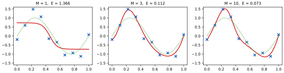
fig5_9. Download: PDF · SVG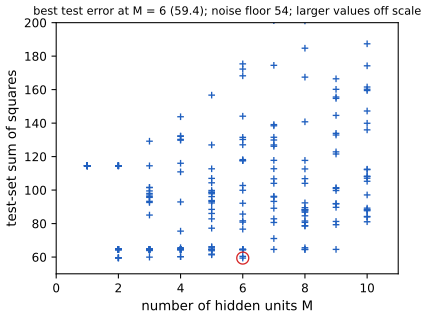
fig5_10. Download: PDF · SVG5.5.1 Consistent Gaussian priors
Result 5.12 (weight transformations and the consistent regulariser) pp. 258–259, (5.116)–(5.123); Exercise 5.24
Proof
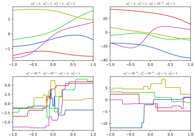
fig5_11. Download: PDF · SVG5.5.2 Early stopping
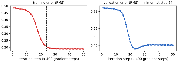
fig5_12. Download: PDF · SVGResult 5.13 (gradient descent on a quadratic is a spectral filter; early stopping and weight decay) pp. 261–262, (5.195)–(5.200); Exercise 5.25
Proof
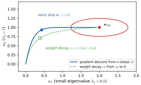
fig5_13. Download: PDF · SVG5.5.3 Invariances
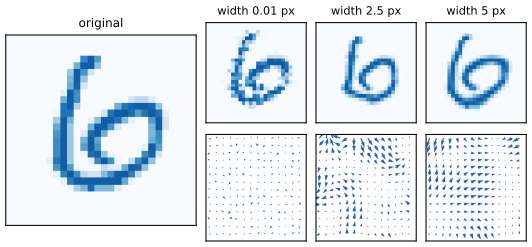
fig5_14. Download: PDF · SVG5.5.4 Tangent propagation
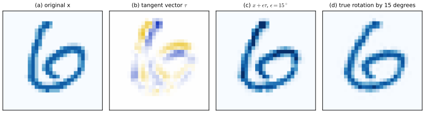
fig5_16. Download: PDF · SVGResult 5.14 (tangent propagation and its backpropagation) pp. 264–265, 288, (5.126)–(5.128), (5.201)–(5.207); Exercise 5.26
Proof (Exercise 5.26)
5.5.5 Training with transformed data
Result 5.15 (transformed data = tangent propagation to order \(\xi^2\)) pp. 266–267, (5.131)–(5.135); Exercise 5.27
Proof (including the Taylor expansion and Exercise 5.27)
5.5.6 Convolutional networks
Result 5.16 (convolutional layers: shift equivariance, parameter counts, subsampling) pp. 267–269
Proof
5.5.7 Soft weight sharing
Result 5.17 (derivatives of the soft weight-sharing regulariser) pp. 270–272, (5.141)–(5.147); Exercises 5.29–5.32
Proof
5.6 Mixture density networks
Filling the gap 5.8: why least squares returns the conditional mean, and why that fails here pp. 273, 277; Section 1.5.5
Derivation
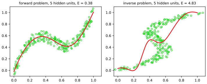
fig5_19. Download: PDF · SVGDefinition 5.2 (mixture density network) pp. 273–275, (5.148)–(5.153)
Result 5.18 (error signals of a mixture density network) p. 275, (5.154)–(5.157); Exercises 5.34–5.36
Proof
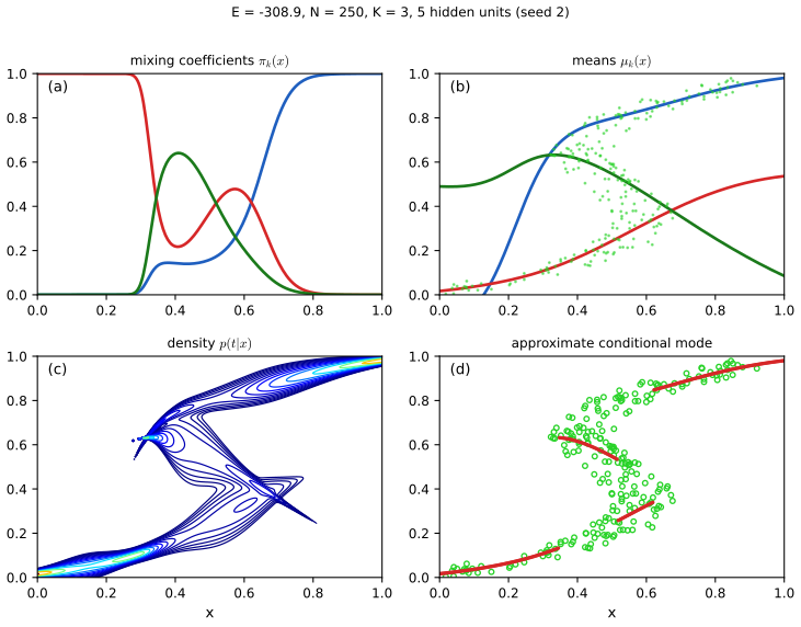
fig5_21. Download: PDF · SVGResult 5.19 (conditional mean, variance and mode) pp. 276–277, (5.158)–(5.160); Exercise 5.37
Proof
5.7 Bayesian neural networks
5.7.1 Posterior parameter distribution
Result 5.20 (Laplace posterior and predictive distribution for regression) pp. 278–280, (5.166)–(5.173); Exercise 5.38
Proof (Exercise 5.38; also the Hessian (5.166))
5.7.2 Hyperparameter optimization
Result 5.21 (evidence, re-estimation of \(\alpha\) and \(\beta\), effective number of parameters) pp. 280–281, (5.174)–(5.180); Exercise 5.39
Proof (Exercise 5.39)
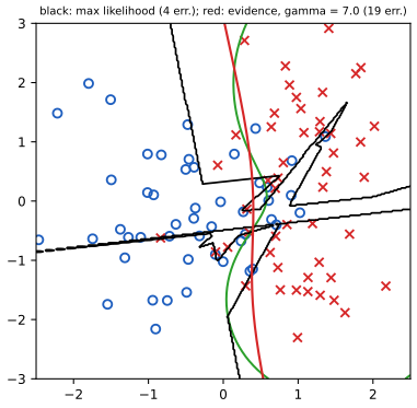
fig5_22. Download: PDF · SVG5.7.3 Bayesian neural networks for classification
Result 5.22 (evidence and predictive distribution for classification) pp. 282–284, (5.183)–(5.190); Exercises 5.40, 5.41
Proof (Exercises 5.40, 5.41, and the probit approximation)
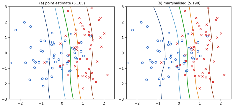
fig5_23. Download: PDF · SVGExercises
Solution
Solution
Solution
Solution
Solution
Solution
Solution
Solution
Solution
Solution
Solution
Solution
Solution
Solution
Solution
Solution
Solution
Solution
Solution
Solution
Solution
Solution
Solution
Solution
Solution
Solution
Solution
Solution
Solution
Solution
Solution
Solution
Solution
Solution
Solution
Solution
Solution
Solution
Solution
Solution
Solution
Demonstrations for this chapter
Demonstration What you can see Sections and results Two-layer network regression and backpropagation Hidden units, the network function and its hidden-unit components, a backpropagation-versus-finite-difference gradient check, weight decay and early stopping. Presets: 1 three hidden units on sin(2 pi x) (Fig. 5.3); 2 x^2, |x|, step (Fig. 5.3); 3 gradient check (5.3.2); 4 over-fitting with more hidden units (Fig. 5.9); 5 early stopping (Fig. 5.12); 6 weight decay. 5.1, 5.2, 5.3, 5.5; Result 5.1, 5.6, 5.13 Mixture density network on an inverse problem The toy inverse problem: a sum-of-squares network against a mixture density network, the mixing coefficients, means and widths, the conditional mode, and the number of components. Presets: 1 the forward problem (Fig. 5.19); 2 sum-of-squares fails on the inverse problem; 3 mixture density network (Fig. 5.21); 4 conditional mode; 5 more components. 5.6; Result 5.18, 5.19 Bayesian neural network: Laplace approximation The MAP network, posterior samples around the mode, the predictive band, the evidence over \(\alpha\) and \(\beta\) with the effective number of parameters, and Bayesian logistic-network classification. Presets: 1 MAP network; 2 posterior samples; 3 predictive band; 4 evidence over hyperparameters; 5 classification (Fig. 5.23). 5.7.1–5.7.3; Result 5.20, 5.21, 5.22 References