Model Inference and Averaging
Least squares and cross-entropy, the workhorses of the earlier chapters, are both maximum likelihood. This chapter steps back to ask how uncertain a fitted model is and how several fits can be combined. It sets three ways of answering the first question side by side on one B-spline smoother: the maximum likelihood formula, the bootstrap and the Bayesian posterior, and shows when they agree and why. It then develops the two computational tools that make likelihood and posterior computations possible when there are latent variables, the EM algorithm and Gibbs sampling, which turn out to be the "maximise" and the "sample" versions of one alternating scheme. Finally it turns the bootstrap from a way of measuring uncertainty into a way of reducing it: bagging, model averaging, stacking and bumping.
Ch. 1 Introduction Ch. 2 Supervised learning Ch. 3 Linear regression Ch. 4 Linear classification Ch. 5 Basis expansions Ch. 6 Kernel smoothing Ch. 7 Model assessment Ch. 8 Inference and averaging Ch. 9 Additive models and trees Ch. 10 Boosting Ch. 11 Neural networks Ch. 12 SVMs Ch. 13 Nearest neighbours Ch. 14 Unsupervised learning Ch. 15 Random forests Ch. 16 Ensembles Ch. 17 Graphical models Ch. 18 High-dimensional problems
How to read these notes
They follow the book. Sections carry the book's numbers (8.1, 8.2.1, ...) and every displayed equation that appears in the book carries the book's own equation number, e.g. \((8.27)\), so you can read these notes next to the book. Equations without a number are steps that the book skips.
Filling the gaps. Wherever the book says that something "can be shown", leaves it to an exercise, or states a property without proof, an orange Filling the gap box or a proof gives the full argument. Proofs and derivations start hidden: open one with its bar, or use the button below.
Figures and demonstrations. All thirteen figures of the chapter are reproduced from scratch by the Python code, plus six supplementary figures. The data of the smoothing example are not distributed with the book, so artificial data of the same kind are used; the mixture example uses the book's own Table 8.1. The ▶ Demo boxes open an interactive demonstration already set to the case being discussed.
Main reference
T. Hastie, R. Tibshirani and J. Friedman, The Elements of Statistical Learning: Data Mining, Inference, and Prediction, 2nd edition, Springer (2009), Chapter 8, pages 261–294 (book website, with the data sets: hastie.su.domains/ElemStatLearn). Section, equation, figure and exercise numbers below refer to this book. Further reading is listed in the references.
The explanations, derivations, figures and code are my own; equations are cited by their numbers in the book.
Companion courses
Much of this chapter also appears in the two companion courses on this site. The overlapping material is:
- Sections 8.2.2 and 8.3 (maximum likelihood for a linear basis model, the Gaussian posterior over the weights): Bayesian and Probabilistic Machine Learning, Section 3.1.1 and Section 3.3.1 (Result 3.11), with the unknown-variance case in Filling the gap 3.7; Foundations of Deep Learning, Section 4.1.3.
- Section 8.4 (the Dirichlet posterior): Bayesian and Probabilistic Machine Learning, Section 2.2.1 (Result 2.6).
- Section 8.5 (EM for Gaussian mixtures, the unbounded likelihood, EM in general and its lower-bound view): Bayesian and Probabilistic Machine Learning, Sections 9.2.2, 9.3 and 9.4 (Result 9.3, Results 9.14–9.15); Foundations of Deep Learning, Section 15.3 and 15.4 (Result 15.11).
- Section 8.6 (Markov chains, Gibbs sampling): Bayesian and Probabilistic Machine Learning, Sections 11.2.1 and 11.3 (Result 11.17, Result 11.20); Foundations of Deep Learning, Section 14.2.4 (Result 14.10).
- Sections 8.7–8.8 (bagging, committees, Bayesian model averaging, BIC): Bayesian and Probabilistic Machine Learning, Sections 14.1 and 14.2 (Algorithm 14.1), Result 4.19 (BIC); Foundations of Deep Learning, Section 9.6 (Result 9.11).
Where a proof there is the same, these notes state the result, sketch the argument and link to it. New here: the three-way comparison of maximum likelihood, bootstrap and Bayesian bands, the information identity and the asymptotic theory of maximum likelihood, the bootstrap as an approximate posterior, Gibbs sampling as the stochastic twin of EM, the Rao–Blackwell estimate (8.50), when bagging helps and when it hurts under 0–1 loss, stacking, bumping, and three corrections to the book (the EM estimates of the mixture example, the variance in Algorithm 8.4, a detail of Figure 8.12).
The chapter at a glance
- 8.2 For a linear smoother with Gaussian errors the parametric bootstrap reproduces the maximum likelihood band exactly (Result 8.1); in general maximum likelihood estimates are asymptotically \(\N(\theta_0,i(\theta_0)^{-1})\) (Result 8.2), because the score has mean zero and variance equal to the information (Filling the gap 8.2).
- 8.3 A Gaussian prior on the spline coefficients gives a Gaussian posterior, a ridge-type estimate (Result 8.3); as the prior variance grows it becomes the bootstrap distribution (Result 8.4).
- 8.4 The nonparametric bootstrap is close to a Bayesian posterior under a vague Dirichlet prior: same mean, covariance smaller by the factor \(N/(N+1)\) (Result 8.6).
- 8.5 EM for a two-component mixture (Algorithm 8.1); in general EM never decreases the likelihood (Result 8.8) and is coordinate ascent on a function \(F\) that equals the likelihood minus a Kullback–Leibler divergence (Result 8.9).
- 8.6 Gibbs sampling leaves the target invariant (Result 8.10); for the mixture it is EM with sampling in place of maximising, once the variance in Algorithm 8.4 is corrected (note); averaging conditional densities beats a histogram (Result 8.11).
- 8.7 Averaging over the population cannot increase squared error (Result 8.12); under 0–1 loss it helps where a classifier is right more than half of the time and hurts where it is not (Result 8.13).
- 8.8–8.9 Least squares on the fitted values of nested models puts all the weight on the largest (Result 8.14); stacking with leave-one-out predictions avoids this (Result 8.15); bumping searches model space with the bootstrap.
Notation. Training data \(\bZ=\{z_1,\dots,z_N\}\), \(z_i=(x_i,y_i)\). For the smoothing example \(h(x)^\T=(h_1(x),\dots,h_7(x))\) are cubic B-splines, \(\bH\) is the \(N\times7\) matrix with entries \(h_j(x_i)\), \(\mu(x)=h(x)^\T\beta\). For a parametric model \(g_\theta\), \(\ell(\theta)\) is the log-likelihood, \(\dot\ell\) the score, \(\mathbf I(\theta)\) the observed and \(i(\theta)\) the expected information. \(\phi_\theta\) is the normal density with \(\theta=(\mu,\sigma^2)\).
Prerequisites. Least squares and its sampling distribution (Chapter 3), B-splines (Chapter 5, Appendix), the bootstrap (Section 7.11 of the book), the multivariate Gaussian, conditional expectation and Jensen's inequality.
8.1 Introduction
p. 261 Fitting by least squares is maximum likelihood under Gaussian errors, and fitting by cross-entropy is maximum likelihood for a binomial or multinomial response. The chapter makes this general: it reviews maximum likelihood and its standard errors, sets beside it the Bayesian posterior and the bootstrap of Chapter 7, explains how the three are related, and then presents methods that combine or improve fitted models: committees, bagging, stacking and bumping.
8.2 The Bootstrap and Maximum Likelihood Methods
8.2.1 A Smoothing Example
pp. 261–264 The running example is a scatterplot smoother. The training data are \(N=50\) pairs \((x_i,y_i)\) with one input; we fit a cubic spline with three interior knots at the quartiles of the \(x_i\), a seven-dimensional space of functions written in the B-spline basis of Chapter 5, Appendix:
\[ \mu(x)=\sum_{j=1}^7\beta_jh_j(x). \tag{8.1} \]The book's 50 points are not distributed, so these notes use artificial data of the same kind: \(x_i\) uniform on \([0,3]\), \(y_i=\mu_0(x_i)+\varepsilon_i\) with a smooth curve \(\mu_0\) that has a bump, a dip and a tall peak, and \(\varepsilon_i\sim\N(0,0.55^2)\). The quartile knots are \(0.858\), \(1.542\) and \(2.260\).
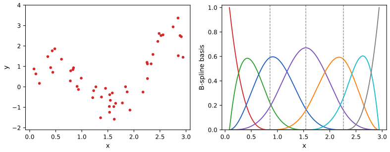
fig_8_1. Reproduces Hastie, Tibshirani and Friedman (2009), Figure 8.1. Download: PDF · SVGDefinition 8.1 (least squares fit and its standard errors) pp. 262–264, (8.2)–(8.4)
With \(\bH\) the \(N\times7\) matrix of basis values, the least squares coefficients and the estimated covariance are
\[ \hb=(\bH^\T\bH)^{-1}\bH^\T\by, \tag{8.2} \] \[ \widehat{\Var}(\hb)=(\bH^\T\bH)^{-1}\hs^2, \tag{8.3} \]where \(\hs^2=\sum_{i=1}^N(y_i-\hmu(x_i))^2/N\). The fitted curve is \(\hmu(x)=h(x)^\T\hb\), with standard error
\[ \widehat{\mathrm{se}}[\hmu(x)]=\big[h(x)^\T(\bH^\T\bH)^{-1}h(x)\big]^{1/2}\hs. \tag{8.4} \]The band \(\hmu(x)\pm1.96\,\widehat{\mathrm{se}}[\hmu(x)]\) is an approximate 95% pointwise confidence band for \(\mu(x)\).
Filling the gap 8.1: where (8.3) and (8.4) come from, and what "pointwise" means pp. 262–264
Derivation
Treat the \(x_i\) as fixed and assume \(\by=\bH\beta+\varepsilon\) with \(\E\varepsilon=0\) and \(\Cov\varepsilon=\sigma^2\bI\). Then \(\hb-\beta=(\bH^\T\bH)^{-1}\bH^\T\varepsilon\), so
\[ \Cov(\hb)=(\bH^\T\bH)^{-1}\bH^\T(\sigma^2\bI)\bH(\bH^\T\bH)^{-1}=\sigma^2(\bH^\T\bH)^{-1}. \]Replacing \(\sigma^2\) by \(\hs^2\) gives (8.3). The fitted value at \(x\) is the linear function \(h(x)^\T\hb\), so \[\Var\hmu(x)=h(x)^\T\Cov(\hb)h(x)=\sigma^2h(x)^\T(\bH^\T\bH)^{-1}h(x)\], whose estimated square root is (8.4). If the errors are Gaussian, \(\hmu(x)\sim\N(\mu(x),\Var\hmu(x))\), and \[\Pr\{|\hmu(x)-\mu(x)|\le1.96\,\mathrm{sd}\}=0.95\] because \(1.96\) is the 97.5% point of \(\N(0,1)\); with \(\hs\) in place of \(\sigma\) the level is approximate (exact intervals would use the \(t_{N-7}\) quantile and the unbiased \(\hs^2N/(N-7)\)).
The statement is about one \(x\) at a time. The probability that the whole curve lies inside the band at every \(x\) simultaneously is smaller. A simultaneous band of the same shape replaces 1.96 by \(\sqrt{\chi^2_{7}(0.95)}=3.75\) (Scheffé's method): since \(\hmu(x)-\mu(x)=h(x)^\T(\hb-\beta)\), the Cauchy–Schwarz inequality in the metric \(\bH^\T\bH\) gives
\[ \frac{\{h(x)^\T(\hb-\beta)\}^2}{h(x)^\T(\bH^\T\bH)^{-1}h(x)}\le(\hb-\beta)^\T\bH^\T\bH(\hb-\beta)\sim\sigma^2\chi^2_7 \]for every \(x\) at once. ∎
The bootstrap gives a second answer. Draw \(B\) data sets of size \(N=50\) with replacement from the pairs \(z_i\), refit the spline to each, and at every \(x\) read off the 2.5% and 97.5% points of the \(B\) fitted values; with \(B=200\) these are the fifth smallest and fifth largest. Figure 8.2 compares the two.
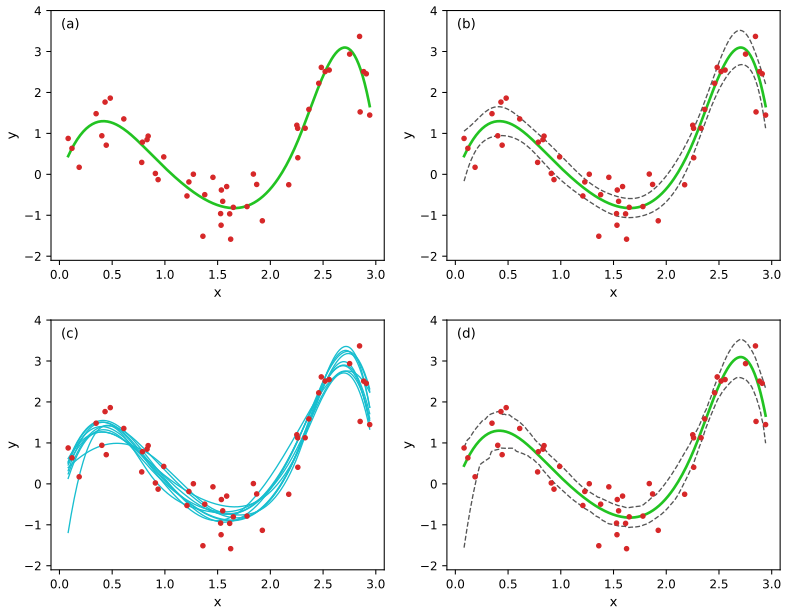
fig_8_2. Reproduces Hastie, Tibshirani and Friedman (2009), Figure 8.2. Download: PDF · SVGSuppose the errors are Gaussian:
\[ Y=\mu(X)+\varepsilon,\quad\varepsilon\sim\N(0,\sigma^2),\qquad\mu(x)=\sum_{j=1}^7\beta_jh_j(x). \tag{8.5} \]Resampling the pairs is the nonparametric bootstrap: it uses the data but no model. The parametric bootstrap instead simulates new responses from the fitted model,
\[ y_i^*=\hmu(x_i)+\varepsilon_i^*,\qquad\varepsilon_i^*\sim\N(0,\hs^2),\quad i=1,\dots,N, \tag{8.6} \]and refits the smoother to each \((x_1,y_1^*),\dots,(x_N,y_N^*)\).
Result 8.1 (the parametric bootstrap reproduces least squares) p. 264, (8.7)
Under (8.6), conditionally on the data, a bootstrap fit \(\hmu^*(x)=h(x)^\T(\bH^\T\bH)^{-1}\bH^\T\by^*\) has exactly the distribution
\[ \hmu^*(x)\sim\N\big(\hmu(x),\;h(x)^\T(\bH^\T\bH)^{-1}h(x)\,\hs^2\big). \tag{8.7} \]Hence the parametric bootstrap percentile band converges, as \(B\to\infty\), to \(\hmu(x)\pm1.96\,\widehat{\mathrm{se}}[\hmu(x)]\), the least squares band; and the average of the bootstrap fits converges to \(\hmu(x)\) itself.
Proof
Write \(\by^*=\bH\hb+\varepsilon^*\) with \(\varepsilon^*\sim\N(0,\hs^2\bI)\), independent of everything else given the data. The map \(\by^*\mapsto\hmu^*(x)=\bm l(x)^\T\by^*\), \(\bm l(x)^\T=h(x)^\T(\bH^\T\bH)^{-1}\bH^\T\), is linear, so \(\hmu^*(x)\) is Gaussian with mean \(\bm l(x)^\T\bH\hb=h(x)^\T\hb=\hmu(x)\) and variance \[\hs^2\bm l(x)^\T\bm l(x)=\hs^2h(x)^\T(\bH^\T\bH)^{-1}\bH^\T\bH(\bH^\T\bH)^{-1}h(x)=\hs^2h(x)^\T(\bH^\T\bH)^{-1}h(x)\]. The 2.5% and 97.5% points of this normal distribution are \(\hmu(x)\mp1.96\,\widehat{\mathrm{se}}\); the empirical quantiles of \(B\) independent draws converge to them almost surely (the Glivenko–Cantelli theorem, the normal distribution function being continuous and strictly increasing). By the strong law the bootstrap average converges to the mean \(\hmu(x)\). ∎
With \(B=4000\) parametric bootstrap samples the ratio of the bootstrap standard deviation to (8.4) lies between 0.988 and 1.020 at all 301 grid points, as Result 8.1 predicts.
8.2.2 Maximum Likelihood Inference
pp. 265–267 The parametric bootstrap agreed with least squares because the model has additive Gaussian errors. In general it agrees with maximum likelihood.
Definition 8.2 (likelihood, score and information) pp. 265–266, (8.8)–(8.15)
A parametric model specifies a density or mass function for the observations,
\[ z_i\sim g_\theta(z). \tag{8.8} \]For example, for a normal distribution
\[ \theta=(\mu,\sigma^2), \tag{8.9} \] \[ g_\theta(z)=\frac1{\sqrt{2\pi}\,\sigma}e^{-\frac12(z-\mu)^2/\sigma^2}. \tag{8.10} \]The likelihood and log-likelihood of independent observations are
\[ L(\theta;\bZ)=\prod_{i=1}^Ng_\theta(z_i), \tag{8.11} \] \[ \ell(\theta;\bZ)=\sum_{i=1}^N\ell(\theta;z_i)=\sum_{i=1}^N\log g_\theta(z_i), \tag{8.12} \]and the maximum likelihood estimate \(\hth\) maximises \(\ell(\theta;\bZ)\). The score is
\[ \dot\ell(\theta;\bZ)=\sum_{i=1}^N\dot\ell(\theta;z_i),\qquad\dot\ell(\theta;z_i)=\partial\ell(\theta;z_i)/\partial\theta, \tag{8.13} \]and if the maximum is attained in the interior of the parameter space, \(\dot\ell(\hth;\bZ)=0\). The information matrix is
\[ \mathbf I(\theta)=-\sum_{i=1}^N\frac{\partial^2\ell(\theta;z_i)}{\partial\theta\,\partial\theta^\T}; \tag{8.14} \]evaluated at \(\hth\) it is the observed information. The Fisher (expected) information is
\[ i(\theta)=\E_\theta[\mathbf I(\theta)]. \tag{8.15} \]Filling the gap 8.2: the score has mean zero and variance \(i(\theta)\) p. 266
Assume the support of \(g_\theta\) does not depend on \(\theta\) and that differentiation under the integral sign is allowed twice. Then for one observation, \(\E_\theta\dot\ell(\theta;z)=0\) and \[\Cov_\theta\dot\ell(\theta;z)=\E_\theta[-\partial^2\ell(\theta;z)/\partial\theta\partial\theta^\T]\]. Summing over \(N\) independent observations, \(\E_\theta\dot\ell(\theta;\bZ)=0\) and \(\Cov_\theta\dot\ell(\theta;\bZ)=i(\theta)\).
Derivation
Differentiate the identity \(\int g_\theta(z)\,\d z=1\) with respect to \(\theta\): \[0=\int\partial_\theta g_\theta\,\d z=\int(\partial_\theta\log g_\theta)\,g_\theta\,\d z=\E_\theta\dot\ell(\theta;z)\]. Differentiate once more, using \(\partial_\theta g_\theta=g_\theta\,\dot\ell\):
\[ 0=\int\Big(\frac{\partial^2\log g_\theta}{\partial\theta\partial\theta^\T}\,g_\theta+\dot\ell\,\dot\ell^\T g_\theta\Big)\d z=-\E_\theta\Big[-\frac{\partial^2\ell}{\partial\theta\partial\theta^\T}\Big]+\E_\theta[\dot\ell\dot\ell^\T]. \]Since the mean is zero, \(\E_\theta[\dot\ell\dot\ell^\T]\) is the covariance, which proves the identity. For \(N\) independent terms the means and covariances add, and \(i(\theta)=\E_\theta\mathbf I(\theta)\) is \(N\) times the one-observation information. ∎
The normal example (8.9)–(8.10). With \(\ell(\theta;z)=-\frac12\log(2\pi\sigma^2)-\frac{(z-\mu)^2}{2\sigma^2}\), the score is \(\big(\frac{z-\mu}{\sigma^2},\;-\frac1{2\sigma^2}+\frac{(z-\mu)^2}{2\sigma^4}\big)\) and
\[ -\frac{\partial^2\ell}{\partial\theta\partial\theta^\T}=\begin{pmatrix}\frac1{\sigma^2}&\frac{z-\mu}{\sigma^4}\\[2pt]\frac{z-\mu}{\sigma^4}&-\frac1{2\sigma^4}+\frac{(z-\mu)^2}{\sigma^6}\end{pmatrix},\qquad i(\theta)=N\begin{pmatrix}\frac1{\sigma^2}&0\\0&\frac1{2\sigma^4}\end{pmatrix}. \]So \(\hmu=\bar z\) has asymptotic variance \(\sigma^2/N\) (exact here) and \(\hs^2=\frac1N\sum(z_i-\bar z)^2\) has asymptotic variance \(2\sigma^4/N\); a simulation with \(N=40\) gives ratios 0.99 and 0.98 to these values.
Result 8.2 (asymptotic normality of the maximum likelihood estimate) p. 266, (8.16)–(8.19)
Let \(z_1,\dots,z_N\) be independent from \(g_{\theta_0}\), with \(\theta_0\) an interior point, the model identifiable, \(\log g_\theta\) three times differentiable in \(\theta\) with derivatives dominated by integrable functions near \(\theta_0\), and the one-observation information \(i_1(\theta_0)\) positive definite. Then a consistent root \(\hth\) of the score equation satisfies
\[ \hth\to\N\big(\theta_0,\;i(\theta_0)^{-1}\big) \tag{8.16} \]in the sense that \(\sqrt N(\hth-\theta_0)\) converges in distribution to \(\N(0,i_1(\theta_0)^{-1})\). Consequently the sampling distribution of \(\hth\) may be approximated by
\[ \N\big(\hth,\,i(\hth)^{-1}\big)\quad\text{or}\quad\N\big(\hth,\,\mathbf I(\hth)^{-1}\big), \tag{8.17} \]with standard errors
\[ \sqrt{i(\hth)^{-1}_{jj}}\quad\text{and}\quad\sqrt{\mathbf I(\hth)^{-1}_{jj}}, \tag{8.18} \]and confidence points \(\hth_j-z^{(1-\alpha)}\sqrt{i(\hth)^{-1}_{jj}}\). The likelihood ratio statistic is asymptotically chi-squared with \(p=\dim\theta\) degrees of freedom:
\[ 2[\ell(\hth)-\ell(\theta_0)]\sim\chi^2_p. \tag{8.19} \]Proof (the standard argument)
Normality. Expand the score about \(\theta_0\): \(0=\dot\ell(\hth)=\dot\ell(\theta_0)-\mathbf I(\tilde\theta)(\hth-\theta_0)\) with \(\tilde\theta\) on the segment between (row by row). Hence
\[ \sqrt N(\hth-\theta_0)=\Big[\tfrac1N\mathbf I(\tilde\theta)\Big]^{-1}\tfrac1{\sqrt N}\dot\ell(\theta_0). \]By Filling the gap 8.2, \(\frac1{\sqrt N}\dot\ell(\theta_0)\) is a normalised sum of independent terms with mean 0 and covariance \(i_1(\theta_0)\), so by the central limit theorem it converges to \(\N(0,i_1(\theta_0))\). By the law of large numbers \(\frac1N\mathbf I(\theta_0)\to i_1(\theta_0)\), and the domination of the third derivatives with consistency of \(\hth\) give \(\frac1N\mathbf I(\tilde\theta)-\frac1N\mathbf I(\theta_0)\to0\) in probability. Slutsky's theorem then gives the limit \[i_1^{-1}\N(0,i_1)=\N(0,i_1^{-1}i_1i_1^{-1})=\N(0,i_1^{-1})\]. The plug-in versions (8.17) are justified because \(i_1(\hth)\to i_1(\theta_0)\) and \(\frac1N\mathbf I(\hth)\to i_1(\theta_0)\) in probability.
Likelihood ratio. Expand \(\ell\) about \(\hth\), where the score vanishes: \[\ell(\theta_0)=\ell(\hth)-\frac12(\theta_0-\hth)^\T\mathbf I(\bar\theta)(\theta_0-\hth)\]. So \(2[\ell(\hth)-\ell(\theta_0)]=u^\T\big[\frac1N\mathbf I(\bar\theta)\big]u\) with \(u=\sqrt N(\hth-\theta_0)\to\N(0,i_1^{-1})\); a quadratic form \(u^\T i_1u\) in such a vector is \(\chi^2_p\). The resulting interval \(\{\theta_0:2[\ell(\hth)-\ell(\theta_0)]\le\chi^{2(1-2\alpha)}_p\}\) is invariant under reparametrisation and follows the shape of the likelihood, which is why the book calls it more accurate. In a simulation of the normal model with \(N=40\), the 95% region for \((\mu,\sigma^2)\) covered the truth 94.3% of the time. ∎
Back to the smoothing example: \(\theta=(\beta,\sigma^2)\) and
\[ \ell(\theta)=-\frac N2\log\sigma^22\pi-\frac1{2\sigma^2}\sum_{i=1}^N\big(y_i-h(x_i)^\T\beta\big)^2. \tag{8.20} \]Filling the gap 8.3: maximum likelihood and the information for the smoothing model p. 267, (8.21)–(8.22)
Setting \(\partial\ell/\partial\beta=0\) and \(\partial\ell/\partial\sigma^2=0\) gives
\[ \hb=(\bH^\T\bH)^{-1}\bH^\T\by,\qquad\hs^2=\frac1N\sum\big(y_i-\hmu(x_i)\big)^2, \tag{8.21} \]the estimates (8.2) and (8.3). The information for \((\beta,\sigma^2)\) is block diagonal, with \(\beta\) block
\[ \mathbf I(\beta)=(\bH^\T\bH)/\sigma^2, \tag{8.22} \]so \(\mathbf I(\beta)^{-1}\) evaluated at \(\hs^2\) is the least squares covariance (8.3).
Derivation
Write \(r(\beta)=\by-\bH\beta\). Then \(\partial\ell/\partial\beta=\bH^\T r(\beta)/\sigma^2\), which vanishes exactly at the normal equations \(\bH^\T\bH\beta=\bH^\T\by\), whatever \(\sigma^2\) is; and \(\partial\ell/\partial\sigma^2=-\frac N{2\sigma^2}+\frac{\|r\|^2}{2\sigma^4}\), which vanishes at \(\sigma^2=\|r(\hb)\|^2/N\). The profile \(\ell(\hb,\sigma^2)\) is \(-\frac N2\log\sigma^2-\frac{\|r\|^2}{2\sigma^2}+\)const, maximised there, so this is the maximum. The second derivatives are
\[ \frac{\partial^2\ell}{\partial\beta\partial\beta^\T}=-\frac{\bH^\T\bH}{\sigma^2},\qquad\frac{\partial^2\ell}{\partial\beta\,\partial\sigma^2}=-\frac{\bH^\T r(\beta)}{\sigma^4},\qquad\frac{\partial^2\ell}{\partial(\sigma^2)^2}=\frac N{2\sigma^4}-\frac{\|r\|^2}{\sigma^6}. \]The cross term is zero at \(\hb\) (observed information) and has expectation zero at the true \(\beta\) (expected information), because \(\E r=0\); this is the block diagonality. The \(\sigma^2\) entry is \(N/(2\hs^4)\) at the maximum and \(N/(2\sigma^4)\) in expectation. A numerical Hessian of (8.20) at the fitted values confirms all three blocks. ∎
See also (companion courses): Result 3.1 and Result 3.2 of Bayesian and Probabilistic Machine Learning (maximum likelihood for a linear basis model); Foundations of Deep Learning, Section 4.1.3.
8.2.3 Bootstrap versus Maximum Likelihood
p. 267 The bootstrap is a computer implementation of nonparametric or parametric maximum likelihood. Its advantage is that it needs no formula: it gives standard errors and bands for any procedure we can rerun. Suppose, for example, that the number of knots is chosen from the data. No formula accounts for that choice; the bootstrap does, by making the choice again in every bootstrap sample.
On our data, leave-one-out cross-validation (computed from one fit through the hat matrix, choose_K_loocv) over \(K=1,\dots,8\) quantile knots picks \(K=3\), the fixed choice used above. Repeating the choice in each of the 200 bootstrap samples of Figure 8.2, the samples pick every value from 1 to 8 knots (counts 8, 46, 38, 17, 20, 33, 22, 16 for \(K=1,\dots,8\)), and the average width of the 95% band grows from 0.711 to 1.098. The book reports that for its data the adaptive bands did not look much different from the fixed ones; for these data the knot choice is far from stable, and accounting for it widens the band by half. Which happens depends on how sharply the cross-validation curve is minimised.
8.3 Bayesian Methods
pp. 267–270 A Bayesian analysis specifies a sampling model \(\Pr(\bZ\given\theta)\) and a prior \(\Pr(\theta)\), and computes the posterior
\[ \Pr(\theta\given\bZ)=\frac{\Pr(\bZ\given\theta)\cdot\Pr(\theta)}{\int\Pr(\bZ\given\theta)\cdot\Pr(\theta)\,\d\theta}, \tag{8.23} \]which describes what is known about \(\theta\) after the data. Future data are predicted by the predictive distribution
\[ \Pr(z^{\mathrm{new}}\given\bZ)=\int\Pr(z^{\mathrm{new}}\given\theta)\cdot\Pr(\theta\given\bZ)\,\d\theta, \tag{8.24} \]which, unlike the plug-in \(\Pr(z^{\mathrm{new}}\given\hth)\), accounts for the uncertainty about \(\theta\).
For the smoothing example take model (8.5) with \(\sigma^2\) known and the \(x_i\) fixed, and put a Gaussian prior on the coefficients,
\[ \beta\sim\N(0,\tau\Sigma). \tag{8.25} \]This implies a Gaussian process prior for the curve, with covariance kernel
\[ K(x,x')=\Cov[\mu(x),\mu(x')]=\tau\cdot h(x)^\T\Sigma h(x'), \tag{8.26} \]since \(\mu(x)=h(x)^\T\beta\) is linear in \(\beta\). The book takes \(\Sigma=\bI\): smoothness is already built into the low-dimensional B-spline basis.
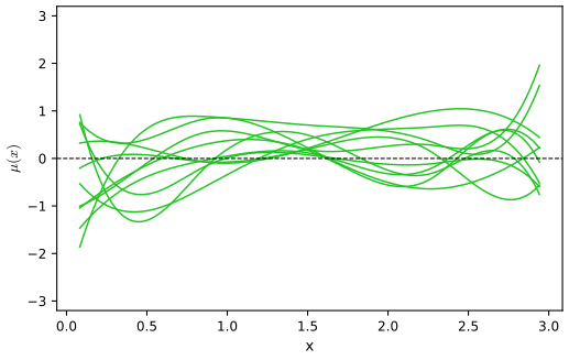
fig_8_3. Reproduces Hastie, Tibshirani and Friedman (2009), Figure 8.3. Download: PDF · SVGResult 8.3 (the posterior for the spline coefficients) p. 269, (8.27)–(8.28)
Under (8.5) with known \(\sigma^2\) and the prior (8.25), the posterior of \(\beta\) is Gaussian with
\[ \E(\beta\given\bZ)=\Big(\bH^\T\bH+\frac{\sigma^2}\tau\Sigma^{-1}\Big)^{-1}\bH^\T\by,\qquad\Cov(\beta\given\bZ)=\Big(\bH^\T\bH+\frac{\sigma^2}\tau\Sigma^{-1}\Big)^{-1}\sigma^2, \tag{8.27} \]and correspondingly
\[ \E(\mu(x)\given\bZ)=h(x)^\T\Big(\bH^\T\bH+\frac{\sigma^2}\tau\Sigma^{-1}\Big)^{-1}\bH^\T\by,\qquad\Cov[\mu(x),\mu(x')\given\bZ]=h(x)^\T\Big(\bH^\T\bH+\frac{\sigma^2}\tau\Sigma^{-1}\Big)^{-1}h(x')\,\sigma^2. \tag{8.28} \]The posterior mean is a generalised ridge regression estimate with penalty \(\frac{\sigma^2}{\tau}\beta^\T\Sigma^{-1}\beta\).
Filling the gap 8.4: completing the square p. 269
Derivation
Up to terms that do not involve \(\beta\), the log posterior is the log-likelihood plus the log prior:
\[ \log\Pr(\beta\given\bZ)=-\frac1{2\sigma^2}\|\by-\bH\beta\|^2-\frac1{2\tau}\beta^\T\Sigma^{-1}\beta+c=-\frac1{2\sigma^2}\Big[\beta^\T\bA\beta-2\beta^\T\bH^\T\by\Big]+c', \]with \(\bA=\bH^\T\bH+\frac{\sigma^2}\tau\Sigma^{-1}\), positive definite. Completing the square, \[\beta^\T\bA\beta-2\beta^\T\bH^\T\by=(\beta-\bA^{-1}\bH^\T\by)^\T\bA(\beta-\bA^{-1}\bH^\T\by)-\by^\T\bH\bA^{-1}\bH^\T\by\]. A density proportional to \(\exp\{-\frac12(\beta-m)^\T(\sigma^{-2}\bA)(\beta-m)\}\) is \(\N(m,\sigma^2\bA^{-1})\), which is (8.27). Since \(\mu(x)=h(x)^\T\beta\) is a linear function of a Gaussian vector, its posterior mean and covariance are obtained by applying \(h(x)^\T\) on the left and \(h(x')\) on the right: (8.28). The posterior mode maximises the same quadratic, which is the penalised least squares criterion \(\|\by-\bH\beta\|^2+\frac{\sigma^2}\tau\beta^\T\Sigma^{-1}\beta\). The same posterior is obtained, as a check, from the joint Gaussian distribution of \((\beta,\by)\) and the conditioning formula \[\E(\beta\given\by)=\tau\Sigma\bH^\T(\tau\bH\Sigma\bH^\T+\sigma^2\bI)^{-1}\by\]; the two agree by the matrix inversion lemma (confirmed numerically for \(\tau=1\) and 37). ∎
See also (companion course): Result 3.11 of Bayesian and Probabilistic Machine Learning, the same posterior with \(\Sigma=\bI\) in precision notation (\(\alpha=1/\tau\), \(\beta_{\mathrm{noise}}=1/\sigma^2\)), and the Bayesian regression demo.
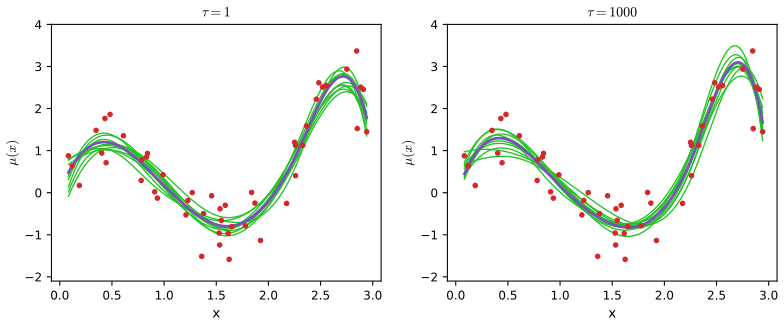
fig_8_4. Reproduces Hastie, Tibshirani and Friedman (2009), Figure 8.4. Download: PDF · SVGResult 8.4 (a flat prior gives the bootstrap distribution) p. 270
As \(\tau\to\infty\), the posterior (8.27) converges to \(\N\big(\hb,(\bH^\T\bH)^{-1}\sigma^2\big)\), and the posterior of \(\mu(x)\) to \(\N\big(\hmu(x),h(x)^\T(\bH^\T\bH)^{-1}h(x)\sigma^2\big)\). With \(\sigma^2=\hs^2\) this is exactly the parametric bootstrap distribution (8.7).
Proof
\(\bA_\tau=\bH^\T\bH+\frac{\sigma^2}\tau\Sigma^{-1}\to\bH^\T\bH\), which is invertible (seven distinct B-splines evaluated at 50 distinct points span a seven-dimensional space), and matrix inversion is continuous at invertible matrices, so \(\bA_\tau^{-1}\to(\bH^\T\bH)^{-1}\). The mean and covariance of (8.27) converge, and Gaussian distributions converge when their means and covariances do. Compare with (8.7). ∎
The limit \(\tau\to\infty\) is a noninformative (flat) prior. In Gaussian models, maximum likelihood, the parametric bootstrap and the Bayesian analysis with a flat prior agree, because with a constant prior the posterior is proportional to the likelihood. With \(\tau=1\) the posterior is not the bootstrap: the prior is an extra source of information that shrinks and smooths.
Filling the gap 8.5: doing it properly, with a prior on \(\sigma\) p. 270
The analysis above used \(\hs^2\) in place of \(\sigma^2\). With the flat prior on \(\beta\) and the standard prior \(g(\sigma)\propto1/\sigma\) (equivalently \(\Pr(\sigma^2)\propto1/\sigma^2\)), the marginal posterior of \(\beta\), with \(\sigma\) integrated out, is a multivariate \(t\) distribution:
\[ \beta\given\bZ\sim t_{N-p}\Big(\hb,\;\frac{\mathrm{RSS}}{N-p}(\bH^\T\bH)^{-1}\Big),\qquad p=7, \]so that \(\mu(x)\) has a posterior \(t_{N-p}\) distribution centred at \(\hmu(x)\) with scale \(\big[h(x)^\T(\bH^\T\bH)^{-1}h(x)\big]^{1/2}s\), \(s^2=\mathrm{RSS}/(N-p)\). The 95% posterior interval is then exactly the classical \(t\) confidence interval.
Derivation
With \(\mathrm{RSS}=\|\by-\bH\hb\|^2\), the identity \[\|\by-\bH\beta\|^2=\mathrm{RSS}+(\beta-\hb)^\T\bH^\T\bH(\beta-\hb)=:\mathrm{RSS}+Q(\beta)\] gives the joint posterior
\[ \Pr(\beta,\sigma^2\given\bZ)\propto(\sigma^2)^{-N/2-1}\exp\Big\{-\frac{\mathrm{RSS}+Q(\beta)}{2\sigma^2}\Big\}. \]Integrating out \(\sigma^2\) with \(\int_0^\infty v^{-a-1}e^{-b/v}\d v=\Gamma(a)b^{-a}\), \(a=N/2\), gives \[\Pr(\beta\given\bZ)\propto\{\mathrm{RSS}+Q(\beta)\}^{-N/2}\propto\{1+\frac{Q(\beta)}{(N-p)s^2}\}^{-(N-p+p)/2}\], the multivariate \(t\) density with \(N-p\) degrees of freedom, location \(\hb\) and scale matrix \(s^2(\bH^\T\bH)^{-1}\). A linear function \(h(x)^\T\beta\) of a multivariate \(t\) vector is univariate \(t\) with the same degrees of freedom and the projected scale. For \(N=50\), \(p=7\), the 97.5% point of \(t_{43}\) is 2.017 against 1.96, and \(s^2=\hs^2\cdot50/43\): the honest Bayesian band is about 10% wider than the plug-in one. The companion course derives the same \(t\) form in precision notation in Filling the gap 3.7. ∎
8.4 Relationship Between the Bootstrap and Bayesian Inference
pp. 271–272 Start with a single observation from a normal distribution,
\[ z\sim\N(\theta,1), \tag{8.29} \]and the prior \(\theta\sim\N(0,\tau)\).
Result 8.5 (the normal example) p. 271, (8.30)–(8.31)
\[ \theta\given z\sim\N\Big(\frac z{1+1/\tau},\;\frac1{1+1/\tau}\Big), \tag{8.30} \]and as \(\tau\to\infty\),
\[ \theta\given z\sim\N(z,1), \tag{8.31} \]which is the parametric bootstrap distribution of \(z^*\sim\N(\hth,1)\), \(\hth=z\).
Proof
\[\log\Pr(\theta\given z)=-\frac12(z-\theta)^2-\frac{\theta^2}{2\tau}+c=-\frac12(1+\frac1\tau)\theta^2+z\theta+c'\]. A quadratic \(-\frac12a\theta^2+b\theta\) in the exponent is a \(\N(b/a,1/a)\) density, here with \(a=1+1/\tau\), \(b=z\). Let \(\tau\to\infty\). (Checked by numerical integration for \(\tau=0.5\) and 4.) ∎
Three things make the correspondence work: (1) a noninformative prior; (2) the log-likelihood depends on the data only through \(\hth\), \(\ell(\theta;\bZ)=\ell(\theta;\hth)\); and (3) it is symmetric in \(\theta\) and \(\hth\), \(\ell(\theta;\hth)=\ell(\hth;\theta)+\)const. Then the posterior \(\propto\exp\ell(\theta;\hth)\), as a function of \(\theta\), has the same shape as the sampling density of \(\hth^*\) around \(\hth\). Properties (2) and (3) hold essentially only for the Gaussian, but approximately for the multinomial, which is the model behind the nonparametric bootstrap.
Let the sample space have \(L\) categories with probabilities \(w=(w_1,\dots,w_L)\), observed proportions \(\hat w\), and estimator \(S(\hat w)\). Take the symmetric Dirichlet prior
\[ w\sim\Di_L(a\mathbf 1), \tag{8.32} \]with density proportional to \(\prod_\ell w_\ell^{a-1}\).
Result 8.6 (the bootstrap as an approximate noninformative posterior) p. 272, (8.33)–(8.35)
The posterior is
\[ w\sim\Di_L(a\mathbf 1+N\hat w), \tag{8.33} \]and in the noninformative limit \(a\to0\),
\[ w\sim\Di_L(N\hat w). \tag{8.34} \]The bootstrap distribution of the resampled proportions is
\[ N\hat w^*\sim\Mult(N,\hat w). \tag{8.35} \]Both have mean \(\hat w\) and support on the categories with \(\hat w_\ell>0\); their covariances are
\[ \Cov(w\given\bZ)=\frac{\diag(\hat w)-\hat w\hat w^\T}{N+1},\qquad\Cov(\hat w^*)=\frac{\diag(\hat w)-\hat w\hat w^\T}N. \]So the bootstrap distribution of \(S(\hat w^*)\) approximates the posterior of \(S(w)\), with variances that differ by the factor \(N/(N+1)\) for linear statistics.
Proof
The likelihood of \(N\) independent draws with counts \(N\hat w_\ell\) is \(\prod_\ell w_\ell^{N\hat w_\ell}\); multiplied by the prior \(\prod_\ell w_\ell^{a-1}\) it gives \(\prod_\ell w_\ell^{a+N\hat w_\ell-1}\) on the simplex, the \(\Di_L(a\mathbf1+N\hat w)\) kernel (8.33). Letting \(a\to0\) gives (8.34) on the face of the simplex where \(\hat w_\ell>0\) (a Dirichlet parameter of 0 puts the component at 0). For \(\alpha=N\hat w\), with \(\alpha_0=\sum\alpha_\ell=N\), the Dirichlet moments (Result 2.6 of the companion course) are \(\E w_\ell=\alpha_\ell/\alpha_0=\hat w_\ell\) and
\[ \Cov(w_\ell,w_m)=\frac{\alpha_\ell(\alpha_0\delta_{\ell m}-\alpha_m)}{\alpha_0^2(\alpha_0+1)}=\frac{\hat w_\ell\delta_{\ell m}-\hat w_\ell\hat w_m}{N+1}. \]For the multinomial, \(\E N\hat w^*_\ell=N\hat w_\ell\), \(\Var(N\hat w^*_\ell)=N\hat w_\ell(1-\hat w_\ell)\) and \(\Cov(N\hat w^*_\ell,N\hat w^*_m)=-N\hat w_\ell\hat w_m\); dividing by \(N^2\) gives the second formula. For a linear statistic \(S(w)=\sum_\ell w_\ell s_\ell\) the two variances are \(v/(N+1)\) and \(v/N\), \(v=\sum\hat w_\ell s_\ell^2-(\sum\hat w_\ell s_\ell)^2\). ∎
With the data as categories (each \(z_i\) its own category, \(\hat w_\ell=1/N\)), (8.34) is \(\Di_N(1,\dots,1)\): the posterior gives the data points uniform-on-the-simplex random weights. This is Rubin's (1981) Bayesian bootstrap; the ordinary bootstrap gives them multinomial weights instead.
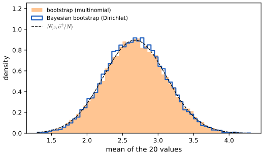
fig_8_s1. Download: PDF · SVGIn this sense the bootstrap distribution is an approximate nonparametric, noninformative posterior, obtained "painlessly": no prior has to be written down and no posterior has to be sampled. By perturbing the data the bootstrap imitates the Bayesian perturbation of the parameters.
See also (companion course): the Dirichlet distribution and its conjugacy in Bayesian and Probabilistic Machine Learning, Section 2.2.1.
8.5 The EM Algorithm
p. 272 The EM algorithm simplifies difficult maximum likelihood problems by adding latent data that, if they were observed, would make the problem easy. It is introduced on a simple mixture model.
8.5.1 Two-Component Mixture Model
pp. 272–275 Table 8.1 of the book lists twenty fictitious values; their histogram (Figure 8.5, left) has two humps, so one Gaussian will not do. Model \(Y\) as a mixture of two normals:
\[ Y_1\sim\N(\mu_1,\sigma_1^2),\qquad Y_2\sim\N(\mu_2,\sigma_2^2),\qquad Y=(1-\Delta)\cdot Y_1+\Delta\cdot Y_2, \tag{8.36} \]with \(\Delta\in\{0,1\}\), \(\Pr(\Delta=1)=\pi\). The density of \(Y\) is
\[ g_Y(y)=(1-\pi)\phi_{\theta_1}(y)+\pi\phi_{\theta_2}(y), \tag{8.37} \]with parameters
\[ \theta=(\pi,\theta_1,\theta_2)=(\pi,\mu_1,\sigma_1^2,\mu_2,\sigma_2^2), \tag{8.38} \]and log-likelihood
\[ \ell(\theta;\bZ)=\sum_{i=1}^N\log\big[(1-\pi)\phi_{\theta_1}(y_i)+\pi\phi_{\theta_2}(y_i)\big]. \tag{8.39} \]The sum inside the logarithm makes direct maximisation awkward. If the labels \(\Delta_i\) were known, the log-likelihood would be
\[ \ell_0(\theta;\bZ,\Delta)=\sum_{i=1}^N\big[(1-\Delta_i)\log\phi_{\theta_1}(y_i)+\Delta_i\log\phi_{\theta_2}(y_i)\big]+\sum_{i=1}^N\big[(1-\Delta_i)\log(1-\pi)+\Delta_i\log\pi\big], \tag{8.40} \]which separates: \(\mu_1,\sigma_1^2\) would be the mean and variance of the points with \(\Delta_i=0\), \(\mu_2,\sigma_2^2\) those of the points with \(\Delta_i=1\), and \(\pi\) the proportion of ones. EM replaces each unknown \(\Delta_i\) by its expected value, the responsibility of component 2 for observation \(i\),
\[ \gamma_i(\theta)=\E(\Delta_i\given\theta,\bZ)=\Pr(\Delta_i=1\given\theta,\bZ). \tag{8.41} \]Algorithm 8.1 (EM for a two-component Gaussian mixture) p. 275
- Start from initial guesses \(\hmu_1,\hs_1^2,\hmu_2,\hs_2^2,\hat\pi\).
- Expectation step: compute the responsibilities \[ \hat\gamma_i=\frac{\hat\pi\phi_{\hth_2}(y_i)}{(1-\hat\pi)\phi_{\hth_1}(y_i)+\hat\pi\phi_{\hth_2}(y_i)},\qquad i=1,2,\dots,N. \tag{8.42} \]
- Maximisation step: compute the weighted means and variances \[ \hmu_1=\frac{\sum_{i=1}^N(1-\hat\gamma_i)y_i}{\sum_{i=1}^N(1-\hat\gamma_i)},\quad\hs_1^2=\frac{\sum_{i=1}^N(1-\hat\gamma_i)(y_i-\hmu_1)^2}{\sum_{i=1}^N(1-\hat\gamma_i)},\quad\hmu_2=\frac{\sum_{i=1}^N\hat\gamma_iy_i}{\sum_{i=1}^N\hat\gamma_i},\quad\hs_2^2=\frac{\sum_{i=1}^N\hat\gamma_i(y_i-\hmu_2)^2}{\sum_{i=1}^N\hat\gamma_i}, \] and the mixing probability \(\hat\pi=\sum_{i=1}^N\hat\gamma_i/N\).
- Iterate steps 2 and 3 until convergence.
Filling the gap 8.6: why these are the E and M steps pp. 274–275
Derivation
E step. The pairs \((y_i,\Delta_i)\) are independent, so \(\Delta_i\) given all the data depends only on \(y_i\). By Bayes' rule with the joint density \(\Pr(\Delta_i=1,y_i)=\pi\phi_{\theta_2}(y_i)\) and \(\Pr(\Delta_i=0,y_i)=(1-\pi)\phi_{\theta_1}(y_i)\),
\[ \Pr(\Delta_i=1\given y_i,\theta)=\frac{\pi\phi_{\theta_2}(y_i)}{(1-\pi)\phi_{\theta_1}(y_i)+\pi\phi_{\theta_2}(y_i)}, \]which is (8.42). Because (8.40) is linear in the \(\Delta_i\), its conditional expectation is (8.40) with \(\Delta_i\) replaced by \(\gamma_i\):
\[ Q(\theta',\theta)=\sum_i\Big[(1-\gamma_i)\log\phi_{\theta_1'}(y_i)+\gamma_i\log\phi_{\theta_2'}(y_i)+(1-\gamma_i)\log(1-\pi')+\gamma_i\log\pi'\Big]. \]M step. \(Q\) separates into a part in \(\pi'\), a part in \(\theta_1'\) and a part in \(\theta_2'\). For \(\pi'\): \(\frac{\d}{\d\pi'}=-\frac{\sum(1-\gamma_i)}{1-\pi'}+\frac{\sum\gamma_i}{\pi'}=0\) gives \(\pi'=\sum\gamma_i/N\), and the function is concave. For \(\theta_2'=(\mu,v)\): \(\sum_i\gamma_i[-\frac12\log(2\pi v)-\frac{(y_i-\mu)^2}{2v}]\) has \(\partial_\mu=\sum\gamma_i(y_i-\mu)/v=0\), so \(\mu=\sum\gamma_iy_i/\sum\gamma_i\), and \(\partial_v=-\frac{\sum\gamma_i}{2v}+\frac{\sum\gamma_i(y_i-\mu)^2}{2v^2}=0\), so \(v=\sum\gamma_i(y_i-\mu)^2/\sum\gamma_i\): the weighted mean and variance. This is the unique maximum (the same argument as for one Gaussian, with weights). Component 1 is the same with weights \(1-\gamma_i\). ∎
See also (companion courses): the \(K\)-component, multivariate version in Bayesian and Probabilistic Machine Learning, Section 9.2.2 (Algorithm 9.3) and Foundations of Deep Learning, Section 15.3.1.
The book's starting values: two of the \(y_i\) chosen at random for \(\hmu_1,\hmu_2\), the overall sample variance \(\sum(y_i-\bar y)^2/N\) for both variances, and \(\hat\pi=0.5\).
Result 8.7 (the mixture likelihood is unbounded) p. 274
Put \(\mu_1=y_j\) for some \(j\) and fix the other parameters with \(0\lt\pi\lt1\), \(\sigma_2^2>0\). Then \(\ell(\theta)\to+\infty\) as \(\sigma_1^2\to0\). The maximum likelihood estimate in the strict sense does not exist; one looks for a good local maximum with both variances positive.
Proof
The \(j\)-th term of (8.39) is at least \[\log\{(1-\pi)\phi_{\theta_1}(y_j)\}=\log(1-\pi)-\frac12\log(2\pi\sigma_1^2)\to\infty\], while every other term is at least \(\log\{\pi\phi_{\theta_2}(y_i)\}\), a finite constant. In the code, decreasing \(\sigma_1^2\) by a factor 100 adds \(\log 10=2.30\) to \(\ell\), as the formula says. The companion course gives the multivariate version: Result 9.3. ∎
Running EM to convergence from all 380 ordered pairs of data points as starting means (both variances stay above 0.6 along every path, so no run approaches a spike) gives one and the same maximum,
\[ \hmu_1=4.656,\quad\hs_1^2=0.819,\quad\hmu_2=1.083,\quad\hs_2^2=0.811,\quad\hat\pi=0.555,\qquad\ell=-38.913. \]The speed differs a lot between starts: after 25 iterations some runs are still on a plateau with log-likelihood near \(-42.2\), where the two components almost coincide, before they climb. (Component 2, with \(\hat\pi=0.555\), is the left one, as in the book.)
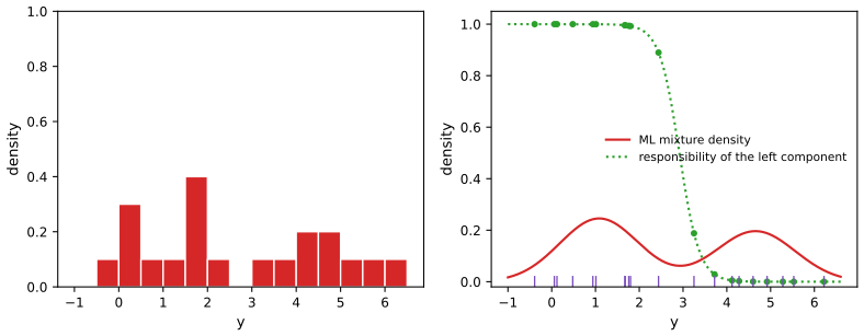
fig_8_5. Reproduces Hastie, Tibshirani and Friedman (2009), Figure 8.5. Download: PDF · SVGTable 8.2, recomputed: \(\hat\pi\) at selected EM iterations p. 275
Started from \(\hmu_1=y_7=3.72\), \(\hmu_2=y_4=1.67\) (the pair whose path is closest to the book's table):
| iteration | 1 | 5 | 10 | 15 | 20 | converged |
|---|---|---|---|---|---|---|
| \(\hat\pi\), here | 0.505 | 0.493 | 0.521 | 0.550 | 0.554 | 0.5546 |
| \(\hat\pi\), book | 0.485 | 0.493 | 0.523 | 0.544 | 0.546 | 0.546 |
Note on the book: the reported estimates are not yet converged p. 275
The book gives the final estimates \(\hmu_1=4.62\), \(\hs_1^2=0.87\), \(\hmu_2=1.06\), \(\hs_2^2=0.77\), \(\hat\pi=0.546\). These are not a fixed point of EM: one more iteration from them moves \(\hat\pi\) to 0.549, \(\hmu_1\) to 4.634 and \(\hs_1^2\) to 0.853, and their log-likelihood, \(-38.924\), is below the maximum \(-38.913\) reached at \((4.656,0.819,1.083,0.811,0.555)\). They look like the values after the twentieth iteration of a run that had not finished, which is consistent with Table 8.2 still changing between iterations 15 and 20. The difference is small, but the converged values are the maximum likelihood estimates, and they are the ones used for Figures 8.5 and 8.8 here.
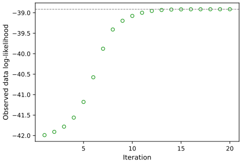
fig_8_6. Reproduces Hastie, Tibshirani and Friedman (2009), Figure 8.6. Download: PDF · SVG8.5.2 The EM Algorithm in General
pp. 276–277 EM (also called Baum–Welch in hidden Markov models) applies when the likelihood is hard to maximise but would become easy if the sample were enlarged by latent data, an idea called data augmentation. Let \(\bZ\) be the observed data with log-likelihood \(\ell(\theta;\bZ)\), \(\bZ^m\) the latent or missing data, and \(\bT=(\bZ,\bZ^m)\) the complete data with log-likelihood \(\ell_0(\theta;\bT)\). For the mixture, \((\bZ,\bZ^m)=(\by,\Delta)\) and \(\ell_0\) is (8.40).
Algorithm 8.2 (the EM algorithm) p. 277
- Start with initial guesses \(\hth^{(0)}\).
- Expectation step: at the \(j\)-th step compute, as a function of the dummy argument \(\theta'\), \[ Q(\theta',\hth^{(j)})=\E\big(\ell_0(\theta';\bT)\given\bZ,\hth^{(j)}\big). \tag{8.43} \]
- Maximisation step: let \(\hth^{(j+1)}\) be the maximiser of \(Q(\theta',\hth^{(j)})\) over \(\theta'\).
- Iterate steps 2 and 3 until convergence.
For the mixture, \(Q\) is (8.40) with \(\Delta_i\) replaced by \(\hat\gamma_i\) (Filling the gap 8.6). Why does maximising \(Q\) rather than \(\ell\) increase \(\ell\)? Since
\[ \Pr(\bZ^m\given\bZ,\theta')=\frac{\Pr(\bZ^m,\bZ\given\theta')}{\Pr(\bZ\given\theta')}, \tag{8.44} \] \[ \Pr(\bZ\given\theta')=\frac{\Pr(\bT\given\theta')}{\Pr(\bZ^m\given\bZ,\theta')}. \tag{8.45} \]Taking logarithms, \(\ell(\theta';\bZ)=\ell_0(\theta';\bT)-\ell_1(\theta';\bZ^m\given\bZ)\), where \(\ell_1\) is the log of the conditional density of the latent data. The left side does not involve \(\bZ^m\), so taking the expectation over \(\bZ^m\) with respect to \(\Pr(\bZ^m\given\bZ,\theta)\) changes nothing:
\[ \ell(\theta';\bZ)=\E[\ell_0(\theta';\bT)\given\bZ,\theta]-\E[\ell_1(\theta';\bZ^m\given\bZ)\given\bZ,\theta]\equiv Q(\theta',\theta)-R(\theta',\theta). \tag{8.46} \]Result 8.8 (EM never decreases the likelihood) p. 277, (8.47); Exercise 8.1
For all \(\theta'\), \(R(\theta',\theta)\le R(\theta,\theta)\). Hence if \(Q(\theta',\theta)\ge Q(\theta,\theta)\), in particular if \(\theta'\) maximises \(Q(\cdot,\theta)\),
\[ \ell(\theta';\bZ)-\ell(\theta;\bZ)=[Q(\theta',\theta)-Q(\theta,\theta)]-[R(\theta',\theta)-R(\theta,\theta)]\ge0. \tag{8.47} \]So any step that increases \(Q\) (a generalised EM or GEM step) is enough.
Proof
Write \(p=\Pr(\bZ^m\given\bZ,\theta)\) and \(q=\Pr(\bZ^m\given\bZ,\theta')\), two densities in \(\bZ^m\). Then \(R(\theta',\theta)-R(\theta,\theta)=\E_p[\log(q/p)]\). The logarithm is concave, so by Jensen's inequality \[\E_p\log(q/p)\le\log\E_p(q/p)=\log\int q=\log1=0\] (the integral is over the support of \(p\), so it is at most 1, which only helps). Equality holds iff \(q=p\) almost everywhere. This is Exercise 8.1 with \(r=q\); the gap \(R(\theta,\theta)-R(\theta',\theta)\) is the Kullback–Leibler divergence \(\KL(p\,\|\,q)\ge0\). Then (8.47) is (8.46) at \(\theta'\) minus (8.46) at \(\theta\). Numerically: along all 380 EM runs of the mixture example, the log-likelihood never decreases, and (8.46) and the inequality hold to machine precision for 200 random pairs \((\theta',\theta)\). ∎
Two cautions that the monotonicity does not remove. A nondecreasing bounded sequence of likelihood values converges, but the parameters converge only to a stationary point (Wu, 1983): a local maximum or, as with the symmetric start of the demonstration, a saddle. And near the maximum EM is linearly convergent, with rate governed by the fraction of the information that is missing, so it can be slow when the components overlap. The EM algorithm can also be seen as a minorisation (MM) algorithm (Exercise 8.7).
See also (companion courses): Bayesian and Probabilistic Machine Learning, Section 9.4 (Result 9.14, the decomposition, and Result 9.15) and Foundations of Deep Learning, Section 15.4.1.
8.5.3 EM as a Maximization–Maximization Procedure
pp. 277–279 For any distribution \(\tP(\bZ^m)\) over the latent data define
\[ F(\theta',\tP)=\E_{\tP}[\ell_0(\theta';\bT)]-\E_{\tP}[\log\tP(\bZ^m)]. \tag{8.48} \]In the mixture, \(\tP\) is a set of probabilities \(\gamma_i=\Pr(\Delta_i=1)\), one per observation, and the second term is the entropy \[-\sum_i[\gamma_i\log\gamma_i+(1-\gamma_i)\log(1-\gamma_i)]\].
Result 8.9 (EM is coordinate ascent on \(F\)) p. 278, (8.49); Exercise 8.2
For every \(\theta'\) and \(\tP\),
\[ F(\theta',\tP)=\ell(\theta';\bZ)-\KL\big(\tP\,\big\|\,\Pr(\bZ^m\given\bZ,\theta')\big)\le\ell(\theta';\bZ). \]Hence, for fixed \(\theta'\), \(F\) is maximised over \(\tP\) by
\[ \tP(\bZ^m)=\Pr(\bZ^m\given\bZ,\theta'), \tag{8.49} \]where it equals the observed-data log-likelihood; for fixed \(\tP\), maximising over \(\theta'\) maximises \(\E_{\tP}[\ell_0(\theta';\bT)]\). The E step is the first maximisation and the M step the second, so each step increases \(F\), and a maximiser of \(F\) is a maximiser of \(\ell\).
Proof
By (8.45), \[\ell_0(\theta';\bT)=\ell(\theta';\bZ)+\log\Pr(\bZ^m\given\bZ,\theta')\]. Take \(\E_{\tP}\) and subtract \(\E_{\tP}\log\tP\):
\[ F(\theta',\tP)=\ell(\theta';\bZ)+\E_{\tP}\Big[\log\frac{\Pr(\bZ^m\given\bZ,\theta')}{\tP(\bZ^m)}\Big]=\ell(\theta';\bZ)-\KL\big(\tP\,\|\,\Pr(\cdot\given\bZ,\theta')\big). \]The divergence is nonnegative and zero exactly when \(\tP\) is the conditional distribution, which gives (8.49). For fixed \(\tP\) the entropy term does not involve \(\theta'\), so the M step of Algorithm 8.2 with \(\tP\) from the E step maximises \(F\) over \(\theta'\). If \((\theta^*,\tP^*)\) maximises \(F\), then \[\ell(\theta^*)=F(\theta^*,\tP^*)\ge F(\theta,\Pr(\cdot\given\bZ,\theta))=\ell(\theta)\] for every \(\theta\). A direct Lagrange-multiplier proof of (8.49) is Exercise 8.2. In the mixture example, maximising \(F\) numerically over the twenty \(\gamma_i\) returns the responsibilities (8.42) to four decimals. ∎
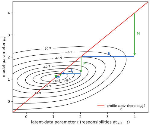
fig_8_7. Reproduces Hastie, Tibshirani and Friedman (2009), Figure 8.7. Download: PDF · SVGThe view suggests variants: the E step need not update all the latent distributions at once; one may update one \(\gamma_i\) at a time, alternating with M steps, and every such partial step still increases \(F\) (Neal and Hinton, 1998). The companion course has this incremental EM: Algorithm 9.6.
See also (companion courses): the same decomposition with \(\tP=q\) and \(F=\mathcal L(q,\theta)\), and the EM lower-bound demo, in Bayesian and Probabilistic Machine Learning, Section 9.4; Foundations of Deep Learning, Result 15.11.
8.6 MCMC for Sampling from the Posterior
pp. 279–282 To make inferences from a posterior one would like to draw samples from it, which for all but simple models is hard. Markov chain Monte Carlo (MCMC) produces a dependent sequence whose distribution converges to the target. Gibbs sampling, the simplest MCMC method, is closely related to EM: it samples from conditional distributions where EM maximises over them.
Algorithm 8.3 (Gibbs sampler) p. 279
- Take some initial values \(U_k^{(0)}\), \(k=1,2,\dots,K\).
- Repeat for \(t=1,2,\dots\): for \(k=1,2,\dots,K\) generate \(U_k^{(t)}\) from \[\Pr\big(U_k^{(t)}\given U_1^{(t)},\dots,U_{k-1}^{(t)},U_{k+1}^{(t-1)},\dots,U_K^{(t-1)}\big)\].
- Continue step 2 until the joint distribution of \((U_1^{(t)},\dots,U_K^{(t)})\) does not change.
Result 8.10 (the target is a stationary distribution of the Gibbs sampler) p. 279
If \((U_1,\dots,U_K)\) has the joint distribution \(p\), then after one Gibbs update of any coordinate it still has distribution \(p\); so one full sweep of Algorithm 8.3 leaves \(p\) invariant. If in addition the chain is irreducible and aperiodic (for example, if all full conditionals are positive everywhere), the distribution of \(U^{(t)}\) converges to \(p\) from any start, and averages along the chain converge to expectations under \(p\).
Proof of invariance; convergence by reference
Let \(U\sim p\) and replace \(U_k\) by a draw \(U_k'\) from \(p(u_k\given u_{-k})\), where \(u_{-k}\) denotes the other coordinates. The marginal of \(U_{-k}\) is unchanged, \(p(u_{-k})\), and given \(U_{-k}=u_{-k}\) the new coordinate has density \(p(u_k'\given u_{-k})\); so the new joint density is \(p(u_{-k})p(u_k'\given u_{-k})=p(u_{-k},u_k')\). A sweep is a composition of \(K\) such updates, each preserving \(p\). (This is the sense of the book's remark that the steps "leave the marginal distributions unchanged".) Each single update is a Metropolis–Hastings step whose acceptance probability is 1, and the convergence theorem for chains that are irreducible and aperiodic with a stationary distribution then applies; the companion courses prove both facts: Result 11.20 and Result 11.17 of Bayesian and Probabilistic Machine Learning, Result 14.10 of Foundations of Deep Learning. ∎
One does not need the conditional densities in closed form, only the ability to sample from them. After a burn-in period, the marginal of any subset of variables can be estimated from the draws. If the conditional density of \(U_k\) is known, a better estimate of the marginal density of \(U_k\) averages it over the draws:
\[ \widehat{\Pr}_{U_k}(u)=\frac1{M-m+1}\sum_{t=m}^M\Pr\big(u\given U_\ell^{(t)},\ell\neq k\big). \tag{8.50} \]Result 8.11 (the Rao–Blackwell estimate (8.50)) p. 280; Exercise 8.3
If the chain is stationary, each term of (8.50) is an unbiased estimate of the marginal density \(p_{U_k}(u)\), and its variance is no larger than that of any kernel estimate built from draws of \(U_k\) with the same expectation. Under the convergence of Result 8.10 the average converges to \(p_{U_k}(u)\) at every \(u\).
Proof
By Exercise 8.3's relation \(\Pr(A)=\int\Pr(A\given B)\,\d\Pr(B)\) with \(B=U_{-k}\): \[\E\big[p(u\given U_{-k})\big]=\int p(u\given u_{-k})p(u_{-k})\,\d u_{-k}=p_{U_k}(u).\] For the variance, a density estimate from the draws \(U_k^{(t)}\), \(K_h(u-U_k^{(t)})\), has conditional expectation \[\E[K_h(u-U_k)\given U_{-k}]=\int K_h(u-v)p(v\given U_{-k})\d v\], and by the law of total variance \[\Var K_h(u-U_k)\ge\Var\E[K_h(u-U_k)\given U_{-k}]\]; as \(h\to0\) the right side becomes the variance of \(p(u\given U_{-k})\). Conditioning removes the noise of the draw of \(U_k\) itself (the Rao–Blackwell theorem). The ergodic average converges by Result 8.10. On a bivariate normal Gibbs sampler with correlation 0.8, (8.50) is within 0.002 of the exact \(\N(0,1)\) marginal after 20000 sweeps; for the mixture, see Figure 8.S2. ∎
For Bayesian inference the target is the posterior. EM and Gibbs sampling meet when the latent data \(\bZ^m\) are treated as one more set of parameters. For the mixture, take the parameters to be \((\theta,\Delta)\) and, to keep the connection clean, fix \(\sigma_1^2,\sigma_2^2,\pi\) at their maximum likelihood values, so that only \(\mu_1,\mu_2\) are unknown, with a flat prior.
Filling the gap 8.7: the full conditionals of the mixture p. 280
With \(\sigma_1^2,\sigma_2^2,\pi\) fixed and a flat prior on \((\mu_1,\mu_2)\), the joint posterior of \((\mu_1,\mu_2,\Delta)\) is proportional to the complete-data likelihood \(\exp\ell_0\) of (8.40). Its full conditionals are
\[ \Delta_i\given\mu,\by\sim\text{Bernoulli}\big(\gamma_i(\theta)\big)\ \text{independently},\qquad\mu_k\given\Delta,\by\sim\N\Big(\bar y_k,\;\frac{\sigma_k^2}{n_k}\Big), \]where \(n_2=\sum_i\Delta_i\), \(n_1=N-n_2\), and \(\bar y_k\) is the mean of the \(n_k\) points in component \(k\).
Derivation, and why the prior must be proper
For fixed \(\mu\), \(\exp\ell_0\) is a product over \(i\) of \(\{(1-\pi)\phi_{\theta_1}(y_i)\}^{1-\Delta_i}\{\pi\phi_{\theta_2}(y_i)\}^{\Delta_i}\), so the \(\Delta_i\) are independent with \(\Pr(\Delta_i=1)\) given by (8.42). For fixed \(\Delta\), the factor involving \(\mu_2\) is \[\prod_{i:\Delta_i=1}\exp\{-(y_i-\mu_2)^2/(2\sigma_2^2)\}\propto\exp\{-n_2(\mu_2-\bar y_2)^2/(2\sigma_2^2)\}\], using \[\sum(y_i-\mu)^2=\sum(y_i-\bar y)^2+n(\mu-\bar y)^2\]: a normal density with mean \(\bar y_2\) and variance \(\sigma_2^2/n_2\). The same for \(\mu_1\).
If \(n_k=0\) the factor is constant in \(\mu_k\), and with a flat prior the conditional is not a distribution. Worse, the joint posterior is then improper: the configurations with an empty component contribute \(\int\d\mu_k=\infty\) to the normalising constant, so "all the mixing weight on one component" dominates, which is the degeneracy the book warns about. A proper prior on the means (or a sampler that keeps \(\mu_k\) unchanged when its component is empty, as in the code) avoids this; with twenty well-separated points it does not arise in practice.
Algorithm 8.4 (Gibbs sampling for mixtures) p. 281
- Take some initial values \(\theta^{(0)}=(\mu_1^{(0)},\mu_2^{(0)})\).
- Repeat for \(t=1,2,\dots\):
- For \(i=1,2,\dots,N\) generate \(\Delta_i^{(t)}\in\{0,1\}\) with \(\Pr(\Delta_i^{(t)}=1)=\hat\gamma_i(\theta^{(t)})\), from (8.42).
- Set \(\hmu_1=\dfrac{\sum_{i=1}^N(1-\Delta_i^{(t)})\cdot y_i}{\sum_{i=1}^N(1-\Delta_i^{(t)})}\), \(\hmu_2=\dfrac{\sum_{i=1}^N\Delta_i^{(t)}\cdot y_i}{\sum_{i=1}^N\Delta_i^{(t)}}\), and generate \(\mu_1^{(t)}\sim\N(\hmu_1,\hs_1^2)\) and \(\mu_2^{(t)}\sim\N(\hmu_2,\hs_2^2)\) (as printed; see the note below).
- Continue step 2 until the joint distribution of \((\Delta^{(t)},\mu_1^{(t)},\mu_2^{(t)})\) does not change.
Steps 2(a) and 2(b) are the E and M steps of EM with sampling in place of averaging and maximising: 2(a) draws the labels from the distribution whose mean EM uses, and 2(b) draws the means from the distribution whose mode EM takes.
Note on the book: the variance in step 2(b) of Algorithm 8.4 p. 281, Figure 8.8
By Filling the gap 8.7 the full conditional of \(\mu_k\) under a flat prior is \(\N(\hmu_k,\hs_k^2/n_k)\), not \(\N(\hmu_k,\hs_k^2)\): the uncertainty of a mean of \(n_k\approx10\) points is \(\hs_k/\sqrt{n_k}\approx0.29\), not \(\hs_k\approx0.9\). The printed version does not sample from the posterior. Figure 8.8 of the book was evidently made with it: its traces scatter by about one unit around the maximum likelihood values (reproduced below, standard deviation 0.93 for \(\mu_2\)). The over-dispersed chain also wanders across to the mirror-image mode: run for 20000 iterations, it has the two labels swapped 49.8% of the time, while the exact sampler never swaps them. Drawn correctly, the posterior means are \(\E(\mu_1\given\by)=4.663\) and \(\E(\mu_2\given\by)=1.089\) with standard deviations 0.33 and 0.30, in agreement with the posterior computed by brute-force integration over a grid (4.660, 1.086, sd 0.296).
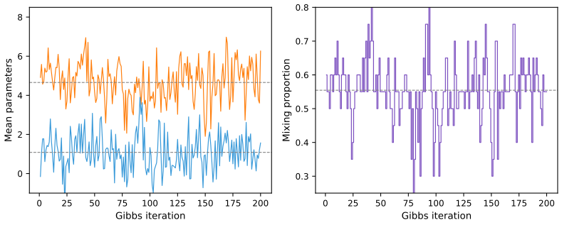
fig_8_8. Reproduces Hastie, Tibshirani and Friedman (2009), Figure 8.8. Download: PDF · SVG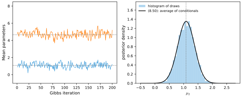
fig_8_s2. Download: PDF · SVGA more realistic analysis puts priors on \(\sigma_1^2,\sigma_2^2\) and \(\pi\) too and adds Gibbs steps for them. With conjugate priors, \(\pi\given\Delta\sim\text{Beta}(\alpha+n_2,\alpha+n_1)\) and \((\mu_k,\sigma_k^2)\given\Delta\) is normal-inverse-gamma: \[\sigma_k^2\sim\text{Inv-Gamma}\big(a_0+\tfrac{n_k}2,\,b_0+\tfrac12S_k+\tfrac{\kappa_0n_k}{2(\kappa_0+n_k)}(\bar y_k-m_0)^2\big)\] and \[\mu_k\given\sigma_k^2\sim\N\big(\frac{\kappa_0m_0+n_k\bar y_k}{\kappa_0+n_k},\frac{\sigma_k^2}{\kappa_0+n_k}\big)\], with \(S_k\) the within-component sum of squares (the standard conjugate update for a normal sample, applied to the points currently in component \(k\)). When the prior treats the two components alike the posterior is symmetric under swapping the labels, and a well-mixing sampler should switch labels; summaries must then be label-free, for example the larger and the smaller of the two means.
Gibbs sampling is one of many MCMC methods; the Metropolis–Hastings algorithm needs no conditional structure at all. These methods have been applied to Gaussian process models and neural networks (Neal, 1996).
See also (companion courses): Bayesian and Probabilistic Machine Learning, Section 11.3 (Gibbs sampling, with the MCMC demo) and Foundations of Deep Learning, Section 14.2.4.
8.7 Bagging
pp. 282–288 The bootstrap was used so far to assess an estimate. Bagging (bootstrap aggregation; Breiman, 1996a) uses it to improve the estimate. For bootstrap samples \(\bZ^{*b}\), \(b=1,\dots,B\), fit the model to each, obtaining \(\hf^{*b}(x)\), and average:
\[ \hf_{\bag}(x)=\frac1B\sum_{b=1}^B\hf^{*b}(x). \tag{8.51} \]With \(\hat{\mathcal P}\) the empirical distribution of the training pairs, the "true" bagging estimate is \(\E_{\hat{\mathcal P}}\hf^*(x)\), of which (8.51) is a Monte Carlo approximation. Bagging changes nothing for an estimator that is linear in the data under the parametric bootstrap: by Result 8.1 (and Exercise 8.4), bagging the B-spline smoother with (8.6) returns \(\hmu(x)\) as \(B\to\infty\). With the nonparametric bootstrap it is only approximately so (with \(B=4000\) the bagged curve stays within 0.04 of \(\hmu\) away from the ends), because the fit is not linear in the resampled \(x_i\). Bagging matters for nonlinear, adaptive procedures such as trees.
For a \(K\)-class classifier \(\hat G(x)\), write it as the indicator vector \(\hf(x)\) with a single one; then \(\hf_{\bag}(x)=(p_1(x),\dots,p_K(x))\) records the proportion of trees voting for each class, and the bagged classifier takes the majority vote, \(\hat G_{\bag}(x)=\argmax_k\hf_{\bag}(x)\). The vote proportions are not class probabilities: if \(\Pr(Y=1\given x)=0.75\) and every bootstrap classifier predicts class 1, then \(p_1(x)=1\). Averaging the trees' own class-proportion estimates instead gives better probability estimates and often a lower-variance classifier.
See also (companion courses): Algorithm 14.1 of Bayesian and Probabilistic Machine Learning and the trees and committees demo (bagging regression trees); Foundations of Deep Learning, Result 9.11 (committee error).
8.7.1 Example: Trees with Simulated Data
pp. 283–285 A training sample of \(N=30\) has two classes and \(p=5\) standard Gaussian features with pairwise correlation 0.95, and \(\Pr(Y=1\given x_1\le0.5)=0.2\), \(\Pr(Y=1\given x_1>0.5)=0.8\); the Bayes error is 0.2. A test sample has 2000 points. Classification trees are grown on the training sample and on each of 200 bootstrap samples, without pruning. Here the trees are grown on the deviance with the default stopping rules of the R package tree, and our implementation reproduces that package's splits exactly on test data sets.
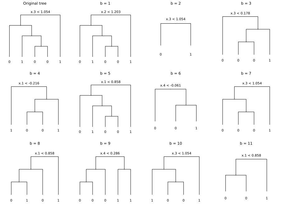
fig_8_9. Reproduces Hastie, Tibshirani and Friedman (2009), Figure 8.9. Download: PDF · SVG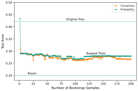
fig_8_10. Reproduces Hastie, Tibshirani and Friedman (2009), Figure 8.10. Download: PDF · SVGResult 8.12 (aggregation cannot increase squared error) p. 285, (8.52)
Let the training pairs be drawn from \(\mathcal P\), fix \(x\), let \(Y\) be a new response at \(x\), independent of the training data, and let \(f_{\ag}(x)=\E_{\mathcal P}\hf^*(x)\) be the ideal aggregate over training sets drawn from the population. Then
\[ \E_{\mathcal P}[Y-\hf^*(x)]^2=\E_{\mathcal P}[Y-f_{\ag}(x)]^2+\E_{\mathcal P}[\hf^*(x)-f_{\ag}(x)]^2\ge\E_{\mathcal P}[Y-f_{\ag}(x)]^2. \tag{8.52} \]Proof
Expand \([Y-f_{\ag}+f_{\ag}-\hf^*]^2\). The cross term is \(2\E[(Y-f_{\ag})(f_{\ag}-\hf^*)]\). Since \(Y\) is independent of the training data, and \(f_{\ag}(x)\) is a constant, this factorises: \[2\E[Y-f_{\ag}]\cdot\E[f_{\ag}-\hf^*]=2\E[Y-f_{\ag}]\cdot0\], because \(\E\hf^*(x)=f_{\ag}(x)\) by definition. The book writes the step without comment; independence of \(Y\) from the training sample is what makes it work. The extra term is the variance of \(\hf^*(x)\) around its mean. A simulation with a two-piece regression stump confirms the decomposition to within simulation error. ∎
So true population aggregation never increases mean squared error, which suggests that bagging, which aggregates over the empirical distribution instead, will often decrease it. Under 0–1 loss the argument fails, because bias and variance do not add: bagging a good classifier can make it better, but bagging a bad one can make it worse. The book's extreme example: if \(Y=1\) for all \(x\) and a randomised classifier predicts 1 with probability 0.4 and 0 with probability 0.6 (for all \(x\)), its error is 0.6, while the majority vote of many independent copies predicts 0 and has error 1 (for 11 votes the error is already 0.75, for 101 votes 0.98). The next result says exactly when aggregation helps.
Result 8.13 (when aggregation helps under 0–1 loss) pp. 285–286
Two classes. At a fixed \(x\), let \(\eta(x)=\Pr(Y=1\given x)\), \(G^*(x)\) the Bayes class and \(e_B(x)=\min(\eta,1-\eta)\) the Bayes error, and let \(p(x)\) be the probability (over training sets) that the classifier \(\hat G(x)\) predicts \(G^*(x)\). Then
\[ \Pr\{\hat G(x)\ne Y\}=e_B(x)+\big(1-p(x)\big)\,|2\eta(x)-1|. \]The aggregated classifier \(G_{\ag}(x)\), the majority vote over training sets drawn from the population, predicts \(G^*(x)\) if \(p(x)>\frac12\) and the other class if \(p(x)<\frac12\). Its error is \(e_B(x)\) in the first case and \(e_B(x)+|2\eta(x)-1|\) in the second. So aggregation lowers the error at every \(x\) where the classifier is right more often than not, and raises it at every \(x\) where it is wrong more often than not.
Proof
Given the training data, \(\hat G(x)\) is a fixed label and \(Y\) is independent of it. If \(\hat G(x)=G^*(x)\) the error is \(e_B\); otherwise it is \(1-e_B=e_B+|2\eta-1|\). Averaging over training sets gives \(p\,e_B+(1-p)(e_B+|2\eta-1|)\). The majority vote of infinitely many independent draws of \(\hat G(x)\) is, by the law of large numbers, the label with probability above \(\frac12\), so \(G_{\ag}(x)=G^*(x)\) iff \(p(x)>\frac12\). Compare \(1-p\) with 0 or 1. ∎
In the simulation of Section 8.7.1, \(e_B=0.2\) and \(|2\eta-1|=0.6\) everywhere, so the expected test error given the test inputs is \(0.2+0.6\times\)(fraction of test points where the classifier disagrees with the Bayes rule); for Figure 8.10 this is 0.412 for the single tree and 0.267 for the vote. Bagging uses bootstrap samples, not the population, so it only approximates \(G_{\ag}\), and the bootstrap trees are not independent; the result explains the direction of the effect, which Figure 8.S6 shows over 60 training sets.
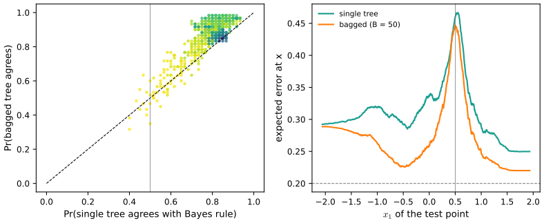
fig_8_s6. Download: PDF · SVGFor classification the effect of bagging can also be seen as a consensus of independent weak learners (Dietterich, 2000a). If the Bayes decision at \(x\) is class 1 and \(B\) independent learners each err with probability \(e<0.5\), the vote for class 1 is \(S_1(x)\sim\Bin(B,1-e)\) and \(\Pr(S_1>B/2)\to1\) as \(B\to\infty\) (for \(e=0.4\): 0.75 with 11 learners, 0.98 with 101). This is the "wisdom of crowds" (Surowiecki, 2004); the catch is independence, which bagged trees do not have. Random forests (Chapter 15) reduce the correlation between the trees.
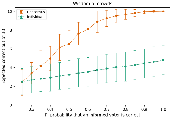
fig_8_11. Reproduces Hastie, Tibshirani and Friedman (2009), Figure 8.11. Download: PDF · SVGFilling the gap 8.8: the individual's expected score in Figure 8.11 p. 287
Derivation
In one category a given member is informed with probability \(15/50=0.3\), and is then correct with probability \(P\); otherwise (probability 0.7) the member is correct with probability \(1/4\). So the probability of a correct vote is \(0.3P+0.175\), and the expected number correct in 10 categories is \(10(0.3P+0.175)\): 2.5 at \(P=0.25\), 3.25 at \(P=0.5\), 4.75 at \(P=1\). The consensus has no simple closed form (the vote counts of the four nominees are multinomial with probabilities that depend on the random number of informed voters), but its limit is clear: the correct nominee's expected vote share exceeds that of each other nominee by \(0.3(P-\frac{1-P}3)\), positive as soon as \(P>\frac14\), so with many voters the plurality is correct with probability tending to 1. With 50 voters the margin needs \(P\) around 0.8 to make the consensus almost always right. ∎
Bagging loses any simple structure: a bagged tree is no longer a tree. Stable procedures such as nearest neighbours are hardly changed by bagging, and the unstable models that bagging helps most are often valued for an interpretability that bagging destroys. Figure 8.12 shows a case where bagging does not help at all: the base classifier is too restricted for averaging to fix.
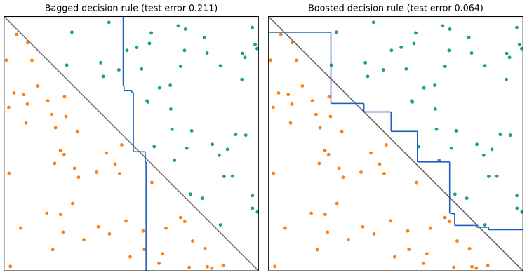
fig_8_12. Reproduces Hastie, Tibshirani and Friedman (2009), Figure 8.12. Download: PDF · SVGNote on the book: "splits near 0" in the discussion of Figure 8.12 p. 286
The text says the single split "splits near 0 (the middle of the range of \(x_1\) or \(x_2\))". With the boundary \(x_1+x_2=1\) drawn as the diagonal of the square, as in the figure, the features range over \([0,1]\) and the middle of the range is \(\frac12\); "near 0" would be the middle only for features on \([-1,1]\), where the boundary \(x_1+x_2=1\) would not be the diagonal. The argument is unaffected: the single split sits in the middle of the range and contributes little away from it.
Bagging estimates the expected class probabilities of the single-split rule. These averaged rules cannot be produced by any single split ("in the same way that a woman cannot have 2.4 children"), so bagging enlarges the model class a little; boosting enlarges it much more.
8.8 Model Averaging and Stacking
pp. 288–290 In the light of Section 8.4, bootstrap values of an estimator are approximate posterior draws, so the bagged estimate (8.51) is an approximate posterior mean, while the fit to the training data corresponds to the posterior mode. The posterior mean minimises posterior expected squared error (Filling the gap 8.9), so it is not surprising that bagging often reduces mean squared error.
More generally, let \(\mathcal M_m\), \(m=1,\dots,M\), be candidate models and \(\zeta\) a quantity of interest, for example \(f(x)\). Then
\[ \Pr(\zeta\given\bZ)=\sum_{m=1}^M\Pr(\zeta\given\mathcal M_m,\bZ)\Pr(\mathcal M_m\given\bZ), \tag{8.53} \] \[ \E(\zeta\given\bZ)=\sum_{m=1}^M\E(\zeta\given\mathcal M_m,\bZ)\Pr(\mathcal M_m\given\bZ). \tag{8.54} \]The Bayesian prediction is a weighted average of the models' predictions with weights equal to the posterior model probabilities,
\[ \Pr(\mathcal M_m\given\bZ)\propto\Pr(\mathcal M_m)\cdot\Pr(\bZ\given\mathcal M_m)\propto\Pr(\mathcal M_m)\cdot\int\Pr(\bZ\given\theta_m,\mathcal M_m)\Pr(\theta_m\given\mathcal M_m)\,\d\theta_m. \tag{8.55} \]Committee methods take an unweighted average (equal model probabilities). The BIC of Section 7.7 approximates \(-2\log\Pr(\bZ\given\mathcal M_m)\), giving the weights \(\propto e^{-\mathrm{BIC}_m/2}\) for models from one parametric family; the full Bayesian recipe (8.55) needs priors on every model's parameters, and the book saw no real evidence that it is worth the effort over BIC.
Filling the gap 8.9: (8.53)–(8.54), and why a posterior mean minimises squared error p. 288
Derivation
(8.53) is the law of total probability over the model index, conditionally on \(\bZ\); (8.54) follows by taking expectations term by term. For any estimate \(a\) computed from the data, \[\E[(\zeta-a)^2\given\bZ]=\Var(\zeta\given\bZ)+(\E(\zeta\given\bZ)-a)^2\], minimised by \(a=\E(\zeta\given\bZ)\). If the model is uncertain, choosing the single most probable model and its prediction gives a larger posterior expected loss than the average (8.54), by exactly \(\big(\E(\zeta\given\bZ)-\E(\zeta\given\mathcal M_{\hat m},\bZ)\big)^2\). The BIC weights follow from Result 4.19 of the companion course: \[\log\Pr(\bZ\given\mathcal M_m)=-\frac12\mathrm{BIC}_m+O(1)\], so with equal prior model probabilities \[\Pr(\mathcal M_m\given\bZ)\approx e^{-\mathrm{BIC}_m/2}/\sum_\ell e^{-\mathrm{BIC}_\ell/2}\]. ∎
See also (companion course): Bayesian and Probabilistic Machine Learning, Section 14.1 (Bayesian model averaging is not model combination, and Result 14.1: it concentrates on one model as \(N\) grows).
From a frequentist viewpoint, given predictions \(\hf_1(x),\dots,\hf_M(x)\), seek the weights that minimise the expected squared error at \(x\),
\[ \hat w=\argmin_w\E_{\mathcal P}\Big[Y-\sum_{m=1}^Mw_m\hf_m(x)\Big]^2, \tag{8.56} \]where the data set \(\bZ\) and the target \(Y\) are random from \(\mathcal P\). The solution is the population linear regression of \(Y\) on \(\hat F(x)^\T\equiv[\hf_1(x),\dots,\hf_M(x)]\):
\[ \hat w=\E_{\mathcal P}[\hat F(x)\hat F(x)^\T]^{-1}\E_{\mathcal P}[\hat F(x)Y], \tag{8.57} \]and the full regression has smaller error than any single model,
\[ \E_{\mathcal P}\Big[Y-\sum_{m=1}^M\hat w_m\hf_m(x)\Big]^2\le\E_{\mathcal P}\big[Y-\hf_m(x)\big]^2\quad\forall m, \tag{8.58} \]so combining never hurts at the population level. (8.57) is the normal equation of the quadratic (8.56) (assuming the second-moment matrix is invertible), and (8.58) holds because the unit vector \(e_m\) is one of the candidates in the minimisation.
In practice the population regression is replaced by the regression on the training set, which can fail badly:
Result 8.14 (least squares on fitted values picks the largest model) p. 290
Let \(\hf_m\) be the least squares fit on a set of inputs \(S_m\) (with intercept), \(m=1,\dots,M\), with \(S_1\subseteq S_2\subseteq\dots\subseteq S_M\) (for example best subsets that happen to be nested, or simply nested models). The least squares regression of \(\by\) on the fitted vectors \(\hf_1,\dots,\hf_M\) has the solution \(w=e_M\): all the weight on the largest model. If the subsets are not nested but all lie in \(S_M\), the same holds whenever the fitted vectors are linearly independent.
Proof
Each \(\hf_m=\mathbf P_m\by\) is the projection of \(\by\) onto the column space \(\mathcal C_m\) of its design matrix, and \(\mathcal C_m\subseteq\mathcal C_M\). The residual \(\by-\hf_M\) is orthogonal to \(\mathcal C_M\), hence to every \(\hf_m\). So \(w=e_M\) satisfies the normal equations \(\hat F^\T(\by-\hat Fw)=0\), and it is the unique solution when the columns of \(\hat F\) are linearly independent. Any combination lies in \(\mathcal C_M\), and \(\hf_M\) is already the closest point of \(\mathcal C_M\) to \(\by\). On the prostate data with the best subsets of sizes 0 to 8, the regression returns \(w=e_9\) to machine precision (all eight best subsets are nested there). ∎
The trouble is that the models have not been put on an equal footing: their training fits reward complexity. Stacked generalisation (stacking; Wolpert, 1992) uses leave-one-out predictions \(\hf_m^{-i}(x)\), from model \(m\) fitted without observation \(i\):
\[ \hat w^{\st}=\argmin_w\sum_{i=1}^N\Big[y_i-\sum_{m=1}^Mw_m\hf_m^{-i}(x_i)\Big]^2, \tag{8.59} \]and the final prediction is \(\sum_m\hat w^{\st}_m\hf_m(x)\). Better results are usually obtained with \(w_m\ge0\) and \(\sum_mw_m=1\), which matches the interpretation of the weights as model probabilities in (8.54).
Result 8.15 (computing the stacking weights) p. 290
- For a linear fit \(\hf_m=\bS_m\by\) that is least squares on its own inputs, \(\hf_m^{-i}(x_i)=y_i-\dfrac{y_i-\hf_m(x_i)}{1-(\bS_m)_{ii}}\): one fit per model gives all \(N\) leave-one-out predictions.
- With \(\bF\) the \(N\times M\) matrix of leave-one-out predictions, unconstrained stacking is the least squares regression \(\hat w^{\st}=(\bF^\T\bF)^{-1}\bF^\T\by\).
- With the constraints \(w\ge0\), \(\sum w_m=1\), (8.59) is a convex quadratic programme; \(w\) is optimal iff there is \(\lambda\) with \(g_m=\lambda\) where \(w_m>0\) and \(g_m\ge\lambda\) where \(w_m=0\), \(g=-2\bF^\T(\by-\bF w)\) being the gradient.
- Restricting \(w\) to the unit vectors \(e_m\) turns (8.59) into the leave-one-out cross-validation error of model \(m\): stacking contains leave-one-out model selection as a special case.
Proof
(1) is the leave-one-out identity for least squares (Section 7.10 of the book; for linear smoothers it was proved in Chapter 6, Result 6.6): deleting observation \(i\) and refitting gives the same fit as replacing \(y_i\) by its own deleted prediction \(\hf^{-i}(x_i)\), so \(\hf^{-i}(x_i)=\sum_{j\ne i}S_{ij}y_j+S_{ii}\hf^{-i}(x_i)\), and solving gives the formula. (2) is ordinary least squares with \(\bF\) as design. (3) The objective is convex and the constraints are linear, so the Karush–Kuhn–Tucker conditions are necessary and sufficient: with multiplier \(\lambda\) for \(\sum w=1\) and \(\nu_m\ge0\) for \(w_m\ge0\), stationarity is \(g_m=\lambda+\nu_m\) with \(\nu_mw_m=0\), which is the statement. (4) \[\sum_i(y_i-e_m^\T\bF_i)^2=\sum_i(y_i-\hf_m^{-i}(x_i))^2\]. The code checks (1) against \(N\) refits and (3) at its solution. ∎
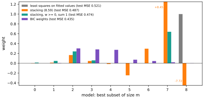
fig_8_s5. Download: PDF · SVGStacking is more general than linear regression on the predictions: any learning method can combine the models, and the weights may depend on \(x\). Learning methods are thus "stacked" on top of one another. LeBlanc and Tibshirani (1996) describe bootstrap variants.
8.9 Stochastic Search: Bumping
pp. 290–292 Bumping (Tibshirani and Knight, 1999) does not average; it uses the bootstrap to search for a better single model. Draw bootstrap samples \(\bZ^{*1},\dots,\bZ^{*B}\), fit the model to each, and keep the one that fits the original training data best; for squared error,
\[ \hat b=\argmin_b\sum_{i=1}^N\big[y_i-\hf^{*b}(x_i)\big]^2. \tag{8.60} \]The original sample is included among the candidates, so bumping can return the original model. Perturbing the data moves the fitting procedure around model space: if a few points push the procedure to a poor solution, a bootstrap sample that omits them may lead to a better one.
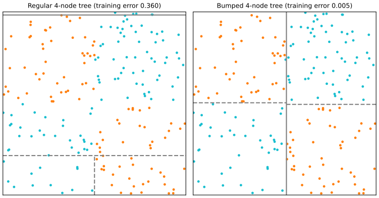
fig_8_13. Reproduces Hastie, Tibshirani and Friedman (2009), Figure 8.13. Download: PDF · SVGBootstrap sampling breaks the balance of the classes, and with a reasonable number of samples one of them produces a first split near \(x_1=0\) or \(x_2=0\). Adding noise features makes the greedy algorithm worse, since it cannot tell \(x_1,x_2\) from the noise. Two practical points. Because the candidates are compared on the training data, they must have the same complexity (here, the same number of leaves), or the largest would always win (compare Result 8.14). And bumping can optimise an awkward criterion: fit each bootstrap sample with a convenient criterion and choose among the fits by the one that matters.
Exercises
All 7 exercises of Chapter 8 (Hastie, Tibshirani and Friedman, 2009, pp. 293–294), restated in my own words, with complete solutions (hidden).
Exercise 8.1. Let \(r(y)\) and \(q(y)\) be probability densities. Using Jensen's inequality, \(\E\varphi(X)\ge\varphi(\E X)\) for convex \(\varphi\), show that
\[ \E_q\log[r(Y)/q(Y)] \tag{8.61} \]is maximised over \(r\) by \(r=q\). Deduce that \(R(\theta,\theta)\ge R(\theta',\theta)\), as used after (8.46).
Solution
\(\varphi=-\log\) is strictly convex, so with \(Y\sim q\) and \(X=r(Y)/q(Y)\) (defined where \(q>0\)),
\[ \E_q\log\frac{r(Y)}{q(Y)}\le\log\E_q\frac{r(Y)}{q(Y)}=\log\int_{q>0}r(y)\,\d y\le\log1=0. \]The value 0 is attained at \(r=q\), so \(r=q\) is a maximiser. It is the only one: equality in Jensen's inequality for a strictly convex function requires \(r(Y)/q(Y)\) to be constant \(q\)-almost surely, and then \(\int_{q>0}r=1\) forces the constant to be 1, so \(r=q\) almost everywhere. (The quantity \(-\E_q\log(r/q)\) is the Kullback–Leibler divergence \(\KL(q\,\|\,r)\).)
For EM, \[R(\theta',\theta)=\E[\log\Pr(\bZ^m\given\bZ,\theta')\given\bZ,\theta]\]. Put \(q=\Pr(\cdot\given\bZ,\theta)\) and \(r=\Pr(\cdot\given\bZ,\theta')\): then \[R(\theta',\theta)-R(\theta,\theta)=\E_q\log(r/q)\le0\]. (For discrete latent data, as in the mixture, replace integrals by sums; the argument is unchanged.)
Exercise 8.2. Maximise \(F(\theta',\tP)\) of (8.48) over distributions \(\tP(\bZ^m)\ge0\) with \(\sum_{\bZ^m}\tP(\bZ^m)=1\), using a Lagrange multiplier, and show that the maximiser is \(\tP(\bZ^m)=\Pr(\bZ^m\given\bZ,\theta')\), as in (8.49).
Solution
Write \(z\) for the values of \(\bZ^m\) (finitely many, or countably many with the same argument) and \(p_z=\tP(z)\). Then \[F=\sum_zp_z\,\ell_0(\theta';\bZ,z)-\sum_zp_z\log p_z\]. Ignore the constraints \(p_z\ge0\) for the moment and form \(\mathcal L=F+\lambda(\sum_zp_z-1)\). Setting \[\partial\mathcal L/\partial p_z=\ell_0(\theta';\bZ,z)-\log p_z-1+\lambda=0\] gives
\[ p_z=e^{\lambda-1}\exp\ell_0(\theta';\bZ,z)=e^{\lambda-1}\Pr(\bZ,z\given\theta'). \]The constraint \(\sum p_z=1\) fixes \[e^{\lambda-1}=1/\sum_z\Pr(\bZ,z\given\theta')=1/\Pr(\bZ\given\theta')\], so \[p_z=\Pr(\bZ,z\given\theta')/\Pr(\bZ\given\theta')=\Pr(z\given\bZ,\theta')\]. This is positive, so the ignored constraints are inactive. \(F\) is strictly concave in \(p\) (a linear term plus the strictly concave entropy) on a convex set, so the stationary point is the unique global maximum. Its value is \[\sum_zp_z[\log\Pr(\bZ,z\given\theta')-\log\Pr(z\given\bZ,\theta')]=\log\Pr(\bZ\given\theta')=\ell(\theta';\bZ)\]. For the mixture the maximisation runs over the twenty \(\gamma_i\) separately and gives (8.42) (checked numerically to four decimals).
Exercise 8.3. Justify the estimate (8.50) using \(\Pr(A)=\int\Pr(A\given B)\,\d\Pr(B)\).
Solution
Take \(A=\{U_k\in[u,u+\d u)\}\) and \(B=U_{-k}=(U_\ell)_{\ell\ne k}\): the identity says \[p_{U_k}(u)=\int p(u\given u_{-k})\,p(u_{-k})\,\d u_{-k}=\E\,p(u\given U_{-k}).\] Once the Gibbs chain is stationary each \(U^{(t)}\) has the joint distribution, so each \(U^{(t)}_{-k}\) is a draw from the marginal of \(U_{-k}\), and every term of (8.50) has expectation \(p_{U_k}(u)\). The terms are dependent, but the ergodic theorem for the chain (Result 8.10) gives convergence of the average; the burn-in \(t\lt m\) is discarded so that the early, non-stationary terms do not bias it in finite runs. Compared with a histogram or kernel estimate of the draws \(U_k^{(t)}\), (8.50) is smoother and, by the law of total variance, less variable (Result 8.11). In the mixture example it is within 0.003 of the exact posterior density of \(\mu_2\) (Figure 8.S2); for a bivariate normal with correlation 0.8 it is within 0.002 of the \(\N(0,1)\) marginal.
Exercise 8.4. Bag the B-spline smoother \(\hmu(x)\) of Section 8.2.1 with the parametric bootstrap (8.6). Show that the bagged estimate converges to \(\hmu(x)\) as \(B\to\infty\).
Solution
Each bootstrap fit is \(\hf^{*b}(x)=\bm l(x)^\T\by^{*b}\) with \(\bm l(x)^\T=h(x)^\T(\bH^\T\bH)^{-1}\bH^\T\) and \(\by^{*b}=\bH\hb+\varepsilon^{*b}\), the \(\varepsilon^{*b}\) independent \(\N(0,\hs^2\bI)\). By Result 8.1, the \(\hf^{*b}(x)\) are independent \(\N(\hmu(x),\widehat{\mathrm{se}}^2)\), so
\[ \hf_{\bag}(x)=\frac1B\sum_b\hf^{*b}(x)=\hmu(x)+\bm l(x)^\T\bar\varepsilon^*,\qquad\hf_{\bag}(x)\sim\N\big(\hmu(x),\widehat{\mathrm{se}}[\hmu(x)]^2/B\big), \]which converges to \(\hmu(x)\) (almost surely, by the strong law, and uniformly in \(x\) on the compact range because \(\bar\varepsilon^*\to0\) and \(\bm l(x)\) is bounded). The "true" bagging estimate \(\E^*\hf^*(x)=\hmu(x)\) equals the original fit exactly; bagging changes only estimators that are nonlinear in the resampled quantities. With \(B=4000\) the standardised deviations \((\hf_{\bag}-\hmu)/(\widehat{\mathrm{se}}/\sqrt B)\) on the 301-point grid are all below 2.4 in absolute value. With the nonparametric bootstrap the fit is linear in \(\by\) but not in the resampled \(x_i\), and the bagged curve differs slightly from \(\hmu\) (by up to 0.04 away from the ends).
Exercise 8.5. Generalise each loss function of Figure 10.4 (misclassification, exponential, binomial deviance, squared error, support vector hinge) to more than two classes, and design a plot to compare them.
Solution
For two classes with \(y\in\{-1,1\}\) the losses of Figure 10.4 are functions of the margin \(yf\): \(I(yf<0)\), \(e^{-yf}\), \(\log(1+e^{-2yf})\), \((1-yf)^2\), \((1-yf)_+\). For \(K\) classes use a score vector \(f=(f_1,\dots,f_K)\) with \(\sum_kf_k=0\) (scores are defined up to a common shift), classify by \(\argmax_kf_k\), and let the multiclass margin be \(m=f_y-\max_{k\ne y}f_k\). With the coding \(\tilde y_k=1\) for \(k=y\) and \(\tilde y_k=-1/(K-1)\) otherwise:
- Misclassification: \(I(m<0)\).
- Multinomial deviance: \(-\log\frac{e^{f_y}}{\sum_ke^{f_k}}=\log\sum_ke^{f_k-f_y}\). For \(K=2\), \(f=(f,-f)\), this is \(\log(1+e^{-2yf})\).
- Exponential (Zhu, Zou, Rosset and Hastie, 2009): \(\exp(-\tfrac1K\tilde y^\T f)\), which equals \(e^{-f_y/(K-1)}\) when \(\sum f_k=0\); for \(K=2\) it is \(e^{-yf}\). Its population minimiser is \[f_k=(K-1)\{\log p_k-\frac1K\sum_\ell\log p_\ell\}\], so it is Fisher consistent like the deviance.
- Squared error: \(\sum_k(\tilde y_k-f_k)^2\) (or with 0/1 indicator targets).
- Hinge: either Crammer and Singer's \((1-m)_+\), which looks only at the runner-up, or Lee, Lin and Wahba's \(\sum_{k\ne y}(f_k+\frac1{K-1})_+\); both reduce to \((1-yf)_+\) for \(K=2\) (up to the scaling of the margin).
Every loss depends on \(K-1\) free scores, so one curve no longer tells the whole story. A good plot has two panels: (a) each loss against the margin \(m\) along the ray where all wrong-class scores are equal (then everything is a function of \(m\) alone), normalised to 1 at \(m=0\); (b) at a fixed margin, each loss against the spread of the wrong-class scores. Figure 8.S3 does this for \(K=3\). Panel (a) reproduces the shape of Figure 10.4: exponential and deviance are smooth and decreasing, the hinge is zero beyond margin 1, squared error rises again for large margins (it penalises being "too right"). Panel (b) shows the new multiclass feature: the Crammer–Singer hinge ignores the third class, the deviance and the exponential loss fall as the third class is pushed further down, and the sum of hinges grows because, after centring, pushing one wrong class down pushes the other up.
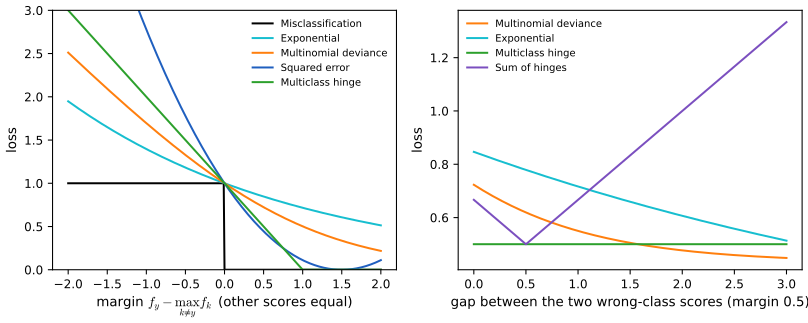
Figure 8.S3 (supplementary, Exercise 8.5). Multiclass losses for \(K=3\), scores summing to zero. Left: along the ray with equal wrong-class scores, as functions of the margin \(f_y-\max_{k\ne y}f_k\), each scaled to equal 1 at margin 0. Right: at margin 0.5, as functions of the gap between the two wrong-class scores. Code: fig_8_s3. Download: PDF · SVGExercise 8.6. For the bone mineral density data of Figure 5.6: (a) fit a cubic smoothing spline to the relative change in spinal BMD against age, choosing the amount of smoothing by cross-validation, and construct pointwise 90% confidence bands; (b) compute the posterior mean and covariance of the true function via (8.28) and compare the posterior bands with (a); (c) compute 100 bootstrap replicates of the fitted curve, as in Figure 8.2, and compare with (a) and (b).
Solution
We use the 259 measurements on females (168 distinct ages). (a) The smoothing spline minimises \(\|\by-\bH\beta\|^2+\lambda\beta^\T\Omega\beta\) over a cubic B-spline basis with knots at the distinct ages, \(\Omega_{jk}=\int h_j''h_k''\) (Chapter 5); the fit is \(\hat\bf=\bS_\lambda\by\), \(\bS_\lambda=\bH(\bH^\T\bH+\lambda\Omega)^{-1}\bH^\T\) (equal to scipy's smoothing spline with the same \(\lambda\) to \(10^{-12}\)). Leave-one-out cross-validation, from one fit per \(\lambda\) via \[\hat f^{-i}(x_i)=y_i-(y_i-\hat f(x_i))/(1-S_{ii})\], chooses \(\lambda=6.80\) (age in years), \(\mathrm{df}=\Tr\bS_\lambda=7.90\). With \(\hs^2=\mathrm{RSS}/(N-\mathrm{df})=0.00123\), the sampling variance of the fit at \(x\) is \(\hs^2\,\bm l(x)^\T\bm l(x)\), \(\bm l(x)^\T=h(x)^\T(\bH^\T\bH+\lambda\Omega)^{-1}\bH^\T\); the band is \(\hat f(x)\pm1.645\) standard errors. It ignores the bias of the smoother, so it is a band for \(\E\hat f(x)\) rather than for \(f(x)\).
(b) Take the prior \(\beta\sim\N(0,\tau\Sigma)\) with \(\Sigma^{-1}=\Omega\) (improper on the linear functions, which \(\Omega\) does not penalise) and \(\tau=\sigma^2/\lambda\). Then (8.27)–(8.28) give the posterior mean \(h(x)^\T(\bH^\T\bH+\lambda\Omega)^{-1}\bH^\T\by\), the smoothing spline itself, and the posterior variance \(\sigma^2h(x)^\T(\bH^\T\bH+\lambda\Omega)^{-1}h(x)\). At the data points the two covariance matrices are \(\sigma^2\bS_\lambda\) (posterior) and \(\sigma^2\bS_\lambda^2\) (sampling). The eigenvalues \(\rho_k\) of \(\bS_\lambda\) lie in \([0,1]\), so \(\rho_k\ge\rho_k^2\) and the posterior band is always the wider one; the difference, \(\sigma^2(\bS_\lambda-\bS_\lambda^2)\), is the prior's allowance for the bias that the frequentist band ignores (Wahba, 1983). Here the posterior half-widths are on average 1.14 times the sampling ones.
(c) Resampling the 259 (age, BMD) pairs 100 times and refitting with the same \(\lambda\) gives the cyan curves of Figure 8.S4; the 5% and 95% points form the bootstrap band. Overall it is 0.79 times as wide as the band of (a), but the ratio is not constant: 1.6 between ages 9 and 13, 0.9 between 13 and 16, and about 0.5 above 16. The reason is heteroscedasticity: the residual standard deviation falls from 0.052 at ages 9–13 to 0.016 above 20, while (a) and (b) use one pooled \(\hs=0.035\). The pairs bootstrap adapts to the local noise; the formula-based bands do not. Two caveats: the bootstrap does not account for bias either, and the data contain repeated measurements on the same girls, so resampling individuals rather than measurements would be more honest.
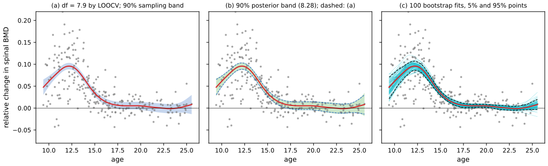
Figure 8.S4 (supplementary, Exercise 8.6). Female spinal bone mineral density. (a) Smoothing spline with \(\lambda\) chosen by leave-one-out cross-validation (df 7.9) and a 90% pointwise sampling band. (b) The 90% posterior band from (8.28) with \(\Sigma^{-1}=\Omega\), \(\tau=\sigma^2/\lambda\); dashed, the band of (a). (c) 100 bootstrap fits with their 5% and 95% points. Code: fig_8_s4. Download: PDF · SVGExercise 8.7 (EM as a minorisation algorithm; Hunter and Lange, 2004; Wu and Lange, 2007). A function \(g(x,y)\) minorises \(f(x)\) if
\[ g(x,y)\le f(x),\qquad g(x,x)=f(x) \tag{8.62} \]for all \(x,y\). Then \(f\) does not decrease under the update
\[ x^{s+1}=\argmax_xg(x,x^s). \tag{8.63} \](Majorisation is the analogue for minimising; the resulting algorithms are MM algorithms.) Show that EM is an MM algorithm with the minoriser \(Q(\theta',\theta)+\log\Pr(\bZ\given\theta)-Q(\theta,\theta)\) of \(\ell(\theta';\bZ)\).
Solution
MM monotonicity. \[f(x^{s+1})\ge g(x^{s+1},x^s)\ge g(x^s,x^s)=f(x^s)\]: the first inequality is minorisation, the second holds because \(x^{s+1}\) maximises \(g(\cdot,x^s)\), and the equality is the touching condition.
EM. Let \[g(\theta',\theta)=Q(\theta',\theta)+\ell(\theta;\bZ)-Q(\theta,\theta)\], with \(\ell(\theta;\bZ)=\log\Pr(\bZ\given\theta)\). By (8.46) at \(\theta'\) and at \(\theta\),
\[ \ell(\theta';\bZ)-g(\theta',\theta)=\big[Q(\theta',\theta)-R(\theta',\theta)\big]-Q(\theta',\theta)-\big[Q(\theta,\theta)-R(\theta,\theta)\big]+Q(\theta,\theta)=R(\theta,\theta)-R(\theta',\theta)\ge0 \]by Exercise 8.1, with equality at \(\theta'=\theta\). So \(g\) minorises \(\ell\). Only \(Q(\theta',\theta)\) depends on \(\theta'\), so \[\argmax_{\theta'}g(\theta',\theta)=\argmax_{\theta'}Q(\theta',\theta)\], the M step; the EM update is the MM update (8.63), and the MM argument gives (8.47) again. The gap \(\ell-g\) is the Kullback–Leibler divergence between the latent-data posteriors at \(\theta\) and \(\theta'\); it is also \(\ell(\theta')-F(\theta',\Pr(\cdot\given\bZ,\theta))\) in the notation of Result 8.9. Checked numerically for 200 random pairs of mixture parameters.
Demonstrations for this chapter
Each demonstration runs in the browser and links back to these notes. The ▶ Demo boxes above open them already set to the case under discussion.
| Demonstration | What you can see | Sections and results |
|---|---|---|
| Bootstrap, maximum likelihood and Bayesian bands | The B-spline smoother of Figures 8.1–8.4 with any number of knots: the least squares band, the nonparametric and parametric bootstrap bands for any \(B\), the posterior band for any prior variance \(\tau\), knots re-chosen by cross-validation in each bootstrap sample, and the distribution of the fit at any \(x_0\). Presets: 1 nonparametric bootstrap (Fig 8.2); 2 parametric bootstrap; 3 \(\tau=1\); 4 \(\tau=1000\) (Fig 8.4); 5 adaptive knots. | 8.2.1–8.2.3, 8.3; Results 8.1, 8.3, 8.4 |
| Gibbs sampling against EM | The mixture of Table 8.1: the EM path on the log-likelihood surface of the two means against the cloud of Gibbs draws; Algorithm 8.4 as printed, the exact conditional, and full Gibbs with priors; traces, the posterior mean density and the Rao–Blackwell estimate (8.50). Presets: 1 Fig 8.8; 2 label switching; 3 exact conditional and (8.50); 4 symmetric start; 5 full Gibbs. | 8.5.1, 8.5.2, 8.6; Result 8.8, 8.11, note on Algorithm 8.4 |
| Bagging classification trees | The simulation of Section 8.7.1 with any sample size, correlation and node size: the original and bootstrap trees, test error against \(B\) for votes and probabilities, and, over 25 training sets, where bagging helps and where it hurts under 0–1 loss. Presets: 1 Figs 8.9–8.10; 2 \(\rho=0\); 3 large nodes; 4 bagging hurts; 5 \(N=200\). | 8.7, 8.7.1; Results 8.12, 8.13 |
Related demonstrations in the companion courses: K-means and EM, the EM lower bound, Metropolis and Gibbs sampling, trees and committees, Bayesian linear regression. The Python code that produces every figure of this page is code/ch08_model_inference_averaging.py (see the code index).
References
- Hastie, T., Tibshirani, R. and Friedman, J. (2009). The Elements of Statistical Learning: Data Mining, Inference, and Prediction, 2nd edition. Springer, New York. Chapter 8, pp. 261–294. hastie.su.domains/ElemStatLearn.
- Breiman, L. (1996a). Bagging predictors. Machine Learning, 24(2), 123–140.
- Breiman, L. (1996b). Stacked regressions. Machine Learning, 24(1), 49–64.
- Cox, D. R. and Hinkley, D. V. (1974). Theoretical Statistics. Chapman and Hall, London.
- Crammer, K. and Singer, Y. (2001). On the algorithmic implementation of multiclass kernel-based vector machines. Journal of Machine Learning Research, 2, 265–292.
- Dempster, A. P., Laird, N. M. and Rubin, D. B. (1977). Maximum likelihood from incomplete data via the EM algorithm. Journal of the Royal Statistical Society, Series B, 39(1), 1–38.
- Dietterich, T. G. (2000a). Ensemble methods in machine learning. In Multiple Classifier Systems, Lecture Notes in Computer Science 1857, Springer, 1–15.
- Efron, B. (1979). Bootstrap methods: another look at the jackknife. The Annals of Statistics, 7(1), 1–26.
- Efron, B. and Tibshirani, R. (1993). An Introduction to the Bootstrap. Chapman and Hall, New York.
- Gelfand, A. E. and Smith, A. F. M. (1990). Sampling-based approaches to calculating marginal densities. Journal of the American Statistical Association, 85(410), 398–409.
- Gelman, A., Carlin, J. B., Stern, H. S. and Rubin, D. B. (1995). Bayesian Data Analysis. Chapman and Hall, London.
- Geman, S. and Geman, D. (1984). Stochastic relaxation, Gibbs distributions, and the Bayesian restoration of images. IEEE Transactions on Pattern Analysis and Machine Intelligence, 6(6), 721–741.
- Hall, P. (1992). The Bootstrap and Edgeworth Expansion. Springer, New York.
- Hunter, D. R. and Lange, K. (2004). A tutorial on MM algorithms. The American Statistician, 58(1), 30–37.
- LeBlanc, M. and Tibshirani, R. (1996). Combining estimates in regression and classification. Journal of the American Statistical Association, 91(436), 1641–1650.
- Lee, Y., Lin, Y. and Wahba, G. (2004). Multicategory support vector machines. Journal of the American Statistical Association, 99(465), 67–81.
- Madigan, D. and Raftery, A. E. (1994). Model selection and accounting for model uncertainty in graphical models using Occam's window. Journal of the American Statistical Association, 89(428), 1535–1546.
- Neal, R. M. (1996). Bayesian Learning for Neural Networks. Springer, New York.
- Neal, R. M. and Hinton, G. E. (1998). A view of the EM algorithm that justifies incremental, sparse, and other variants. In M. I. Jordan (ed.), Learning in Graphical Models, Kluwer, 355–368.
- Rubin, D. B. (1981). The Bayesian bootstrap. The Annals of Statistics, 9(1), 130–134.
- Spiegelhalter, D. J., Best, N. G., Gilks, W. R. and Inskip, H. (1996). Hepatitis B: a case study in MCMC methods. In W. R. Gilks, S. Richardson and D. J. Spiegelhalter (eds.), Markov Chain Monte Carlo in Practice, Chapman and Hall, London.
- Surowiecki, J. (2004). The Wisdom of Crowds. Doubleday, New York.
- Tanner, M. A. and Wong, W. H. (1987). The calculation of posterior distributions by data augmentation. Journal of the American Statistical Association, 82(398), 528–540.
- Tibshirani, R. and Knight, K. (1999). Model search by bootstrap "bumping". Journal of Computational and Graphical Statistics, 8(4), 671–686.
- Wahba, G. (1983). Bayesian "confidence intervals" for the cross-validated smoothing spline. Journal of the Royal Statistical Society, Series B, 45(1), 133–150.
- Wolpert, D. H. (1992). Stacked generalization. Neural Networks, 5(2), 241–259.
- Wu, C. F. J. (1983). On the convergence properties of the EM algorithm. The Annals of Statistics, 11(1), 95–103.
- Wu, T. T. and Lange, K. (2010). The MM alternative to EM. Statistical Science, 25(4), 492–505 (cited in the book as an unpublished manuscript of 2007).
- Zhu, J., Zou, H., Rosset, S. and Hastie, T. (2009). Multi-class AdaBoost. Statistics and Its Interface, 2(3), 349–360.
The numerical statements in the text (the least squares and maximum likelihood fits and their information, the parametric bootstrap limit, the posterior formulas and their limits, the Dirichlet and multinomial moments, the EM estimates and the monotonicity identities, the exact Gibbs posterior against grid integration, the Rao–Blackwell estimate, the tree implementation against the R package tree, the aggregation identities, the stacking weights and the smoothing-spline posterior) were confirmed numerically.