Linear Methods for Classification
A classifier with linear decision boundaries cuts the input space into convex regions by hyperplanes. This chapter compares the main ways of choosing those hyperplanes. Regression on class indicators is the simplest, but it can hide (mask) whole classes. Linear discriminant analysis models each class as a Gaussian with a shared covariance: it classifies to the nearest centroid after sphering, and Fisher's discriminant coordinates give the best low-dimensional views. Logistic regression models the class probabilities directly; it is fitted by iteratively reweighted least squares, comes with standard errors and deviance tests, and can be made sparse with an L1 penalty. Separating-hyperplane methods (the perceptron and the maximum-margin hyperplane) aim at the boundary itself. The notes reproduce the chapter's figures and tables from the book's vowel and heart disease data and derive every result the book states without proof.
Ch. 1 Introduction Ch. 2 Supervised learning Ch. 3 Linear regression Ch. 4 Linear classification Ch. 5 Basis expansions Ch. 6 Kernel smoothing Ch. 7 Model assessment Ch. 8 Inference and averaging Ch. 9 Additive models and trees Ch. 10 Boosting Ch. 11 Neural networks Ch. 12 SVMs Ch. 13 Nearest neighbours Ch. 14 Unsupervised learning Ch. 15 Random forests Ch. 16 Ensembles Ch. 17 Graphical models Ch. 18 High-dimensional problems
How to read these notes
They follow the book. Sections carry the book's numbers (4.3, 4.3.3, ...) and every displayed equation that appears in the book carries the book's own number, e.g. \((4.9)\), so you can read these notes next to the book. Equations without a number are steps that the book skips.
Filling the gaps. Wherever the book says that a result "is easy to show", leaves it to an exercise, or states it without proof, an orange Filling the gap box or a proof gives the full argument. Proofs and derivations start hidden: open one with its bar, or use the button below.
Figures and demonstrations. Every figure of the chapter that is computed from data, a model or a simulation (15 of the 16) is reproduced from scratch by the Python code, together with Tables 4.1–4.3; Figure 4.15 is a schematic and is replaced by Result 4.13. The ▶ Demo boxes open an interactive demonstration already set to the case being discussed.
Main reference
T. Hastie, R. Tibshirani and J. Friedman, The Elements of Statistical Learning: Data Mining, Inference, and Prediction, 2nd edition, Springer (2009), Chapter 4, pages 101–137 (book website, with the data sets: hastie.su.domains/ElemStatLearn). Section, equation, figure, table and exercise numbers below refer to this book. Further reading is listed in the references.
The explanations, derivations, figures and code are my own; equations are cited by their numbers in the book.
Companion courses
Much of this chapter is also treated, in Bishop's notation and with a probabilistic emphasis, in the two companion courses on this site:
- Bayesian and Probabilistic Machine Learning (Bishop 2006), Chapter 4: least squares for classification (Section 4.1.3), Fisher's discriminant for two and for several classes (4.1.4–4.1.6, Result 4.6), the perceptron convergence theorem (Result 4.7), shared-covariance Gaussian classes (Results 4.9, 4.10), logistic regression and IRLS (Sections 4.3.2–4.3.4); and the maximum-margin classifier in Chapter 7, Section 7.1.
- Foundations of Deep Learning (Bishop and Bishop 2024), Chapter 5: least squares with 1-of-K targets (Section 5.1.4), generative classifiers (Section 5.3), logistic and softmax regression (Sections 5.4.3, 5.4.4), and the L1 penalty in Chapter 9, Section 9.2.2.
Where a proof there is the same, these notes state the result, give a short argument and link to the full derivation. New here: an exact analysis of masking (which degree of polynomial removes it), regularised discriminant analysis, the computations by sphering, reduced-rank LDA as a constrained maximum likelihood estimate (Exercise 4.8), the statistical inference for logistic regression (Wald, score and deviance tests, and their weighted-least-squares form), the L1-regularised logistic path, the efficiency of LDA against logistic regression, and the optimal separating hyperplane derived from scratch.
The chapter at a glance
- 4.1 Linear discriminant functions give convex decision regions bounded by hyperplanes (Result 4.1); linear boundaries in an enlarged space of basis functions are curved in the original space (Figure 4.1).
- 4.2 Regression of the indicator matrix gives fitted values that sum to one, and the closest-target rule always equals the largest-fit rule (Filling the gap 4.1). With centroids on a line the inner classes are masked; the exact degree of polynomial needed is computed in Filling the gap 4.2.
- 4.3 Gaussian classes with a common covariance give linear log-odds (Result 4.2); with separate covariances, quadratic ones (Filling the gap 4.4). Regularised DA interpolates (Filling the gap 4.5); LDA is nearest-centroid classification after sphering (Result 4.4), which lives in a space of dimension at most \(K-1\) (Result 4.5). Fisher's problem is a generalised eigenproblem whose solutions are the discriminant coordinates (Result 4.6), and reduced-rank LDA is a constrained Gaussian maximum likelihood rule (Result 4.7).
- 4.4 Logistic regression: the score, Hessian and Newton step are a weighted least squares problem (Result 4.8); this gives Wald, score and deviance tests (Result 4.9, Filling the gap 4.10) and Tables 4.2–4.3. The L1-penalised fit is characterised by the score conditions (4.32) and computed by repeated weighted lasso (Result 4.11). LDA is the logistic model fitted by the full instead of the conditional likelihood (Result 4.12).
- 4.5 Geometry of hyperplanes (Result 4.13); the perceptron converges on separable data (Result 4.14); the maximum-margin hyperplane is a convex quadratic programme with a dual depending only on inner products, whose solution is carried by a few support points (Results 4.15, 4.16).
Notation. Input \(X\in\R^p\) (a column vector), class label \(G\in\Gc=\{1,\dots,K\}\), training data \((x_i,g_i)\), \(i=1,\dots,N\), with \(N_k\) observations in class \(k\). \(\X\) is the \(N\times(p+1)\) model matrix with a leading column of ones (or \(N\times p\) without it, as stated), \(\bY\) the \(N\times K\) indicator matrix, \(\pi_k\) the prior probabilities, \(\mu_k\) the class means, \(\Sigma\) a covariance matrix. \(\phi(x;\mu,\Sigma)\) is the Gaussian density.
Prerequisites. Least squares and the hat matrix (Chapter 3 of the book), the multivariate Gaussian, maximum likelihood, and the companion toolkit's matrix calculus, Rayleigh quotients and Lagrange multipliers.
4.1 Introduction
pp. 101–103 The predictor \(G(x)\) takes values in a finite set, so a classifier is a partition of the input space into regions labelled by class. The chapter studies rules whose region boundaries are hyperplanes. Most of them estimate, for each class, a discriminant function \(\delta_k(x)\) and classify to the largest; if each \(\delta_k\) (or a monotone transform of \(\Pr(G=k\given X=x)\)) is linear in \(x\), the boundaries are linear. For two classes, the logistic model
\[ \Pr(G=1\given X=x)=\frac{\exp(\beta_0+\beta^\T x)}{1+\exp(\beta_0+\beta^\T x)},\qquad \Pr(G=2\given X=x)=\frac{1}{1+\exp(\beta_0+\beta^\T x)} \tag{4.1} \]has linear log-odds,
\[ \log\frac{\Pr(G=1\given X=x)}{\Pr(G=2\given X=x)}=\beta_0+\beta^\T x, \tag{4.2} \]so its boundary \(\{x:\beta_0+\beta^\T x=0\}\) is a hyperplane. Two other approaches model the boundary directly: the perceptron and the optimal separating hyperplane (Section 4.5).
Result 4.1 (linear discriminants give convex regions bounded by hyperplanes) pp. 101–102
Let \(\delta_k(x)=\beta_{k0}+\beta_k^\T x\), \(k=1,\dots,K\), and classify to \(\argmax_k\delta_k(x)\). Then (a) the boundary between classes \(k\) and \(\ell\) lies in the affine set \(\{x:(\beta_{k0}-\beta_{\ell0})+(\beta_k-\beta_\ell)^\T x=0\}\); (b) each region \(R_k=\{x:\delta_k(x)>\delta_\ell(x)\ \forall\ell\ne k\}\) is an intersection of \(K-1\) open half-spaces, hence convex; (c) if \(h:\R^p\to\R^q\) is a basis expansion and \(\delta_k(x)=\beta_{k0}+\beta_k^\T h(x)\), the boundaries are level sets of functions in the span of the \(h_j\); with \(h(x)=(x_1,\dots,x_p,\{x_jx_l\}_{j\le l})\) they are quadrics.
Proof
(a) A point on the boundary between \(k\) and \(\ell\) has \(\delta_k(x)=\delta_\ell(x)\), which is the stated linear equation. (b) \(\delta_k(x)>\delta_\ell(x)\) is the open half-space \((\beta_k-\beta_\ell)^\T x>\beta_{\ell0}-\beta_{k0}\); half-spaces are convex and intersections of convex sets are convex. So a segment joining two points classified to \(k\) never leaves class \(k\). (c) \(\delta_k-\delta_\ell\) is a linear combination of \(1,h_1,\dots,h_q\); for the quadratic expansion it is a polynomial of degree 2 in \(x\), whose zero set is a quadric (in the plane: a conic). The \(p(p+1)/2\) extra variables are the squares and cross-products. ∎
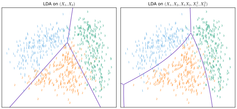
fig_4_1. Reproduces Hastie, Tibshirani and Friedman (2009), Figure 4.1. Download: PDF · SVGSee also (companion courses): Result 4.2 of the Bayesian ML course and Result 5.2 of the deep learning course (convex decision regions).
4.2 Linear Regression of an Indicator Matrix
pp. 103–106 Code the class by \(K\) indicators \(Y_k=\ind\{G=k\}\), collected in the \(N\times K\) indicator matrix \(\bY\) (each row has exactly one 1), and fit all columns at once by least squares:
\[ \hat{\bY}=\X(\X^\T\X)^{-1}\X^\T\bY, \tag{4.3} \]with coefficient matrix \(\hat\bB=(\X^\T\X)^{-1}\X^\T\bY\) of size \((p+1)\times K\). A new \(x\) gets the fitted vector \(\hat f(x)^\T=(1,x^\T)\hat\bB\) and is classified to its largest component,
\[ \hat G(x)=\argmax_{k\in\Gc}\hat f_k(x). \tag{4.4} \]The justification is that \(\E(Y_k\given X=x)=\Pr(G=k\given X=x)\), so each regression estimates a posterior probability, but with a rigid linear form. Equivalently, with targets \(t_k\) (the \(k\)th column of \(\bI_K\)) and \(y_i=t_{g_i}\), fit
\[ \min_{\bB}\sum_{i=1}^N\big\|y_i-[(1,x_i^\T)\bB]^\T\big\|^2 \tag{4.5} \]and classify to the closest target,
\[ \hat G(x)=\argmin_k\|\hat f(x)-t_k\|^2. \tag{4.6} \]Filling the gap 4.1: the fits sum to one, and (4.6) is always (4.4) pp. 104–105
(a) With an intercept, \(\sum_k\hat f_k(x)=1\) for every \(x\) (fitted values may still be negative or above 1). (b) (4.5) is \(K\) separate least squares problems. (c) The closest-target rule (4.6) equals the largest-component rule (4.4) for any vector \(\hat f(x)\), whether or not its components sum to one.
Derivation
(a) Each row of \(\bY\) has a single 1, so \(\bY\mathbf{1}_K=\mathbf{1}_N\). The vector \(\mathbf{1}_N\) is the first column of \(\X\), \(\mathbf{1}_N=\X e_1\), hence \(\hat\bB\mathbf{1}_K=(\X^\T\X)^{-1}\X^\T\X e_1=e_1\) and \(\hat f(x)^\T\mathbf{1}_K=(1,x^\T)e_1=1\). (In the language of the companion course: a linear constraint satisfied by every target is inherited by the prediction, Result 4.3 there.)
(b) \[\sum_i\|y_i-\bB^\T(1,x_i)\|^2=\sum_k\sum_i(y_{ik}-b_k^\T(1,x_i))^2,\] where \(b_k\) is column \(k\) of \(\bB\); the \(k\)th term involves only \(b_k\), so the minimisation splits into one least squares problem per column, whose solutions form (4.3).
(c) Expand \[\|\hat f-t_k\|^2=\|\hat f\|^2-2\hat f_k+\|t_k\|^2=\|\hat f\|^2-2\hat f_k+1.\] Only \(-2\hat f_k\) depends on \(k\), so minimising over \(k\) is maximising \(\hat f_k\). No constraint on \(\sum_k\hat f_k\) is used: the book's remark that the equivalence "does require that the fitted values sum to 1" is not needed (it matters only for coding schemes whose targets have different lengths). Numerically, on the vowel data without an intercept the fitted rows sum to values as far as 0.45 from 1, and the two rules still agree on all 528 points. ∎
See also (companion courses): least squares for classification and the regression function of a 1-of-K target is the posterior.
Masking. With \(K\ge3\) classes the rigid linear fit can make a class never dominate. In Figure 4.2 three well separated classes lie along a diagonal: LDA separates them, while indicator regression gives the middle class a nearly flat fit, so it is almost never the largest. Projecting onto the line through the centroids (Figure 4.3) shows why, and shows that a quadratic regression cures it in this example. The vowel data (Table 4.1, below) give a realistic case: 11 classes in 10 dimensions, where regression has test error 0.67 against 0.56 for LDA.
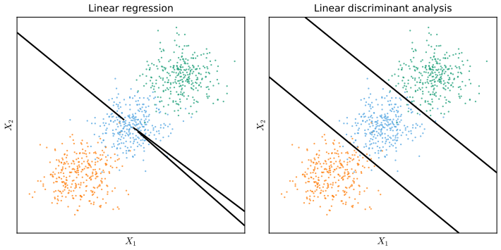
fig_4_2. Reproduces Hastie, Tibshirani and Friedman (2009), Figure 4.2. Download: PDF · SVG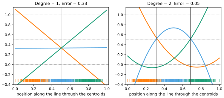
fig_4_3. Reproduces Hastie, Tibshirani and Friedman (2009), Figure 4.3. Download: PDF · SVGFilling the gap 4.2: exactly when a class is masked, and which degree removes it pp. 105–106
Project onto the line through the centroids, coordinate \(t\), and regress the indicators on \(1,t,\dots,t^d\). (a) Degree 1, equal class sizes: every class whose centroid lies strictly between two others is never strictly the largest fit, anywhere on the line. (b) Noiseless limit: if class \(k\) is a point mass at \(t_k\) (equal sizes), the fitted value of class \(k\) at \(t_j\) is the entry \(P_{jk}\) of the hat matrix \(\bP\) of the \(K\times(d+1)\) Vandermonde matrix, so class \(j\) wins at its own location iff \(P_{jj}>P_{jk}\) for all \(k\ne j\). (c) Degree \(K-1\) always suffices (\(\bP=\bI\)), but for equally spaced classes much less is needed: the minimal degree is 2 for \(K=3,4,5\), 3 for \(K=6\)–\(9\), 4 for \(K=10,11\) and 5 for \(K=12\). In particular four lined-up classes are resolved by a quadratic, contrary to the book's remark that a cubic would be needed.
Derivation
(a) With one predictor \(t\), the least squares fit of \(Y_k\) is \(\hat f_k(t)=\bar Y_k+b_k(t-\bar t)\) with \(b_k=\widehat{\cov}(t,Y_k)/\widehat{\var}(t)\). Since \(\bar Y_k=\pi_k:=N_k/N\) and \[\widehat{\cov}(t,Y_k)=\frac1N\sum_i(t_i-\bar t)Y_{ik}=\pi_k(\bar t_k-\bar t),\] where \(\bar t_k\) is the mean of class \(k\),
\[ \hat f_k(t)=\pi_k\Big[1+\frac{(\bar t_k-\bar t)(t-\bar t)}{\widehat{\var}(t)}\Big]. \]With equal \(\pi_k\), at any fixed \(t\) this is an affine function of \(\bar t_k\). An affine function of \(\bar t_k\) over the classes is maximised at the smallest or largest \(\bar t_k\), so a class with \(\bar t_1\lt\bar t_k\lt\bar t_K\) can at best tie (when \(t=\bar t\)) and is never strictly the largest. With three symmetric classes the middle class has \(\bar t_2=\bar t\), so its fit is the constant \(1/3\) (left panel of Figure 4.3).
(b) If the \(N_k=m\) points of class \(k\) all sit at \(t_k\), the model matrix consists of the rows \(v_k^\T=(1,t_k,\dots,t_k^d)\) of the Vandermonde matrix \(\bV_0\), each repeated \(m\) times. Then \(\X^\T\X=m\bV_0^\T\bV_0\) and \(\X^\T\bY e_k=m v_k\), so the fitted value of indicator \(k\) at \(t_j\) is \(v_j^\T(\bV_0^\T\bV_0)^{-1}v_k=P_{jk}\) with \(\bP=\bV_0(\bV_0^\T\bV_0)^{-1}\bV_0^\T\). The points of class \(j\) are correctly classified iff row \(j\) of \(\bP\) has its maximum on the diagonal.
(c) For \(d=K-1\), \(\bV_0\) is square and invertible (distinct \(t_k\)), so \(\bP=\bI\): every class wins at its own location. For \(K=4\) equally spaced points and \(d=2\), \(\bP=\bI-ee^\T/\|e\|^2\) where \(e\perp\{1,t,t^2\}\) is the discrete cubic \(e=(-1,3,-3,1)\), \(\|e\|^2=20\). Row 2 of \(\bP\) is \((0.15,\ 0.55,\ 0.45,\ -0.15)\): the diagonal wins, so no class is masked (and rows 1, 4 have diagonal 0.95). For \(K=5\) and \(d=2\) the margin is thin (row 2 is \((0.257,0.371,0.343,0.086,-0.057)\)), so with noise the inner classes are partly masked: in the demo below, with spacing 4.16 standard deviations, classes 2 and 4 keep only 54% of their points. The minimal degrees quoted in the statement come from checking the condition of (b) for \(d=1,2,\dots\) (masking_min_degree in the code). With 2-D polynomial terms the conclusions are the same, since restricted to points on a line the extra monomials are again polynomials in \(t\) of the same degree.
The book's general heuristic, "polynomial terms up to degree \(K-1\) might be needed", is a safe upper bound by (c); the specific claim about four classes is not correct for equally spaced classes of equal size (a simulation with four classes, sd 1 and spacing 4.16 gives training error 0.041 for the quadratic regression against 0.031 for LDA, and no class loses more than 8% of its points). ∎
See also (companion course): the linear classifiers demo of the Bayesian ML course shows the same three-class masking with Fisher's discriminant and the perceptron.
4.3 Linear Discriminant Analysis
pp. 106–112 By Bayes' theorem, with class densities \(f_k(x)\) and priors \(\pi_k\) (\(\sum_k\pi_k=1\)),
\[ \Pr(G=k\given X=x)=\frac{f_k(x)\pi_k}{\sum_{\ell=1}^Kf_\ell(x)\pi_\ell}. \tag{4.7} \]Gaussian densities give LDA and QDA; mixtures of Gaussians, nonparametric densities and naive Bayes (products of marginals) are other choices (Sections 6.6–6.8 of the book). The multivariate Gaussian density is
\[ f_k(x)=\frac{1}{(2\pi)^{p/2}|\Sigma_k|^{1/2}}\,e^{-\frac12(x-\mu_k)^\T\Sigma_k^{-1}(x-\mu_k)}. \tag{4.8} \]LDA assumes a common covariance \(\Sigma_k=\Sigma\) for all \(k\).
Result 4.2 (Gaussian classes with a common covariance have linear log-odds) pp. 108–109, (4.9)–(4.10)
\[ \log\frac{\Pr(G=k\given X=x)}{\Pr(G=\ell\given X=x)}=\log\frac{\pi_k}{\pi_\ell}-\frac12(\mu_k+\mu_\ell)^\T\Sigma^{-1}(\mu_k-\mu_\ell)+x^\T\Sigma^{-1}(\mu_k-\mu_\ell), \tag{4.9} \]which is linear in \(x\). Equivalently the Bayes rule is \(G(x)=\argmax_k\delta_k(x)\) with the linear discriminant functions
\[ \delta_k(x)=x^\T\Sigma^{-1}\mu_k-\frac12\mu_k^\T\Sigma^{-1}\mu_k+\log\pi_k, \tag{4.10} \]and \(\delta_k(x)-\delta_\ell(x)\) is exactly the log-odds (4.9).
Proof
In the ratio of (4.7) for \(k\) and \(\ell\) the denominators cancel, so the log-odds is \(\log f_k(x)-\log f_\ell(x)+\log(\pi_k/\pi_\ell)\). With a common \(\Sigma\) the normalising constants \((2\pi)^{-p/2}|\Sigma|^{-1/2}\) cancel too, and
\[ -\tfrac12(x-\mu_k)^\T\Sigma^{-1}(x-\mu_k)=-\tfrac12x^\T\Sigma^{-1}x+x^\T\Sigma^{-1}\mu_k-\tfrac12\mu_k^\T\Sigma^{-1}\mu_k \](using the symmetry of \(\Sigma^{-1}\)). The quadratic term \(-\frac12x^\T\Sigma^{-1}x\) is the same for every class and cancels in the difference, leaving \(\delta_k(x)-\delta_\ell(x)\) with \(\delta_k\) as in (4.10). Finally \[\mu_k^\T\Sigma^{-1}\mu_k-\mu_\ell^\T\Sigma^{-1}\mu_\ell=(\mu_k+\mu_\ell)^\T\Sigma^{-1}(\mu_k-\mu_\ell)\] (the cross terms \(\mu_k^\T\Sigma^{-1}\mu_\ell\) cancel by symmetry), which gives (4.9). Because \(\log\) is increasing, the class with the largest posterior is the class with the largest \(\delta_k\). ∎
The boundaries are not the perpendicular bisectors of the segments joining the centroids unless \(\Sigma=\sigma^2\bI\) and the priors are equal: the normal of the \(k\)/\(\ell\) boundary is \(\Sigma^{-1}(\mu_k-\mu_\ell)\). In practice the parameters are replaced by
- \(\hat\pi_k=N_k/N\);
- \(\hat\mu_k=\sum_{g_i=k}x_i/N_k\);
- \[\hat\Sigma=\sum_{k=1}^K\sum_{g_i=k}(x_i-\hat\mu_k)(x_i-\hat\mu_k)^\T/(N-K).\]
Filling the gap 4.3: where these estimates come from p. 109
\(\hat\pi_k\) and \(\hat\mu_k\) maximise the joint likelihood of \((x_i,g_i)\) under the model \(\Pr(G=k)=\pi_k\), \(X\given G=k\sim\N(\mu_k,\Sigma)\); the maximum likelihood covariance is the same sum divided by \(N\), and dividing by \(N-K\) makes it unbiased.
Derivation
The log-likelihood is \[\sum_i\log\pi_{g_i}+\sum_i\log\phi(x_i;\mu_{g_i},\Sigma)=\sum_kN_k\log\pi_k-\frac N2\log|\Sigma|-\frac12\sum_i(x_i-\mu_{g_i})^\T\Sigma^{-1}(x_i-\mu_{g_i})+\text{const}.\] The first part is maximised subject to \(\sum_k\pi_k=1\) by a Lagrange multiplier: \(N_k/\pi_k=\lambda\), so \(\pi_k\propto N_k\), \(\hat\pi_k=N_k/N\). For each \(k\) the terms with \(g_i=k\) are a quadratic in \(\mu_k\) minimised at the class mean. Writing \(\mathbf{S}=\sum_i(x_i-\hat\mu_{g_i})(x_i-\hat\mu_{g_i})^\T\), the profile log-likelihood in \(\mathbf{\Omega}=\Sigma^{-1}\) is \(\frac N2\log|\mathbf{\Omega}|-\frac12\Tr(\mathbf{\Omega}\mathbf{S})\), with gradient \(\frac N2\mathbf{\Omega}^{-1}-\frac12\mathbf{S}\) (matrix calculus), zero at \(\Sigma=\mathbf{S}/N\). For unbiasedness: within class \(k\), \[\E\sum_{g_i=k}(x_i-\hat\mu_k)(x_i-\hat\mu_k)^\T=(N_k-1)\Sigma\] (the usual sample covariance argument), and summing over classes gives \((N-K)\Sigma\). Changing the divisor multiplies \(\hat\Sigma\) by a constant: this rescales the \(x\)-dependent part of every \(\delta_k\) by the same factor but not the \(\log\hat\pi_k\) terms, so it can change a classification only when the priors differ, and then rarely. ∎
See also (companion courses): Result 4.9 and Result 4.10 of the Bayesian ML course; Result 5.11 and Result 5.12 of the deep learning course, with the generative classifier demo.
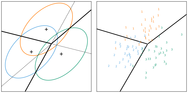
fig_4_5. Reproduces Hastie, Tibshirani and Friedman (2009), Figure 4.5. Download: PDF · SVGTwo classes. The LDA rule classifies to class 2 if
\[ x^\T\hat\Sigma^{-1}(\hat\mu_2-\hat\mu_1)>\frac12\hat\mu_2^\T\hat\Sigma^{-1}\hat\mu_2-\frac12\hat\mu_1^\T\hat\Sigma^{-1}\hat\mu_1+\log(N_1/N)-\log(N_2/N). \tag{4.11} \]Result 4.3 (two classes: least squares finds the LDA direction but not its cut-point; Exercise 4.2) pp. 109–110
Regress any two-valued coding of the classes on \(x\) by least squares. The coefficient vector is a positive (for the coding \(-N/N_1,\,N/N_2\)) multiple of \(\hat\Sigma^{-1}(\hat\mu_2-\hat\mu_1)\). With \(\Delta^2=(\hat\mu_2-\hat\mu_1)^\T\hat\Sigma^{-1}(\hat\mu_2-\hat\mu_1)\), the rule "class 2 if the fit is positive" and the LDA rule (4.11) use the same direction with thresholds that differ by
\[ \frac{(N_2-N_1)\Delta^2}{2N}-\log\frac{N_1}{N_2}, \]which is zero iff \(N_1=N_2\) (for \(\Delta>0\)). Proof: Exercise 4.2.
The direction does not need Gaussian data; the cut-point in (4.11) does, so the book suggests choosing the cut-point to minimise the training error. With more than two classes LDA and indicator regression differ, and LDA avoids masking; the link between them is optimal scoring (Section 12.5 of the book; see also Exercise 4.3).
See also (companion course): Result 4.5 of the Bayesian ML course (Fisher's discriminant as least squares).
Quadratic discriminant analysis. Without a common covariance the quadratic terms no longer cancel:
\[ \delta_k(x)=-\frac12\log|\Sigma_k|-\frac12(x-\mu_k)^\T\Sigma_k^{-1}(x-\mu_k)+\log\pi_k. \tag{4.12} \]Filling the gap 4.4: QDA, and counting parameters pp. 110–111
(4.12) is \(\log f_k(x)\pi_k\) without the constant \(-\frac p2\log2\pi\), so \(\argmax_k\delta_k\) is the Bayes rule; the boundaries \(\{\delta_k=\delta_\ell\}\) are quadrics. LDA's decision rule depends on \((K-1)(p+1)\) numbers and QDA's on \((K-1)\{p(p+3)/2+1\}\).
Derivation
Take logs in (4.8) and add \(\log\pi_k\); dropping the class-independent constant gives (4.12). \(\delta_k-\delta_\ell\) is \(-\frac12x^\T(\Sigma_k^{-1}-\Sigma_\ell^{-1})x\) plus linear and constant terms: a quadric unless \(\Sigma_k=\Sigma_\ell\).
The classification depends only on the \(K-1\) differences \(\delta_k-\delta_K\), since adding a common function to all \(\delta_k\) does not change the argmax. For LDA each difference is affine in \(x\): \(p\) slopes and an intercept, \((K-1)(p+1)\) in all (the \(p(p+1)/2\) entries of \(\hat\Sigma\) are used only through these combinations, the book's footnote 3). For QDA each difference is a general quadratic: a symmetric matrix (\(p(p+1)/2\) entries), \(p\) linear coefficients and a constant, \(p(p+1)/2+p+1=p(p+3)/2+1\) numbers. For the vowel data (\(p=10\), \(K=11\)) that is 110 against 660. ∎
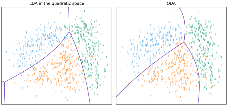
fig_4_6. Reproduces Hastie, Tibshirani and Friedman (2009), Figure 4.6. Download: PDF · SVGSee also (companion course): Filling the gap 5.8 of the deep learning course (different covariances give quadratic boundaries).
LDA and QDA do well on many problems (the STATLOG comparison of Michie et al., 1994). The book's explanation is a bias–variance one: data can often support only simple boundaries, and the Gaussian plug-in estimates of linear or quadratic boundaries are stable.
The vowel data. 11 vowel sounds spoken by different speakers, each represented by \(p=10\) features; 528 training vectors (48 per class) and 462 test vectors. Table 4.1 is reproduced exactly:
| Technique (Table 4.1) | Training error | Test error | book |
|---|---|---|---|
| Linear regression | 0.4773 | 0.6667 | 0.48 / 0.67 |
| Linear discriminant analysis | 0.3163 | 0.5563 | 0.32 / 0.56 |
| Quadratic discriminant analysis | 0.0114 | 0.5281 | 0.01 / 0.53 |
| Logistic regression (multinomial, Exercise 4.4) | 0.2235 | 0.5130 | 0.22 / 0.51 |
Code: vowel_errors (printed by fig_4_4).
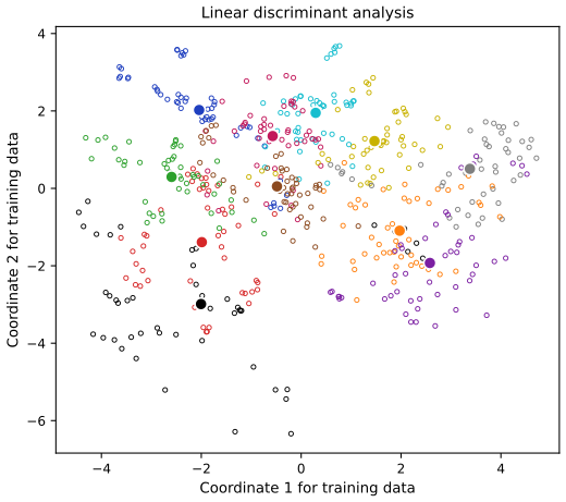
fig_4_4. Reproduces Hastie, Tibshirani and Friedman (2009), Figure 4.4. Download: PDF · SVG4.3.1 Regularized Discriminant Analysis
pp. 112–113 Friedman (1989) shrinks the class covariances of QDA towards the pooled one,
\[ \hat\Sigma_k(\alpha)=\alpha\hat\Sigma_k+(1-\alpha)\hat\Sigma, \tag{4.13} \]\(\alpha\in[0,1]\) running from LDA (\(\alpha=0\)) to QDA (\(\alpha=1\)), and similarly shrinks \(\hat\Sigma\) towards a multiple of the identity,
\[ \hat\Sigma(\gamma)=\gamma\hat\Sigma+(1-\gamma)\hat\sigma^2\bI. \tag{4.14} \]Filling the gap 4.5: what the two shrinkages do p. 112
(a) If \(\hat\Sigma\) is positive definite, \(\hat\Sigma_k(\alpha)\) is positive definite for every \(\alpha\lt1\), even when \(N_k\le p\) makes \(\hat\Sigma_k\) singular. (b) With \(\hat\sigma^2=\Tr(\hat\Sigma)/p\) (the natural choice, used in the code), \(\hat\Sigma(\gamma)\) has the same eigenvectors as \(\hat\Sigma\) and eigenvalues \(\gamma d_j+(1-\gamma)\bar d\), pulled towards their mean \(\bar d\): its condition number decreases as \(\gamma\) decreases, and \(\Tr\hat\Sigma(\gamma)=\Tr\hat\Sigma\). This is the analogue of ridge regression, which adds \(\lambda\bI\) to \(\X^\T\X\).
Derivation
(a) For \(v\ne0\), \[v^\T\hat\Sigma_k(\alpha)v=\alpha v^\T\hat\Sigma_kv+(1-\alpha)v^\T\hat\Sigma v\ge(1-\alpha)v^\T\hat\Sigma v>0.\] (b) With \(\hat\Sigma=\bU\bD\bU^\T\), \(\hat\Sigma(\gamma)=\bU(\gamma\bD+(1-\gamma)\bar d\bI)\bU^\T\) because \(\bU\bU^\T=\bI\). The ratio of largest to smallest eigenvalue, \((\gamma d_1+(1-\gamma)\bar d)/(\gamma d_p+(1-\gamma)\bar d)\), is increasing in \(\gamma\) when \(d_1>d_p\) (its derivative has the sign of \((d_1-d_p)\bar d>0\)). The trace is \(\gamma\sum d_j+(1-\gamma)p\bar d=\sum d_j\). Inverting a covariance multiplies the variance in each eigendirection by its reciprocal, so small, poorly estimated eigenvalues dominate \(\hat\Sigma^{-1}\); shrinking them towards the mean reduces the variance of the discriminant functions at the cost of bias. ∎
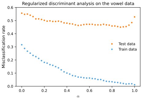
fig_4_7. Reproduces Hastie, Tibshirani and Friedman (2009), Figure 4.7. Download: PDF · SVGThe large gap between training and test error is partly a property of the data: the training and test sets come from different speakers, each repeating every vowel several times.
4.3.2 Computations for LDA
p. 113 Diagonalise: \(\hat\Sigma_k=\bU_k\bD_k\bU_k^\T\) with \(\bU_k\) orthogonal and \(\bD_k\) diagonal with entries \(d_{k\ell}>0\). Then the ingredients of (4.12) are \[(x-\hat\mu_k)^\T\hat\Sigma_k^{-1}(x-\hat\mu_k)=[\bU_k^\T(x-\hat\mu_k)]^\T\bD_k^{-1}[\bU_k^\T(x-\hat\mu_k)]\] and \(\log|\hat\Sigma_k|=\sum_\ell\log d_{k\ell}\).
Result 4.4 (LDA is nearest-centroid classification after sphering) p. 113
Let \(\hat\Sigma=\bU\bD\bU^\T\) and \(x^*=\bD^{-1/2}\bU^\T x\). Then the within-class covariance of the \(x^*\) is \(\bI\), and
\[ \delta_k(x)=-\tfrac12\|x^*-\hat\mu_k^*\|^2+\log\hat\pi_k+c(x), \]where \(c(x)\) does not depend on \(k\). So LDA classifies to the closest centroid in the sphered space, after correcting the squared distance by \(-2\log\hat\pi_k\).
Proof
\[\cov(x^*)=\bD^{-1/2}\bU^\T\hat\Sigma\bU\bD^{-1/2}=\bD^{-1/2}\bD\bD^{-1/2}=\bI.\] Since \[\hat\Sigma^{-1}=\bU\bD^{-1}\bU^\T=(\bD^{-1/2}\bU^\T)^\T(\bD^{-1/2}\bU^\T),\] we have \((x-\mu)^\T\hat\Sigma^{-1}(x-\mu)=\|x^*-\mu^*\|^2\). Expanding as in Result 4.2, \[-\frac12\|x^*-\hat\mu_k^*\|^2=-\frac12\|x^*\|^2+x^\T\hat\Sigma^{-1}\hat\mu_k-\frac12\hat\mu_k^\T\hat\Sigma^{-1}\hat\mu_k,\] which is \(\delta_k(x)-\log\hat\pi_k\) plus \(-\frac12\|x^*\|^2\). On the vowel data the two computations give the same class for every test vector. ∎
4.3.3 Reduced-Rank Linear Discriminant Analysis
pp. 113–119 LDA also gives informative low-dimensional views of the data.
Result 4.5 (LDA lives in a space of dimension at most \(K-1\)) pp. 113–114
In the sphered space the \(K\) centroids lie in an affine subspace \(H_{K-1}\) of dimension \(r\le\min(K-1,p)\). If \(\bP\) is the orthogonal projection onto the directions of \(H_{K-1}\) (the span of \(\hat\mu_k^*-\hat\mu_1^*\)), then \[\|x^*-\hat\mu_k^*\|^2=\|\bP(x^*-\hat\mu_k^*)\|^2+\|(\bI-\bP)(x^*-\hat\mu_1^*)\|^2,\] and the second term does not depend on \(k\). Hence LDA uses only the projection of \(x^*\) onto \(H_{K-1}\).
Proof
\(K\) points span an affine set of dimension at most \(K-1\) (the differences \(\hat\mu_k^*-\hat\mu_1^*\), \(k=2,\dots,K\), are \(K-1\) vectors in \(\R^p\)). Write \(x^*-\hat\mu_k^*=(x^*-\hat\mu_1^*)-(\hat\mu_k^*-\hat\mu_1^*)\). The second vector is in the range of \(\bP\), so \[(\bI-\bP)(x^*-\hat\mu_k^*)=(\bI-\bP)(x^*-\hat\mu_1^*)\] for every \(k\), and Pythagoras splits the squared norm into the two orthogonal parts. ∎
For \(K>3\) one can ask for the best \(L\)-dimensional subspace \(H_L\subseteq H_{K-1}\). Fisher's criterion: spread the projected centroids as much as possible (principal components of the sphered centroids). The recipe is
- compute the \(K\times p\) matrix of class centroids \(\bM\) and the within-class covariance \(\bW\);
- compute \(\bM^*=\bM\bW^{-1/2}\) using the eigen-decomposition of \(\bW\);
- compute \(\bB^*\), the covariance of the rows of \(\bM^*\), and its eigen-decomposition \(\bB^*=\bV^*\bD_B\bV^{*\T}\); the columns \(v_\ell^*\), in order, define the optimal subspaces,
and the \(\ell\)th discriminant variable is \(Z_\ell=v_\ell^\T X\) with \(v_\ell=\bW^{-1/2}v_\ell^*\). Fisher's own formulation: find \(Z=a^\T X\) maximising the ratio of between-class to within-class variance, the Rayleigh quotient
\[ \max_a\frac{a^\T\bB a}{a^\T\bW a}, \tag{4.15} \] \[ \max_a a^\T\bB a\ \ \text{subject to}\ \ a^\T\bW a=1. \tag{4.16} \]Result 4.6 (Fisher's problem is a generalised eigenproblem whose solutions are the discriminant coordinates; Exercise 4.1) pp. 114–116
Let \(\bW\) be positive definite and \(\bB\) positive semidefinite. (a) The maximum of (4.15) is the largest eigenvalue \(\lambda_1\) of \(\bW^{-1}\bB\) (equivalently of \(\bB^*=\bW^{-1/2}\bB\bW^{-1/2}\)), attained at \(a_1=\bW^{-1/2}v_1^*=v_1\). (b) Among directions with \(a^\T\bW a_j=0\) for \(j\lt\ell\), the maximum is \(\lambda_\ell\), attained at \(a_\ell=v_\ell\). (c) The coordinates \(Z_\ell=v_\ell^\T X\) are uncorrelated within classes with unit within-class variance (\(v_\ell^\T\bW v_m=\delta_{\ell m}\)), and their class means are uncorrelated with between-class variances \(\lambda_\ell\) (\(v_\ell^\T\bB v_m=\lambda_\ell\delta_{\ell m}\)). (d) Classifying to the nearest centroid using \(Z_1,\dots,Z_L\) with \(L=\rank\bB\) is LDA.
Proof
Substitute \(b=\bW^{1/2}a\), a bijection of \(\R^p\setminus\{0\}\). Then \(a^\T\bB a/a^\T\bW a=b^\T\bB^*b/b^\T b\), a Rayleigh quotient of the symmetric matrix \(\bB^*\). Expanding \(b=\sum_jc_jv_j^*\) in its orthonormal eigenvectors gives \(b^\T\bB^*b/b^\T b=\sum_j\lambda_jc_j^2/\sum_jc_j^2\le\lambda_1\), with equality at \(b=v_1^*\), i.e. \(a=\bW^{-1/2}v_1^*\) (Rayleigh quotients in the toolkit). This proves (a); the stationarity condition \(\bB a=\lambda\bW a\) is the generalised eigenproblem, and \(\bW^{-1}\bB a=\lambda a\) has the same eigenvalues as \(\bB^*\) (similar matrices: \(\bW^{-1}\bB=\bW^{-1/2}\bB^*\bW^{1/2}\)). (b) \(a^\T\bW a_j=b^\T v_j^*\), so the constraint says \(c_j=0\) for \(j\lt\ell\); the same expansion gives the bound \(\lambda_\ell\), attained at \(v_\ell^*\). (c) \(v_\ell^\T\bW v_m=v_\ell^{*\T}v_m^*=\delta_{\ell m}\) and \(v_\ell^\T\bB v_m=v_\ell^{*\T}\bB^*v_m^*=\lambda_m\delta_{\ell m}\). (d) The \(v_\ell^*\) with \(\lambda_\ell>0\) span the range of \(\bB^*\), which is the span of the centred sphered centroids, i.e. the directions of \(H_{K-1}\); by Result 4.5 the nearest-centroid computation needs nothing else. The three-step recipe above and the generalised eigenproblem therefore give the same directions (numerically: the eigenvalues agree with those of scipy.linalg.eigh(B, W) to \(10^{-9}\), and the first two coordinates span the same plane as scikit-learn's). ∎
See also (companion course): Result 4.4 (Fisher, two classes) and Result 4.6 (the multiclass criterion) of the Bayesian ML course.
Filling the gap 4.6: \(\bB+\bW=\bT\) needs matching conventions p. 114
Let \(\bT=\frac1N\sum_i(x_i-\bar x)(x_i-\bar x)^\T\), \(\bW_N=\frac1N\sum_i(x_i-\hat\mu_{g_i})(x_i-\hat\mu_{g_i})^\T\) and \(\bB_\pi=\sum_k\hat\pi_k(\hat\mu_k-\bar x)(\hat\mu_k-\bar x)^\T\). Then \(\bT=\bW_N+\bB_\pi\) exactly. With other divisors (\(N-K\) for \(\bW\), or the unweighted covariance of the \(K\) centroids for \(\bB\)) the identity holds only approximately. The discriminant directions do not depend on these conventions when the classes have equal sizes (as for the vowel data), and positive rescalings of \(\bB\) or \(\bW\) only rescale the eigenvalues.
Derivation
Write \(x_i-\bar x=(x_i-\hat\mu_{g_i})+(\hat\mu_{g_i}-\bar x)\) and expand the outer product. The cross terms vanish after summing within each class, since \(\sum_{g_i=k}(x_i-\hat\mu_k)=0\). The remaining terms give \(N\bW_N\) and \(\sum_kN_k(\hat\mu_k-\bar x)(\hat\mu_k-\bar x)^\T=N\bB_\pi\). If the \(N_k\) differ, weighting the centroids equally changes \(\bB\) and hence the directions; the weighted version is the one that arises from maximum likelihood (Exercise 4.8). Replacing \(\bW\) by \(c\bW\) or \(\bB\) by \(c\bB\) (\(c>0\)) multiplies (4.15) by a constant and leaves its maximisers unchanged. ∎
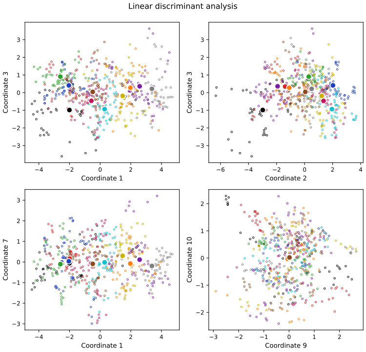
fig_4_8. Reproduces Hastie, Tibshirani and Friedman (2009), Figure 4.8. Download: PDF · SVGFigure 4.9 shows why the within-class covariance matters: the line joining the centroids separates the means most, but the projected classes overlap because of the covariance.
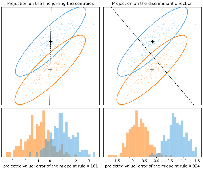
fig_4_9. Reproduces Hastie, Tibshirani and Friedman (2009), Figure 4.9. Download: PDF · SVGFilling the gap 4.7: the error of a projection, and the role of \(\log\pi_k\) pp. 116–117
For two classes \(\N(\mu_k,\Sigma)\) and a direction \(a\), the projections are \(\N(a^\T\mu_k,\,a^\T\Sigma a)\). With equal priors the best cut-point on the projection is the midpoint, with error \(\Phi(-\delta(a)/2)\), where \(\delta(a)=|a^\T(\mu_2-\mu_1)|/\sqrt{a^\T\Sigma a}\). This is maximised by \(a\propto\Sigma^{-1}(\mu_2-\mu_1)\), where \(\delta\) equals the Mahalanobis distance \(\Delta\). With unequal priors the optimal cut moves towards the smaller class by \(\log(\pi_1/\pi_2)/\Delta\) standard deviations.
Derivation
Standardise the projection by \(s=\sqrt{a^\T\Sigma a}\); the two classes become \(\N(m_1,1)\) and \(\N(m_2,1)\) with \(|m_2-m_1|=\delta\). The posterior log-odds is linear, \(\log(\pi_2/\pi_1)+\delta(u-\frac{m_1+m_2}2)\) (for \(m_2>m_1\)), so the Bayes cut is \(u_0=\frac{m_1+m_2}2+\log(\pi_1/\pi_2)/\delta\); for equal priors it is the midpoint and the error is \(\frac12\Phi(-\delta/2)+\frac12\Phi(-\delta/2)\). By Cauchy–Schwarz in the inner product \(\langle u,v\rangle=u^\T\Sigma v\), \[|a^\T d|=|\langle a,\Sigma^{-1}d\rangle|\le\sqrt{a^\T\Sigma a}\sqrt{d^\T\Sigma^{-1}d}\] with \(d=\mu_2-\mu_1\), so \(\delta(a)\le\Delta\), with equality iff \(a\propto\Sigma^{-1}d\). The error \(\Phi(-\delta/2)\) is decreasing in \(\delta\), so this direction is optimal for every Gaussian two-class problem with a common covariance. ∎
Reduced subspaces can also be used for classification: compute distances to the centroids only in the first \(L\) coordinates. This is the Bayes rule of a Gaussian model whose centroids are restricted to an \(L\)-dimensional subspace:
Result 4.7 (reduced-rank LDA is constrained maximum likelihood; Exercise 4.8) p. 117
Fit \(X\given G=k\sim\N(\mu_k,\Sigma)\) by maximum likelihood subject to: the centroids lie in an affine subspace of dimension \(L\). Then \(\hat\Sigma=\bW_N^{1/2}\{\bI+\sum_{\ell>L}\lambda_\ell v_\ell^*v_\ell^{*\T}\}\bW_N^{1/2}\) and the fitted centroids are the projections of the \(\hat\mu_k\) onto the first \(L\) discriminant coordinates; the Bayes rule of the fitted model is to classify to the nearest centroid in the first \(L\) discriminant coordinates (corrected by \(\log\hat\pi_k\)), i.e. reduced-rank LDA. Proof: Exercise 4.8.
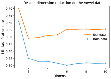
fig_4_10. Reproduces Hastie, Tibshirani and Friedman (2009), Figure 4.10. Download: PDF · SVG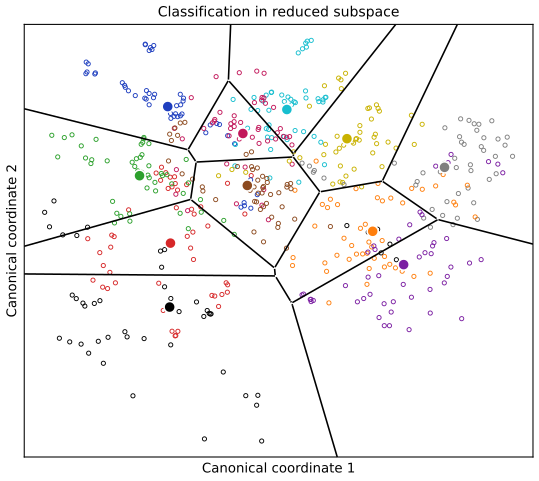
fig_4_11. Reproduces Hastie, Tibshirani and Friedman (2009), Figure 4.11. Download: PDF · SVGThe connection with indicator regression: LDA can be computed by regressing \(\bY\) on \(\X\) and then eigen-decomposing \(\hat\bY^\T\bY\) (Section 12.5 of the book), and LDA on the fitted values \(\hat\bY\) is the same as LDA on \(X\) (Exercise 4.3).
4.4 Logistic Regression
pp. 119–120 Model the \(K-1\) log-odds against a reference class (the last) as linear functions:
\[ \log\frac{\Pr(G=k\given X=x)}{\Pr(G=K\given X=x)}=\beta_{k0}+\beta_k^\T x,\qquad k=1,\dots,K-1. \tag{4.17} \]Solving for the probabilities gives
\[ \Pr(G=k\given X=x)=\frac{\exp(\beta_{k0}+\beta_k^\T x)}{1+\sum_{\ell=1}^{K-1}\exp(\beta_{\ell0}+\beta_\ell^\T x)},\ \ k\lt K,\qquad \Pr(G=K\given X=x)=\frac{1}{1+\sum_{\ell=1}^{K-1}\exp(\beta_{\ell0}+\beta_\ell^\T x)}, \tag{4.18} \]written \(p_k(x;\theta)\), with \(\theta=\{\beta_{10},\beta_1^\T,\dots,\beta_{(K-1)0},\beta_{K-1}^\T\}\).
Filling the gap 4.8: from (4.17) to (4.18), and why the reference class does not matter p. 119
Derivation
Write \(\eta_k=\beta_{k0}+\beta_k^\T x\) and \(p_k=\Pr(G=k\given X=x)\). (4.17) says \(p_k=p_Ke^{\eta_k}\) for \(k\lt K\). Summing over all classes, \(1=p_K(1+\sum_{\ell\lt K}e^{\eta_\ell})\), which gives \(p_K\) and then each \(p_k\): (4.18). The probabilities are positive and sum to one by construction. If instead class \(j\) is the reference, the log-odds against \(j\) are \(\log(p_k/p_j)=\eta_k-\eta_j\) (with \(\eta_K=0\)), again linear in \(x\): the reparametrisation \(\beta'_k=\beta_k-\beta_j\) is a bijection between the two parameter sets that leaves every probability unchanged. Maximum likelihood estimates therefore transform in the same way (they are equivariant), and fitted probabilities do not depend on the choice. ∎
4.4.1 Fitting Logistic Regression Models
pp. 120–122 The fit maximises the conditional log-likelihood
\[ \ell(\theta)=\sum_{i=1}^N\log p_{g_i}(x_i;\theta). \tag{4.19} \]For two classes code \(y_i=1\) if \(g_i=1\) and \(0\) otherwise, let \(p(x;\beta)=p_1(x;\theta)\), and let \(x_i\) include the constant 1. Then
\[ \ell(\beta)=\sum_{i=1}^N\big\{y_i\log p(x_i;\beta)+(1-y_i)\log(1-p(x_i;\beta))\big\}=\sum_{i=1}^N\big\{y_i\beta^\T x_i-\log(1+e^{\beta^\T x_i})\big\}. \tag{4.20} \]Result 4.8 (score, Hessian, concavity, and Newton–Raphson as IRLS) pp. 120–121, (4.21)–(4.28)
The score and the Hessian of (4.20) are
\[ \frac{\partial\ell(\beta)}{\partial\beta}=\sum_{i=1}^Nx_i(y_i-p(x_i;\beta)), \tag{4.21} \] \[ \frac{\partial^2\ell(\beta)}{\partial\beta\partial\beta^\T}=-\sum_{i=1}^Nx_ix_i^\T p(x_i;\beta)(1-p(x_i;\beta)), \tag{4.22} \]so \(\ell\) is concave, strictly if \(\X\) has full column rank. A Newton step from \(\beta^{\rm old}\) is
\[ \beta^{\rm new}=\beta^{\rm old}-\Big(\frac{\partial^2\ell(\beta)}{\partial\beta\partial\beta^\T}\Big)^{-1}\frac{\partial\ell(\beta)}{\partial\beta}. \tag{4.23} \]In matrix form, with \(\bp\) the fitted probabilities at \(\beta^{\rm old}\) and \(\bW=\diag\{p_i(1-p_i)\}\),
\[ \frac{\partial\ell(\beta)}{\partial\beta}=\X^\T(\y-\bp), \tag{4.24} \] \[ \frac{\partial^2\ell(\beta)}{\partial\beta\partial\beta^\T}=-\X^\T\bW\X, \tag{4.25} \] \[ \beta^{\rm new}=\beta^{\rm old}+(\X^\T\bW\X)^{-1}\X^\T(\y-\bp)=(\X^\T\bW\X)^{-1}\X^\T\bW\big(\X\beta^{\rm old}+\bW^{-1}(\y-\bp)\big)=(\X^\T\bW\X)^{-1}\X^\T\bW\bz, \tag{4.26} \] \[ \bz=\X\beta^{\rm old}+\bW^{-1}(\y-\bp), \tag{4.27} \] \[ \beta^{\rm new}\leftarrow\argmin_\beta(\bz-\X\beta)^\T\bW(\bz-\X\beta). \tag{4.28} \]Each Newton step is a weighted least squares fit of the adjusted response \(\bz\): iteratively reweighted least squares (IRLS).
Proof
\(\frac{\d}{\d\eta}\log(1+e^\eta)=\frac{e^\eta}{1+e^\eta}=\sigma(\eta)\) and \(\sigma'(\eta)=\sigma(\eta)(1-\sigma(\eta))\). With \(\eta_i=\beta^\T x_i\), the chain rule gives \[\partial_\beta\{y_i\eta_i-\log(1+e^{\eta_i})\}=x_i(y_i-p_i),\] which is (4.21), and differentiating \(-x_ip_i\) once more gives \(-x_ix_i^\T p_i(1-p_i)\), (4.22). Stacking: \(\sum_ix_i(y_i-p_i)=\X^\T(\y-\bp)\) and \(\sum_ix_ix_i^\T w_i=\X^\T\bW\X\). For any \(v\), \(v^\T\X^\T\bW\X v=\sum_iw_i(x_i^\T v)^2\ge0\) because \(0\lt w_i\le\frac14\); it vanishes only if \(\X v=0\), so with full column rank the Hessian is negative definite and \(\ell\) strictly concave. (4.26): insert \(\X^\T\bW\X\beta^{\rm old}\) and factor \(\X^\T\bW\): \[\X^\T\bW\X\beta^{\rm old}+\X^\T(\y-\bp)=\X^\T\bW(\X\beta^{\rm old}+\bW^{-1}(\y-\bp)).\] (4.28) is the weighted normal equations \(\X^\T\bW\X\beta=\X^\T\bW\bz\). On the heart disease data the Hessian formula agrees with finite differences of the score, and the Newton and weighted least squares steps agree to \(10^{-9}\). ∎
See also (companion courses): Result 4.12, Result 4.14 and Filling the gap 4.6 of the Bayesian ML course (the same derivation in Bishop's notation); Result 5.16 of the deep learning course.
Filling the gap 4.9: starting values, step halving and convergence p. 121
(a) From \(\beta=0\) the first IRLS step is an ordinary least squares regression: all \(p_i=\frac12\), \(\bW=\frac14\bI\), \(\bz=4(\y-\frac12)\), so \(\beta^{(1)}=4\hat b-2e_1\), where \(\hat b\) is the least squares fit of \(\y\) on \(\X\). (b) The Newton direction is an ascent direction, so halving the step until \(\ell\) increases always succeeds; if the maximiser exists (no separation, full rank), the damped iteration converges to it, and near it the convergence is quadratic. (c) If the classes are separable by a hyperplane, \(\ell\lt0\) can be pushed arbitrarily close to 0 and there is no maximiser (Exercise 4.5); the iterates diverge.
Derivation
(a) Substitute in (4.26): \[\beta^{(1)}=(\frac14\X^\T\X)^{-1}\frac14\X^\T\cdot4(\y-\frac12\mathbf1)=4(\X^\T\X)^{-1}\X^\T\y-2(\X^\T\X)^{-1}\X^\T\X e_1.\] So the first step already points in the least squares (for two classes: the LDA) direction (Result 4.3). On the heart disease data the deviance \(-2\ell\) goes 640.47, 491.59, 483.40, 483.17433, 483.17403 and stays there: five steps to convergence.
(b) Let \(g=\nabla\ell(\beta)\ne0\) and \(d=(\X^\T\bW\X)^{-1}g\). Then \(g^\T d>0\) because \((\X^\T\bW\X)^{-1}\) is positive definite, so \[\ell(\beta+td)=\ell(\beta)+tg^\T d+o(t)>\ell(\beta)\] for small \(t>0\): halving finds such \(t\) after finitely many trials. Each accepted step increases \(\ell\); when the maximiser exists the upper level sets of the strictly concave \(\ell\) are compact, and the standard theory of damped Newton methods for strictly concave smooth functions (e.g. Boyd and Vandenberghe 2004, Section 9.5) gives convergence, with full steps and quadratic convergence eventually. The book's "convergence is never guaranteed" refers to undamped steps, which can overshoot. (c) is Exercise 4.5. ∎
For \(K\ge3\) Newton's method has the same form with a vector of \(K-1\) responses per observation and a non-diagonal \((K-1)\times(K-1)\) weight block per observation (Exercise 4.4); coordinate descent (as in glmnet; Friedman et al., 2010) is an alternative for large problems. Applied to the vowel data, it gives the logistic regression row of Table 4.1.
See also (companion courses): Result 4.15 of the Bayesian ML course and Result 5.18 of the deep learning course (softmax derivatives).
4.4.2 Example: South African Heart Disease
pp. 122–124 462 white males aged 15–64 from a heart disease risk-factor study in the Western Cape (Rousseauw et al., 1983): 160 cases of myocardial infarction and 302 controls. Figure 4.12 shows the risk factors.
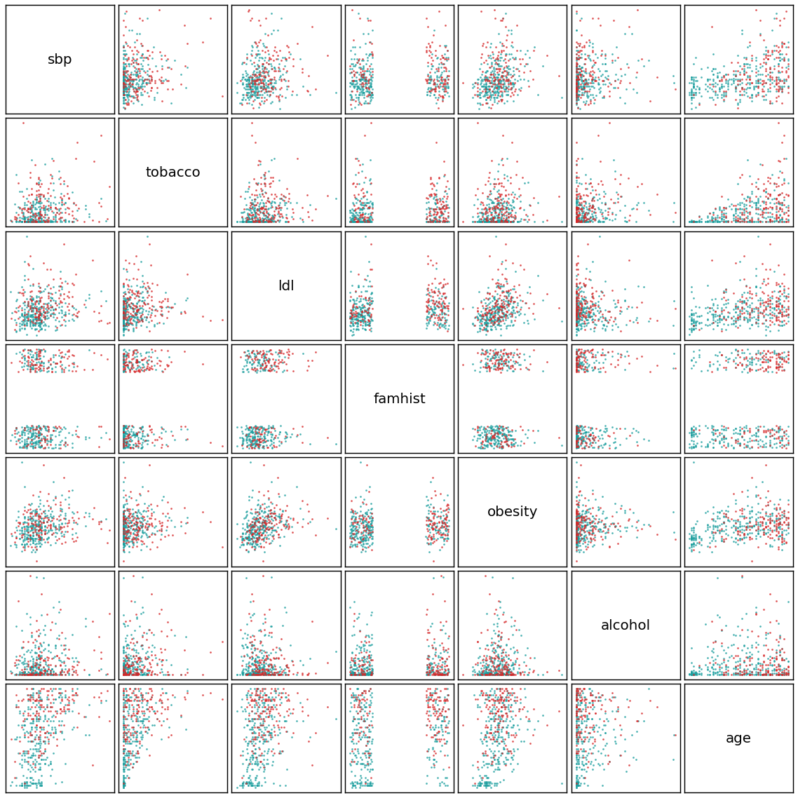
fig_4_12. Reproduces Hastie, Tibshirani and Friedman (2009), Figure 4.12. Download: PDF · PNGThe maximum likelihood fit (Table 4.2) and the model after backward elimination (Table 4.3), reproduced:
| Table 4.2 | Coefficient | Std. error | Z score | book Z |
|---|---|---|---|---|
| (Intercept) | −4.130 | 0.964 | −4.283 | −4.285 |
| sbp | 0.006 | 0.006 | 1.023 | 1.023 |
| tobacco | 0.080 | 0.026 | 3.034 | 3.034 |
| ldl | 0.185 | 0.057 | 3.218 | 3.219 |
| famhist | 0.939 | 0.225 | 4.177 | 4.178 |
| obesity | −0.035 | 0.029 | −1.187 | −1.187 |
| alcohol | 0.001 | 0.004 | 0.136 | 0.136 |
| age | 0.043 | 0.010 | 4.181 | 4.184 |
| Table 4.3 | Coefficient | Std. error | Z score | book Z |
|---|---|---|---|---|
| (Intercept) | −4.204 | 0.498 | −8.44 | −8.45 |
| tobacco | 0.081 | 0.026 | 3.16 | 3.16 |
| ldl | 0.168 | 0.054 | 3.09 | 3.09 |
| famhist | 0.924 | 0.223 | 4.14 | 4.14 |
| age | 0.044 | 0.010 | 4.52 | 4.52 |
All coefficients and standard errors agree with the book to the three decimals printed; four Z scores differ in the third decimal (at most 0.003), and the intercept Z of Table 4.3 is \(-4.2043/0.4983=-8.44\), not \(-8.45\). Code: saheart_tables (printed by fig_4_13). The residual deviances are 483.174 (seven inputs) and 485.444 (four).
Filling the gap 4.10: Z scores, odds ratios and the analysis of deviance pp. 122–124
(a) The Z score \(\hat\beta_j/\widehat{\rm se}_j\), with \(\widehat{\rm se}_j^2=[(\X^\T\hat\bW\X)^{-1}]_{jj}\), is the Wald statistic for \(H_0:\beta_j=0\) given the other terms, approximately \(\N(0,1)\) under \(H_0\) (Result 4.9); \(|Z|>1.96\) is significance at 5%. (b) \(e^{\beta_j}\) is the factor by which the odds of disease are multiplied when \(x_j\) increases by one unit, the others fixed; an approximate 95% interval is \(\exp(\hat\beta_j\pm2\widehat{\rm se}_j)\). (c) For nested models \(M_0\subset M_1\) differing by \(q\) parameters, the change in residual deviance \(\Dev_0-\Dev_1=2\{\ell(\hat\beta_1)-\ell(\hat\beta_0)\}\) is approximately \(\chi^2_q\) under \(M_0\) (Wilks' theorem).
Derivation and numbers
(b) By (4.2), the log-odds is \(\beta_0+\beta^\T x\); increasing \(x_j\) by 1 adds \(\beta_j\) to it, i.e. multiplies the odds by \(e^{\beta_j}\). For tobacco (lifetime kg) in Table 4.3, \(e^{0.081}=1.084\): each kilogram raises the odds by 8.4%, with interval \[\exp(0.081\pm2\times0.026)=(1.03,1.14).\] The interval is the image under the increasing map \(\exp\) of the Wald interval for \(\beta_j\).
(c) With binary responses the saturated model has log-likelihood 0, so the residual deviance is \(\Dev=-2\ell(\hat\beta)\) and differences of deviances are likelihood ratio statistics; Wilks' theorem gives the \(\chi^2_q\) limit under regularity conditions.
The surprises. In Table 4.2 sbp is not significant and obesity has a negative sign. Alone, each is clearly associated with chd (single-variable fits: sbp \(Z=4.01\), obesity \(Z=2.13\), both positive); in the joint model their effect is carried by correlated variables (obesity with ldl and age, sbp with age). A Z score is a test given all the others.
Model selection. Dropping the least significant term and refitting until all \(|Z|>2\) removes alcohol (\(Z=0.14\)), then sbp, then obesity, giving Table 4.3; the more expensive strategy of refitting each one-term-smaller model and dropping the term whose removal increases the deviance least (while not significant) removes the same three in the same order. The deviance increases by \(485.444-483.174=2.27\) on 3 degrees of freedom, \(p=0.52\). ∎
4.4.3 Quadratic Approximations and Inference
pp. 124–125 At the maximum the estimates are their own weighted least squares fit, with responses
\[ z_i=x_i^\T\hat\beta+\frac{y_i-\hat p_i}{\hat p_i(1-\hat p_i)} \tag{4.29} \]and weights \(w_i=\hat p_i(1-\hat p_i)\). The weighted residual sum of squares is Pearson's chi-square statistic
\[ \sum_{i=1}^N\frac{(y_i-\hat p_i)^2}{\hat p_i(1-\hat p_i)}. \tag{4.30} \]Result 4.9 (the weighted least squares view of inference) pp. 124–125
(a) \(\hat\beta=(\X^\T\hat\bW\X)^{-1}\X^\T\hat\bW\hat\bz\) (self-consistency). (b) The weighted RSS \(\sum_iw_i(z_i-x_i^\T\hat\beta)^2\) equals (4.30), which is the second-order approximation to the deviance in \(y_i-\hat p_i\). (c) If the model is correct, \(\hat\beta\) is approximately \(\N(\beta,(\X^\T\bW\X)^{-1})\). (d) The Rao score statistic for adding a variable \(x\), computed at the current fit, equals the squared Z statistic of \(x\) when it is added to the final weighted least squares fit with the same weights and responses; the Wald statistic for dropping a term is its squared Z score. Neither needs a new iterative fit.
Proof
(a) At \(\hat\beta\) the score is zero, so the Newton step (4.26) returns \(\hat\beta\) itself. (b) \(z_i-x_i^\T\hat\beta=(y_i-\hat p_i)/w_i\), so \(w_i(z_i-x_i^\T\hat\beta)^2=(y_i-\hat p_i)^2/w_i\). For a response \(y\in[0,1]\) (a proportion), the deviance contribution \[d(y,p)=2\{y\log\frac yp+(1-y)\log\frac{1-y}{1-p}\}\] has \(d(p,p)=0\), \(\partial_yd=2\log\frac{y(1-p)}{p(1-y)}=0\) at \(y=p\), and \(\partial_y^2d=\frac{2}{y(1-y)}\), so \(d(y,p)=\frac{(y-p)^2}{p(1-p)}+O((y-p)^3)\). The approximation is good for grouped data with large group sizes; for 0/1 data \(y-p\) is not small, and on the heart disease data Pearson's statistic is 458.6 against a deviance of 483.2.
(c) Sketch: expand the score around the true \(\beta\): \[0=\X^\T(\y-\hat\bp)\approx\X^\T(\y-\bp)-\X^\T\bW\X(\hat\beta-\beta),\] so \(\hat\beta-\beta\approx(\X^\T\bW\X)^{-1}\X^\T(\y-\bp)\). The score \(\X^\T(\y-\bp)\) is a sum of independent mean-zero terms with covariance \(\sum_ix_ix_i^\T p_i(1-p_i)=\X^\T\bW\X\) (since \(\var(y_i)=p_i(1-p_i)\)); a central limit theorem gives the normal limit, and the sandwich \((\X^\T\bW\X)^{-1}(\X^\T\bW\X)(\X^\T\bW\X)^{-1}\) collapses to \((\X^\T\bW\X)^{-1}\). Consistency of \(\hat\beta\) (needed to justify the linearisation) follows from strict concavity. In a simulation from the fitted Table 4.2 model, the nominal 95% Wald intervals for the ldl coefficient covered the truth in 94.0% of 300 data sets.
(d) Let \(\hat\beta\) be the fit of the current model \(\X\) and \(x\) a new column. The score for its coefficient at \((\hat\beta,0)\) is \(U=x^\T(\y-\hat\bp)\), and the efficient information (the Schur complement of the information matrix) is \[V=x^\T\hat\bW x-x^\T\hat\bW\X(\X^\T\hat\bW\X)^{-1}\X^\T\hat\bW x;\] the score statistic is \(U^2/V\). Now add \(x\) to the weighted regression of \(\hat\bz\) on \(\X\). By the Frisch–Waugh–Lovell argument the new coefficient is \(\tilde x^\T\hat\bW\hat\bz/\tilde x^\T\hat\bW\tilde x\), where \(\tilde x\) is the residual of \(x\) after the weighted regression on \(\X\), and its variance (unit scale) is \(1/\tilde x^\T\hat\bW\tilde x=1/V\). Since \(\hat\bz-\X\hat\beta=\hat\bW^{-1}(\y-\hat\bp)\) and \(\X^\T(\y-\hat\bp)=0\), \[\tilde x^\T\hat\bW\hat\bz=\tilde x^\T(\y-\hat\bp)=x^\T(\y-\hat\bp)=U.\] So the squared Z statistic is \(U^2/V\). Example: adding sbp to the Table 4.3 model gives score statistic 0.818 against a deviance change of 0.816. For dropping a term, the Wald statistic \(\hat\beta_j^2/\widehat{\rm se}_j^2\) is the squared Z score in Table 4.2. ∎
These connections are why generalised linear model software can treat a fitted logistic regression as a weighted linear model.
4.4.4 L1 Regularized Logistic Regression
pp. 125–127 The lasso penalty applied to (4.20), with the intercept unpenalised and the inputs standardised:
\[ \max_{\beta_0,\beta}\Big\{\sum_{i=1}^N\big[y_i(\beta_0+\beta^\T x_i)-\log(1+e^{\beta_0+\beta^\T x_i})\big]-\lambda\sum_{j=1}^p|\beta_j|\Big\}. \tag{4.31} \]Result 4.11 (the L1 logistic problem: optimality conditions, \(\lambda_{\max}\), and an algorithm) pp. 125–126, (4.31)–(4.32)
(a) (4.31) is concave, and \((\hat\beta_0,\hat\beta)\) is a maximiser iff \(\sum_i(y_i-\hat p_i)=0\) and, for each \(j\),
\[ \mathbf{x}_j^\T(\y-\bp)=\lambda\cdot\sgn(\beta_j)\ \ \text{if }\beta_j\ne0, \tag{4.32} \]and \(|\mathbf{x}_j^\T(\y-\bp)|\le\lambda\) if \(\beta_j=0\) (\(\mathbf{x}_j\) is column \(j\) of the input matrix): the active variables are tied in their generalised correlation with the residuals. (b) \(\hat\beta=0\) iff \(\lambda\ge\lambda_{\max}=\max_j|\mathbf{x}_j^\T(\y-\bar y\mathbf1)|\). (c) Replacing the log-likelihood by its quadratic (IRLS) approximation at the current fit turns (4.31) into a weighted lasso, solved by cyclic coordinate descent with the update \(\beta_j\leftarrow S\big(\sum_iw_ix_{ij}r_i^{(j)},\lambda\big)/\sum_iw_ix_{ij}^2\), \(S(u,\lambda)=\sgn(u)(|u|-\lambda)_+\), where \(r^{(j)}\) is the working residual without variable \(j\).
Proof
(a) The log-likelihood is concave (Result 4.8) and \(-\lambda\|\beta\|_1\) is concave, so the sum is. For a concave function \(F=\ell-\lambda\|\cdot\|_1\) a point is a maximiser iff \(0\) belongs to its superdifferential: \(0\in\nabla\ell-\lambda\,\partial\|\beta\|_1\). The gradient of \(\ell\) is (4.24) with the intercept column included: the intercept component gives \(\sum_i(y_i-p_i)=0\); for \(j\ge1\), \(\partial|\beta_j|=\{\sgn\beta_j\}\) if \(\beta_j\ne0\) and \([-1,1]\) if \(\beta_j=0\), giving (4.32) and the inequality. This generalises the lasso's conditions for linear regression (equation (3.58) of the book).
(b) At \(\beta=0\) the intercept condition forces \(\hat p_i=\bar y\) for all \(i\), so \(\y-\bp=\y-\bar y\mathbf1\), and the inequalities hold for all \(j\) iff \(\lambda\ge\lambda_{\max}\). On the standardised heart disease data \(\lambda_{\max}=81.90\), attained by age.
(c) Near the current fit \[\ell(\beta)\approx\text{const}-\frac12\sum_iw_i(z_i-\beta_0-x_i^\T\beta)^2\] (the Taylor expansion of Result 4.8). Maximising this minus \(\lambda\|\beta\|_1\) over one coordinate \(\beta_j\), with the others fixed, is the one-dimensional problem \(\min_b\frac12a b^2-cb+\lambda|b|\) with \(a=\sum_iw_ix_{ij}^2\), \(c=\sum_iw_ix_{ij}r_i^{(j)}\), solved by \(b=S(c,\lambda)/a\) (soft thresholding). Iterating the quadratic approximation, with step halving on (4.31) as a safeguard, is the algorithm in the code (l1_logistic). On the heart disease data it agrees with scikit-learn's saga solver to \(10^{-12}\) at \(\lambda=30\), and (4.32) holds to \(10^{-6}\) at every \(\lambda\) tried. ∎
See also (companion course): Section 9.2.2 of the deep learning course (why the L1 penalty gives exact zeros) and its L1/L2 paths demo.
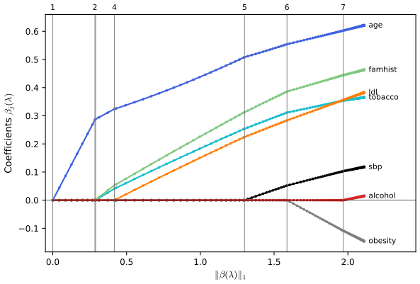
fig_4_13, l1_knots. Reproduces Hastie, Tibshirani and Friedman (2009), Figure 4.13. Download: PDF · SVGBecause the log-likelihood is not quadratic, the profiles are piecewise smooth rather than piecewise linear, so a LAR-type algorithm is harder; the book's figure was made with the predictor–corrector method of glmpath (Park and Hastie, 2007), and coordinate descent on a grid of \(\lambda\) (glmnet) is the usual choice for large problems.
4.4.5 Logistic Regression or LDA?
pp. 127–128 Under the LDA model the log-posterior odds are linear,
\[ \log\frac{\Pr(G=k\given X=x)}{\Pr(G=K\given X=x)}=\log\frac{\pi_k}{\pi_K}-\frac12(\mu_k+\mu_K)^\T\Sigma^{-1}(\mu_k-\mu_K)+x^\T\Sigma^{-1}(\mu_k-\mu_K)=\alpha_{k0}+\alpha_k^\T x, \tag{4.33} \]exactly the form assumed by logistic regression,
\[ \log\frac{\Pr(G=k\given X=x)}{\Pr(G=K\given X=x)}=\beta_{k0}+\beta_k^\T x. \tag{4.34} \]The difference lies in how the coefficients are estimated. The joint density factorises as
\[ \Pr(X,G=k)=\Pr(X)\Pr(G=k\given X), \tag{4.35} \]where, for both models,
\[ \Pr(G=k\given X=x)=\frac{e^{\beta_{k0}+\beta_k^\T x}}{1+\sum_{\ell=1}^{K-1}e^{\beta_{\ell0}+\beta_\ell^\T x}}. \tag{4.36} \]Logistic regression maximises the conditional likelihood and leaves \(\Pr(X)\) arbitrary (effectively estimated by the empirical distribution). LDA maximises the full likelihood of
\[ \Pr(X,G=k)=\phi(X;\mu_k,\Sigma)\pi_k, \tag{4.37} \]in which the marginal
\[ \Pr(X)=\sum_{k=1}^K\pi_k\phi(X;\mu_k,\Sigma) \tag{4.38} \]also depends on the parameters.
Result 4.12 (LDA as a plug-in logistic model, and what the marginal buys) pp. 127–128
(a) The LDA estimates of the logistic coefficients are \(\hat\alpha_k=\hat\Sigma^{-1}(\hat\mu_k-\hat\mu_K)\) and \(\hat\alpha_{k0}\) from (4.33) with the plug-in estimates: maximum likelihood estimates of \(\alpha\) under the joint model, by invariance. (b) The LDA estimates are always finite (when \(\hat\Sigma\) is nonsingular), even when the classes are separable and the logistic maximum likelihood estimate does not exist. (c) If the Gaussian model holds, LDA is asymptotically more efficient; the loss of logistic regression grows with the separation of the classes.
Proof and numbers
(a) The map from \((\pi,\mu,\Sigma)\) to \((\alpha_{k0},\alpha_k)\) is (4.33); the maximum likelihood estimate of a function of the parameters is that function of their maximum likelihood estimates. (b) \(\hat\mu_k\), \(\hat\pi_k\) are averages and \(\hat\Sigma^{-1}\) exists, so \(\hat\alpha\) is a finite closed-form expression; separation plays no role. (c) The full likelihood uses the information in the \(x_i\) about \((\mu,\Sigma)\) as well, including points far from the boundary, which logistic regression nearly ignores (their weights \(p_i(1-p_i)\) are tiny). Efron (1975) computed the asymptotic relative efficiency of logistic regression for the error rate; the book summarises it as a loss of about 30%. A small simulation (two classes \(\N(\pm\frac\Delta2e_1,\bI_2)\), 100 points per class, 1000 replicates, exact error rates; lda_vs_logistic_sim) shows how this depends on \(\Delta\): the ratio of the mean excess errors (LDA over logistic) is 0.99 at \(\Delta=1\), 0.85 at \(\Delta=2\), 0.56 at \(\Delta=3\) and 0.39 at \(\Delta=3.5\). The price is robustness: points far away, including gross outliers, influence \(\hat\Sigma\). Unlabelled observations also carry information about the parameters through (4.38). ∎
In practice the Gaussian assumptions are never exactly right and some inputs are qualitative; logistic regression is often regarded as the safer choice, but the two usually give similar results.
4.5 Separating Hyperplanes
pp. 129–130 Separating hyperplane classifiers construct a linear boundary that tries to separate the classes explicitly; they are the basis of the support vector classifier (Chapter 12 of the book). Figure 4.14 shows 20 separable points with the least squares line (which, for two classes, has the LDA direction) and two perceptron solutions. The least squares boundary is
\[ \{x:\hat\beta_0+\hat\beta_1x_1+\hat\beta_2x_2=0\}. \tag{4.39} \]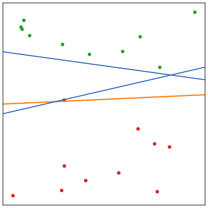
fig_4_14. Reproduces Hastie, Tibshirani and Friedman (2009), Figure 4.14. Download: PDF · SVGResult 4.13 (the linear algebra of a hyperplane; replaces Figure 4.15) p. 130, (4.40)
Let \(L=\{x:f(x)=\beta_0+\beta^\T x=0\}\) with \(\beta\ne0\). (1) For \(x_1,x_2\in L\), \(\beta^\T(x_1-x_2)=0\), so \(\beta^*=\beta/\|\beta\|\) is the unit normal of \(L\). (2) For \(x_0\in L\), \(\beta^\T x_0=-\beta_0\). (3) The signed distance of \(x\) to \(L\) is
\[ \beta^{*\T}(x-x_0)=\frac{1}{\|\beta\|}(\beta^\T x+\beta_0)=\frac{1}{\|f'(x)\|}f(x), \tag{4.40} \]so \(f(x)\) is proportional to the signed distance.
Proof
(1) and (2) are \(f(x_1)-f(x_2)=0\) and \(f(x_0)=0\). (3) Decompose \(x-x_0=s\beta^*+u\) with \(u\perp\beta\); then \(x-s\beta^*=x_0+u\in L\) by (1), and \[\|x-y\|^2=\|s\beta^*+(x_0+u-y)\|^2\ge s^2\] for every \(y\in L\) (the difference \(x_0+u-y\) is orthogonal to \(\beta^*\)), with equality at \(y=x_0+u\). So the distance is \(|s|\) and the sign tells the side, \[s=\beta^{*\T}(x-x_0)=(\beta^\T x-\beta^\T x_0)/\|\beta\|=(\beta^\T x+\beta_0)/\|\beta\|\] by (2); \(f'(x)=\beta\). ∎
4.5.1 Rosenblatt's Perceptron Learning Algorithm
pp. 130–132 With \(y_i\in\{-1,1\}\), a point is misclassified when \(y_i(x_i^\T\beta+\beta_0)\lt0\). The perceptron minimises
\[ D(\beta,\beta_0)=-\sum_{i\in\mathcal M}y_i(x_i^\T\beta+\beta_0), \tag{4.41} \]where \(\mathcal M\) indexes the misclassified points. For fixed \(\mathcal M\),
\[ \frac{\partial D(\beta,\beta_0)}{\partial\beta}=-\sum_{i\in\mathcal M}y_ix_i, \tag{4.42} \] \[ \frac{\partial D(\beta,\beta_0)}{\partial\beta_0}=-\sum_{i\in\mathcal M}y_i, \tag{4.43} \]and stochastic gradient descent visits the misclassified points one at a time:
\[ \begin{pmatrix}\beta\\\beta_0\end{pmatrix}\leftarrow\begin{pmatrix}\beta\\\beta_0\end{pmatrix}+\rho\begin{pmatrix}y_ix_i\\y_i\end{pmatrix}. \tag{4.44} \]Result 4.14 (the perceptron criterion and its convergence; Exercise 4.6) pp. 130–131
(a) \(D\ge0\), and \(D\) is \(\|\beta\|\) times the sum of the distances of the misclassified points to the boundary. (b) If the classes are linearly separable, the updates (4.44) on normalised augmented inputs stop after at most \(\|\beta_{\rm start}-\beta_{\rm sep}\|^2\) steps, at a separating hyperplane. (c) The learning rate \(\rho\) can be taken as 1 when \(\beta_{\rm start}=0\): with any \(\rho>0\) all iterates are scaled by \(\rho\), and the classifications made along the way are the same.
Proof
(a) For \(i\in\mathcal M\), \[-y_i(x_i^\T\beta+\beta_0)=|x_i^\T\beta+\beta_0|=\|\beta\|\cdot\mathrm{dist}(x_i,L)\] by (4.40). (b) is Exercise 4.6. (c) By induction, if every iterate with rate \(\rho\) is \(\rho\) times the iterate with rate 1, the signs \(y_i(x_i^\T\beta+\beta_0)\) are the same, so the same point is updated, and adding \(\rho y_i(x_i,1)\) preserves the relation. With a nonzero start the statement holds with \(\beta_{\rm start}\) also scaled by \(\rho\). ∎
See also (companion course): the perceptron convergence theorem (Result 4.7) of the Bayesian ML course.
The book lists the drawbacks (after Ripley, 1996): with separable data the solution depends on the start (Figure 4.14); the number of steps can be very large when the gap is small (the bound grows like \(1/\text{margin}^2\)); and with non-separable data the algorithm does not converge and cycles, possibly with long cycles. Separation can be forced by enlarging the feature space, but at the risk of over-fitting.
4.5.2 Optimal Separating Hyperplanes
pp. 132–135 The optimal separating hyperplane (Vapnik, 1996) maximises the distance to the closest point:
\[ \max_{\beta,\beta_0,\|\beta\|=1}M\ \ \text{subject to}\ \ y_i(x_i^\T\beta+\beta_0)\ge M,\ i=1,\dots,N. \tag{4.45} \]Dropping the norm constraint, the conditions become
\[ \frac{1}{\|\beta\|}y_i(x_i^\T\beta+\beta_0)\ge M, \tag{4.46} \] \[ y_i(x_i^\T\beta+\beta_0)\ge M\|\beta\|, \tag{4.47} \]and setting \(\|\beta\|=1/M\) gives
\[ \min_{\beta,\beta_0}\frac12\|\beta\|^2\ \ \text{subject to}\ \ y_i(x_i^\T\beta+\beta_0)\ge1,\ i=1,\dots,N. \tag{4.48} \]Result 4.15 ((4.45) and (4.48) are the same problem) p. 132
If the data are separable, (4.48) has a unique solution \((\hat\beta,\hat\beta_0)\), and \((\hat\beta/\|\hat\beta\|,\hat\beta_0/\|\hat\beta\|)\) solves (4.45) with \(M=1/\|\hat\beta\|\). The margin \(M\) is the distance from the boundary to the nearest training point on either side, so the empty slab around the boundary has total width \(2M=2/\|\hat\beta\|\).
Proof
Feasible points of (4.45) with \(M>0\) correspond to feasible points of (4.48) by \((\beta,\beta_0)\mapsto(\beta,\beta_0)/M\) (dividing the constraint by \(M\)), with \(\|\beta/M\|=1/M\); conversely a feasible \((\beta,\beta_0)\) of (4.48) gives \((\beta,\beta_0)/\|\beta\|\) feasible for (4.45) with \(M=1/\|\beta\|\). Maximising \(M\) is therefore minimising \(\|\beta\|\) over (4.48). (4.48) minimises a strictly convex function of \(\beta\) over a nonempty closed convex set, so \(\hat\beta\) is unique; \(\hat\beta_0\) is unique because some constraint is active on each side (otherwise shifting \(\beta_0\) or shrinking \(\beta\) would improve). By (4.40) the constraints say every point has distance at least \(1/\|\beta\|\) from \(L\) on its own side, with equality for the active points of both classes; the slab between the two parallel hyperplanes \(f(x)=\pm1\) therefore has width \(2/\|\beta\|\). (The book calls \(1/\|\beta\|\) the "thickness" of the slab; it is the half-width.) Numerically, a scan of 20000 directions in the plane gives the same maximal margin, 0.1397, as the quadratic programme for the data of Figure 4.16. ∎
The Lagrange (primal) function, minimised over \(\beta,\beta_0\), is
\[ L_P=\frac12\|\beta\|^2-\sum_{i=1}^N\alpha_i[y_i(x_i^\T\beta+\beta_0)-1]. \tag{4.49} \]Setting derivatives to zero,
\[ \beta=\sum_{i=1}^N\alpha_iy_ix_i, \tag{4.50} \] \[ 0=\sum_{i=1}^N\alpha_iy_i, \tag{4.51} \]and substituting gives the Wolfe dual
\[ L_D=\sum_{i=1}^N\alpha_i-\frac12\sum_{i=1}^N\sum_{k=1}^N\alpha_i\alpha_ky_iy_kx_i^\T x_k\ \ \text{subject to}\ \ \alpha_i\ge0\ \text{and}\ \sum_{i=1}^N\alpha_iy_i=0. \tag{4.52} \]The solution also satisfies complementary slackness:
\[ \alpha_i[y_i(x_i^\T\beta+\beta_0)-1]=0\ \ \forall i. \tag{4.53} \]Result 4.16 (the dual of the optimal separating hyperplane, and support points) pp. 133–134, (4.49)–(4.54)
(a) \((\hat\beta,\hat\beta_0)\) solves (4.48) iff there are \(\alpha_i\ge0\) with (4.50), (4.51), (4.53) and primal feasibility (the KKT conditions); \(\alpha\) then maximises (4.52) and the optimal values agree: \(L_D(\hat\alpha)=\frac12\|\hat\beta\|^2\). (b) If \(\alpha_i>0\), \(x_i\) lies on the edge of the slab; points strictly outside it have \(\alpha_i=0\). So \(\hat\beta\) is a combination of the support points, and \(\hat\beta_0=y_s-x_s^\T\hat\beta\) for any support point \(x_s\). (c) The dual depends on the data only through inner products \(x_i^\T x_k\). New points are classified by
\[ \hat G(x)=\sgn\hat f(x),\qquad\hat f(x)=x^\T\hat\beta+\hat\beta_0. \tag{4.54} \]Proof
(a) (4.48) is a convex quadratic programme with affine constraints, so (with a feasible point, i.e. separable data) the KKT conditions are necessary and sufficient and strong duality holds (affine constraints satisfy the linearity constraint qualification; see the convex duality section of the toolkit). The dual function is \(g(\alpha)=\min_{\beta,\beta_0}L_P\). \(L_P\) is linear in \(\beta_0\) with coefficient \(-\sum_i\alpha_iy_i\), so \(g=-\infty\) unless (4.51) holds; then \(L_P\) is a strictly convex quadratic in \(\beta\), minimised where \(\beta-\sum_i\alpha_iy_ix_i=0\), i.e. (4.50). Substituting, \[\frac12\|\beta\|^2-\beta^\T\sum_i\alpha_iy_ix_i+\sum_i\alpha_i=\sum_i\alpha_i-\frac12\|\sum_i\alpha_iy_ix_i\|^2,\] which is (4.52) after expanding the norm. Maximising \(g\) over \(\alpha\ge0\) is the dual; strong duality makes its value \(\frac12\|\hat\beta\|^2\), and complementary slackness (4.53) is the condition for the duality gap to be zero term by term. (b) If \(\alpha_i>0\), (4.53) forces \(y_i(x_i^\T\hat\beta+\hat\beta_0)=1\): distance exactly \(1/\|\hat\beta\|\), the edge of the slab. Then \(y_s(x_s^\T\hat\beta+\hat\beta_0)=1\) and \(y_s^2=1\) give \(\hat\beta_0=y_s-x_s^\T\hat\beta\). (c) is visible in (4.52), and (4.54) uses \(x^\T\hat\beta=\sum_i\hat\alpha_iy_ix^\T x_i\). For Figure 4.16 the dual solved numerically has three support points, the primal and dual values agree to \(10^{-6}\), and the solution coincides with a hard-margin support vector machine. ∎
See also (companion course): Result 7.2 (the dual problem) and Result 7.3 (KKT conditions and support vectors) of the Bayesian ML course, with its SVM demo.
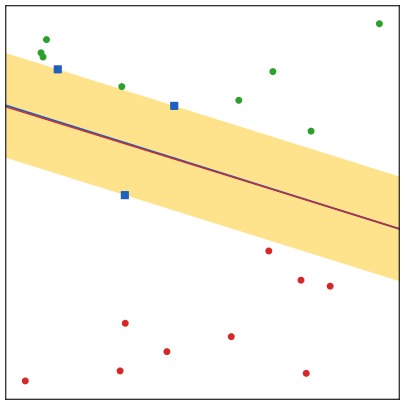
fig_4_16. Reproduces Hastie, Tibshirani and Friedman (2009), Figure 4.16. Download: PDF · SVGFilling the gap 4.11: what "the logistic regression solution" means for separable data p. 134
For separable data the logistic log-likelihood has no maximiser (Exercise 4.5): the line drawn is wherever the iterations were stopped. What can be said: along any separating direction the log-likelihood increases to its supremum 0, and with a ridge penalty \(\frac\lambda2\|\beta\|^2\) the penalised maximiser exists and its direction converges to the optimal separating hyperplane's as \(\lambda\to0\) (Rosset, Zhu and Hastie, 2004), the connection the book develops in Section 12.3.3.
Why, and how fast
If \(y_i(x_i^\T\beta+\beta_0)>0\) for all \(i\), then along \(c(\beta,\beta_0)\), \(c\to\infty\), every term of (4.20) (written for \(\pm1\) labels as \(-\log(1+e^{-y_i c f(x_i)})\)) increases to 0. For large \(c\) the log-likelihood is dominated by the points with the smallest \(y_if(x_i)/\|\beta\|\), i.e. by the margin, which is why the limit direction is the maximum-margin one. The convergence is slow: on the data of Figure 4.16 the angle between the ridge-penalised direction and the optimal one is 19.6, 6.4, 3.7 and 2.9 degrees for \(\lambda=10^{-1},10^{-3},10^{-5},10^{-7}\). ∎
The optimal hyperplane depends only on the support points, which suggests robustness to misspecification far from the boundary; but finding them uses all the data, and if the classes really are Gaussian LDA is optimal and the hyperplane pays for relying on the (noisier) boundary points. Logistic regression shares features with it: its coefficients come from a weighted least squares fit in which points near the boundary get the largest weights. For non-separable data there is no feasible point; the support vector classifier of Chapter 12 allows overlap.
Exercises
All nine exercises of Chapter 4 (Hastie, Tibshirani and Friedman, 2009, pp. 135–137), restated in my own words, with complete solutions (hidden). Numerical statements were confirmed with the chapter's code.
Exercise 4.1. Show how to solve the generalised eigenvalue problem \(\max_a a^\T\bB a\) subject to \(a^\T\bW a=1\) by reducing it to a standard eigenvalue problem.
Solution
Let \(\bW\) be positive definite with symmetric square root \(\bW^{1/2}=\bU\bD^{1/2}\bU^\T\) (from \(\bW=\bU\bD\bU^\T\)); a Cholesky factor \(\bW=\mathbf{R}^\T\mathbf{R}\) works equally well. Put \(b=\bW^{1/2}a\). The constraint becomes \(b^\T b=1\) and the objective \(b^\T\bB^*b\) with \(\bB^*=\bW^{-1/2}\bB\bW^{-1/2}\), symmetric positive semidefinite. Diagonalise \(\bB^*=\bV^*\bD_B\bV^{*\T}\), eigenvalues \(\lambda_1\ge\lambda_2\ge\dots\). For a unit \(b=\sum_jc_jv_j^*\), \(b^\T\bB^*b=\sum_j\lambda_jc_j^2\le\lambda_1\), with equality at \(b=v_1^*\). Hence the maximum is \(\lambda_1\), attained at \(a_1=\bW^{-1/2}v_1^*\). The Lagrange condition \(\bB a=\lambda\bW a\) is equivalent to \(\bB^*b=\lambda b\), so the stationary points are the \(\bW^{-1/2}v_j^*\), and the \(j\)th maximises the objective subject to \(a^\T\bW a=1\) and \(a^\T\bW a_i=0\) for \(i\lt j\) (Result 4.6). This is exactly the book's three-step recipe, so \(a_\ell=v_\ell\). With the Cholesky factor one uses \(\mathbf{R}^{-\T}\bB\mathbf{R}^{-1}\) instead; the eigenvalues are the same and \(a=\mathbf{R}^{-1}b\).
Exercise 4.2. Two classes with sizes \(N_1,N_2\) (\(N=N_1+N_2\)), inputs \(x\in\R^p\), and the response coded \(-N/N_1\) in class 1 and \(N/N_2\) in class 2. (a) Show that LDA classifies to class 2 iff \[x^\T\hat\Sigma^{-1}(\hat\mu_2-\hat\mu_1)>\frac12\hat\mu_2^\T\hat\Sigma^{-1}\hat\mu_2-\frac12\hat\mu_1^\T\hat\Sigma^{-1}\hat\mu_1+\log(N_1/N)-\log(N_2/N).\] (b) Show that the least squares coefficients of \(\sum_i(y_i-\beta_0-\beta^\T x_i)^2\) (4.55) satisfy
\[ \Big[(N-2)\hat\Sigma+\frac{N_1N_2}{N}\hat\Sigma_B\Big]\beta=N(\hat\mu_2-\hat\mu_1),\qquad\hat\Sigma_B=(\hat\mu_2-\hat\mu_1)(\hat\mu_2-\hat\mu_1)^\T. \tag{4.56} \](c) Deduce \(\hat\beta\propto\hat\Sigma^{-1}(\hat\mu_2-\hat\mu_1)\) (4.57). (d) Show this holds for any two distinct codes. (e) Find \(\hat\beta_0\) and show that "class 2 if the fit is positive" is the LDA rule only when \(N_1=N_2\).
Solution
(a) By (4.10) with \(\hat\pi_k=N_k/N\), \(\delta_2(x)>\delta_1(x)\) iff \[x^\T\hat\Sigma^{-1}(\hat\mu_2-\hat\mu_1)-\frac12\hat\mu_2^\T\hat\Sigma^{-1}\hat\mu_2+\frac12\hat\mu_1^\T\hat\Sigma^{-1}\hat\mu_1+\log\frac{N_2}{N}-\log\frac{N_1}{N}>0,\] which rearranges to the stated inequality (4.11).
(b) Eliminating the intercept, \(\hat\beta\) solves \(\mathbf{S}\beta=\sum_i(x_i-\bar x)y_i\) with \(\mathbf{S}=\sum_i(x_i-\bar x)(x_i-\bar x)^\T\). Right side: \[\sum_iy_i=N_1(-N/N_1)+N_2(N/N_2)=0,\] so \[\sum_i(x_i-\bar x)y_i=\sum_iy_ix_i=-\frac{N}{N_1}N_1\hat\mu_1+\frac N{N_2}N_2\hat\mu_2=N(\hat\mu_2-\hat\mu_1).\] Left side: by Filling the gap 4.6, \[\mathbf{S}=\sum_k\sum_{g_i=k}(x_i-\hat\mu_k)(x_i-\hat\mu_k)^\T+\sum_kN_k(\hat\mu_k-\bar x)(\hat\mu_k-\bar x)^\T.\] The first part is \((N-2)\hat\Sigma\). Since \(\bar x=(N_1\hat\mu_1+N_2\hat\mu_2)/N\), \(\hat\mu_1-\bar x=-\frac{N_2}N(\hat\mu_2-\hat\mu_1)\) and \(\hat\mu_2-\bar x=\frac{N_1}N(\hat\mu_2-\hat\mu_1)\), so the second part is \(\big(\frac{N_1N_2^2}{N^2}+\frac{N_2N_1^2}{N^2}\big)\hat\Sigma_B=\frac{N_1N_2}N\hat\Sigma_B\). This is (4.56).
(c) \(\hat\Sigma_B\beta=(\hat\mu_2-\hat\mu_1)\cdot[(\hat\mu_2-\hat\mu_1)^\T\beta]\) is a multiple of \(d=\hat\mu_2-\hat\mu_1\). So \((N-2)\hat\Sigma\beta=\{N-\frac{N_1N_2}N d^\T\beta\}d\) and \(\beta\propto\hat\Sigma^{-1}d\) (4.57). Writing \(\beta=c\hat\Sigma^{-1}d\) and \(\Delta^2=d^\T\hat\Sigma^{-1}d\), (4.56) gives \(c\{(N-2)+\frac{N_1N_2}N\Delta^2\}=N\), so \(c=N/(N-2+N_1N_2\Delta^2/N)>0\).
(d) Any coding \((t_1,t_2)\) with \(t_1\ne t_2\) is an affine function of the one above: \(y'=a+by\) with \(b=(t_2-t_1)/(N/N_1+N/N_2)\ne0\). Least squares is equivariant: the slope vector becomes \(b\hat\beta\), the same direction (reversed if \(b\lt0\)).
(e) \(\hat\beta_0=\bar y-\hat\beta^\T\bar x=-\hat\beta^\T\bar x\), so \(\hat f(x)=\hat\beta^\T(x-\bar x)\) and, as \(c>0\), the rule is \(d^\T\hat\Sigma^{-1}x>d^\T\hat\Sigma^{-1}\bar x\). The LDA threshold in (a) is \(\frac12(\hat\mu_1+\hat\mu_2)^\T\hat\Sigma^{-1}d+\log(N_1/N_2)\). Their difference is \[d^\T\hat\Sigma^{-1}\big[\bar x-\frac{\hat\mu_1+\hat\mu_2}2\big]-\log\frac{N_1}{N_2}=\frac{(N_2-N_1)\Delta^2}{2N}-\log\frac{N_1}{N_2},\] using \(\bar x-\frac{\hat\mu_1+\hat\mu_2}2=\frac{N_2-N_1}{2N}d\). If \(N_1=N_2\) both terms vanish. If \(N_2>N_1\) the first term is positive and \(-\log(N_1/N_2)\) is positive too, so the difference is positive; symmetrically negative if \(N_2\lt N_1\). So the rules coincide iff \(N_1=N_2\) (for \(\Delta>0\)). (Checked numerically with \(N_1=30\), \(N_2=70\), \(p=3\).)
Exercise 4.3. Transform the inputs to \(\hat y=\hat\bB^\T(1,x)\in\R^K\), the fitted values of the indicator regression (4.3). Show that LDA using \(\hat y\) is identical to LDA in the original space.
Solution
Ignore the intercept row of \(\hat\bB\) (a common shift of all \(\hat y\) changes no LDA rule) and write \(\hat y=\mathbf{A}^\T x\), \(\mathbf{A}\) the \(p\times K\) slope part. Let \(\bT\), \(\bW_N\), \(\bB_\pi\) be as in Filling the gap 4.6 and \(m_k=\hat\mu_k-\bar x\). Centring, \(\mathbf{A}=(N\bT)^{-1}\sum_i(x_i-\bar x)y_i^\T\), and \(\sum_i(x_i-\bar x)Y_{ik}=N_km_k\), so the columns of \(\mathbf{A}\) are \(\bT^{-1}\hat\pi_km_k\).
Step 1: LDA after a linear map. For any \(p\times q\) matrix \(\mathbf{A}\), LDA on \(z=\mathbf{A}^\T x\) uses means \(\mathbf{A}^\T\hat\mu_k\) and within covariance \(\mathbf{A}^\T\bW\mathbf{A}\), possibly singular; use its Moore–Penrose inverse. With \(u=\bW^{-1/2}x\), \(\tilde\mu_k=\bW^{-1/2}\hat\mu_k\) and \(\bP\) the orthogonal projection onto \(\mathrm{range}(\bW^{1/2}\mathbf{A})\), one checks \(\bW^{1/2}\mathbf{A}(\mathbf{A}^\T\bW\mathbf{A})^+\mathbf{A}^\T\bW^{1/2}=\bP\), so the discriminant functions become \(u^\T\bP\tilde\mu_k-\frac12\tilde\mu_k^\T\bP\tilde\mu_k+\log\hat\pi_k\). If every \(\tilde\mu_k-\tilde\mu_1\) lies in the range of \(\bP\), then \(\bP(\tilde\mu_k-\tilde\mu_1)=\tilde\mu_k-\tilde\mu_1\), and writing \(\tilde\mu_k=\tilde\mu_1+e_k\) shows that the differences between classes of these functions equal those of the full LDA functions \(u^\T\tilde\mu_k-\frac12\|\tilde\mu_k\|^2+\log\hat\pi_k\) (the terms in \(\tilde\mu_1\) that remain are common to all \(k\)). The condition is: \(\bW^{-1}m_k\in\mathrm{range}(\mathbf{A})\) for all \(k\).
Step 2: the condition holds for indicator regression. \(\mathrm{range}(\mathbf{A})=\bT^{-1}\mathrm{span}\{m_k\}\). We need \(\bT\bW^{-1}m_k\in\mathrm{span}\{m_j\}\) (using \(\bW=\bW_N\); scaling does not matter). Since \(\bT=\bW_N+\bB_\pi\), \[\bT\bW_N^{-1}m_k=m_k+\sum_j\hat\pi_jm_j(m_j^\T\bW_N^{-1}m_k),\] which is in the span. Hence LDA on \(\hat y\) and LDA on \(x\) classify every point identically.
Note that \(\hat y\) always sums to 1 (Filling the gap 4.1), so the within covariance of \(\hat y\) is singular (rank at most \(K-1\)) and an ordinary inverse cannot be used. On the vowel data the within covariance of \(\hat y\) has rank 10 and the two LDA rules agree on all 462 test vectors.
Exercise 4.4. For the \(K\)-class logistic model (4.17), stack all coefficients into a \((p+1)(K-1)\)-vector, define a suitably enlarged input vector, derive the Newton–Raphson algorithm for the multinomial log-likelihood, and describe an implementation.
Solution
Let \(\tilde x_i=(1,x_i^\T)^\T\in\R^{p+1}\), \(\theta=(\beta_1^\T,\dots,\beta_{K-1}^\T)^\T\) with \(\beta_k=(\beta_{k0},\beta_k^\T)^\T\), and define the enlarged \((K-1)\times(p+1)(K-1)\) design block \(\mathbf{X}_i=\bI_{K-1}\otimes\tilde x_i^\T\), so that \(\eta_i=\mathbf{X}_i\theta=(\beta_1^\T\tilde x_i,\dots,\beta_{K-1}^\T\tilde x_i)^\T\). With \(y_i\in\{0,1\}^{K-1}\) the indicators of the first \(K-1\) classes and \(p_i\) the first \(K-1\) probabilities (4.18), the log-likelihood (4.19) is \(\ell(\theta)=\sum_i\{y_i^\T\eta_i-\log(1+\mathbf1^\T e^{\eta_i})\}\). Since \(\partial\log(1+\mathbf1^\T e^\eta)/\partial\eta=p\) and \(\partial p/\partial\eta^\T=\diag(p)-pp^\T\),
\[ \nabla\ell=\sum_i\mathbf{X}_i^\T(y_i-p_i)=\sum_i(y_i-p_i)\otimes\tilde x_i,\qquad \nabla^2\ell=-\sum_i\mathbf{X}_i^\T\mathbf{V}_i\mathbf{X}_i=-\sum_i\mathbf{V}_i\otimes\tilde x_i\tilde x_i^\T, \]with \(\mathbf{V}_i=\diag(p_i)-p_ip_i^\T\), positive definite (a multinomial covariance), so \(\ell\) is concave. The Newton step is \[\theta^{\rm new}=\theta+(\sum_i\mathbf{X}_i^\T\mathbf{V}_i\mathbf{X}_i)^{-1}\sum_i\mathbf{X}_i^\T(y_i-p_i),\] which is again weighted least squares: \(\theta^{\rm new}=(\sum\mathbf{X}_i^\T\mathbf{V}_i\mathbf{X}_i)^{-1}\sum\mathbf{X}_i^\T\mathbf{V}_iz_i\) with \(z_i=\eta_i+\mathbf{V}_i^{-1}(y_i-p_i)\); the weight matrices are not diagonal, which is why the vectorised form is more convenient.
Implementation (
multilogit_newton): start at \(\theta=0\); at each step compute \(\mathbf{E}=\tilde\X\mathbf{B}^\T\) (\(N\times(K-1)\)), the probabilities with a log-sum-exp including the reference column 0, the score \(((\bY-\mathbf{P})^\T\tilde\X)\) flattened, and the Hessian blocks \(\mathbf{H}_{k\ell}=\tilde\X^\T\diag\{p_{ik}(\delta_{k\ell}-p_{i\ell})\}\tilde\X\); solve the linear system (Cholesky), add step halving if the likelihood drops, and stop when the step is negligible. The system has size \((p+1)(K-1)\), 110 for the vowel data, where 11 steps reach the maximum (the same log-likelihood, \(-338.499\), as scikit-learn) and give the logistic row of Table 4.1 (training 0.224, test 0.513). For large \(p\) or \(K\), coordinate descent (glmnet) or quasi-Newton methods avoid forming the Hessian.Exercise 4.5. Two-class logistic regression with \(x\in\R\): describe the maximum likelihood estimates of slope and intercept when the two classes are separated by a point \(x_0\). Generalise to (a) \(x\in\R^p\) and (b) more than two classes.
Solution
Say \(x_i>x_0\) when \(y_i=1\) and \(x_i\lt x_0\) when \(y_i=0\). Every term of (4.20) is \(\log p_i\) or \(\log(1-p_i)\), negative for finite \(\beta\), so \(\ell(\beta)\lt0\). Along \(\beta_1=c\), \(\beta_0=-cx_0\), \(c\to\infty\): \(p_i=\sigma(c(x_i-x_0))\to1\) for \(y_i=1\) and \(\to0\) for \(y_i=0\), so \(\ell\to0=\sup\ell\). The supremum is not attained: the MLE does not exist; any maximising sequence has slope \(\to+\infty\), and the boundary \(-\beta_0/\beta_1\) can converge to any point of the gap between the largest \(x\) of class 0 and the smallest of class 1 (Newton's iterates diverge, and the fitted probabilities tend to 0 and 1).
(a) If a hyperplane separates the classes, \(y_i(\beta^\T x_i+\beta_0)>0\) for some \((\beta,\beta_0)\) (labels \(\pm1\)), and scaling by \(c\to\infty\) drives \(\ell\to0\) as before: no maximiser, \(\|\hat\beta\|\to\infty\) along a separating direction (Figure 4.16; the deviance of the IRLS iterate there is \(6\times10^{-10}\)). If the separation is only quasi-complete (some points on the hyperplane), the same happens for the coefficients of the separated part.
(b) For \(K\) classes, if there are \(\beta_1,\dots,\beta_K\) (with \(\beta_K=0\)) such that each \(x_i\) has \(\beta_{g_i}^\T\tilde x_i>\beta_k^\T\tilde x_i\) for all \(k\ne g_i\) (the classes are separable by a linear multiclass rule), then scaling all \(\beta_k\) by \(c\to\infty\) sends every \(p_{g_i}(x_i)\to1\) and \(\ell\to0\); the multinomial MLE does not exist.
Exercise 4.6. Let \(x_i^*=(x_i,1)\) and \(z_i=x_i^*/\|x_i^*\|\), labels \(y_i\in\{-1,1\}\), and suppose the classes are linearly separable. (a) Show there is \(\beta_{\rm sep}\) with \(y_i\beta_{\rm sep}^\T z_i\ge1\) for all \(i\). (b) For the update \(\beta^{\rm new}=\beta^{\rm old}+y_iz_i\) at a misclassified \(z_i\), show \(\|\beta^{\rm new}-\beta_{\rm sep}\|^2\le\|\beta^{\rm old}-\beta_{\rm sep}\|^2-1\), and conclude that the perceptron stops after at most \(\|\beta_{\rm start}-\beta_{\rm sep}\|^2\) steps.
Solution
(a) Separability means some \(\beta\) has \(y_i\beta^\T x_i^*>0\) for all \(i\); dividing by \(\|x_i^*\|>0\) keeps the sign, so \(m=\min_iy_i\beta^\T z_i>0\) (a finite minimum). Then \(\beta_{\rm sep}=\beta/m\) works. (The book says "in general position"; what is needed is separability.)
(b) Misclassified means \(y_i\beta^{{\rm old}\T}z_i\le0\). Using \(\|z_i\|=1\) and \(y_i^2=1\),
\[ \|\beta^{\rm old}+y_iz_i-\beta_{\rm sep}\|^2=\|\beta^{\rm old}-\beta_{\rm sep}\|^2+2y_i\beta^{{\rm old}\T}z_i-2y_i\beta_{\rm sep}^\T z_i+1\le\|\beta^{\rm old}-\beta_{\rm sep}\|^2+0-2+1. \]Each update reduces the nonnegative quantity \(\|\beta-\beta_{\rm sep}\|^2\) by at least 1, so there can be at most \(\|\beta_{\rm start}-\beta_{\rm sep}\|^2\) updates; after the last one no point is misclassified, i.e. the current \(\beta\) separates the data. Choosing \(\beta_{\rm sep}\) as the optimal hyperplane rescaled gives \(\|\beta_{\rm sep}\|=1/\gamma\) with \(\gamma\) the margin of the normalised points, so from \(\beta_{\rm start}=0\) the bound is \(1/\gamma^2\) (Novikoff's theorem): small gaps mean many steps. On the data of Figure 4.14, from a random start, 12 updates were needed against a bound of 189.
Exercise 4.7. Consider \(D^*(\beta,\beta_0)=-\sum_{i=1}^Ny_i(x_i^\T\beta+\beta_0)\) (4.58), the perceptron criterion summed over all observations, minimised subject to \(\|\beta\|=1\). Describe it in words. Does it solve the optimal separating hyperplane problem?
Solution
By (4.40), with \(\|\beta\|=1\), \(y_i(x_i^\T\beta+\beta_0)\) is the signed distance of \(x_i\) to the hyperplane, positive on the correct side. So \(D^*\) is minus the total signed distance of all points: minimising it pushes the points, on average, as far as possible to their correct sides. Write \(D^*=-\beta^\T\sum_iy_ix_i-\beta_0\sum_iy_i\). If \(N_+\ne N_-\), then \(\sum_iy_i\ne0\) and \(D^*\to-\infty\) as \(\beta_0\to\pm\infty\): there is no minimiser. If \(N_+=N_-=N/2\), \(\beta_0\) drops out (any value) and the minimiser over the unit sphere is \(\beta=s/\|s\|\) with \(s=\sum_iy_ix_i=\frac N2(\bar x_+-\bar x_-)\): the direction joining the class means, which ignores the covariance (Figure 4.9) and depends on all points equally. It is not the optimal separating hyperplane, which depends only on the support points and need not even separate the data. On the data of Figure 4.14 (10 points per class) the mean-difference direction differs from the optimal one by more than 5 degrees.
Exercise 4.8. In the model \(X\given G=k\sim\N(\mu_k,\Sigma)\), add the restriction that the centroids span an affine subspace of dimension \(L\lt\min(K-1,p)\) (the book prints "max", see the corrections). Derive the constrained maximum likelihood estimates of the \(\mu_k\) and \(\Sigma\), and show that the Bayes rule of the fitted model is classification in the reduced LDA subspace (Hastie and Tibshirani, 1996b).
Solution
Profile out \(\Sigma\). With \(\hat\pi_k=N_k/N\) and any centroids \(\mu_k\), the residual scatter is \[\mathbf{S}(\mu)=\frac1N\sum_i(x_i-\mu_{g_i})(x_i-\mu_{g_i})^\T=\bW_N+\sum_k\hat\pi_k(\hat\mu_k-\mu_k)(\hat\mu_k-\mu_k)^\T\] (expand around the class means; the cross terms vanish). As in Filling the gap 4.3, the maximising \(\Sigma\) is \(\mathbf{S}(\mu)\) and the profile log-likelihood is \(-\frac N2\log|\mathbf{S}(\mu)|-\frac{Np}2+\text{const}\). So we must minimise \(\log|\mathbf{S}(\mu)|\) over centroids in an \(L\)-dimensional affine subspace.
Sphere. Put \(y_k=\bW_N^{-1/2}(\hat\mu_k-\bar x)\), \(\nu_k=\bW_N^{-1/2}(\mu_k-\bar x)\), \(e_k=y_k-\nu_k\), and \(\bB^*=\sum_k\hat\pi_ky_ky_k^\T\) (note \(\sum_k\hat\pi_ky_k=0\)), with eigenvalues \(\lambda_1\ge\dots\ge\lambda_p\) and eigenvectors \(v_\ell^*\). Then \(\log|\mathbf{S}|=\log|\bW_N|+\log|\bI+\mathbf{R}|\), \(\mathbf{R}=\sum_k\hat\pi_ke_ke_k^\T\), and the \(\nu_k\) range over an \(L\)-dimensional affine subspace \(c+\mathcal{S}\).
Fixed subspace. Let \(\bP\) project onto \(\mathcal{S}\). Split \(e_k=a_k+b_k\) with \(a_k=(\bI-\bP)(y_k-c)\perp\mathcal{S}\) and \(b_k\in\mathcal{S}\). With \(\mathbf{E}=[e_k\sqrt{\hat\pi_k}]\), \(|\bI_p+\mathbf{E}\mathbf{E}^\T|=|\bI_K+\mathbf{E}^\T\mathbf{E}|\) and \(\mathbf{E}^\T\mathbf{E}=\mathbf{A}^\T\mathbf{A}+\mathbf{B}^\T\mathbf{B}\succeq\mathbf{A}^\T\mathbf{A}\) (the cross terms vanish because \(a_j\perp b_k\)); determinants are monotone in the Loewner order on positive definite matrices, so the best choice has \(b_k=0\), i.e. \(\nu_k\) the orthogonal projection of \(y_k\) onto \(c+\mathcal{S}\). Moreover, because \(\sum_k\hat\pi_ky_k=0\), \[\sum_k\hat\pi_ka_ka_k^\T=(\bI-\bP)(\bB^*+cc^\T)(\bI-\bP)\succeq(\bI-\bP)\bB^*(\bI-\bP),\] so \(c\in\mathcal{S}\) (e.g. \(c=0\), the centroids' weighted mean) is optimal. The minimum over \(\mathcal{S}\) is thus \(\log|\bI+(\bI-\bP)\bB^*(\bI-\bP)|\).
Best subspace. The nonzero eigenvalues of \((\bI-\bP)\bB^*(\bI-\bP)\) are those of the compression of \(\bB^*\) to the \((p-L)\)-dimensional space \(\mathcal{S}^\perp\); by the Poincaré separation (interlacing) theorem the \(j\)th largest of them is at least \(\lambda_{j+L}\). Hence \[\log|\bI+(\bI-\bP)\bB^*(\bI-\bP)|\ge\sum_{\ell>L}\log(1+\lambda_\ell),\] with equality when \(\mathcal{S}=\mathrm{span}(v_1^*,\dots,v_L^*)\). So
\[ \hat\mu_k=\bar x+\bW_N^{1/2}\bV_L^*\bV_L^{*\T}\bW_N^{-1/2}(\hat\mu_k-\bar x),\qquad \hat\Sigma=\bW_N^{1/2}\Big(\bI+\sum_{\ell>L}\lambda_\ell v_\ell^*v_\ell^{*\T}\Big)\bW_N^{1/2}, \]and \[\log|\hat\Sigma|=\log|\bW_N|+\sum_{\ell>L}\log(1+\lambda_\ell).\] (On the vowel data with \(L=2\) a direct numerical minimisation over all centroid configurations reaches the same value, \(-14.12393\).)
Bayes rule. In sphered coordinates \(u=\bW_N^{-1/2}(x-\bar x)\), the fitted model has means \(\bP_Ly_k\) (\(\bP_L=\bV_L^*\bV_L^{*\T}\)) and covariance \(\bI+\sum_{\ell>L}\lambda_\ell v_\ell^*v_\ell^{*\T}\), whose inverse is \(\bP_L+\sum_{\ell>L}(1+\lambda_\ell)^{-1}v_\ell^*v_\ell^{*\T}\). Since \(v_\ell^{*\T}\bP_Ly_k=0\) for \(\ell>L\),
\[ (u-\bP_Ly_k)^\T\hat\Sigma_u^{-1}(u-\bP_Ly_k)=\|\bP_L(u-y_k)\|^2+\sum_{\ell>L}\frac{(v_\ell^{*\T}u)^2}{1+\lambda_\ell}. \]The last sum and \(\log|\hat\Sigma|\) are the same for every class, so the Bayes rule is \(\argmin_k\{\|\bP_L(u-y_k)\|^2-2\log\hat\pi_k\}\): nearest centroid in the first \(L\) discriminant coordinates, which is reduced-rank LDA. (With \(\bW_N\) the distances are scaled by \(N/(N-K)\) relative to the \(\bW\) of Section 4.3.3; with equal priors, as for the vowel data, this changes nothing, and there the Bayes rule of the fitted rank-2 model and reduced-rank LDA with \(L=2\) agree on all test vectors.)
Exercise 4.9. Write a program for quadratic discriminant analysis (one Gaussian per class), apply it to the vowel data and compute the test error.
Solution
The function
qda_scoresof the chapter code computes (4.12) for every class: the class means, the class covariance matrices (divisor \(N_k-1\)), \(\log|\hat\Sigma_k|\) from a determinant (or the eigenvalues, Section 4.3.2), and the quadratic form through \(\hat\Sigma_k^{-1}\), plus \(\log\hat\pi_k\); the class with the largest score wins. On the vowel data (48 training vectors per class in 10 dimensions, so every \(\hat\Sigma_k\) is invertible) the training error is 0.011 and the test error 0.528, the value 0.53 of Table 4.1; the predictions agree with scikit-learn's QDA on every test vector. The near-zero training error and the 52.8% test error show how much the 660 parameters overfit; RDA (Figure 4.7) brings the test error down to 0.45.
Corrections to the book
Found while writing these notes; each is checked by direct algebra or numerically (details in the linked boxes).
- p. 105, on the closest-target rule (4.6): it equals the largest-fit rule (4.4) for any fitted vector; it does not "require that the fitted values sum to 1" (Filling the gap 4.1).
- p. 105: "if there were four rather than three classes lined up like this, a quadratic would not come down fast enough, and a cubic would be needed". For four equally spaced classes of equal size a quadratic already unmasks every class (hat-matrix diagonal 0.55 against at most 0.45 off it); the general rule "degree up to \(K-1\)" is a valid upper bound but far from tight (Filling the gap 4.2).
- p. 114: "\(\bB+\bW=\bT\)" holds only with matching conventions (divisor \(N\) throughout and centroids weighted by \(N_k/N\)), not with \(\bW\) divided by \(N-K\) as defined on p. 109 (Filling the gap 4.6).
- p. 132: the slab defined by the constraints of (4.48) has total width \(2/\|\beta\|\); \(1/\|\beta\|\) is the margin on each side (Result 4.15).
- Exercise 4.6: the hypothesis needed is linear separability, not "general position".
- Exercise 4.8: the restriction should read \(L\lt\min(K-1,p)\) (the centroids always span at most \(\min(K-1,p)\) dimensions, so with "max" the restriction can be vacuous); also "rank" should be the dimension of the affine span of the centroids.
- Tables 4.2 and 4.3: refitting the book's data reproduces every coefficient and standard error, but four Z scores of Table 4.2 differ in the third decimal (intercept \(-4.283\), ldl 3.218, famhist 4.177, age 4.181) and the intercept Z of Table 4.3 is \(-8.44\) (\(=-4.2043/0.4983\)), not \(-8.45\).
Demonstrations for this chapter
Each demonstration runs in the browser, on the book's data or a seeded simulation, and links back to these notes. The ▶ Demo boxes above open them already set to the case under discussion.
| Demonstration | What you can see | Sections and results |
|---|---|---|
| Masking: indicator regression versus LDA | Three to five Gaussian classes on a line or a circle; class regions of indicator regression (polynomial degree 1–4) and of LDA; the fitted indicators along the centroid line; per-class hit rates. Presets: 1 three classes, linear; 2 quadratic; 3 four classes, quadratic; 4 five classes, quadratic; 5 centroids on a circle. | 4.2; Filling the gaps 4.1, 4.2 |
| Reduced-rank LDA on the vowel data | Any pair of discriminant coordinates for training or test data, the classifier with \(L=1,\dots,10\) coordinates (regions when it lives in the plane shown), training and test error against \(L\), and the between-class variance of each coordinate. Presets: 1 Figure 4.4; 2 Figure 4.11; 3 \(L=1\); 4 coordinates 9 and 10; 5 test data. | 4.3.2, 4.3.3; Results 4.5–4.7 |
| Logistic regression: IRLS and the L1 path | IRLS step by step on the heart disease data (deviance, coefficients, the weighted regression of each step), any subset of variables with Z scores and the deviance test; the L1 path with the generalised correlations at any \(\lambda\). Presets: 1 first step; 2 Table 4.2; 3 Table 4.3; 4 two active variables; 5 near the unpenalised fit. | 4.4.1–4.4.4; Results 4.8, 4.9, 4.11 |
Related demonstrations in the companion courses: linear classifiers and logistic regression (Bayesian and Probabilistic Machine Learning); generative classifiers and logistic and softmax regression (Foundations of Deep Learning). The Python code that produces every figure of this page is code/ch04_linear_classification.py (see the code index).
References
- Hastie, T., Tibshirani, R. and Friedman, J. (2009). The Elements of Statistical Learning: Data Mining, Inference, and Prediction, 2nd edition. Springer, New York. Chapter 4, pp. 101–137. hastie.su.domains/ElemStatLearn.
- Boyd, S. and Vandenberghe, L. (2004). Convex Optimization. Cambridge University Press.
- Efron, B. (1975). The efficiency of logistic regression compared to normal discriminant analysis. Journal of the American Statistical Association, 70, 892–898.
- Fisher, R. A. (1936). The use of multiple measurements in taxonomic problems. Annals of Eugenics, 7, 179–188.
- Friedman, J. (1989). Regularized discriminant analysis. Journal of the American Statistical Association, 84, 165–175.
- Friedman, J., Hastie, T. and Tibshirani, R. (2010). Regularization paths for generalized linear models via coordinate descent. Journal of Statistical Software, 33(1), 1–22.
- Hastie, T. and Tibshirani, R. (1996b). Discriminant analysis by Gaussian mixtures. Journal of the Royal Statistical Society, Series B, 58, 155–176.
- McCullagh, P. and Nelder, J. A. (1989). Generalized Linear Models, 2nd edition. Chapman and Hall, London.
- Michie, D., Spiegelhalter, D. and Taylor, C. (eds) (1994). Machine Learning, Neural and Statistical Classification. Ellis Horwood.
- Novikoff, A. B. J. (1962). On convergence proofs on perceptrons. Proceedings of the Symposium on the Mathematical Theory of Automata, 12, 615–622.
- Park, M. Y. and Hastie, T. (2007). L1-regularization path algorithm for generalized linear models. Journal of the Royal Statistical Society, Series B, 69, 659–677.
- Ripley, B. D. (1996). Pattern Recognition and Neural Networks. Cambridge University Press.
- Rosenblatt, F. (1958). The perceptron: a probabilistic model for information storage and organization in the brain. Psychological Review, 65, 386–408.
- Rosset, S., Zhu, J. and Hastie, T. (2004). Margin maximizing loss functions. Advances in Neural Information Processing Systems, 16.
- Rousseauw, J., du Plessis, J., Benade, A., Jordaan, P., Kotze, J. and Ferreira, J. (1983). Coronary risk factor screening in three rural communities. South African Medical Journal, 64, 430–436.
- Vapnik, V. (1996). The Nature of Statistical Learning Theory. Springer, New York.
The numerical statements in the text (Tables 4.1–4.3, the masking analysis, the discriminant coordinates and their optimality, the constrained maximum likelihood of Exercise 4.8, the IRLS and score-test identities, the L1 optimality conditions and knots, and the optimal separating hyperplane and its dual) were confirmed numerically.