Expectation
The expectation of a random variable compresses its whole distribution into one number, the long-run average of independent draws. This chapter builds the arithmetic of that number: when it exists, how to compute the expectation of a function of a random variable without finding the function's distribution, why expectations of sums are sums of expectations while products need independence, and how the variance and covariance measure spread and linear association. It then computes the means and variances of the standard distributions, extends everything to random vectors (the mean vector and covariance matrix, and how they change under linear maps), treats conditional expectation as a random variable in its own right (iterated expectations and the law of total variance), and closes with the moment generating function, the tool that turns sums of independent variables into products and identifies their distributions.
Ch. 1 Probability Ch. 2 Random variables Ch. 3 Expectation Ch. 4 Inequalities Ch. 5 Convergence Ch. 6 Models and inference Ch. 7 Estimating the CDF Ch. 8 Bootstrap Ch. 9 Parametric inference Ch. 10 Hypothesis testing Ch. 11 Bayesian inference Ch. 12 Decision theory Ch. 13 Regression Ch. 14 Multivariate models Ch. 15 Independence Ch. 16 Causal inference Ch. 17 Directed graphs Ch. 18 Undirected graphs Ch. 19 Log-linear models Ch. 20 Curve estimation Ch. 21 Orthogonal functions Ch. 22 Classification Ch. 23 Stochastic processes Ch. 24 Simulation
How to read these notes
They follow the book. Sections carry the book's numbers (3.1, 3.2, ...), and every displayed equation that the book numbers carries the book's own number, e.g. \((3.15)\). Theorems, lemmas and examples are referred to by the book's numbers (Theorem 3.17, Example 3.28); the results of these notes are numbered separately (Result 3.7) and each says which statement of the book it is.
Filling the gaps. This chapter states most of its results without proof: linearity, the product rule, the properties of the variance and covariance, the unbiasedness of the sample variance, the law of total variance, the properties and the uniqueness of moment generating functions. Every one is proved below, either in the proof attached to its result or in an orange Filling the gap box. Proofs start hidden: open one with its bar, or use the button below.
Figures and demonstrations. The chapter itself has no figures. Its three computer experiments (Exercises 3.9, 3.11 and 3.19) and its main identities are illustrated by six supplementary figures, 3.S1 to 3.S6, made by the Python code. The ▶ Demo boxes open an interactive demonstration already set to the case being discussed.
Main reference
L. Wasserman, All of Statistics: A Concise Course in Statistical Inference, Springer (2004), Chapter 3, pages 47–61 (book website, with the data sets and the author's errata: www.stat.cmu.edu/~larry/all-of-statistics). Section, equation, theorem, example and exercise numbers below refer to this book. Further reading is listed in the references.
The explanations, derivations, figures and code are my own; equations are cited by their numbers in the book.
Companion courses
Expectation is used everywhere on this site, and several companion courses prove parts of this chapter in their own notation. The overlapping material is:
- Sections 3.1–3.3 (expectation, variance, covariance and their identities): Foundations of Deep Learning, Section 2.2.2 and Filling the gap 2.4 (covariance identities, independence and correlation); Bayesian and Probabilistic Machine Learning, Section 1.2.2 and Result 1.3.
- Theorem 3.17 (the sample variance and the divisor \(n-1\)): Result 1.8 of Bayesian and Probabilistic Machine Learning, Result 2.4 and Filling the gap 2.6 of Foundations of Deep Learning, and the first-year notes Why \(n-1\)?
- Section 3.4 (the means and variances of the standard distributions): Results 2.1 (Bernoulli, binomial), 2.2 (beta), 2.5 (multinomial), 2.17 (gamma) and 2.19 (Student's t) of Bayesian and Probabilistic Machine Learning; Results 3.2 (binomial) and 3.3 (multinomial) of Foundations of Deep Learning.
- The multivariate normal's mean and covariance: Result 3.5 of Foundations of Deep Learning and Result 2.7 of Bayesian and Probabilistic Machine Learning.
- Section 3.5 (conditional expectation and variance): Result 2.4 and Result 2.21 (moments of a mixture) of Bayesian and Probabilistic Machine Learning, Exercise 2.11 of Foundations of Deep Learning, and the overdispersed counts of Statistical Methods for Modern Biology (the beta-binomial, mixture moments).
- Section 3.6 (moment generating functions): the first-year notes Moment generating functions and the normal family, which use the uniqueness theorem without proof.
Where a proof there is the same, these notes give the statement and a short argument and link to it. New here: a correct argument that the Cauchy distribution has no mean (Filling the gap 3.1), the variance of \(S_n^2\) for non-normal data and the divisor that minimises its mean squared error (Filling the gap 3.2), linear maps of the multivariate normal (Filling the gap 3.7), the justification for differentiating a moment generating function under the expectation (Filling the gap 3.10), why the moment generating function determines the distribution (Filling the gap 3.12), and two slips in the text (notes on the text).
The chapter at a glance
- 3.1 \(\E(X)=\int x\,\d F(x)\) exists when \(\E|X|<\infty\) (Definition 3.1); the Cauchy distribution has no mean (Filling the gap 3.1); \(\E\,r(X)=\int r(x)\,\d F(x)\) without finding the law of \(r(X)\) (Result 3.1); a finite \(k\)th moment gives finite lower moments (Result 3.2).
- 3.2 Expectation is linear, always (Result 3.3); it is multiplicative for independent variables (Result 3.4).
- 3.3 The rules for the variance (Result 3.5); \(\V(X)=0\) only for constants (Result 3.6); \(\E(S_n^2)=\sigma^2\) (Result 3.7), although \(n-1\) is rarely the divisor with the smallest error (Filling the gap 3.2); \(|\rho|\le1\) with equality only for exact linear relations (Result 3.8); the variance of a sum (Result 3.9).
- 3.4 The table of means and variances, derived (Filling the gaps 3.4, 3.5); \(\E(\bA\bX)=\bA\bmu\) and \(\V(\bA\bX)=\bA\bSigma\bA^\T\) (Result 3.10); the multinomial covariances (Filling the gap 3.6); linear maps of the multivariate normal (Filling the gap 3.7).
- 3.5 \(\E(Y\given X)\) is a random variable (Definition 3.7, Filling the gap 3.8); \(\E\,\E(Y\given X)=\E(Y)\) (Result 3.11); \(\V(Y)\)\({}=\E\,\V(Y\given X)+\V\,\E(Y\given X)\) (Result 3.12).
- 3.6 \(\psi^{(k)}(0)=\E(X^k)\) (Filling the gap 3.10); mgfs of independent sums multiply (Result 3.13); an mgf determines the distribution (Result 3.14, Filling the gap 3.12).
Notation. \(F\) or \(F_X\) is a cumulative distribution function and \(f\) or \(f_X\) a probability mass or density function. \(\E\) is expectation, \(\V\) variance, \(\Cov\) covariance, \(\P\) probability; \(I_A\) is the indicator of the set \(A\). Random vectors are bold: \(\bX=(X_1,\dots,X_k)^\T\). \(X\deq Y\) means that \(X\) and \(Y\) have the same distribution. Gamma and exponential distributions use the book's scale parameter \(\beta\): \(\mathrm{Gamma}(\alpha,\beta)\) has density \(x^{\alpha-1}e^{-x/\beta}/\{\Gamma(\alpha)\beta^\alpha\}\) and mean \(\alpha\beta\).
Prerequisites. Random variables, distribution functions, densities, joint and conditional distributions and independence (Chapter 2 of the book; notes for Chapter 2).
3.1 Expectation of a Random Variable
pp. 47–50 The mean of a random variable is a weighted average of its possible values, the weights being their probabilities.
See also (companion courses): Section 2.2.2 of Foundations of Deep Learning and Section 1.2.2 of Bayesian and Probabilistic Machine Learning; the first-year notes Expectation and variance.
Definition 3.1 (expectation; Definition 3.1 of the book) pp. 47–48, (3.1)–(3.2)
The expected value, mean or first moment of \(X\) is
\[ \E(X)=\int x\,\d F(x)=\begin{cases}\sum_x x f(x)&\text{if }X\text{ is discrete,}\\[2pt] \int x f(x)\,\d x&\text{if }X\text{ is continuous,}\end{cases} \tag{3.1} \] \[ \E(X)=\E X=\int x\,\d F(x)=\mu=\mu_X. \tag{3.2} \]We say that \(\E(X)\) exists if \(\int|x|\,\d F_X(x)<\infty\); otherwise the expectation does not exist.
The notation \(\int x\,\d F(x)\) covers sums and integrals at once (and mixtures of the two); Section 3.7 says what it means in general. The requirement \(\E|X|<\infty\) is not pedantry. A sum \(\sum_x xf(x)\) over infinitely many values, or an integral over an unbounded range, has a value that does not depend on how it is computed only when it converges absolutely; with \(\E|X|<\infty\) both the positive part \(\int_{x>0}x\,\d F\) and the negative part \(\int_{x<0}|x|\,\d F\) are finite and \(\E(X)\) is their difference.
Examples 3.2–3.4 compute three means directly: \(\E(X)=p\) for \(X\sim\mathrm{Bernoulli}(p)\); \(\E(X)\)\({}=0\cdot\tfrac14+1\cdot\tfrac12+2\cdot\tfrac14\)\({}=1\) for the number of heads in two fair tosses; and \(\E(X)\)\({}=\tfrac14\int_{-1}^3x\,\d x\)\({}=1\) for \(X\sim\Unif(-1,3)\), the midpoint of the interval. Example 3.5 shows that a mean need not exist.
Filling the gap 3.1: the Cauchy distribution has no mean, and why the running average never settles p. 48, Example 3.5
For the Cauchy density \(f(x)=1/\{\pi(1+x^2)\}\), \(\int|x|\,\d F(x)=\infty\). The positive and negative parts of the mean are both infinite, so \(\E(X)\) is not defined at all (not even as \(+\infty\)).
Proof
By symmetry, \(\int|x|f(x)\,\d x\)\({}=\frac2\pi\int_0^\infty\frac{x}{1+x^2}\,\d x\). For \(M>0\), the substitution \(u=1+x^2\) gives
\[ \int_0^M\frac{x}{1+x^2}\,\d x=\frac12\log(1+M^2)\xrightarrow[M\to\infty]{}\infty. \]The integrand is non-negative, so the integral over \([0,\infty)\) is the increasing limit of these truncated integrals and is infinite. The same computation on \((-\infty,0]\) shows that \(\int_{x>0}x\,\d F\)\({}=\int_{x<0}|x|\,\d F\)\({}=\infty\): the "mean" would be \(\infty-\infty\), which has no value. A symmetric truncation \(\int_{-M}^Mxf(x)\,\d x=0\) for every \(M\) does not rescue it, because an asymmetric one, \(\int_{-M}^{2M}xf(x)\,\d x\)\({}=\tfrac1{2\pi}\log\frac{1+4M^2}{1+M^2}\to\tfrac{\log4}{2\pi}\), has a different limit: the answer depends on how the integral is cut off, which is exactly what absolute convergence rules out.
A remark on the book's argument. The book integrates by parts and obtains \([x\tan^{-1}x]_0^\infty-\int_0^\infty\tan^{-1}x\,\d x\). Both terms are infinite, so this expression is \(\infty-\infty\) and by itself proves nothing; the computation above, which never subtracts infinities, is the clean version. (It also needs no integration by parts.)
Why the running average wanders. If \(X_1,\dots,X_n\) are independent standard Cauchy variables, their average \(\overline X_n\) is again standard Cauchy for every \(n\) (its characteristic function is \(e^{-|t|}\), the same as that of one \(X_i\)). The average therefore never concentrates: a single huge draw, which happens with probability \(\P(|X|>x)\approx2/(\pi x)\), moves it far away, as in Figure 3.S1(b). The law of large numbers (Chapter 5) needs \(\E|X|<\infty\), and the Cauchy shows that this assumption cannot simply be dropped. ∎
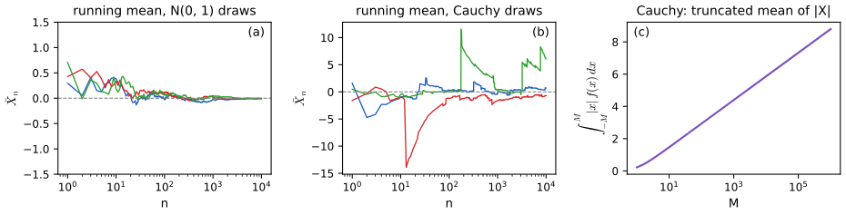
fig_3_s1. Supplementary figure for Wasserman (2004), Example 3.5 and Exercise 3.9. Download: PDF · SVGFrom now on, as in the book, every expectation that is written down is assumed to exist. To compute the mean of \(Y=r(X)\) one could first find the distribution of \(Y\). The next result says that this is never necessary.
Result 3.1 (the rule of the lazy statistician; Theorem 3.6) p. 48, (3.3)–(3.4)
Let \(Y=r(X)\). Then
\[ \E(Y)=\E\big(r(X)\big)=\int r(x)\,\d F_X(x), \tag{3.3} \]in the sense that \(\E(Y)\) exists if and only if \(\int|r(x)|\,\d F_X(x)<\infty\), and then the two sides agree. In particular \(\E\,I_A(X)=\P(X\in A)\): probability is a special case of expectation. For a function of two variables, \(Z=r(X,Y)\),
\[ \E(Z)=\E\big(r(X,Y)\big)=\iint r(x,y)\,\d F(x,y). \tag{3.4} \]Proof (the book gives none; Exercise 3.6 asks for the discrete case)
Discrete \(X\). Let \(X\) take the values \(x_1,x_2,\dots\) and let \(Y=r(X)\) take the distinct values \(y_1,y_2,\dots\). The events \(\{Y=y_j\}\) are the disjoint unions \(\{Y\)\({}=y_j\}\)\({}=\bigcup_{i:\,r(x_i)=y_j}\{X\)\({}=x_i\}\), so \(f_Y(y_j)\)\({}=\sum_{i:\,r(x_i)=y_j}f_X(x_i)\). Grouping the terms of a series of non-negative terms does not change its sum, so
\[ \sum_i|r(x_i)|f_X(x_i)=\sum_j\sum_{i:\,r(x_i)=y_j}|y_j|f_X(x_i)=\sum_j|y_j|f_Y(y_j)=\E|Y|. \]Hence \(\E|Y|<\infty\) exactly when \(\sum_i|r(x_i)|f_X(x_i)<\infty\). In that case the series \(\sum_ir(x_i)f_X(x_i)\) converges absolutely, an absolutely convergent series may be regrouped freely, and the same grouping gives \(\sum_ir(x_i)f_X(x_i)\)\({}=\sum_jy_jf_Y(y_j)\)\({}=\E(Y)\).
General \(X\) (for example continuous). First let \(r\ge0\), so \(Y\ge0\). For any non-negative random variable, \(\E(Y)\)\({}=\int_0^\infty\P(Y>t)\,\d t\) (the tail formula of Exercise 3.7, proved there for every non-negative variable by exchanging two integrals of a non-negative function, which Tonelli's theorem allows). Applying it and exchanging the order of integration once more,
\[ \begin{aligned}\E(Y)&=\int_0^\infty\P\big(r(X)>t\big)\,\d t\\&=\int_0^\infty\!\!\int I\{r(x)>t\}\,\d F_X(x)\,\d t\\&=\int\!\!\int_0^{\infty}I\{t<r(x)\}\,\d t\,\d F_X(x)\\&=\int r(x)\,\d F_X(x).\end{aligned} \]Both sides may be \(+\infty\); the identity holds anyway. For a general \(r\) write \(r=r^+-r^-\) with \(r^+=\max(r,0)\) and \(r^-=\max(-r,0)\). Then \(Y^+=r^+(X)\) and \(Y^-=r^-(X)\), the non-negative case gives \(\E Y^\pm=\int r^\pm\,\d F_X\), and \(\E|Y|\)\({}=\E Y^++\E Y^-\)\({}=\int|r|\,\d F_X\). When this is finite, \(\E(Y)\)\({}=\E Y^+-\E Y^-\)\({}=\int r\,\d F_X\). The two-variable version (3.4) is the same argument applied to the random vector \((X,Y)\) with joint distribution \(F(x,y)\). ∎
Examples 3.7–3.9 use the rule. For \(X\sim\Unif(0,1)\) and \(Y=e^X\), \(\E(Y)=\int_0^1e^x\,\d x=e-1\), and the longer route through the density \(f_Y(y)=1/y\) on \((1,e)\) gives the same number. For a stick of unit length broken at a uniform point \(X\), the longer piece \(Y=\max(X,1-X)\) has mean \(\int_0^{1/2}(1-x)\,\d x+\int_{1/2}^1x\,\d x\)\({}=\tfrac34\). For \((X,Y)\) uniform on the unit square, \(\E(X^2+Y^2)\)\({}=\tfrac13+\tfrac13\)\({}=\tfrac23\).
Definition 3.2 (moments) p. 49
The \(k\)th moment of \(X\) is \(\E(X^k)\), defined when \(\E|X|^k<\infty\); the \(k\)th central moment is \(\E\{(X-\mu)^k\}\).
Result 3.2 (lower moments exist; Theorem 3.10) pp. 49–50
If \(\E|X|^k<\infty\) and \(0<j<k\), then \(\E|X|^j<\infty\). More precisely, \(\E|X|^j\le1+\E|X|^k\), and even \(\big(\E|X|^j\big)^{1/j}\le\big(\E|X|^k\big)^{1/k}\).
Proof
Split according to whether \(|x|\le1\). Where \(|x|\le1\), \(|x|^j\le1\); where \(|x|>1\), \(|x|^j\le|x|^k\) because \(j<k\). In every case \(|x|^j\le1+|x|^k\), so \(\E|X|^j\le1+\E|X|^k<\infty\). (The book writes the same split with a density; with \(\d F\) it covers every distribution.)
For the sharper bound (Lyapunov's inequality), apply Jensen's inequality \(\E\varphi(W)\ge\varphi(\E W)\) to the convex function \(\varphi(w)=w^{k/j}\) on \([0,\infty)\) and \(W=|X|^j\): \(\E|X|^k\)\({}=\E W^{k/j}\ge(\E W)^{k/j}\)\({}=(\E|X|^j)^{k/j}\). Taking the power \(1/k\) gives the claim. Jensen's inequality is proved in Chapter 4. ∎
3.2 Properties of Expectations
p. 50 Two rules do almost all the work in practice.
Result 3.3 (linearity; Theorem 3.11) p. 50, (3.5)
If \(X_1,\dots,X_n\) are random variables whose means exist and \(a_1,\dots,a_n\) are constants, then \(\sum_ia_iX_i\) has a mean and
\[ \E\Big(\sum_ia_iX_i\Big)=\sum_ia_i\E(X_i). \tag{3.5} \]No independence is needed.
Proof (the book gives none)
It suffices to show \(\E(aX)=a\E(X)\) and \(\E(X+Y)=\E(X)+\E(Y)\); the general case follows by induction on \(n\).
Scaling. By Result 3.1 with \(r(x)=ax\), \(\E|aX|=|a|\E|X|<\infty\) and \(\E(aX)=\int ax\,\d F(x)=a\E(X)\).
Sums. Apply the two-variable rule (3.4) with \(r(x,y)=x+y\). Existence: \(|x+y|\le|x|+|y|\), so \(\E|X+Y|\le\iint(|x|+|y|)\,\d F(x,y)\)\({}=\E|X|+\E|Y|<\infty\), where the last step uses (3.4) again with \(r(x,y)=|x|\), whose integral against the joint distribution is the integral of \(|x|\) against the marginal \(F_X\) (the other variable integrates out). Value: since both integrals are finite, \(\iint(x+y)\,\d F(x,y)\)\({}=\iint x\,\d F(x,y)+\iint y\,\d F(x,y)\)\({}=\E(X)+\E(Y)\). The joint distribution \(F(x,y)\) is arbitrary here, which is why independence plays no role. ∎
Example 3.12 is the standard illustration: the mean of \(X\sim\Bin(n,p)\) is awkward to get from \(\sum_xx\binom nxp^x(1-p)^{n-x}\) but immediate from \(X=\sum_{i=1}^nX_i\) with \(X_i\sim\mathrm{Bernoulli}(p)\): \(\E(X)=np\). Linearity holds even though nothing is assumed about how the \(X_i\) depend on each other, so the same argument gives, for instance, the mean number of fixed points of a random permutation of \(n\) objects: it is \(n\cdot\tfrac1n=1\), although the indicators "object \(i\) stays put" are dependent.
Result 3.4 (the product rule for independent variables; Theorem 3.13) p. 50, (3.6)
If \(X_1,\dots,X_n\) are independent and their means exist, then \(\prod_iX_i\) has a mean and
\[ \E\Big(\prod_{i=1}^nX_i\Big)=\prod_i\E(X_i). \tag{3.6} \]Proof (the book gives none)
Take \(n=2\); induction does the rest, since \(X_1X_2\cdots X_{n-1}\) is independent of \(X_n\) (it is a function of variables independent of \(X_n\)). Independence means that the joint distribution is the product of the marginals, \(\d F(x,y)=\d F_X(x)\,\d F_Y(y)\) (for densities, \(f(x,y)=f_X(x)f_Y(y)\)). By (3.4) and Tonelli's theorem for the non-negative function \(|xy|\),
\[ \begin{aligned}\E|XY|&=\iint|x||y|\,\d F_X(x)\,\d F_Y(y)\\&=\int|x|\,\d F_X(x)\int|y|\,\d F_Y(y)\\&=\E|X|\,\E|Y|<\infty.\end{aligned} \]The double integral of \(xy\) therefore converges absolutely, Fubini's theorem allows the same factorisation without absolute values, and \(\E(XY)=\E(X)\E(Y)\). Without independence the rule fails: for \(X\sim N(0,1)\), \(\E(X\cdot X)=1\ne0=\E(X)^2\). ∎
The same proof shows more: if \(X\) and \(Y\) are independent then \(\E\{g(X)h(Y)\}=\E g(X)\,\E h(Y)\) for any functions with \(\E|g(X)|,\E|h(Y)|<\infty\), because \(g(X)\) and \(h(Y)\) are again independent. This is the form used for moment generating functions in Result 3.13.
3.3 Variance and Covariance
pp. 50–52 The mean says where a distribution is; the variance says how spread out it is. (The average deviation \(\E(X-\mu)\) is useless as a measure of spread because it is always 0; the mean absolute deviation \(\E|X-\mu|\) is a possible alternative, but the variance is far easier to compute with.)
See also (companion courses): Filling the gap 2.4 of Foundations of Deep Learning and Result 1.3 of Bayesian and Probabilistic Machine Learning prove the same identities.
Definition 3.3 (variance, standard deviation; Definition 3.14) p. 51, (3.7)
For \(X\) with mean \(\mu\), the variance is
\[ \sigma^2=\E(X-\mu)^2=\int(x-\mu)^2\,\d F(x), \tag{3.7} \]also written \(\sigma_X^2\), \(\V(X)\) or \(\V X\), assuming the expectation exists. The standard deviation is \(\sd(X)=\sqrt{\V(X)}\), also written \(\sigma\) or \(\sigma_X\).
By Result 3.2, a finite second moment implies a finite mean, and then \((x-\mu)^2\le2x^2+2\mu^2\) shows that \(\V(X)\) is finite exactly when \(\E(X^2)\) is.
Result 3.5 (properties of the variance; Theorem 3.15) p. 51, (3.8)
- \(\V(X)=\E(X^2)-\mu^2\).
- \(\V(aX+b)=a^2\V(X)\) for constants \(a,b\).
- If \(X_1,\dots,X_n\) are independent and \(a_1,\dots,a_n\) are constants, \[ \V\Big(\sum_{i=1}^na_iX_i\Big)=\sum_{i=1}^na_i^2\V(X_i). \tag{3.8} \]
Proof (the book gives none)
(1) Expand the square and use linearity: \(\E(X-\mu)^2\)\({}=\E(X^2)-2\mu\E(X)+\mu^2\)\({}=\E(X^2)-\mu^2\).
(2) \(aX+b\) has mean \(a\mu+b\), so \(\V(aX+b)\)\({}=\E\{(aX+b-a\mu-b)^2\}\)\({}=a^2\E(X-\mu)^2\). Shifting does not change spread; scaling multiplies the standard deviation by \(|a|\).
(3) Put \(Y_i=a_i(X_i-\mu_i)\), which have mean 0 and are independent. Then \(\sum_ia_iX_i-\E\sum_ia_iX_i\)\({}=\sum_iY_i\) and
\[ \V\Big(\sum_ia_iX_i\Big)=\E\Big(\sum_iY_i\Big)^2=\sum_i\E(Y_i^2)+\sum_{i\ne j}\E(Y_iY_j). \]By Result 3.4, \(\E(Y_iY_j)=\E(Y_i)\E(Y_j)=0\) for \(i\ne j\), and \(\E(Y_i^2)=a_i^2\V(X_i)\). Only pairwise uncorrelatedness was used, so (3.8) holds for uncorrelated variables too (Result 3.9). ∎
Example 3.16 applies part 3 to \(X\sim\Bin(n,p)\) written as a sum of independent Bernoulli variables: \(\V(X_i)=\E(X_i^2)-p^2=p-p^2\), so \(\V(X)=np(1-p)\). It is 0 when \(p\in\{0,1\}\), because then every toss has the same, known outcome. The converse also holds, as the next result shows.
Result 3.6 (zero variance means a constant; Exercise 3.2) p. 59
\(\V(X)=0\) if and only if \(\P(X=c)=1\) for some constant \(c\).
Proof
If \(\P(X=c)=1\), then \(\mu=c\) and \((X-\mu)^2=0\) with probability 1, so \(\V(X)=0\). Conversely, suppose \(\E(X-\mu)^2=0\). For \(\varepsilon>0\), \(I\{|X-\mu|\ge\varepsilon\}\le(X-\mu)^2/\varepsilon^2\), so taking expectations,
\[ \P(|X-\mu|\ge\varepsilon)\le\frac{\E(X-\mu)^2}{\varepsilon^2}=0. \]The events \(\{|X-\mu|\ge1/m\}\) increase to \(\{X\ne\mu\}\) as \(m\to\infty\), so by continuity of probability \(\P(X\ne\mu)\)\({}=\lim_m\P(|X-\mu|\ge1/m)\)\({}=0\). Take \(c=\mu\). (The inequality used is Chebyshev's, proved in Chapter 4.) ∎
Definition 3.4 (sample mean and sample variance) p. 51, (3.9)–(3.10)
For random variables \(X_1,\dots,X_n\), the sample mean and sample variance are
\[ \overline X_n=\frac1n\sum_{i=1}^nX_i, \tag{3.9} \] \[ S_n^2=\frac1{n-1}\sum_{i=1}^n\big(X_i-\overline X_n\big)^2. \tag{3.10} \]Below, \(\SS\)\({}=\sum_{i=1}^n(X_i-\overline X_n)^2\) is the sum of squared deviations, so \(S_n^2=\SS/(n-1)\).
Result 3.7 (the sample mean and the sample variance; Theorem 3.17) p. 52
Let \(X_1,\dots,X_n\) be IID with mean \(\mu\) and variance \(\sigma^2\), and \(n\ge2\). Then
\[ \E(\overline X_n)=\mu,\qquad\V(\overline X_n)=\frac{\sigma^2}n,\qquad\E(S_n^2)=\sigma^2. \]Proof (the book leaves it as Exercise 3.8)
Mean and variance of \(\overline X_n\). By linearity, \(\E(\overline X_n)\)\({}=\frac1n\sum_i\mu\)\({}=\mu\). By (3.8) with \(a_i=1/n\), \(\V(\overline X_n)\)\({}=\sum_i\sigma^2/n^2\)\({}=\sigma^2/n\).
The key algebraic identity. For any number \(c\),
\[ \sum_{i=1}^n(X_i-c)^2=\sum_{i=1}^n(X_i-\overline X_n)^2+n(\overline X_n-c)^2, \]because writing \(X_i-c\)\({}=(X_i-\overline X_n)+(\overline X_n-c)\) and expanding, the cross term is \(2(\overline X_n-c)\sum_i(X_i-\overline X_n)\)\({}=0\). With \(c=\mu\):
\[ \SS=\sum_{i=1}^n(X_i-\mu)^2-n(\overline X_n-\mu)^2. \]Unbiasedness. Take expectations: \(\E(X_i-\mu)^2=\sigma^2\) for each \(i\), and \(\E(\overline X_n-\mu)^2\)\({}=\V(\overline X_n)\)\({}=\sigma^2/n\). So
\[ \E(\SS)=n\sigma^2-n\cdot\frac{\sigma^2}n=(n-1)\sigma^2,\qquad \E(S_n^2)=\frac{\E(\SS)}{n-1}=\sigma^2. \]Why \(n-1\). The identity shows that the squared deviations from \(\overline X_n\) are smaller, sample by sample, than those from the true mean \(\mu\) (the sample mean is the value of \(c\) that minimises \(\sum(X_i-c)^2\)), by exactly \(n(\overline X_n-\mu)^2\), whose expectation is one \(\sigma^2\). Dividing by \(n\) therefore underestimates \(\sigma^2\) on average by the factor \((n-1)/n\). Geometrically, the vector of residuals \((X_i-\overline X_n)_i\) lies in the \((n-1)\)-dimensional subspace orthogonal to \((1,\dots,1)\): it has \(n-1\) "degrees of freedom". No normality was used. ∎
See also (companion courses): the same bias for the maximum likelihood variance in Result 1.8 of Bayesian and Probabilistic Machine Learning and Filling the gap 2.6 of Foundations of Deep Learning, with the Gaussian maximum likelihood demo.
Filling the gap 3.2: how variable is \(S_n^2\), and which divisor is most accurate? p. 52
Let \(\mu_4=\E(X-\mu)^4<\infty\) and \(\kappa=\mu_4/\sigma^4-3\), the excess kurtosis (0 for normal data). Then
\[ \V(S_n^2)=\sigma^4\Big(\frac2{n-1}+\frac\kappa n\Big). \]Among the estimators \(\SS/d\), the mean squared error \(\E(\SS/d-\sigma^2)^2\) is smallest for
\[ d^*=n+1+\kappa\,\frac{n-1}n. \]For normal data \(d^*=n+1\): the unbiased \(S_n^2\) is not the most accurate, and neither is the divisor \(n\). For heavy-tailed data (\(\kappa>0\)) the best divisor is larger still; for light-tailed data (\(\kappa<0\)) it moves toward \(n-1\).
Proof
Work with \(Y_i=X_i-\mu\), which changes neither \(\SS\) nor \(\kappa\); so assume \(\mu=0\). Write \(\SS\)\({}=\sum_iX_i^2-n\overline X_n^2\)\({}=\frac{n-1}n\sum_iX_i^2-\frac2n\sum_{i<j}X_iX_j\), using \(n^2\overline X_n^2\)\({}=\sum_iX_i^2+2\sum_{i<j}X_iX_j\). Call the two sums \(A=\sum_iX_i^2\) and \(B=\sum_{i<j}X_iX_j\). By independence and \(\E X_i=0\):
- \(\E(A^2)\)\({}=\sum_i\E X_i^4+\sum_{i\ne j}\E X_i^2\E X_j^2\)\({}=n\mu_4+n(n-1)\sigma^4\);
- \(\E(B^2)\)\({}=\sum_{i<j}\E X_i^2\E X_j^2\)\({}=\binom n2\sigma^4\), since a product of two different pairs contains some \(X_k\) to the first power, whose expectation is 0;
- \(\E(AB)=0\), for the same reason.
Hence
\[ \begin{aligned}\E(\SS^2)&=\frac{(n-1)^2}{n^2}\big\{n\mu_4+n(n-1)\sigma^4\big\}+\frac4{n^2}\cdot\frac{n(n-1)}2\sigma^4\\&=\frac{(n-1)^2}n\mu_4+\frac{(n-1)(n^2-2n+3)}n\sigma^4.\end{aligned} \]Subtracting \(\{\E(\SS)\}^2=(n-1)^2\sigma^4\) and dividing by \((n-1)^2\),
\[ \begin{aligned}\V(S_n^2)&=\frac{\mu_4}n-\frac{(n-3)\sigma^4}{n(n-1)}\\&=\sigma^4\Big(\frac{\kappa+3}n-\frac{n-3}{n(n-1)}\Big)\\&=\sigma^4\Big(\frac\kappa n+\frac2{n-1}\Big).\end{aligned} \]The best divisor. \(\E(\SS/d-\sigma^2)^2\)\({}=\E(\SS^2)/d^2-2\sigma^2\E(\SS)/d+\sigma^4\) is a quadratic in \(1/d\), minimised at \(1/d=\sigma^2\E(\SS)/\E(\SS^2)\), that is \(d^*=\E(\SS^2)/\{\sigma^2\E(\SS)\}\). Since
\[ \begin{aligned}\E(\SS^2)&=\V(\SS)+\{\E(\SS)\}^2\\&=(n-1)^2\sigma^4\Big(\frac\kappa n+\frac2{n-1}\Big)+(n-1)^2\sigma^4,\end{aligned} \] \[ d^*=(n-1)\Big(\frac\kappa n+\frac2{n-1}+1\Big)=n+1+\kappa\,\frac{n-1}n. \]For a normal sample \(\SS/\sigma^2\sim\chi^2_{n-1}\), whose variance \(2(n-1)\) agrees with \(\kappa=0\). Since \(\kappa\ge-2\) for every distribution (\(\mu_4\ge\sigma^4\) by Jensen's inequality, with \(\kappa=-2\) only for a symmetric two-point law), \(d^*\ge n-1+2/n>n-1\): the unbiased divisor is never the most accurate, but for coin flips it is close. These formulas were confirmed by simulation for normal, uniform, exponential and Bernoulli data (Figure 3.S4). ∎
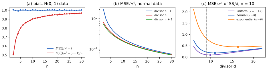
fig_3_s4. Supplementary figure for Wasserman (2004), Theorem 3.17. Download: PDF · SVGThe covariance and correlation measure how strongly two variables move together linearly.
Definition 3.5 (covariance and correlation; Definition 3.18) p. 52, (3.11)–(3.12)
For \(X,Y\) with means \(\mu_X,\mu_Y\) and standard deviations \(\sigma_X,\sigma_Y>0\),
\[ \Cov(X,Y)=\E\big\{(X-\mu_X)(Y-\mu_Y)\big\}, \tag{3.11} \] \[ \rho=\rho_{X,Y}=\rho(X,Y)=\frac{\Cov(X,Y)}{\sigma_X\sigma_Y}. \tag{3.12} \]Result 3.8 (properties of covariance and correlation; Theorem 3.19) p. 52
- \(\Cov(X,Y)=\E(XY)-\E(X)\E(Y)\).
- \(-1\le\rho(X,Y)\le1\).
- If \(Y=aX+b\) with \(a>0\) then \(\rho=1\); with \(a<0\), \(\rho=-1\). Conversely, \(|\rho|=1\) only if \(Y=aX+b\) with probability 1 for some constants \(a\ne0\), \(b\).
- If \(X\) and \(Y\) are independent then \(\Cov(X,Y)=\rho=0\). The converse is false.
Proof (the book gives none)
(1) Expand: \(\E\{XY-\mu_YX-\mu_XY+\mu_X\mu_Y\}\)\({}=\E(XY)-\mu_X\mu_Y\). The product \(XY\) has a mean because \(|xy|\le(x^2+y^2)/2\).
(2) Cauchy–Schwarz. Let \(U=(X-\mu_X)/\sigma_X\) and \(W=(Y-\mu_Y)/\sigma_Y\), standardised variables with \(\E U^2=\E W^2=1\) and \(\E(UW)=\rho\). For every real \(\lambda\),
\[ 0\le\E(W-\lambda U)^2=1-2\lambda\rho+\lambda^2. \]Taking \(\lambda=\rho\) gives \(0\le1-\rho^2\), that is \(|\rho|\le1\).
(3) If \(Y=aX+b\), then \(\mu_Y=a\mu_X+b\), \(\sigma_Y=|a|\sigma_X\), \(\Cov(X,Y)=a\sigma_X^2\) and \(\rho=a/|a|=\sgn(a)\). Conversely, if \(\rho=\pm1\) then with \(\lambda=\rho\) the display gives \(\E(W-\rho U)^2=0\), so \(W=\rho U\) with probability 1 (Result 3.6, applied to the mean-zero variable \(W-\rho U\)). Unwinding the standardisation, \(Y\)\({}=\mu_Y+\rho\frac{\sigma_Y}{\sigma_X}(X-\mu_X)\) with probability 1, a linear function of \(X\) with slope of the sign of \(\rho\).
(4) By Result 3.4, independence gives \(\E(XY)=\E(X)\E(Y)\), so the covariance in (1) is 0. For the converse see the next box. ∎
Filling the gap 3.3: uncorrelated does not mean independent p. 52
Let \(X\sim N(0,1)\) and \(Y=X^2\). Then \(Y\) is a function of \(X\), as dependent as two variables can be, yet \(\Cov(X,Y)\)\({}=\E(X^3)-\E(X)\E(X^2)\)\({}=0-0\)\({}=0\), because the odd moments of a symmetric distribution vanish. Dependence is visible directly: \(\P(|X|>1,\,Y\le1)=0\) while \(\P(|X|>1)\P(Y\le1)\)\({}=0.317\times0.683>0\).
What the correlation does and does not measure
The proof of Result 3.8 shows that \(1-\rho^2\)\({}=\min_\lambda\E(W-\lambda U)^2\) is the mean squared error of the best linear predictor of the standardised \(Y\) from the standardised \(X\). Correlation is therefore a measure of linear association only: \(\rho=0\) says that the best straight line is flat, not that \(X\) carries no information about \(Y\). In the example the best predictor of \(Y\) from \(X\) is \(X^2\) itself, with error 0. Independence is equivalent to \(\Cov(g(X),h(Y))=0\) for all bounded functions \(g,h\) (take indicators \(g=I_A\), \(h=I_B\) to recover \(\P(X\in A,Y\in B)\)\({}=\P(X\in A)\P(Y\in B)\)), a far stronger requirement than one covariance. There is one important case where zero correlation does imply independence: jointly normal variables (Filling the gap 3.7). ∎
Result 3.9 (variance of a sum; Theorem 3.20) p. 52
\(\V(X+Y)=\V(X)+\V(Y)+2\Cov(X,Y)\) and \(\V(X-Y)=\V(X)+\V(Y)-2\Cov(X,Y)\). More generally, for random variables \(X_1,\dots,X_n\) and constants \(a_i\),
\[ \V\Big(\sum_ia_iX_i\Big)=\sum_ia_i^2\V(X_i)+2\sum\!\!\sum_{i<j}a_ia_j\Cov(X_i,X_j). \]Proof (the book gives none)
The covariance is bilinear: \(\Cov(\sum_ia_iX_i,\sum_jb_jY_j)\)\({}=\sum_i\sum_ja_ib_j\Cov(X_i,Y_j)\) (Exercise 3.14). Indeed, centring each variable, \(\sum_ia_iX_i-\E\sum_ia_iX_i\)\({}=\sum_ia_i\tilde X_i\) with \(\tilde X_i=X_i-\E X_i\), and similarly for the \(Y_j\); the product of the two centred sums is \(\sum_i\sum_ja_ib_j\tilde X_i\tilde Y_j\), and linearity of expectation gives the claim. Since \(\V(Z)=\Cov(Z,Z)\), taking \(b=a\) and \(Y=X\),
\[ \V\Big(\sum_ia_iX_i\Big)=\sum_i\sum_ja_ia_j\Cov(X_i,X_j), \]and splitting the double sum into the diagonal \(i=j\) (where \(\Cov(X_i,X_i)=\V(X_i)\)) and the pairs \(i\ne j\), each unordered pair appearing twice by symmetry of the covariance, gives the formula. With \(n=2\), \(a=(1,\pm1)\) it gives the two special cases. ∎
3.4 Expectation and Variance of Important Random Variables
pp. 52–54 The book records the means and variances of the standard distributions in a table, which is reproduced here (the facts are standard) together with derivations of every entry.
| Distribution | Mean | Variance | Derived in |
|---|---|---|---|
| Point mass at \(a\) | \(a\) | \(0\) | Result 3.6 |
| \(\mathrm{Bernoulli}(p)\) | \(p\) | \(p(1-p)\) | Gap 3.4 |
| \(\Bin(n,p)\) | \(np\) | \(np(1-p)\) | Result 3.5 |
| \(\mathrm{Geometric}(p)\) | \(1/p\) | \((1-p)/p^2\) | Gap 3.4 |
| \(\Poi(\lambda)\) | \(\lambda\) | \(\lambda\) | Gap 3.4 |
| \(\mathrm{Uniform}(a,b)\) | \((a+b)/2\) | \((b-a)^2/12\) | Gap 3.5 |
| \(N(\mu,\sigma^2)\) | \(\mu\) | \(\sigma^2\) | Gap 3.5 |
| \(\mathrm{Exponential}(\beta)\) | \(\beta\) | \(\beta^2\) | Gap 3.5 |
| \(\mathrm{Gamma}(\alpha,\beta)\) | \(\alpha\beta\) | \(\alpha\beta^2\) | Gap 3.5 |
| \(\mathrm{Beta}(\alpha,\beta)\) | \(\frac{\alpha}{\alpha+\beta}\) | \(\frac{\alpha\beta}{(\alpha+\beta)^2(\alpha+\beta+1)}\) | Gap 3.5 |
| \(t_\nu\) | \(0\) (if \(\nu>1\)) | \(\frac{\nu}{\nu-2}\) (if \(\nu>2\)) | Gap 3.5 |
| \(\chi^2_p\) | \(p\) | \(2p\) | Gap 3.5 |
| \(\mathrm{Multinomial}(n,\bp)\) | \(n\bp\) | see below | Gap 3.6 |
| \(\mathrm{MVN}(\bmu,\bSigma)\) | \(\bmu\) | \(\bSigma\) | Gap 3.7 |
Every entry was also confirmed numerically against the moments computed by scipy.stats.
See also (companion courses): Result 2.1 (Bernoulli and binomial), Result 2.2 (beta), Result 2.17 (gamma) and Result 2.19 (Student's t) of Bayesian and Probabilistic Machine Learning; Result 3.2 of Foundations of Deep Learning.
Filling the gap 3.4: means and variances of the discrete distributions p. 53, and Exercise 3.12
The Bernoulli, geometric and Poisson rows of the table. The binomial was done in Result 3.5.
Derivations
Bernoulli\((p)\). \(X^2=X\) because \(X\in\{0,1\}\), so \(\E X=\E X^2=p\) and \(\V X=p-p^2=p(1-p)\).
Geometric\((p)\), \(f(k)=p(1-p)^{k-1}\) for \(k=1,2,\dots\) (the number of the toss on which the first head appears). Write \(q=1-p\). Differentiating the geometric series \(\sum_{k\ge0}s^k=1/(1-s)\) term by term inside its radius of convergence \(|s|<1\) gives \(\sum_{k\ge1}ks^{k-1}=(1-s)^{-2}\) and \(\sum_{k\ge2}k(k-1)s^{k-2}\)\({}=2(1-s)^{-3}\). Hence
\[ \E X=p\sum_{k\ge1}kq^{k-1}=\frac p{p^2}=\frac1p, \] \[ \E\{X(X-1)\}=pq\sum_{k\ge2}k(k-1)q^{k-2}=\frac{2pq}{p^3}=\frac{2q}{p^2}. \]So \(\V X\)\({}=\E\{X(X-1)\}+\E X-(\E X)^2\)\({}=\frac{2q}{p^2}+\frac1p-\frac1{p^2}\)\({}=\frac{q}{p^2}\)\({}=\frac{1-p}{p^2}\). (A slicker route: conditioning on the first toss, \(\E X=1+q\E X\), the rule of iterated expectations of Result 3.11.)
Poisson\((\lambda)\), \(f(k)=e^{-\lambda}\lambda^k/k!\). Using \(\sum_{j\ge0}\lambda^j/j!\)\({}=e^\lambda\) and shifting the index,
\[ \E X=\sum_{k\ge1}k\,e^{-\lambda}\frac{\lambda^k}{k!}=\lambda e^{-\lambda}\sum_{k\ge1}\frac{\lambda^{k-1}}{(k-1)!}=\lambda, \] \[ \E\{X(X-1)\}=\lambda^2e^{-\lambda}\sum_{k\ge2}\frac{\lambda^{k-2}}{(k-2)!}=\lambda^2. \]So \(\V X\)\({}=\lambda^2+\lambda-\lambda^2\)\({}=\lambda\). The factorial moment \(\E\{X(X-1)\}\) is the natural intermediate step for distributions with factorials in the mass function, as the book's hint says. ∎
Filling the gap 3.5: means and variances of the continuous distributions p. 53, and Exercise 3.12
The uniform, normal, exponential, gamma, beta, \(t\) and \(\chi^2\) rows. The device throughout: an integral that looks new is often a known density with different parameters, times a constant.
Derivations
Uniform\((a,b)\). \(\E X\)\({}=\frac1{b-a}\int_a^bx\,\d x\)\({}=\frac{a+b}2\) and \(\E X^2\)\({}=\frac{b^3-a^3}{3(b-a)}\)\({}=\frac{a^2+ab+b^2}3\), so \(\V X\)\({}=\frac{a^2+ab+b^2}3-\frac{(a+b)^2}4\)\({}=\frac{(b-a)^2}{12}\).
Normal. If \(Z\sim N(0,1)\), \(\E Z=0\) because \(z\phi(z)\) is odd and integrable, and integrating by parts with \(\phi'(z)=-z\phi(z)\), \(\E Z^2\)\({}=\int z\cdot z\phi(z)\,\d z\)\({}=[-z\phi(z)]_{-\infty}^\infty+\int\phi(z)\,\d z\)\({}=1\). For \(X\)\({}=\mu+\sigma Z\sim N(\mu,\sigma^2)\), Result 3.5 gives \(\E X=\mu\) and \(\V X=\sigma^2\).
Gamma\((\alpha,\beta)\), density \(x^{\alpha-1}e^{-x/\beta}/\{\Gamma(\alpha)\beta^\alpha\}\) on \(x>0\). For any \(k>-\alpha\), the integrand of \(\E X^k\) is a Gamma\((\alpha+k,\beta)\) density up to its constant:
\[ \begin{aligned}\E X^k&=\frac1{\Gamma(\alpha)\beta^\alpha}\int_0^\infty x^{\alpha+k-1}e^{-x/\beta}\,\d x\\&=\frac{\Gamma(\alpha+k)\beta^{\alpha+k}}{\Gamma(\alpha)\beta^\alpha}\\&=\beta^k\frac{\Gamma(\alpha+k)}{\Gamma(\alpha)}.\end{aligned} \]With \(\Gamma(\alpha+1)\)\({}=\alpha\Gamma(\alpha)\): \(\E X=\alpha\beta\), \(\E X^2=\alpha(\alpha+1)\beta^2\), so \(\V X=\alpha\beta^2\). The exponential\((\beta)\) is Gamma\((1,\beta)\): mean \(\beta\), variance \(\beta^2\). The \(\chi^2_p\) is Gamma\((p/2,2)\): mean \(p\), variance \(2p\).
Beta\((\alpha,\beta)\), density \(x^{\alpha-1}(1-x)^{\beta-1}/B(\alpha,\beta)\) on \((0,1)\), \(B(\alpha,\beta)\)\({}=\Gamma(\alpha)\Gamma(\beta)/\Gamma(\alpha+\beta)\). In the same way
\[ \begin{aligned}\E X^k&=\frac{B(\alpha+k,\beta)}{B(\alpha,\beta)}\\&=\frac{\Gamma(\alpha+k)\Gamma(\alpha+\beta)}{\Gamma(\alpha)\Gamma(\alpha+\beta+k)},\end{aligned} \]so \(\E X=\frac\alpha{\alpha+\beta}\), \(\E X^2\)\({}=\frac{\alpha(\alpha+1)}{(\alpha+\beta)(\alpha+\beta+1)}\) and
\[ \begin{aligned}\V X&=\frac{\alpha(\alpha+1)}{(\alpha+\beta)(\alpha+\beta+1)}-\frac{\alpha^2}{(\alpha+\beta)^2}\\&=\frac{\alpha\beta}{(\alpha+\beta)^2(\alpha+\beta+1)}.\end{aligned} \]Student's \(t_\nu\). Represent \(T=Z/\sqrt{V/\nu}\) with \(Z\sim N(0,1)\) independent of \(V\sim\chi^2_\nu\). The density of \(T\) behaves like \(|t|^{-(\nu+1)}\) in the tails, so \(\E|T|^k<\infty\) exactly when \(k<\nu\): the mean exists only for \(\nu>1\) (\(\nu=1\) is the Cauchy) and the variance only for \(\nu>2\). When they exist, independence and Result 3.4 give \(\E T=\E Z\,\E\sqrt{\nu/V}=0\) and
\[ \begin{aligned}\E T^2&=\nu\,\E Z^2\,\E V^{-1}\\&=\nu\cdot\frac{\Gamma(\nu/2-1)}{2\Gamma(\nu/2)}\\&=\frac{\nu}{\nu-2},\end{aligned} \]using the gamma moment above with \(k=-1\), \(\alpha=\nu/2\), \(\beta=2\) (valid for \(\nu/2>1\)). ∎
The last two rows of the table concern random vectors.
Definition 3.6 (mean vector and covariance matrix) p. 53
For a random vector \(\bX=(X_1,\dots,X_k)^\T\), the mean is the vector \(\bmu\)\({}=\E(\bX)\)\({}=(\E X_1,\dots,\E X_k)^\T\), and the variance–covariance matrix is the \(k\times k\) matrix \(\bSigma=\V(\bX)\) with entries \(\Sigma_{ij}=\Cov(X_i,X_j)\); its diagonal holds the variances \(\V(X_i)\). In matrix form, \(\bSigma\)\({}=\E\{(\bX-\bmu)(\bX-\bmu)^\T\}\), the expectation of a matrix being taken entry by entry.
Result 3.10 (linear combinations of random vectors; Lemma 3.21) p. 54
Let \(\bX\) have mean \(\bmu\) and covariance matrix \(\bSigma\). For a fixed vector \(\ba\), \(\E(\ba^\T\bX)=\ba^\T\bmu\) and \(\V(\ba^\T\bX)=\ba^\T\bSigma\ba\). For a fixed \(m\times k\) matrix \(\bA\), \(\E(\bA\bX)=\bA\bmu\) and \(\V(\bA\bX)=\bA\bSigma\bA^\T\). Consequently \(\bSigma\) is symmetric and positive semi-definite.
Proof (the book leaves it as Exercise 3.20)
Row \(i\) of \(\bA\bX\) is \(\sum_jA_{ij}X_j\), whose mean is \(\sum_jA_{ij}\mu_j\) by linearity: \(\E(\bA\bX)=\bA\bmu\). For the covariance, \(\bA\bX-\bA\bmu=\bA(\bX-\bmu)\), so
\[ \begin{aligned}\V(\bA\bX)&=\E\{\bA(\bX-\bmu)(\bX-\bmu)^\T\bA^\T\}\\&=\bA\,\E\{(\bX-\bmu)(\bX-\bmu)^\T\}\,\bA^\T\\&=\bA\bSigma\bA^\T,\end{aligned} \]where taking the fixed matrices outside the expectation is linearity applied entry by entry: entry \((i,l)\) of the middle expression is \(\sum_{j,m}A_{ij}A_{lm}\E\{(X_j-\mu_j)(X_m-\mu_m)\}\). The vector case is \(\bA=\ba^\T\) (one row). Symmetry of \(\bSigma\) is the symmetry of the covariance. Positive semi-definiteness: \(\ba^\T\bSigma\ba\)\({}=\V(\ba^\T\bX)\ge0\) for every \(\ba\). It is singular exactly when some non-trivial combination \(\ba^\T\bX\) has variance 0, that is (Result 3.6) when the vector lies with probability 1 in a hyperplane. ∎
Filling the gap 3.6: the multinomial covariance matrix, directly pp. 53–54
For \(\bX\sim\mathrm{Multinomial}(n,\bp)\), \(\E\bX=n\bp\) and \(\V(\bX)=n\{\diag(\bp)-\bp\bp^\T\}\): \(\V(X_i)=np_i(1-p_i)\) and \(\Cov(X_i,X_j)=-np_ip_j\) for \(i\ne j\). The book gets the covariance by matching two expressions for \(\V(X_i+X_j)\); here is a second derivation that also shows why the matrix is singular.
Proof
Write \(\bX=\sum_{t=1}^n\bY_t\), where \(\bY_t\) is the indicator vector of the category of draw \(t\): exactly one entry is 1, the one equal to \(j\) with probability \(p_j\). The \(\bY_t\) are independent, so by Result 3.9 (covariances of independent vectors vanish) \(\V(\bX)=n\V(\bY_1)\). For one draw, \(\E Y_{1i}=p_i\); \(Y_{1i}^2=Y_{1i}\) gives \(\V(Y_{1i})=p_i-p_i^2\); and \(Y_{1i}Y_{1j}=0\) for \(i\ne j\) (one draw falls in one category) gives \(\Cov(Y_{1i},Y_{1j})=0-p_ip_j\). So \(\V(\bY_1)=\diag(\bp)-\bp\bp^\T\). The negative covariance has a plain meaning: the counts compete for the same \(n\) draws. The matrix is singular because \(\sum_iX_i=n\) is constant: with \(\mathbf1=(1,\dots,1)^\T\), \(\mathbf1^\T\V(\bX)\mathbf1\)\({}=\V(\sum_iX_i)\)\({}=0\). ∎
See also (companion courses): Result 2.5 of Bayesian and Probabilistic Machine Learning and Result 3.3 of Foundations of Deep Learning.
Filling the gap 3.7: the multivariate normal, its mean and covariance, and linear maps p. 53 (table) and Chapter 2
Let \(\bZ=(Z_1,\dots,Z_k)^\T\) have independent \(N(0,1)\) entries, let \(\bmu\in\R^k\), and let \(\bSigma\) be a symmetric positive definite \(k\times k\) matrix with symmetric square root \(\bSigma^{1/2}\). The vector \(\bX=\bmu+\bSigma^{1/2}\bZ\) has the \(N(\bmu,\bSigma)\) density of Chapter 2,
\[ f(\mathbf x)=\frac1{(2\pi)^{k/2}|\bSigma|^{1/2}}\exp\Big\{-\tfrac12(\mathbf x-\bmu)^\T\bSigma^{-1}(\mathbf x-\bmu)\Big\}, \]and then:
- \(\E\bX=\bmu\) and \(\V(\bX)=\bSigma\): the parameters are the mean vector and the covariance matrix;
- its moment generating function is \(\E e^{\bt^\T\bX}\)\({}=\exp(\bt^\T\bmu+\tfrac12\bt^\T\bSigma\bt)\) for all \(\bt\in\R^k\);
- for any fixed \(m\times k\) matrix \(\bA\) and \(\bb\in\R^m\), \(\bA\bX+\bb\sim N(\bA\bmu+\bb,\bA\bSigma\bA^\T)\) (a normal vector, degenerate if \(\bA\bSigma\bA^\T\) is singular); in particular every linear combination \(\ba^\T\bX\) is \(N(\ba^\T\bmu,\ba^\T\bSigma\ba)\), and every sub-vector is normal;
- \(\bSigma^{-1/2}(\bX-\bmu)\sim N(\mathbf0,\bI)\), and \((\bX-\bmu)^\T\bSigma^{-1}(\bX-\bmu)\sim\chi^2_k\);
- components of \(\bX\) that are uncorrelated are independent.
Proof
The density. \(\bZ\) has density \((2\pi)^{-k/2}e^{-\mathbf z^\T\mathbf z/2}\). The map \(\mathbf z\mapsto\bmu+\bSigma^{1/2}\mathbf z\) is invertible with inverse \(\mathbf z\)\({}=\bSigma^{-1/2}(\mathbf x-\bmu)\) and Jacobian determinant \(|\bSigma|^{-1/2}\), and \(\mathbf z^\T\mathbf z\)\({}=(\mathbf x-\bmu)^\T\bSigma^{-1}(\mathbf x-\bmu)\); the change-of-variables formula gives \(f\).
(1) \(\E\bZ=\mathbf0\) and \(\V(\bZ)=\bI\) (independent unit variances). By Result 3.10, \(\E\bX=\bmu\) and \(\V(\bX)\)\({}=\bSigma^{1/2}\bI\bSigma^{1/2}\)\({}=\bSigma\).
(2) For one standard normal, completing the square gives \(\E e^{sZ}\)\({}=\int e^{sz-z^2/2}\,\d z/\sqrt{2\pi}\)\({}=e^{s^2/2}\int e^{-(z-s)^2/2}\,\d z/\sqrt{2\pi}\)\({}=e^{s^2/2}\). With \(\mathbf s=\bSigma^{1/2}\bt\), independence of the \(Z_i\) and Result 3.4, \(\E e^{\mathbf s^\T\bZ}\)\({}=\prod_ie^{s_i^2/2}\)\({}=e^{\mathbf s^\T\mathbf s/2}\)\({}=e^{\bt^\T\bSigma\bt/2}\), and \(\E e^{\bt^\T\bX}\)\({}=e^{\bt^\T\bmu}\E e^{\mathbf s^\T\bZ}\).
(3) For \(\bY=\bA\bX+\bb\) and \(\mathbf u\in\R^m\), \(\E e^{\mathbf u^\T\bY}\)\({}=e^{\mathbf u^\T\bb}\E e^{(\bA^\T\mathbf u)^\T\bX}\)\({}=\exp\{\mathbf u^\T(\bA\bmu+\bb)+\tfrac12\mathbf u^\T\bA\bSigma\bA^\T\mathbf u\}\), the mgf of \(N(\bA\bmu+\bb,\bA\bSigma\bA^\T)\). The multivariate version of the uniqueness theorem (Result 3.14) identifies the distribution. Sub-vectors are the case where \(\bA\) selects coordinates.
(4) \(\bSigma^{-1/2}(\bX-\bmu)=\bZ\), and \(\bZ^\T\bZ=\sum Z_i^2\) is a sum of \(k\) independent squared standard normals, which is \(\chi^2_k\) by definition (Chapter 2).
(5) Split \(\bX=(\bX_1,\bX_2)\) with \(\Cov(\bX_1,\bX_2)=\mathbf0\), so \(\bSigma\) is block diagonal. Then \(\bt^\T\bSigma\bt\)\({}=\bt_1^\T\bSigma_{11}\bt_1+\bt_2^\T\bSigma_{22}\bt_2\) and the joint mgf factorises into the mgfs of \(\bX_1\) and \(\bX_2\); it is therefore the mgf of a pair of independent normal vectors with those marginals, and uniqueness gives independence. For a general (not jointly normal) pair this fails, as Filling the gap 3.3 shows. ∎
See also (companion courses): the mean and covariance of the Gaussian by direct integration in Result 3.5 of Foundations of Deep Learning and Result 2.7 of Bayesian and Probabilistic Machine Learning, with the linear algebra in Filling the gap 2.2 there.
3.5 Conditional Expectation
pp. 54–56 What is the mean of \(X\) among the occasions on which \(Y=y\)? Compute the mean as before, with the conditional distribution of \(X\) given \(Y=y\) in place of the distribution of \(X\).
See also (companion courses): Result 2.4 of Bayesian and Probabilistic Machine Learning (conditional expectation and variance; Bayesian learning reduces uncertainty on average) and Exercise 2.11 of Foundations of Deep Learning.
Definition 3.7 (conditional expectation; Definition 3.22) p. 54, (3.13)–(3.14)
The conditional expectation of \(X\) given \(Y=y\) is
\[ \E(X\given Y=y)=\begin{cases}\sum_xx\,f_{X|Y}(x\given y)&\text{discrete case,}\\[2pt]\int x\,f_{X|Y}(x\given y)\,\d x&\text{continuous case.}\end{cases} \tag{3.13} \]For a function \(r(x,y)\),
\[ \E\big(r(X,Y)\given Y=y\big)=\begin{cases}\sum_xr(x,y)\,f_{X|Y}(x\given y)&\text{discrete case,}\\[2pt]\int r(x,y)\,f_{X|Y}(x\given y)\,\d x&\text{continuous case.}\end{cases} \tag{3.14} \]The number \(\E(X\given Y=y)\) is a function of \(y\), say \(m(y)\). Evaluated at the random \(Y\) it gives a random variable, written \(\E(X\given Y)=m(Y)\): its value is \(\E(X\given Y=y)\) when \(Y=y\). Likewise \(\E(r(X,Y)\given Y)\).
(The book prints a stray "\(\d x\)" after the discrete sums; it is listed in the author's errata.) In Example 3.23, \(X\sim\Unif(0,1)\) and, given \(X=x\), \(Y\sim\Unif(x,1)\): the conditional density is \(1/(1-x)\) on \((x,1)\), and \(\E(Y\given X=x)\)\({}=\frac1{1-x}\int_x^1y\,\d y\)\({}=\frac{1+x}2\), the midpoint of the interval, as intuition says. So \(\E(Y\given X)=(1+X)/2\), a random variable uniform on \((\tfrac12,1)\). Figure 3.S5(a) shows the line \(x\mapsto(1+x)/2\) through a cloud of simulated pairs.
Filling the gap 3.8: working with \(\E(Y\given X)\) as a random variable pp. 54–56, and Exercises 3.16, 3.18
Let \(m(x)=\E(Y\given X=x)\) and assume \(\E|Y|<\infty\). Then, with probability 1:
- Linearity: \(\E(aY_1+bY_2\given X)\)\({}=a\E(Y_1\given X)+b\E(Y_2\given X)\).
- Taking out what is known: \(\E\{r(X)s(Y)\given X\}\)\({}=r(X)\,\E\{s(Y)\given X\}\), and in particular \(\E\{r(X)\given X\}=r(X)\) (Exercise 3.16).
- Independence: if \(X\) and \(Y\) are independent, \(\E(Y\given X)=\E(Y)\), a constant.
- Orthogonality: \(\E\{(Y-m(X))\,g(X)\}=0\) for every \(g\) with \(\E\{g(X)^2\}<\infty\) (when \(\E Y^2<\infty\)).
- Best predictor: among all functions \(g\), \(\E\{(Y-g(X))^2\}\) is smallest for \(g=m\), and \(\E\{(Y-g(X))^2\}\) equals \(\E\{(Y-m(X))^2\}\)\({}+\E\{(m(X)-g(X))^2\}\).
- If \(\E(Y\given X=x)=c\) for every \(x\), then \(\Cov(X,Y)=0\) (Exercise 3.18, with the roles of the letters swapped).
Proof
(1) is linearity of the sum or integral in (3.14) for each fixed \(x\). (2) For fixed \(x\), \(\E\{r(X)s(Y)\given X\)\({}=x\}\)\({}=\int r(x)s(y)f(y\given x)\,\d y\)\({}=r(x)\int s(y)f(y\given x)\,\d y\): given \(X=x\), \(r(X)\) is the constant \(r(x)\). Taking \(s\equiv1\) gives \(\E\{r(X)\given X\}=r(X)\). (3) Independence means \(f(y\given x)=f_Y(y)\), so \(m(x)=\E Y\) for every \(x\).
(4) By the rule of iterated expectations (Result 3.11, which does not use this box) and (2), \(\E\{Yg(X)\}\)\({}=\E[\E\{Yg(X)\given X\}]\)\({}=\E\{g(X)m(X)\}\), so \(\E\{(Y-m(X))g(X)\}=0\).
(5) Write \(Y-g(X)\)\({}=(Y-m(X))\)\({}+(m(X)-g(X))\) and expand the square; the cross term is \(2\E\{(Y-m(X))(m(X)-g(X))\}=0\) by (4) with the function \(m-g\). Both remaining terms are non-negative and only the second depends on \(g\); it vanishes for \(g=m\). This is why the regression function \(m(x)\) is the target of prediction under squared error (Chapter 13 of the book).
(6) By iterated expectations \(\E Y=\E\,m(X)=c\), and \(\E(XY)=\E\{X\,m(X)\}=c\,\E X\) by (2), so \(\Cov(X,Y)=c\E X-\E X\cdot c=0\). The converse fails: uncorrelated variables can have a non-constant conditional mean (in Filling the gap 3.3, \(\E(X^2\given X)=X^2\)).
A word on rigour. For a continuous \(X\) the event \(\{X=x\}\) has probability 0, so \(f(y\given x)=f(x,y)/f_X(x)\) is only defined where \(f_X(x)>0\), and changing the density on a set of probability 0 changes \(m\) there. The random variable \(m(X)\) is therefore defined up to an event of probability 0, which is why the statements above hold "with probability 1". Measure-theoretic probability defines \(\E(Y\given X)\) directly as the (almost surely unique) function of \(X\) satisfying the orthogonality (4) with all bounded \(g\), and everything here follows from that definition. ∎
See also (companion course): the regression function is the conditional mean, Result 1.18 of Bayesian and Probabilistic Machine Learning.
Result 3.11 (the rule of iterated expectations; Theorem 3.24) p. 55, (3.15)–(3.16)
For random variables \(X\) and \(Y\) whose expectations exist,
\[ \E\big[\E(Y\given X)\big]=\E(Y)\quad\text{and}\quad\E\big[\E(X\given Y)\big]=\E(X). \tag{3.15} \]More generally, for any \(r(x,y)\) with \(\E|r(X,Y)|<\infty\),
\[ \E\big[\E\big(r(X,Y)\given X\big)\big]=\E\big(r(X,Y)\big). \tag{3.16} \]Proof
It is enough to prove (3.16); (3.15) is the case \(r(x,y)=y\) (and, swapping the names, \(r(x,y)=x\) conditioned on \(Y\)). Let \(g(x)\)\({}=\E(r(X,Y)\given X=x)\)\({}=\int r(x,y)f(y\given x)\,\d y\). By the rule of the lazy statistician and the factorisation \(f(x,y)=f_X(x)f(y\given x)\),
\[ \begin{aligned}\E\,g(X)&=\int\Big\{\int r(x,y)f(y\given x)\,\d y\Big\}f_X(x)\,\d x\\&=\iint r(x,y)f(x,y)\,\d y\,\d x\\&=\E\,r(X,Y).\end{aligned} \]The exchange of the order of integration hidden in the middle step is justified by Fubini's theorem, because \(\iint|r(x,y)|f(x,y)\,\d y\,\d x\)\({}=\E|r(X,Y)|<\infty\). The discrete case is identical with sums. The book proves the first identity in (3.15) the same way. ∎
Example 3.25 shows the rule's use: in Example 3.23, \(\E(Y)\)\({}=\E\{(1+X)/2\}\)\({}=(1+\tfrac12)/2\)\({}=\tfrac34\), without the joint density.
Definition 3.8 (conditional variance; Definition 3.26) p. 55, (3.17)
\[ \V(Y\given X=x)=\int\big(y-\mu(x)\big)^2f(y\given x)\,\d y,\qquad\mu(x)=\E(Y\given X=x). \tag{3.17} \]As with the conditional mean, \(\V(Y\given X)\) is the random variable whose value is \(\V(Y\given X=x)\) when \(X=x\). By the argument of Result 3.5 applied to the conditional distribution, \(\V(Y\given X)\)\({}=\E(Y^2\given X)-\{\E(Y\given X)\}^2\).
Result 3.12 (the law of total variance; Theorem 3.27) p. 55
For random variables \(X\) and \(Y\) with \(\E Y^2<\infty\),
\[ \V(Y)=\E\,\V(Y\given X)+\V\,\E(Y\given X). \]The first term is the average spread of \(Y\) around its conditional mean; the second is the spread of the conditional mean itself.
Proof (the book leaves it as Exercise 3.17)
Let \(m=\E(Y)\) and \(b(x)=\E(Y\given X=x)\). By Result 3.11, \(\E\,b(X)=m\). Write \(Y-m=(Y-b(X))+(b(X)-m)\) and expand:
\[ \V(Y)=\E(Y-b(X))^2+2\E\{(Y-b(X))(b(X)-m)\}+\E(b(X)-m)^2. \]Each term is computed by iterated expectations, \(\E(\cdot)=\E\{\E(\cdot\given X)\}\):
- \(\E\{(Y-b(X))^2\given X\}\)\({}=\V(Y\given X)\) by Definition 3.8, so the first term is \(\E\,\V(Y\given X)\);
- given \(X\), the factor \(b(X)-m\) is known and \(\E\{Y-b(X)\given X\}=b(X)-b(X)=0\) (Filling the gap 3.8, part 2), so the cross term is 0;
- \(b(X)\) has mean \(m\), so the last term is \(\V\{b(X)\}=\V\,\E(Y\given X)\).
All three expectations are finite because \(\E Y^2<\infty\) and \(\E\,b(X)^2\le\E\,\E(Y^2\given X)\)\({}=\E Y^2\) (the conditional version of \(\{\E W\}^2\le\E W^2\)). ∎
The decomposition is an analysis of variance: total variation = within-group variation + between-group variation. For the two-stage experiment of Example 3.23, \(\V(Y\given X)=(1-X)^2/12\) (a uniform on an interval of length \(1-X\)) and \(\E(Y\given X)=(1+X)/2\), so \(\V(Y)\)\({}=\E(1-X)^2/12+\V(X)/4\)\({}=\tfrac1{36}+\tfrac1{48}\)\({}=\tfrac7{144}\).
Example 3.28 is a hierarchical model: draw a county at random, with an unknown disease proportion \(Q\sim\Unif(0,1)\), then sample \(n\) people from it, \(X\given Q=q\sim\Bin(n,q)\). Then \(\E(X)=\E(nQ)=n/2\) and
\[ \V(X)=\E\{nQ(1-Q)\}+\V(nQ)=n\int_0^1q(1-q)\,\d q+n^2\V(Q)=\frac n6+\frac{n^2}{12}. \]The second term grows like \(n^2\): when counties differ, sampling more people per county does not average the difference away. (Strictly, sampling people without replacement from a finite county gives a hypergeometric count; the binomial is the large-county approximation.)
Filling the gap 3.9: in Example 3.28, \(X\) is exactly uniform on \(\{0,\dots,n\}\) p. 56
With \(Q\sim\Unif(0,1)\) the count is uniform: \(\P(X=k)=1/(n+1)\) for \(k=0,\dots,n\). More generally, with \(Q\sim\mathrm{Beta}(\alpha,\beta)\) the count has the beta-binomial distribution, with
\[ \E X=\frac{n\alpha}{\alpha+\beta},\qquad\V X=n\,\frac{\alpha}{\alpha+\beta}\,\frac{\beta}{\alpha+\beta}\cdot\frac{\alpha+\beta+n}{\alpha+\beta+1}. \]The last factor, larger than 1 for \(n>1\), is the overdispersion relative to a binomial with the same mean.
Proof
Averaging the binomial probability over \(Q\) (the law of total probability for a continuous first stage) and using the beta integral \(\int_0^1q^{a-1}(1-q)^{b-1}\,\d q\)\({}=\Gamma(a)\Gamma(b)/\Gamma(a+b)\),
\[ \P(X=k)=\int_0^1\binom nkq^k(1-q)^{n-k}\,\d q=\binom nk\frac{k!\,(n-k)!}{(n+1)!}=\frac1{n+1}. \]The uniform distribution on \(\{0,\dots,n\}\) has variance \(\{(n+1)^2-1\}/12=(n^2+2n)/12\), which is \(n/6+n^2/12\), as the law of total variance said. For the beta case, write \(\mu_Q=\alpha/(\alpha+\beta)\) and use \(\V(Q)\)\({}=\mu_Q(1-\mu_Q)/(\alpha+\beta+1)\) from Filling the gap 3.5. Then \(\E\,\V(X\given Q)\)\({}=n\{\mu_Q(1-\mu_Q)-\V(Q)\}\) and \(\V\,\E(X\given Q)=n^2\V(Q)\), so
\[ \V X=n\mu_Q(1-\mu_Q)+n(n-1)\V(Q)=n\mu_Q(1-\mu_Q)\Big(1+\frac{n-1}{\alpha+\beta+1}\Big), \]which is the formula. With \(\alpha=\beta=1\) it gives \(n(n+2)/12\) again. ∎
See also (companion course): the beta-binomial and its overdispersion in Statistical Methods for Modern Biology, Filling the gap 2.15.
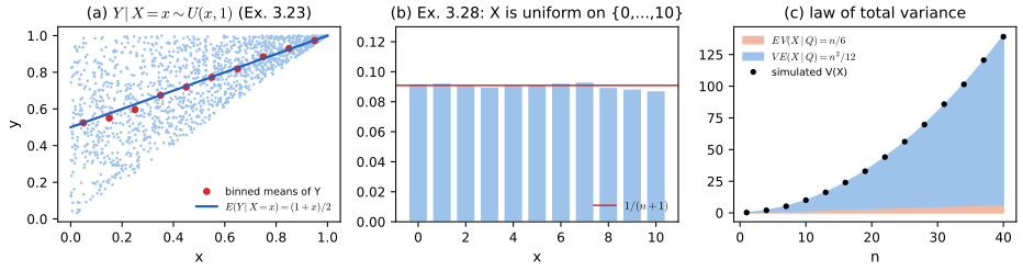
fig_3_s5. Supplementary figure for Wasserman (2004), Examples 3.23, 3.25 and 3.28. Download: PDF · SVG3.6 Moment Generating Functions
pp. 56–58 The moment generating function packs all the moments of a distribution into one function. It is used to compute moments, to find the distribution of sums of independent variables, and in proofs such as that of the central limit theorem (Chapter 5).
See also: the first-year notes Moment generating functions and the normal family.
Definition 3.9 (moment generating function; Definition 3.29) p. 56
The moment generating function (mgf) of \(X\) is
\[ \psi_X(t)=\E\big(e^{tX}\big)=\int e^{tx}\,\d F(x),\qquad t\in\R. \]It is always defined at \(t=0\) (\(\psi_X(0)=1\)) and may be \(+\infty\) elsewhere. As in the book, we assume from now on that \(\psi_X(t)<\infty\) for all \(t\) in an open interval \((-h,h)\), \(h>0\).
Two remarks on the definition. The book also calls \(\psi_X\) the Laplace transform; strictly, the (two-sided) Laplace transform of the distribution is \(\E e^{-sX}\), so \(\psi_X(t)\) is that transform evaluated at \(s=-t\). The characteristic function \(\E e^{itX}\), \(i=\sqrt{-1}\), is the same expression on the imaginary axis; because \(|e^{itX}|=1\) it exists for every distribution and every \(t\), which is why the general theory uses it.
Filling the gap 3.10: why we may differentiate under the expectation, and the moment series pp. 56–57
If \(\psi_X(t)<\infty\) for \(|t|<h\), then every moment \(\E|X|^k\) is finite, and for \(|t|<h\)
\[ \psi_X(t)=\sum_{k=0}^\infty\frac{\E(X^k)}{k!}t^k, \qquad\text{so}\qquad \psi_X^{(k)}(0)=\E(X^k)\ \text{ for every }k. \]The book asserts that "it can be shown" that differentiation and expectation may be exchanged; this is the proof.
Proof
A two-sided bound. Fix \(0<s<h\). For every real \(x\), \(e^{s|x|}\le e^{sx}+e^{-sx}\), so \(\E e^{s|X|}\le\psi_X(s)+\psi_X(-s)<\infty\).
All moments are finite. Since \(e^{s|x|}=\sum_k(s|x|)^k/k!\) has non-negative terms, \(\frac{s^k|x|^k}{k!}\le e^{s|x|}\), so \(\E|X|^k\le k!\,s^{-k}\E e^{s|X|}<\infty\).
The series. For \(|t|\le s\), the series \(\sum_kt^kX^k/k!\) converges to \(e^{tX}\) and is dominated term by term in absolute value by the series of \(e^{s|X|}\), whose expectation is finite. By Tonelli's theorem \(\sum_k|t|^k\E|X|^k/k!\)\({}=\E e^{|t||X|}<\infty\), so Fubini's theorem (or dominated convergence for the partial sums) allows expectation and summation to be exchanged: \(\psi_X(t)=\sum_k\E(X^k)t^k/k!\) for \(|t|\le s\), and since \(s<h\) was arbitrary, for \(|t|<h\).
Derivatives. A power series may be differentiated term by term inside its interval of convergence, and the \(k\)th derivative at 0 picks out \(k!\) times the \(k\)th coefficient: \(\psi_X^{(k)}(0)=\E(X^k)\). Equivalently, \(\psi_X^{(k)}(t)=\E(X^ke^{tX})\) for \(|t|<h\): differentiation under \(\E\) is allowed because the difference quotients are dominated by \(|X|^ke^{s|X|}\cdot\)const, which is integrable.
When the assumption fails. If \(\psi_X\) is finite only at \(t=0\) (the Cauchy, or the \(t\) distributions) or only on one side of 0 (the lognormal, whose mgf is infinite for every \(t>0\) although all its moments are finite), the expansion and the uniqueness theorem below are not available. ∎
The cumulant generating function \(K(t)=\log\psi_X(t)\) is often handier: from \(K'=\psi'/\psi\) and \(K''=\psi''/\psi-(\psi'/\psi)^2\), \(K'(0)=\E X\) and \(K''(0)=\E X^2-(\E X)^2=\V X\). The demonstration plots \(K\) for this reason.
Example 3.30: for \(X\sim\mathrm{Exp}(1)\), \(\psi_X(t)\)\({}=\int_0^\infty e^{(t-1)x}\,\d x\)\({}=1/(1-t)\) for \(t<1\), and the integral diverges for \(t\ge1\). Then \(\psi'(t)=(1-t)^{-2}\) and \(\psi''(t)=2(1-t)^{-3}\), so \(\E X=1\), \(\E X^2=2\) and \(\V X=1\). In fact \(1/(1-t)=\sum_kt^k\), so \(\E X^k=k!\) (Figure 3.S6(a)).
Result 3.13 (properties of the mgf; Lemma 3.31) p. 57
- If \(Y=aX+b\), then \(\psi_Y(t)=e^{bt}\psi_X(at)\).
- If \(X_1,\dots,X_n\) are independent and \(Y=\sum_iX_i\), then \(\psi_Y(t)=\prod_i\psi_i(t)\), where \(\psi_i\) is the mgf of \(X_i\).
Proof (the book gives none)
(1) \(e^{tY}=e^{bt}e^{(at)X}\), and \(e^{bt}\) is a constant. (2) \(e^{tY}=\prod_ie^{tX_i}\), and the factors \(e^{tX_i}\) are independent non-negative random variables; the product rule (Result 3.4, in the form for functions of independent variables, which holds for non-negative variables even when some expectations are infinite, by Tonelli's theorem) gives \(\E e^{tY}=\prod_i\E e^{tX_i}\). In particular \(\psi_Y\) is finite near 0 when every \(\psi_i\) is. ∎
Example 3.32: a Bernoulli variable has \(\psi(t)=pe^t+q\) with \(q=1-p\), so \(X\sim\Bin(n,p)\), a sum of \(n\) independent Bernoulli variables, has \(\psi_X(t)=(pe^t+q)^n\). Differentiating, \(\psi_X'(0)=np\) and \(\psi_X''(0)=n(n-1)p^2+np\), which give the mean \(np\) and variance \(np(1-p)\) once more.
Filling the gap 3.11: the table of moment generating functions p. 58, and Exercise 3.23
\[ \begin{array}{ll}\text{Bernoulli}(p)&pe^t+(1-p)\\ \Bin(n,p)&\big(pe^t+(1-p)\big)^n\\ \Poi(\lambda)&e^{\lambda(e^t-1)}\\ N(\mu,\sigma^2)&\exp\big(\mu t+\sigma^2t^2/2\big)\\ \mathrm{Gamma}(\alpha,\beta)&(1-\beta t)^{-\alpha},\ t<1/\beta\end{array} \](The book's table labels the normal row "Normal\((\mu,\sigma)\)"; the formula is the one for variance \(\sigma^2\), the parametrisation used everywhere else in the book.)
Derivations
Bernoulli, binomial: above. Poisson: \(\E e^{tX}\)\({}=\sum_ke^{tk}e^{-\lambda}\lambda^k/k!\)\({}=e^{-\lambda}\sum_k(\lambda e^t)^k/k!\)\({}=e^{-\lambda}e^{\lambda e^t}\), finite for every \(t\). Normal: for \(Z\sim N(0,1)\), completing the square in the exponent, \(tz-z^2/2=t^2/2-(z-t)^2/2\), gives \(\E e^{tZ}\)\({}=e^{t^2/2}\int\phi(z-t)\,\d z\)\({}=e^{t^2/2}\); then \(X=\mu+\sigma Z\) and Result 3.13(1) give \(e^{\mu t}e^{\sigma^2t^2/2}\). Gamma: for \(t<1/\beta\), with \(1/\beta'=1/\beta-t\), i.e. \(\beta'=\beta/(1-\beta t)\),
\[ \begin{aligned}\E e^{tX}&=\frac1{\Gamma(\alpha)\beta^\alpha}\int_0^\infty x^{\alpha-1}e^{-x/\beta'}\,\d x\\&=\frac{\Gamma(\alpha)\beta'^\alpha}{\Gamma(\alpha)\beta^\alpha}\\&=\Big(\frac1{1-\beta t}\Big)^\alpha,\end{aligned} \]by recognising a Gamma\((\alpha,\beta')\) density; for \(t\ge1/\beta\) the integrand does not decay and the integral is infinite. The exponential (\(\alpha=1\)) and \(\chi^2_p\) (\(\alpha=p/2\), \(\beta=2\)) are special cases. Each formula was also checked by numerical integration or summation. ∎
Result 3.14 (an mgf determines its distribution; Theorem 3.33) p. 57
If \(\psi_X(t)=\psi_Y(t)\) for all \(t\) in an open interval around 0, then \(X\deq Y\). The same holds for random vectors, with \(\psi_{\bX}(\bt)=\E e^{\bt^\T\bX}\) and an open neighbourhood of \(\mathbf0\).
Filling the gap 3.12: why the moment generating function determines the distribution p. 57
The book states Theorem 3.33 without proof. A complete proof needs Fourier inversion, which is beyond this chapter, so the argument below is in two parts: a full proof for variables with values in \(\{0,1,2,\dots\}\), which covers the binomial and Poisson examples, and an outline of the general case. A warning about moments comes last.
Proof for counts, and the general argument
Counts. Let \(X\) take values in \(\{0,1,2,\dots\}\) with \(p_k=\P(X=k)\), and put \(s=e^t\). Then \(\psi_X(t)=\sum_kp_ks^k=G_X(s)\), the probability generating function, a power series in \(s\) that converges for \(e^{-h}<s<e^h\), so in particular on an interval of \(s\) values containing 1 and, because \(p_k\ge0\), on the whole disc \(|s|<e^h\). If \(\psi_X=\psi_Y\) on \((-h,h)\), the power series \(G_X\) and \(G_Y\) agree on the interval \((e^{-h},e^h)\). Two power series that agree on an interval inside their discs of convergence have the same coefficients (their difference is analytic and vanishes on a set with an accumulation point, so it vanishes identically; equivalently, its Taylor coefficients at \(s=1\) are all 0, and re-expanding about 0 gives the coefficients there). Hence \(p_k=\P(Y=k)\) for every \(k\).
General case (outline). If \(\psi_X\) is finite on \((-h,h)\), the function \(z\mapsto\E e^{zX}\) is finite and analytic on the strip \(\{z\in\mathbb C:|\mathrm{Re}\,z|<h\}\) (the domination \(|e^{zX}|=e^{(\mathrm{Re}\,z)X}\) and Filling the gap 3.10 allow differentiation in \(z\)). Two analytic functions on a connected open set that agree on a real interval agree everywhere on it, so \(\psi_X=\psi_Y\) on \((-h,h)\) forces \(\E e^{zX}=\E e^{zY}\) on the whole strip, in particular on the imaginary axis \(z=iu\): \(X\) and \(Y\) have the same characteristic function. The inversion formula for characteristic functions (Billingsley 1995, Theorem 26.2) recovers the distribution function from the characteristic function, so \(F_X=F_Y\). The first proof in this generality is due to Curtiss (1942).
Moments are not enough. By Filling the gap 3.10, an mgf finite near 0 is determined by the moments \(\E X^k\), so for such distributions the moments determine the law. Without that assumption they may not: the lognormal density \(f(x)\) and the densities \(f(x)\{1+a\sin(2\pi\log x)\}\), \(|a|\le1\), have exactly the same moments of every order (Heyde 1963), and the lognormal has no mgf on any interval to the right of 0. The open interval in Theorem 3.33 is essential. ∎
Example 3.34: if \(X_1\sim\Bin(n_1,p)\) and \(X_2\sim\Bin(n_2,p)\) are independent, \(\psi_{X_1+X_2}(t)\)\({}=(pe^t+q)^{n_1}(pe^t+q)^{n_2}\)\({}=(pe^t+q)^{n_1+n_2}\), the mgf of \(\Bin(n_1+n_2,p)\), so by uniqueness \(X_1+X_2\sim\Bin(n_1+n_2,p)\). Example 3.35 does the same for independent \(Y_1\sim\Poi(\lambda_1)\), \(Y_2\sim\Poi(\lambda_2)\): \(e^{\lambda_1(e^t-1)}e^{\lambda_2(e^t-1)}\)\({}=e^{(\lambda_1+\lambda_2)(e^t-1)}\), so \(Y\)\({}=Y_1+Y_2\sim\Poi(\lambda_1+\lambda_2)\). (The book prints "\(Y=Y_1+Y+2\)" in this example; the author's errata correct it to \(Y=Y_1+Y_2\).)
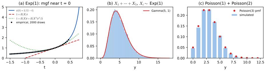
fig_3_s6. Supplementary figure for Wasserman (2004), Section 3.6. Download: PDF · SVG3.7 Appendix
p. 58 Expectation as an integral. The appendix sketches how \(\int r(x)\,\d F(x)\) is defined for a general (measurable) function \(r\) and a general distribution \(F\), discrete, continuous or neither, in three steps: simple functions, non-negative functions as limits of simple ones, and general functions as differences of non-negative ones.
Filling the gap 3.13: the three-step construction, with one correction p. 58
Step 1 (simple functions). If \(r\) takes the value \(a_i\) on the set \(A_i\), where \(A_1,\dots,A_k\) partition the real line, then
\[ \int r(x)\,\d F(x)=\sum_{i=1}^ka_i\,\P(X\in A_i). \]The book writes \(\P(r(X)\in A_i)\) here; since the \(A_i\) are sets of values of \(X\) on which \(r\) is constant, the probability that belongs in the formula is \(\P(X\in A_i)\) (equivalently \(\P(r(X)=a_i)\) when the \(a_i\) are distinct).
Step 2 (non-negative functions). For \(r\ge0\), \(\int r\,\d F=\lim_i\int r_i\,\d F\) for any sequence of simple functions \(0\le r_i\uparrow r\). Step 3. \(\int r\,\d F\)\({}=\int r^+\,\d F-\int r^-\,\d F\) with \(r^+=\max(r,0)\), \(r^-=\max(-r,0)\), when both are finite.
Why the definition makes sense, and why it agrees with sums and integrals
A sequence always exists. Take \(r_i(x)\)\({}=\min\{\lfloor2^ir(x)\rfloor/2^i,\;i\}\): it is simple (finitely many values), increasing in \(i\), and converges to \(r(x)\) at every \(x\), with \(0\le r-r_i\le2^{-i}\) wherever \(r\le i\).
The limit does not depend on the sequence. If \(r_i\uparrow r\) and \(s\le r\) is simple, then \(\lim_i\int r_i\,\d F\ge\int s\,\d F\) (for \(\varepsilon>0\) the sets \(\{r_i\ge(1-\varepsilon)s\}\) increase to the whole line, and continuity of probability on each of the finitely many sets where \(s\) is constant gives \(\lim_i\int r_i\,\d F\ge(1-\varepsilon)\int s\,\d F\)). Applying this with \(s\) running along a second sequence \(s_j\uparrow r\) gives \(\lim_i\int r_i\ge\lim_j\int s_j\), and by symmetry equality. This is the monotone convergence theorem in its simplest form.
Agreement with (3.1). For a discrete \(X\), choosing the \(A_i\) to contain one support point each shows \(\int r\,\d F=\sum_xr(x)f(x)\) for simple \(r\), and the limit passes through the sum. For a continuous \(X\), \(\P(X\in A_i)=\int_{A_i}f(x)\,\d x\), so \(\int r\,\d F=\int r(x)f(x)\,\d x\) for simple \(r\), and the monotone limit passes through the integral. The mixed case is the sum of the two. Linearity and the other properties used in this chapter all follow from the simple-function case by taking limits. ∎
Notes on the text
Slips found while writing these notes. The first two are in the author's errata lists on the book's website; the others are not, and the evidence is given.
p. 54, Definition 3.22: stray "dx" in the discrete case
The discrete-case sums in (3.13) and (3.14) carry a "\(\d x\)". Listed in the author's errata. Corrected in Definition 3.7.
p. 58, Example 3.35: "\(Y=Y_1+Y+2\)"
Should read \(Y=Y_1+Y_2\). Listed in the author's errata (second printing).
p. 48, Example 3.5: an \(\infty-\infty\) step
The integration by parts produces \([x\tan^{-1}x]_0^\infty-\int_0^\infty\tan^{-1}x\,\d x\), a difference of two infinite quantities, which has no value; the conclusion \(\E|X|=\infty\) is right but does not follow from that display. Evidence and a correct argument: \(\int_0^Mx/(1+x^2)\,\d x\)\({}=\tfrac12\log(1+M^2)\to\infty\) (Filling the gap 3.1, Figure 3.S1(c)).
p. 58, Appendix: \(\P(r(X)\in A_i)\) should be \(\P(X\in A_i)\)
The sets \(A_1,\dots,A_k\) partition the domain of \(r\) (values of \(X\)), not its range, so the weight of the value \(a_i\) is \(\P(X\in A_i)\). Evidence: with \(r=I_{[0,1]}\), \(A_1=[0,1]\), \(A_2\) its complement and \(X\sim\Unif(0,2)\), the book's formula gives \(1\cdot\P(I_{[0,1]}(X)\in[0,1])+0\)\({}=1\), while \(\E\,r(X)=\P(X\le1)=\tfrac12\). See Filling the gap 3.13.
p. 58, table of mgfs: "Normal\((\mu,\sigma)\)"
The row is labelled with the standard deviation, but the formula \(\exp(\mu t+\sigma^2t^2/2)\) is that of \(N(\mu,\sigma^2)\), the book's notation elsewhere. A notational inconsistency only.
Minor wording: Exercise 3.4 asks for the position "after \(n\) units", meaning after \(n\) jumps; Exercise 3.22 defines \(Y\) and \(Z\) through "\(x\)", meaning the random \(X\).
3.8 Exercises
All 24 exercises of Chapter 3 (Wasserman, 2004, pp. 58–61), restated in my own words, with complete solutions (hidden). The computer experiments (3.9, 3.11, 3.19) are solved with the chapter's code.
Exercise 3.1. You start a game with \(c\) dollars. At each play your fortune is doubled or halved, each with probability \(1/2\), independently of the past. What is your expected fortune after \(n\) plays?
Solution
The fortune after \(n\) plays is \(X_n=c\prod_{i=1}^nM_i\), with \(M_i\) independent, \(\P(M_i=2)\)\({}=\P(M_i=\tfrac12)\)\({}=\tfrac12\), so \(\E M_i\)\({}=\tfrac12\cdot2+\tfrac12\cdot\tfrac12\)\({}=\tfrac54\). By the product rule (Result 3.4), \(\E X_n=c(5/4)^n\), which grows exponentially. Yet the typical fortune does not grow: \(\log_2(X_n/c)=\sum_i\log_2M_i\) is a symmetric random walk with steps \(\pm1\), so the median of \(X_n\) is \(c\) (for even \(n\)) and \(\P(X_n\le c)\ge\tfrac12\) for every \(n\). The mean is driven by rare long runs of doublings: \(\P(X_n=2^nc)=2^{-n}\) contributes \(c\) to the mean on its own. Checked by exact enumeration of all \(2^n\) outcomes for \(n=10\): \(\E X_{10}=c(1.25)^{10}=9.313c\).
Exercise 3.2. Show that \(\V(X)=0\) if and only if \(\P(X=c)=1\) for some constant \(c\).
Solution
This is Result 3.6, proved there with Chebyshev's inequality and continuity of probability.
Exercise 3.3. Let \(X_1,\dots,X_n\sim\Unif(0,1)\) independently and \(Y_n=\max\{X_1,\dots,X_n\}\). Find \(\E(Y_n)\).
Solution
\(\P(Y_n\le y)\)\({}=\P(X_1\le y,\dots,X_n\le y)\)\({}=y^n\) for \(0\le y\le1\), by independence. So \(Y_n\) has density \(ny^{n-1}\) on \((0,1)\) and \(\E Y_n\)\({}=\int_0^1ny^n\,\d y\)\({}=\frac n{n+1}\). Alternatively, by the tail formula of Exercise 3.7, \(\E Y_n\)\({}=\int_0^1(1-y^n)\,\d y\)\({}=1-\frac1{n+1}\). The \(n\) points cut \([0,1]\) into \(n+1\) gaps of equal expected length \(1/(n+1)\); the last gap is \(1-Y_n\).
Exercise 3.4. A particle starts at 0 and moves in unit jumps: left with probability \(p\), right with probability \(1-p\), independently. Let \(X_n\) be its position after \(n\) jumps. Find \(\E(X_n)\) and \(\V(X_n)\) (a random walk).
Solution
\(X_n=\sum_{i=1}^nJ_i\) with independent \(J_i\in\{-1,+1\}\), \(\P(J_i=-1)=p\). Then \(\E J_i=(1-p)-p=1-2p\), \(\E J_i^2=1\), \(\V J_i=1-(1-2p)^2=4p(1-p)\). By linearity and (3.8): \(\E X_n=n(1-2p)\) and \(\V X_n=4np(1-p)\). The drift grows like \(n\) and the standard deviation like \(\sqrt n\), so for \(p\ne\tfrac12\) the drift eventually dominates.
Exercise 3.5. A fair coin is tossed until the first head. What is the expected number of tosses?
Solution
The number of tosses is Geometric\((\tfrac12)\), so the mean is \(1/p=2\) (Filling the gap 3.4). Directly by conditioning on the first toss: \(\E N\)\({}=\tfrac12\cdot1+\tfrac12(1+\E N)\), so \(\E N=2\).
Exercise 3.6. Prove Theorem 3.6 (the rule of the lazy statistician) for discrete random variables.
Solution
See the first part of the proof of Result 3.1: group the support points \(x_i\) of \(X\) according to the value \(y_j=r(x_i)\); then \(f_Y(y_j)\)\({}=\sum_{i:r(x_i)=y_j}f_X(x_i)\), and regrouping (allowed for non-negative series, and then for absolutely convergent ones) gives \(\sum_ir(x_i)f_X(x_i)\)\({}=\sum_jy_jf_Y(y_j)\).
Exercise 3.7. Let \(X\) be continuous with \(\P(X>0)=1\) and finite mean. Show that \(\E(X)\)\({}=\int_0^\infty\P(X>x)\,\d x\).
Solution
By Tonelli's theorem (works for every non-negative \(X\), continuous or not, and even when \(\E X=\infty\)): \(x=\int_0^\infty I(t<x)\,\d t\) for \(x\ge0\), so
\[ \begin{aligned}\E X&=\int_0^\infty\!\!\int_0^\infty I(t<x)\,\d t\,\d F(x)\\&=\int_0^\infty\!\!\int I(x>t)\,\d F(x)\,\d t\\&=\int_0^\infty\P(X>t)\,\d t,\end{aligned} \]the exchange being allowed because the integrand is non-negative.
By parts (the book's hint): for \(M>0\), with \(u=x\) and \(v=-(1-F(x))\),
\[ \begin{aligned}\int_0^Mxf(x)\,\d x&=\big[-x(1-F(x))\big]_0^M+\int_0^M(1-F(x))\,\d x\\&=-M\{1-F(M)\}+\int_0^M\P(X>x)\,\d x.\end{aligned} \]Since \(M\{1-F(M)\}\le\int_M^\infty xf(x)\,\d x\to0\) when \(\E X<\infty\) (the tail of a convergent integral), letting \(M\to\infty\) gives the result. Example: for Exp\((\beta)\), \(\int_0^\infty e^{-x/\beta}\,\d x\)\({}=\beta\).
Exercise 3.8. Prove Theorem 3.17.
Solution
See the proof of Result 3.7: \(\E\overline X_n=\mu\) and \(\V\overline X_n=\sigma^2/n\) by linearity and (3.8), and \(\E(S_n^2)=\sigma^2\) from the identity \(\SS\)\({}=\sum(X_i-\mu)^2-n(\overline X_n-\mu)^2\). Filling the gap 3.2 adds the variance of \(S_n^2\).
Exercise 3.9 (computer experiment). Let \(X_1,\dots,X_n\sim N(0,1)\) and plot \(\overline X_n\) against \(n=1,\dots,10{,}000\). Repeat with Cauchy draws, and explain the difference.
Solution
See Figure 3.S1 (
fig_3_s1, three runs of each). The normal running means settle at 0, with fluctuations of size \(\sd(\overline X_n)=1/\sqrt n\) (0.01 at \(n=10{,}000\)). The Cauchy running means keep jumping, even after thousands of draws. The reason is Filling the gap 3.1: the Cauchy has no mean, so there is nothing for \(\overline X_n\) to settle on; in fact \(\overline X_n\) has the same standard Cauchy distribution for every \(n\), so averaging gains nothing, and occasional enormous draws (\(\P(|X|>x)\approx2/(\pi x)\)) dominate the sum.Exercise 3.10. Let \(X\sim N(0,1)\) and \(Y=e^X\). Find \(\E(Y)\) and \(\V(Y)\).
Solution
These are values of the normal mgf \(\psi(t)=e^{t^2/2}\): \(\E Y=\psi(1)=e^{1/2}\approx1.6487\) and \(\E Y^2=\E e^{2X}=\psi(2)=e^2\), so \(\V Y=e^2-e=e(e-1)\approx4.6708\). (\(Y\) is lognormal; confirmed by numerical integration.)
Exercise 3.11 (computer experiment: a model of a stock price). Let \(Y_1,Y_2,\dots\) be independent with \(\P(Y_i=1)=\P(Y_i=-1)=\tfrac12\), and \(X_n=\sum_{i=1}^nY_i\). (a) Find \(\E(X_n)\) and \(\V(X_n)\). (b) Simulate and plot \(X_n\) for \(n\le10{,}000\), several times. Why do the runs look so different, and why does one "see" patterns?
Solution
(a) \(\E Y_i=0\), \(\V Y_i=1\), so \(\E X_n=0\) and \(\V X_n=n\) (Exercise 3.4 with \(p=\tfrac12\)). (b) Figure 3.S2 (
fig_3_s2) shows four runs. Although every run has mean 0, its standard deviation is \(\sqrt n\), 100 at \(n=10{,}000\): the runs fan out within the band \(\pm2\sqrt n\) and end far apart (here between about 17 and 165). Two runs differ by a variable with variance \(2n\). Long excursions to one side are typical, not exceptional (by the arcsine law, the fraction of time spent above 0 is more likely to be near 0 or 1 than near \(\tfrac12\)), which is why the paths seem to show trends that are pure chance.
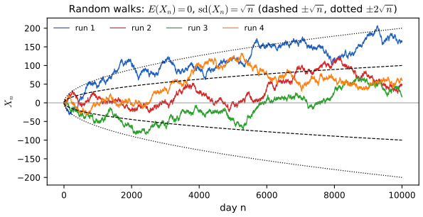
fig_3_s2. Supplementary figure for Wasserman (2004), Exercise 3.11. Download: PDF · SVGExercise 3.12. Prove the table of Section 3.4 for the Bernoulli, Poisson, uniform, exponential, gamma and beta distributions.
Solution
See Filling the gap 3.4 (Bernoulli, Poisson: the factorial moment \(\E\{X(X-1)\}=\lambda^2\)) and Filling the gap 3.5 (uniform, exponential, gamma: \(\E X^k\)\({}=\beta^k\Gamma(\alpha+k)/\Gamma(\alpha)\); beta: \(\E X^k\)\({}=B(\alpha+k,\beta)/B(\alpha,\beta)\)), which follow the book's hints of multiplying and dividing by the normalising constant of a neighbouring density.
Exercise 3.13. Flip a fair coin; on heads draw \(X\sim\Unif(0,1)\), on tails \(X\sim\Unif(3,4)\). (a) Find the mean of \(X\). (b) Find its standard deviation.
Solution
Let \(H\) indicate heads. (a) \(\E X\)\({}=\E\,\E(X\given H)\)\({}=\tfrac12\cdot\tfrac12+\tfrac12\cdot\tfrac72\)\({}=2\). (b) By the law of total variance, \(\V(X\given H)=\tfrac1{12}\) in both cases and \(\E(X\given H)\) takes the values \(\tfrac12\) and \(\tfrac72\) with probability \(\tfrac12\) each, so \(\V\,\E(X\given H)=\tfrac94\). Hence \(\V X\)\({}=\tfrac1{12}+\tfrac94\)\({}=\tfrac73\) and \(\sd(X)=\sqrt{7/3}\approx1.528\). Check: \(\E X^2\)\({}=\tfrac12\cdot\tfrac13+\tfrac12\cdot\tfrac{37}3\)\({}=\tfrac{19}3\) and \(\tfrac{19}3-4=\tfrac73\). Almost all of the variance is the gap between the two groups.
Exercise 3.14. Show that \(\Cov\big(\sum_{i=1}^ma_iX_i,\sum_{j=1}^nb_jY_j\big)\)\({}=\sum_{i=1}^m\sum_{j=1}^na_ib_j\Cov(X_i,Y_j)\).
Solution
See the proof of Result 3.9: centre each variable, multiply out the two finite sums, and apply linearity of expectation term by term.
Exercise 3.15. Let \(f_{X,Y}(x,y)=\tfrac13(x+y)\) for \(0\le x\le1\), \(0\le y\le2\), and 0 otherwise. Find \(\V(2X-3Y+8)\).
Solution
The density integrates to \(\tfrac13\int_0^1(2x+2)\,\d x=1\). Marginals: \(f_X(x)=\tfrac23(x+1)\) on \([0,1]\), \(f_Y(y)=\tfrac13(y+\tfrac12)\) on \([0,2]\). Then
\[ \begin{aligned}&\E X=\tfrac59,\quad \E X^2=\tfrac7{18},\quad \V X=\tfrac{13}{162};\\ &\E Y=\tfrac{11}9,\quad \E Y^2=\tfrac{16}9,\quad \V Y=\tfrac{23}{81};\\ &\E XY=\tfrac23,\quad \Cov(X,Y)=\tfrac23-\tfrac{55}{81}=-\tfrac1{81}.\end{aligned} \]The constant 8 does not affect the variance, and by Result 3.9
\[ \begin{aligned}\V(2X-3Y+8)&=4\V X+9\V Y-12\Cov(X,Y)\\&=\tfrac{26}{81}+\tfrac{207}{81}+\tfrac{12}{81}\\&=\tfrac{245}{81}\approx3.0247,\end{aligned} \]confirmed by numerical double integration.
Exercise 3.16. Show that \(\E\{r(X)s(Y)\given X\}\)\({}=r(X)\E\{s(Y)\given X\}\), and that \(\E\{r(X)\given X\}=r(X)\).
Solution
Part 2 of Filling the gap 3.8: given \(X=x\), \(r(X)=r(x)\) is a constant and comes out of the conditional sum or integral; take \(s\equiv1\) for the second statement.
Exercise 3.17. Prove the law of total variance, \(\V(Y)\)\({}=\E\,\V(Y\given X)+\V\,\E(Y\given X)\).
Solution
See the proof of Result 3.12, which follows the book's hint: expand \(\{(Y-b(X))+(b(X)-m)\}^2\) and take each expectation by conditioning on \(X\); the cross term vanishes.
Exercise 3.18. Show that if \(\E(X\given Y=y)=c\) for some constant \(c\), then \(X\) and \(Y\) are uncorrelated.
Solution
\(\E X=\E\,\E(X\given Y)=c\) and \(\E(XY)\)\({}=\E\{Y\,\E(X\given Y)\}\)\({}=c\,\E Y\), so \(\Cov(X,Y)=c\E Y-c\E Y=0\) (part 6 of Filling the gap 3.8). The converse is false: in Filling the gap 3.3, \(\Cov(X,X^2)=0\) but \(\E(X^2\given X)=X^2\) is not constant.
Exercise 3.19 (computer experiment: a sampling distribution). Let \(X_1,\dots,X_n\sim\Unif(0,1)\). Plot the density \(f_X\). Find \(\E(\overline X_n)\) and \(\V(\overline X_n)\) and plot them against \(n\). Simulate the distribution of \(\overline X_n\) for \(n=1,5,25,100\), check the simulated mean and variance against the theory, and describe how the sampling distribution changes with \(n\).
Solution
By Result 3.7, \(\E\overline X_n=\tfrac12\) and \(\V\overline X_n=\frac1{12n}\). Figure 3.S3 (
fig_3_s3, 10,000 samples of each size) gives simulated means 0.5031, 0.5014, 0.5002, 0.4997 and variances 0.08395, 0.01638, 0.00334, 0.00085, against \(\tfrac1{12n}\)\({}=0.08333,0.01667,0.00333,0.00083\). The distribution of the data is flat and stays flat; the distribution of the statistic \(\overline X_n\) concentrates around \(\tfrac12\) at the rate \(1/\sqrt n\) and becomes bell-shaped (already close to the normal curve at \(n=5\)): the law of large numbers and the central limit theorem of Chapter 5, seen in advance.
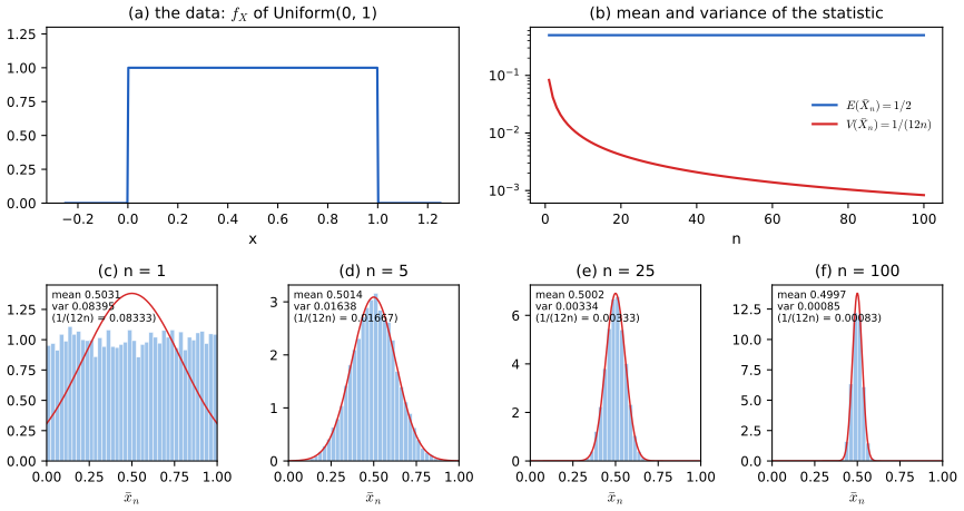
fig_3_s3. Supplementary figure for Wasserman (2004), Exercise 3.19. Download: PDF · SVGExercise 3.20. Prove Lemma 3.21.
Solution
See the proof of Result 3.10: \(\E(\bA\bX)=\bA\bmu\) row by row, and \(\V(\bA\bX)\)\({}=\E\{\bA(\bX-\bmu)(\bX-\bmu)^\T\bA^\T\}\)\({}=\bA\bSigma\bA^\T\); the vector case is \(\bA=\ba^\T\).
Exercise 3.21. Suppose \(\E(Y\given X)=X\). Show that \(\Cov(X,Y)=\V(X)\).
Solution
By iterated expectations and "taking out what is known", \(\E(XY)\)\({}=\E\{X\,\E(Y\given X)\}\)\({}=\E(X^2)\) and \(\E Y=\E\,\E(Y\given X)=\E X\). So \(\Cov(X,Y)=\E X^2-(\E X)^2=\V X\). Example: \(Y=X+\varepsilon\) with \(\E(\varepsilon\given X)=0\), a regression with slope 1.
Exercise 3.22. Let \(X\sim\Unif(0,1)\), \(0<a<b<1\), \(Y=I(0<X<b)\) and \(Z=I(a<X<1)\). (a) Are \(Y\) and \(Z\) independent? (b) Find \(\E(Y\given Z)\).
Solution
(a) No. \(\P(Y=1,Z=1)=\P(a<X<b)=b-a\), while \(\P(Y=1)\P(Z=1)=b(1-a)=b-ab\). These are equal only if \(a=ab\), i.e. \(b=1\), which is excluded. (Also: \(Z=0\) forces \(X\le a<b\), so \(Y=1\); learning \(Z\) changes the odds of \(Y\).)
(b) \(Z\) takes two values. \(\E(Y\given Z=1)\)\({}=\P(X<b\given X>a)\)\({}=\frac{b-a}{1-a}\) and \(\E(Y\given Z=0)\)\({}=\P(X<b\given X\le a)\)\({}=1\). So
\[ \E(Y\given Z)=1-Z\,\frac{1-b}{1-a}. \]Check by iterated expectations: \(\E\,\E(Y\given Z)\)\({}=1-(1-a)\frac{1-b}{1-a}\)\({}=b\)\({}=\P(X<b)\)\({}=\E Y\).
Exercise 3.23. Find the moment generating functions of the Poisson, normal and gamma distributions.
Solution
See Filling the gap 3.11: \(e^{\lambda(e^t-1)}\) for all \(t\); \(\exp(\mu t+\sigma^2t^2/2)\) for all \(t\) (complete the square); \((1-\beta t)^{-\alpha}\) for \(t<1/\beta\) (recognise a gamma density with scale \(\beta/(1-\beta t)\)).
Exercise 3.24. Let \(X_1,\dots,X_n\sim\mathrm{Exp}(\beta)\) independently. Find the mgf of \(X_i\), and prove that \(\sum_{i=1}^nX_i\sim\mathrm{Gamma}(n,\beta)\).
Solution
\(\psi_{X_i}(t)\)\({}=\int_0^\infty e^{tx}\beta^{-1}e^{-x/\beta}\,\d x\)\({}=(1-\beta t)^{-1}\) for \(t<1/\beta\). By Result 3.13(2), the sum has mgf \((1-\beta t)^{-n}\) on the same interval, which is the Gamma\((n,\beta)\) mgf of Filling the gap 3.11. Both are finite on the open interval \((-\infty,1/\beta)\ni0\), so by uniqueness (Result 3.14) the sum is Gamma\((n,\beta)\). Figure 3.S6(b) shows \(n=5\), \(\beta=1\).
▶ DemoExponential sums are gammaThe histogram of five-term sums follows the Gamma(5, 1) density; the mgf exists only for t < 1.
Demonstrations for this chapter
Each demonstration runs in the browser and links back to these notes. The ▶ Demo boxes above open them already set to the case under discussion.
| Demonstration | What you can see | Sections and results |
|---|---|---|
| The sample variance: n or n − 1 | Repeated samples from normal, uniform, exponential or Bernoulli populations, or from the book's nerve-pulse data: histograms of \(S_n^2\), running averages of \(\SS/(n-1)\), \(\SS/n\) and \(\SS/(n+1)\), and the mean squared error of \(\SS/d\) against \(d\) with the best divisor. Presets: 1 normal, \(n=5\); 2 \(n=2\); 3 exponential data; 4 nerve data; 5 coin flips. | 3.3; Result 3.7, Filling the gap 3.2 |
| Conditional expectation and the law of total variance | Three two-stage experiments (a binomial count with a beta proportion, the broken stick, a coin then a uniform): the conditional mean as a function, binned simulated means, the exact marginal of the second stage, and the two terms \(\E\,\V(Y\given X)\) and \(\V\,\E(Y\given X)\) against simulation. Presets: 1 Example 3.28; 2 \(n=50\); 3 Beta(30, 30); 4 Examples 3.23 and 3.25; 5 Exercise 3.13. | 3.5; Results 3.11, 3.12, Filling the gap 3.9 |
| Moment generating functions and sums | Sums of independent Bernoulli, Poisson, exponential, uniform or normal variables: the exact and empirical log mgf with its tangent and quadratic at 0, the moments from the derivatives of \(\psi\), and the histogram of the sums against the law the mgf identifies; a standardised view whose log mgf approaches \(t^2/2\). Presets: 1 binomial; 2 Poisson; 3 gamma; 4 Irwin–Hall; 5 standardised. | 3.6; Results 3.13, 3.14, Filling the gaps 3.10–3.12 |
Related demonstrations in the companion courses: the Gaussian maximum likelihood demo (Foundations of Deep Learning), the gamma-Poisson demo and the Poisson limit demo (Statistical Methods for Modern Biology), and the first-year estimators and central limit theorem demos. The Python code that produces every figure of this page is code/ch03_expectation.py (see the code index).
References
- Wasserman, L. (2004). All of Statistics: A Concise Course in Statistical Inference. Springer, New York. Chapter 3, pp. 47–61. www.stat.cmu.edu/~larry/all-of-statistics.
- Billingsley, P. (1995). Probability and Measure, 3rd edition. Wiley, New York.
- Casella, G. and Berger, R. L. (2002). Statistical Inference, 2nd edition. Duxbury, Pacific Grove.
- Curtiss, J. H. (1942). A note on the theory of moment generating functions. The Annals of Mathematical Statistics, 13(4), 430–433.
- Feller, W. (1968). An Introduction to Probability Theory and Its Applications, Volume 1, 3rd edition. Wiley, New York.
- Grimmett, G. and Stirzaker, D. (2001). Probability and Random Processes, 3rd edition. Oxford University Press, Oxford.
- Hall, P. (1927). The distribution of means for samples of size N drawn from a population in which the variate takes values between 0 and 1, all such values being equally probable. Biometrika, 19(3/4), 240–245.
- Heyde, C. C. (1963). On a property of the lognormal distribution. Journal of the Royal Statistical Society, Series B, 25(2), 392–393.
- Irwin, J. O. (1927). On the frequency distribution of the means of samples from a population having any law of frequency with finite moments, with special reference to Pearson's Type II. Biometrika, 19(3/4), 225–239.
- Knuth, D. E. (1997). The Art of Computer Programming, Volume 2: Seminumerical Algorithms, 3rd edition. Addison-Wesley, Reading.
- Marsaglia, G. and Tsang, W. W. (2000). A simple method for generating gamma variables. ACM Transactions on Mathematical Software, 26(3), 363–372.
The numerical statements in the text (the examples of Sections 3.1–3.6, the table of means and variances, the variance of \(S_n^2\) and the best divisor, the multinomial and multivariate normal moments, the two-stage examples and the law of total variance, the table of moment generating functions and the identified laws of sums, and the answers to the exercises) were confirmed numerically.