Statistical Decision Theory
How should we choose between estimators? Decision theory answers by attaching a loss to every error and comparing estimators through their average loss, the risk, as a function of the unknown parameter. Risk functions usually cross, so the theory needs a one-number summary: the worst case (leading to minimax rules) or an average over a prior (leading to Bayes rules). This short chapter of the book states the main facts, often without proof. These notes prove them all: the posterior mean, median and mode as Bayes rules, least favourable priors and the restricted Normal mean, the local minimax property of maximum likelihood (with superefficiency and the van Trees inequality), the minimax risk for many Normal means (where the book's formula needs correcting), the admissibility of the sample mean, and Stein's paradox, with the reason why three dimensions is the threshold.
Ch. 1 Probability Ch. 2 Random variables Ch. 3 Expectation Ch. 4 Inequalities Ch. 5 Convergence Ch. 6 Models and inference Ch. 7 Estimating the CDF Ch. 8 Bootstrap Ch. 9 Parametric inference Ch. 10 Hypothesis testing Ch. 11 Bayesian inference Ch. 12 Decision theory Ch. 13 Regression Ch. 14 Multivariate models Ch. 15 Independence Ch. 16 Causal inference Ch. 17 Directed graphs Ch. 18 Undirected graphs Ch. 19 Log-linear models Ch. 20 Curve estimation Ch. 21 Orthogonal functions Ch. 22 Classification Ch. 23 Stochastic processes Ch. 24 Simulation
How to read these notes
They follow the book. Sections carry the book's numbers (12.1 to 12.9) and every displayed equation that appears in the book carries the book's own equation number, e.g. \((12.12)\). Numbered items keep the book's numbers (Definition 12.1, Theorem 12.10, Example 12.15); results the book states without a number, and the new results needed to fill its gaps, are lettered (Definition 12.A, Theorem 12.B, ...). Equations without a number are steps that the book skips.
Filling the gaps. Wherever the book says "it can be shown", quotes a result without proof, or leaves an argument implicit, an orange Filling the gap box gives the full argument. Proofs and derivations start hidden: open one with its bar, or use the button below.
Figures and demonstrations. The three figures of the chapter are reproduced (Figures 12.1 to 12.3), and six supplementary figures (12.S1 to 12.S6) illustrate gaps filled in the notes; all are computed by the Python code. The ▶ Demo boxes open an interactive demonstration already set to the case being discussed.
Main reference
L. Wasserman, All of Statistics: A Concise Course in Statistical Inference, Springer (2004), Chapter 12, pages 193–205 (book website: www.stat.cmu.edu/~larry/all-of-statistics). Section, equation, example and exercise numbers below refer to this book. Further reading is listed in the references.
The explanations, derivations, figures and code are my own; equations are cited by their numbers in the book.
Companion courses
Decision theory also appears, from the prediction side, in three companion courses on this site. The overlapping material is:
- Bayesian and Probabilistic Machine Learning, Section 1.5 (decision theory): minimum expected loss for classification (Result 1.16), the conditional mean as the squared-loss optimum (Result 1.18) and the Minkowski loss with its mean, median and mode (Result 1.19); and in Chapter 2 the Beta posterior of a proportion (Result 2.3) and the Normal posterior of a mean (Result 2.16). Its decision theory demo shows loss matrices and the reject option.
- Foundations of Deep Learning, Section 4.2 (decision theory for regression: Result 4.9, the Minkowski loss in Result 4.10 and why its limit is not the mode, Result 4.11) with the Minkowski loss demo, and Section 5.2 (decision theory for classification, Results 5.5 and 5.6).
- Statistical Learning: Theory and Methods, Result 3.20: Stein's lemma, used there for the degrees of freedom of a fit and here for the risk of the James-Stein estimator; its shrinkage paths demo shows ridge and lasso shrinkage.
- Statistical Methods for Modern Biology, Filling the gap 2.17: the posterior mean of a proportion as a compromise between the prior mean and the data.
Those courses use decision theory to choose a prediction once the predictive distribution is known; this chapter uses it to compare estimators over all values of the parameter, which is what makes the minimax and admissibility questions appear. Where a proof there is identical, these notes give the statement and a short argument and link to it. New here: Bayes estimators made rigorous, including why a literal zero-one loss fails for a continuous parameter (Filling the gap 12.5), least favourable priors and limits of Bayes rules (12.7), the restricted Normal mean (12.10), superefficiency and the van Trees inequality (12.11), Pinsker's minimax risk (12.13), the admissibility of the sample mean (12.15), and Stein's paradox with the reason it starts in dimension three (12.17, 12.18).
The chapter at a glance
- 12.1 A loss \(L(\th,\ht)\) scores an estimate; the risk \(R(\th,\ht)\) is its expectation (Definition 12.1); under squared loss the risk is the mean squared error.
- 12.2 Risk functions cross (Examples 12.2 and 12.3), so they are summarised by their maximum or by their average under a prior (Definition 12.4), and the two summaries can disagree (Filling the gap 12.3).
- 12.3 A Bayes rule minimises the posterior risk at each data set (Theorem 12.7): posterior mean, median or mode for squared, absolute or zero-one loss (Theorem 12.8).
- 12.4 A Bayes rule whose risk never exceeds its Bayes risk is minimax (Theorems 12.10 and 12.11); limits of Bayes risks give the same conclusion (Theorem 12.A); the Normal mean (Theorem 12.14) and a restricted Normal mean (Example 12.15).
- 12.5 In regular parametric models the MLE is locally asymptotically minimax (12.11) and close to Bayes (12.12), but not with many parameters (Example 12.16, 12.13).
- 12.6 Admissibility (Definition 12.17): Bayes rules are admissible (Theorem 12.19), so is the sample mean (Theorem 12.20); links with minimaxity (Theorems 12.21 to 12.23).
- 12.7 For three or more Normal means the James-Stein estimator dominates the observations (Theorem 12.D), and dimension three is exactly where Blyth's admissibility argument fails (12.18).
Notation. The parameter \(\th\) lives in \(\Theta\); data \(X\) (or \(X_1,\dots,X_n\)) have density \(f(x;\th)\), also written \(f(x\given\th)\) when \(\th\) is given a prior density \(f(\th)\). An estimator, or decision rule, is a function \(\ht=\ht(X)\) of the data; \(\P_\th\), \(\E_\th\), \(\V_\th\) are computed under \(f(\cdot;\th)\). \(\bX\) is the sample mean, \(\phi\) and \(\Phi\) the standard Normal density and cdf, \(\ind\{\cdot\}\) an indicator and \(z_+=\max\{z,0\}\). Unless stated otherwise the loss is squared error.
Prerequisites. Expectation, conditional expectation and the rule of iterated expectations (Chapter 3), the Cauchy-Schwarz and Chebyshev inequalities and the Kullback-Leibler divergence (Chapter 4), the bias-variance decomposition (Theorem 6.9), Fisher information and the MLE (Chapter 9 of the book) and Bayes' theorem for parameters (Chapter 11 of the book). See the course home.
12.1 Preliminaries
p. 193 We have met several ways of producing estimators: maximum likelihood, the method of moments, the posterior mean, and many more are possible. Decision theory is the formal framework for comparing them. In its language an estimator \(\ht\) of \(\th\in\Theta\) is a decision rule and its possible values are actions. The quality of an action is measured by a loss.
Definition 12.A (loss function) p. 193
A loss function is a map \(L:\Theta\times\Theta\to[0,\infty)\); \(L(\th,\ht)\) is the price of reporting \(\ht\) when the truth is \(\th\). Standard choices are
\[ \begin{aligned} &(\th-\ht)^2 &&\text{squared error loss}, \\ &|\th-\ht| &&\text{absolute error loss}, \\ &|\th-\ht|^p &&L_p\text{ loss}, \\ &\ind\{\ht\ne\th\} &&\text{zero-one loss}, \\ &\int\log\Big(\frac{f(x;\th)}{f(x;\ht)}\Big)f(x;\th)\,\d x &&\text{Kullback-Leibler loss}. \end{aligned} \]p. 194 An estimator is a function of the data, \(\ht=\ht(X)\), so its loss is random. To assess the estimator we average the loss over the data.
Definition 12.1 (risk) p. 194
The risk of an estimator \(\ht\) is the function of \(\th\)
\[ R(\th,\ht)=\E_\th\big(L(\th,\ht)\big)=\int L\big(\th,\ht(x)\big)f(x;\th)\,\d x . \]Under squared error loss the risk is the mean squared error, \(R(\th,\ht)=\E_\th(\ht-\th)^2\)
See also (companion course): the first-year notes prove the same decomposition as Theorem 1.1.
Filling the gap 12.1: three remarks on losses and risks pp. 193–194
(a) The risk always exists, but may be infinite. Because \(L\ge0\), the integral defining \(R(\th,\ht)\) is well defined in \([0,\infty]\). For \(X\sim\N(\th,1)\) the estimator \(\ht=1/X\) has infinite risk at every \(\th\) under squared loss.
(b) Kullback-Leibler loss. It is nonnegative, and zero exactly when the two densities agree (Gibbs' inequality, Result 4.10). In the Normal location model \(\N(\th,\sigma^2)\) it equals \((\th-\ht)^2/(2\sigma^2)\), half the squared error in units of \(\sigma^2\). In a smooth one-parameter model it is locally quadratic, \(\KL(\th,\th+h)=\tfrac12I(\th)h^2+o(h^2)\) with \(I\) the Fisher information, which is one reason why squared error is the default loss. But it can be infinite: for Bernoulli data the MLE \(\bX\) equals 0 with probability \((1-p)^n>0\), and then the loss \(p\log(p/0)\) is infinite, so the MLE has infinite Kullback-Leibler risk for every \(n\) and every \(0<p<1\).
(c) Risk is a function, not a number. \(R(\cdot,\ht)\) depends on the unknown \(\th\); the whole chapter is about how to compare such functions.
Derivations
(a) \(\E_\th(1/X-\th)^2\)
(b) For the Normal model, \(\log f(x;\th)-\log f(x;\ht)\)
12.2 Comparing Risk Functions
p. 194 To compare two estimators we compare their risk functions. The first two examples show that this rarely gives a clear answer.
Example 12.2. p. 194 Let \(X\sim\N(\th,1)\), squared loss, \(\ht_1=X\) and \(\ht_2=3\) (an estimator that ignores the data). Then \(R(\th,\ht_1)=\E_\th(X-\th)^2=1\) and \(R(\th,\ht_2)=(3-\th)^2\). The constant guess is better exactly when \(|\th-3|<1\), i.e. \(2<\th<4\), and worse elsewhere: neither estimator dominates the other (Figure 12.1).
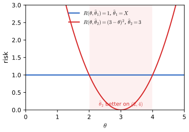
fig_12_1. Download: PDF · SVGExample 12.3. pp. 194–195 Let \(X_1,\dots,X_n\sim\Bern(p)\), \(Y=\sum_iX_i\) and squared loss. The MLE \(\widehat p_1=\bX\) is unbiased, so
\[ R(p,\widehat p_1)=\V(\bX)=\frac{p(1-p)}{n}. \]The posterior mean under a \(\Bet(\alpha,\beta)\) prior is \(\widehat p_2=(Y+\alpha)/(\alpha+\beta+n)\), with risk
\[ R(p,\widehat p_2)=\V_p(\widehat p_2)+\bias_p^2(\widehat p_2)=\frac{np(1-p)}{(\alpha+\beta+n)^2}+\Big(\frac{np+\alpha}{\alpha+\beta+n}-p\Big)^2. \]The choice \(\alpha=\beta=\sqrt{n/4}\) (explained in Example 12.12) gives \(\widehat p_2=(Y+\sqrt{n/4})/(n+\sqrt n)\), whose risk does not depend on \(p\) at all:
\[ R(p,\widehat p_2)=\frac{n}{4(n+\sqrt n)^2}. \]Figure 12.2 shows that again neither estimator dominates.
Filling the gap 12.2: the risk of the posterior mean, and the only constant-risk choice p. 195
With \(s=\alpha+\beta\), the risk of \(\widehat p_2=(Y+\alpha)/(n+s)\) is
\[ R(p,\widehat p_2)=\frac{np(1-p)+(\alpha-sp)^2}{(n+s)^2}=\frac{(s^2-n)p^2+(n-2\alpha s)p+\alpha^2}{(n+s)^2}, \]a quadratic in \(p\). It is constant if and only if both coefficients vanish, \(s^2=n\) and \(n=2\alpha s\), that is \(\alpha=\beta=\sqrt n/2\). So among all Beta-prior posterior means exactly one has constant risk, and its risk is \(\alpha^2/(n+s)^2=n/\{4(n+\sqrt n)^2\}\)
Derivation
\(Y\sim\Bin(n,p)\) has \(\E Y=np\) and \(\V Y=np(1-p)\). Hence \(\V(\widehat p_2)=np(1-p)/(n+s)^2\) and \(\bias=(np+\alpha)/(n+s)-p\)
The same calculation, for symmetric pseudo-counts only, is in Filling the gap 6.4(b) of Chapter 6.
Definition 12.4 (maximum risk and Bayes risk) p. 195
The maximum risk of \(\ht\) and its Bayes risk with respect to a prior density \(f(\th)\) are
\[ \bR(\ht)=\sup_\th R(\th,\ht), \tag{12.1} \] \[ r(f,\ht)=\int R(\th,\ht)f(\th)\,\d\th. \tag{12.2} \]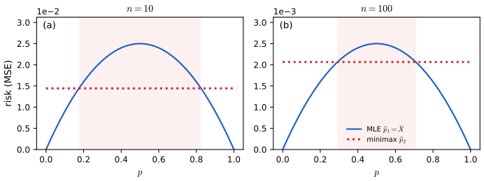
fig_12_2. Download: PDF · SVGExample 12.5. p. 196 For the two estimators of Example 12.3,
\[ \bR(\widehat p_1)=\max_{0\le p\le1}\frac{p(1-p)}{n}=\frac1{4n},\qquad \bR(\widehat p_2)=\frac{n}{4(n+\sqrt n)^2}, \]so \(\widehat p_2\) is better by maximum risk. Yet when \(n\) is large \(\widehat p_1\) has the smaller risk except in a small region around \(p=1/2\), which is why many statisticians prefer it: one-number summaries lose information. With the uniform prior \(f(p)=1\) the Bayes risks are
\[ r(f,\widehat p_1)=\int_0^1\frac{p(1-p)}{n}\,\d p=\frac1{6n},\qquad r(f,\widehat p_2)=\frac{n}{4(n+\sqrt n)^2}, \]and for \(n\ge20\) the MLE has the smaller Bayes risk. The answer depends on the prior; maximum risk needs no prior, which is its main appeal.
Filling the gap 12.3: where the two summaries disagree p. 196
- The crossing. \(r(f,\widehat p_2)>r(f,\widehat p_1)\) if and only if \(n>(2+\sqrt6)^2=10+4\sqrt6\approx19.80\), so "\(n\ge20\)" is exact for integer \(n\).
- Maximum risk always prefers \(\widehat p_2\), by a vanishing margin: \(\bR(\widehat p_2)/\bR(\widehat p_1)\)
\({}=\{\sqrt n/(\sqrt n+1)\}^2\approx1-2/\sqrt n\). - Bayes risk eventually prefers \(\widehat p_1\) by a fixed margin: \(r(f,\widehat p_2)/r(f,\widehat p_1)\)
\({}=3n/\{2(\sqrt n+1)^2\}\to3/2\). - The region where \(\widehat p_2\) wins is \(|p-\tfrac12|<\sqrt{2\sqrt n+1}/\{2(\sqrt n+1)\}\), of width about \(\sqrt2\,n^{-1/4}\): 0.288 either side of 1/2 for \(n=20\), 0.208 for \(n=100\), 0.152 for \(n=400\).
Derivations
\(\int_0^1p(1-p)\,\d p=\tfrac12-\tfrac13\)
(1) \(\frac1{6n}<\frac1{4(\sqrt n+1)^2}\iff2(\sqrt n+1)^2\)
(2) and (3) are divisions of the closed forms.
(4) \(\widehat p_2\) wins iff \(\frac{p(1-p)}n>\frac1{4(\sqrt n+1)^2}\)
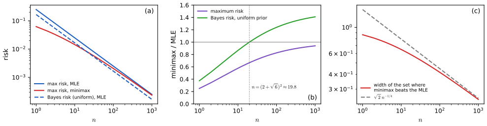
fig_12_s1. Download: PDF · SVGSee also: the Chapter 6 shrinkage demo shows the same constant-risk estimator as a bias-variance trade-off.
pp. 196–197 The two summaries lead to two ways of constructing estimators: minimise the maximum risk (minimax rules) or minimise the Bayes risk (Bayes rules).
Definition 12.6 (Bayes rule, minimax rule) p. 197
\(\ht\) is a Bayes rule with respect to the prior \(f\) if
\[ r(f,\ht)=\inf_{\tth}r(f,\tth), \tag{12.3} \]and \(\ht\) is a minimax rule if
\[ \sup_\th R(\th,\ht)=\inf_{\tth}\sup_\th R(\th,\tth), \tag{12.4} \]where in both cases the infimum is over all estimators \(\tth\).
12.3 Bayes Estimators
p. 197 Let \(f(\th)\) be a prior. By Bayes' theorem the posterior density is
\[ f(\th\given x)=\frac{f(x\given\th)f(\th)}{m(x)}=\frac{f(x\given\th)f(\th)}{\int f(x\given\th)f(\th)\,\d\th}, \tag{12.5} \]where \(m(x)=\int f(x,\th)\,\d\th\)
Theorem 12.7 (Bayes rules minimise the posterior risk) p. 197
The Bayes risk is the average posterior risk, \(r(f,\ht)=\int r(\ht\given x)\,m(x)\,\d x\). Consequently, if \(\ht(x)\) is, for each \(x\), the action that minimises the posterior risk \(r(\cdot\given x)\), then \(\ht\) is a Bayes rule.
Proof
Write the risk as an integral over the data, then use \(f(x\given\th)f(\th)=f(x,\th)\)
If \(\ht(x)\) minimises the integrand \(r(\cdot\given x)\) at every \(x\), then for any other rule \(\tth\), \(r(\tth\given x)\ge r(\ht\given x)\) for all \(x\), and integrating against \(m\) gives \(r(f,\tth)\ge r(f,\ht)\). ∎
Filling the gap 12.4: Theorem 12.7 with the fine print p. 197
- Swapping the integrals needs no integrability assumption: the integrand \(L(\th,\ht(x))f(x\given\th)f(\th)\) is nonnegative, so Tonelli's theorem applies (both sides may be \(+\infty\)).
- Data with \(m(x)=0\) do not matter: they form a set of marginal probability zero, so a Bayes rule may be defined arbitrarily there.
- Measurability. The pointwise minimiser must be a measurable function of \(x\) to be an estimator. In the cases below it is explicit (a posterior mean, a posterior quantile, a posterior mode); in general one needs a measurable selection theorem, available for instance when \(L\) is continuous and the actions range over a compact set.
- The converse holds almost everywhere. If some rule \(\ht^*\) minimises the posterior risk pointwise and \(r(f,\ht^*)<\infty\), then every Bayes rule \(\ht\) satisfies \(r(\ht\given x)=r(\ht^*\given x)\) for \(m\)-almost every \(x\). In particular, when the posterior risk has a unique minimiser (for squared loss, whenever the posterior variance is finite), the Bayes rule is unique up to sets of marginal probability zero. This uniqueness is what makes minimax rules unique in Examples 12.12 and 12.15 (Filling the gap 12.7(b)).
Proof of item 4
The function \(d(x)=r(\ht\given x)-r(\ht^*\given x)\) is nonnegative (\(\ht^*\) minimises pointwise), and \(\int d\,m\,\d x=r(f,\ht)-r(f,\ht^*)\)
Theorem 12.8 (posterior mean, median and mode) p. 198
Under squared error loss the Bayes estimator is the posterior mean,
\[ \ht(x)=\int\th\,f(\th\given x)\,\d\th=\E(\th\given X=x). \tag{12.7} \]Under absolute error loss it is a median of the posterior \(f(\th\given x)\); under zero-one loss it is the mode of the posterior.
Proof (squared loss, by the derivative)
The posterior risk \(\int(\th-a)^2f(\th\given x)\,\d\th\) is a function of the action \(a=\ht(x)\). Its derivative in \(a\) is \(-2\int(\th-a)f(\th\given x)\,\d\th\), which vanishes at \(a=\int\th f(\th\given x)\,\d\th\); by Theorem 12.7 this is the Bayes rule. The next box replaces this argument by one that needs no differentiation and also covers the other two losses. ∎
Filling the gap 12.5: mean, median and mode, proved p. 198
Fix the data \(x\); write \(F\) for the posterior cdf of \(\th\) and \(\mu=\E(\th\given x)\).
(a) Squared loss. If \(\E(\th^2\given x)<\infty\), then for every action \(a\)
\[ \E\big[(\th-a)^2\given x\big]=\V(\th\given x)+(\mu-a)^2 , \]so the posterior mean is the unique minimiser and the minimal posterior risk is the posterior variance.
(b) Absolute loss. If \(\E(|\th|\given x)<\infty\), then for \(a<b\)
\[ \E\big[|\th-b|\given x\big]-\E\big[|\th-a|\given x\big]=\int_a^b\big(2F(t)-1\big)\,\d t , \]and the set of minimisers is exactly the set of posterior medians (the \(t\) with \(F(t)\ge\tfrac12\) and \(F(t-)\le\tfrac12\)), a point or a closed interval.
(c) Zero-one loss, discrete parameter. If \(\Theta\) is countable, the posterior risk of \(a\) is \(\P(\th\ne a\given x)=1-f(a\given x)\), minimised by the posterior mode(s) (Exercise 12.3).
(d) Zero-one loss, continuous parameter. If the posterior has a density, \(\P(\th=a\given x)=0\) for every \(a\), so every estimator has posterior risk 1: the literal zero-one loss cannot single out the mode. The statement must be read through the window loss \(L_\epsilon(\th,a)=\ind\{|\th-a|>\epsilon\}\), whose Bayes action \(a_\epsilon\) is the centre of the interval of length \(2\epsilon\) with the largest posterior probability. If the posterior density \(g\) is continuous, has a unique maximiser \(\th^*\) and satisfies \(\sup_{|t-\th^*|\ge\delta}g(t)<g(\th^*)\) for every \(\delta>0\), then \(a_\epsilon\to\th^*\) as \(\epsilon\to0\): the mode is the limit of Bayes rules.
Proofs
(a) Write \(\th-a=(\th-\mu)+(\mu-a)\) and expand: \(\E[(\th-a)^2\given x]=\E[(\th-\mu)^2\given x]\)
(b) For real \(\th\) and \(a<b\), \(|\th-b|-|\th-a|=\int_a^b\big(\ind\{\th\)
(c) For \(a\in\Theta\), \(\E[\ind\{\th\ne a\}\given x]=1-f(a\given x)\); for \(a\notin\Theta\) it is 1. The smallest value comes from the largest posterior probability.
(d) The posterior risk of \(a\) under \(L_\epsilon\) is \(1-\int_{a-\epsilon}^{a+\epsilon}g\), so \(a_\epsilon\) maximises \(G_\epsilon(a)=\int_{a-\epsilon}^{a+\epsilon}g\). Suppose \(a_\epsilon\not\to\th^*\): then there are \(\delta>0\) and \(\epsilon_k\to0\) with \(|a_{\epsilon_k}-\th^*|\ge\delta\). For \(\epsilon_k<\delta/2\) every point of the window around \(a_{\epsilon_k}\) is at distance at least \(\delta/2\) from \(\th^*\), so \(G_{\epsilon_k}(a_{\epsilon_k})\le2\epsilon_k(g(\th^*)-\eta)\) with \(\eta=g(\th^*)-\sup_{|t-\th^*|\ge\delta/2}g(t)\)
Example. One success in ten trials with a uniform prior gives the posterior \(\Bet(2,10)\), skewed to the right: mode 0.1, median 0.1480, mean 0.1667. With \(\epsilon=0.05\) the window action is 0.1074, and it tends to 0.1 as \(\epsilon\to0\) (Figure 12.S2). For a symmetric unimodal posterior the three estimators coincide.
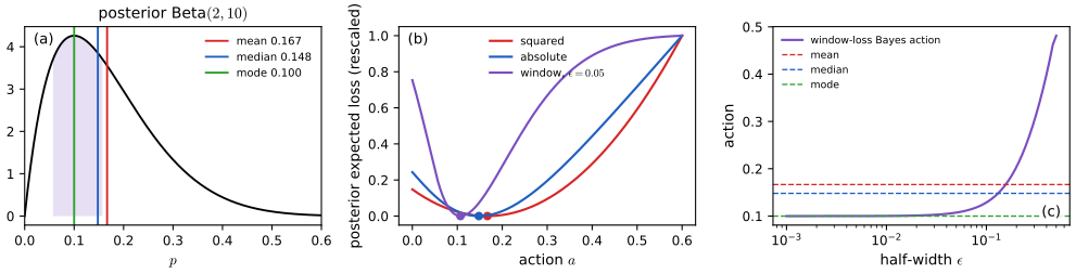
fig_12_s2. Download: PDF · SVGSee also (companion courses): the same three optima for prediction in Result 1.19 of Bayesian and Probabilistic Machine Learning and Result 4.10 of Foundations of Deep Learning, whose Minkowski loss demo follows a different route to "the mode" (the loss \(|a-\th|^q\) with \(q\to0\)), which, as Result 4.11 there shows, does not lead to the mode in general.
Example 12.9. p. 198 Let \(X_1,\dots,X_n\sim\N(\mu,\sigma^2)\) with \(\sigma^2\) known and prior \(\mu\sim\N(a,b^2)\). The Bayes estimator under squared loss is the posterior mean
\[ \ht(X_1,\dots,X_n)=\frac{b^2}{b^2+\frac{\sigma^2}{n}}\,\bX+\frac{\frac{\sigma^2}{n}}{b^2+\frac{\sigma^2}{n}}\,a . \]Filling the gap 12.6: Example 12.9, the posterior and the risks p. 198
The posterior is \(\N(\ht,\tau^2)\) with \(1/\tau^2=n/\sigma^2+1/b^2\). Since it is symmetric and unimodal, \(\ht\) is also the posterior median and mode, so it is the Bayes rule for all three losses of Theorem 12.8. Its Bayes risk is the posterior variance \(\tau^2=\frac{(\sigma^2/n)b^2}{b^2+\sigma^2/n}\), the same for every data set; its frequentist risk, with \(w=b^2/(b^2+\sigma^2/n)\), is
\[ R(\mu,\ht)=w^2\frac{\sigma^2}{n}+(1-w)^2(\mu-a)^2 , \]below \(\sigma^2/n\) near the prior mean and unbounded far from it. As \(b\to\infty\), \(w\to1\) and \(\ht\to\bX\): the sample mean is a limit of Bayes rules, which is how its minimaxity is proved in Theorem 12.A.
Derivation
Since \(\sum_i(x_i-\mu)^2\)
which is the exponent of a Normal density with precision \(1/\tau^2=n/\sigma^2+1/b^2\) and mean \(\tau^2(n\bx/\sigma^2+a/b^2)\); multiplying numerator and denominator by \(b^2\sigma^2/n\) gives the weights \(w\) and \(1-w\). The Bayes risk is \(\int r(\ht\given x)m(x)\,\d x=\tau^2\) by Theorem 12.7 and part (a) of the previous box. For the frequentist risk, \(\ht-\mu=w(\bX-\mu)+(1-w)(a-\mu)\), whose mean is \((1-w)(a-\mu)\) and variance \(w^2\sigma^2/n\). ∎
See also (companion courses): Result 2.16 of Bayesian and Probabilistic Machine Learning (the same posterior, derived in full) and Filling the gap 2.17 of Statistical Methods for Modern Biology (the posterior mean as shrinkage, for a proportion).
12.4 Minimax Rules
p. 198 Minimax rules are hard to find in general; the book gives the key tools, and the message is: a Bayes rule with constant risk is minimax.
Theorem 12.10 (least favourable prior) pp. 198–199
Let \(\ht_f\) be the Bayes rule for a prior \(f\),
\[ r(f,\ht_f)=\inf_{\ht}r(f,\ht), \tag{12.8} \]and suppose that
\[ R(\th,\ht_f)\le r(f,\ht_f)\quad\text{for all }\th. \tag{12.9} \]Then \(\ht_f\) is minimax, and \(f\) is called a least favourable prior.
Proof
Suppose some rule \(\ht_0\) had \(\sup_\th R(\th,\ht_0)<\sup_\th R(\th,\ht_f)\). An average never exceeds a maximum, so
\[ r(f,\ht_0)\le\sup_\th R(\th,\ht_0)<\sup_\th R(\th,\ht_f)\le r(f,\ht_f), \]the last step by (12.9). This contradicts (12.8). ∎
Theorem 12.11 (a Bayes rule with constant risk is minimax) p. 199
If \(\ht\) is the Bayes rule for some prior \(f\) and \(R(\th,\ht)=c\) for all \(\th\), then \(\ht\) is minimax.
Proof
\(r(f,\ht)=\int c\,f(\th)\,\d\th=c\), so \(R(\th,\ht)\le r(f,\ht)\) for all \(\th\), which is (12.9); apply Theorem 12.10. ∎
Filling the gap 12.7: why "least favourable", uniqueness, and limits of Bayes rules pp. 198–199
(a) The prior of Theorem 12.10 is the worst prior for the statistician. Under (12.9), for every prior \(g\) with Bayes rule \(\ht_g\), \(r(g,\ht_g)\le r(f,\ht_f)\): no prior has a larger minimal Bayes risk. Moreover \(\sup_\th R(\th,\ht_f)=r(f,\ht_f)\), so the risk of \(\ht_f\) equals its maximum on the support of \(f\): a least favourable prior sits where the risk is largest (the two atoms of Figure 12.3).
(b) Uniqueness. If \(\ht_f\) is the unique Bayes rule for \(f\) (up to sets of marginal probability zero, as for squared loss, Filling the gap 12.4, item 4), then it is the unique minimax rule.
(c) Theorem 12.A below removes the need for a proper prior.
Proofs of (a) and (b)
(a) \(r(g,\ht_g)\le r(g,\ht_f)\)
(b) If \(\ht'\) is also minimax, \(r(f,\ht')\le\sup_\th R(\th,\ht')\)
Theorem 12.A (limits of Bayes risks; not in the book)
Let \(f_1,f_2,\dots\) be priors with Bayes rules \(\ht_k\) and Bayes risks \(r(f_k,\ht_k)\to c\). If an estimator \(\ht\) satisfies \(\sup_\th R(\th,\ht)\le c\), then \(\ht\) is minimax.
Proof, and the sample mean as an application
For any estimator \(\tth\) and every \(k\), \(\sup_\th R(\th,\tth)\ge r(f_k,\tth)\)
Application. For \(X_1,\dots,X_n\sim\N(\th,1)\) and the priors \(f_k=\N(0,k)\), the Bayes rule is the posterior mean and its Bayes risk is the posterior variance \(\frac{k/n}{k+1/n}\to\frac1n\) (Filling the gap 12.6). Since \(R(\th,\bX)=1/n\) for every \(\th\), \(\bX\) is minimax under squared loss. Theorem 12.11 could not be used directly: \(\bX\) is not the Bayes rule of any proper prior (an unbiased estimator is never a Bayes rule under squared loss with finite Bayes risk, unless it is error-free; Lehmann and Casella 1998, Theorem 4.2.3).
Example 12.12. p. 199 In the Bernoulli model with squared loss, the estimator
\[ \widehat p=\frac{\sum_{i=1}^nX_i+\sqrt{n/4}}{n+\sqrt n} \]has constant risk (Example 12.3) and is the posterior mean, hence the Bayes rule, for the prior \(\Bet(\sqrt{n/4},\sqrt{n/4})\) (a \(\Bet(\alpha,\beta)\) prior gives the posterior \(\Bet(\alpha+Y,\beta+n-Y)\), with mean \((Y+\alpha)/(n+\alpha+\beta)\)). By Theorem 12.11 it is minimax, and by Filling the gap 12.7(b) it is the only minimax estimator. Its maximum risk is \(1/\{4(\sqrt n+1)^2\}\).
Example 12.13. p. 199 Keep the Bernoulli model but change the loss to
\[ L(p,\widehat p)=\frac{(p-\widehat p)^2}{p(1-p)} , \]which measures the error relative to the variance of a single observation. For \(\widehat p=\bX\) the risk is \(\frac1{p(1-p)}\cdot\frac{p(1-p)}n=\frac1n\), constant in \(p\). The book states that \(\bX\) is the Bayes rule for this loss and the uniform prior, so \(\bX\) is minimax.
Filling the gap 12.8: Bayes rules for the weighted loss of Example 12.13 p. 199
For a loss \(w(p)(p-a)^2\) the posterior risk is a weighted posterior second moment, so the Bayes action is the mean of the reweighted posterior \(\propto w(p)f(p\given y)\). With the uniform prior and \(w=1/\{p(1-p)\}\), the reweighted posterior is \(\Bet(y,n-y)\), whose mean is \(y/n\); at \(y=0\) and \(y=n\) the only action with finite posterior risk is \(y/n\) itself. So \(\bX\) is the Bayes rule; with constant risk \(1/n\) it is minimax (Theorem 12.11), and uniquely so (Filling the gap 12.7(b)).
More generally, for a \(\Bet(a_0,b_0)\) prior with \(a_0,b_0\ge1\) the Bayes rule is \((Y+a_0-1)/(n+a_0+b_0-2)\). And under this loss the estimator \((Y+\alpha)/(n+\alpha+\beta)\) has risk
\[ R(p)=\frac{n-s^2+\alpha^2/p+\beta^2/(1-p)}{(n+s)^2},\qquad s=\alpha+\beta, \]which is unbounded unless \(\alpha=\beta=0\): every pseudo-count estimator, including the squared-loss minimax rule of Example 12.12, has infinite maximum risk here. The loss decides what "best" means.
Derivations
If \(\int w(p)f(p\given y)\,\d p<\infty\), let \(f_w(p\given y)=w(p)f(p\given y)/\int wf\). Then \(\int w(p)(p-a)^2f(p\given y)\,\d p\)
For a \(\Bet(a_0,b_0)\) prior, \(wf\propto p^{y+a_0-2}(1-p)^{n-y+b_0-2}\), with mean \((y+a_0-1)/(n+a_0+b_0-2)\) when both exponents exceed \(-1\) (the boundary cases with \(a_0=1\) or \(b_0=1\) are handled as above).
For the risk, use \(R=\{np(1-p)+(\alpha-sp)^2\}/\{(n\)
p. 199 What is the minimax estimator of a Normal mean?
Theorem 12.14 (the sample mean is minimax) p. 200
Let \(X_1,\dots,X_n\sim\N(\th,1)\) and \(\ht=\bX\). Then \(\ht\) is minimax for every "well-behaved" loss, meaning a loss \(L(\ht-\th)\) whose sublevel sets are convex and symmetric about the origin, and it is the only estimator with this property (up to sets of measure zero).
Filling the gap 12.9: proof of Theorem 12.14 in one dimension p. 200
In one dimension a convex symmetric sublevel set is an interval \([-c,c]\) (or its interior), so "well-behaved" means \(L(z)=L(-z)\) and \(L\) is nondecreasing in \(|z|\); assume also that \(L\) is continuous. The proof combines Theorem 12.A with a one-dimensional form of Anderson's lemma (Anderson, 1955): if \(Z\) has a density that is symmetric about 0 and nonincreasing in \(|z|\), then \(\P(|Z-a|\le c)\le\P(|Z|\le c)\) for all \(a\) and \(c\), and hence \(\E L(Z-a)\ge\E L(Z)\).
Uniqueness for squared loss follows from admissibility (Theorem 12.20) and strict convexity. In dimension \(k\ge3\) uniqueness fails: the James-Stein estimator also has maximum risk \(k\) (Section 12.7).
Proof
Anderson's lemma in one dimension. Let \(g\) be the density of \(Z\). Then \(\frac{\d}{\d a}\P(|Z-a|\le c)\)
Bayes risks. \(\bX\) is sufficient and \(\bX\sim\N(\th,1/n)\). Under the prior \(\N(0,k)\) the posterior is \(\N(w\bx,\tau_k^2)\) with \(\tau_k^2=\frac{k/n}{k+1/n}\) (Filling the gap 12.6). By Anderson's lemma, applied to the symmetric unimodal posterior, the posterior risk \(\E[L(a-\th)\given\bx]\) is minimised at the posterior mean, with value \(\E L(\tau_kZ)\), \(Z\sim\N(0,1)\). So the Bayes risk is \(r_k=\E L(\tau_kZ)\).
The limit. As \(k\to\infty\), \(\tau_k\uparrow n^{-1/2}\), and \(L(\tau Z)\) is nondecreasing in \(\tau\) and continuous, so by monotone convergence \(r_k\uparrow\E L(Z/\sqrt n)\), which is exactly \(R(\th,\bX)\) for every \(\th\) (because \(\bX-\th\sim\N(0,1/n)\)). Theorem 12.A gives minimaxity.
Uniqueness (squared loss). Let \(\ht'\) be minimax, so \(\sup_\th R(\th,\ht')=1/n\), and let \(\bar\th=\tfrac12(\bX+\ht')\). By convexity \((\bar\th-\th)^2\)
p. 200 If the parameter space is restricted, Theorem 12.14 fails, as the next example shows.
Example 12.15. p. 200 Let \(X\sim\N(\th,1)\) where \(\th\) is known to lie in \([-m,m]\), \(0<m<1\). Under squared loss the unique minimax estimator is
\[ \ht(X)=m\tanh(mX),\qquad\tanh(z)=\frac{e^z-e^{-z}}{e^z+e^{-z}} . \]It is the Bayes rule for the prior putting mass 1/2 at each of \(-m\) and \(m\); its risk is not constant, but it satisfies \(R(\th,\ht)\le r(f,\ht)\) for all \(\th\) (Figure 12.3), so Theorem 12.10 applies.
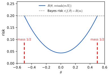
fig_12_3. Download: PDF · SVGFilling the gap 12.10: Example 12.15 in full p. 200
(a) The Bayes rule. For the two-point prior, \(\P(\th=m\given x)=e^{mx}/(e^{mx}+e^{-mx})\), so the posterior mean is \(m\tanh(mx)\); it is the unique Bayes rule (squared loss).
(b) Condition (12.9). The risk \(R(\th)=\E\{m\tanh(m(\th+Z))-\th\}^2\), \(Z\sim\N(0,1)\), is even in \(\th\), so the Bayes risk is \(r=\tfrac12R(m)+\tfrac12R(-m)=R(m)\), and (12.9) says: \(R(\th)\le R(m)\) on \([-m,m]\).
(c) A proof of (12.9) for \(m\le0.668\). There \(R\) is convex: \(R''(\th)\)
(d) Beyond the convexity range. The convexity bound fails for \(m>0.668\), but (12.9) still holds, now by computation: \(\max_{|\th|\le m}R(\th)=R(m)\) for every \(m\) up to \(m_0=1.0567\), where \(R(0)\) overtakes \(R(m)\) (Figure 12.S3). For \(m>m_0\) the two-point prior is no longer least favourable and the minimax rule is the Bayes rule of a prior with more support points (Casella and Strawderman, 1981). The book's condition \(m<1\) is a convenient sufficient condition.
(e) Uniqueness follows from (a) and Filling the gap 12.7(b). With \(m=0.5\) the minimax risk is 0.1990, a fifth of the risk of \(X\): knowing that \(|\th|\le0.5\) is worth a lot.
Proofs
(a) \(\phi(x\mp m)=\phi(x)e^{\pm mx-m^2/2}\), so \(\P(\th=m\given x)=\frac{e^{mx}}{e^{mx}+e^{-mx}}\) and the posterior mean is \(m\frac{e^{mx}-e^{-mx}}{e^{mx}+e^{-mx}}\).
(b) Replacing \(Z\) by \(-Z\) (same distribution) and using that \(\tanh\) is odd, \(R(-\th)=\E\{-m\tanh(m(\th+Z))+\th\}^2\)
(c) Let \(g(x)=m\tanh(mx)\). Then \(g'(x)=m^2\sech^2(mx)\in(0,m^2]\) and \(g''(x)=-2m^3\sech^2(mx)\tanh(mx)\). With \(u=\tanh(mx)\), \(|\sech^2\tanh|=(1-u^2)|u|\le\frac{2}{3\sqrt3}\) (maximum at \(u^2=1/3\)), so \(|g''|\le\frac{4m^3}{3\sqrt3}\). All derivatives are bounded, so we may differentiate under the expectation:
\[ R''(\th)=2\,\E\big[(g'(\th+Z)-1)^2+(g(\th+Z)-\th)\,g''(\th+Z)\big]. \]Since \(0<g'\le m^2<1\), \((1-g')^2\ge(1-m^2)^2\); and \(|g-\th|\le|g|+|\th|\le2m\). Hence \(R''(\th)\)
(d) \(R\) is computed by 120-point Gauss-Hermite quadrature (accurate to about \(10^{-14}\)) on a fine grid of \(\th\) and \(m\); \(m_0\) is the root of \(R(0)=R(m)\). ∎
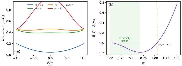
fig_12_s3. Download: PDF · SVG12.5 Maximum Likelihood, Minimax, and Bayes
p. 201 In parametric models satisfying weak regularity conditions, the MLE is approximately minimax. Under squared loss the risk is variance plus squared bias, and in large samples the variance dominates (typically the squared bias is \(O(n^{-2})\) and the variance \(O(n^{-1})\)), so \(R(\th,\ht)\approx\V_\th(\ht)\approx1/\{nI(\th)\}\), \(I\) being the Fisher information (Chapter 9 of the book):
\[ nR(\th,\ht)\approx\frac1{I(\th)}. \tag{12.10} \]No other estimator does better in a local, large-sample sense: for every estimator \(\tth_n\),
\[ \lim_{\epsilon\to0}\ \limsup_{n\to\infty}\ \sup_{|\th'-\th|<\epsilon}\ nR(\th',\tth_n)\ \ge\ \frac1{I(\th)}. \tag{12.11} \]The MLE is also approximately the Bayes rule. In summary: in most parametric models, with large samples, the MLE is approximately minimax and Bayes. (In the book the arbitrary estimator in (12.11) is called \(\ht\) and the nearby parameter value \(\th'\), after the text has used \(\th'\) for the estimator; see the notes on the book.)
Filling the gap 12.11: why the bound must be local, and a proof of (12.11) p. 201
(a) Superefficiency. The text says that "for large \(n\), \(R(\th,\th')\ge R(\th,\ht)\)" for any other estimator \(\th'\). Taken pointwise this is false. For \(X_1,\dots,X_n\sim\N(\th,1)\), Hodges' estimator (reported by Le Cam, 1953)
\[ \tth_n=\bX\,\ind\{|\bX|>n^{-1/4}\} \]has \(nR(\th,\tth_n)\to1=1/I(\th)\) for every \(\th\ne0\) but \(nR(0,\tth_n)\to0\): it beats the MLE at \(\th=0\) for all large \(n\). The price is paid nearby: \(\sup_\th nR(\th,\tth_n)\) grows like \(\sqrt n\) (5.6, 69 and 858 for \(n=10^2,10^4,10^6\)), attained near \(\th\approx0.9\,n^{-1/4}\) (Figure 12.S4(a)). The supremum over a shrinking neighbourhood in (12.11) is what rules such estimators out.
(b) The van Trees inequality (Theorem 12.B below) is a Bayesian version of the Cramér-Rao bound that holds for every estimator, biased or not.
(c) Proof of (12.11). In a regular model with \(I\) continuous at \(\th\), for every estimator \(\tth_n\), every \(n\) and every \(\epsilon>0\),
\[ \sup_{|\th'-\th|<\epsilon}nR(\th',\tth_n)\ \ge\ \frac{n}{n\sup_{|\th'-\th|\le\epsilon}I(\th')+\pi^2/\epsilon^2}, \]whose right side tends to \(1/\sup_{|\th'-\th|\le\epsilon}I(\th')\) as \(n\to\infty\) and then to \(1/I(\th)\) as \(\epsilon\to0\). This proves (12.11) even with \(\liminf\) in place of \(\limsup\). In the Normal model with \(\epsilon=0.5\) the bound is 0.20 at \(n=10\), 0.72 at \(n=100\) and 0.996 at \(n=10^4\) (Figure 12.S4(b)).
Derivations
(a) Let \(t=n^{-1/4}\), \(s=n^{-1/2}\), \(a=(-t-\th)/s\), \(b=(t-\th)/s\) and \(P=\Phi(b)-\Phi(a)=\P_\th(|\bX|\le t)\). With \(\bX=\th+sZ\), the estimator equals \(\bX\) off the event \(\{a\le Z\le b\}\) and 0 on it, so
\[ nR(\th,\tth_n)=\E\big[Z^2\ind\{Z\notin[a,b]\}\big]+n\th^2P=1-\big(P-b\phi(b)+a\phi(a)\big)+n\th^2P, \]using \(\E[Z^2\ind\{a\le Z\le b\}]\)
(c) Take the prior density \(\lambda(\th')\)
Multiply by \(n\) and take limits; continuity of \(I\) gives the last step. ∎
Theorem 12.B (van Trees inequality; Gill and Levit, 1995)
Let \(\lambda\) be a prior density on \([c,d]\), continuously differentiable on \((c,d)\), with \(\lambda(c)=\lambda(d)=0\) and \(J(\lambda)=\int\lambda'(\th)^2/\lambda(\th)\,\d\th<\infty\). Suppose the model \(f_n(x;\th)\) for the whole sample has a score \(s_\th(x)=\partial_\th\log f_n(x;\th)\) with \(\E_\th s_\th=0\) and \(\E_\th s_\th^2=nI(\th)\), and that \(\partial_\th\{f_n(x;\th)\lambda(\th)\}\) may be integrated in \(\th\) as a derivative. Then every estimator \(\tth\) satisfies
\[ \int\E_\th(\tth-\th)^2\,\lambda(\th)\,\d\th\ \ge\ \frac{1}{n\int I(\th)\lambda(\th)\,\d\th+J(\lambda)} . \]Proof
Let \(p(x,\th)=f_n(x;\th)\lambda(\th)\) be the joint density and \(\psi=\partial_\th\log p=s_\th(x)+\lambda'(\th)/\lambda(\th)\). For fixed \(x\), integrate by parts in \(\th\):
\[ \int_c^d(\tth(x)-\th)\,\partial_\th p(x,\th)\,\d\th=\Big[(\tth(x)-\th)p(x,\th)\Big]_c^d+\int_c^dp(x,\th)\,\d\th=\int_c^dp(x,\th)\,\d\th, \]since \(\lambda\) vanishes at both ends. Integrating over \(x\) gives \(\E[(\tth-\th)\psi]=1\) under the joint distribution. By the Cauchy-Schwarz inequality (Theorem 4.8), \(1\le\E[(\tth-\th)^2]\,\E[\psi^2]\). Finally \(\E\psi^2=\E[s_\th^2]+2\E[s_\th\lambda'/\lambda]\)
Filling the gap 12.12: the MLE is approximately the Bayes rule p. 201
For Bernoulli data and any fixed \(\Bet(\alpha,\beta)\) prior, the posterior mean and the MLE differ by at most \(\max(\alpha,\beta)/(n+\alpha+\beta)\) whatever the data, which is \(O(1/n)\), an order smaller than their standard error \(O(n^{-1/2})\). Their scaled risks agree to first order: \(nR(p,\widehat p_{\rm Bayes})\)
Derivation
With \(s=\alpha+\beta\) and \(\widehat p=Y/n\in[0,1]\): \(\frac{Y+\alpha}{n+s}-\frac Yn=\frac{n\alpha-sY}{n(n+s)}\)
p. 201 The caveat: these results break down when the number of parameters is large.
Example 12.16 (many Normal means). pp. 201–202 Let \(Y_i\sim\N(\th_i,\sigma^2/n)\), \(i=1,\dots,n\), independently, with \(\th=(\th_1,\dots,\th_n)\) in the ball
\[ \Theta_n=\Big\{\th:\ \sum_{i=1}^n\th_i^2\le c^2\Big\} \]for some \(c>0\): as many parameters as observations, a model to which many nonparametric problems are equivalent. The MLE is \(\ht=Y\), and under the loss \(L(\th,\ht)=\sum_i(\ht_i-\th_i)^2\) its risk is \(n\cdot\sigma^2/n=\sigma^2\). The minimax risk is smaller, and an estimator achieving it can be written down, so maximum likelihood is not optimal in high dimensions. The book gives the minimax risk as approximately \(\sigma^2/(\sigma^2+c^2)\); the correct value is \(\sigma^2c^2/(\sigma^2+c^2)\) (next box and the notes on the book).
Filling the gap 12.13: the minimax risk for many Normal means is \(\sigma^2c^2/(\sigma^2+c^2)\) p. 202
Let \(R_n^*=\inf_{\ht}\sup_{\th\in\Theta_n}R(\th,\ht)\). Then (Pinsker, 1980, in this form)
\[ R_n^*\le\frac{\sigma^2c^2}{\sigma^2+c^2}\ \text{ for every }n,\qquad R_n^*\to\frac{\sigma^2c^2}{\sigma^2+c^2}\ \text{ as }n\to\infty . \](a) Upper bound. The linear estimator \(bY\) with \(b=c^2/(\sigma^2+c^2)\) has maximum risk exactly \(\sigma^2c^2/(\sigma^2+c^2)\) over \(\Theta_n\).
(b) Lower bound. For every \(\delta\in(0,1)\), \(\liminf_nR_n^*\)
(c) James-Stein attains it without knowing \(c\). The James-Stein estimator \(\big(1-\frac{(n-2)\sigma^2/n}{\|Y\|^2}\big)Y\) of Section 12.7 has \(\sup_{\Theta_n}R\)
Proofs
(a) \(\E\|bY-\th\|^2\)
(b) Reduction. Let \(\Pi\) be the Euclidean projection onto the closed convex set \(\Theta_n\). For \(\th\in\Theta_n\), \(\|\Pi(v)-\th\|\le\|v-\th\|\) (projections onto convex sets do not increase distances to points of the set), so replacing any estimator by its projection never increases the risk on \(\Theta_n\). Hence it suffices to bound \(\sup_{\Theta_n}R\) for estimators with values in \(\Theta_n\), for which the loss is at most \((\|\ht\|+\|\th\|)^2\)
Bayes risk. Under the prior \(\pi\): \(\th_i\) independent \(\N(0,\tau^2)\), \(\tau^2=(1-\delta)c^2/n\), each coordinate is the Normal-Normal problem of Filling the gap 12.6, with posterior variance \(\frac{(\sigma^2/n)\tau^2}{\sigma^2/n+\tau^2}\). Summing over \(n\) coordinates, every estimator has Bayes risk at least \(B_\delta=\frac{\sigma^2(1-\delta)c^2}{\sigma^2+(1-\delta)c^2}\).
Truncation. For an estimator with values in \(\Theta_n\), split the Bayes risk over \(\Theta_n\) and its complement:
\[ B_\delta\le\int R\,\d\pi\le\sup_{\Theta_n}R+\E_\pi\big[(2c^2+2\|\th\|^2)\ind\{\|\th\|^2>c^2\}\big]. \]Under \(\pi\), \(\|\th\|^2=\tau^2\chi^2_n\) has mean \((1-\delta)c^2\) and variance \(2(1-\delta)^2c^4/n\). By Cauchy-Schwarz and Chebyshev (Theorem 4.2), the last term is at most \(\{\E(2c^2\)
(c) Rescale \(X_i=\sqrt nY_i/\sigma\sim\N(\sqrt n\th_i/\sigma,1)\); the estimator is James-Stein for \(X\) multiplied back by \(\sigma/\sqrt n\), so by Filling the gap 12.17 its risk is \(\frac{\sigma^2}{n}\big(n-(n\)
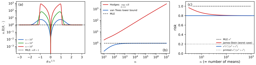
fig_12_s4. Download: PDF · SVG12.6 Admissibility
p. 202 Minimax and Bayes estimators are good in the sense of small risk. It is also useful to say what makes an estimator bad.
Definition 12.17 (admissibility) p. 202
An estimator \(\ht\) is inadmissible if there is a rule \(\ht'\) with \(R(\th,\ht')\le R(\th,\ht)\) for all \(\th\) and \(R(\th,\ht')<R(\th,\ht)\) for at least one \(\th\). Otherwise \(\ht\) is admissible.
Example 12.18. p. 202 For \(X\sim\N(\th,1)\) and squared loss, the constant \(\ht=3\) is admissible. If \(\ht'\) were at least as good everywhere, then \(R(3,\ht')\le R(3,\ht)=0\), so \(\int(\ht'(x)-3)^2f(x;3)\,\d x=0\) and \(\ht'=3\): nothing beats it. Admissible, and still a bad rule. (Fine print: \(\ht'(x)=3\) for almost every \(x\), and since all \(\N(\th,1)\) distributions have the same null sets, \(\ht'\) and \(\ht\) have the same risk at every \(\th\).)
Theorem 12.19 (Bayes rules are admissible) pp. 202–203
Let \(\Theta\subset\R\), and suppose that \(\th\mapsto R(\th,\ht)\) is continuous for every \(\ht\). Let \(f\) be a prior density with full support: \(\int_{\th-\epsilon}^{\th+\epsilon}f>0\) for every \(\th\) and \(\epsilon>0\). If the Bayes rule \(\ht_f\) has finite Bayes risk, it is admissible.
Proof
Suppose \(\ht\) dominates \(\ht_f\): \(R(\th,\ht)\le R(\th,\ht_f)\) for all \(\th\), with \(\nu=R(\th_0,\ht_f)-R(\th_0,\ht)>0\) at some \(\th_0\). By continuity there is \(\epsilon>0\) with \(R(\th,\ht_f)-R(\th,\ht)>\nu/2\) on \((\th_0-\epsilon,\th_0+\epsilon)\). The Bayes risk of \(\ht\) is finite too (it is at most that of \(\ht_f\)), so we may subtract:
\[ r(f,\ht_f)-r(f,\ht)=\int\big(R(\th,\ht_f)-R(\th,\ht)\big)f(\th)\,\d\th\ge\int_{\th_0-\epsilon}^{\th_0+\epsilon}\big(R(\th,\ht_f)-R(\th,\ht)\big)f(\th)\,\d\th\ge\frac\nu2\int_{\th_0-\epsilon}^{\th_0+\epsilon}f>0, \]the first inequality because the integrand is nonnegative everywhere. So \(\ht_f\) does not minimise the Bayes risk: a contradiction. ∎
Filling the gap 12.14: the hypotheses of Theorem 12.19 pp. 202–203
Continuity of risk is automatic in exponential families (Normal, Bernoulli, Poisson, ...): for any estimator, \(\th\mapsto R(\th,\ht)\) is continuous, indeed analytic in the natural parameter, on the interior of the set where it is finite in a neighbourhood (Lehmann and Casella, 1998, Theorem 1.5.8).
Finite Bayes risk is essential: the "flat prior" on \(\R^k\) produces the formal Bayes rule \(X\), which is inadmissible for \(k\ge3\) (Section 12.7); the proof fails because every rule has infinite "Bayes risk", so the subtraction above is meaningless.
Full support can be traded for uniqueness. If \(\ht_f\) is the unique Bayes rule for \(f\) (up to sets of marginal probability zero, e.g. squared loss, Filling the gap 12.4, item 4) and has finite Bayes risk, it is admissible, whatever the support of \(f\) and without continuity. This is the cleanest route for Examples 12.12 and 12.15.
Proof of the last statement
If \(\ht\) dominates \(\ht_f\), then \(r(f,\ht)\le r(f,\ht_f)\), so \(\ht\) is also Bayes for \(f\), hence equal to \(\ht_f\) almost surely under the marginal. The risk functions then agree at every \(\th\) whose sampling distribution is dominated by the marginal (in particular at every \(\th\) in the support of \(f\) in the models of this chapter, where all \(\P_\th\) share the same null sets), so \(\ht\) is not strictly better anywhere. ∎
Theorem 12.20 (the sample mean is admissible) p. 203
Let \(X_1,\dots,X_n\sim\N(\mu,\sigma^2)\). Under squared loss, \(\bX\) is admissible.
p. 203 The book omits the proof and sketches an idea: posterior means under strictly positive priors are admissible, and as \(b^2\to\infty\) the posterior mean under the prior \(\N(a,b^2)\) tends to \(\bX\).
Filling the gap 12.15: a proof of Theorem 12.20 p. 203
The sketch is not a proof. A limit of admissible estimators need not be admissible: in \(\R^k\), \(k\ge3\), the posterior means \(\frac{b^2}{1+b^2}X\) under \(\N(0,b^2I)\) priors are admissible (unique Bayes rules), they converge to \(X\) as \(b\to\infty\), and \(X\) is inadmissible (Section 12.7). A quantitative argument is needed. Two classical ones exist: Blyth's method (Filling the gap 12.18, which also covers dimension 2) and the information inequality method of Hodges and Lehmann (1951), given here.
Reduction to known \(\sigma\). If some \(\ht\) dominated \(\bX\) over all \((\mu,\sigma)\), strictly at \((\mu_0,\sigma_0)\), then in the model with \(\sigma=\sigma_0\) known, \(\ht\) would dominate \(\bX\) strictly at \(\mu_0\). So assume \(\sigma\) known and let \(v=\sigma^2/n=R(\mu,\bX)\).
Claim. If \(R(\mu,\ht)\le v\) for all \(\mu\), then \(R(\mu,\ht)=v\) for all \(\mu\). Hence nothing improves on \(\bX\) anywhere.
Proof
Information inequality. Since \(R(\mu,\ht)\le v\), \(\E_\mu\ht^2<\infty\) for every \(\mu\). In an exponential family such expectations are differentiable in \(\mu\) under the integral sign (Lehmann and Casella, 1998, Theorem 1.5.8), so the bias \(b(\mu)=\E_\mu\ht-\mu\) is differentiable and \(\frac{\d}{\d\mu}\E_\mu\ht=\Cov_\mu(\ht,S)\), where \(S=n(\bX-\mu)/\sigma^2\) is the score, with \(\V_\mu S=1/v\). Cauchy-Schwarz gives \((1+b'(\mu))^2\le\V_\mu(\ht)/v\). Therefore
\[ v\ \ge\ R(\mu,\ht)=b(\mu)^2+\V_\mu(\ht)\ \ge\ b(\mu)^2+v\,(1+b'(\mu))^2 . \tag{$*$} \]Consequences for the bias. From \((*)\), \((1+b')^2\le1\), so \(-2\le b'\le0\): \(b\) is nonincreasing. Also \(b^2\le v\{1-(1+b')^2\}\)
The bias is zero. Suppose \(b(\mu_0)<0\). For \(\mu>\mu_0\), \(b(\mu)\le b(\mu_0)<0\), and \(\frac{\d}{\d\mu}\frac1{b}=-\frac{b'}{b^2}\ge\frac1{2v}\); integrating, \(\frac1{b(\mu)}\ge\frac1{b(\mu_0)}+\frac{\mu-\mu_0}{2v}\), which is positive for large \(\mu\), impossible since \(b(\mu)<0\). If \(b(\mu_0)>0\), the same argument for \(\mu<\mu_0\) gives \(\frac1{b(\mu)}\le\frac1{b(\mu_0)}-\frac{\mu_0-\mu}{2v}\), negative for \(\mu\) far to the left, impossible since \(b(\mu)\ge b(\mu_0)>0\). So \(b\equiv0\), hence \(b'\equiv0\), and \((*)\) gives \(R(\mu,\ht)\ge v\); with \(R\le v\), equality holds everywhere. ∎
p. 203 A rule can be minimax, admissible, both or neither, but there are links.
Theorem 12.21 (constant risk and admissible implies minimax) p. 203
If \(\ht\) has constant risk and is admissible, it is minimax.
Proof
Let \(R(\th,\ht)=c\). If \(\ht\) were not minimax there would be a rule \(\ht'\) with \(R(\th,\ht')\le\sup_\th R(\th,\ht')<c\)
Theorem 12.22 (the Normal mean, squared loss) p. 203
If \(X_1,\dots,X_n\sim\N(\th,1)\), then \(\ht=\bX\) is minimax under squared loss.
Proof
\(\bX\) is admissible (Theorem 12.20) and has constant risk \(1/n\); apply Theorem 12.21. (A second proof, by limits of Bayes risks, is the application of Theorem 12.A.) ∎
Definition 12.B (strong inadmissibility) p. 204
\(\ht\) is strongly inadmissible if there are a rule \(\ht'\) and an \(\epsilon>0\) with \(R(\th,\ht')<R(\th,\ht)-\epsilon\) for all \(\th\).
Theorem 12.23 (minimax rules are close to admissible) p. 204
If \(\ht\) is minimax (with finite maximum risk), it is not strongly inadmissible.
Filling the gap 12.16: proof of Theorem 12.23, and why "finite" is needed p. 204
The book states Theorem 12.23 without proof (and without the finiteness condition, which is needed). Minimax rules can be inadmissible: in \(\R^k\), \(k\ge3\), \(X\) is minimax (constant risk \(k\), and the argument of Theorem 12.A with \(\N(0,bI)\) priors) but dominated by James-Stein (Section 12.7). The improvement there is not uniform (the James-Stein risk tends to \(k\) as \(\|\th\|\to\infty\)), exactly as Theorem 12.23 requires.
Proof and counterexample
Let \(M=\sup_\th R(\th,\ht)<\infty\). If \(R(\th,\ht')<R(\th,\ht)-\epsilon\le M-\epsilon\) for all \(\th\), then \(\sup_\th R(\th,\ht')\le M-\epsilon<M\), contradicting minimaxity of \(\ht\). ∎
Without \(M<\infty\) the statement fails: for \(\N(\mu,\sigma^2)\) data with both parameters unknown and squared loss, every estimator has infinite maximum risk (its risk is at least the minimax risk \(\sigma^2/n\) of the known-\(\sigma\) problem), so every estimator is minimax, including \(\bX+1\), which is strongly inadmissible: \(R(\cdot,\bX)=R(\cdot,\bX+1)-1\).
12.7 Stein's Paradox
p. 204 For \(X\sim\N(\th,1)\) and squared loss, \(\ht(X)=X\) is admissible (Theorem 12.20 with \(n=1\)). For two unrelated means, \(X_j\sim\N(\th_j,1)\), \(j=1,2\), independent, with loss \(\sum_j(\ht_j-\th_j)^2\), \(X=(X_1,X_2)\) is again admissible. Now take \(k\) means, \(X_j\sim\N(\th_j,1)\) independent, loss \(L(\th,\ht)=\sum_{j=1}^k(\ht_j-\th_j)^2\). Stein (1956) proved the astonishing fact that for \(k\ge3\) the estimator \(X\) is inadmissible. The James-Stein estimator \(\ht^S=(\ht^S_1,\dots,\ht^S_k)\),
\[ \ht^S_i(X)=\Big(1-\frac{k-2}{\sum_iX_i^2}\Big)^+X_i , \tag{12.12} \]has smaller risk at every \(\th\). It shrinks the observations towards 0. The lesson: when many parameters are estimated together, shrinkage pays, an idea at the heart of modern nonparametric function estimation.
Lemma 12.C (Stein's lemma; Stein, 1981)
Let \(X\sim\N(\th,I_k)\) and let \(g:\R^k\to\R^k\) be weakly differentiable with \(\E|\partial_ig_i(X)|<\infty\) for each \(i\). Then
\[ \E\big[(X-\th)^\T g(X)\big]=\E\Big[\sum_{i=1}^k\partial_ig_i(X)\Big]. \]Proof
One dimension. Let \(Z\sim\N(\mu,1)\) and \(h\) absolutely continuous with \(\E|h'(Z)|<\infty\). Write \(h(z)-h(\mu)=\int_\mu^zh'(t)\,\d t\). For \(t>\mu\), \(\E[(Z-\mu)\ind\{Z>t\}]\)
\(k\) dimensions. Apply this to \(x_i\mapsto g_i(x)\) with the other coordinates held fixed (they are independent of \(X_i\)), take expectations over them, and sum over \(i\). ∎
See also (companion course): the same lemma gives the degrees of freedom of a fit in Result 3.20 of Statistical Learning: Theory and Methods.
Theorem 12.D (the James-Stein estimator dominates \(X\) for \(k\ge3\); James and Stein, 1961)
Let \(X\sim\N(\th,I_k)\), \(k\ge3\), \(\lambda=\|\th\|^2\). The estimator without the positive part, \(\ht^{JS}=\big(1-\frac{k-2}{\|X\|^2}\big)X\), has risk
\[ R(\th,\ht^{JS})=k-(k-2)^2\,\E\frac{1}{\|X\|^2}=k-(k-2)^2\,\E\frac1{k-2+2K},\qquad K\sim\Pois(\lambda/2), \]which is smaller than \(k=R(\th,X)\) for every \(\th\), equals 2 at \(\th=0\) for every \(k\), and tends to \(k\) as \(\|\th\|\to\infty\). The positive-part estimator (12.12) has strictly smaller risk still, at every \(\th\).
Filling the gap 12.17: proof of Theorem 12.D, and the exact risk of (12.12) p. 204
The book quotes Stein's result; here is the proof, in three steps: Stein's lemma turns the risk into an expectation that does not involve \(\th\) explicitly; a Poisson mixture evaluates it; a reflection argument handles the positive part. The positive-part risk also has a closed form: with \(W=\|X\|^2\), \(c=k-2\), \(\nu=k+2K\) and \(Q_\nu(c)=\P(\chi^2_\nu>c)\),
\[ R(\th,\ht^S)=\lambda+\E\Big[\big(2k-W-\tfrac{c^2}{W}\big)\ind\{W>c\}\Big]=\lambda+\E\Big[2kQ_\nu(c)-\nu Q_{\nu+2}(c)-\frac{c^2Q_{\nu-2}(c)}{\nu-2}\Big]. \]Values: at \(\th=0\) the positive part has risk 1.603 (\(k=3\)), 1.258 (\(k=10\)) and 1.076 (\(k=100\)), against 2 for James-Stein and \(k\) for \(X\); for \(k=10\), \(\|\th\|=2\): 10, 4.376 and 3.980.
Proof
Step 1 (risk by Stein's lemma). Write \(\ht^{JS}=X-g(X)\) with \(g(x)=cx/\|x\|^2\). Then \(\partial_i\{x_i/\|x\|^2\}\)
and \(c=k-2\) (the minimiser of \(c^2-2c(k-2)\)) gives \(k-(k-2)^2\E\|X\|^{-2}\), which is below \(k\) since \(0<\E\|X\|^{-2}<\infty\). Any \(c\in(0,2(k-2))\) also dominates \(X\).
Step 2 (Poisson mixture). \(W=\|X\|^2\) is noncentral chi-square with \(k\) degrees of freedom and noncentrality \(\lambda\), which is a \(\chi^2_{k+2K}\) variable with \(K\sim\Pois(\lambda/2)\) (compare moment generating functions). Since \(\E[1/\chi^2_\nu]=1/(\nu-2)\), \(\E[1/W]=\E[1/(k-2+2K)]\). At \(\th=0\), \(K=0\) and the risk is \(k-(k-2)=2\); as \(\lambda\to\infty\), \(K\to\infty\) in probability and the risk tends to \(k\).
Step 3 (the positive part is better). Let \(B=c/W\). The two estimators agree when \(B\le1\). When \(B>1\), \(\ht^S=0\) and
\[ \|\ht^{JS}-\th\|^2-\|\ht^S-\th\|^2=(1-B)^2W-2(1-B)\th^\T X=(1-B)^2W+2(B-1)\th^\T X. \]The first term is positive on \(\{B>1\}\), an event of positive probability. For the second, \((B-1)\ind\{B>1\}=h(\|X\|)\) for a nonnegative function \(h\), and \(\E[h(\|X\|)\th^\T X]\ge0\) for every such \(h\): let \(\rho\) be the reflection across the hyperplane orthogonal to \(\th\), so \(\|\rho x\|=\|x\|\) and \(\th^\T\rho x=-\th^\T x\). The density of \(X\) is proportional to \(e^{\th^\T x-\|x\|^2/2}\), so pairing \(x\) with \(\rho x\),
\[ \E[h(\|X\|)\th^\T X]=\int_{\th^\T x>0}h(\|x\|)\,(\th^\T x)\,\big(p(x)-p(\rho x)\big)\,\d x\ge0,\qquad\frac{p(x)}{p(\rho x)}=e^{2\th^\T x}>1 . \]Hence \(R(\th,\ht^S)<R(\th,\ht^{JS})\) for every \(\th\).
Step 4 (exact positive-part risk). For \(\ht=h(W)X\) with \(h\) Lipschitz, \(\E\|hX-\th\|^2\)
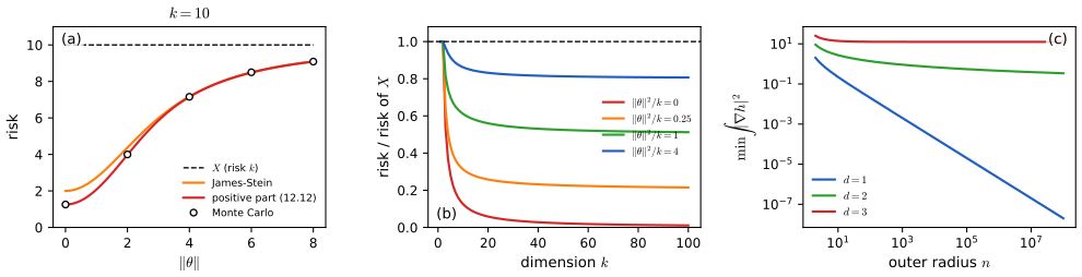
fig_12_s5. Download: PDF · SVGFilling the gap 12.18: why the threshold is three dimensions p. 204
The book says that \(X\) is "not surprisingly" admissible for two means; the proof is in fact delicate, and it shows where three dimensions become different. Let \(X\sim\N(\th,I_d)\), squared loss, so \(R(\th,X)=d\).
Blyth's method (Blyth, 1951). Suppose that for every ball \(B\) there are finite measures \(\pi_n\) (priors that need not be normalised) with Bayes rules \(\delta_n\), such that \(\pi_n(B)\ge c_B\) for a constant \(c_B>0\) and \(\Delta_n=r(\pi_n,X)-r(\pi_n,\delta_n)\to0\). Then \(X\) is admissible.
An energy bound. If \(\pi=h^2\) with \(h\ge0\) smooth and compactly supported, then
\[ \Delta=r(\pi,X)-r(\pi,\delta_\pi)\le4\int_{\R^d}|\nabla h(\th)|^2\,\d\th . \]The three cases. With \(h_n=1\) on the unit ball and 0 beyond radius \(n\) (for another ball, translate and rescale the profile, which changes the energy by a constant factor), the smallest energy is \(2/(n-1)\) for \(d=1\) and \(2\pi/\log n\) for \(d=2\), both tending to 0: \(X\) is admissible in dimensions 1 and 2. For \(d\ge3\) the smallest energy is \(|S^{d-1}|(d-2)/(1-n^{2-d})\)
Proofs
Blyth's method. If \(\delta\) dominated \(X\), strictly at some \(\th_0\), then since risk functions are continuous here (Filling the gap 12.14) there are a ball \(B\) and \(\nu>0\) with \(R(\th,\delta)\le d-\nu\) on \(B\). Then \(r(\pi_n,X)-r(\pi_n,\delta)\)
Tweedie's formula. Let \(m(x)=\int\phi_d(x-\th)\pi(\th)\,\d\th\). Differentiating under the integral, \(\nabla m(x)\)
The Bayes risk gap. For each \(x\), \(\E[\|\th-x\|^2\given x]=\E[\|\th\)
The energy bound. Since \(\nabla_x\phi_d(x-\th)=-\nabla_\th\phi_d(x-\th)\), integration by parts in \(\th\) (\(h\) has compact support) gives \(\nabla m(x)=\int\phi_d(x-\th)\,2h\nabla h\,\d\th\). By Cauchy-Schwarz, \(\|\nabla m\|^2\)
Smallest energies. For a radial profile \(h(r)\), \(\int|\nabla h|^2\)
Filling the gap 12.19: James-Stein as an empirical Bayes estimator (Efron and Morris, 1973) p. 204
Where does \(1-(k-2)/\|X\|^2\) come from? If the means are themselves drawn as \(\th_j\sim\N(0,\tau^2)\), the Bayes rule is \(\big(1-\frac1{1+\tau^2}\big)X\), with Bayes risk \(k\tau^2/(1+\tau^2)\). The shrinkage factor \(1/(1+\tau^2)\) is unknown, but marginally \(X_j\sim\N(0,1+\tau^2)\), so \(\|X\|^2\sim(1+\tau^2)\chi^2_k\) and
\[ \E\Big[\frac{k-2}{\|X\|^2}\Big]=\frac1{1+\tau^2} : \]James-Stein plugs in an unbiased estimate of the Bayes shrinkage factor, learned from all \(k\) coordinates at once. Its Bayes risk is \(k\tau^2/(1+\tau^2)+2/(1+\tau^2)\): the price of not knowing \(\tau^2\) is at most 2, whatever \(k\). For large \(k\) the relative risk is close to \(\tau^2/(1+\tau^2)\), which is the curve level in Figure 12.S5(b) with \(\tau^2=\|\th\|^2/k\).
Derivation
Each coordinate is the Normal-Normal problem of Filling the gap 12.6 with \(n=\sigma^2=1\), \(a=0\), \(b^2=\tau^2\): posterior mean \(\frac{\tau^2}{1+\tau^2}X_j\), posterior variance \(\frac{\tau^2}{1+\tau^2}\). Marginally \(X_j=\th_j+Z_j\sim\N(0,1+\tau^2)\), and \(\E[1/\chi^2_k]=1/(k-2)\). The Bayes risk of James-Stein is the prior average of \(k-(k-2)^2\E_\th\|X\|^{-2}\), i.e. \(k-(k-2)^2\E\|X\|^{-2}\) under the marginal, which equals \(k-\frac{k-2}{1+\tau^2}\)
12.8 Bibliographic Remarks
p. 204 The book points to Casella and Berger (2002), Berger (1985), Ferguson (1967) and Lehmann and Casella (1998) for decision theory. For the gaps filled above: Stein (1956) and James and Stein (1961) for the paradox and the estimator, Stein (1981) for the lemma, Efron and Morris (1973) for the empirical Bayes reading, Blyth (1951) and Brown (1971) for admissibility and the role of the dimension, Hodges and Lehmann (1951) for the information inequality proof of Theorem 12.20, Le Cam (1953) for Hodges' estimator, Gill and Levit (1995) for the van Trees inequality, Pinsker (1980) for the minimax risk over a ball, Casella and Strawderman (1981) for the restricted Normal mean, and Anderson (1955) for the lemma behind Theorem 12.14.
Notes on the book
One slip of Chapter 12 is in the author's errata list; the other points are mine, each with the evidence.
Page 196, Example 12.5: "\(\bR(\widehat p_1)\) has smaller risk" should be "\(\widehat p_1\) has smaller risk"
The sentence compares the risk functions of the two estimators near \(p=1/2\); the maximum risk \(\bR(\widehat p_1)\) is a number and has no risk. Listed in the author's errata (second printing list).
Page 202, Example 12.16: the minimax risk is \(\sigma^2c^2/(\sigma^2+c^2)\), not \(\sigma^2/(\sigma^2+c^2)\)
Three pieces of evidence. (1) Units: the risk is a sum of squared errors, measured in the units of \(\th^2\) (like \(\sigma^2\) and \(c^2\)), while \(\sigma^2/(\sigma^2+c^2)\) is a pure number; rescaling the data by 10 multiplies every risk by 100 but leaves the printed value unchanged. (2) The book's own comparison fails: the text concludes "since \(\sigma^2/(\sigma^2+c^2)<\sigma^2\)", which is false whenever \(\sigma^2+c^2<1\) (for \(\sigma^2=c^2=1/4\) the printed value is 1/2, twice the MLE's risk 1/4). (3) The bounds: Filling the gap 12.13 proves that the minimax risk tends to \(\sigma^2c^2/(\sigma^2+c^2)\); with \(\sigma^2=1\), \(c^2=4\) this is 0.8, while the printed formula gives 0.2, below a lower bound that holds for every estimator (Figure 12.S4(c)). With the corrected value, \(\sigma^2c^2/(\sigma^2+c^2)<\sigma^2\) always holds. Not in the errata lists.
Page 201, (12.11) and the sentence before it
The sentence "for any other estimator \(\th'\), it can be shown that for large \(n\), \(R(\th,\th')\ge R(\th,\ht)\)" is false pointwise: Hodges' estimator has strictly smaller risk than the MLE at \(\th=0\) for all large \(n\) (Filling the gap 12.11(a), Figure 12.S4(a)). The precise statement (12.11) is correct, and the supremum over a neighbourhood in it is exactly what excludes such estimators. In (12.11) itself the roles of the symbols change: \(\th'\) is now a parameter value near \(\th\) and \(\ht\) the arbitrary estimator, whereas in the surrounding text \(\ht\) is the MLE and \(\th'\) the competing estimator. The bound also holds with \(\liminf\) instead of \(\limsup\). Not in the errata lists.
Page 198, Theorem 12.8: zero-one loss and the posterior mode
For a parameter with a continuous posterior, the zero-one loss \(\ind\{\ht\ne\th\}\) gives every estimator posterior risk 1, so it does not select the mode; the statement holds for a discrete parameter (Exercise 12.3), and for a continuous one only as the limit of the window losses \(\ind\{|\ht-\th|>\epsilon\}\) under conditions on the posterior (Filling the gap 12.5(d)). The theorem's proof covers only squared loss. Not in the errata lists.
Pages 203–204: the sketch for Theorem 12.20, and Theorem 12.23
The idea offered for Theorem 12.20 (posterior means under \(\N(a,b^2)\) priors are admissible and tend to \(\bX\)) does not prove admissibility: the same reasoning in three or more dimensions would "prove" that \(X\) is admissible, which Stein's paradox refutes (Filling the gap 12.15, where a complete proof is given). Theorem 12.23 needs the maximum risk of the minimax rule to be finite; otherwise \(\bX+1\) is a strongly inadmissible minimax rule for the Normal model with unknown variance (Filling the gap 12.16). Neither point is in the errata lists.
Page 200: two remarks on scope (not errors)
In Example 12.15 the condition \(0<m<1\) is sufficient; the two-point prior stays least favourable up to \(m_0=1.0567\) (Filling the gap 12.10). In Theorem 12.14 the uniqueness claim is a one-dimensional statement: for \(k\ge3\) Normal means, \(X\) and the James-Stein estimator are both minimax.
12.9 Exercises
All six exercises of Chapter 12 (Wasserman, 2004, pp. 204–205), restated in my own words, with complete solutions (hidden).
Exercise 12.1. Under squared loss, find the Bayes estimator and the Bayes risk in each model: (a) \(X\sim\Bin(n,p)\), \(p\sim\Bet(\alpha,\beta)\); (b) \(X\sim\Pois(\lambda)\), \(\lambda\sim\Gam(\alpha,\beta)\); (c) \(X\sim\N(\th,\sigma^2)\) with \(\sigma^2\) known and \(\th\sim\N(a,b^2)\).
Solution
By Theorems 12.7 and 12.8 the Bayes estimator is the posterior mean and the Bayes risk is the average posterior variance \(\E[\V(\th\given X)]\) (Filling the gap 12.5(a)), which can also be computed as \(\int R(\th,\ht)f(\th)\,\d\th\).
(a) The posterior is \(\Bet(\alpha+X,\beta+n-X)\), so \(\ht=(X+\alpha)/(\alpha+\beta+n)\). With \(s=\alpha+\beta\), the risk is \(\{np(1-p)+(\alpha-sp)^2\}/(n+s)^2\) (Filling the gap 12.2); under the prior, \(\E[p(1-p)]=\alpha\beta/\{s(s+1)\}\) and \(\E(\alpha-sp)^2=s^2\V(p)=\alpha\beta/(s+1)\), because \(\E p=\alpha/s\). Hence
\[ r=\frac{n\frac{\alpha\beta}{s(s+1)}+\frac{\alpha\beta}{s+1}}{(n+s)^2}=\frac{\alpha\beta}{(\alpha+\beta)(\alpha+\beta+1)(\alpha+\beta+n)} . \](b) In the book's parametrisation the Gamma density is \(\lambda^{\alpha-1}e^{-\lambda/\beta}/(\beta^\alpha\Gamma(\alpha))\) (\(\beta\) is a scale). The posterior is proportional to \(\lambda^xe^{-\lambda}\lambda^{\alpha-1}e^{-\lambda/\beta}\), i.e. \(\Gam(\alpha+x,\beta/(1+\beta))\), so
\[ \ht=\frac{\beta(\alpha+X)}{1+\beta},\qquad r=\E\Big[\frac{(\alpha+X)\beta^2}{(1+\beta)^2}\Big]=\frac{(\alpha+\alpha\beta)\beta^2}{(1+\beta)^2}=\frac{\alpha\beta^2}{1+\beta}, \]using \(\E X=\E\lambda=\alpha\beta\). (With a rate parameter \(b=1/\beta\) the same answers read \((\alpha+X)/(1+b)\) and \(\alpha/\{b(1+b)\}\).)
(c) This is Example 12.9 with \(n=1\): \(\ht=\frac{b^2X+\sigma^2a}{b^2+\sigma^2}\) and \(r=\frac{\sigma^2b^2}{\sigma^2+b^2}\), the posterior variance, which does not depend on \(X\).
Simulation from the joint distribution of parameter and data (200 000 draws) reproduces the three Bayes risks for \((n,\alpha,\beta)=(10,1,1)\), \((\alpha,\beta)=(2,3)\) and \((\sigma^2,b^2)=(1,4)\): \(1/72=0.01389\), \(4.5\) and \(0.8\).
Exercise 12.2. Let \(X_1,\dots,X_n\sim\N(\th,\sigma^2)\) and estimate \(\th\) with the loss \(L(\th,\ht)=(\ht-\th)^2/\sigma^2\). Show that \(\bX\) is admissible and minimax.
Solution
\(\sigma\) known. The loss is squared error divided by a positive constant, so every risk function is divided by \(\sigma^2\); domination and maximum risks are unchanged. Theorem 12.20 (admissibility) and Theorem 12.22 (rescaled to variance \(\sigma^2\)) apply: \(\bX\) has constant risk \(1/n\) and is admissible and minimax.
\(\sigma\) unknown, parameter \((\th,\sigma)\). The risk of \(\bX\) is \(\E(\bX-\th)^2/\sigma^2=1/n\) for every \((\th,\sigma)\). Admissible: if \(\ht\) had \(R\le1/n\) everywhere and \(R<1/n\) at some \((\th_0,\sigma_0)\), then in the model with \(\sigma=\sigma_0\) known it would dominate \(\bX\), contradicting the known-\(\sigma\) case. Minimax: constant risk plus admissibility, Theorem 12.21.
The scaled loss is what makes the question meaningful: under plain squared loss with \(\sigma\) unknown, every estimator has infinite maximum risk (Filling the gap 12.16).
Exercise 12.3. Let \(\Theta=\{\th_1,\dots,\th_k\}\) be finite. Prove that under zero-one loss the posterior mode is the Bayes estimator.
Solution
By Theorem 12.7 it suffices to minimise the posterior risk for each \(x\). For an action \(a\), \(r(a\given x)=\sum_j\ind\{a\ne\th_j\}f(\th_j\given x)\)
\({}=1-f(a\given x)\) if \(a\in\Theta\), and \(=1\) if \(a\notin\Theta\). The smallest value is \(1-\max_jf(\th_j\given x)\), attained at a posterior mode \(\th_{j^*}\), \(j^*\in\arg\max_jf(\th_j\given x)\) (any mode if there are ties). So \(\ht(x)=\th_{j^*(x)}\) is a Bayes rule, and its Bayes risk is \(1-\E[\max_jf(\th_j\given X)]\), the smallest possible probability of a wrong answer. For a continuous parameter see Filling the gap 12.5(d). Exercise 12.4 (from Casella and Berger, 2002). Let \(X_1,\dots,X_n\) come from a distribution with variance \(\sigma^2\), let \(S^2\) be the sample variance, and consider estimators \(bS^2\) of \(\sigma^2\) under the loss
\[ L(\sigma^2,\widehat{\sigma}^2)=\frac{\widehat{\sigma}^2}{\sigma^2}-1-\log\frac{\widehat{\sigma}^2}{\sigma^2} . \]Find the \(b\) that minimises the risk for every \(\sigma^2\).
Solution
With \(\widehat\sigma^2=bS^2\), \(L=b\frac{S^2}{\sigma^2}-1-\log b-\log\frac{S^2}{\sigma^2}\). Since \(S^2\) is unbiased (Result 3.7), \(\E(S^2/\sigma^2)=1\) and
\[ R(\sigma^2,bS^2)=b-1-\log b-\E\log\frac{S^2}{\sigma^2} . \]The last term does not involve \(b\). The function \(b-1-\log b\) is convex with derivative \(1-1/b\), zero at \(b=1\). So \(b=1\): the unbiased \(S^2\) is optimal, for every \(\sigma^2\) and for every distribution of the data, provided \(\E|\log S^2|<\infty\) (this fails if \(S^2=0\) with positive probability, as for Bernoulli data, where every \(b\) has infinite risk). The risk excess of \(b\) over \(b=1\) is \(b-1-\log b\), e.g. 0.023 for \(b=0.8\) and 0.018 for \(b=1.2\). This loss (Stein's loss) punishes underestimation severely (\(-\log\) blows up as \(\widehat\sigma^2\to0\)), unlike squared loss, under which the best multiple for Normal data is \((n-1)/(n+1)\). For Normal data with \(n=10\), \(R(\sigma^2,S^2)\)
\({}=\log\frac{n-1}{2}-\psi\big(\frac{n-1}2\big)\) \({}=0.1152\) (\(\psi\) the digamma function); simulations with Normal, exponential and uniform data (200 000 samples each) confirm that \(b=1\) beats \(b=0.8\) and \(b=1.2\) by the predicted margins. Exercise 12.5 (from Berliner, 1983). Let \(X\sim\Bin(n,p)\) and use the loss \(L(p,\widehat p)=(1-\widehat p/p)^2\), \(0<p<1\). Show that the estimator \(\widehat p(X)=0\), which lies outside the parameter space, is the unique minimax rule.
Solution
The risk of \(\widehat p\equiv0\) is \(1\) for every \(p\). Let \(\delta\) be any estimator other than 0 (a function on \(\{0,\dots,n\}\), not identically 0) and \(b(x;p)=\binom nxp^x(1-p)^{n-x}\). Then
\[ p^2\{R(p,\delta)-1\}=\sum_{x=0}^n\big\{(p-\delta(x))^2-p^2\big\}b(x;p)=\sum_{x=0}^n\big\{\delta(x)^2-2p\,\delta(x)\big\}b(x;p). \]Let \(x^*\) be the smallest \(x\) with \(\delta(x)\ne0\). Terms with \(x<x^*\) vanish, and as \(p\to0\) the sum is \(\delta(x^*)^2\binom n{x^*}p^{x^*}+O(p^{x^*+1})\), which is positive for small \(p\). Hence \(R(p,\delta)>1\) for small \(p\), so \(\sup_pR(p,\delta)>1=\sup_pR(p,0)\). Therefore 0 is minimax and every other rule has strictly larger maximum risk: 0 is the unique minimax rule (and so also admissible: a rule dominating it would be minimax too). The loss measures relative error; when \(p\) is tiny, any positive guess is enormously too large in relative terms, and only the guess 0 has bounded relative error.
Exercise 12.6 (computer experiment). Compare the risk of the MLE and of the James-Stein estimator (12.12) by simulation, for several dimensions and several mean vectors, and summarise.
Solution
Method. (In the table, JS+ is the positive-part estimator (12.12), "sim." a simulated risk, and "ratio" its exact risk divided by \(k\).) For each dimension \(k\) and mean vector \(\th\) (all coordinates equal, with \(\|\th\|^2=qk\)), draw 4000 replicates of \(X\sim\N(\th,I_k)\), compute both estimators and average \(\|\ht-\th\|^2\) (function
ex6_table). Because all risks depend on \(\th\) only through \(\|\th\|\) (rotation invariance), the direction of \(\th\) does not matter. The exact positive-part risk from Filling the gap 12.17 is shown for comparison.k q MLE sim. JS+ sim. JS+ exact ratio 3 0 3.010 1.609 1.603 0.53 3 1 3.070 2.500 2.452 0.82 3 4 2.977 2.866 2.902 0.97 10 0 9.981 1.244 1.258 0.13 10 0.25 9.994 3.143 3.125 0.31 10 1 9.867 6.034 6.109 0.61 10 4 9.910 8.572 8.617 0.86 50 0 49.98 1.107 1.108 0.02 50 0.25 50.16 11.38 11.33 0.23 50 1 50.02 26.24 26.24 0.52 50 4 50.03 40.66 40.65 0.81 Summary. (1) The James-Stein estimator is never worse than the MLE, for every \(k\ge3\) and every \(\th\) tried, in line with Theorem 12.D; for \(k\le2\) it coincides with the MLE. (2) The gain is largest near the shrinkage target \(\th=0\), where the positive-part risk stays near 1 to 1.6 whatever \(k\), against \(k\) for the MLE. (3) For large \(k\) the relative risk is close to \(q/(1+q)\), the empirical-Bayes value of Filling the gap 12.19 (0.2, 0.5, 0.8 for \(q=0.25,1,4\)); the gain fades as the signal per coordinate grows, but never turns into a loss. (4) If each \(X_j\) is the mean of \(n\) observations, \(X_j\sim\N(\th_j,1/n)\), and the relative risk depends on \(n\|\th\|^2\): more data per coordinate move a fixed \(\th\) further from the target in noise units, and the gain shrinks (Figure 12.S6(b)). (5) The simulated and exact values agree within Monte Carlo error (standard errors are about 1 to 2% of the risks).
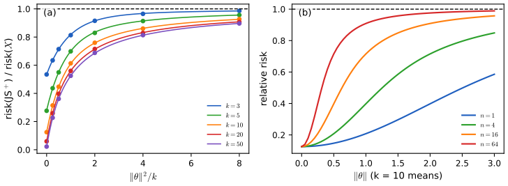
fig_12_s6. Download: PDF · SVGDemonstrations for this chapter
Each demonstration runs in the browser and links back to these notes. The ▶ Demo boxes above open them already set to the case under discussion.
| Demonstration | What you can see | Sections and results |
|---|---|---|
| Risk functions for a proportion | Exact risk functions of the MLE, the minimax estimator and any Beta-prior Bayes estimator, under squared or weighted loss; their maximum risks and their Bayes risks under a second "judge's" prior; both summaries against \(n\). Presets: 1 Example 12.5; 2 large \(n\); 3 small \(n\); 4 an informed judge; 5 the weighted loss of Example 12.13. | 12.2, 12.4; Filling the gaps 12.2, 12.3, 12.8 |
| Bayes estimators under three losses | A Beta posterior from binomial data with its mean, median, mode and the most probable window; the three posterior expected losses; the window action as the half-width shrinks; the exact Bayes risks of the three rules under the three losses. Presets: 1 a skewed posterior; 2 a narrow window; 3 a mode on the boundary; 4 a symmetric posterior; 5 a wide window. | 12.3; Theorems 12.7, 12.8; Filling the gap 12.5 |
| Stein's paradox | Exact and simulated risks of \(X\), James-Stein and its positive part against \(\|\th\|\); one simulated data set coordinate by coordinate; the relative risk against the dimension. Presets: 1 \(k=3\) at 0; 2 \(k=10\); 3 rotation invariance; 4 \(k=2\); 5 100 means. | 12.7; Theorem 12.D; Filling the gaps 12.17–12.19; Exercise 12.6 |
Related demonstrations: the Chapter 6 bias, variance and MSE demo (shrinkage of a single estimator), and in the companion courses the decision theory demo of Bayesian and Probabilistic Machine Learning, the Minkowski loss demo of Foundations of Deep Learning and the shrinkage paths demo of Statistical Learning: Theory and Methods. The Python code that produces every figure of this page is code/ch12_decision_theory.py (see the code index).
References
- Wasserman, L. (2004). All of Statistics: A Concise Course in Statistical Inference. Springer, New York. Chapter 12, pp. 193–205. www.stat.cmu.edu/~larry/all-of-statistics.
- Anderson, T. W. (1955). The integral of a symmetric unimodal function over a symmetric convex set and some probability inequalities. Proceedings of the American Mathematical Society, 6(2), 170–176.
- Berger, J. O. (1985). Statistical Decision Theory and Bayesian Analysis, 2nd edition. Springer, New York.
- Berliner, L. M. (1983). Improving on inadmissible estimators in the control problem. The Annals of Statistics, 11(3), 814–826.
- Blyth, C. R. (1951). On minimax statistical decision procedures and their admissibility. The Annals of Mathematical Statistics, 22(1), 22–42.
- Brown, L. D. (1971). Admissible estimators, recurrent diffusions, and insoluble boundary value problems. The Annals of Mathematical Statistics, 42(3), 855–903.
- Casella, G. and Berger, R. L. (2002). Statistical Inference, 2nd edition. Duxbury, Pacific Grove.
- Casella, G. and Strawderman, W. E. (1981). Estimating a bounded normal mean. The Annals of Statistics, 9(4), 870–878.
- Efron, B. and Morris, C. (1973). Stein's estimation rule and its competitors: an empirical Bayes approach. Journal of the American Statistical Association, 68(341), 117–130.
- Ferguson, T. S. (1967). Mathematical Statistics: A Decision Theoretic Approach. Academic Press, New York.
- Gill, R. D. and Levit, B. Y. (1995). Applications of the van Trees inequality: a Bayesian Cramér-Rao bound. Bernoulli, 1(1–2), 59–79.
- Hodges, J. L. and Lehmann, E. L. (1951). Some applications of the Cramér-Rao inequality. In Proceedings of the Second Berkeley Symposium on Mathematical Statistics and Probability, 13–22. University of California Press, Berkeley.
- James, W. and Stein, C. (1961). Estimation with quadratic loss. In Proceedings of the Fourth Berkeley Symposium on Mathematical Statistics and Probability, Vol. 1, 361–379. University of California Press, Berkeley.
- Le Cam, L. (1953). On some asymptotic properties of maximum likelihood estimates and related Bayes' estimates. University of California Publications in Statistics, 1, 277–330.
- Lehmann, E. L. and Casella, G. (1998). Theory of Point Estimation, 2nd edition. Springer, New York.
- Pinsker, M. S. (1980). Optimal filtering of square-integrable signals in Gaussian noise. Problems of Information Transmission, 16(2), 120–133.
- Stein, C. (1956). Inadmissibility of the usual estimator for the mean of a multivariate normal distribution. In Proceedings of the Third Berkeley Symposium on Mathematical Statistics and Probability, Vol. 1, 197–206. University of California Press, Berkeley.
- Stein, C. M. (1981). Estimation of the mean of a multivariate normal distribution. The Annals of Statistics, 9(6), 1135–1151.
- Van Trees, H. L. (1968). Detection, Estimation, and Modulation Theory, Part I. Wiley, New York.
The numerical statements in the text (the risk formulas and their summaries, the crossing at \(n=19.80\) and the width of the region where the minimax estimator wins, the posterior summaries and window actions, the exact Bayes risks of the three rules, the restricted Normal mean and its threshold \(m_0\), Hodges' risk and the van Trees bound, the many-means bounds, the James-Stein risks by series, by numerical integration and by simulation, the energies of Blyth's method, and the solutions of the exercises) were confirmed numerically.