Overview of Supervised Learning
Supervised learning predicts an output from inputs, using examples of both. This chapter sets out the whole subject in miniature. Two simple predictors mark the ends of a spectrum: the linear model fitted by least squares, rigid and stable, and the k-nearest-neighbour average, flexible and unstable. Decision theory says what they are both trying to estimate (the conditional mean, or the most probable class). The curse of dimensionality explains why the flexible end fails when there are many inputs, and why every practical method imposes structure: a penalty on roughness, a kernel that defines a neighbourhood, or a dictionary of basis functions. Each structure comes with a complexity parameter, and choosing it is a trade-off between bias and variance.
Ch. 1 Introduction Ch. 2 Supervised learning Ch. 3 Linear regression Ch. 4 Linear classification Ch. 5 Basis expansions Ch. 6 Kernel smoothing Ch. 7 Model assessment Ch. 8 Inference and averaging Ch. 9 Additive models and trees Ch. 10 Boosting Ch. 11 Neural networks Ch. 12 SVMs Ch. 13 Nearest neighbours Ch. 14 Unsupervised learning Ch. 15 Random forests Ch. 16 Ensembles Ch. 17 Graphical models Ch. 18 High-dimensional problems
How to read these notes
They follow the book. Sections carry the book's numbers (2.3, 2.3.1, ...) and every displayed equation that appears in the book carries the book's own number, e.g. \((2.13)\), so you can read these notes next to the book. Equations without a number are steps the book skips.
Filling the gaps. Where the book states a result without proof ("one can show", "it suffices", "Exercise 2.x"), an orange Filling the gap box or a proof gives the complete argument with its assumptions. Proofs start hidden: open one with its bar, or use the button below.
Figures and demonstrations. All eleven figures of the chapter are reproduced from scratch by the Python code, on the book's own simulated data where the book uses them. The ▶ Demo boxes open an interactive demonstration already set to the case being discussed.
Main reference
T. Hastie, R. Tibshirani and J. Friedman, The Elements of Statistical Learning: Data Mining, Inference, and Prediction, 2nd edition, Springer (2009), Chapter 2, pages 9–41 (book website, with the data sets: hastie.su.domains/ElemStatLearn). Section, equation, figure and exercise numbers below refer to this book.
The explanations, derivations, figures and code are my own; equations are cited by their numbers in the book.
Companion courses
Several topics of this chapter are treated, in a Bayesian or neural-network language, in the companion courses Bayesian and Probabilistic Machine Learning (Bishop 2006) and Foundations of Deep Learning (Bishop and Bishop 2024). Where a full proof is given there, these notes give the statement, a short argument and a link.
- Section 2.3.1 (least squares, the normal equations): Deep Learning, Section 4.1.3 (Result 4.2); Machine Learning, Section 3.1.1. Least squares for classification: Deep Learning, Section 5.1.4.
- Section 2.3.2 (nearest neighbours): Machine Learning, Section 2.5.2, with the Cover-Hart bound in Result 2.28.
- Section 2.4 (decision theory): Machine Learning, Section 1.5 (Result 1.15, 1.18, 1.19); Deep Learning, Section 4.2 and Section 5.2.
- Section 2.5 (the curse of dimensionality): Machine Learning, Section 1.4; Deep Learning, Sections 6.1.1 and 6.1.2.
- Section 2.6.3 (likelihood, cross-entropy): Machine Learning, Result 1.9; Deep Learning, Section 6.4. Section 2.8.1 (penalty as prior): Machine Learning, Result 1.10. Section 2.8.2 (Nadaraya-Watson): Machine Learning, Section 6.3.1. Section 2.8.3 (neural networks as adaptive bases): Deep Learning, Section 6.2.2.
- Section 2.9 (the bias-variance trade-off): Deep Learning, Section 4.3; Machine Learning, Section 3.2 with its bias-variance demo.
New here: the effective number of parameters \(N/k\) of nearest neighbours and the exact optimism of its training error, a proof that \(k\)-NN is consistent, the best linear predictor as a projection, exact formulas for the bias and variance behind Figures 2.7 and 2.8, the exact finite-sample version of (2.28) for Gaussian inputs, and a computed Figure 2.11.
The chapter at a glance
- 2.3 Least squares fits a global linear function (Result 2.1); \(k\)-NN averages locally and has about \(N/k\) effective parameters (Result 2.2). On the book's mixture data they bracket the Bayes rate (Figure 2.4).
- 2.4 Under squared loss the best predictor is the regression function \(\E(Y\given X=x)\) (Result 2.3), which \(k\)-NN estimates consistently (Result 2.4) and least squares approximates by its best linear projection (Result 2.5); absolute loss gives the median (Result 2.6), 0-1 loss the Bayes classifier (Result 2.7).
- 2.5 In \(p\) dimensions a neighbourhood holding a fraction \(r\) of the data has edge \(r^{1/p}\), and the nearest of \(N\) points is far away (Results 2.9, 2.10); least squares escapes because it assumes linearity, with error \(\sigma^2(1+p/N)\) (Result 2.11).
- 2.6–2.8 Additive-error models, least squares as maximum likelihood (Result 2.13); without restrictions the fitting problem has infinitely many solutions (Result 2.14); penalties, kernels and basis expansions are the three ways of restricting it (Results 2.15–2.17).
- 2.9 For \(k\)-NN the expected prediction error is noise plus squared bias plus \(\sigma^2/k\) (Result 2.18); training error always falls with complexity, test error is U-shaped (Figure 2.11).
Notation. Inputs \(X\in\R^p\) (a random vector) with observed values \(x_i\); quantitative output \(Y\), qualitative output \(G\) taking values in a set \(\cG\) of \(K\) classes. Training data \(\cT=\{(x_i,y_i)\}_{i=1}^N\); \(\bX\) is the \(N\times p\) matrix with rows \(x_i^\T\) (with a first column of ones when an intercept is included) and \(\by=(y_1,\dots,y_N)^\T\). Vectors are columns. \(\Ind(\cdot)\) is the indicator function.
Prerequisites. Conditional expectation, the multivariate normal distribution, and the linear algebra of least squares (the matrix calculus and singular value decomposition sections of the companion course's toolkit).
2.1 Introduction
p. 9 In each of the motivating problems of Chapter 1 some variables, the inputs, are measured or set, and they influence one or more outputs; the task is to predict the outputs from the inputs. Because the training data contain the correct output for each input, as if a teacher had supplied it, this is called supervised learning. Statisticians say predictors or independent variables for the inputs and responses or dependent variables for the outputs; pattern recognition says features.
2.2 Variable Types and Terminology
pp. 9–11 Outputs are quantitative (a measurement, where closeness of values means closeness in nature) or qualitative (a label from a finite set \(\cG\), such as the three Iris species or the ten digits, with no natural order). Predicting a quantitative output is regression; predicting a qualitative one is classification. Both are function approximation. A third type is ordered categorical (small, medium, large): ordered, but without a metric.
Definition 2.1 (coding a qualitative variable) p. 10
A two-level variable is coded by one bit, 0/1 or \(-1/1\); such numeric codes are called targets. A \(K\)-level variable \(G\) is coded by dummy variables: the vector \(Y=(Y_1,\dots,Y_K)\) with \(Y_k=\Ind(G=\mathcal{G}_k)\), exactly one of which equals 1. This coding is symmetric in the levels, unlike, say, the codes \(1,\dots,K\), which would impose an order and equal spacings.
Generic variables are written in capitals (\(X\), \(Y\), \(G\)), observed values in lower case (\(x_i\)); a \(p\)-vector of inputs for observation \(i\) is \(x_i\), while the bold \(\mathbf{x}_j\) is the \(N\)-vector of all observations on variable \(X_j\). The learning task: given \(X\), produce a prediction \(\hat Y\) in the same space as \(Y\) (or \(\hat G\in\cG\)). For two classes one can code \(G\) as \(Y\in\{0,1\}\), predict \(\hat Y\) as a quantitative output, and set \(\hat G\) by whether \(\hat y>0.5\).
2.3 Two Simple Approaches to Prediction: Least Squares and Nearest Neighbors
p. 11 The linear model makes strong assumptions about structure and gives stable but possibly inaccurate predictions; \(k\)-nearest neighbours assumes very little and gives predictions that are often accurate but unstable. Most methods in the book sit between the two.
2.3.1 Linear Models and Least Squares
pp. 11–14 Given \(X^\T=(X_1,\dots,X_p)\), the linear model predicts
\[ \hat Y=\hat\beta_0+\sum_{j=1}^pX_j\hat\beta_j , \tag{2.1} \]or, with the constant 1 included in \(X\) and \(\hat\beta_0\) in \(\hat\beta\),
\[ \hat Y=X^\T\hat\beta . \tag{2.2} \]The intercept \(\hat\beta_0\) is called the bias in machine learning. In the \((p+1)\)-dimensional input-output space the graph \(\{(X,\hat Y)\}\) is a hyperplane; as a function of the inputs, \(f(X)=X^\T\beta\) has constant gradient (the slope coefficients), pointing in the direction of steepest increase. From here on the intercept is included in \(\beta\), so \(\bX\) has a first column of ones (and \(p+1\) columns, although the book keeps writing \(N\times p\)). The least-squares fit minimises the residual sum of squares
\[ \RSS(\beta)=\sum_{i=1}^N(y_i-x_i^\T\beta)^2 , \tag{2.3} \] \[ \RSS(\beta)=(\by-\bX\beta)^\T(\by-\bX\beta). \tag{2.4} \]Result 2.1 (the normal equations) p. 12, (2.3)–(2.6)
The minimisers of (2.4) are exactly the solutions of the normal equations
\[ \bX^\T(\by-\bX\beta)=0 . \tag{2.5} \]A solution always exists. If \(\bX^\T\bX\) is nonsingular (equivalently, \(\bX\) has full column rank) it is unique,
\[ \hat\beta=(\bX^\T\bX)^{-1}\bX^\T\by , \tag{2.6} \]and in all cases the fitted vector \(\hat\by=\bX\hat\beta\) is the same for every minimiser: the orthogonal projection of \(\by\) onto the column space of \(\bX\).
Proof (short; the full argument is in the companion course)
Expanding, \(\RSS(\beta)=\by^\T\by-2\beta^\T\bX^\T\by+\beta^\T\bX^\T\bX\beta\), whose gradient is \(-2\bX^\T(\by-\bX\beta)\): zero exactly at (2.5). For a solution \(\hat\beta\) of (2.5) and any \(v\), the identity
\[ \RSS(\hat\beta+v)=\RSS(\hat\beta)-2v^\T\bX^\T(\by-\bX\hat\beta)+\|\bX v\|^2=\RSS(\hat\beta)+\|\bX v\|^2 \]shows that \(\hat\beta\) is a global minimiser and that \(\hat\beta+v\) is another one if and only if \(\bX v=0\), which leaves the fitted vector unchanged. When \(\bX^\T\bX\) is invertible, (2.5) has the single solution (2.6). Existence in general (via the pseudo-inverse) and the projection property are proved in Deep Learning, Results 4.2, 4.3 and 4.5. ∎
The fitted value at \(x_i\) is \(\hat y_i=x_i^\T\hat\beta\) and at a new input \(x_0\) it is \(x_0^\T\hat\beta\): the whole fitted surface is described by \(p+1\) numbers, which suggests that a modest data set suffices to fit it.
A classification example. Figure 2.1 shows 200 points in the plane, 100 in class BLUE and 100 in class ORANGE, simulated from a model described in Section 2.3.3. Code \(Y=0\) for BLUE and \(Y=1\) for ORANGE, fit (2.6), and convert the fitted value into a class by
\[ \hat G=\begin{cases}\text{ORANGE} & \text{if } \hat Y>0.5,\\ \text{BLUE} & \text{if } \hat Y\le0.5.\end{cases} \tag{2.7} \]The ORANGE region is \(\{x:x^\T\hat\beta>0.5\}\) and the decision boundary \(\{x:x^\T\hat\beta=0.5\}\) is a straight line.
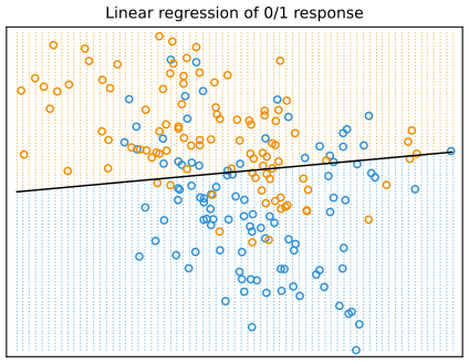
fig_2_1. Reproduces Hastie, Tibshirani and Friedman (2009), Figure 2.1. Download: PDF · SVGFilling the gap 2.1: the numbers behind Figure 2.1 p. 13
The fitted line and its errors
On the book's data (the file ESL.mixture.rda from the book's website) the least-squares coefficients are
so the boundary \(\hat\beta_0+\hat\beta_1x_1+\hat\beta_2x_2=0.5\) is the line \(x_2=0.6849+0.0907\,x_1\): almost horizontal, because the class means differ mainly in \(x_2\) (the BLUE cluster centres were drawn around \((1,0)\), the ORANGE ones around \((0,1)\)). The rule (2.7) misclassifies 54 of the 200 training points (27.0%), and 28.75% of an independent test set of 10,000 points (Figure 2.4). The fitted values are not probabilities: on the training inputs they range from \(-0.23\) to \(1.05\) (see Result 2.8).
Two scenarios would explain the errors: (1) each class is a bivariate Gaussian with uncorrelated components and different means, in which case a linear boundary is the best possible (Chapter 4) and the overlap cannot be avoided; or (2) each class is a mixture of 10 low-variance Gaussians whose means are themselves Gaussian, in which case the optimal boundary is nonlinear, even disconnected. A mixture is easiest to describe generatively: first draw which component to use, then draw from it.
See also (companion courses): Deep Learning, Section 4.1.3 (maximum likelihood and least squares) and Section 5.1.4 (least squares for classification, and why it is not robust).
2.3.2 Nearest-Neighbor Methods
pp. 14–16 The \(k\)-nearest-neighbour fit averages the responses of the \(k\) training points closest to \(x\):
\[ \hat Y(x)=\frac1k\sum_{x_i\in N_k(x)}y_i , \tag{2.8} \]where \(N_k(x)\) is the set of the \(k\) closest \(x_i\) in Euclidean distance. With the 0/1 coding, \(\hat Y\) is the proportion of ORANGE among the neighbours, and (2.7) becomes a majority vote. Figure 2.2 uses \(k=15\); Figure 2.3 uses \(k=1\), where each point \(x_i\) owns the tile of the plane closer to it than to any other training point (the Voronoi tessellation), and \(\hat G\) equals \(g_i\) on that tile.
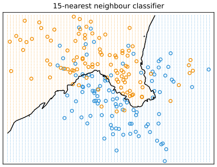
fig_2_2. Reproduces Hastie, Tibshirani and Friedman (2009), Figure 2.2. Download: PDF · SVG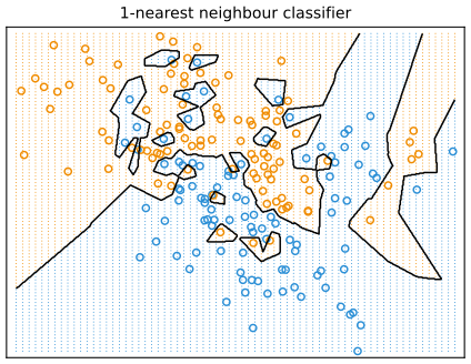
fig_2_3. Reproduces Hastie, Tibshirani and Friedman (2009), Figure 2.3. Download: PDF · SVGThe book makes two claims here that deserve proof: that the training error should be roughly increasing in \(k\) and zero at \(k=1\), and that the effective number of parameters of \(k\)-NN is \(N/k\) (larger than the \(p+1\) of least squares, and decreasing in \(k\)). The heuristic is that \(N/k\) non-overlapping neighbourhoods would each fit one mean. The following makes it exact for regression.
Result 2.2 (\(k\)-NN is a linear smoother with \(N/k\) degrees of freedom) p. 15
Let the inputs \(x_1,\dots,x_N\) be distinct and fixed, with no ties among the distances that define the neighbourhoods, and let \(y_i=f(x_i)+\varepsilon_i\) with independent errors of mean 0 and variance \(\sigma^2\). The vector of fitted values is \(\hat\by=\bS\by\), with
\[ \bS_{ij}=\tfrac1k\,\Ind\big(x_j\in N_k(x_i)\big),\qquad \bS_{ii}=\tfrac1k,\qquad \Tr\bS=\frac Nk . \]For any linear smoother \(\hat\by=\bS\by\), let \(\by'=f+\varepsilon'\) be new responses at the same inputs. Then
\[ \E\,\tfrac1N\|\by'-\hat\by\|^2-\E\,\tfrac1N\|\by-\hat\by\|^2=\frac{2\sigma^2}{N}\Tr\bS , \]which for \(k\)-NN is \(2\sigma^2/k\). So \(\Tr\bS=N/k\) plays the role that the number of parameters \(p+1\) plays for least squares, where \(\bS\) is the hat matrix and \(\Tr\bS=p+1\).
Proof
(2.8) at \(x_i\) is a fixed linear combination of the \(y_j\), with weight \(1/k\) on each of the \(k\) neighbours: that is the row \(i\) of \(\bS\). Because the inputs are distinct, \(x_i\) is at distance 0 from itself and strictly further from every other point, so it is its own first neighbour and \(\bS_{ii}=1/k\); summing the diagonal gives \(N/k\).
For a general linear smoother write \(f=(f(x_1),\dots,f(x_N))^\T\). Then \(\by-\bS\by=(\bI-\bS)f+(\bI-\bS)\varepsilon\), and since \(\E\varepsilon=0\), \(\E\varepsilon\varepsilon^\T=\sigma^2\bI\),
\[ \E\|\by-\bS\by\|^2=\|(\bI-\bS)f\|^2+\sigma^2\Tr\big((\bI-\bS)^\T(\bI-\bS)\big)=\|(\bI-\bS)f\|^2+\sigma^2\big(N-2\Tr\bS+\Tr\bS^\T\bS\big). \]For the new responses, \(\by'-\bS\by=(\bI-\bS)f+\varepsilon'-\bS\varepsilon\) with \(\varepsilon'\) independent of \(\varepsilon\), so
\[ \E\|\by'-\bS\by\|^2=\|(\bI-\bS)f\|^2+\sigma^2N+\sigma^2\Tr\bS^\T\bS . \]The difference is \(2\sigma^2\Tr\bS\); divide by \(N\). For \(k\)-NN, row \(i\) of \(\bS\) has \(k\) entries \(1/k\), so \(\Tr\bS^\T\bS=\sum_{ij}\bS_{ij}^2=N/k\), and the expected training error of point \(i\) works out to \(b_i^2+\sigma^2(1-1/k)\), its expected test error to \(\sigma^2+b_i^2+\sigma^2/k\), where \(b_i\) is the \(i\)th entry of \((\bI-\bS)f\). For least squares \(\bS=\bX(\bX^\T\bX)^{-1}\bX^\T\) and \(\Tr\bS=\Tr\big((\bX^\T\bX)^{-1}\bX^\T\bX\big)=p+1\). ∎
Chapter 7 takes this as the definition of the effective number of parameters, \(\mathrm{df}=\sum_i\Cov(\hat y_i,y_i)/\sigma^2\), which equals \(\Tr\bS\) for any linear smoother. It also explains why training error cannot choose \(k\): it is optimistic by \(2\sigma^2/k\), most of all at \(k=1\).
Filling the gap 2.2: the training error of \(k\)-NN is zero at \(k=1\), but not monotone p. 15
Details
With distinct inputs, a training point is its own nearest neighbour, so the 1-NN rule reproduces its label: the training error is exactly 0 (with repeated inputs carrying different labels it need not be). For larger \(k\) the book says the training error is "approximately" increasing. It is not exactly so: on the mixture data the training error for \(k=9,11,13,15\) is \(15.5\%,18.5\%,16.0\%,15.5\%\). A majority vote changes only when the added neighbour flips the majority, and flips can go either way. In expectation, for regression with a fixed design, Result 2.2 shows the training error is \(\overline{b^2}(k)+\sigma^2(1-1/k)\), the sum of an average squared bias that typically grows with \(k\) and a term that grows with \(k\); this is what makes the trend increasing.
For Gaussian classes (Scenario 1) \(k\)-NN boundaries would be needlessly noisy; for the clustered mixture (Scenario 2) they seem more appropriate.
See also (companion course): Machine Learning, Section 2.5.2 (nearest-neighbour density estimation and classification) and Result 2.28 (the asymptotic error of 1-NN is at most twice the Bayes rate).
2.3.3 From Least Squares to Nearest Neighbors
pp. 16–18 The least-squares boundary is smooth and stable but relies on linearity being appropriate: in the language of Section 2.9, low variance and possibly high bias. A \(k\)-NN boundary adapts to anything, but each piece of it depends on a handful of points: high variance, low bias. The data were in fact generated by a model between the two scenarios, closer to the second.
Definition 2.2 (the mixture model of Figures 2.1–2.5) pp. 16–17
Draw ten means \(m_1,\dots,m_{10}\) from \(\N\big((1,0)^\T,\bI\big)\) for BLUE and ten from \(\N\big((0,1)^\T,\bI\big)\) for ORANGE, and keep them fixed. For each observation of a class, pick one of its ten means with probability \(1/10\) and draw \(X\sim\N(m_k,\bI/5)\). So the class densities are
\[ f_{\rm B}(x)=\frac1{10}\sum_{k\in\rm B}\phi(x;m_k,\bI/5),\qquad f_{\rm O}(x)=\frac1{10}\sum_{k\in\rm O}\phi(x;m_k,\bI/5), \]with \(\phi(x;m,\bI/5)=\frac{5}{2\pi}\exp\big(-\tfrac52\|x-m\|^2\big)\). The training set has 100 points from each class.
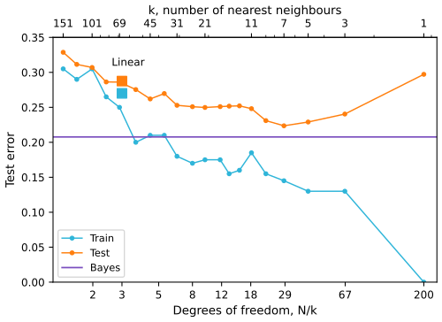
fig_2_4. Reproduces Hastie, Tibshirani and Friedman (2009), Figure 2.4. Download: PDF · SVGFilling the gap 2.3: how Figure 2.4 is computed, and its numbers p. 17
Details
The training data are the book's 200 points, so the training curve is the book's exactly. The test set is not distributed with the book; here it is simulated from Definition 2.2 with the book's own 20 means (5,000 points per class). The Bayes rate is not simulated: it is the integral \(\tfrac12\int\min\{f_{\rm B}(x),f_{\rm O}(x)\}\,\d x\) (Result 2.7), computed on a grid of step 0.01, which gives \(0.2076\). The results:
| rule | training error | test error |
|---|---|---|
| least squares (3 parameters) | 0.270 | 0.2875 |
| 1-NN | 0 | 0.2972 |
| 15-NN | 0.155 | 0.2517 |
| 7-NN (smallest test error) | 0.145 | 0.2236 |
| 151-NN | 0.305 | 0.3287 |
| Bayes rule (knows the means) | 0.2110 |
The Bayes rule's error on this particular test set, 0.2110, differs from the Bayes rate 0.2076 by sampling error (standard error about 0.004). No rule, however flexible, can beat the Bayes rate on average.
Many popular methods are refinements of these two: kernel methods weight neighbours smoothly by distance instead of the 0/1 weights of \(k\)-NN; in high dimensions the distance is modified to emphasise some variables; local regression fits linear models by locally weighted least squares instead of local constants; basis expansions make linear models arbitrarily flexible; and projection pursuit and neural networks are sums of nonlinearly transformed linear models.
2.4 Statistical Decision Theory
pp. 18–22 Let \(X\in\R^p\) and \(Y\in\R\) be random with joint distribution \(\Pr(X,Y)\). A predictor \(f(X)\) is judged by a loss \(L(Y,f(X))\), most often squared error, which gives the expected (squared) prediction error
\[ \EPE(f)=\E\big(Y-f(X)\big)^2 \tag{2.9} \] \[ =\int[y-f(x)]^2\Pr(\d x,\d y). \tag{2.10} \]Conditioning on \(X\) (that is, factoring \(\Pr(X,Y)=\Pr(Y\given X)\Pr(X)\) and integrating in two steps),
\[ \EPE(f)=\E_X\E_{Y|X}\big([Y-f(X)]^2\given X\big) \tag{2.11} \]and it suffices to minimise pointwise:
\[ f(x)=\argmin_c\E_{Y|X}\big([Y-c]^2\given X=x\big). \tag{2.12} \]The solution is the conditional expectation, the regression function,
\[ f(x)=\E(Y\given X=x). \tag{2.13} \]Result 2.3 (the regression function minimises the expected squared error) p. 18, (2.9)–(2.13)
Assume \(\E Y^2\lt\infty\) and write \(m(x)=\E(Y\given X=x)\). For every function \(f\) with \(\E f(X)^2\lt\infty\),
\[ \EPE(f)=\E\big(Y-m(X)\big)^2+\E\big(m(X)-f(X)\big)^2 . \]Hence \(m\) minimises EPE, the minimum is \(\E\Var(Y\given X)\), and any other minimiser equals \(m\) except on a set of \(X\)-probability zero.
Proof, and why "pointwise" is legitimate
Write \(Y-f(X)=\big(Y-m(X)\big)+\big(m(X)-f(X)\big)\) and expand the square. The cross term is
\[ 2\,\E\Big[\big(m(X)-f(X)\big)\big(Y-m(X)\big)\Big]=2\,\E\Big[\big(m(X)-f(X)\big)\,\E\big(Y-m(X)\given X\big)\Big]=0, \]by the tower property (a function of \(X\) can be taken out of the inner conditional expectation) and \(\E(Y\given X)=m(X)\); it is finite by the Cauchy-Schwarz inequality, since \(\E m(X)^2\le\E Y^2\). The remaining two terms are the claim. The second is nonnegative and vanishes iff \(f(X)=m(X)\) almost surely.
The pointwise view (2.12) says the same thing for each \(x\): \[ g(x,c)=\E[(Y-c)^2\given X=x]=\Var(Y\given X=x)+(c-m(x))^2 \] is minimised at \(c=m(x)\). Since \(\EPE(f)=\E\,g(X,f(X))\) and \(g(x,f(x))\ge g(x,m(x))\) for every \(x\), integrating the inequality gives \(\EPE(f)\ge\EPE(m)\). Choosing \(f(x)\) separately for each \(x\) is allowed because no constraint links the values of \(f\) at different points. ∎
See also (companion courses): Machine Learning, Result 1.18 (the same result by the calculus of variations) and Deep Learning, Result 4.9.
Nearest neighbours as a direct estimate. Ideally we would average all \(y_i\) with \(x_i=x\); since there is usually at most one, \(k\)-NN settles for
\[ \hat f(x)=\Ave\big(y_i\given x_i\in N_k(x)\big), \tag{2.14} \]which makes two approximations: an expectation is replaced by a sample average, and conditioning at a point by conditioning on a neighbourhood. The book states that under mild conditions, as \(N,k\to\infty\) with \(k/N\to0\), \(\hat f(x)\to\E(Y\given X=x)\). Here is a proof.
Result 2.4 (consistency of \(k\)-NN regression at a point) p. 19
Let \((X_i,Y_i)\) be independent copies of \((X,Y)\). Fix \(x_0\) in the support of \(X\) (every ball around \(x_0\) has positive probability), assume \(m(x)=\E(Y\given X=x)\) is continuous at \(x_0\) and \(\Var(Y\given X=x)\le s^2\) for all \(x\). If \(k=k_N\to\infty\) and \(k_N/N\to0\), then \(\hat f(x_0)\to m(x_0)\) in probability.
Proof
Condition on the inputs \(X_1,\dots,X_N\); they determine the neighbours \(X_{(1)},\dots,X_{(k)}\) of \(x_0\) (ties broken by any fixed rule). Given the inputs, the \(Y_i\) are independent with means \(m(X_i)\) and variances at most \(s^2\). Split
\[ \hat f(x_0)-m(x_0)=\underbrace{\frac1k\sum_{l=1}^k\big(m(X_{(l)})-m(x_0)\big)}_{B}+\underbrace{\frac1k\sum_{l=1}^k\big(Y_{(l)}-m(X_{(l)})\big)}_{V}. \]Variance. Given the inputs, \(V\) has mean 0 and variance at most \(s^2/k\), so \(\E V^2\le s^2/k\to0\) and \(V\to0\) in probability (Chebyshev).
Bias. Fix \(\epsilon>0\). By continuity there is \(\delta>0\) with \(|m(x)-m(x_0)|\lt\epsilon\) whenever \(\|x-x_0\|\lt\delta\). Let \(q=\Pr(\|X-x_0\|\lt\delta)>0\) and let \(M_N\sim\mathrm{Bin}(N,q)\) count the inputs in that ball. On the event \(M_N\ge k\) all \(k\) neighbours lie in the ball, so \(|B|\lt\epsilon\). Since \(k/N\to0\lt q\), for large \(N\) we have \(Nq-k>0\) and, by Chebyshev,
\[ \Pr(M_N\lt k)\le\Pr\big(|M_N-Nq|\ge Nq-k\big)\le\frac{Nq(1-q)}{(Nq-k)^2}\to0 . \]So \(\Pr(|B|\ge\epsilon)\to0\). Combining, \[ \Pr(|\hat f(x_0)-m(x_0)|\ge2\epsilon)\le\Pr(|B|\ge\epsilon)+\Pr(|V|\ge\epsilon)\to0. \] ∎
The proof shows where the rate comes from: the variance is \(O(1/k)\), while the bias is controlled by the radius of the neighbourhood holding \(k\) points, which for a smooth density behaves like \((k/N)^{1/p}\). For fixed accuracy that radius shrinks ever more slowly as \(p\) grows: the convergence still holds, but its rate deteriorates with dimension (Section 2.5). Stone (1977) proved much stronger, distribution-free versions.
Least squares as a model-based approach. Linear regression assumes instead that the regression function is approximately linear,
\[ f(x)\approx x^\T\beta . \tag{2.15} \]Substituting into (2.9) and differentiating gives
\[ \beta=[\E(XX^\T)]^{-1}\E(XY). \tag{2.16} \]Result 2.5 (the best linear predictor) p. 19, (2.15)–(2.16)
Assume \(\E\|X\|^2\lt\infty\), \(\E Y^2\lt\infty\) and \(\E(XX^\T)\) invertible. Then (2.16) is the unique minimiser of \(\E(Y-X^\T\beta)^2\). It is also the unique minimiser of \(\E\big(m(X)-X^\T\beta\big)^2\): \(X^\T\beta\) is the projection of the regression function onto the linear functions, whether or not \(m\) is linear. The least-squares estimate (2.6) is its sample version and converges to it almost surely as \(N\to\infty\).
Proof
\[ \E(Y-X^\T\beta)^2=\E Y^2-2\beta^\T\E(XY)+\beta^\T\E(XX^\T)\beta \] is a quadratic in \(\beta\) with gradient \(-2\E(XY)+2\E(XX^\T)\beta\) and Hessian \(2\E(XX^\T)\), positive definite because \(v^\T\E(XX^\T)v=\E(X^\T v)^2\gt0\) for \(v\ne0\) when the matrix is invertible. So the unique stationary point (2.16) is the minimiser. By the tower property \(\E(XY)=\E\big(X\,\E(Y\given X)\big)=\E\big(X m(X)\big)\), so replacing \(Y\) by \(m(X)\) changes neither the gradient nor the solution. Finally \(\hat\beta=\big(\tfrac1N\bX^\T\bX\big)^{-1}\tfrac1N\bX^\T\by\), and by the strong law of large numbers \(\tfrac1N\sum_ix_ix_i^\T\to\E(XX^\T)\) and \(\tfrac1N\sum_ix_iy_i\to\E(XY)\) almost surely; matrix inversion is continuous at an invertible matrix. ∎
So both methods approximate conditional expectations by averages, under different assumptions: least squares that \(f\) is well approximated by a globally linear function, \(k\)-NN that it is well approximated by a locally constant one. Note that (2.16) does not condition on \(X\): knowledge of the functional form lets it pool over all values of \(X\). Between the two are model-based methods such as additive models,
\[ f(X)=\sum_{j=1}^pf_j(X_j), \tag{2.17} \]which keep additivity but leave each \(f_j\) arbitrary; fitting them uses one-dimensional smoothers (for example \(k\)-NN) for each coordinate in turn (Chapter 9), and so escapes high-dimensional conditioning by assuming additivity.
Other losses. With absolute error \(\E|Y-f(X)|\) the solution is the conditional median,
\[ \hat f(x)=\median(Y\given X=x), \tag{2.18} \]a different measure of location whose estimates are more robust to outliers; the derivative of the absolute loss is discontinuous at zero, which long made it less popular.
Result 2.6 (absolute loss gives the conditional median) p. 20, (2.18)
Let \(F\) be the distribution function of a random variable \(Y\) with \(\E|Y|\lt\infty\), and \(g(c)=\E|Y-c|\). Then \(g\) is convex, and \(c\) minimises \(g\) if and only if \(F(c^-)\le\tfrac12\le F(c)\), that is, \(c\) is a median. Applied to the conditional distribution of \(Y\) given \(X=x\), and pointwise as in Result 2.3, this gives (2.18).
Proof
For \(c\lt c'\), a case check gives \(|y-c'|-|y-c|=c'-c\) if \(y\le c\), \(=-(c'-c)\) if \(y\ge c'\), and \(=c+c'-2y\in(-(c'-c),c'-c)\) if \(c\lt y\lt c'\). Taking expectations,
\[ g(c')-g(c)=(c'-c)\big[F(c)-\Pr(Y\ge c')\big]+\E\big[(c+c'-2Y)\Ind(c\lt Y\lt c')\big], \]and the last term is at most \((c'-c)\Pr(c\lt Y\lt c')\) in absolute value. Dividing by \(c'-c\) and letting \(c'\downarrow c\) (the probability \(\Pr(c\lt Y\lt c')\to0\)) gives the right derivative \(g'_+(c)=F(c)-(1-F(c))=2F(c)-1\); similarly the left derivative is \(g'_-(c)=2F(c^-)-1\). Both are nondecreasing in \(c\), so \(g\) is convex, and a convex function is minimised exactly where \(g'_-(c)\le0\le g'_+(c)\), i.e. \(F(c^-)\le\tfrac12\le F(c)\). ∎
See also (companion courses): Deep Learning, Result 4.10 and Machine Learning, Result 1.19 (the Minkowski loss).
Categorical outputs. For \(G\in\cG=\{\mathcal{G}_1,\dots,\mathcal{G}_K\}\) the loss is a \(K\times K\) matrix \(\mathbf{L}\), zero on the diagonal and nonnegative elsewhere, with \(L(k,\ell)\) the price of classifying an observation of class \(\mathcal{G}_k\) as \(\mathcal{G}_\ell\). The zero-one loss charges 1 for every mistake. Then
\[ \EPE=\E[L(G,\hat G(X))], \tag{2.19} \] \[ \EPE=\E_X\sum_{k=1}^KL[\mathcal{G}_k,\hat G(X)]\Pr(\mathcal{G}_k\given X), \tag{2.20} \] \[ \hat G(x)=\argmin_{g\in\cG}\sum_{k=1}^KL(\mathcal{G}_k,g)\Pr(\mathcal{G}_k\given X=x). \tag{2.21} \]With the zero-one loss this simplifies to
\[ \hat G(x)=\argmin_{g\in\cG}\big[1-\Pr(g\given X=x)\big] \tag{2.22} \]or simply
\[ \hat G(X)=\mathcal{G}_k\ \text{ if }\ \Pr(\mathcal{G}_k\given X=x)=\max_{g\in\cG}\Pr(g\given X=x). \tag{2.23} \]Result 2.7 (the Bayes classifier and the Bayes rate) pp. 20–21, (2.19)–(2.23)
(a) For any loss matrix, the rule (2.21) minimises (2.19) over all classifiers. (b) For the zero-one loss it is the rule (2.23), the Bayes classifier, and its error, the Bayes rate, is \(1-\E\big[\max_k\Pr(\mathcal{G}_k\given X)\big]\). (c) With two classes of prior probabilities \(\pi_0,\pi_1\) and densities \(f_0,f_1\), the Bayes rate is \(\int\min\{\pi_0f_0(x),\pi_1f_1(x)\}\,\d x\).
Proof
(a) Conditioning on \(X\), \[ \E[L(G,\hat G(X))\given X=x]=\sum_kL(\mathcal{G}_k,\hat G(x))\Pr(\mathcal{G}_k\given X=x), \] which gives (2.20). For each \(x\) this is a function \(h(x,g)\) of the chosen class \(g=\hat G(x)\) only, and (2.21) picks the \(g\) with the smallest value; so \(h(x,\hat G(x))\ge h(x,\hat G_{\rm Bayes}(x))\) for any rule and every \(x\), and taking \(\E_X\) gives the claim (exactly as in Result 2.3). (b) With \(L(k,\ell)=1-\Ind(k=\ell)\), \(h(x,g)=\sum_{k:\mathcal{G}_k\ne g}\Pr(\mathcal{G}_k\given x)=1-\Pr(g\given x)\), which is (2.22), minimised by the most probable class (2.23); its conditional error is \(1-\max_k\Pr(\mathcal{G}_k\given x)\), and averaging over \(X\) gives the Bayes rate. (c) With two classes, \(1-\max\) of two probabilities summing to 1 is their minimum, and by Bayes' theorem \(\Pr(k\given x)=\pi_kf_k(x)/f(x)\) with \(f=\pi_0f_0+\pi_1f_1\) the density of \(X\). So the Bayes rate is \[ \int\min_k\{\pi_kf_k(x)/f(x)\}f(x)\,\d x=\int\min\{\pi_0f_0,\pi_1f_1\}\,\d x. \] ∎
See also (companion courses): Machine Learning, Result 1.15 and Deep Learning, Results 5.5 and 5.6 (minimum misclassification and minimum expected loss).
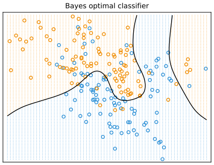
fig_2_5. Reproduces Hastie, Tibshirani and Friedman (2009), Figure 2.5. Download: PDF · SVGFilling the gap 2.4: the Bayes boundary of the mixture data (Exercise 2.2) p. 21
Derivation
The classes have equal priors \(\tfrac12\), so by Result 2.7 the Bayes rule chooses ORANGE iff \(f_{\rm O}(x)\gt f_{\rm B}(x)\). The common factors \(\frac1{10}\cdot\frac5{2\pi}\) cancel, and the boundary is
\[ \Big\{x:\ \sum_{k\in\rm O}\exp\big(-\tfrac52\|x-m_k\|^2\big)=\sum_{k\in\rm B}\exp\big(-\tfrac52\|x-m_k\|^2\big)\Big\}, \]the 0.5 contour of \(\Pr(\text{ORANGE}\given x)=f_{\rm O}/(f_{\rm O}+f_{\rm B})\). It has no closed form; it is drawn as the contour of this function on a fine grid. The probabilities recomputed this way agree with the values stored in the book's data file to \(10^{-14}\). The Bayes rate is \(\tfrac12\int\min(f_{\rm B},f_{\rm O})=0.2076\).
\(k\)-NN approximates the Bayes classifier directly: a majority vote in a neighbourhood estimates \(\Pr(\mathcal{G}_k\given X=x)\) by a proportion in a region around \(x\). The dummy-variable approach does too:
Result 2.8 (regression on dummy variables estimates the posterior) p. 22
With the dummy coding of Definition 2.1, \(\E(Y_k\given X)=\Pr(G=\mathcal{G}_k\given X)\), so classifying to the largest fitted value is a plug-in version of the Bayes classifier. If the \(K\) responses are fitted by least squares with an intercept, the fitted values sum to 1 at every \(x\), but they can be negative or exceed 1.
Proof
\(Y_k\) is the indicator of \(\{G=\mathcal{G}_k\}\), and the conditional expectation of an indicator is the conditional probability of the event. For the second statement collect the responses in the \(N\times K\) indicator matrix \(\mathbf{Y}\), whose rows sum to 1: \(\mathbf{Y}\one_K=\one_N\). With the intercept the first column of \(\bX\) is \(\one_N=\bX e_1\), so the coefficient matrix \(\hat{\mathbf{B}}=(\bX^\T\bX)^{-1}\bX^\T\mathbf{Y}\) satisfies \(\hat{\mathbf{B}}\one_K=(\bX^\T\bX)^{-1}\bX^\T\bX e_1=e_1\), and at any input \(x\) (with its leading 1) the fitted values sum to \(x^\T\hat{\mathbf{B}}\one_K=x^\T e_1=1\). Nothing keeps each one in \([0,1]\): in Figure 2.1 the fitted value \(x^\T\hat\beta\) ranges over \([-0.27,1.11]\) on the plotting grid. ∎
See also (companion course): Deep Learning, Result 5.3 (the regression function of a 1-of-K target is the posterior).
2.5 Local Methods in High Dimensions
pp. 22–27 It seems that with enough data \(k\)-NN averaging could always approximate the regression function. In high dimensions this intuition fails: the curse of dimensionality (Bellman 1961). Three manifestations follow.
Result 2.9 (neighbourhoods in the unit cube; sampling density) pp. 22–23
For inputs uniform on the unit cube \([0,1]^p\), a sub-cube capturing a fraction \(r\) of the data on average has edge length \(e_p(r)=r^{1/p}\). For example \(e_{10}(0.01)=0.63\) and \(e_{10}(0.1)=0.79\). And to keep the same spacing between neighbouring sample points as \(N_1\) points on a line, one needs \(N_1^p\) points in \(p\) dimensions (\(100^{10}\) for \(N_1=100\), \(p=10\)): the sampling density is proportional to \(N^{1/p}\).
Proof
The expected fraction of uniform points in a measurable set equals its volume, and a cube of edge \(e\) has volume \(e^p\); setting \(e^p=r\) gives \(e=r^{1/p}\) (the sub-cube must fit in the unit cube, which it does since \(e\le1\)). For the density: \(N\) points spread evenly in \([0,1]^p\), for instance on a regular grid, have \(N^{1/p}\) points per axis and spacing \(N^{-1/p}\); the spacing of \(N_1\) points on a line is \(N_1^{-1}\), and \(N^{-1/p}=N_1^{-1}\) iff \(N=N_1^p\). ∎
So to capture 1% or 10% of the data in ten dimensions we must cover 63% or 80% of the range of every input: such a neighbourhood is no longer local. Shrinking \(r\) does not rescue us, because averaging fewer observations increases the variance.
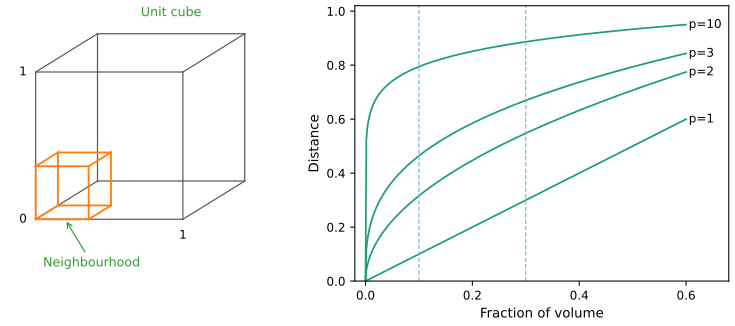
fig_2_6. Reproduces Hastie, Tibshirani and Friedman (2009), Figure 2.6. Download: PDF · SVGAll points are near the edge. Take \(N\) points uniform in the unit ball of \(\R^p\) and a nearest-neighbour estimate at the origin. The median distance to the closest point is
\[ d(p,N)=\Big(1-\tfrac12^{1/N}\Big)^{1/p} \tag{2.24} \](Exercise 2.3). For \(N=500\), \(p=10\), \(d(p,N)\approx0.52\), more than half-way to the boundary: most points are closer to the boundary of the sample space than to any other point, and prediction near the edges must extrapolate rather than interpolate.
Result 2.10 (distance to the nearest neighbour; Exercise 2.3) p. 23, (2.24)
Let \(x_1,\dots,x_N\) be independent and uniform in the unit ball of \(\R^p\) and \(D=\min_i\|x_i\|\). Then \(\Pr(D\gt r)=(1-r^p)^N\) for \(0\le r\le1\), the median of \(D\) is (2.24), and the mean is
\[ \E D=\int_0^1(1-r^p)^N\,\d r=\frac1pB\Big(\frac1p,N+1\Big)=\frac{\Gamma(1+1/p)\,\Gamma(N+1)}{\Gamma(N+1+1/p)}\;\sim\;\Gamma(1+1/p)\,N^{-1/p}. \]Proof
The ball of radius \(r\) has volume \(r^p\) times that of the unit ball, so \(\Pr(\|x_i\|\le r)=r^p\) and \(\Pr(\|x_i\|\gt r)=1-r^p\). The minimum exceeds \(r\) iff every point does, and the points are independent: \(\Pr(D\gt r)=(1-r^p)^N\). The median \(d\) solves \((1-d^p)^N=\tfrac12\), i.e. \(1-d^p=\tfrac12^{1/N}\), which is (2.24). For the mean, \(\E D=\int_0^\infty\Pr(D\gt r)\,\d r\) for a nonnegative variable, and \(D\le1\). Substituting \(u=r^p\), \(\d r=\tfrac1pu^{1/p-1}\d u\):
\[ \int_0^1(1-r^p)^N\d r=\frac1p\int_0^1u^{1/p-1}(1-u)^N\d u=\frac1pB\Big(\frac1p,N+1\Big)=\frac{\Gamma(1/p)\Gamma(N+1)}{p\,\Gamma(N+1+1/p)}, \]and \(\Gamma(1/p)/p=\Gamma(1+1/p)\). The asymptotic form follows from \(\Gamma(N+1)/\Gamma(N+1+a)\sim N^{-a}\). This is the "more complicated expression" for the mean mentioned in the book; it is a beta function. ∎
| \(p\) (with \(N=500\)) | 1 | 2 | 5 | 10 | 20 |
|---|---|---|---|---|---|
| median \(d(p,N)\), (2.24) | 0.0014 | 0.0372 | 0.2681 | 0.5178 | 0.7196 |
| mean \(\E D\) | 0.0020 | 0.0396 | 0.2649 | 0.5110 | 0.7135 |
Bias of 1-NN in high dimensions. Take 1000 training inputs uniform on \([-1,1]^p\) and the noiseless relationship \(Y=f(X)=e^{-8\|X\|^2}\). The 1-NN prediction \(\hat y_0\) of \(f(0)=1\) has mean squared error (over training sets \(\cT\))
\[ \begin{aligned}\MSE(x_0)&=\E_\cT[f(x_0)-\hat y_0]^2\\ &=\E_\cT[\hat y_0-\E_\cT(\hat y_0)]^2+[\E_\cT(\hat y_0)-f(x_0)]^2\\ &=\Var_\cT(\hat y_0)+\Bias^2(\hat y_0),\end{aligned} \tag{2.25} \]the bias-variance decomposition (the cross term vanishes because \(\E_\cT[\hat y_0-\E_\cT\hat y_0]=0\) and the other factor is a constant). Unless the nearest neighbour sits at 0, \(\hat y_0\lt1\), so the estimate is biased downwards. As \(p\) grows the nearest neighbour strays from 0, \(\hat y_0\) tends to 0, the MSE and the squared bias level off at 1, and the variance first grows and then falls.
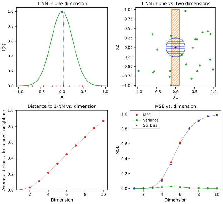
fig_2_7. Reproduces Hastie, Tibshirani and Friedman (2009), Figure 2.7. Download: PDF · SVGFilling the gap 2.5: the exact bias and variance in Figure 2.7 p. 24
The book simulates. In fact the curves follow from the distribution of the nearest-neighbour distance \(R=\min_i\|x_i\|\), because \(\hat y_0=e^{-8R^2}\).
Derivation
For \(r\le1\) the ball of radius \(r\) lies inside the cube \([-1,1]^p\) (of volume \(2^p\)), so for one uniform point \(\Pr(\|x\|\le r)=V_pr^p/2^p\), with \(V_p=\pi^{p/2}/\Gamma(p/2+1)\) the volume of the unit ball; by independence
\[ S(r)=\Pr(R\gt r)=\Big(1-\frac{V_pr^p}{2^p}\Big)^N,\qquad 0\le r\le1 . \]For a differentiable \(g\), \(g(R)=g(0)+\int_0^\infty g'(r)\Ind(R\gt r)\,\d r\); taking expectations (Fubini) gives \(\E g(R)=g(0)+\int_0^\infty g'(r)S(r)\,\d r\). With \(g(r)=e^{-8mr^2}\), \(m=1,2\):
\[ \E\,\hat y_0^{\,m}=1-\int_0^\infty16mr\,e^{-8mr^2}S(r)\,\d r . \]For \(r\gt1\) the ball sticks out of the cube and \(S\) has no simple form, but \(0\le S(r)\le S(1)\) and \(\int_1^\infty16mre^{-8mr^2}\d r=e^{-8m}\), so the part of the integral beyond 1 lies in \([0,e^{-8m}S(1)]\), below \(3.4\times10^{-4}\). The integral over \([0,1]\) is computed by quadrature, and then \(\Bias^2=(1-\E\hat y_0)^2\), \(\Var=\E\hat y_0^2-(\E\hat y_0)^2\). The exact values agree with the simulation within its Monte Carlo error (for \(p=5\): squared bias 0.327 and variance 0.026 exactly, 0.324 and 0.027 simulated). They also confirm the book's statement that for \(p=10\) the nearest neighbour is further than 0.5 from the origin in more than 99% of samples: \(S(0.5)=0.9976\).
The rise and fall of the variance is explained by the same formula: in low dimensions \(R\) is tiny and \(\hat y_0\approx1\) always; in high dimensions \(R\) is large and \(\hat y_0\approx0\) always; only in between (here \(p\approx5\)) does \(\hat y_0\) vary much from sample to sample. This is the "artifact of this example" the book mentions.
Such examples are contrived, but the phenomenon is general: the complexity of functions of many variables can grow exponentially with the dimension, and so must the training set if we want the same accuracy. Whether bias or variance dominates depends on the truth. If \(f\) depends on only a few coordinates the variance can dominate instead, as for \(f(X)=\tfrac12(X_1+1)^3\) in Figure 2.8.
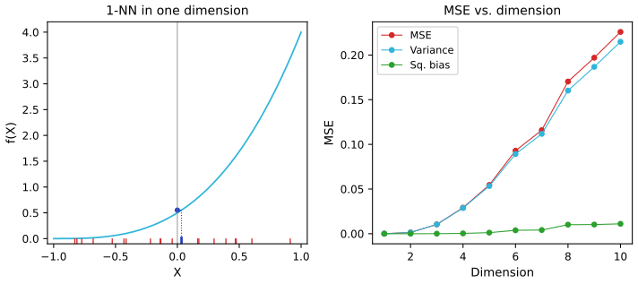
fig_2_8. Reproduces Hastie, Tibshirani and Friedman (2009), Figure 2.8. Download: PDF · SVGFilling the gap 2.6: why the variance dominates in Figure 2.8 p. 24
Derivation
Let \(Z=(Z_1,\dots,Z_p)\) be the nearest training point to the origin and \(R=\|Z\|\). Expanding the cubic around 0,
\[ f(Z)-f(0)=\tfrac32Z_1+\tfrac32Z_1^2+\tfrac12Z_1^3 . \]Reflecting the first coordinate of every training point, \(x\mapsto(-x_1,x_2,\dots,x_p)\), preserves both the uniform distribution on the cube and every norm, so it maps the nearest point to the nearest point and \(Z_1\) has a symmetric distribution: \(\E Z_1=\E Z_1^3=0\). Permuting coordinates likewise shows that \(Z_1,\dots,Z_p\) are exchangeable, so \(\E Z_1^2=\E R^2/p\). Hence, exactly,
\[ \Bias(\hat y_0)=\E f(Z)-f(0)=\tfrac32\E Z_1^2=\frac{3\,\E R^2}{2p}, \]while the variance is dominated by the linear term, \(\Var(\hat y_0)\approx\tfrac94\E Z_1^2\). So \(\Bias^2/\Var\approx\E Z_1^2=\E R^2/p\), which stays small: the nearest point does drift away from 0 as \(p\) grows, but mostly in the \(p-1\) irrelevant directions, and its first coordinate is equally likely to be positive or negative. At \(p=10\) the simulation gives squared bias 0.011 and variance 0.215.
When the model is right. Suppose instead that the relationship is linear,
\[ Y=X^\T\beta+\varepsilon , \tag{2.26} \]with \(\varepsilon\sim\N(0,\sigma^2)\), and we fit by least squares. At a test point \(x_0\), \(\hat y_0=x_0^\T\hat\beta=x_0^\T\beta+\sum_{i=1}^N\ell_i(x_0)\varepsilon_i\), where \(\ell_i(x_0)\) is the \(i\)th entry of \(\bX(\bX^\T\bX)^{-1}x_0\). The estimates are unbiased, and
\[ \begin{aligned}\EPE(x_0)&=\E_{y_0|x_0}\E_\cT(y_0-\hat y_0)^2\\ &=\Var(y_0\given x_0)+\E_\cT[\hat y_0-\E_\cT\hat y_0]^2+[\E_\cT\hat y_0-x_0^\T\beta]^2\\ &=\Var(y_0\given x_0)+\Var_\cT(\hat y_0)+\Bias^2(\hat y_0)\\ &=\sigma^2+\E_\cT x_0^\T(\bX^\T\bX)^{-1}x_0\,\sigma^2+0^2.\end{aligned} \tag{2.27} \]If \(N\) is large, \(\cT\) random and \(\E(X)=0\), then \(\bX^\T\bX\to N\Cov(X)\) and
\[ \begin{aligned}\E_{x_0}\EPE(x_0)&\sim\E_{x_0}x_0^\T\Cov(X)^{-1}x_0\,\sigma^2/N+\sigma^2\\ &=\Tr[\Cov(X)^{-1}\Cov(x_0)]\,\sigma^2/N+\sigma^2\\ &=\sigma^2(p/N)+\sigma^2.\end{aligned} \tag{2.28} \]Result 2.11 (the prediction error of least squares; Exercise 2.5) pp. 24–26, (2.26)–(2.28)
(a) Under (2.26) with errors independent of the inputs, of mean 0 and variance \(\sigma^2\), and a test pair \((x_0,y_0)\) independent of \(\cT\), (2.27) holds; normality is not needed. (b) If \(x_0\) has the distribution of the training inputs and \(\E X=0\), then \[ \E_{x_0}\EPE(x_0)=\sigma^2+\sigma^2\Tr\big(\E[(\bX^\T\bX)^{-1}]\Cov(X)\big), \] which is \(\sigma^2(1+p/N)\) to first order. (c) If the inputs are \(\N(0,\Sigma)\) and \(N\gt p+1\), then exactly
\[ \E_{x_0}\EPE(x_0)=\sigma^2\Big(1+\frac{p}{N-p-1}\Big). \]Proof
(a) Write \(\ell=\bX(\bX^\T\bX)^{-1}x_0\). Since \[ \hat\beta=(\bX^\T\bX)^{-1}\bX^\T(\bX\beta+\varepsilon)=\beta+(\bX^\T\bX)^{-1}\bX^\T\varepsilon, \] we get \(\hat y_0=x_0^\T\beta+\ell^\T\varepsilon\). Conditionally on the inputs \(\bX\), \(\E(\hat y_0\given\bX)=x_0^\T\beta\) and \(\Var(\hat y_0\given\bX)=\sigma^2\ell^\T\ell=\sigma^2x_0^\T(\bX^\T\bX)^{-1}x_0\) (this is \(\Var(\hat\beta\given\bX)=(\bX^\T\bX)^{-1}\sigma^2\), equation (3.8) of the book). By the law of total variance,
\[ \Var_\cT(\hat y_0)=\E\big[\Var(\hat y_0\given\bX)\big]+\Var\big(\E(\hat y_0\given\bX)\big)=\sigma^2\,\E_\cT\,x_0^\T(\bX^\T\bX)^{-1}x_0+0, \]and \(\E_\cT\hat y_0=x_0^\T\beta\): no bias. Finally \(y_0-\hat y_0=(y_0-x_0^\T\beta)-(\hat y_0-x_0^\T\beta)\); the two parts are independent (one depends on the test error, the other on the training data) and the first has mean 0, so the cross term vanishes and \(\E(y_0-\hat y_0)^2=\sigma^2+\Var_\cT(\hat y_0)\).
(b) For a fixed matrix \(A\), \(x_0^\T Ax_0=\Tr(Ax_0x_0^\T)\) (cyclic property), and expectation and trace commute (linearity), so \[ \E_{x_0}x_0^\T Ax_0=\Tr(A\,\E x_0x_0^\T)=\Tr(A\Cov(X)) \] when \(\E X=0\). Apply this with \(A=(\bX^\T\bX)^{-1}\), independent of \(x_0\), after averaging over \(\cT\). Replacing \(\bX^\T\bX\) by \(N\Cov(X)\) gives \(\Tr(\bI_p)/N=p/N\).
(c) If the rows of \(\bX\) are \(\N(0,\Sigma)\), then \(W=\bX^\T\bX=\Sigma^{1/2}W_0\Sigma^{1/2}\) with \(W_0\) the same matrix for standard normal rows, and \(\E W^{-1}=\Sigma^{-1/2}\E(W_0^{-1})\Sigma^{-1/2}\). The distribution of \(W_0\) is unchanged by \(W_0\mapsto QW_0Q^\T\) for orthogonal \(Q\), so \(\E W_0^{-1}=cI\). To find \(c\): \((W_0^{-1})_{11}=1/\mathrm{RSS}_1\), where \(\mathrm{RSS}_1\) is the residual sum of squares of regressing the first column of the standard normal \(\bX_0\) on the other \(p-1\) (the Schur complement); that residual is a standard normal \(N\)-vector projected onto an independent \((N-p+1)\)-dimensional subspace, so \(\mathrm{RSS}_1\sim\chi^2_{N-p+1}\), and \(\E[1/\chi^2_\nu]=1/(\nu-2)\). So \(c=1/(N-p-1)\), \(\E(\bX^\T\bX)^{-1}=\Sigma^{-1}/(N-p-1)\), and (b) gives \(\sigma^2\big(1+\Tr(\bI_p)/(N-p-1)\big)\). ∎
The expected EPE grows linearly in \(p\) with slope \(\sigma^2/N\): negligible if \(N\) is large or \(\sigma^2\) small. By imposing heavy restrictions on the model class, least squares has avoided the curse of dimensionality.
Figure 2.9 compares 1-NN with least squares for \(Y=f(X)+\varepsilon\), \(X\) uniform on \([-1,1]^p\), \(\varepsilon\sim\N(0,1)\), \(N=500\), at \(x_0=0\), for a linear truth \(f(x)=x_1\) and the cubic of Figure 2.8.
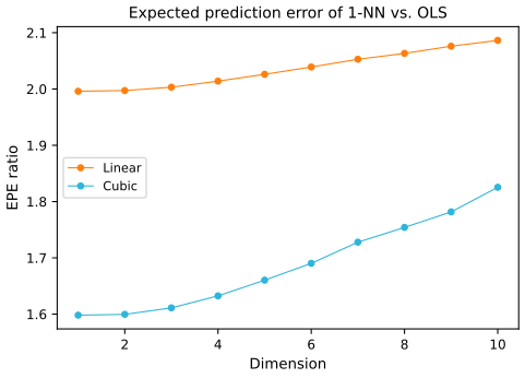
fig_2_9. Reproduces Hastie, Tibshirani and Friedman (2009), Figure 2.9. Download: PDF · SVGFilling the gap 2.7: where the levels 2 and 1.6 in Figure 2.9 come from p. 27
Derivation
1-NN. With \(Z\) the nearest input to 0, \(\hat y_0=f(Z)+\varepsilon_Z\), so \[ \EPE_{\rm 1NN}=\sigma^2+\sigma^2+\E(f(Z)-f(0))^2\ge2\sigma^2=2: \] the noise of the one neighbour is never averaged away. In one dimension \(Z\approx0\) and \(\EPE_{\rm 1NN}\approx2\) for both truths; it grows with \(p\) as \(Z\) strays.
Least squares, linear truth. Unbiased, and with \(x_0=(1,0,\dots,0)\) (intercept first) \(x_0^\T(\bX^\T\bX)^{-1}x_0\approx1/N\) because the inputs are centred, so \(\EPE_{\rm LS}\approx\sigma^2(1+1/N)=1.002\): ratio \(\approx2\), as in the book.
Least squares, cubic truth. The fitted line converges to the best linear approximation (Result 2.5). For \(X_1\) uniform on \([-1,1]\), \(\E X_1=0\), \(\E X_1^2=\tfrac13\), \(\E X_1^4=\tfrac15\), so its intercept is \(\E f(X)=\tfrac12(1+3\cdot\tfrac13)=1\) and its slope is \[ \Cov(X_1,f)/\Var X_1=\tfrac12(3\cdot\tfrac13+\tfrac15)\cdot3=1.8. \] At 0 the line predicts 1 while \(f(0)=\tfrac12\): a bias of 0.5, so \(\EPE_{\rm LS}\approx1+0.25=1.25\) and the ratio starts at \(2/1.25=1.6\). Here least squares is biased, which moderates the ratio; with a stronger nonlinearity 1-NN would win. The simulated values (code output) are 1.0020 and 1.2515 for least squares, and ratios 1.996 to 2.086 (linear) and 1.598 to 1.825 (cubic).
So by relying on rigid assumptions the linear model has no bias and negligible variance when the assumptions hold; if they are wrong, all bets are off. Between rigid linear models and the extremely flexible 1-NN lies a whole spectrum, each with its own assumptions, designed to avoid the exponential growth in complexity.
See also (companion courses): Machine Learning, Section 1.4 (with Result 1.13, volumes of spheres and shells) and Deep Learning, Result 6.1 (volumes, corners and the Gaussian shell), with the high-dimensional geometry demo.
2.6 Statistical Models, Supervised Learning and Function Approximation
p. 28 The goal is a useful approximation \(\hat f(x)\) to the function \(f(x)\) behind the input-output relation. Squared loss leads to the regression function; nearest neighbours estimate it directly but fail in two ways: in high dimensions the neighbours are not close, and when special structure exists, ignoring it wastes data. Other model classes, often designed against the curse of dimensionality, fit into the following framework.
2.6.1 A Statistical Model for the Joint Distribution Pr(X, Y)
pp. 28–29 Suppose the data come from the additive error model
\[ Y=f(X)+\varepsilon , \tag{2.29} \]where \(\E(\varepsilon)=0\) and \(\varepsilon\) is independent of \(X\).
Result 2.12 (what the additive error model implies) pp. 28–29
Under (2.29), \(f(x)=\E(Y\given X=x)\), and the conditional distribution of \(Y\) given \(X=x\) depends on \(x\) only through \(f(x)\): it is the distribution of \(\varepsilon\) shifted by \(f(x)\). For a 0/1 response with \(\Pr(Y=1\given X=x)=p(x)\), by contrast, \(\E(Y\given X=x)=p(x)\) and \(\Var(Y\given X=x)=p(x)[1-p(x)]\): mean and variance are tied together, so an additive model with constant error variance does not fit.
Proof
Independence gives \(\E(\varepsilon\given X)=\E\varepsilon=0\), so \(\E(Y\given X=x)=f(x)\). Also \[ \Pr(Y\le y\given X=x)=\Pr(\varepsilon\le y-f(x)\given X=x)=F_\varepsilon(y-f(x)), \] a function of \(y-f(x)\) only. For a Bernoulli variable \(Y^2=Y\), so \(\Var(Y\given x)=p(x)-p(x)^2\). ∎
The additive model is an approximation: in most systems unmeasured variables and measurement error make the relation non-deterministic, and \(\varepsilon\) absorbs all of that. Some classification problems are deterministic (a coloured map of \(\R^p\)), and the randomness then comes only from where the training inputs fall. Independent identically distributed errors are not essential but sit behind averaging squared errors uniformly; one can let the variance depend on \(x\), for example \(\Var(Y\given X=x)=\sigma^2(x)\).
A slip in the book p. 29
The book writes the heteroscedastic case as \(\Var(Y\given X=x)=\sigma(x)\). A variance is a squared scale, and elsewhere in the chapter \(\sigma^2\) is the variance and \(\sigma\) the standard deviation (for example (2.26), (2.34), (2.46)); the intended statement is \(\Var(Y\given X=x)=\sigma^2(x)\).
2.6.2 Supervised Learning
p. 29 In the machine-learning view, a learning algorithm sees the training inputs \(x_i\), produces outputs \(\hat f(x_i)\), and modifies its input-output relation in response to the differences \(y_i-\hat f(x_i)\): learning by example. After training, the hope is that the artificial and real outputs are close for all inputs likely to be met in practice.
2.6.3 Function Approximation
pp. 29–32 The statistical view treats the pairs \(\{x_i,y_i\}\) as points in \(\R^{p+1}\) and approximates \(f\) on a region of \(\R^p\). Many approximations have parameters \(\theta\); for instance linear basis expansions
\[ f_\theta(x)=\sum_{k=1}^Kh_k(x)\theta_k , \tag{2.30} \]with polynomial or trigonometric \(h_k\) (such as \(x_1^2\), \(x_1x_2^2\), \(\cos(x_1)\)) or nonlinear ones such as the sigmoid of neural networks,
\[ h_k(x)=\frac1{1+\exp(-x^\T\beta_k)} . \tag{2.31} \]Least squares chooses \(\theta\) to minimise
\[ \RSS(\theta)=\sum_{i=1}^N\big(y_i-f_\theta(x_i)\big)^2 , \tag{2.32} \]which has a closed form when the \(h_k\) have no hidden parameters (it is (2.6) with the matrix \(h_k(x_i)\) as \(\bX\)); otherwise iterative optimisation is needed.
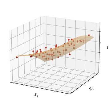
fig_2_10. Reproduces Hastie, Tibshirani and Friedman (2009), Figure 2.10. Download: PDF · SVGA more general principle is maximum likelihood. For a sample \(y_i\) from a density \(\Pr_\theta(y)\), the log-likelihood is
\[ L(\theta)=\sum_{i=1}^N\log\Pr_\theta(y_i), \tag{2.33} \]and the most reasonable \(\theta\) is taken to be the one under which the observed sample is most probable. For the additive model with Gaussian errors,
\[ \Pr(Y\given X,\theta)=\N(f_\theta(X),\sigma^2), \tag{2.34} \] \[ L(\theta)=-\frac N2\log(2\pi)-N\log\sigma-\frac1{2\sigma^2}\sum_{i=1}^N\big(y_i-f_\theta(x_i)\big)^2 . \tag{2.35} \]For a qualitative output with model \(\Pr(G=\mathcal{G}_k\given X=x)=p_{k,\theta}(x)\), the log-likelihood (also called the cross-entropy) is
\[ L(\theta)=\sum_{i=1}^N\log p_{g_i,\theta}(x_i). \tag{2.36} \]Result 2.13 (least squares is Gaussian maximum likelihood; the cross-entropy) pp. 31–32, (2.33)–(2.36)
(a) For every \(\sigma\gt0\), the maximisers of (2.35) over \(\theta\) are the minimisers of \(\RSS(\theta)\); jointly, \(\hat\sigma^2=\RSS(\hat\theta)/N\). (b) (2.36) is the log-likelihood of independent multinomial (categorical) observations. If the model can assign probabilities freely at each distinct input value, (2.36) is maximised by the observed class proportions at each input.
Proof
(a) The log of the normal density \(\N(y_i;f_\theta(x_i),\sigma^2)\) is \(-\tfrac12\log(2\pi)-\log\sigma-(y_i-f_\theta(x_i))^2/(2\sigma^2)\); summing gives (2.35). Only the last term involves \(\theta\), and it is \(-\RSS(\theta)/(2\sigma^2)\), a decreasing function of RSS. With \(\theta=\hat\theta\) plugged in, \(\partial L/\partial\sigma=-N/\sigma+\RSS/\sigma^3=0\) at \(\sigma^2=\RSS/N\), and \(L\to-\infty\) as \(\sigma\to0\) or \(\infty\) (if \(\RSS\gt0\)), so this is the maximum.
(b) \(\Pr(G=g_i\given x_i)=p_{g_i,\theta}(x_i)\), and independence turns the likelihood into a product, the log into the sum (2.36). Group the observations by distinct input value \(x\), with \(n_k\) observations of class \(k\) there and \(n=\sum_kn_k\). Their contribution is \(\sum_kn_k\log q_k\) with \(q_k=p_{k,\theta}(x)\), \(\sum_kq_k=1\). Writing \(\hat q_k=n_k/n\), Gibbs' inequality \(\sum_k\hat q_k\log(\hat q_k/q_k)\ge0\) gives \(\sum_kn_k\log q_k\le\sum_kn_k\log\hat q_k\), with equality iff \(q=\hat q\). ∎
See also (companion courses): Machine Learning, Result 1.9 and Deep Learning, Result 6.7 (error functions as negative log-likelihoods).
2.7 Structured Regression Models
p. 32 Local methods estimate the function at a point directly but struggle in high dimensions, and can be inefficient even in low dimensions when a structured approach would use the data better. Why structure is needed at all:
2.7.1 Difficulty of the Problem
pp. 32–33 Consider minimising, over all functions \(f\),
\[ \RSS(f)=\sum_{i=1}^N\big(y_i-f(x_i)\big)^2 . \tag{2.37} \]Result 2.14 (the unrestricted problem; Exercise 2.6) p. 32, (2.37)
(a) If the \(x_i\) are distinct, the minimisers of (2.37) are exactly the functions that interpolate the data, \(f(x_i)=y_i\): infinitely many, with arbitrary values elsewhere. (b) If the distinct input values \(x_1,\dots,x_n\) carry \(N_i\) observations \(y_{i\ell}\) each, with mean \(\bar y_i\), then
\[ \sum_{i=1}^n\sum_{\ell=1}^{N_i}\big(y_{i\ell}-f(x_i)\big)^2=\sum_{i=1}^n\sum_{\ell=1}^{N_i}(y_{i\ell}-\bar y_i)^2+\sum_{i=1}^nN_i\big(\bar y_i-f(x_i)\big)^2 , \]so the minimisers pass through the averages \(\bar y_i\), and for a parametric family \(f_\theta\) least squares on the full data is equivalent to weighted least squares on the reduced data \((x_i,\bar y_i)\) with weights \(N_i\).
Proof
(a) \(\RSS\ge0\), with equality iff every term vanishes. (b) For each \(i\), write \(y_{i\ell}-f(x_i)=(y_{i\ell}-\bar y_i)+(\bar y_i-f(x_i))\) and expand: the cross term is \(2(\bar y_i-f(x_i))\sum_\ell(y_{i\ell}-\bar y_i)=0\) by the definition of \(\bar y_i\). The first sum does not depend on \(f\), so minimising the left side over any class of functions is the same as minimising \(\sum_iN_i(\bar y_i-f(x_i))^2\), a weighted least-squares criterion on \(n\) points, which is zero at any \(f\) through the averages if \(f\) is unrestricted. ∎
(2.37) is the finite-sample version of (2.11); with enough densely arranged repeats its solutions might tend to the conditional expectation, but for finite \(N\) we must restrict the class of functions. The restriction comes from outside the data (a parametric form, or something built into the method). Any restriction that makes the solution unique only moves the ambiguity to the choice of restriction, since there are infinitely many restrictions.
Most restrictions are complexity restrictions: \(\hat f\) behaves regularly (nearly constant, linear or low-order polynomial) in small neighbourhoods of input space, and the estimate is obtained by averaging or polynomial fitting within a neighbourhood. The size of the neighbourhood sets the strength of the constraint: a local constant fit in infinitesimal neighbourhoods is no constraint at all, a local linear fit in very large neighbourhoods is almost a global linear model. The constraint also depends on the metric. Kernel methods, local regression and trees specify the metric and size of the neighbourhood directly; splines, neural networks and basis-function methods define neighbourhoods implicitly (their equivalent kernels, Section 5.4.1, look like explicit kernels: peaked at the target point and decaying away from it). Any method producing locally varying functions in small isotropic neighbourhoods meets the curse of dimensionality; conversely, every method that overcomes it has a (possibly implicit or adaptive) metric that does not let the neighbourhood be small in all directions at once.
2.8 Classes of Restricted Estimators
pp. 33–34 Nonparametric regression methods fall into overlapping classes according to the restriction they impose. Each has one or more smoothing parameters controlling the effective size of the neighbourhood. Three broad classes:
2.8.1 Roughness Penalty and Bayesian Methods
p. 34 Penalise RSS by a roughness penalty:
\[ \PRSS(f;\lambda)=\RSS(f)+\lambda J(f), \tag{2.38} \]with \(J(f)\) large for functions that vary too rapidly over small regions. The cubic smoothing spline for one-dimensional inputs minimises
\[ \PRSS(f;\lambda)=\sum_{i=1}^N\big(y_i-f(x_i)\big)^2+\lambda\int[f''(x)]^2\,\d x . \tag{2.39} \]Result 2.15 (the two ends of the penalty, and the penalty as a prior) p. 34
(a) Among functions with an absolutely continuous derivative and square-integrable \(f''\), \(\int[f'']^2=0\) iff \(f\) is linear; so as \(\lambda\to\infty\) only linear functions remain affordable, and the limit of the minimiser of (2.39) is the least-squares line. With \(\lambda=0\) every interpolating function minimises (2.39) (Result 2.14). (b) Suppose \(y_i=f(x_i)+\varepsilon_i\) with \(\varepsilon_i\sim\N(0,\sigma^2)\) and a prior density on \(f\) proportional to \(\exp\{-\lambda J(f)/(2\sigma^2)\}\) (made precise below for a finite basis). Then \(-2\sigma^2\log(\text{posterior})=\PRSS(f;\lambda)+\const\), and the minimiser of (2.38) is the posterior mode.
Proof
(a) If \(\int[f'']^2=0\) then \(f''=0\) almost everywhere; \(f'\) is absolutely continuous, so \(f'(x)=f'(a)+\int_a^xf''=f'(a)\) is constant and \(f\) is linear. Conversely linear functions have \(f''=0\). For large \(\lambda\) a minimiser must have \(\lambda J(f)\le\PRSS(\hat f_{\rm line};\lambda)=\RSS(\hat f_{\rm line})\), so \(J\to0\) and the fit approaches the best linear fit; Chapter 5 shows the minimiser is a natural cubic spline and makes this limit exact.
(b) In a finite basis, \(f=\sum_m\theta_mh_m\), a quadratic penalty is \(J(f)=\theta^\T\Omega\theta\) with \(\Omega\) positive semidefinite (for (2.39), \(\Omega_{jk}=\int h_j''h_k''\)). The Gaussian likelihood is \(\propto\exp\{-\RSS(\theta)/(2\sigma^2)\}\) and the prior \(\propto\exp\{-\lambda\theta^\T\Omega\theta/(2\sigma^2)\}\), which is \(\N\big(0,(\sigma^2/\lambda)\Omega^{-1}\big)\) when \(\Omega\) is invertible, and flat (improper) along the null space of \(\Omega\) otherwise (for (2.39), the unpenalised linear functions). By Bayes' theorem the log-posterior is \(-[\RSS(\theta)+\lambda\theta^\T\Omega\theta]/(2\sigma^2)+\const\), so maximising it minimises (2.38). ∎
Penalties can be built in any dimension and to impose special structure: additive penalties \(J(f)=\sum_jJ(f_j)\) with additive functions \(f(X)=\sum_jf_j(X_j)\) give additive models with smooth coordinate functions; projection pursuit regression uses \(f(X)=\sum_{m=1}^Mg_m(\alpha_m^\T X)\) for adaptively chosen directions \(\alpha_m\), each \(g_m\) with its own penalty. Penalties express prior belief in smoothness; this is the Bayesian reading of Result 2.15(b) (Chapters 5 and 8).
See also (companion courses): Machine Learning, Result 1.10 (MAP estimation is regularised least squares) and Deep Learning, Section 4.1.6.
2.8.2 Kernel Methods and Local Regression
pp. 34–35 These methods specify the local neighbourhood explicitly, through a kernel function \(K_\lambda(x_0,x)\) giving weights to points \(x\) around \(x_0\), and the class of functions fitted locally. The Gaussian kernel
\[ K_\lambda(x_0,x)=\frac1\lambda\exp\Big[-\frac{\|x-x_0\|^2}{2\lambda}\Big] \tag{2.40} \]gives weights that die exponentially with squared distance; \(\lambda\), the variance of the Gaussian, sets the width. (The factor \(1/\lambda\) is a convenient normalisation, proportional to the Gaussian density only for \(p=2\); it cancels in everything below.) The simplest kernel estimate is the Nadaraya-Watson weighted average
\[ \hat f(x_0)=\frac{\sum_{i=1}^NK_\lambda(x_0,x_i)y_i}{\sum_{i=1}^NK_\lambda(x_0,x_i)} . \tag{2.41} \]In general a local regression estimate is \(f_{\hat\theta}(x_0)\), where \(\hat\theta\) minimises
\[ \RSS(f_\theta,x_0)=\sum_{i=1}^NK_\lambda(x_0,x_i)\big(y_i-f_\theta(x_i)\big)^2 , \tag{2.42} \]with \(f_\theta\) for instance a low-order polynomial.
Result 2.16 (local constant, local linear, and nearest neighbours as kernels) p. 35
Write \(K_i=K_\lambda(x_0,x_i)\ge0\) with \(\sum_iK_i\gt0\). (a) For \(f_\theta(x)=\theta_0\), the minimiser of (2.42) gives the Nadaraya-Watson estimate (2.41). (b) For scalar \(x\) and \(f_\theta(x)=\theta_0+\theta_1x\), with \(S_j=\sum_iK_i(x_i-x_0)^j\) and \(S_0S_2\gt S_1^2\),
\[ \hat f(x_0)=\sum_{i=1}^N\ell_i(x_0)y_i,\qquad \ell_i(x_0)=\frac{K_i\big[S_2-(x_i-x_0)S_1\big]}{S_0S_2-S_1^2}, \]a linear smoother whose weights sum to 1 and satisfy \(\sum_i\ell_i(x_0)(x_i-x_0)=0\). (c) The \(k\)-NN fit (2.8) is (2.41) with the data-dependent kernel \(K_k(x,x_0)=\Ind\big(\|x-x_0\|\le\|x_{(k)}-x_0\|\big)\), \(x_{(k)}\) the \(k\)th closest training input (if there are no ties at the \(k\)th distance).
Proof
(a) \(\sum_iK_i(y_i-\theta_0)^2\) is a convex quadratic in \(\theta_0\) with derivative \(-2\sum_iK_i(y_i-\theta_0)\), zero at \(\theta_0=\sum_iK_iy_i/\sum_iK_i\).
(b) Reparametrise as \(f(x)=a+b(x-x_0)\), so \(\hat f(x_0)=\hat a\). The weighted normal equations are \(S_0a+S_1b=T_0\), \(S_1a+S_2b=T_1\), with \(T_j=\sum_iK_i(x_i-x_0)^jy_i\). By Cramer's rule \(\hat a=(S_2T_0-S_1T_1)/(S_0S_2-S_1^2)\), which is \(\sum_i\ell_iy_i\) with the stated \(\ell_i\); the determinant is positive by the Cauchy-Schwarz inequality unless all weight sits on one input value. Then \(\sum_i\ell_i=(S_2S_0-S_1^2)/(S_0S_2-S_1^2)=1\) and \(\sum_i\ell_i(x_i-x_0)=(S_2S_1-S_1S_2)/(\cdot)=0\): the weights reproduce linear functions exactly, which is why local linear regression has no first-order bias, also at the boundary (Chapter 6).
(c) With that kernel the weights are 1 on exactly the \(k\) nearest points and 0 elsewhere, so (2.41) is their average. ∎
These methods too must be modified in high dimensions (Chapter 6).
See also (companion course): Machine Learning, Section 6.3.1 (the Nadaraya-Watson model derived from a kernel density estimate).
2.8.3 Basis Functions and Dictionary Methods
pp. 35–36 The model is a linear expansion in basis functions,
\[ f_\theta(x)=\sum_{m=1}^M\theta_mh_m(x), \tag{2.43} \]linear in \(\theta\). The basis may be prescribed (polynomials of total degree \(M\)) or flexible. For one-dimensional \(x\), polynomial splines of degree \(K\) are piecewise polynomials of degree \(K\) between knots, joined with continuous derivatives up to order \(K-1\). For linear splines one basis is \(b_1(x)=1\), \(b_2(x)=x\), \(b_{m+2}(x)=(x-t_m)_+\) for \(m=1,\dots,M-2\), with \(t_m\) the knots and \(z_+\) the positive part.
Result 2.17 (the truncated linear basis spans the linear splines) p. 36
Let \(t_1\lt\dots\lt t_{M-2}\). The \(M\) functions \(1,x,(x-t_1)_+,\dots,(x-t_{M-2})_+\) are linearly independent and span exactly the space of continuous functions that are linear on each of the \(M-1\) intervals determined by the knots.
Proof
Each basis function is continuous and linear between knots, so their combinations are. Conversely, let \(g\) be continuous and linear between knots, with slope \(s_0\) left of \(t_1\), \(s_m\) between \(t_m\) and \(t_{m+1}\), and \(s_{M-2}\) right of \(t_{M-2}\). The function \[ h(x)=a+s_0x+\sum_{m=1}^{M-2}(s_m-s_{m-1})(x-t_m)_+ \] has slope \(s_0+\sum_{m\le j}(s_m-s_{m-1})=s_j\) on the \(j\)th interval, the same as \(g\); two continuous piecewise-linear functions with the same slopes everywhere differ by a constant, which \(a\) removes. For independence: if \(\sum_m\theta_mb_m=0\), the slope jumps by \(\theta_{m+2}\) at \(t_m\), so every \(\theta_{m+2}=0\), and then \(\theta_1+\theta_2x\equiv0\) forces \(\theta_1=\theta_2=0\). ∎
An off-by-one in the book p. 36
The book says that splines of degree \(K\) are represented by \(M\) basis functions "determined in turn by \(M-K\) knots". With \(n\) knots the space of degree-\(K\) splines has dimension \(K+1+n\) (a polynomial of degree \(K\), plus one new coefficient per knot for the jump in the \(K\)th derivative), so \(M\) basis functions need \(n=M-K-1\) knots. The book's own example confirms this: linear splines (\(K=1\)) with \(M\) basis functions use the \(M-2\) knots \(t_1,\dots,t_{M-2}\), not \(M-1\) (Result 2.17); and cubic splines with \(n\) knots have \(n+4\) basis functions (Section 5.2). The count \(M-K\) is correct if \(K\) denotes the order (degree plus one), the convention used in Section 5.2.
Tensor products of spline bases handle more inputs (Section 5.2; CART and MARS in Chapter 9). Radial basis functions are symmetric \(p\)-dimensional kernels at centroids,
\[ f_\theta(x)=\sum_{m=1}^MK_{\lambda_m}(\mu_m,x)\theta_m , \tag{2.44} \]for example the Gaussian \(K_\lambda(\mu,x)=e^{-\|x-\mu\|^2/2\lambda}\). Centroids \(\mu_m\), scales \(\lambda_m\) and spline knots would ideally be chosen by the data too, which turns a linear problem into a combinatorially hard nonlinear one; greedy or two-stage shortcuts are used in practice (Section 6.7). A single-layer feed-forward neural network with linear output weights is an adaptive basis-function method,
\[ f_\theta(x)=\sum_{m=1}^M\beta_m\sigma(\alpha_m^\T x+b_m), \tag{2.45} \]with the activation function \(\sigma(x)=1/(1+e^{-x})\); estimating the directions \(\alpha_m\) and biases \(b_m\) is the main computation (Chapter 11). Methods that choose their basis functions adaptively from a possibly infinite set \(\mathcal{D}\), by some search, are called dictionary methods.
See also (companion courses): Deep Learning, Section 4.1.1 (fixed basis functions) and Section 6.2.2 (universal approximation by (2.45), Result 6.2).
2.9 Model Selection and the Bias-Variance Tradeoff
pp. 37–38 Every model above has a smoothing or complexity parameter: the multiplier of a penalty, the width of a kernel, or the number of basis functions. A smoothing spline ranges from a straight line to an interpolant as \(\lambda\) decreases; a local polynomial ranges from a global polynomial to an interpolant as the window shrinks. The training RSS cannot choose these parameters: it always prefers the interpolating fit. The \(k\)-NN regression fit \(\hat f_k(x_0)\) shows the competing forces. Suppose \(Y=f(X)+\varepsilon\) with \(\E(\varepsilon)=0\), \(\Var(\varepsilon)=\sigma^2\), and, for simplicity, the training inputs \(x_i\) fixed (nonrandom). Then
\[ \begin{aligned}\EPE_k(x_0)&=\E\big[(Y-\hat f_k(x_0))^2\given X=x_0\big]\\ &=\sigma^2+\big[\Bias^2(\hat f_k(x_0))+\Var_\cT(\hat f_k(x_0))\big]\end{aligned} \tag{2.46} \] \[ =\sigma^2+\Big[f(x_0)-\frac1k\sum_{\ell=1}^kf(x_{(\ell)})\Big]^2+\frac{\sigma^2}{k}, \tag{2.47} \]where \(x_{(\ell)}\) is the \(\ell\)th nearest training input to \(x_0\).
Result 2.18 (bias and variance of \(k\)-NN regression) p. 37, (2.46)–(2.47)
Let \(x_1,\dots,x_N\) be fixed, \(y_i=f(x_i)+\varepsilon_i\) with independent errors of mean 0 and variance \(\sigma^2\), and \(Y=f(x_0)+\varepsilon_0\) a new response, independent of the training errors. If the neighbours of \(x_0\) are uniquely defined, (2.46) and (2.47) hold.
Proof
The neighbours depend on the inputs only, which are fixed, so \(\hat f_k(x_0)=\frac1k\sum_\ell y_{(\ell)}=\bar f+\bar\varepsilon\) with \(\bar f=\frac1k\sum_\ell f(x_{(\ell)})\) fixed and \(\bar\varepsilon=\frac1k\sum_\ell\varepsilon_{(\ell)}\). Hence \(\E\hat f_k(x_0)=\bar f\) and \(\Var\hat f_k(x_0)=\Var\bar\varepsilon=\sigma^2/k\), as the \(k\) errors are uncorrelated with variance \(\sigma^2\). Now
\[ Y-\hat f_k(x_0)=\varepsilon_0+\big(f(x_0)-\bar f\big)-\bar\varepsilon . \]The three terms are a zero-mean error, a constant, and a zero-mean error independent of \(\varepsilon_0\), so all cross products have expectation 0 and \(\E(Y-\hat f_k(x_0))^2=\sigma^2+(f(x_0)-\bar f)^2+\sigma^2/k\). ∎
The first term \(\sigma^2\) is the irreducible error, the variance of the new target, beyond our control even if we knew \(f(x_0)\). The other two make up the mean squared error of \(\hat f_k(x_0)\) as an estimate of \(f(x_0)\). The squared bias will most likely grow with \(k\) if \(f\) is smooth: the few nearest neighbours have \(f(x_{(\ell)})\) close to \(f(x_0)\), but as \(k\) grows they are further away and anything can happen. The variance is that of an average and falls like \(1/k\). This is the bias-variance trade-off; more generally, as the model complexity increases, variance tends to rise and squared bias to fall. For \(k\)-NN, complexity is controlled by \(k\), and it is natural to measure it by \(N/k\) (Result 2.2).
We would like to choose the complexity to minimise the test error. The obvious estimate, the training error \(\frac1N\sum_i(y_i-\hat y_i)^2\), does not account for complexity: it keeps decreasing as we fit harder, while the test error eventually rises (Figure 2.11). With too much fitting the model adapts to the training data and generalises badly (large variance, the last term of (2.46)); with too little it underfits (large bias). Chapter 7 discusses how to estimate the test error.
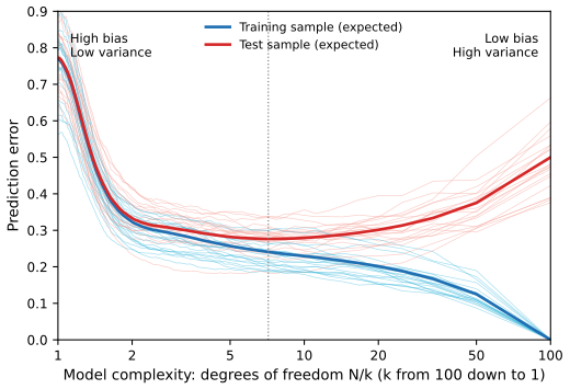
fig_2_11. Reproduces Hastie, Tibshirani and Friedman (2009), Figure 2.11. Download: PDF · SVGFilling the gap 2.8: Figure 2.11 without the hand-waving p. 38
Details
The book's Figure 2.11 is a sketch of "typical behaviour". For \(k\)-NN regression with a fixed design the two curves can be computed exactly. Average Result 2.2 over the design points: with \(b_i(k)=f(x_i)-\frac1k\sum_{x_j\in N_k(x_i)}f(x_j)\) and \(\overline{b^2}(k)=\frac1N\sum_ib_i(k)^2\),
\[ \E[\text{training error}]=\overline{b^2}(k)+\sigma^2\Big(1-\frac1k\Big),\qquad \E[\text{test error}]=\sigma^2+\overline{b^2}(k)+\frac{\sigma^2}k . \]At \(k=1\) (\(N/k=N\)): \(b_i=0\), training error 0, test error \(2\sigma^2=0.5\). At \(k=N\): every fit is the overall mean of the data, and both errors are close to \(\sigma^2+\Var(f(x_i))\approx0.25+0.5\). In between, the test error has a minimum of 0.2763 at \(k=14\), where the training error is 0.2406; the gap is always \(2\sigma^2/k\). The thin curves show that a single data set scatters around these expectations.
See also (companion courses): Deep Learning, Result 4.12 and Machine Learning, Result 3.8 (the bias-variance-noise decomposition for a random training set), with the bias-variance demo for ridge regression.
Bibliographic notes. p. 39 General books on the learning problem include Duda et al. (2000), Bishop (1995, 2006), Ripley (1996), Cherkassky and Mulier (2007) and Vapnik (1996); parts of the chapter follow Friedman (1994).
Exercises
All nine exercises of Chapter 2 (pp. 39–41), restated in my own words, with complete solutions (hidden). Where an exercise needs computation, the method and the result of the Python code are given.
Exercise 2.1. Each of \(K\) classes has a target \(t_k\), the \(k\)th unit vector of \(\R^K\). Show that classifying to the largest element of \(\hat y\) is the same as choosing the closest target, \(\min_k\|t_k-\hat y\|\), if the elements of \(\hat y\) sum to one.
Solution
\[ \|t_k-\hat y\|^2=\|t_k\|^2-2t_k^\T\hat y+\|\hat y\|^2=1-2\hat y_k+\|\hat y\|^2. \] The terms \(1\) and \(\|\hat y\|^2\) do not depend on \(k\), so \(\argmin_k\|t_k-\hat y\|=\argmax_k\hat y_k\) (with the same ties). The condition that the \(\hat y_k\) sum to one is not needed; it only guarantees, for example for least-squares fits with an intercept (Result 2.8), that \(\hat y\) lies on the plane through the targets.
Exercise 2.2. Show how to compute the Bayes decision boundary for the simulation example of Figure 2.5.
Solution
See Filling the gap 2.4. With equal priors and class densities that are equal mixtures of \(\N(m_k,\bI/5)\), the Bayes rule is ORANGE iff \(\sum_{k\in\rm O}e^{-5\|x-m_k\|^2/2}\gt\sum_{k\in\rm B}e^{-5\|x-m_k\|^2/2}\); the boundary is the set where the two sums are equal, computed as the 0.5 contour of \(\Pr(\text{ORANGE}\given x)\) on a fine grid using the 20 means stored with the data (
bayes_probin the code). Its error rate is \(\tfrac12\int\min(f_{\rm B},f_{\rm O})\,\d x=0.2076\) by numerical integration (bayes_error).Exercise 2.3. Derive equation (2.24).
Solution
See Result 2.10: \(\Pr(\min_i\|x_i\|\gt r)=(1-r^p)^N\); setting this equal to \(\tfrac12\) and solving gives \(d(p,N)=(1-\tfrac12^{1/N})^{1/p}\). For \(N=500\), \(p=10\) this is 0.5178. The mean distance is \(B(1/p,N+1)/p=0.5110\).
Exercise 2.4. Let \(X\sim\N(0,\bI_p)\). A prediction point \(x_0\) is drawn from this distribution, \(a=x_0/\|x_0\|\), and the training points \(x_i\) are projected onto \(a\): \(z_i=a^\T x_i\). Show that the \(z_i\) are \(\N(0,1)\) with expected squared distance 1 from the origin, while the target point has expected squared distance \(p\). Hence for \(p=10\) a random test point is about 3.1 standard deviations from the origin, while the training points are on average one standard deviation from it along \(a\): most prediction points see themselves at the edge of the training set.
Solution
The direction \(a\) depends only on \(x_0\), which is independent of the training points. Conditionally on \(x_0\), \(a\) is a fixed unit vector and \(z_i=a^\T x_i\) is a linear combination of independent standard normals with variance \(a^\T\bI a=\|a\|^2=1\): \(z_i\given x_0\sim\N(0,1)\). This conditional distribution does not depend on \(x_0\), so unconditionally \(z_i\sim\N(0,1)\) as well (and the \(z_i\) are independent of each other given \(x_0\)), with \(\E z_i^2=1\). The target point has \(\|x_0\|^2=\sum_jx_{0j}^2\sim\chi^2_p\), so \(\E\|x_0\|^2=p\). For \(p=10\): \(\sqrt{10}=3.16\), and the mean distance itself is \(\E\|x_0\|=\sqrt2\,\Gamma(11/2)/\Gamma(5)=3.08\). Along the line through \(x_0\), the projected training points form a standard normal sample, and the test point sits about 3.1 of their standard deviations out. (The same is true in the direction of any test point, which is the point: in high dimensions, every test point is an outlier in its own direction.)
Exercise 2.5. (a) Derive equation (2.27); the last line uses (3.8) through a conditioning argument. (b) Derive equation (2.28), using the cyclic property and the linearity of the trace.
Solution
See Result 2.11, parts (a) and (b): conditioning on the inputs gives \(\Var(\hat y_0\given\bX)=\sigma^2x_0^\T(\bX^\T\bX)^{-1}x_0\) (this is (3.8)), and the law of total variance with the constant conditional mean \(x_0^\T\beta\) gives (2.27); then \(\E_{x_0}x_0^\T Ax_0=\Tr(A\Cov(X))\) gives (2.28). Part (c) of the result adds the exact value \(\sigma^2(1+p/(N-p-1))\) for Gaussian inputs; a simulation with \(N=50\), \(p=10\) agrees with it (20,000 training sets give 1.260, with Monte Carlo error about 0.004, against \(1+10/39=1.256\) for \(\sigma=1\)), while the first-order formula gives 1.2.
Exercise 2.6. In a regression problem with a parametric model \(f_\theta(x)\) fitted by least squares, show that if some observations have tied (identical) values of \(x\), the fit can be obtained from a reduced weighted least-squares problem.
Solution
See Result 2.14(b): \[ \sum_i\sum_\ell(y_{i\ell}-f_\theta(x_i))^2=\sum_i\sum_\ell(y_{i\ell}-\bar y_i)^2+\sum_iN_i(\bar y_i-f_\theta(x_i))^2, \] and the first sum does not depend on \(\theta\). So \(\hat\theta\) minimises \(\sum_iN_i(\bar y_i-f_\theta(x_i))^2\): weighted least squares on the distinct inputs with responses \(\bar y_i\) and weights \(N_i\). For a linear model, \(\hat\theta=(\bX_r^\T\mathbf{W}\bX_r)^{-1}\bX_r^\T\mathbf{W}\bar{\by}\) with \(\bX_r\) the reduced input matrix and \(\mathbf{W}=\diag(N_i)\) (confirmed numerically to agree with ordinary least squares on the full data).
Exercise 2.7. Let \((x_i,y_i)\) be i.i.d. with \(x_i\sim h(x)\), \(y_i=f(x_i)+\varepsilon_i\), \(\E\varepsilon_i=0\), \(\Var\varepsilon_i=\sigma^2\), and consider estimators linear in the responses, \(\hat f(x_0)=\sum_i\ell_i(x_0;\mathcal{X})y_i\), with weights depending on all the inputs \(\mathcal{X}\) but not on the \(y_i\). (a) Show that linear regression and \(k\)-NN regression are of this form and give their weights. (b) Decompose the conditional mean squared error \(\E_{\mathcal{Y}|\mathcal{X}}(f(x_0)-\hat f(x_0))^2\) into conditional squared bias and conditional variance. (c) Decompose the unconditional mean squared error \(\E_{\mathcal{Y},\mathcal{X}}(f(x_0)-\hat f(x_0))^2\) into squared bias and variance. (d) Relate the squared biases and variances of (b) and (c).
Solution
(a) Least squares: \(\hat f(x_0)=x_0^\T(\bX^\T\bX)^{-1}\bX^\T\by\), so \(\ell_i(x_0;\mathcal{X})\) is the \(i\)th entry of \(\bX(\bX^\T\bX)^{-1}x_0\), i.e. \(\ell_i=x_i^\T(\bX^\T\bX)^{-1}x_0\) (with leading ones for the intercept). \(k\)-NN: \(\ell_i(x_0;\mathcal{X})=\frac1k\Ind\big(x_i\in N_k(x_0)\big)\). In both cases the weights depend on the inputs only.
(b) Given \(\mathcal{X}\), the weights are constants. Let \(\mu(\mathcal{X})=\sum_i\ell_if(x_i)\) be the conditional mean of \(\hat f(x_0)\). Then \(\hat f(x_0)-\mu=\sum_i\ell_i\varepsilon_i\), with mean 0 and variance \(\sigma^2\sum_i\ell_i^2\), and
\[ \E_{\mathcal{Y}|\mathcal{X}}\big(f(x_0)-\hat f(x_0)\big)^2=\underbrace{\big(f(x_0)-\mu(\mathcal{X})\big)^2}_{\text{cond. bias}^2}+\underbrace{\sigma^2\sum_i\ell_i(x_0;\mathcal{X})^2}_{\text{cond. variance}} . \](c) Unconditionally, \(\E\hat f(x_0)=\E_\mathcal{X}\mu(\mathcal{X})=:\bar\mu\), and by the law of total variance \(\Var\hat f(x_0)=\E_\mathcal{X}\big[\sigma^2\sum_i\ell_i^2\big]+\Var_\mathcal{X}\mu(\mathcal{X})\). So
\[ \E_{\mathcal{Y},\mathcal{X}}\big(f(x_0)-\hat f(x_0)\big)^2=\big(f(x_0)-\bar\mu\big)^2+\E_\mathcal{X}\Big[\sigma^2\sum_i\ell_i^2\Big]+\Var_\mathcal{X}\mu(\mathcal{X}). \](d) The unconditional MSE is the average of the conditional one over \(\mathcal{X}\), but the split differs. Since \[ \E_\mathcal{X}(f(x_0)-\mu(\mathcal{X}))^2=(f(x_0)-\bar\mu)^2+\Var_\mathcal{X}\mu(\mathcal{X}), \]
\[ \E_\mathcal{X}[\text{cond. bias}^2]-\text{bias}^2=\text{variance}-\E_\mathcal{X}[\text{cond. variance}]=\Var_\mathcal{X}\Big(\sum_i\ell_i(x_0;\mathcal{X})f(x_i)\Big)\ge0 . \]The averaged conditional squared bias exceeds the unconditional squared bias, and the unconditional variance exceeds the averaged conditional variance, by the same amount: the variability, due to the random design, of the noise-free fit. Confirmed by simulation for \(k\)-NN.
Exercise 2.8. Compare linear regression and \(k\)-NN classification on the zip-code data, using only the 2s and 3s, for \(k=1,3,5,7,15\); give training and test errors. (The data are on the book's website.)
Solution
Method (
zip_two_threein the code). The fileszip.train.gzandzip.test.gzhold \(16\times16\) grey-scale images as 256 inputs. Keeping the digits 2 and 3 leaves 1389 training images (731 twos, 658 threes) and 364 test images. Code \(Y=1\) for a 3 and \(Y=0\) for a 2. Least squares: regress \(Y\) on the 256 pixels with an intercept and classify as 3 when the fit exceeds 0.5. \(k\)-NN: Euclidean distance on the 256 pixels, majority vote, each training point counting itself as a neighbour when computing training error.method training error test error linear regression 0.0058 0.0412 1-NN 0.0000 0.0247 3-NN 0.0050 0.0302 5-NN 0.0058 0.0302 7-NN 0.0065 0.0330 15-NN 0.0094 0.0385 All \(k\)-NN rules beat linear regression on the test set, and here the smallest \(k\) is best: twos and threes are well separated in pixel space, so the low bias of 1-NN outweighs its variance. The training error of linear regression (8 of 1389) is far below its test error (15 of 364), a sign that 257 parameters overfit 1389 images to some extent. My own \(k\)-NN code gives the same predictions as scikit-learn's.
Exercise 2.9. A linear model with \(p\) parameters is fitted by least squares to training data \((x_1,y_1),\dots,(x_N,y_N)\) drawn at random from a population, giving \(\hat\beta\). Test data \((\tilde x_1,\tilde y_1),\dots,(\tilde x_M,\tilde y_M)\) are drawn at random from the same population. With \(R_{tr}(\beta)=\frac1N\sum_1^N(y_i-\beta^\T x_i)^2\) and \(R_{te}(\beta)=\frac1M\sum_1^M(\tilde y_i-\beta^\T\tilde x_i)^2\), prove that \(\E[R_{tr}(\hat\beta)]\le\E[R_{te}(\hat\beta)]\).
Solution
Step 1: \(\E R_{te}(\hat\beta)\) does not depend on \(M\). The test pairs are independent of the training data and of each other, so each term \(\E(\tilde y_i-\hat\beta^\T\tilde x_i)^2\) equals \(\E(\tilde y_1-\hat\beta^\T\tilde x_1)^2\), and their average is that same number. We may therefore take \(M=N\).
Step 2: a symmetry argument. With \(M=N\), let \(\tilde\beta\) be the least-squares estimate computed from the test data. Since the training and test samples have the same distribution, \((\hat\beta,R_{tr})\) and \((\tilde\beta,R_{te})\) are identically distributed, so \(\E R_{tr}(\hat\beta)=\E R_{te}(\tilde\beta)\).
Step 3: optimality. \(\tilde\beta\) minimises \(R_{te}\) over all \(\beta\), in particular \(R_{te}(\tilde\beta)\le R_{te}(\hat\beta)\) for every realisation. Taking expectations, \(\E R_{tr}(\hat\beta)=\E R_{te}(\tilde\beta)\le\E R_{te}(\hat\beta)\). ∎
No model assumptions are needed (only that the expectations are finite). If in addition \(y=x^\T\beta+\varepsilon\) with \(\N(0,\sigma^2)\) errors and Gaussian inputs, both sides are explicit: \(\E R_{tr}(\hat\beta)=\sigma^2(N-p)/N\) (Deep Learning, Result 4.4) and \(\E R_{te}(\hat\beta)=\sigma^2(1+p/(N-p-1))\) (Result 2.11(c)); a simulation confirms both.
Demonstrations for this chapter
Each demonstration runs in the browser and links back to these notes. The ▶ Demo boxes above open them already set to the case under discussion; the simulations use a seeded generator, so a class sees the same pictures.
| Demonstration | What you can see | Sections and results |
|---|---|---|
| Least squares versus k-nearest neighbours on the mixture data | Decision regions for least squares, \(k\)-NN (any odd \(k\)) and the Bayes rule on the book's data; training and test error against \(N/k\) (Figure 2.4). Presets: 1 least squares; 2 15-NN; 3 1-NN; 4 Bayes boundary; 5 best \(k\); 6 \(k=151\). | 2.3, 2.4; Results 2.2, 2.7 |
| The curse of dimensionality | The edge length \(r^{1/p}\); median and mean nearest-neighbour distance (2.24) with simulation; bias and variance of 1-NN at the origin (Figures 2.7 and 2.8). Presets: 1 10% in ten dimensions; 2 1%; 3 (2.24); 4 the bump; 5 the cubic; 6 two dimensions. | 2.5; Results 2.9, 2.10, Gaps 2.5, 2.6 |
| The bias-variance trade-off for k-NN regression | Data, fit and expected fit; (2.47) at a point against \(k\); expected training and test error against \(N/k\) (Figure 2.11). Presets: 1 \(k=1\); 2 \(k=60\); 3 best \(k\) at \(x_0\); 4 Figure 2.11; 5 a jump; 6 more noise. | 2.9, 2.3.2; Results 2.2, 2.18 |
The Python code that produces every figure of this page is code/ch02_overview_supervised_learning.py (see the code index).
References
- Hastie, T., Tibshirani, R. and Friedman, J. (2009). The Elements of Statistical Learning: Data Mining, Inference, and Prediction, 2nd edition. Springer, New York. Chapter 2, pp. 9–41. hastie.su.domains/ElemStatLearn.
- Bellman, R. E. (1961). Adaptive Control Processes: A Guided Tour. Princeton University Press.
- Bishop, C. M. (2006). Pattern Recognition and Machine Learning. Springer, New York.
- Bishop, C. M. and Bishop, H. (2024). Deep Learning: Foundations and Concepts. Springer, Cham.
- Cover, T. M. and Hart, P. E. (1967). Nearest neighbor pattern classification. IEEE Transactions on Information Theory, 13(1), 21–27.
- Friedman, J. H. (1994). An overview of predictive learning and function approximation. In From Statistics to Neural Networks, V. Cherkassky, J. H. Friedman and H. Wechsler (eds), Springer, 1–61.
- Mardia, K. V., Kent, J. T. and Bibby, J. M. (1979). Multivariate Analysis. Academic Press, London (the Wishart distribution and the mean of its inverse).
- Nadaraya, E. A. (1964). On estimating regression. Theory of Probability and Its Applications, 9(1), 141–142.
- Stone, C. J. (1977). Consistent nonparametric regression. Annals of Statistics, 5(4), 595–620.
- Watson, G. S. (1964). Smooth regression analysis. Sankhyā Series A, 26(4), 359–372.
The numerical statements in the text (the least-squares and nearest-neighbour error rates, the Bayes rate, the nearest-neighbour distances, the exact bias and variance of Figures 2.7 to 2.9, the finite-sample prediction error of least squares, the smoother identities and the exercise results) were confirmed numerically.