Smoothing Using Orthogonal Functions
A function in \(\Ltwo\) is determined by its coefficients in an orthonormal basis, and a smooth function needs only a few of them. That turns nonparametric estimation into the estimation of a sequence of means: each coefficient is estimated by an average, and the only real choice is which coefficients to keep. Keeping the first \(J\) (a cosine series) gives estimators whose risk can be estimated without bias and minimised; keeping the large ones wherever they are (wavelet thresholding) adapts to functions that are smooth in some places and rough in others. The book states most of the underlying facts without proof. These notes prove them: completeness of the cosine and Legendre bases, Parseval's relation, the exact risk formulas, the consistency of the noise estimates, Theorem 21.15 with an estimated noise level, and the oracle inequality behind the universal threshold. They also correct the proof of the density band, which tacitly assumes independent coefficients.
Ch. 1 Probability Ch. 2 Random variables Ch. 3 Expectation Ch. 4 Inequalities Ch. 5 Convergence Ch. 6 Models and inference Ch. 7 Estimating the CDF Ch. 8 Bootstrap Ch. 9 Parametric inference Ch. 10 Hypothesis testing Ch. 11 Bayesian inference Ch. 12 Decision theory Ch. 13 Regression Ch. 14 Multivariate models Ch. 15 Independence Ch. 16 Causal inference Ch. 17 Directed graphs Ch. 18 Undirected graphs Ch. 19 Log-linear models Ch. 20 Curve estimation Ch. 21 Orthogonal functions Ch. 22 Classification Ch. 23 Stochastic processes Ch. 24 Simulation
How to read these notes
They follow the book. Sections carry the book's numbers (21.1 to 21.7), numbered equations keep their numbers (\((21.1)\) to \((21.37)\)), and numbered items keep the book's numbers (Examples 21.1 to 21.3, Theorems 21.4 to 21.6, ..., Example 21.16). Results the book uses without a number, and the new results needed to fill its gaps, are lettered (Definition 21.A, Theorem 21.B, ...). The four boxed procedures of the book are Algorithms 21.A to 21.D.
Filling the gaps. Wherever the book says "it can be shown", quotes a result without proof, or leaves an argument implicit, an orange Filling the gap box gives the full argument. Proofs start hidden: open one with its bar, or use the button below.
Indexing. The book counts the cosine basis from \(j=0\) in Section 21.1 and from \(j=1\) elsewhere, and sometimes drops the constant function (the author's errata list this). Here: in Sections 21.1 and 21.2, \(\phi_0=1\) and \(\phi_j(x)=\sqrt2\cos(j\pi x)\); in Section 21.3 the same functions are counted from 1, \(\phi_1=1\) and \(\phi_j(x)=\sqrt2\cos((j-1)\pi x)\), so that "\(J\) terms" means \(\phi_1,\dots,\phi_J\) and the book's sums from 1 are right as printed.
Figures and demonstrations. All eight figures of the chapter are reproduced, and twelve supplementary figures (21.S1 to 21.S12) illustrate gaps and exercises. All are produced by the Python code. The ▶ Demo boxes open an interactive demonstration already set to the case being discussed.
Main reference
L. Wasserman, All of Statistics: A Concise Course in Statistical Inference, Springer (2004), Chapter 21, pages 327–348 (book website: www.stat.cmu.edu/~larry/all-of-statistics). Section, equation, example and exercise numbers below refer to this book. Further reading is listed in the references.
The explanations, derivations, figures and code are my own; equations are cited by their numbers in the book.
Companion courses
Basis expansions and wavelets also appear in companion courses on this site. The overlapping material is:
- Statistical Learning: Theory and Methods, Chapter 5 (basis expansions and regularisation), Section 5.9 (wavelet smoothing): the Haar multiresolution basis (Result 5.14), smoother wavelets (symmlets, Filling the gap 5.11), soft thresholding as the lasso in an orthonormal basis (Result 5.15), the maximum of \(N\) Gaussian noise values (Filling the gap 5.12) and Stein's unbiased risk estimate for soft thresholding (Result 5.16). Its wavelet shrinkage demo compares the universal and SURE thresholds.
- Foundations of Deep Learning, Section 4.1.1 (basis functions), and Bayesian and Probabilistic Machine Learning, Section 2.5 (histograms and kernel density estimators): the other smoothers that this chapter competes with.
- In this course: the histograms, kernel estimators and kernel regression of Chapter 20 (the competing smoothers, with the same bias-variance trade-off and the same rates); Mill's inequality and the Cauchy-Schwarz inequality (Theorems 4.7 and 4.8), the multivariate central limit theorem (Theorem 5.12), Mallows' \(C_p\) (Section 13.6) and Stein's lemma (Lemma 12.C).
Where the companion course proves a result in full (the Haar basis, soft thresholding as the lasso, the Gaussian maximum), these notes give a complete but shorter argument and link to the longer one. New here: completeness of the cosine and Legendre bases (Filling the gaps 21.2 and 21.3), the corrected smoothness identity (21.4), the corrected density band (21.8), the exact variances on the grid (21.9), Theorem 21.15 with an estimated \(\sigma\) (21.16) and the oracle inequality for the universal threshold (Theorem 21.D).
The chapter at a glance
- 21.1 An orthonormal sequence is complete exactly when Parseval's relation \(\norm{f}^2=\sum_j\beta_j^2\) holds for every \(f\) (Theorem 21.B). The cosine basis and the Legendre polynomials are complete. Smoothness means fast decay of the \(\beta_j\).
- 21.2 For a density, \(\bh_j\) is a sample mean of \(\phi_j(X_i)\) (Theorem 21.4). The risk of the \(J\)-term estimate is variance plus tail (Theorem 21.5); it can be estimated, and \(J\) chosen, from the data. A confidence band covers the smoothed density \(f_J\) (Theorem 21.6).
- 21.3 For regression on \(x_i=i/n\), \(\bh_j\) has variance exactly \(\sigma^2/n\); the risk is \(J\sigma^2/n\) plus the tail (Theorem 21.9); the top quarter of the coefficients estimate \(\sigma\); the choice of \(J\) is Mallows' \(C_p\); the band of Theorem 21.11 covers \(r_J\).
- 21.4 Haar wavelets form an orthonormal basis organised by resolution (Theorem 21.13). Keeping only coefficients above the universal threshold \(\sh\sqrt{2\log n/n}\) kills pure noise with probability tending to one (Theorem 21.15) and is within a factor \(2\log n+1\) of an oracle (Theorem 21.D).
- 21.5 The discrete wavelet transform computes all \(n\) Haar coefficients in \(O(n)\) operations.
Notation. \(\ip fg=\int fg\) and \(\norm f=\ip ff^{1/2}\) on the interval in question; \(\beta_j=\ip f{\phi_j}\); \(f_J=\sum_{j\le J}\beta_j\phi_j\) (with the indexing above); \(a_+=\max(a,0)\); \(\chi^2_{J,\alpha}\) is the upper \(\alpha\) quantile of \(\chi^2_J\) and \(\chi_{J,\alpha}\) its square root; \(\Phi\) and \(\phi\) (without index) are the standard Normal cdf and density.
Prerequisites. The central limit theorem (Theorem 5.8) and its multivariate form (Theorem 5.12), the inequalities of Chapter 4, and the regression risk of Section 13.6. See the course home.
21.1 Orthogonal Functions and L2 Spaces
pp. 327–328 In \(\R^3\) every vector is the sum of its projections on three orthonormal vectors, \(v=\sum_j\ip{\psi_j}v\psi_j\) \((21.2)\), whatever orthonormal basis is used. For example \(v=(12,3,4)\) has coefficients \(19/\sqrt3=10.97\), \(9/\sqrt2=6.36\) and \(7/\sqrt6=2.86\) in the basis \(\psi_1,\psi_2,\psi_3\) of the book (Exercise 21.3). The chapter carries this picture over to functions, with sums replaced by integrals.
Definition 21.A (\(\Ltwo\), inner product, orthonormal and complete sequences) pp. 328–329
\(\Ltwo(a,b)\) is the set of (measurable) functions \(f:[a,b]\to\R\) with \(\int_a^bf^2<\infty\) \((21.3)\); two functions that agree except on a set of length zero are identified. The inner product is \(\ip fg=\int_a^bfg\) and the norm is \(\norm f=\sqrt{\ip ff}\) \((21.4)\). A sequence \(\phi_1,\phi_2,\dots\) is orthonormal if \(\ip{\phi_i}{\phi_j}=1\) for \(i=j\) and \(0\) otherwise, and complete if the only \(f\in\Ltwo\) with \(\ip f{\phi_j}=0\) for all \(j\) is \(f=0\). The coefficients of \(f\) are \(\beta_j=\ip f{\phi_j}\) and its partial sums are \(f_n=\sum_{j\le n}\beta_j\phi_j\).
Filling the gap 21.1: the geometry of \(\Ltwo\): best approximation and Bessel's inequality pp. 328–329
Four facts are used throughout the chapter.
- Cauchy-Schwarz. \(|\ip fg|\le\norm f\norm g\), so the inner product is finite on \(\Ltwo\) and \(\norm{f+g}\le\norm f+\norm g\).
- Best approximation. For orthonormal \(\phi_1,\dots,\phi_n\), the combination \(\sum_jc_j\phi_j\) closest to \(f\) has \(c_j=\beta_j\), and \[ \Big\|f-\sum_{j\le n}c_j\phi_j\Big\|^2=\norm f^2-\sum_{j\le n}\beta_j^2+\sum_{j\le n}(c_j-\beta_j)^2 . \]
- Bessel's inequality. \(\sum_j\beta_j^2\le\norm f^2\) for every orthonormal sequence.
- What (21.5) means. "\(f=\sum_j\beta_j\phi_j\)" is a statement about the norm, \(\norm{f-f_n}\to0\) (the book's footnote 1). It does not say that the series converges at every \(x\): the cosine series of a function with a jump overshoots near the jump by about 9% of its size for every \(n\) (Gibbs phenomenon, visible in Figure 21.S8), although the \(\Ltwo\) error tends to zero.
Proofs
(1) For real \(t\), \(0\le\norm{f-tg}^2=\norm f^2-2t\ip fg+t^2\norm g^2\). A quadratic in \(t\) that is never negative has discriminant \(4\ip fg^2-4\norm f^2\norm g^2\le0\). Then \[\norm{f+g}^2=\norm f^2+2\ip fg+\norm g^2\le(\norm f+\norm g)^2\,.\] (The same proof as for random variables, Theorem 4.8.)
(2) Expand the square and use orthonormality: \[\norm{f-\sum c_j\phi_j}^2=\norm f^2-2\sum_jc_j\beta_j+\sum_jc_j^2\,,\] and \(-2c_j\beta_j+c_j^2=(c_j-\beta_j)^2-\beta_j^2\). The last sum is the only term that depends on the \(c_j\), and it is smallest (zero) at \(c_j=\beta_j\).
(3) Take \(c_j=\beta_j\) in (2): \(0\le\norm{f-f_n}^2=\norm f^2-\sum_{j\le n}\beta_j^2\). Let \(n\to\infty\). ∎
Theorem 21.B (Parseval's relation and completeness; Exercise 21.4) p. 329
For an orthonormal sequence \((\phi_j)\) in \(\Ltwo(a,b)\) the following are equivalent:
- the sequence is complete;
- for every \(f\in\Ltwo\), \(\norm{f-f_n}\to0\), that is, (21.5) holds;
- for every \(f\in\Ltwo\), Parseval's relation holds: \[ \norm f^2=\int f^2(x)\,\d x=\sum_{j}\beta_j^2=\norm\beta^2 . \tag{21.6} \]
Then also \(\ip fg=\sum_j\beta_j\gamma_j\) for all \(f,g\) with coefficients \(\beta_j,\gamma_j\).
Proof
(b)\(\iff\)(c): by Filling the gap 21.1(2), \(\norm{f-f_n}^2=\norm f^2-\sum_{j\le n}\beta_j^2\), so one side tends to 0 exactly when the other does.
(a)\(\Rightarrow\)(b): by Bessel's inequality \(\sum_j\beta_j^2<\infty\), so for \(m>n\), \(\norm{f_m-f_n}^2=\sum_{n<j\le m}\beta_j^2\to0\): the partial sums form a Cauchy sequence. \(\Ltwo(a,b)\) is complete as a metric space (the Riesz-Fischer theorem: every Cauchy sequence in \(\Ltwo\) converges in norm; Rudin, 1987, Theorem 3.11), so \(f_n\to g\) for some \(g\in\Ltwo\). The inner product is continuous (Cauchy-Schwarz: \(|\ip{f_n-g}{\phi_k}|\le\norm{f_n-g}\)), so \(\ip g{\phi_k}=\lim_n\ip{f_n}{\phi_k}=\beta_k\). Hence \(f-g\) is orthogonal to every \(\phi_k\), and completeness gives \(f=g\).
(b)\(\Rightarrow\)(a): if \(\ip f{\phi_j}=0\) for every \(j\), all partial sums are 0, and \(\norm f=\lim\norm{f-f_n}=0\).
Finally, apply (21.6) to \(f+g\) and \(f-g\) and subtract: \[4\ip fg=\norm{f+g}^2-\norm{f-g}^2=\sum_j[(\beta_j+\gamma_j)^2-(\beta_j-\gamma_j)^2]=4\sum_j\beta_j\gamma_j\,.\] ∎
Example 21.1 (the cosine basis) p. 329
On \(\Ltwo(0,1)\), \(\phi_0(x)=1\) and \(\phi_j(x)=\sqrt2\cos(j\pi x)\) for \(j\ge1\) \((21.7)\) form a complete orthonormal sequence. The first six are drawn in Figure 21.1.
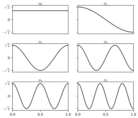
fig_21_1. Download: PDF · SVGFilling the gap 21.2: the cosine basis is orthonormal and complete p. 329
The book states this without proof. Orthonormality is a two-line integral. Completeness reduces, through the substitution \(t=\cos(\pi x)\), to the Weierstrass approximation theorem: polynomials in \(\cos(\pi x)\) are exactly the finite cosine sums.
Proof
Orthonormality. For an integer \(m\ne0\), \(\int_0^1\cos(m\pi x)\,\d x=\sin(m\pi)/(m\pi)=0\). Hence \(\ip{\phi_0}{\phi_j}=0\) for \(j\ge1\), and by \(2\cos A\cos B=\cos(A-B)+\cos(A+B)\), \[ \ip{\phi_j}{\phi_k}=\int_0^1\big[\cos((j-k)\pi x)+\cos((j+k)\pi x)\big]\d x=\begin{cases}1,&j=k\ge1,\\0,&j\ne k.\end{cases} \]
Step 1: cosine sums approximate continuous functions uniformly. Let \(g\) be continuous on \([0,1]\). The map \(x\mapsto t=\cos(\pi x)\) is a continuous bijection from \([0,1]\) onto \([-1,1]\) with continuous inverse \(x=\arccos(t)/\pi\), so \(h(t)=g(\arccos(t)/\pi)\) is continuous on \([-1,1]\) and \(g(x)=h(\cos\pi x)\). By the Weierstrass theorem there is a polynomial \(p\) with \(\sup_t|h(t)-p(t)|<\varepsilon\), hence \(\sup_x|g(x)-p(\cos\pi x)|<\varepsilon\). Each power \(\cos^m\theta\) is a linear combination of \(\cos(k\theta)\), \(0\le k\le m\) (induction with \[\cos\theta\cos k\theta=\tfrac12[\cos((k+1)\theta)+\cos((k-1)\theta)]\]), so \(q(x)=p(\cos\pi x)\) is a finite combination of the \(\phi_j\).
Step 2: completeness. Continuous functions are dense in \(\Ltwo(0,1)\) (Rudin, 1987, Theorem 3.14). Suppose \(\ip f{\phi_j}=0\) for all \(j\) and let \(\varepsilon>0\). Take \(g\) continuous with \(\norm{f-g}<\varepsilon\) and \(q\) as in step 1, so \(\norm{g-q}\le\sup|g-q|<\varepsilon\) and \(\norm{f-q}<2\varepsilon\). Since \(f\) is orthogonal to the finite sum \(q\), \(\norm f^2=\ip f{f-q}\le\norm f\,\norm{f-q}<2\varepsilon\norm f\), so \(\norm f<2\varepsilon\). As \(\varepsilon\) is arbitrary, \(f=0\). ∎
Example 21.2 (the doppler function) pp. 329–330
\(f(x)=\sqrt{x(1-x)}\,\sin\big(2.1\pi/(x+0.05)\big)\) is smooth on the right and oscillates ever faster towards \(x=0\). Figure 21.2 shows its cosine approximations with \(J\) terms. Its coefficients were computed with a midpoint rule on \(2^{20}\) points (one fast cosine transform). With the first \(J\) basis functions \(\phi_0,\dots,\phi_{J-1}\), the squared \(\Ltwo\) errors \(\norm{f-f_J}^2=\norm f^2-\sum_{j<J}\beta_j^2\) are \(0.0645\), \(0.0160\) and \(0.00069\) for \(J=5\), \(20\) and \(200\), against \(\norm f^2=0.0859\). (The book's sum starts at \(j=1\), which drops the constant \(\beta_0=0.048\); see the notes on the book.)
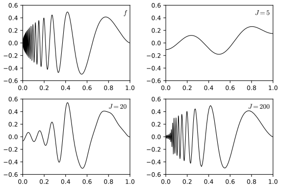
fig_21_2. Download: PDF · SVGExample 21.3 (Legendre polynomials) pp. 329–331
The Legendre polynomials on \([-1,1]\) are given by Rodrigues' formula \[ P_j(x)=\frac1{2^jj!}\frac{\d^j}{\d x^j}(x^2-1)^j,\qquad j=0,1,2,\dots \tag{21.8} \] They are orthogonal and complete, with \(\int_{-1}^1P_j^2=2/(2j+1)\) \((21.9)\), so \(\sqrt{(2j+1)/2}\,P_j\) is an orthonormal basis of \(\Ltwo(-1,1)\). They satisfy \(P_0=1\), \(P_1=x\) and the recursion \[ P_{j+1}(x)=\frac{(2j+1)xP_j(x)-jP_{j-1}(x)}{j+1}. \tag{21.10} \]
Filling the gap 21.3: orthogonality, the norm (21.9), the recursion (21.10) and completeness p. 331
All four facts follow from Rodrigues' formula by integration by parts. The recursion is what the code uses (legendre), and Figure 21.S1 confirms the orthonormality numerically (Exercise 21.5).
Proofs
Write \(u_j=(x^2-1)^j=(x-1)^j(x+1)^j\). Every derivative \(u_j^{(m)}\) with \(m<j\) vanishes at \(\pm1\), since it keeps a factor \((x-1)^{j-m}(x+1)^{j-m}\) in each term. \(P_j\) has degree \(j\) and leading coefficient \(a_j=(2j)!/(2^j(j!)^2)\).
Orthogonality. For \(k<j\), integrate \(\int_{-1}^1x^ku_j^{(j)}\) by parts \(k\) times; the boundary terms vanish, leaving \(\pm k!\int_{-1}^1u_j^{(j-k)}=\pm k!\,[u_j^{(j-k-1)}]_{-1}^{1}=0\). So \(P_j\) is orthogonal to every polynomial of degree below \(j\), in particular to \(P_k\), \(k<j\).
The norm. By orthogonality only the leading term of one factor matters: \(\int P_j^2=a_j\int x^jP_j\). Integrating by parts \(j\) times, \(\int x^ju_j^{(j)}=(-1)^jj!\int u_j=j!\,I_j\) with \(I_j=\int_{-1}^1(1-x^2)^j\). One more integration by parts gives \(I_j=\frac{2j}{2j+1}I_{j-1}\), \(I_0=2\), so \(I_j=2^{2j+1}(j!)^2/(2j+1)!\). Therefore \[ \int_{-1}^1P_j^2=\frac{(2j)!}{2^j(j!)^2}\cdot\frac{j!}{2^jj!}\cdot\frac{2^{2j+1}(j!)^2}{(2j+1)!}=\frac2{2j+1}. \]
The recursion. \(xP_j\) has degree \(j+1\), so \(xP_j=\sum_{k\le j+1}c_kP_k\) with \(c_k=\ip{xP_j}{P_k}/\norm{P_k}^2=\ip{P_j}{xP_k}/\norm{P_k}^2\), which is 0 when \(k+1<j\). \(P_j\) is even or odd with \(j\) (\(u_j\) is even), so \(xP_j\) has the opposite parity and \(c_j=0\). Hence \(xP_j=AP_{j+1}+BP_{j-1}\). Comparing leading coefficients, \(A=a_j/a_{j+1}=(j+1)/(2j+1)\). At \(x=1\), \(u_j^{(j)}(1)=j!\,2^j\) (only the term in which all \(j\) derivatives fall on \((x-1)^j\) survives), so \(P_j(1)=1\) for every \(j\) and \(1=A+B\), \(B=j/(2j+1)\). Multiplying \(xP_j=AP_{j+1}+BP_{j-1}\) by \(2j+1\) gives (21.10).
Completeness. \(P_0,\dots,P_m\) span all polynomials of degree at most \(m\). Polynomials approximate continuous functions uniformly on \([-1,1]\) (Weierstrass), and step 2 of Filling the gap 21.2 applies word for word. ∎
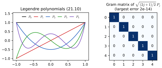
fig_21_s1. Download: PDF · SVGp. 331 The coefficients of a function measure its smoothness. The book writes \(\int_0^1(f^{(k)})^2=2\sum_j\beta_j^2(\pi j)^{2k}\) for the cosine basis; the factor 2 should not be there, and for \(k\ge2\) the identity needs conditions at the end points.
Filling the gap 21.4: smoothness and the decay of the coefficients p. 331
Statement. Let \(f\) be absolutely continuous on \([0,1]\) with \(f'\in\Ltwo\), and let \(\beta_j\) be its cosine coefficients. Then \[ \int_0^1\big(f'(x)\big)^2\,\d x=\sum_{j\ge1}(\pi j)^2\beta_j^2 . \] If moreover \(f'\) is absolutely continuous with \(f''\in\Ltwo\) and \(f'(0)=f'(1)=0\), then \(\int_0^1(f'')^2=\sum_j(\pi j)^4\beta_j^2\); in general, \(\int(f^{(k)})^2=\sum_j(\pi j)^{2k}\beta_j^2\) when the odd derivatives of order below \(k\) vanish at both ends. Without those conditions the cosine coefficients of a smooth function decay only like \(j^{-2}\).
Example. \(f(x)=x\) has \(\beta_j=\sqrt2((-1)^j-1)/(\pi j)^2\), so \(\sum_j(\pi j)^2\beta_j^2=\sum_{j\text{ odd}}8/(\pi j)^2=1=\int_0^1(f')^2\), while the book's formula gives 2. Figure 21.S2 shows the three regimes: a jump gives \(|\beta_j|\sim j^{-1}\), a kink \(j^{-2}\), and even a Gaussian bump, which is infinitely smooth, levels off at \(j^{-2}\) because its slope at the end points is not exactly zero.
Consequence. If \(\sum_j(\pi j)^{2k}\beta_j^2\le C\), the tail beyond \(J\) is small: \[\sum_{j>J}\beta_j^2\le(\pi J)^{-2k}\sum_{j>J}(\pi j)^{2k}\beta_j^2\le C(\pi J)^{-2k}\,.\] This is the quantitative form of the book's "if \(f\) is smooth, the \(\beta_j\) are small for large \(j\)".
Proof
The functions \(s_j(x)=\sqrt2\sin(j\pi x)\), \(j\ge1\), are orthonormal on \([0,1]\) (as in Filling the gap 21.2) and complete: if \(g\perp s_j\) for all \(j\), the odd extension of \(g\) to \([-1,1]\) is orthogonal to every \(\sin(j\pi x)\) and, being odd, to every \(\cos(j\pi x)\), hence zero by completeness of the trigonometric system on \([-1,1]\) (proved like Filling the gap 21.2 with Fejér's theorem in place of Weierstrass; Rudin, 1987, Chapter 4). Integration by parts, with the boundary term \(\big[f\sqrt2\sin(j\pi x)\big]_0^1=0\), gives \[ \ip{f'}{s_j}=-j\pi\int_0^1f(x)\sqrt2\cos(j\pi x)\,\d x=-j\pi\beta_j . \] Parseval's relation in the sine basis (Theorem 21.B) gives the first identity. For the second, integrate by parts again: \[\ip{f''}{\phi_j}=\sqrt2\big[f'(1)(-1)^j-f'(0)\big]-(\pi j)^2\beta_j\] for \(j\ge1\), and \(\ip{f''}{\phi_0}=f'(1)-f'(0)\). These are \(-(\pi j)^2\beta_j\) and 0 exactly when \(f'(0)=f'(1)=0\), and Parseval in the cosine basis gives the identity. If \(f'(0)\) or \(f'(1)\) is not 0, the coefficients cannot decay faster than \(j^{-2}\). Indeed \[(\pi j)^2\beta_j=\sqrt2\big[f'(1)(-1)^j-f'(0)\big]-\ip{f''}{\phi_j}\] with \(\ip{f''}{\phi_j}\to0\) (Bessel), and the bracket is \(\sqrt2(f'(1)-f'(0))\) for even \(j\) and \(-\sqrt2(f'(1)+f'(0))\) for odd \(j\), not both zero; so \(\beta_j\) is of exact order \(j^{-2}\) along even or odd \(j\). Higher orders repeat the argument. ∎
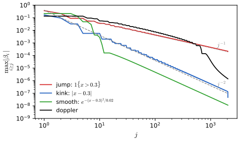
fig_21_s2. Download: PDF · SVG21.2 Density Estimation
See also: histograms and kernel density estimators in Sections 20.2–20.3, and in Section 2.5 of Bayesian and Probabilistic Machine Learning.
pp. 331–332 Let \(X_1,\dots,X_n\) be IID with a density \(f\in\Ltwo(0,1)\). Since \(\int_0^1f=1\), the first coefficient is known, \(\beta_0=\ip f{\phi_0}=1\), and \(f=1+\sum_{j\ge1}\beta_j\phi_j\). Each other coefficient is a mean, \(\beta_j=\int\phi_jf=\E\phi_j(X)\), and is estimated by the sample mean \[ \bh_j=\frac1n\sum_{i=1}^n\phi_j(X_i). \tag{21.11} \]
Theorem 21.4 (mean and variance of \(\bh_j\)) p. 332
\(\E\bh_j=\beta_j\) and \(\V\bh_j=\sigma_j^2/n\) \((21.12)\), where \[ \sigma_j^2=\V\phi_j(X_i)=\int(\phi_j(x)-\beta_j)^2f(x)\,\d x . \tag{21.13} \] For the cosine basis, \(\sigma_j^2=1+\beta_{2j}/\sqrt2-\beta_j^2\le2\).
Proof
The \(\phi_j(X_i)\), \(i=1,\dots,n\), are IID with mean \(\int\phi_jf=\beta_j\), finite because \(|\phi_j|\le\sqrt2\). The mean of \(n\) IID variables has the same mean and \(1/n\) times their variance. For the cosine basis, \[\phi_j^2=2\cos^2(j\pi x)=1+\cos(2j\pi x)=1+\phi_{2j}/\sqrt2\,,\] so \(\E\phi_j^2(X)=1+\beta_{2j}/\sqrt2\) and \(\sigma_j^2=\E\phi_j^2-\beta_j^2\); also \(\sigma_j^2\le\E\phi_j^2\le2\). ∎
The estimate keeps \(J\) terms, \(\fh_J(x)=1+\sum_{j=1}^J\bh_j\phi_j(x)\) \((21.14)\) (the book's display omits the constant 1). The book restricts \(J\) to \(1\le J\le p=\sqrt n\) "for technical reasons", explained in Filling the gap 21.6.
Theorem 21.5 (the risk and its estimate; Exercise 21.1) p. 332
The risk \(R(J)=\E\int(\fh_J-f)^2\) is \[ R(J)=\sum_{j=1}^J\frac{\sigma_j^2}n+\sum_{j=J+1}^\infty\beta_j^2 , \tag{21.15} \] and it is estimated by \[ \Rh(J)=\sum_{j=1}^J\frac{\sh_j^2}n+\sum_{j=J+1}^p\Big(\bh_j^2-\frac{\sh_j^2}n\Big)_+,\qquad \sh_j^2=\frac1{n-1}\sum_{i=1}^n\big(\phi_j(X_i)-\bh_j\big)^2 . \tag{21.16, 21.17} \]
Proof
\(\fh_J-f=\sum_{j\le J}(\bh_j-\beta_j)\phi_j-\sum_{j>J}\beta_j\phi_j\), an \(\Ltwo\) function whose cosine coefficients are \(\bh_j-\beta_j\) for \(1\le j\le J\), \(-\beta_j\) for \(j>J\), and 0 for \(j=0\). By Parseval's relation (Theorem 21.B), \[ \int(\fh_J-f)^2=\sum_{j=1}^J(\bh_j-\beta_j)^2+\sum_{j>J}\beta_j^2 . \] Take expectations: \(\E(\bh_j-\beta_j)^2=\V\bh_j=\sigma_j^2/n\) by Theorem 21.4. For the estimate, \(\sh_j^2\) is the sample variance of the IID \(\phi_j(X_i)\), so \(\E\sh_j^2=\sigma_j^2\), and \(\E\bh_j^2=\beta_j^2+\sigma_j^2/n\), so \(\E(\bh_j^2-\sh_j^2/n)=\beta_j^2\): each term of \(\Rh\) estimates the corresponding term of \(R\) without bias, before the positive part. ∎
Filling the gap 21.5: what the risk estimate estimates, and the price of the positive part pp. 332–333
- Unbiased up to a constant. Without the positive part, \(\tilde R(J)=\sum_{j\le J}\sh_j^2/n+\sum_{J<j\le p}(\bh_j^2-\sh_j^2/n)\) has \(\E\tilde R(J)=R(J)-\sum_{j>p}\beta_j^2\). The missing tail does not depend on \(J\), so \(\tilde R\) and \(R\) have the same expected shape and the same minimiser in expectation.
- A \(C_p\) rule in each step. \(\tilde R(J)-\tilde R(J-1)=2\sh_J^2/n-\bh_J^2\): adding the \(J\)-th term lowers the estimated risk exactly when \(\bh_J^2>2\sh_J^2/n\), that is, when the squared \(t\)-statistic of \(\bh_J\) exceeds 2. This is Mallows' \(C_p\) (or AIC) applied to nested models (Section 13.6). The same holds for \(\Rh\): its increment \(\sh_J^2/n-(\bh_J^2-\sh_J^2/n)_+\) is negative exactly when \(\bh_J^2>2\sh_J^2/n\).
- The positive part. Clipping at 0 respects \(\beta_j^2\ge0\) but adds bias. For a coefficient with \(\beta_j=0\), \(n\bh_j^2/\sigma_j^2\approx Z^2\) with \(Z\sim\N(0,1)\), and \(\E(Z^2-1)_+=2\phi(1)=0.484\): each noise coefficient beyond \(J\) adds about \(0.48\,\sigma_j^2/n\) to \(\Rh(J)\). That bias shrinks as \(J\) grows, which tilts the minimiser slightly upwards. It is visible in Figures 21.S3 and 21.S4, where \(\Rh\) lies above \(R\) near the minimum.
Filling the gap 21.6: how fast, and why \(J\le\sqrt n\) p. 332
Rate. Suppose \(\sum_j(\pi j)^{2k}\beta_j^2\le C\) (a Sobolev-type smoothness of order \(k\), Filling the gap 21.4). Since \(\sigma_j^2\le2\), \[ R(J)\le\frac{2J}n+\frac C{(\pi J)^{2k}} , \] and the choice \(J\asymp n^{1/(2k+1)}\) gives \(R(J)=O\big(n^{-2k/(2k+1)}\big)\): \(n^{-2/3}\) for \(k=1\), \(n^{-4/5}\) for \(k=2\), the same rates as histograms (Theorem 20.4) and kernel estimators (Theorem 20.14) with the matching smoothness.
Why stop at \(p=\sqrt n\). The optimal \(J\asymp n^{1/(2k+1)}\le n^{1/3}\) is far below \(\sqrt n\) for every \(k\ge1\), so the restriction loses nothing. It is needed because the risk estimate is noisy: each term \(\bh_j^2-\sh_j^2/n\) with \(\beta_j\approx0\) has standard deviation of order \(1/n\), so the sum over \(p\) terms fluctuates by about \(\sqrt p/n\). With \(p=\sqrt n\) that is \(n^{-3/4}\), small compared with the risk itself (at least of order \(n^{-2/3}\) when \(k=1\)), so minimising \(\Rh\) is close to minimising \(R\). With \(p\) of order \(n\) the fluctuation would be of order \(n^{-1/2}\), larger than the risk.
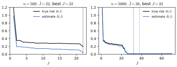
fig_21_s3. Download: PDF · SVGAlgorithm 21.A (orthogonal function density estimation) p. 333
- Compute \(\bh_j=n^{-1}\sum_i\phi_j(X_i)\) and \(\sh_j^2\) for \(j=1,\dots,p=\lfloor\sqrt n\rfloor\).
- Choose \(\hat J\in\{1,\dots,p\}\) to minimise \(\Rh(J)\) of (21.16).
- Estimate \(\fh(x)=1+\sum_{j=1}^{\hat J}\bh_j\phi_j(x)\).
Code: density_series.
p. 333 The estimate can be negative. If a density is needed, the book truncates and renormalises: \(f^*=\max(\fh,0)/\int_0^1\max(\fh,0)\).
Filling the gap 21.7: truncating and renormalising costs little
Write \(\fh^+=\max(\fh,0)\) and \(m=\int\fh^+\). Then (a) \(\norm{\fh^+-f}\le\norm{\fh-f}\), and (b) \(\norm{f^*-f}\le(1+\norm{\fh^+})\norm{\fh-f}\): the repaired estimate has an error of the same order.
Proof
(a) Since \(f\ge0\): where \(\fh\ge0\) nothing changes, and where \(\fh<0\), \(|0-f|=f\le f-\fh=|\fh-f|\). Integrate the squares. (b) \(\int\fh=\beta_0=1\) and \(\fh^+\ge\fh\), so \(m\ge1\), and \[m-1=\int(\fh^+-\fh)=\int_{\{\fh<0\}}(-\fh)\le\int_{\{\fh<0\}}(f-\fh)\le\norm{\fh-f}\] by Cauchy-Schwarz on \([0,1]\). Then \(\norm{f^*-f}\le\norm{f^*-\fh^+}+\norm{\fh^+-f}\), with \[\norm{f^*-\fh^+}=(1-1/m)\norm{\fh^+}\le(m-1)\norm{\fh^+}\,.\] ∎
pp. 333–334 A band for \(f\) itself is out of reach without assumptions on the tail \(\sum_{j>J}\beta_j^2\), so the book gives a band for the smoothed density \(f_J=1+\sum_{j\le J}\beta_j\phi_j\).
Theorem 21.6 (a confidence band for \(f_J\)) pp. 333–334
With \(K=\max_{j\le J}\max_x|\phi_j(x)|\) (\(K=\sqrt2\) for the cosine basis), the book's band is \(\fh_J(x)\pm c\) \((21.18)\) with \[ c=K^2\sqrt{\frac{J\chi^2_{J,\alpha}}n} . \tag{21.19} \] As corrected in Filling the gap 21.8: for fixed \(J\), the band with half-width \(c'=K\sqrt{J\lmax(\Sigma)\chi^2_{J,\alpha}/n}\) has asymptotic coverage at least \(1-\alpha\), where \(\Sigma\) is the covariance matrix of \((\phi_1(X),\dots,\phi_J(X))\); since \(\lmax(\Sigma)\le\sup_xf(x)\), the book's \(c\) is valid when \(\sup f\le K^2\).
Proof
Deterministic step. Let \(L=\sum_{j\le J}(\bh_j-\beta_j)^2\). For every \(x\), by Cauchy-Schwarz in \(\R^J\), \[ |\fh_J(x)-f_J(x)|=\Big|\sum_{j\le J}(\bh_j-\beta_j)\phi_j(x)\Big|\le\Big(\sum_{j\le J}\phi_j(x)^2\Big)^{1/2}\sqrt L\le K\sqrt J\sqrt L . \] Probabilistic step. By the multivariate central limit theorem (Theorem 5.12), \(\sqrt n(\bh-\beta)\rightsquigarrow W\sim\N(0,\Sigma)\), so \(nL\rightsquigarrow\norm W^2\) (continuous mapping). Diagonalise \(\Sigma=\sum_k\lambda_ke_ke_k^\T\): \(\norm W^2=\sum_k\lambda_kZ_k^2\le\lmax\sum_kZ_k^2\) with \(Z_k\) IID \(\N(0,1)\). Hence \[ \lim_n\P\Big(\sup_x|\fh_J-f_J|>c'\Big)\le\lim_n\P\big(nL>\lmax\chi^2_{J,\alpha}\big)=\P\big(\norm W^2>\lmax\chi^2_{J,\alpha}\big)\le\P\big(\chi^2_J>\chi^2_{J,\alpha}\big)=\alpha , \] since \(K\sqrt J\sqrt L>c'\) is the event \(nL>\lmax\chi^2_{J,\alpha}\). With an estimated \(\hat\Sigma\), \(\lmax(\hat\Sigma)\to\lmax(\Sigma)\) in probability and Slutsky's theorem gives the same limit. Finally, for a unit vector \(a\), \[a^\T\Sigma a=\V(\sum a_j\phi_j(X))\le\int(\sum a_j\phi_j)^2f\le\sup f\cdot\int(\sum a_j\phi_j)^2=\sup f\,,\] so \(\lmax\le\sup f\), and \(c'\le c\) when \(\sup f\le K^2\). ∎
Filling the gap 21.8: the proof of Theorem 21.6 treats the \(\bh_j\) as independent pp. 333–334
The book writes \(\bh_j\approx\beta_j+\sigma_j\epsilon_j/\sqrt n\) with \(\epsilon_j\sim\N(0,1)\) and then treats \(\sum_j\sigma_j^2\epsilon_j^2\) as a weighted sum of independent \(\chi^2_1\) variables bounded by \(K^2\chi^2_J\). But \(\bh_j\) and \(\bh_k\) are averages of the same \(X_i\), with covariance \(\Cov(\phi_j(X),\phi_k(X))/n\), which is not zero in general. The correct limit of \(nL\) is \(\sum_k\lambda_kZ_k^2\) with the eigenvalues \(\lambda_k\) of \(\Sigma\), and the bound \(\sigma_j^2\le K^2\) on the diagonal does not bound the eigenvalues.
It matters for the book's own example. For the Bart Simpson density (Example 21.7, \(n=5000\), \(\hat J=38\)) the estimated covariance matrix has \(\lmax=3.09>K^2=2\), because the density reaches about 3.6. The half-width that the argument actually supports is \(c'=1.58\) instead of \(c=1.27\).
It does not matter in practice. The Cauchy-Schwarz step is so generous that both bands are very conservative. In 400 simulated samples (Figure 21.S5), \(\sup_x|\fh_J-f_J|\) never exceeded half of \(c\). Two further caveats apply to any such band: it covers \(f_J\), not \(f\), and it ignores that \(J\) was chosen from the same data.
Example 21.7 (the Bart Simpson density) pp. 334–335
The "claw" of Marron and Wand (1992) is \(f(x)=\tfrac12\phi(x;0,1)+\tfrac1{10}\sum_{l=1}^5\phi(x;\mu_l,0.1)\) with \((\mu_1,\dots,\mu_5)=(-1,-\tfrac12,0,\tfrac12,1)\), where \(\phi(x;\mu,\sigma)\) is the Normal density with standard deviation \(\sigma\). (The book prints the weights \(5/6\) and \(1/6\), which add to \(10/6\); renormalised they are \(1/2\) and \(1/10\).) It is mapped to \([0,1]\) by \(y=(x+3)/6\); the code also discards the 0.13% of draws that fall outside \([0,1]\).
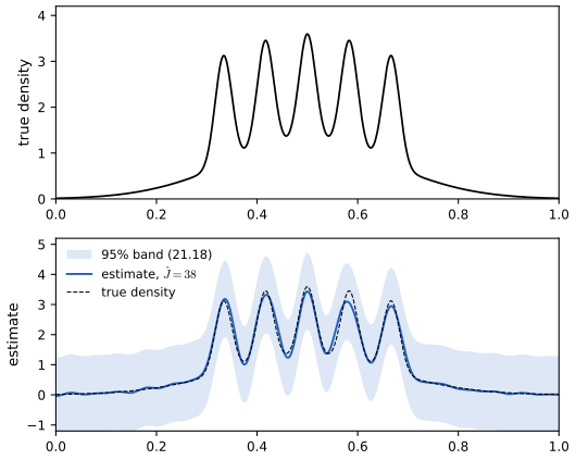
fig_21_3. Download: PDF · SVG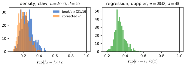
fig_21_s5. Download: PDF · SVG21.3 Regression
See also: kernel regression in Section 20.4; basis expansions in Chapter 5 of Statistical Learning: Theory and Methods.
pp. 335–336 Now \(Y_i=r(x_i)+\epsilon_i\) \((21.21)\) with independent errors of mean 0 and variance \(\sigma^2\), on the grid \(x_i=i/n\). Here the basis is counted from 1: \(\phi_1=1\) and \(\phi_j(x)=\sqrt2\cos((j-1)\pi x)\), so \(r=\sum_{j\ge1}\beta_j\phi_j\) with \(\beta_j=\int_0^1r\phi_j\) \((21.22)\). The coefficients are estimated by \[ \bh_j=\frac1n\sum_{i=1}^nY_i\phi_j(x_i),\qquad j=1,\dots,n. \tag{21.23} \]
Theorem 21.8 (the distribution of \(\bh_j\)) p. 336
\(\bh_j\approx\N(\beta_j,\sigma^2/n)\) \((21.24)\). More precisely (Filling the gap 21.9): \(\E\bh_j=b_j=n^{-1}\sum_ir(x_i)\phi_j(x_i)\), a Riemann sum for \(\beta_j\); \(\V\bh_j=\sigma^2/n\) exactly for \(j=1,\dots,n\); and if the errors are Normal, \(\bh_j\) is exactly Normal.
Proof
\(\E\bh_j=n^{-1}\sum_i\E(Y_i)\phi_j(x_i)=b_j\), and \(b_j\to\int r\phi_j=\beta_j\) as \(n\to\infty\) (a Riemann sum of a Riemann-integrable function). By independence, \[\V\bh_j=n^{-2}\sum_i\sigma^2\phi_j(x_i)^2=(\sigma^2/n)\cdot n^{-1}\sum_i\phi_j(x_i)^2\,,\] and the last average is exactly 1 (Filling the gap 21.9). A linear combination of independent Normals is Normal; without Normality, the Lindeberg central limit theorem applies because the weights \(\phi_j(x_i)/n\) are bounded by \(\sqrt2/n\). ∎
Filling the gap 21.9: on the grid, the variances are exact and the coefficients almost uncorrelated
For integers \(0<m<2n\), \[ \sum_{i=1}^n\cos\Big(\frac{m\pi i}n\Big)=\begin{cases}0,&m\text{ even},\\-1,&m\text{ odd}.\end{cases} \] Consequences, for \(1\le j,l\le n\): \(\sum_i\phi_j(x_i)^2=n\), so \(\V\bh_j=\sigma^2/n\) exactly; and \(\sum_i\phi_j(x_i)\phi_l(x_i)\) is \(0\), \(-2\) or \(-\sqrt2\) for \(j\ne l\), so \(\Cov(\bh_j,\bh_l)=\sigma^2/n^2\) times one of these: the correlations are at most \(2/n\). On the midpoint grid \(x_i=(i-\tfrac12)/n\) the vectors \((\phi_j(x_i))_i\) are exactly orthogonal (the discrete cosine transform of type II), and then \(\bh\) is the least squares fit of the full basis.
The bias. \(b_j-\beta_j\) is the error of a Riemann sum for \(r\phi_j\), of order \(j/n\) for smooth \(r\); it is negligible for \(j\ll n\) but not for \(j\) near \(n\), where frequencies above the grid's resolution fold back (aliasing). For the doppler function with \(n=2048\), \(\sum_{j\le227}(b_j-\beta_j)^2=6\times10^{-11}\).
Proof
With \(z=e^{\mathrm{i}m\pi/n}\ne1\), \(\sum_{i=1}^nz^i=z(1-z^n)/(1-z)\) and \(z^n=(-1)^m\). For even \(m\) the sum is 0. For odd \(m\) it is \(2z/(1-z)\), whose real part is \(-1\) because \(z/(1-z)=-\tfrac12+\tfrac{\mathrm i}2\cot(m\pi/(2n))\) for \(|z|=1\). Now \(\phi_j^2=1+\cos(2(j-1)\pi x)\) for \(j\ge2\), and \(2(j-1)\) is even with \(0<2(j-1)<2n\), so \(\sum_i\phi_j(x_i)^2=n\) (also for \(\phi_1=1\)). For \(j\ne l\), both \(\ge2\), \(\phi_j\phi_l=\cos((j-l)\pi x)+\cos((j+l-2)\pi x)\); the two frequencies have the same parity, giving \(0+0\) or \((-1)+(-1)\). With \(\phi_1=1\), \(\sum_i\sqrt2\cos((l-1)\pi i/n)\) is \(0\) or \(-\sqrt2\). ∎
The estimator keeps \(J\) terms, \(\rh_J(x)=\sum_{j=1}^J\bh_j\phi_j(x)\), with risk \(R(J)=\E\int(\rh_J-r)^2\).
Theorem 21.9 (the risk; Exercise 21.2) p. 336
\[ R(J)=\frac{J\sigma^2}n+\sum_{j=J+1}^\infty\beta_j^2 . \tag{21.25} \]Proof
By Parseval, \(\int(\rh_J-r)^2=\sum_{j\le J}(\bh_j-\beta_j)^2+\sum_{j>J}\beta_j^2\), and \[\E(\bh_j-\beta_j)^2=\V\bh_j+(b_j-\beta_j)^2=\sigma^2/n+(b_j-\beta_j)^2\,.\] So, exactly, \[ R(J)=\frac{J\sigma^2}n+\sum_{j\le J}(b_j-\beta_j)^2+\sum_{j>J}\beta_j^2 , \] and (21.25) holds up to the Riemann-sum term of Filling the gap 21.9. On the midpoint grid there is an exact discrete version: the average squared error at the design points, \(n^{-1}\sum_i\E(\rh_J(x_i)-r(x_i))^2\), equals \(J\sigma^2/n+\sum_{j>J}b_j^2\) exactly, by the discrete Parseval relation for the orthonormal vectors \((\phi_j(x_i)/\sqrt n)_i\). ∎
Filling the gap 21.10: the noise level (21.26) and the risk estimate (21.27) p. 337
The book estimates \(\sigma^2\) from the top quarter of the coefficients, \(k=n/4\): \[ \sh^2=\frac nk\sum_{j=n-k+1}^n\bh_j^2 , \tag{21.26} \] (the printed sum runs over \(i\) but the terms are \(\bh_j\)). By Filling the gap 21.9, \(\E\bh_j^2=\sigma^2/n+b_j^2\) exactly, so \[ \E\sh^2=\sigma^2+\frac nk\sum_{j=n-k+1}^nb_j^2 : \] the bias is the signal left in the top frequencies, \(2.6\times10^{-8}\) for the doppler function with \(n=2048\). If the errors are Normal, the \(\bh_j\) are nearly uncorrelated Normals and \(\V\sh^2\approx2\sigma^4/k\to0\), so \(\sh^2\) is consistent. The risk estimate \[ \Rh(J)=\frac{J\sh^2}n+\sum_{j=J+1}^n\Big(\bh_j^2-\frac{\sh^2}n\Big)_+ \tag{21.27} \] is (21.16) with a common variance, and the remarks of Filling the gap 21.5 apply: each step is a \(C_p\) decision "keep \(\bh_J\) if \(n\bh_J^2/\sh^2>2\)", and the positive part adds about \(0.48\,\sh^2/n\) per pure-noise coefficient. With \(n=2048\) and about 1800 noise coefficients, that is an upward shift of 0.004 near the minimum, visible in Figure 21.S4.
Algorithm 21.B (orthogonal series regression estimator) pp. 337–338
- Compute \(\bh_j=n^{-1}\sum_iY_i\phi_j(x_i)\), \(j=1,\dots,n\).
- Compute \(\sh^2\) by (21.26) (= (21.28)) with \(k\approx n/4\).
- Compute \(\Rh(J)\) by (21.27) for \(1\le J\le n\) and let \(\hat J\) minimise it.
- Estimate \(\rh(x)=\sum_{j=1}^{\hat J}\bh_j\phi_j(x)\).
Code: reg_series, reg_fit.
Example 21.10 (doppler data) p. 337
\(n=2048\) observations \(Y_i=r(i/n)+\epsilon_i\), \(\epsilon_i\sim\N(0,0.1^2)\), with \(r\) the doppler function. For the sample of Figure 21.4, \(\sh=0.0991\) and the risk estimate chooses \(\hat J=227\) terms (the book's sample gave 234). The true risk (21.25) is smallest at \(J=231\), with \(R(231)=1.613\times10^{-3}\) against \(R(227)=1.623\times10^{-3}\).
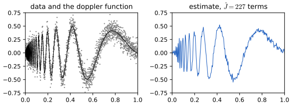
fig_21_4. Download: PDF · SVG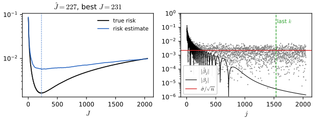
fig_21_s4. Download: PDF · SVGTheorem 21.11 (a confidence band for \(r_J\)) pp. 338–339
Let \(r_J=\sum_{j\le J}\beta_j\phi_j\), with \(J<n-k+1\). The band \(\rh(x)\pm c(x)\) \((21.29)\) with \[ c(x)=\frac{a(x)\,\sh\,\chi_{J,\alpha}}{\sqrt n},\qquad a(x)=\Big(\sum_{j=1}^J\phi_j(x)^2\Big)^{1/2}, \] has asymptotic simultaneous coverage at least \(1-\alpha\) for \(r_J\).
Proof
Let \(L=\sum_{j\le J}(\bh_j-\beta_j)^2\). By Cauchy-Schwarz, \(|\rh(x)-r_J(x)|\le a(x)\sqrt L\) for every \(x\) at once, so \(\sup_x|\rh-r_J|/a(x)\le\sqrt L\). By Theorem 21.8 and Filling the gap 21.9, \((\bh_j-\beta_j)\sqrt n/\sigma\), \(j\le J\), are approximately IID \(\N(0,1)\) (their correlations are \(O(1/n)\) and the biases are negligible for fixed \(J\)), so \(nL/\sigma^2\rightsquigarrow\chi^2_J\). Since \(J<n-k+1\), \(\sh\) uses other coefficients than \(\bh_1,\dots,\bh_J\), and \(\sh\to\sigma\) in probability (Filling the gap 21.10). Hence \[ \P\Big(\sup_x\frac{|\rh(x)-r_J(x)|}{a(x)}>\frac{\sh\chi_{J,\alpha}}{\sqrt n}\Big)\le\P\Big(\frac{nL}{\sh^2}>\chi^2_{J,\alpha}\Big)\to\alpha . \] (The book's last display has \(f\) for \(r\), listed in the author's errata, and \(\beta_j^2\) for \(\beta_j\) inside the square root.) ∎
Filling the gap 21.11: what the band does and does not cover
- Conservative. Equality in Cauchy-Schwarz needs the error vector \(\bh-\beta\) to point along \((\phi_1(x),\dots,\phi_J(x))\) for some \(x\), which almost never happens: in Figure 21.S5 the largest ratio \(\sup_x|\rh-r_J|/c(x)\) in 400 samples is about 0.6. The band is a Scheffé-type band: it would cover every linear combination \(\sum_jc_j(\bh_j-\beta_j)\) at once, not only the evaluations at points \(x\).
- It covers \(r_J\), not \(r\). The half-width grows like \(\sqrt J\cdot\chi_{J,\alpha}/\sqrt n\approx J/\sqrt n\), while the bias \(r-r_J\) shrinks with \(J\). With \(J=45\) in Example 21.12 the band is five times narrower than with \(J=227\), but \(r\) lies inside it at only 88% of the points: it leaves the band where \(x<0.2\).
Example 21.12 (doppler bands) p. 339
Figure 21.5 shows the 95% bands for the data of Figure 21.4 with \(J=\hat J=227\) and \(J=45\approx\sqrt n\); at \(x=0.5\) the half-widths are 0.535 and 0.115.
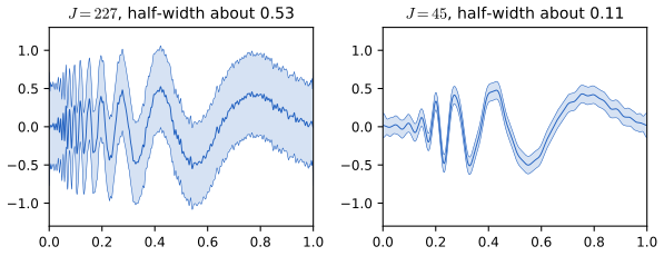
fig_21_5. Download: PDF · SVGFilling the gap 21.12: the shrinkage view, and designs that are not equally spaced p. 339
Shrinkage. Any estimator \(\rh=\sum_jw_j\bh_j\phi_j\) with fixed weights has risk \(\sum_j\big[w_j^2\sigma^2/n+(1-w_j)^2\beta_j^2\big]\) (ignoring the Riemann bias). Three choices of weights:
- Projection, \(w_j=\ind\{j\le J\}\): the method of this section; best risk \(\min_JR(J)\). Doppler, \(n=2048\), \(\sigma=0.1\): \(1.61\times10^{-3}\).
- Keep or kill, any \(w_j\in\{0,1\}\): the best choice keeps \(j\) when \(\beta_j^2>\sigma^2/n\), with risk \(\sum_j\min(\beta_j^2,\sigma^2/n)\). Doppler: \(1.43\times10^{-3}\).
- Ideal linear, \(w_j=\beta_j^2/(\beta_j^2+\sigma^2/n)\): risk \(\sum_j\beta_j^2(\sigma^2/n)/(\beta_j^2+\sigma^2/n)\), between one half and one times the keep-or-kill risk. Doppler: \(1.11\times10^{-3}\).
The last two are oracles: they need the \(\beta_j\). Thresholding (Section 21.4) imitates keep-or-kill from the data, and Theorem 21.D shows how close it gets. Projections lose little for the cosine basis because its coefficients of smooth functions decrease with \(j\); they lose much more for wavelets, whose large coefficients are scattered across levels.
Uneven designs. If the \(x_i\) have a design density \(h\) on \([0,1]\), then \(\E\bh_j\approx\int r\,h\,\phi_j\): the method estimates \(rh\), not \(r\). The book's "the method still applies" needs either \(h\approx1\) or a correction: divide by an estimate of \(h\), or use least squares, or, as in Exercise 21.7, place the sorted observations at \(i/n\) (regression on the ranks) and map back.
21.4 Wavelets
See also: wavelet smoothing in Section 5.9 of Statistical Learning: Theory and Methods, and its wavelet shrinkage demo.
pp. 340–341 A spatially inhomogeneous function, smooth in most places and rough in a few, defeats a single smoothing parameter: few cosine terms miss the rough part, many add wiggles everywhere. Wavelets are localised basis functions, so detail can be added in one place only. The Haar father wavelet (scaling function) and mother wavelet are \[ \phi(x)=\ind\{0<x\le1\},\qquad \psi(x)=\begin{cases}-1,&0<x\le\tfrac12,\\1,&\tfrac12<x\le1,\end{cases}\tag{21.30, 21.31} \] and \(\psi_{j,k}(x)=2^{j/2}\psi(2^jx-k)\) \((21.32)\), supported on the dyadic interval \(I_{j,k}=(k2^{-j},(k+1)2^{-j}]\). (The book closes the intervals on the left; the end points do not matter in \(\Ltwo\), but the convention used here makes the sampled functions at \(x_i=i/n\) match the discrete transform of Section 21.5 exactly.) Let \(W_j=\{\psi_{j,k}:k=0,\dots,2^j-1\}\).
![Left: the mother Haar wavelet, minus 1 on (0, 1/2] and plus 1 on (1/2, 1]. Right: psi_{2,2}, minus 2 on (1/2, 5/8] and plus 2 on (5/8, 3/4].](img/ch21/fig21-6.svg)
fig_21_6. Download: PDF · SVGTheorem 21.13 (the Haar basis) p. 341
\(\{\phi,W_0,W_1,W_2,\dots\}\) is an orthonormal basis of \(\Ltwo(0,1)\). Every \(f\in\Ltwo(0,1)\) is \(f=\alpha\phi+\sum_{j\ge0}\sum_{k=0}^{2^j-1}\beta_{j,k}\psi_{j,k}\) \((21.33)\) with the scaling coefficient \(\alpha=\int f\phi\) and the detail coefficients \(\beta_{j,k}=\int f\psi_{j,k}\). The resolution-\(J\) approximation \[ f_J=\alpha\phi+\sum_{j=0}^{J-1}\sum_{k=0}^{2^j-1}\beta_{j,k}\psi_{j,k}\tag{21.34} \] has \(1+\sum_{j<J}2^j=2^J\) terms, and equals the average of \(f\) over each dyadic interval of length \(2^{-J}\).
Proof (also Exercise 21.8)
Filling the gap 21.13: orthonormality, the multiresolution analysis, and completeness p. 341
The book quotes Theorem 21.13. The whole proof rests on one property of dyadic intervals: two of them are either disjoint or nested, and a smaller one lies inside one half of a larger one. The companion course gives the same result for the Haar case of a general multiresolution analysis (Result 5.14 of Statistical Learning: Theory and Methods).
Proof
Normalisation. \(\psi_{j,k}^2=2^j\) on \(I_{j,k}\), of length \(2^{-j}\), so \(\int\psi_{j,k}^2=1\); also \(\int\phi^2=1\).
Orthogonality. \(\int\psi_{j,k}=2^{j/2}(2^{-j-1}-2^{-j-1})=0\), so \(\psi_{j,k}\perp\phi\). Same level, \(k\ne k'\): disjoint supports. Levels \(j<j'\): \(I_{j',k'}\) is either disjoint from \(I_{j,k}\) or contained in one of its halves, where \(\psi_{j,k}\) is constant, \(\pm2^{j/2}\); then \(\int\psi_{j,k}\psi_{j',k'}=\pm2^{j/2}\int\psi_{j',k'}=0\).
Multiresolution. Let \(V_J\) be the functions constant on each \(I_{J,k}\), \(k=0,\dots,2^J-1\), a space of dimension \(2^J\). Each \(\psi_{j,k}\) with \(j<J\) and \(\phi\) belong to \(V_J\), and they are \(2^J\) orthonormal functions, so they form a basis of \(V_J\): \(V_{J+1}=V_J\oplus\mathrm{span}(W_J)\), the "multiresolution" structure. By Filling the gap 21.1(2), \(f_J\) in (21.34) is the orthogonal projection of \(f\) onto \(V_J\), which is the function equal to \(2^J\int_{I_{J,k}}f\) on \(I_{J,k}\) (the projection onto the indicator of \(I_{J,k}\), normalised).
Completeness. Let \(f\in\Ltwo\) and \(\varepsilon>0\). Take \(g\) continuous with \(\norm{f-g}<\varepsilon\). \(g\) is uniformly continuous on \([0,1]\), so its block averages satisfy \(\sup|g-g_J|\to0\). Projections do not increase norms, so \(\norm{f_J-g_J}\le\norm{f-g}\) and \(\norm{f-f_J}\le2\norm{f-g}+\sup|g-g_J|<3\varepsilon\) for large \(J\). Hence \(f_J\to f\), condition (b) of Theorem 21.B. ∎
Example 21.14 pp. 342–343
Figure 21.7 shows the doppler function and its resolution-\(J\) approximations for \(J=3\), \(5\) and \(8\) (8, 32 and 256 terms). The squared \(\Ltwo\) errors are 0.0372, 0.0123 and 0.00119.
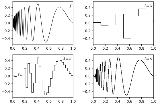
fig_21_7. Download: PDF · SVGp. 342 Haar wavelets are localised but not smooth. Daubechies (1988) constructed wavelets that are both localised (compact support) and smooth, with no closed form; the companion course builds the symmlet filter numerically (Filling the gap 5.11 of Statistical Learning: Theory and Methods). This chapter keeps to Haar wavelets.
pp. 342–344 For regression, \(Y_i=r(x_i)+\sigma\epsilon_i\) with \(x_i=i/n\) and \(n=2^J\). Instead of keeping the first terms, wavelet methods keep the large ones, wherever they are (thresholding). The empirical coefficients are \[ \hat\alpha=\frac1n\sum_i\phi(x_i)Y_i,\qquad D_{j,k}=\frac1n\sum_i\psi_{j,k}(x_i)Y_i,\quad 0\le j\le J-1 \tag{21.35} \] (the book's \(\phi_k\) should be \(\phi\), listed in the author's errata).
Algorithm 21.C (Haar wavelet regression) p. 343
- Compute \(\hat\alpha\) and \(D_{j,k}\) by (21.35), in practice by the discrete wavelet transform (Algorithm 21.D).
- Estimate \(\sigma\) by \[\sh=\sqrt n\,\med\{|D_{J-1,k}|:k=0,\dots,2^{J-1}-1\}/0.6745\] \((21.37)\).
- Universal hard thresholding: \(\bh_{j,k}=D_{j,k}\) if \(|D_{j,k}|>\sh\sqrt{2\log n/n}\), and 0 otherwise \((21.36)\).
- Estimate \(\rh=\hat\alpha\phi+\sum_{j=0}^{J-1}\sum_k\bh_{j,k}\psi_{j,k}\) (the outer sum starts at \(j=0\), listed in the author's errata).
Code: haar_threshold (also soft thresholding, \(\bh_{j,k}=\sign(D_{j,k})(|D_{j,k}|-\lambda)_+\)).
Filling the gap 21.14: the empirical coefficients are exactly independent and equally noisy
At the design points \(x_i=i/n\), each \(I_{j,k}\) contains \(n2^{-j}\) points, half in each half. The dyadic argument of Filling the gap 21.13, with sums over design points instead of integrals, shows that the \(n\) vectors \((\phi(x_i))_i/\sqrt n\) and \((\psi_{j,k}(x_i))_i/\sqrt n\), \(j<J\), are an orthonormal basis of \(\R^n\). Consequences:
- \(D_{j,k}=\tilde\beta_{j,k}+\sigma Z_{j,k}/\sqrt n\) with \(\tilde\beta_{j,k}=n^{-1}\sum_i\psi_{j,k}(x_i)r(x_i)\), and if the errors are Normal the \(Z_{j,k}\) are exactly IID \(\N(0,1)\) (an orthogonal transformation of IID Normals).
- The discrete Parseval relation \(n^{-1}\sum_iY_i^2=\hat\alpha^2+\sum_{j,k}D_{j,k}^2\) holds, and keeping a set of coefficients is a projection in \(\R^n\).
- So the regression problem is exactly a sequence of \(n-1\) Normal means \(\tilde\beta_{j,k}\) observed with common noise \(\sigma/\sqrt n\): the setting of Theorems 21.15 and 21.D.
Filling the gap 21.15: why the noise estimate (21.37) works, and why the median p. 344
At the finest level, \(\psi_{J-1,k}(x_i)=\pm\sqrt{n/2}\) on the two points of \(I_{J-1,k}\), so \[ \sqrt n\,D_{J-1,k}=\frac{Y_{2k+2}-Y_{2k+1}}{\sqrt2}=\frac{r(x_{2k+2})-r(x_{2k+1})}{\sqrt2}+\sigma\frac{\epsilon_{2k+2}-\epsilon_{2k+1}}{\sqrt2} . \] Where \(r\) is continuous the first term is tiny, and the second is \(\N(0,\sigma^2)\) for Normal errors. The median of \(|Z|\) for \(Z\sim\N(0,\sigma^2)\) is \(\sigma\Phi^{-1}(0.75)=0.6745\sigma\), and the sample median of \(n/2\) values converges to it (sample quantiles are consistent at a point where the cdf is strictly increasing), so \(\sh\to\sigma\); in fact \(\sqrt n(\sh-\sigma)\) is asymptotically Normal. The median is used instead of the mean of squares because a few large differences, at jumps or sharp peaks, move a median by a few positions only, while they can dominate a sum of squares (Exercise 21.11 and Figure 21.S12).
Theorem 21.15 (pure noise is removed) p. 344
If \(r=0\) (all \(\beta_{j,k}=0\)) and the errors are Normal, the universal threshold estimator sets every coefficient to 0 with probability tending to 1, both with \(\sigma\) known and with \(\sh\) of (21.37).
Proof (with \(\sigma\) known, as in the book)
By Filling the gap 21.14, the \(n-1\) values \(\sqrt nD_{j,k}/\sigma\) are IID \(\N(0,1)\). With \(\lambda=\sigma\sqrt{2\log n/n}\) and \(t=\sqrt{2\log n}\), the union bound and Mill's inequality \(\P(|Z|>t)\le\sqrt{2/\pi}\,e^{-t^2/2}/t\) (Theorem 4.7) give \[ \P\Big(\max_{j,k}|D_{j,k}|>\lambda\Big)\le(n-1)\,\P(|Z|>t)\le(n-1)\sqrt{\frac2\pi}\,\frac{e^{-\log n}}{\sqrt{2\log n}}\le\frac{\sqrt{2/\pi}}{\sqrt{2\log n}}\to0 . \] ∎
Filling the gap 21.16: Theorem 21.15 with the estimated \(\sigma\), and how slowly it holds p. 344
With \(\sh\). A small underestimate of \(\sigma\) could be fatal, since \(n\,e^{-(1-c)^2\log n}=n^{2c-c^2}\to\infty\) for any fixed \(c>0\). What saves the argument is the rate of \(\sh\): \(\sqrt n(\sh-\sigma)\) is bounded in probability (Filling the gap 21.15). Let \(c_n=n^{-1/4}\) and \(A_n=\{\sh\ge(1-c_n)\sigma\}\); then \(\P(A_n^c)\to0\). On \(A_n\) the threshold is at least \((1-c_n)\sigma\sqrt{2\log n/n}\), and with \(t_n=(1-c_n)\sqrt{2\log n}\), \[ \P\big(\text{some }|D_{j,k}|>\sh\sqrt{2\log n/n}\big)\le\P(A_n^c)+n\sqrt{\frac2\pi}\frac{e^{-t_n^2/2}}{t_n},\qquad n\,e^{-t_n^2/2}=e^{(2c_n-c_n^2)\log n}\to1 , \] because \(c_n\log n\to0\); the factor \(1/t_n\to0\) finishes the proof. (Strictly, \(\sh\) and the coefficients are dependent, since \(\sh\) is computed from the finest level; the union bound above does not need independence.)
How slowly. The exact probability with \(\sigma\) known is \(1-(1-2\bar\Phi(\sqrt{2\log n}))^{n-1}\): 0.245 at \(n=16\), 0.182 at \(n=1024\), 0.159 at \(n=16384\). The bound decreases like \(1/\sqrt{\log n}\), and so does the truth. Why \(\sqrt{2\log n}\): it is the size of the largest of \(n\) independent \(|\N(0,1)|\) values (Filling the gap 5.12 of Statistical Learning: Theory and Methods), so noise sits just below the threshold and signal above it survives.
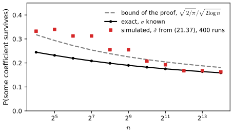
fig_21_s6. Download: PDF · SVGTheorem 21.D (the oracle inequality for universal soft thresholding; Donoho and Johnstone, 1994)
Let \(X\sim\N(\mu,1)\), \(\lambda=\sqrt{2\log n}\) and \(\eta(x)=\sign(x)(|x|-\lambda)_+\). Then \[ \E(\eta(X)-\mu)^2\le(2\log n+1)\Big(\frac1n+\min(\mu^2,1)\Big). \] Consequently, for Haar regression with Normal errors and soft thresholding at \(\sigma\sqrt{2\log n/n}\) (\(\sigma\) known), \[ \sum_{j,k}\E(\bh_{j,k}-\tilde\beta_{j,k})^2\le(2\log n+1)\Big(\frac{\sigma^2}n+\sum_{j,k}\min\Big(\tilde\beta_{j,k}^2,\frac{\sigma^2}n\Big)\Big): \] within a factor \(2\log n+1\) of the keep-or-kill oracle of Filling the gap 21.12, whatever the signal.
Proof
Write \(r(\mu)=\E(\eta(X)-\mu)^2\). Three facts.
(a) \(r(0)\le e^{-\lambda^2/2}=1/n\). Indeed \[\begin{aligned} r(0)&=2\int_\lambda^\infty(x-\lambda)^2\phi(x)\,\d x=2\phi(\lambda)\int_0^\infty t^2e^{-\lambda t-t^2/2}\d t\\ &\le2\phi(\lambda)\int_0^\infty t^2e^{-t^2/2}\d t=2\phi(\lambda)\frac{\sqrt{2\pi}}2=e^{-\lambda^2/2}.\end{aligned}\]
(b) \(r(\mu)\le r(0)+\mu^2\). \(\eta\) is 1-Lipschitz, so we may differentiate under the expectation: \(r'(\mu)=2\E[(\eta(X)-\mu)(\eta'(X)-1)]\), where \(\eta'-1=-\ind\{|X|<\lambda\}\) and \(\eta(X)=0\) on that event; so \(r'(\mu)=2\mu\P(|X|<\lambda)\le2\mu\) for \(\mu\ge0\). Integrate from 0 (and use symmetry for \(\mu<0\)).
(c) \(r(\mu)\le1+\lambda^2\). Write \(\eta(X)=X+g(X)\) with \(g(x)=-\sign(x)\min(|x|,\lambda)\), weakly differentiable with \(g'=-\ind\{|x|<\lambda\}\). Stein's lemma \(\E[(X-\mu)g(X)]=\E g'(X)\) (Lemma 12.C) gives \[r(\mu)=1+2\E g'(X)+\E g(X)^2=\E\big[1-2\ind\{|X|<\lambda\}+\min(X^2,\lambda^2)\big]\le1+\lambda^2\] (Stein's unbiased risk estimate; also Result 5.16 of Statistical Learning: Theory and Methods).
If \(\mu^2\le1\), (a) and (b) give \(r(\mu)\le1/n+\mu^2\le(1+\lambda^2)(1/n+\mu^2)\). If \(\mu^2>1\), (c) gives \(r(\mu)\le1+\lambda^2\le(1+\lambda^2)(1/n+1)\). For the regression statement, \(D_{j,k}=\tilde\beta_{j,k}+(\sigma/\sqrt n)Z_{j,k}\) (Filling the gap 21.14), so \[\E(\bh_{j,k}-\tilde\beta_{j,k})^2=(\sigma^2/n)\,r(\sqrt n\tilde\beta_{j,k}/\sigma)\le(1+\lambda^2)\big(\sigma^2/n^2+\min(\tilde\beta_{j,k}^2,\sigma^2/n)\big)\,;\] sum over the \(n-1\) coefficients. ∎
Hard thresholding, the book's choice, has a bound of the same form with larger constants; Figure 21.S7 compares the two risk functions. Soft thresholding is the lasso in an orthonormal basis (Result 5.15 of Statistical Learning: Theory and Methods). The bound is a guarantee, not a prediction: for the data of Figure 21.8, hard thresholding has average squared error \(3.4\times10^{-3}\) and soft \(7.2\times10^{-3}\) (soft shrinks the large coefficients too), against a keep-or-kill oracle of \(1.3\times10^{-3}\).
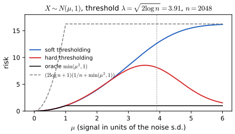
fig_21_s7. Download: PDF · SVGExample 21.16 (Haar regression of doppler data) p. 344
Doppler data with \(\sigma=0.1\), \(n=2048\) (Figure 21.8): \(\sh=0.1031\), \(\lambda=0.0089\), and 59 of the 2047 detail coefficients survive hard thresholding; none at the two finest levels, and at levels 6 to 8 only near \(x=0\), where the function oscillates fast. The estimate is not smooth (Haar wavelets are not), but it follows the oscillations.
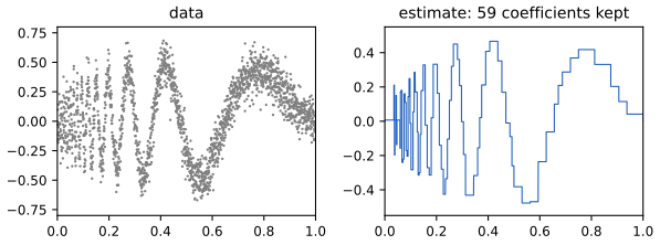
fig_21_8. Download: PDF · SVG21.5 Appendix
Algorithm 21.D (the discrete Haar wavelet transform) p. 345
Input \(y=(Y_1,\dots,Y_n)\), \(n=2^J\). Set \(t\leftarrow y/\sqrt n\). For \(j=J-1,J-2,\dots,0\): with \(m=2^j\) and \(I=1,\dots,m\),
\[ D_j\leftarrow\frac{t[2I]-t[2I-1]}{\sqrt2},\qquad t\leftarrow\frac{t[2I]+t[2I-1]}{\sqrt2}. \]At the end \(t=\hat\alpha\). Code: haar_dwt, and haar_idwt for the inverse.
Filling the gap 21.17: the transform computes (21.35), in \(O(n)\) operations, and is orthogonal
Claim. When level \(j\) is processed, \(t\) has \(2^{j+1}\) entries, the \(m\)-th equal to \(n^{-1/2}2^{-(J-j-1)/2}\) times the sum of \(Y_i\) over the \(m\)-th block of \(n2^{-j-1}\) consecutive points. This holds at the start (\(j=J-1\), blocks of one point), and one step adds neighbouring pairs and divides by \(\sqrt2\), which keeps it true. Hence \[ D_{j,k}=\frac{2^{-(J-j)/2}}{\sqrt n}\Big(\sum_{\text{right half of }I_{j,k}}Y_i-\sum_{\text{left half}}Y_i\Big)=\frac{2^{j/2}}n\Big(\sum_{\text{right}}Y_i-\sum_{\text{left}}Y_i\Big)=\frac1n\sum_i\psi_{j,k}(x_i)Y_i , \] using \(\sqrt n=2^{J/2}\): this is (21.35). The final \(t\) is \(n^{-1/2}2^{-J/2}\sum_iY_i=\hat\alpha\). Each step costs a constant times the current length, so the total is \(n/2+n/4+\dots<n\) pairs. Each step applies the rotation \((a,b)\mapsto((b-a)/\sqrt2,(b+a)/\sqrt2)\) to pairs, an orthogonal map, so the transform of \(y/\sqrt n\) is orthogonal; the inverse undoes the rotations from the coarsest level up. The code's transform agrees with the direct sums (21.35) and its inverse recovers the data to rounding error. ∎
21.6 Bibliographic Remarks
p. 346 Efromovich (1999) treats orthogonal series methods at length; see also Beran (2000) and Beran and Dümbgen (1998) on confidence sets for shrinkage estimators. Ogden (1997) introduces wavelets for statisticians and Härdle, Kerkyacharian, Picard and Tsybakov (1998) go further. Thresholding and its theory are due to Donoho and Johnstone (1994, 1995, 1998) and Donoho, Johnstone, Kerkyacharian and Picard (1995). Smooth compactly supported wavelets are due to Daubechies (1988). The claw density is from Marron and Wand (1992).
Notes on the book
Eight slips of Chapter 21 are in the author's errata lists; the other points are mine, each with the evidence. Page numbers are the book's.
Page 331 and passim: indexing from 0 or 1, and the missing constant
Listed in the author's errata (second list, item 28). The consequence worth spelling out: for a density, (21.14) must read \(\fh=1+\sum_{j=1}^J\bh_j\phi_j\), since the version without the constant integrates to 0; and in Example 21.2 the sum from \(j=1\) omits \(\beta_0=0.048\). These notes use the conventions stated at the top.
Page 331: \(\int(f^{(k)})^2=2\sum_j\beta_j^2(\pi j)^{2k}\) has a spurious factor 2 and needs boundary conditions
For \(f(x)=x\), \(\int(f')^2=1\) while \(2\sum_j\beta_j^2(\pi j)^2=2\). The correct identity has no factor 2, and for \(k\ge2\) needs the odd derivatives below order \(k\) to vanish at 0 and 1 (Filling the gap 21.4). Not in the errata lists.
Page 334, Example 21.7: the weights \(5/6\) and \(1/6\) add to \(10/6\)
With five spikes, \(5/6+5\cdot1/6=10/6\). The claw of Marron and Wand (1992) has weights \(1/2\) and \(1/10\), which is the same mixture renormalised, and matches the heights in Figure 21.3. Not in the errata lists.
Pages 333–334, proof of Theorem 21.6: the coefficients are treated as independent
The bound \(L\lesssim K^2\chi^2_J/n\) needs the largest eigenvalue of the covariance matrix of \((\phi_j(X))_{j\le J}\) to be at most \(K^2\), not only its diagonal; for the claw of Example 21.7 it is 3.09 > 2. Corrected statement and proof in Theorem 21.6 and Filling the gap 21.8. Not in the errata lists.
Page 335, last line: an extra "where"
Listed in the author's errata (first list, item 58).
Page 337: the summation index in (21.26) and (21.28), and the derivation below it
The derivation after (21.26) has \(\bh_j\) where \(Z_j\) is meant: listed in the author's errata (second list, item 29). The sums in (21.26) and (21.28) themselves run over \(i\) while the terms are \(\bh_j\); the index should be \(j\). Not in the errata lists.
Page 339, proof of Theorem 21.11
The last display has \(f\) for \(r\): listed in the author's errata (second list, item 30). The Cauchy-Schwarz line also has \(\sum_j(\bh_j-\beta_j^2)\) for \(\sum_j(\bh_j-\beta_j)^2\). Not in the errata lists.
Page 342: "from" for "form", and "Daubechie"
Listed in the author's errata (first list, items 59 and 60).
Page 343: (21.35) and the outer sum of the Haar estimator
In (21.35), \(\phi_k\) should be \(\phi\), and in step 4 the outer sum should start at \(j=0\): listed in the author's errata (first list, items 62 and 61).
Page 346, Exercise 6: the integral is missing \(\d x\)
Listed in the author's errata (first list, item 63).
Page 348, Exercise 11: the estimator, the claim \(\E(\sh)=\sigma\), and the outlier probability
For \(X_i\sim\N(0,\sigma^2)\) the estimator should be \(\med|X_i|/0.6745\), without the factor \(\sqrt n\) (that factor belongs to (21.37), where \(D\sim\N(0,\sigma^2/n)\)). Even then \(\E\sh=\sigma\) holds only in the limit: for \(n=100\), \(\E\sh=1.0033\sigma\) (simulation). In (c), "with probability .95" appears twice; the outliers should have probability .05. Not in the errata lists.
21.7 Exercises
All twelve exercises of Chapter 21 (Wasserman, 2004, pp. 346–348), restated in my own words, with complete solutions (hidden).
Exercise 21.1. Prove Theorem 21.5.
Solution
See the proof of Theorem 21.5: Parseval's relation turns the integrated squared error into \(\sum_{j\le J}(\bh_j-\beta_j)^2+\sum_{j>J}\beta_j^2\), and Theorem 21.4 gives the expectation. The unbiasedness of the pieces of \(\Rh\) is shown there too, and Filling the gap 21.5 discusses the positive part. A simulation of 600 samples of size 5000 from the claw with \(J=20\) gives a mean integrated squared error within 2% of (21.15).
Exercise 21.2. Prove Theorem 21.9.
Solution
See the proof of Theorem 21.9, which gives the exact risk \(J\sigma^2/n+\sum_{j\le J}(b_j-\beta_j)^2+\sum_{j>J}\beta_j^2\) using the exact variance of Filling the gap 21.9, and the exact discrete version on the midpoint grid.
Exercise 21.3. Show that \(\psi_1=(1,1,1)/\sqrt3\), \(\psi_2=(1,-1,0)/\sqrt2\) and \(\psi_3=(1,1,-2)/\sqrt6\) have norm 1 and are orthogonal.
Solution
\(\norm{\psi_1}^2=3/3\), \(\norm{\psi_2}^2=2/2\), \(\norm{\psi_3}^2=(1+1+4)/6\), all 1. \(\ip{\psi_1}{\psi_2}=(1-1+0)/\sqrt6=0\), \(\ip{\psi_1}{\psi_3}=(1+1-2)/\sqrt{18}=0\), \(\ip{\psi_2}{\psi_3}=(1-1+0)/\sqrt{12}=0\). Three orthonormal vectors in \(\R^3\) are linearly independent, hence a basis. For \(v=(12,3,4)\): \(\ip{\psi_1}v=19/\sqrt3=10.97\), \(\ip{\psi_2}v=9/\sqrt2=6.36\), \(\ip{\psi_3}v=7/\sqrt6=2.86\), as on p. 328, and \(10.97^2+6.36^2+2.86^2=169=\norm v^2\) (Parseval).
Exercise 21.4. Prove Parseval's relation (21.6).
Solution
For a complete orthonormal sequence, (21.6) is (a)\(\Rightarrow\)(c) of Theorem 21.B; the proof there uses Bessel's inequality, the completeness of \(\Ltwo\) as a metric space and the definition of a complete sequence. For an orthonormal sequence that is not complete, only Bessel's inequality \(\sum\beta_j^2\le\norm f^2\) holds.
Exercise 21.5. Plot the first five Legendre polynomials and check numerically that the normalised versions are orthonormal.
Solution
Figure 21.S1: \(P_0,\dots,P_4\) from the recursion (21.10) (they agree with the library values to \(10^{-14}\)), and the Gram matrix of \(\sqrt{(2j+1)/2}P_j\), equal to the identity within \(2\times10^{-14}\). The proof is Filling the gap 21.3.
Exercise 21.6. Expand in the cosine basis of \([0,1]\): (a) \(\sqrt2\cos(3\pi x)\); (b) \(\sin(\pi x)\) (coefficients analytically); (c) the "blocks" function \(\sum_{j=1}^{11}h_jK(x-t_j)\) with \(K(t)=(1+\sign t)/2\) and the book's jump points \(t_j\) and heights \(h_j\); (d) the doppler function (coefficients numerically, by \(N^{-1}\sum_{r=1}^Nf(r/N)\phi_j(r/N)\)). Plot partial sums for increasing numbers of terms.
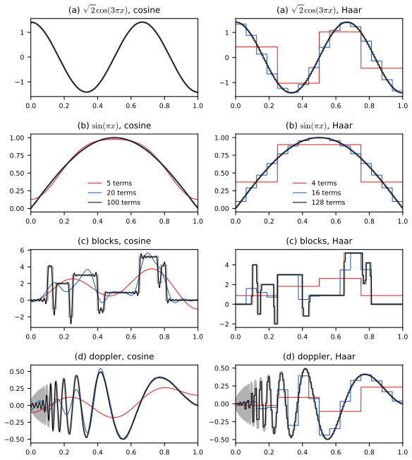
Figure 21.S8 (supplementary). Exercises 21.6 and 21.12: partial sums in the cosine basis (left, 5, 20 and 100 terms) and in the Haar basis (right, 4, 16 and 128 terms) for the four functions; the true function is the thick grey line. Not a figure of the book. Code: fig_21_s8. Download: PDF · SVGSolution
(a) \(\sqrt2\cos(3\pi x)=\phi_3\), so \(\beta_3=1\) and every other coefficient is 0; the expansion is exact from four terms on. (The Riemann sums of the exercise reproduce this only up to errors of order \(1/N\), because the cosines are not exactly orthogonal on the grid \(r/N\); see Filling the gap 21.9.)
(b) \(\beta_0=\int_0^1\sin\pi x=2/\pi\). For \(j\ge1\), \[\int_0^1\sin(\pi x)\cos(j\pi x)\,\d x=(1+(-1)^j)/(\pi(1-j^2))\] (product to sum), so \(\beta_j=2\sqrt2/(\pi(1-j^2))\) for even \(j\) and \(0\) for odd \(j\). The decay is \(j^{-2}\), as Filling the gap 21.4 predicts (\(f'(0)=\pi\ne0\)); the numerical coefficients agree to \(10^{-7}\).
(c) In closed form, \(\beta_0=\sum_jh_j(1-t_j)\) and \(\beta_m=-\sqrt2\sum_jh_j\sin(m\pi t_j)/(m\pi)\) for \(m\ge1\). They decay only like \(1/m\), and the partial sums ring at each jump (Gibbs phenomenon) however many terms are kept.
(d) The doppler coefficients stay of order \(10^{-2}\) to \(10^{-3}\) up to \(j\approx700\) (Figure 21.S2), so even 100 terms miss the oscillations near 0. With \(N=4096\) the Riemann-sum coefficients agree with the fine midpoint rule to about \(10^{-4}\).
Exercise 21.7. Glass fragments data: \(Y\) is the refractive index and \(X\) the aluminium content. (a) Fit \(Y=f(X)+\epsilon\) with the cosine basis, ignoring the irregular spacing of the \(X\) (after sorting); give the estimate, the estimated risk and a confidence band. (b) Fit it with wavelets.
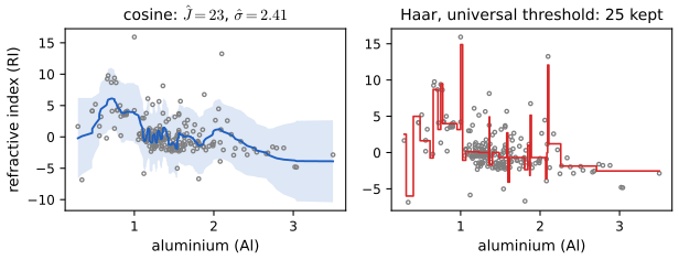
Figure 21.S9 (supplementary). Exercise 21.7: cosine fit with 23 terms and 95% band (left), and Haar fit with universal hard thresholding (right), for the 214 glass fragments. Not a figure of the book. Code: fig_21_s9. Download: PDF · SVGSolution
The 214 fragments are sorted by aluminium (ties broken by refractive index) and placed at \(x_i=i/n\), which is what "ignore the spacing" means in practice; plugging the rescaled aluminium values into \(\phi_j(x_i)\) instead would estimate \(r\) times the design density (Filling the gap 21.12). (a) With \(k=53\), \(\sh=2.41\); the risk estimate is minimised at \(\hat J=23\), with \(\Rh(23)=3.56\); the median half-width of the 95% band is 4.6. Refractive index decreases with aluminium, from about 5 at Al \(\approx0.7\) to about \(-4\) at Al \(\approx3.5\); the wiggles of the fit lie well inside the band. (b) 214 is not a power of 2, so the sorted responses are extended to 256 by mirror reflection; then \(\sh=1.38\) and 25 coefficients survive the universal threshold. The Haar fit picks out a few isolated fragments with extreme refractive index as spikes. The two noise estimates differ because the cosine estimate (21.26) also absorbs these outliers, while the median in (21.37) ignores them. Demo: preset 5.
Exercise 21.8. Show that the Haar wavelets are orthonormal.
Solution
See Filling the gap 21.13 (normalisation and orthogonality steps); numerically, the \(2^{10}\times2^{10}\) Gram matrix of the sampled functions (divided by \(n\)) is the identity to \(10^{-12}\).
Exercise 21.9. Simulate the doppler model with \(n=1024\), \(\sigma=0.1\) and \(x_i=i/n\). (a) Fit the cosine estimate with bands for \(J=10,20,\dots,100\). (b) Fit with Haar wavelets.
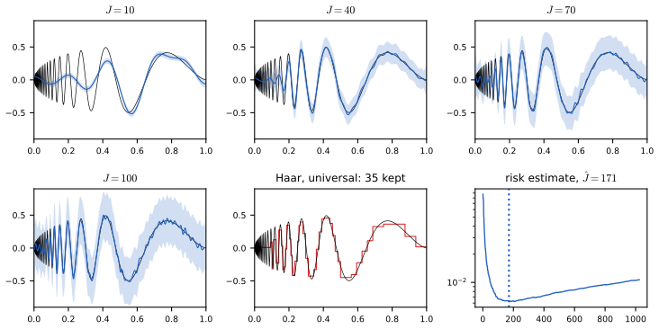
Figure 21.S10 (supplementary). Exercise 21.9: cosine fits and 95% bands for \(J=10,40,70,100\), the Haar fit, and the risk estimate (minimised at \(\hat J=171\)). Not a figure of the book. Code: fig_21_s10. Download: PDF · SVGSolution
(a) As \(J\) grows from 10 to 100, the fit recovers more of the oscillations (at \(J=10\) only those beyond \(x\approx0.4\)) and the band widens roughly in proportion to \(J\). The risk estimate itself would choose \(\hat J=171\). (b) \(\sh=0.115\) and 35 coefficients survive; the step-function fit tracks the oscillations down to \(x\approx0.05\). Demo: preset 3 has the same data, with a \(J\) slider.
Exercise 21.10. Haar density estimation. With \(X_1,\dots,X_n\sim f\) on \([0,1]\), let \(\bh_{j,k}=n^{-1}\sum_i\psi_{j,k}(X_i)\) and define the Haar histogram \(\fh_B=\phi+\sum_{j=0}^B\sum_k\bh_{j,k}\psi_{j,k}\), \(0\le B\le J-1\). (a) Show \(\bh_{j,k}\) is unbiased. (c) Find the MSE as a function of \(B\). (d) For 1000 draws from Beta(15, 4), choose \(B\) by leave-one-out cross-validation.
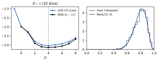
Figure 21.S11 (supplementary). Exercise 21.10: leave-one-out score and exact MSE (shifted by \(\norm f^2\)) against \(B\), and the chosen Haar histogram (\(\hat B=4\), 32 bins). Not a figure of the book. Code: fig_21_s11. Download: PDF · SVGSolution
(a) \(\E\bh_{j,k}=\E\psi_{j,k}(X)=\int\psi_{j,k}f=\beta_{j,k}\). (The coefficient of \(\phi\) is \(\int f=1\), known.)
(b) By Filling the gap 21.13, \(\phi\) and the \(\psi_{j,k}\) with \(j\le B\) span \(V_{B+1}\), and \(\fh_B\) is the empirical version of the projection: on each of the \(m=2^{B+1}\) equal bins it equals \(mN_b/n\), with \(N_b\) the count in bin \(b\). The Haar histogram is the ordinary histogram with \(2^{B+1}\) bins.
(c) As in Theorem 21.5, \[\mathrm{MSE}(B)=\E\norm{\fh_B-f}^2=\sum_{j\le B,k}\V\bh_{j,k}+\sum_{j>B,k}\beta_{j,k}^2\,,\] with \[\V\bh_{j,k}=(\E\psi_{j,k}^2(X)-\beta_{j,k}^2)/n=(2^jP(I_{j,k})-\beta_{j,k}^2)/n\,.\] Since \(\sum_kP(I_{j,k})=1\), \[ \mathrm{MSE}(B)=\frac{2^{B+1}-1-\sum_{j\le B,k}\beta_{j,k}^2}{n}+\sum_{j>B,k}\beta_{j,k}^2 . \]
(d) Leave-one-out cross-validation estimates \(\mathrm{MSE}(B)-\norm f^2\) by \(\int\fh_B^2-\frac2n\sum_i\fh_{B,-i}(X_i)\). For the histogram this is \(\frac m{n^2}\sum_bN_b^2-\frac{2m}{n(n-1)}\sum_bN_b(N_b-1)\), since \(\fh_{B,-i}(X_i)=m(N_b-1)/(n-1)\) for \(X_i\) in bin \(b\) (the shortcut formula for histograms, Theorem 20.7). For 1000 Beta(15, 4) draws it is smallest at \(\hat B=4\) (32 bins), which is also the minimiser of the exact MSE (0.047; computed from the Beta cdf).
Exercise 21.11. The noise estimate (21.37). Let \(X_1,\dots,X_n\sim\N(0,\sigma^2)\) and \(\sh=\med(|X_1|,\dots,|X_n|)/0.6745\). (a) Discuss \(\E\sh=\sigma\). (b) For \(n=100\), compare the MSE of \(\sh\) and of the sample standard deviation over 1000 simulations. (c) Repeat with 5% of the observations drawn from a wider Normal.
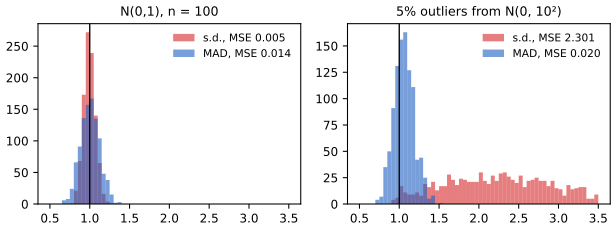
Figure 21.S12 (supplementary). Exercise 21.11: the median-based estimate against the sample standard deviation, without and with 5% outliers from \(\N(0,10^2)\), 1000 samples of size 100. Not a figure of the book. Code: fig_21_s12. Download: PDF · SVGSolution
(a) The book's version has an extra factor \(\sqrt n\) (see the notes on the book). \(|X|\) has median \(\sigma\Phi^{-1}(0.75)=0.6745\sigma\), and the sample median of the \(|X_i|\) converges to it in probability, so \(\sh\to\sigma\); with the density \(2\phi(0.6745)/\sigma=0.636/\sigma\) of \(|X|\) at its median, the sample median is asymptotically Normal with variance \(1/(4n(0.636/\sigma)^2)\), so \(\V\sh\approx1.36\sigma^2/n\). Exact unbiasedness fails: for \(n=100\), \(\E\sh=1.0033\sigma\) (200 000 simulations).
(b) MSE 0.0054 for the standard deviation and 0.0143 for \(\sh\): the median wastes information on clean Normal data (asymptotically \(0.5\sigma^2/n\) against \(1.36\sigma^2/n\)).
(c) Reading the second ".95" as .05 and the wide Normal as standard deviation 10: MSE 2.30 for the standard deviation (it estimates \(\sqrt{0.95+0.05\cdot100}=2.44\)) and 0.020 for \(\sh\). With variance 10 instead: 0.063 and 0.017. This is why (21.37) uses the median: peaks in the signal act like outliers at the finest level.
Exercise 21.12. Repeat Exercise 21.6 with the Haar basis.
Solution
Figure 21.S8, right column, with 4, 16 and 128 terms (all levels below \(B=2,4,7\)); the coefficients are one discrete transform of \(f(r/N)\), \(N=2^{14}\). (a) and (b): smooth functions need many Haar terms; the resolution-\(B\) error falls like \(2^{-B}\) (step functions approximate a slope only to within its rise over one step), much slower than the cosine expansion of (a) (exact) or (b). (c) The blocks function is piecewise constant: at each level only the coefficients whose interval contains a jump are non-zero (at most 11 per level), so it is sparse in the Haar basis and the 128-term sum is almost exact, without ringing. (d) The doppler function needs fine levels only near 0. These are the situations in which wavelets beat a fixed Fourier-type basis.
Demonstrations for this chapter
Each demonstration runs in the browser and links back to these notes. The ▶ Demo boxes above open them already set to the case under discussion.
| Demonstration | What you can see | Sections and results |
|---|---|---|
| Cosine series density estimation | A sample from the Bart Simpson, Beta(15, 4) or Normal density, or the Old Faithful eruption times; the cosine estimate with \(J\) chosen by the risk estimate or by hand; the estimated and true risks; the band of Theorem 21.6 and the corrected band. Presets: 1 Example 21.7; 2 corrected band; 3 \(J=p\); 4 \(n=500\); 5 Old Faithful. | 21.2, Theorems 21.4–21.6 |
| Cosine series regression and its band | Doppler or blocks data with any \(n\) and \(\sigma\), or the glass data; the coefficients against the noise level, the risk estimate and the true risk, and the band of Theorem 21.11 with \(r_J\) and \(r\). Presets: 1 Examples 21.10 and 21.12; 2 \(J=45\); 3 Exercise 21.9; 4 blocks; 5 glass. | 21.3, Theorems 21.8–21.11 |
| The Haar multiresolution ladder | A signal split into its detail layers; resolution-\(J\) estimates against hard or soft thresholding, with the error of each and of the best resolution; pure-noise samples against the universal threshold. Presets: 1–2 Figure 21.7; 3 Example 21.16; 4 best linear resolution; 5 Theorem 21.15. | 21.4, 21.5, Theorems 21.13, 21.15, 21.D |
Related demonstrations in the companion courses: the wavelet shrinkage demo (symmlets, SURE) of Statistical Learning: Theory and Methods, and the histograms, kernel density estimates and nearest neighbours demo of Bayesian and Probabilistic Machine Learning.
References
- Wasserman, L. (2004). All of Statistics: A Concise Course in Statistical Inference. Springer, New York. Chapter 21, pp. 327–348. www.stat.cmu.edu/~larry/all-of-statistics.
- Beran, R. (2000). REACT scatterplot smoothers: superefficiency through basis economy. Journal of the American Statistical Association, 95, 155–171.
- Beran, R. and Dümbgen, L. (1998). Modulation of estimators and confidence sets. The Annals of Statistics, 26, 1826–1856.
- Daubechies, I. (1988). Orthonormal bases of compactly supported wavelets. Communications on Pure and Applied Mathematics, 41, 909–996.
- Donoho, D. L. and Johnstone, I. M. (1994). Ideal spatial adaptation by wavelet shrinkage. Biometrika, 81, 425–455.
- Donoho, D. L. and Johnstone, I. M. (1995). Adapting to unknown smoothness via wavelet shrinkage. Journal of the American Statistical Association, 90, 1200–1224.
- Donoho, D. L. and Johnstone, I. M. (1998). Minimax estimation via wavelet shrinkage. The Annals of Statistics, 26, 879–921.
- Donoho, D. L., Johnstone, I. M., Kerkyacharian, G. and Picard, D. (1995). Wavelet shrinkage: asymptopia? Journal of the Royal Statistical Society, Series B, 57, 301–369.
- Efromovich, S. (1999). Nonparametric Curve Estimation: Methods, Theory and Applications. Springer, New York.
- Härdle, W., Kerkyacharian, G., Picard, D. and Tsybakov, A. (1998). Wavelets, Approximation, and Statistical Applications. Springer, New York.
- Marron, J. S. and Wand, M. P. (1992). Exact mean integrated squared error. The Annals of Statistics, 20, 712–736.
- Ogden, R. T. (1997). Essential Wavelets for Statistical Applications and Data Analysis. Birkhäuser, Boston.
- Rudin, W. (1987). Real and Complex Analysis, 3rd edition. McGraw-Hill, New York.
The numerical statements in the text (the coefficients and errors of the doppler approximations, the Legendre Gram matrix, the smoothness identity, the exact variances and covariances on the grid, the risk formulas against simulation, the eigenvalue of the claw covariance, the coverage of both bands, the transform against the direct sums, the survival probabilities of Theorem 21.15, the closed-form thresholding risks and the oracle bound, and the exercise results) were confirmed numerically with the chapter's code.