Prototype Methods and Nearest-Neighbors
The simplest classifiers of all: store some labelled points and give a new point the class of the nearest ones. Prototype methods store a few well-placed points per class (K-means, learning vector quantisation, Gaussian mixtures); nearest-neighbour rules store the whole training set. They model nothing, explain little and often predict very well. This chapter shows where to put the prototypes, why the 1-nearest-neighbour rule is never worse than twice the Bayes rate in the limit, how to make distances ignore transformations that do not change the class (tangent distance), and how to bend the metric locally so that neighbourhoods follow the class boundary (DANN).
Ch. 1 Introduction Ch. 2 Supervised learning Ch. 3 Linear regression Ch. 4 Linear classification Ch. 5 Basis expansions Ch. 6 Kernel smoothing Ch. 7 Model assessment Ch. 8 Inference and averaging Ch. 9 Additive models and trees Ch. 10 Boosting Ch. 11 Neural networks Ch. 12 SVMs Ch. 13 Nearest neighbours Ch. 14 Unsupervised learning Ch. 15 Random forests Ch. 16 Ensembles Ch. 17 Graphical models Ch. 18 High-dimensional problems
How to read these notes
They follow the book. Sections carry the book's numbers (13.2, 13.2.1, ...) and every displayed equation that appears in the book carries the book's own equation number, e.g. \((13.5)\), so you can read these notes next to the book. Equations without a number are steps that the book skips.
Filling the gaps. Wherever the book says that something "can be shown", leaves it to an exercise, or states a property without proof, an orange Filling the gap box or a proof gives the full argument. Proofs and derivations start hidden: open one with its bar, or use the button below.
Figures and demonstrations. Eleven of the chapter's fifteen figures and Table 13.1 are reproduced from scratch by the Python code; Figures 13.6 and 13.8 need the LANDSAT scene of the STATLOG project, which is not among the book's data sets, and Figures 13.7 and 13.11 are diagrams. Three supplementary figures (13.S1–13.S3) illustrate exercises and the Cover–Hart bound. The ▶ Demo boxes open an interactive demonstration already set to the case being discussed.
Main reference
T. Hastie, R. Tibshirani and J. Friedman, The Elements of Statistical Learning: Data Mining, Inference, and Prediction, 2nd edition, Springer (2009), Chapter 13, pages 459–483 (book website, with the data sets: hastie.su.domains/ElemStatLearn). Section, equation, figure, table and exercise numbers below refer to this book. Further reading is listed in the references.
The explanations, derivations, figures and code are my own; equations are cited by their numbers in the book.
Companion courses
Parts of this chapter also appear in the two companion courses on this site. The overlapping material is:
- Section 13.2.1 (K-means, its two steps and its convergence): Bayesian and Probabilistic Machine Learning, Section 9.1 and Result 9.1; Foundations of Deep Learning, Section 15.1 (K-means and vector quantisation, Result 15.1).
- Section 13.2.2 (on-line updates with decreasing step sizes): the sequential K-means update as a Robbins–Monro step, Filling the gap 9.2, and Filling the gap 15.1.
- Section 13.2.3 and Exercise 13.1 (Gaussian mixtures, EM, and K-means as the small-variance limit of EM): Section 9.2.2, Result 9.9; Foundations of Deep Learning, Section 15.3.2.
- Section 13.3 (nearest-neighbour classification as a density estimate, and the Cover–Hart bound): Bayesian and Probabilistic Machine Learning, Section 2.5.2, Section 2.5.3 and Result 2.28.
Within this course the chapter builds on Section 2.3 (k-NN on the mixture data), Section 2.5 (the curse of dimensionality), Section 4.3 (within- and between-class covariances), Section 7.10 (cross-validation) and Section 12.7 (mixture discriminant analysis, which is the Gaussian mixture classifier of Figure 13.2). New here: the fixed point that explains LVQ, a full proof of the Cover–Hart bound with its convergence step, tangent distance in closed form, the DANN metric derived as a local chi-squared distance between class posteriors, and five notes on the book (the radius of Section 13.4.1, the direction of stretching, pure regions, Exercise 13.5, Exercise 13.8).
The chapter at a glance
- 13.2 A prototype classifier partitions the plane into convex cells with piecewise-linear boundaries (Result 13.2). K-means places prototypes class by class (Result 13.1); LVQ1 (Algorithm 13.1) moves each prototype to the point where attraction by its own class balances repulsion by the others (Result 13.3); Gaussian mixtures are soft prototypes and become K-means as the variance shrinks (Result 13.4).
- 13.3 The k-NN vote estimates the class posterior locally (Result 13.5). As \(N\to\infty\) the 1-NN error tends to \(E_1=\E\sum_kp_k(1-p_k)\) (Result 13.6), which lies between \(E^*\) and \(E^*(2-\frac{K}{K-1}E^*)\) (Result 13.7). Tangent distance makes 1-NN nearly invariant to small transformations at the cost of a small least-squares problem (Result 13.8).
- 13.4 In high dimensions the nearest neighbour is far away (Result 13.9). DANN shrinks the neighbourhood across the local discriminant direction with the metric (13.9) (Result 13.10), which is the first-order chi-squared distance between class posteriors (Result 13.11); averaging the local between-class matrices gives a global subspace (Result 13.12).
- 13.5 Condensing keeps a subset on which 1-NN still classifies every training point correctly (Result 13.13).
Notation. Training data \((x_i,g_i)\), \(i=1,\dots,N\), \(x_i\in\R^p\), \(g_i\in\{1,\dots,K\}\). \(p_k(x)=\Pr(G=k\given X=x)\) are the class posteriors, \(k^*=\argmax_kp_k(x)\) the Bayes class, \(E^*\) the Bayes error rate. Prototypes \(m_j\) with labels \(c_j\); \(R\) prototypes per class. \(\bW\), \(\bB\) are within- and between-class covariance matrices (divisor \(n\)).
Prerequisites. The Bayes classifier (Section 2.4), LDA (Section 4.3), cross-validation (Section 7.10), the EM algorithm (Section 8.5), and Jensen's and the Cauchy–Schwarz inequalities.
13.1 Introduction
p. 459 The methods of this chapter assume almost nothing about how the class depends on the features. That makes them poor tools for understanding the relationship, but strong black-box predictors, often among the best on real problems. Nearest neighbours can also be used for regression (Chapter 2), but there the bias–variance trade-off degrades quickly with the dimension; for classification it is kinder, because only the side of the decision boundary matters, not the value of the posterior (compare Section 7.3.1).
13.2 Prototype Methods
pp. 459–460 The training data are \(N\) pairs \((x_1,g_1),\dots,(x_N,g_N)\) with \(g_i\in\{1,\dots,K\}\). Features are usually standardised to mean 0 and variance 1 first, so that Euclidean distance does not depend on the units.
Definition 13.1 (prototype classifier) pp. 459–460
A prototype classifier is a finite set of points \(m_1,\dots,m_J\in\R^p\) with class labels \(c_1,\dots,c_J\), and the rule
\[ \hat G(x)=c_{\hat\jmath(x)},\qquad \hat\jmath(x)=\argmin_j\|x-m_j\|. \]The 1-nearest-neighbour rule is the special case where the prototypes are all the training points with their own labels. Methods differ in how many prototypes they use and where they put them.
Result 13.2 (the decision regions are unions of convex polyhedra)
Let \(V_j=\{x:\|x-m_j\|\le\|x-m_l\|\ \forall l\}\) be the Voronoi cell of prototype \(j\). Each \(V_j\) is an intersection of half-spaces, hence a convex polyhedron, and the region assigned to class \(k\) is \(\bigcup_{j:c_j=k}V_j\). The decision boundary is piecewise linear: it is made of pieces of the perpendicular bisectors of pairs \(m_j,m_l\) with \(c_j\ne c_l\). Equivalently \(\hat G(x)=\argmax_k\max_{j:c_j=k}\big(2m_j^\T x-\|m_j\|^2\big)\).
Proof
\(\|x-m_j\|^2\le\|x-m_l\|^2\) expands to \(-2m_j^\T x+\|m_j\|^2\le-2m_l^\T x+\|m_l\|^2\), i.e. \(2(m_l-m_j)^\T x\le\|m_l\|^2-\|m_j\|^2\): a closed half-space bounded by the hyperplane through \((m_j+m_l)/2\) orthogonal to \(m_l-m_j\). \(V_j\) is the intersection of these \(J-1\) half-spaces. Minimising \(\|x-m_j\|^2\) over \(j\) is maximising the linear functions \(2m_j^\T x-\|m_j\|^2\), since \(\|x\|^2\) is common to all \(j\). A boundary point between two classes is a point of \(V_j\cap V_l\) with \(c_j\ne c_l\), which lies on the bisector of \(m_j\) and \(m_l\). ∎
13.2.1 K-means Clustering
pp. 460–462 K-means looks for \(R\) centres that minimise the total within-cluster sum of squares. From initial centres (usually \(R\) random training points) it alternates two steps: give each point to its nearest centre; replace each centre by the mean of its points. (The book writes \(R\) for the number of centres because \(K\) is the number of classes.) For classification, run K-means separately on the training points of each class with \(R\) centres each, label the \(KR\) centres by their class, and classify by the nearest centre.
See also (companion courses): Section 9.1, K-means clustering; Foundations of Deep Learning, Section 15.1.
Result 13.1 (K-means decreases the within-cluster sum of squares and stops) p. 460
Let \(J(C,m)=\sum_{i}\|x_i-m_{C(i)}\|^2\) for an assignment \(C\) of the points to \(R\) clusters and centres \(m_1,\dots,m_R\). Neither step of K-means increases \(J\), and the algorithm stops after finitely many iterations at a point where both steps leave \(J\) unchanged.
Proof (sketch; the companion course gives the details)
For fixed centres, assigning each point to its nearest centre minimises each term \(\|x_i-m_{C(i)}\|^2\) separately. For a fixed assignment, \(\sum_{C(i)=r}\|x_i-m\|^2=\sum_{C(i)=r}\|x_i-\bar x_r\|^2+N_r\|\bar x_r-m\|^2\), minimised by the cluster mean. So \(J\) never increases. There are finitely many assignments, the centres are a function of the assignment, and an assignment cannot repeat unless \(J\) has stopped decreasing; with the rule "stop when the assignment does not change" the algorithm terminates. The limit is a local minimum in the sense of these two coordinate blocks, not in general the global minimum, which is why several random starts are used. Full proof: Result 9.1 of the companion course. ∎
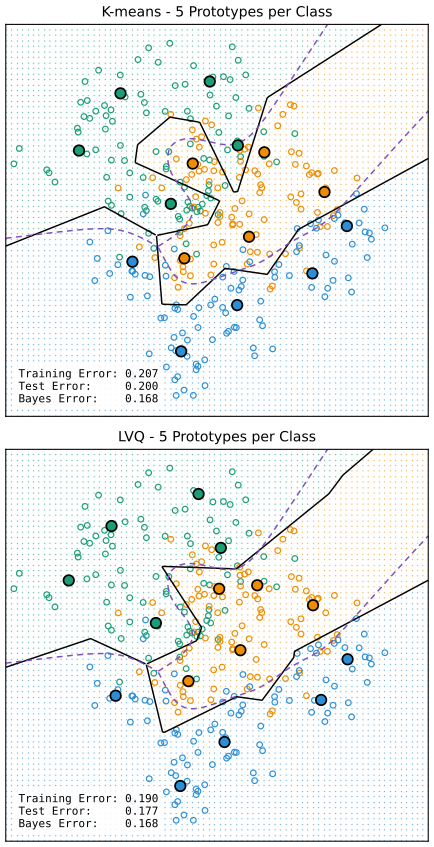
fig_13_1. Reproduces Hastie, Tibshirani and Friedman (2009), Figure 13.1. Download: PDF · SVGThe obvious weakness: each class places its prototypes without looking at the others, so prototypes can land close to the boundary, or even inside another class's territory, and cost errors there.
13.2.2 Learning Vector Quantization
pp. 462–463 Kohonen's (1989) learning vector quantisation uses all the data to place all the prototypes. It is an on-line algorithm.
Algorithm 13.1 (learning vector quantisation, LVQ1; Kohonen, 1989) p. 462
- Choose \(R\) initial prototypes per class, \(m_1(k),\dots,m_R(k)\), \(k=1,\dots,K\), for example \(R\) random training points of each class (or the K-means centres).
- Draw a training point \(x_i\) at random (with replacement) and let \(m_j(k)\) be the prototype closest to it.
- If \(g_i=k\), move the prototype towards the point: \(m_j(k)\leftarrow m_j(k)+\epsilon\,(x_i-m_j(k))\).
- If \(g_i\ne k\), move it away: \(m_j(k)\leftarrow m_j(k)-\epsilon\,(x_i-m_j(k))\).
- Repeat step 2, decreasing the learning rate \(\epsilon\) towards zero.
The code uses \(\epsilon_t=\epsilon_0(1-t/T)\) over \(T\) steps (\(T\) = number of passes times \(N\)). Variants LVQ2 and LVQ3 also move the runner-up prototype.
Filling the gap 13.1: what one step does, and the step sizes p. 462
Derivation
One step. The attracting update gives \(m'-x_i=(1-\epsilon)(m-x_i)\): the prototype moves along the segment towards \(x_i\) and its distance to \(x_i\) shrinks by the factor \(1-\epsilon\). The repelling update gives \(m'-x_i=(1+\epsilon)(m-x_i)\): it moves along the same line away from \(x_i\), and the distance grows by \(1+\epsilon\).
A stochastic gradient, piece by piece. Fix the Voronoi cells \(V_j\) of the current prototypes and let \(s_{ij}=+1\) if \(g_i=c_j\) and \(-1\) otherwise. The signed distortion
\[ \tilde J(m)=\frac1{2N}\sum_j\sum_{x_i\in V_j}s_{ij}\|x_i-m_j\|^2 \]has \(\partial\tilde J/\partial m_j=-\frac1N\sum_{x_i\in V_j}s_{ij}(x_i-m_j)\), and the LVQ1 step is \(m_j\leftarrow m_j+\epsilon s_{ij}(x_i-m_j)\) for a random \(x_i\in V_j\): an unbiased estimate of \(-N\epsilon\,\partial\tilde J/\partial m_j\) divided by \(N\), i.e. one stochastic-gradient step. The cells change as the prototypes move, so LVQ1 descends a different function in each configuration and there is no single criterion it minimises; this is the "defined by an algorithm rather than an optimisation" drawback the book mentions.
Step sizes. For stochastic approximation (Section 11.4; Robbins and Monro, 1951) the steps should satisfy \(\sum_t\epsilon_t=\infty\) (the prototypes can travel any distance) and \(\sum_t\epsilon_t^2\lt\infty\) (the accumulated noise has finite variance), e.g. \(\epsilon_t=\epsilon_0/(1+t/\tau)\). With a fixed budget of \(T\) steps the linear decay to zero used here plays the same role. See also Filling the gap 9.2 of the companion course. ∎
Result 13.3 (where LVQ1 moves a prototype: attraction balanced by repulsion)
Average the LVQ1 step over a random \(x_i\) with the cells held fixed. A prototype \(m_j\) is at rest (in this mean-field sense) iff \(\sum_{x_i\in V_j}s_{ij}(x_i-m_j)=0\). If its cell holds \(n_+\) points of its own class with mean \(\bar x_+\) and \(n_-\lt n_+\) points of other classes with mean \(\bar x_-\), the rest point is
\[ m_j=\frac{n_+\bar x_+-n_-\bar x_-}{n_+-n_-}=\bar x_++\frac{n_-}{n_+-n_-}\,(\bar x_+-\bar x_-). \]So LVQ starts from the K-means position \(\bar x_+\) (when the cell has no intruders) and pushes the prototype from the mean of its own points away from the mean of the intruders, by a factor that grows as the intruders become numerous. If \(n_-\ge n_+\) there is no rest point and the prototype is driven away until its cell changes.
Proof
With \(x_i\) drawn uniformly from the \(N\) points, the expected change of \(m_j\) is \(\frac{\epsilon}{N}\sum_{x_i\in V_j}s_{ij}(x_i-m_j)\), which vanishes iff \(\sum_{V_j}s_{ij}x_i=m_j\sum_{V_j}s_{ij}\), i.e. \(n_+\bar x_+-n_-\bar x_-=(n_+-n_-)m_j\). Divide by \(n_+-n_-\gt0\) and write \(n_+\bar x_+-n_-\bar x_-=(n_+-n_-)\bar x_++n_-(\bar x_+-\bar x_-)\). If \(n_-\ge n_+\) the coefficient of \(m_j\) in the expected step, \(-(n_+-n_-)\epsilon/N\), is non-negative, so the expected step does not shrink deviations from any point: no stable rest point exists. ∎
This explains Figure 13.1: prototypes whose cells straddle the boundary have intruders and are pushed back into their own class. It also explains a failure: with one prototype per class (\(R=1\)) each cell holds many intruders, \(n_-/(n_+-n_-)\) is large, and LVQ throws the centroids apart; on the three-class data the test error rises from 0.254 to 0.274 (demo preset 5).
13.2.3 Gaussian Mixtures
p. 463 A Gaussian mixture is a prototype method in which each prototype is a Gaussian density with a centre and a covariance. EM alternates an E-step, which gives each observation a responsibility for each component in proportion to the component's likelihood, and an M-step, which recomputes the weighted means and covariances. Points near a centre get responsibility close to 1; points between centres share. Hence "soft" clustering, against K-means' hard assignments. Used class by class with a common covariance, this is mixture discriminant analysis (Section 12.7): the posteriors \(\hat p_k(x)\) of (12.60) are smooth, but the classification \(\hat G(x)=\argmax_k\hat p_k(x)\) is as hard as any other.
See also (companion courses): Section 9.2.2, EM for Gaussian mixtures; Foundations of Deep Learning, Section 15.3.2, relation to K-means.
Result 13.4 (scalar-covariance mixtures harden into K-means; Exercise 13.1) p. 463
For a mixture of \(R\) Gaussians with known covariance \(\sigma^2\bI\) and equal weights, the E-step responsibilities are
\[ \gamma_{ir}=\frac{\exp\{-\|x_i-m_r\|^2/(2\sigma^2)\}}{\sum_s\exp\{-\|x_i-m_s\|^2/(2\sigma^2)\}}, \]a softmax of minus the squared distances at temperature \(2\sigma^2\), and the M-step sets \(m_r=\sum_i\gamma_{ir}x_i/\sum_i\gamma_{ir}\). As \(\sigma\to0\), \(\gamma_{ir}\to1\) if \(m_r\) is the unique nearest centre to \(x_i\) and 0 otherwise, so the E-step becomes the K-means assignment and the M-step the K-means mean: the two algorithms coincide. The proof is Exercise 13.1.
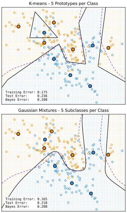
fig_13_2. Reproduces Hastie, Tibshirani and Friedman (2009), Figure 13.2. Download: PDF · SVGAs the book notes, both methods spend a blue prototype in the north-west, where the data are orange-dominated; the mixture can down-weight it through its mixing proportion and its overlap with orange components, while K-means must give it a whole Voronoi cell. LVQ makes little difference on these data (demo preset 3: test error 0.236 for K-means, 0.242 after 20 LVQ passes).
13.3 k-Nearest-Neighbor Classifiers
pp. 463–468 No model is fitted. For a query \(x_0\), find the \(k\) training points \(x_{(r)}\), \(r=1,\dots,k\), closest to \(x_0\) and take a majority vote of their classes (ties at random; the code gives a tie to the tied class whose nearest member comes first). With real features, after standardisation, the distance is
\[ d_{(i)}=\|x_{(i)}-x_0\|. \tag{13.1} \]k-NN has done well on handwritten digits, satellite images and EKG patterns: problems where each class has many prototypes and the boundary is very irregular. In 1-NN every training point is a prototype.
See also (companion course): Section 2.5.2, nearest-neighbour methods (the k-NN classifier from a nearest-neighbour density estimate); in this course, Section 2.3.2.
Result 13.5 (the vote is the arg max of a local posterior estimate)
Let \(N_k(x_0)\) be the set of the \(k\) nearest training points and \(\hat p_j(x_0)=\frac1k\#\{x_i\in N_k(x_0):g_i=j\}\). The majority vote is \(\argmax_j\hat p_j(x_0)\). If \(p_j\) is continuous at \(x_0\), \(x_0\) is in the support of \(X\), and \(k\to\infty\), \(k/N\to0\), then \(\hat p_j(x_0)\to p_j(x_0)\) in probability, so the rule tends to the Bayes rule wherever the Bayes class is unique.
Proof
The first statement is the definition of the vote. For the second: with \(k/N\to0\) the radius of \(N_k(x_0)\) tends to 0 in probability (the ball \(B(x_0,\delta)\) has positive probability \(\mu_\delta\), and the number of training points in it is Binomial\((N,\mu_\delta)\), which exceeds \(k\) with probability tending to 1). Given the neighbours' positions, their labels are independent with probabilities \(p_j(x_{(r)})\), all within \(\eta\) of \(p_j(x_0)\) once the radius is small (continuity). So \(\E\hat p_j\) is within \(\eta\) of \(p_j(x_0)\) and \(\Var\hat p_j\le1/(4k)\to0\); Chebyshev's inequality finishes the argument. The same estimate with \(k=K_kNV\) volumes gives the density-ratio form of the companion course (2.256). ∎
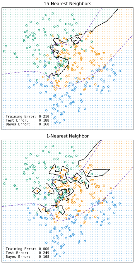
fig_13_3. Reproduces Hastie, Tibshirani and Friedman (2009), Figure 13.3. Download: PDF · SVGFigure 13.4 plots the training, test and ten-fold cross-validation errors against \(k\) for the two-class mixture data. Because the CV error is an average of ten fold errors, it comes with a standard error.
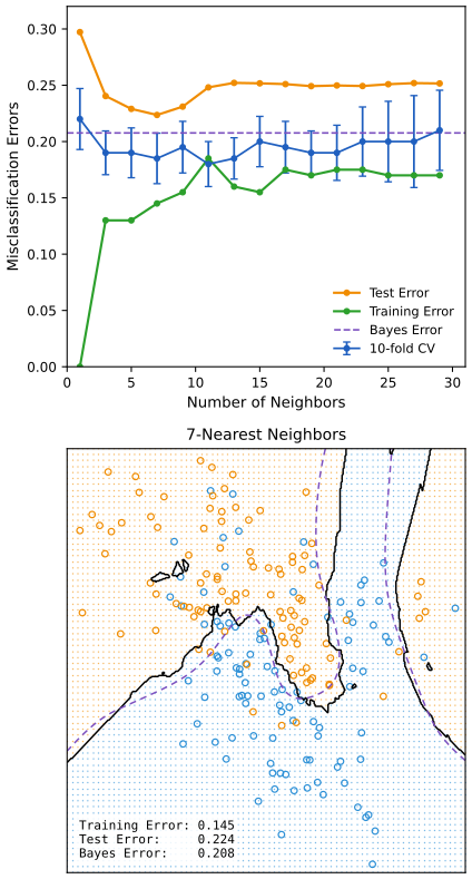
fig_13_4. Reproduces Hastie, Tibshirani and Friedman (2009), Figure 13.4. Download: PDF · SVGFilling the gap 13.2: the standard error of the CV curve p. 465
Derivation
With \(V\) folds, \(\widehat{\rm CV}=\frac1V\sum_{v=1}^Ve_v\) where \(e_v\) is the error on fold \(v\) of the rule trained on the other folds (equal fold sizes). If the \(e_v\) were independent with common variance \(\sigma^2\), \(\Var\widehat{\rm CV}=\sigma^2/V\), estimated by \(s^2/V\) with \(s^2=\frac1{V-1}\sum_v(e_v-\widehat{\rm CV})^2\); the bars in Figure 13.4 are \(\pm s/\sqrt V\). The folds share most of their training data, so the \(e_v\) are positively correlated and the true variance is larger: the bars are optimistic, a reason to prefer the one-standard-error rule over chasing the minimum (Section 7.10). ∎
The Cover–Hart result. 1-NN uses only the closest point, so its bias is small and its variance large. Cover and Hart (1967) showed that asymptotically its error is never more than twice the Bayes rate. The idea: as \(N\to\infty\) the nearest neighbour sits on top of the query point, so 1-NN guesses the class of \(x_0\) with an independent draw from the same posterior.
See also (companion course): Result 2.28, the Cover–Hart bound, with a proof for two classes.
Result 13.6 (the asymptotic 1-NN error) pp. 465–467, (13.2)–(13.4)
At \(x\), with \(k^*\) the dominant class,
\[ \text{Bayes error}=1-p_{k^*}(x), \tag{13.2} \] \[ \text{1-nearest-neighbor error}=\sum_{k=1}^Kp_k(x)\big(1-p_k(x)\big) \tag{13.3} \] \[ \ge\ 1-p_{k^*}(x). \tag{13.4} \]Precisely: suppose \(X\) has distribution \(\mu\) on \(\R^p\), each \(p_k\) is continuous, and the training sample is i.i.d. Then the conditional error of 1-NN at a query \(x\) in the support of \(\mu\) tends to (13.3), and its overall error tends to \(E_1=\E\sum_kp_k(X)(1-p_k(X))\).
Proof
The neighbour converges to the query. Fix \(x\) in the support, so \(\mu(B(x,\delta))\gt0\) for every \(\delta\gt0\). The nearest neighbour \(x_{(1)}\) is farther than \(\delta\) only if no training point falls in \(B(x,\delta)\), which has probability \((1-\mu(B(x,\delta)))^N\to0\). So \(x_{(1)}\to x\) in probability.
The conditional error. Given the training inputs, the query's class \(G\sim p(x)\) and the neighbour's class \(G'\sim p(x_{(1)})\) are independent, and 1-NN errs iff \(G\ne G'\):
\[ \Pr(G\ne G'\given x,x_{(1)})=1-\sum_kp_k(x)p_k(x_{(1)}). \]By continuity this tends to \(1-\sum_kp_k(x)^2=\sum_kp_k(x)(1-p_k(x))\), using \(\sum_kp_k=1\). That is (13.3). Averaging over \(x\) (bounded convergence; the error is in \([0,1]\)) gives \(E_1\).
(13.4). \(\sum_kp_k(1-p_k)\ge\sum_kp_k(1-p_{k^*})=1-p_{k^*}\), since \(p_k\le p_{k^*}\) for every \(k\). Equality holds iff \(p_k(1-p_k)=p_k(1-p_{k^*})\) for all \(k\), i.e. all classes with \(p_k\gt0\) have \(p_k=p_{k^*}\): either one class has probability 1 or the positive ones tie. ∎
The random rule of the book: pick the query's class and the predicted class independently from \(p(x)\); the probability that they differ is (13.3).
Filling the gap 13.3: "twice the variance", with squared-error loss p. 465
Derivation
Two classes, \(Y\in\{0,1\}\), \(p=\Pr(Y=1\given x)\), squared-error loss. The best prediction is \(p\), with risk \(\E(Y-p)^2=\Var Y=p(1-p)\). Asymptotic 1-NN predicts with the neighbour's label \(Y'\), independent of \(Y\) with the same distribution: \(\E(Y-Y')^2=\Var Y+\Var Y'=2p(1-p)\), "one variance for the training target and one for the query target". With 0–1 loss the same independence gives \(\Pr(Y\ne Y')=2p(1-p)\), while the Bayes error is \(\min(p,1-p)\); since \(\max(p,1-p)\le1\), \(2p(1-p)\le2\min(p,1-p)\). ∎
Result 13.7 (the Cover–Hart bound) p. 468, (13.5), and Exercise 13.3, (13.12)
For every probability vector \((p_1,\dots,p_K)\) with largest entry \(p_{k^*}\),
\[ \sum_{k=1}^Kp_k(x)\big(1-p_k(x)\big)\ \le\ 2\big(1-p_{k^*}(x)\big)-\frac{K}{K-1}\big(1-p_{k^*}(x)\big)^2, \tag{13.5} \]with equality iff the \(K-1\) other classes have equal probabilities. Consequently
\[ E^*\ \le\ E_1\ \le\ E^*\Big(2-E^*\frac{K}{K-1}\Big)\ \le\ 2E^*. \tag{13.12} \]For \(K=2\), (13.5) is the identity \(2p_{k^*}(1-p_{k^*})\) and (13.12) reads \(E_1\le2E^*(1-E^*)\).
Proof
(13.5). Write \(e=1-p_{k^*}\), so the other probabilities sum to \(e\). Since \(\sum_kp_k=1\), \(\sum_kp_k(1-p_k)=1-\sum_kp_k^2=1-(1-e)^2-\sum_{k\ne k^*}p_k^2\). By Cauchy–Schwarz, \(e^2=(\sum_{k\ne k^*}p_k\cdot1)^2\le(K-1)\sum_{k\ne k^*}p_k^2\), so
\[ \sum_kp_k(1-p_k)\le1-(1-e)^2-\frac{e^2}{K-1}=2e-e^2-\frac{e^2}{K-1}=2e-\frac{K}{K-1}e^2, \]with equality iff the vector \((p_k)_{k\ne k^*}\) is proportional to \((1,\dots,1)\).
(13.12). Let \(e(X)=1-p_{k^*}(X)\), so \(E^*=\E e(X)\). The function \(\varphi(e)=2e-\frac{K}{K-1}e^2\) is concave. Taking expectations in (13.5) and applying Jensen's inequality, \(E_1\le\E\varphi(e(X))\le\varphi(\E e(X))=\varphi(E^*)\). The lower bound is (13.4) averaged. Finally \(\varphi(E^*)\le2E^*\). ∎
Two gaps sit between \(E_1\) and the bound: the pointwise one (losing classes need not tie; it vanishes for \(K=2\)) and Jensen's (the bound is tight only if \(e(X)\) is constant). On the spiral problem of the demo with \(\beta=6\): \(E^*=0.066\), \(E_1=0.095\), bound 0.123.
Filling the gap 13.4: what a 10% 1-NN error says about the Bayes rate p. 468
Derivation
From \(E_1\le2E^*\) a 1-NN error of 0.10 gives \(E^*\ge0.05\), the book's statement. Two classes allow more: \(E_1\le2E^*(1-E^*)\) and \(E^*\le\frac12\) give \(E^*\ge\frac12\big(1-\sqrt{1-2E_1}\big)=0.0528\) (solve the quadratic and keep the root below \(\frac12\)). Both statements are about the asymptotic error; a finite-sample 1-NN error includes bias (from neighbours that are not at the query) and is usually larger than \(E_1\), so the inferred lower bound is optimistic about how small \(E^*\) can be. In the demo with \(\beta=20\) and \(N=2000\), 1-NN has error 0.039, above \(E_1=0.029\) and even above the bound 0.039. ∎
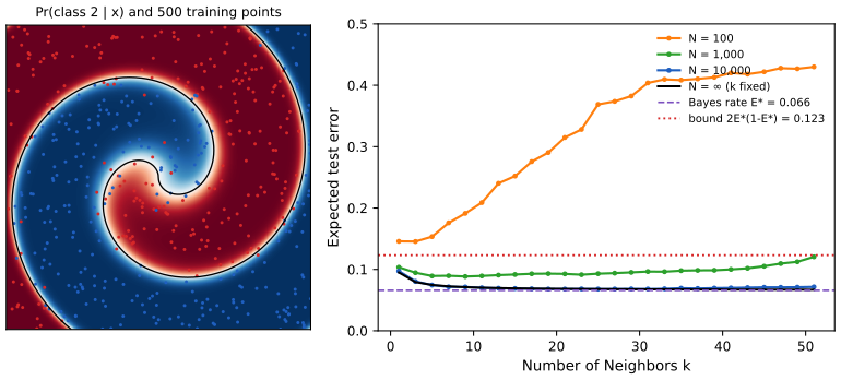
fig_13_s3. Download: PDF · SVG13.3.1 Example: A Comparative Study
pp. 468–470 Ten independent features \(X_j\sim U(0,1)\) and a 0–1 target
\[ Y=I\Big(X_1\gt\tfrac12\Big)\ \ \text{(problem 1, "easy")};\qquad Y=I\Big(\sgn\Big\{\prod_{j=1}^3\big(X_j-\tfrac12\big)\Big\}\gt0\Big)\ \ \text{(problem 2, "difficult")}. \tag{13.6} \]The easy classes are separated by the hyperplane \(X_1=\frac12\); the difficult ones form a checkerboard in the cube of the first three features. Both Bayes rates are 0. There are 100 training and 1000 test observations, and ten realisations.
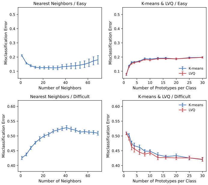
fig_13_5. Reproduces Hastie, Tibshirani and Friedman (2009), Figure 13.5. Download: PDF · SVGFilling the gap 13.5: why one prototype per class is perfect for one problem and useless for the other p. 468
Derivation
Easy. Given \(Y=1\), \(X_1\sim U(\frac12,1)\) and the other features are \(U(0,1)\), independent of \(Y\). The class centroids are \(\mu_1=(\frac34,\frac12,\dots,\frac12)\) and \(\mu_0=(\frac14,\frac12,\dots,\frac12)\). The nearest-centroid rule chooses class 1 iff \(\|x-\mu_1\|^2\lt\|x-\mu_0\|^2\), i.e. \(2(\mu_1-\mu_0)^\T x\gt\|\mu_1\|^2-\|\mu_0\|^2\), i.e. \(x_1\gt\frac12\): the Bayes rule. With estimated centroids the boundary is a slightly tilted hyperplane, hence the small error 0.078; more prototypes per class only add variance. k-NN, in contrast, must find neighbours in all ten dimensions, nine of which are noise, so it needs large \(k\) to average the noise away.
Difficult. The map \(x_1\mapsto1-x_1\) preserves the uniform distribution and flips the sign of the product, so it swaps the classes. Hence the class-conditional distribution of \((X_2,\dots,X_{10})\) is the same in both classes, and the class-1 distribution of \(X_1\) is the class-0 distribution of \(1-X_1\); since given \(X_2,X_3\) the class-1 values of \(X_1\) are \(U(0,\frac12)\) or \(U(\frac12,1)\) with probability \(\frac12\) each (the sign of \((X_2-\frac12)(X_3-\frac12)\) is symmetric), both classes have \(\E X_1=\frac12\). So the two centroids coincide and one prototype per class is a coin toss (error 0.509 in Figure 13.5). Only many local prototypes, or small neighbourhoods, can see the checkerboard, and the six noise dimensions make every neighbourhood large, so the best error stays near 0.42. ∎
The best tuning parameter depends on the problem, and in opposite directions here: it has to be chosen from the data, for instance by cross-validation (Exercise 13.7).
13.3.2 Example: k-Nearest-Neighbors and Image Scene Classification
pp. 470–471 The STATLOG project (Michie et al., 1994) used part of a LANDSAT image (82 × 100 pixels) of agricultural land in Australia, in four spectral bands (two visible, two infrared), with a land-use label per pixel from seven classes (red soil, cotton, vegetation stubble, mixture, grey soil, damp grey soil, very damp grey soil). Each pixel was described by its own four values and those of its eight neighbours (Figure 13.7: the pixel X and its neighbours N), \(9\times4=36\) features, and classified by 5-NN in \(\R^{36}\). The test error was about 9.5%, the best of all methods in the project (LVQ, CART, neural networks, LDA and others; Figure 13.8), and DANN (Section 13.4) did slightly better. Figures 13.6–13.8 are not reproduced: the LANDSAT scene is not among the book's data sets, and Figure 13.8 plots published results.
The success of k-NN suggests that the class boundaries in \(\R^{36}\) are very irregular, and that the neighbourhood features let the rule use spatial smoothness: neighbouring pixels usually share a class.
13.3.3 Invariant Metrics and Tangent Distance
pp. 471–475 In some problems the class does not change under natural transformations of the input. Handwritten digits (16 × 16 grey images, \(\R^{256}\); Figure 13.9) keep their class under small rotations, but a rotated "3" can be far from the original in Euclidean distance.
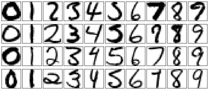
fig_13_9. Reproduces Hastie, Tibshirani and Friedman (2009), Figure 13.9. Download: PDF · SVGDefinition 13.2 (invariance manifold, invariant metric, tangent line) pp. 471–473
Let \(T(x,\alpha)\) be the image \(x\) transformed with parameter \(\alpha\in\R^q\) (rotation angle, shifts, ...), \(T(x,0)=x\). The invariance manifold of \(x\) is \(\mathcal M_x=\{T(x,\alpha)\}\), a \(q\)-dimensional surface in \(\R^{256}\) (a curve for rotation alone). The invariant metric is the distance between manifolds, \(\min_{\alpha,\beta}\|T(x,\alpha)-T(y,\beta)\|\). Its first-order approximation replaces each manifold by its tangent plane at the image,
\[ T(x,\alpha)\approx x+\bT_x\alpha,\qquad \bT_x=\Big[\frac{\partial T(x,\alpha)}{\partial\alpha_1},\dots,\frac{\partial T(x,\alpha)}{\partial\alpha_q}\Big]_{\alpha=0}\in\R^{256\times q}, \]and the (two-sided) tangent distance is \(d_T(x,y)^2=\min_{\alpha,\beta}\|x+\bT_x\alpha-y-\bT_y\beta\|^2\); the one-sided version uses only \(y\)'s tangent plane.
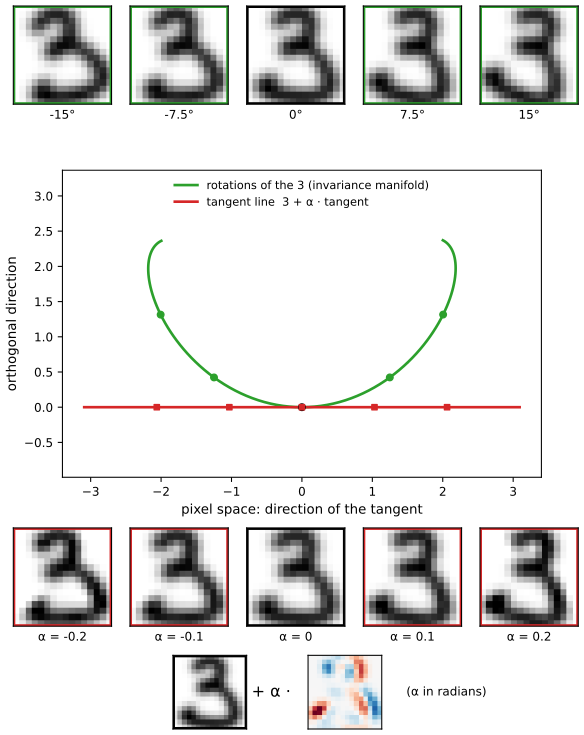
fig_13_10. Reproduces Hastie, Tibshirani and Friedman (2009), Figure 13.10. Download: PDF · SVGThe full invariant metric is hard to compute and allows too much: a "6" rotated by \(180^\circ\) is a "9". The tangent line is cheap and, because it is only first order, large transformations leave the digit's shape behind (the tangent image at large \(\alpha\) no longer looks like a 3). Figure 13.11 of the book sketches two images, their curves and their tangent lines; in \(\R^{256}\) two tangent lines (or seven-dimensional planes) almost surely do not meet, unlike in the drawing.
Result 13.8 (tangent distance in closed form) pp. 473–474
Let \(\bA=[\bT_x,\ -\bT_y]\) have full column rank and \(d=x-y\). Then
\[ d_T(x,y)^2=\|(\bI-\bP_{\bA})d\|^2=d^\T d-d^\T\bA(\bA^\T\bA)^{-1}\bA^\T d, \]the squared distance from \(d\) to the column space of \(\bA\). It satisfies \(d_T(x,y)=d_T(y,x)\le\) one-sided distance \(\le\|x-y\|\), and is invariant to first order: \(d_T(x+\bT_x\gamma,y)=d_T(x,y)\). It is not a metric: distinct images on one tangent line are at distance 0, and the triangle inequality can fail.
Proof
\(x+\bT_x\alpha-y-\bT_y\beta=d+\bA(\alpha;\beta)\), so the minimisation is a least-squares regression of \(-d\) on the columns of \(\bA\); the normal equations give \((\alpha;\beta)=-(\bA^\T\bA)^{-1}\bA^\T d\) and the residual sum of squares is \(\|(\bI-\bP_{\bA})d\|^2\) with \(\bP_{\bA}=\bA(\bA^\T\bA)^{-1}\bA^\T\). Swapping \(x\) and \(y\) changes \(d\) to \(-d\) and \(\bA\) to \(-[\bT_y,-\bT_x]\), the same column space: symmetric. The one-sided problem fixes \(\alpha=0\) and Euclidean distance fixes both at 0; minimising over more variables cannot increase the minimum. Replacing \(x\) by \(x+\bT_x\gamma\) adds \(\bT_x\gamma\in\) col\((\bA)\) to \(d\), which the projection removes (the tangents of the moved image are those of \(x\) to first order). If \(y=x+\bT_x\gamma\) with \(\gamma\ne0\), \(d_T=0\) although \(x\ne y\). ∎
In practice \(\bA^\T\bA\) is \(14\times14\) for seven transformations, so each distance costs a small linear solve on top of the inner products; a penalty \(\lambda\|(\alpha;\beta)\|^2\) can limit the size of the transformations (Simard et al., 1993).
Computing the tangents. They can be estimated from slightly transformed images, or obtained exactly from a smooth version of the image by the chain rule (Exercise 13.4). The code smooths each image with a Gaussian kernel, \(F(u)=\sum_q\phi_h(u-u_q)I_q\), and uses the seven tangents of Simard et al.: \(F_x\), \(F_y\) (translations), \(yF_x-xF_y\) (rotation), \(xF_x+yF_y\) (scaling), \(xF_x-yF_y\) and \(yF_x+xF_y\) (the two hyperbolic deformations; the book's "scaling in two directions" and "shear") and \(F_x^2+F_y^2\) (line thickness), where \((x,y)\) are pixel coordinates about the image centre. A simpler route to invariance is to add transformed copies of the training images ("hints", Abu-Mostafa 1995), which works when the transformation group is small.
| Method | Book | Here |
|---|---|---|
| Neural net | 0.049 | (see Chapter 11) |
| 1-NN, Euclidean distance | 0.055 | 0.0563 |
| 1-NN, Euclidean distance on the smoothed images | 0.0533 | |
| 1-NN, one-sided tangent distance (7 tangents) | 0.0369 | |
| 1-NN, two-sided tangent distance (translations and rotation only) | 0.0399 | |
| 1-NN, two-sided tangent distance (7 tangents) | 0.026 | 0.0289 |
The tangent distance is computed for each test digit against its 100 nearest training digits in Euclidean distance, since it can only be smaller (Result 13.8); on 400 training digits the restriction made no difference. The remaining gap to 0.026 is plausibly the smoothing and the absence of a penalty on the transformations. Tangent-distance 1-NN halves the error of Euclidean 1-NN; as the book says, nearest neighbours were too slow on line, and neural networks were later trained to mimic them.
13.4 Adaptive Nearest-Neighbor Methods
pp. 475–478 In high dimensions the nearest neighbours of a point can be far away, which biases the rule. For \(N\) points uniform in the cube \([-\frac12,\frac12]^p\), let \(R\) be the distance from the origin to the nearest one; with \(v_pr^p\) the volume of the ball of radius \(r\) in \(\R^p\),
\[ \median(R)=v_p^{-1/p}\Big(1-\frac12^{1/N}\Big)^{1/p}. \tag{13.7} \]See also (this course): Section 2.5, the same calculation for the unit ball, and the curse of dimensionality demo.
Result 13.9 (the median nearest-neighbour radius; Exercise 13.2) p. 475, (13.7)
(13.7) holds exactly whenever its right side is at most \(\frac12\), with \(v_p=\pi^{p/2}/\Gamma(\frac p2+1)\). When it exceeds \(\frac12\) the ball leaves the cube and the true median is somewhat larger.
Proof
The points are independent and uniform on a cube of volume 1, so for \(r\le\frac12\) (the ball \(B(0,r)\) lies inside the cube) \(\Pr(\|X_i\|\le r)=\text{vol}\,B(0,r)=v_pr^p\). The nearest point is farther than \(r\) iff all \(N\) points are: \(\Pr(R\gt r)=(1-v_pr^p)^N\). This is continuous and decreasing in \(r\), so the median solves \((1-v_pr^p)^N=\frac12\), i.e. \(v_pr^p=1-2^{-1/N}\), which is (13.7). The volume of the unit ball: integrating the Gaussian density, \(1=\int(2\pi)^{-p/2}e^{-\|x\|^2/2}dx=(2\pi)^{-p/2}\int_0^\infty e^{-r^2/2}\,pv_pr^{p-1}dr=(2\pi)^{-p/2}pv_p2^{p/2-1}\Gamma(p/2)\), so \(v_p=\pi^{p/2}/(\frac p2\Gamma(\frac p2))=\pi^{p/2}/\Gamma(\frac p2+1)\). For \(r\gt\frac12\), \(\Pr(\|X_i\|\le r)=\text{vol}(B(0,r)\cap\text{cube})\lt v_pr^p\), so \(\Pr(R\gt r)\) is larger and the true median exceeds (13.7). ∎
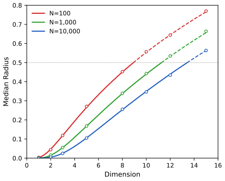
fig_13_12. Reproduces Hastie, Tibshirani and Friedman (2009), Figure 13.12. Download: PDF · SVGNearest-neighbour classification assumes that the class probabilities are roughly constant in the neighbourhood. In Figure 13.13 they change only horizontally: a neighbourhood stretched vertically has the same number of points, lower bias and the same variance. So the metric should be adapted, stretching neighbourhoods in the directions in which the class probabilities do not change; in high dimensions they may change only in a low-dimensional subspace.
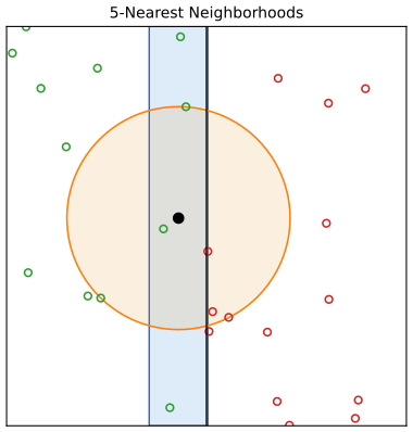
fig_13_13. Reproduces Hastie, Tibshirani and Friedman (2009), Figure 13.13. Download: PDF · SVGp. 477 Friedman (1994a) carves rectangular neighbourhoods adaptively; earlier ideas are in Short and Fukunaga (1981) and Myles and Hand (1990). The discriminant adaptive nearest-neighbour (DANN) rule of Hastie and Tibshirani (1996a) forms a neighbourhood of, say, 50 points at the query, uses its class composition to deform the metric, and then classifies with a nearest-neighbour rule in that metric; every query gets its own metric. The DANN metric at \(x_0\) is
\[ D(x,x_0)=(x-x_0)^\T\bSig(x-x_0), \tag{13.8} \] \[ \bSig=\bW^{-1/2}\big[\bW^{-1/2}\bB\bW^{-1/2}+\epsilon\bI\big]\bW^{-1/2}=\bW^{-1/2}\big[\Bs+\epsilon\bI\big]\bW^{-1/2}, \tag{13.9} \]with \(\bW=\sum_k\pi_k\bW_k\) the pooled within-class covariance and \(\bB=\sum_k\pi_k(\bar x_k-\bar x)(\bar x_k-\bar x)^\T\) the between-class covariance of the 50 neighbours (\(\pi_k\) their class proportions). \(\epsilon=1\) works well in general.
Result 13.10 (what the metric does: sphere, then stretch) p. 477
(13.9) equals \(\bSig=\bW^{-1}\bB\bW^{-1}+\epsilon\bW^{-1}\). In the sphered coordinates \(z=\bW^{-1/2}(x-x_0)\), \(D=z^\T(\Bs+\epsilon\bI)z=\sum_\ell(\theta_\ell+\epsilon)(u_\ell^\T z)^2\), with \(\Bs=\sum_\ell\theta_\ell u_\ell u_\ell^\T\). Directions with \(\theta_\ell=0\), where the local class means do not differ, cost only \(\epsilon\) per unit; the discriminant directions cost \(\theta_\ell+\epsilon\). The neighbourhood \(\{D\le r^2\}\) is an ellipsoid with semi-axes \(r/\sqrt{\theta_\ell+\epsilon}\) along \(u_\ell\) (sphered scale): long where the means agree. With \(\epsilon=0\) it is an infinite slab; with \(\bB=0\) (one class only) \(\bSig=\epsilon\bW^{-1}\).
Proof
Expand: \(\bW^{-1/2}\bW^{-1/2}\bB\bW^{-1/2}\bW^{-1/2}+\epsilon\bW^{-1/2}\bW^{-1/2}=\bW^{-1}\bB\bW^{-1}+\epsilon\bW^{-1}\). For the second form, \((x-x_0)^\T\bW^{-1/2}(\Bs+\epsilon\bI)\bW^{-1/2}(x-x_0)=z^\T(\Bs+\epsilon\bI)z\), and the spectral decomposition of the symmetric positive semidefinite \(\Bs\) gives the sum. With \(K\) classes \(\rank\bB\le K-1\) (the centred means satisfy \(\sum_k\pi_k(\bar x_k-\bar x)=0\)), so for two classes only one direction is penalised. ∎
Result 13.11 (DANN as a local chi-squared distance between class posteriors) p. 477; Hastie and Tibshirani (1996a)
Suppose that near \(x_0\) the classes follow an LDA model: Gaussian with means \(\mu_k\), common covariance \(\bW\) and priors \(\pi_k\). Then, as \(x\to x_0\),
\[ \sum_{k=1}^K\frac{\big[p_k(x)-p_k(x_0)\big]^2}{p_k(x_0)}=(x-x_0)^\T\bW^{-1}\bB(x_0)\bW^{-1}(x-x_0)+o(\|x-x_0\|^2), \]with \(\bB(x_0)=\sum_kp_k(x_0)(\mu_k-\bar\mu)(\mu_k-\bar\mu)^\T\), \(\bar\mu=\sum_kp_k(x_0)\mu_k\). The neighbourhood estimates of (13.9) replace \(p_k(x_0)\) by the class proportions among the 50 neighbours, \(\mu_k\) by the class means and \(\bW\) by the pooled covariance: DANN without \(\epsilon\) measures how much the class posteriors change between \(x_0\) and \(x\), and \(\epsilon\) rounds the resulting slab.
Proof
Under the LDA model \(p_k(x)=\pi_ke^{\delta_k(x)}/\sum_l\pi_le^{\delta_l(x)}\) with \(\delta_k(x)=x^\T\bW^{-1}\mu_k-\frac12\mu_k^\T\bW^{-1}\mu_k\) (Section 4.3), so \(\nabla\delta_k=\bW^{-1}\mu_k\) and, by the quotient rule,
\[ \nabla p_k(x)=p_k(x)\Big[\bW^{-1}\mu_k-\sum_lp_l(x)\bW^{-1}\mu_l\Big]=p_k(x)\,\bW^{-1}\big(\mu_k-\bar\mu(x)\big). \]A first-order Taylor expansion gives \(p_k(x)-p_k(x_0)=p_k(x_0)\,(x-x_0)^\T\bW^{-1}(\mu_k-\bar\mu)+O(\|x-x_0\|^2)\). Square, divide by \(p_k(x_0)\) and sum:
\[ \sum_k\frac{[p_k(x)-p_k(x_0)]^2}{p_k(x_0)}=\sum_kp_k(x_0)\big[(x-x_0)^\T\bW^{-1}(\mu_k-\bar\mu)\big]^2+O(\|x-x_0\|^3)=(x-x_0)^\T\bW^{-1}\bB(x_0)\bW^{-1}(x-x_0)+O(\|x-x_0\|^3). \]Checked numerically on a three-class LDA model: for displacements of size \(10^{-4}\) the ratio of the two sides is 1 to within \(10^{-3}\). ∎
So the null directions of \(\bW^{-1}\bB\bW^{-1}\) are those in which no posterior changes to first order: the directions along the local decision boundary. In Figure 13.13 that is the vertical direction. In general it is not orthogonal to the line joining the class centroids: with a non-spherical \(\bW\) the discriminant direction is \(\bW^{-1}(\mu_2-\mu_1)\), not \(\mu_2-\mu_1\) (compare Figure 4.9).
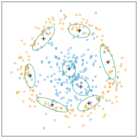
fig_13_14. Reproduces Hastie, Tibshirani and Friedman (2009), Figure 13.14. Download: PDF · SVGNote on the book: the neighbourhoods stretch along the boundary
The book says that in Figure 13.14 "the neighborhoods stretch out orthogonally to the decision boundaries". The figure (the book's and ours) shows the opposite: the ellipses lie along the circular boundary, i.e. orthogonally to the discriminant direction, as the text before (13.8) and Result 13.11 say. At the query at angle \(10^\circ\) on the ring, the long axis of our DANN ellipse is within a few degrees of the tangent to the circle.
Note on the book: in pure regions \(\bSig=\epsilon\bW^{-1}\), not the identity
In a region with one class only, \(\bB=0\) and (13.9) gives \(\bSig=\epsilon\bW^{-1}\) (Result 13.10): a Mahalanobis ball for the local covariance. It is round (as the book says, "the identity", up to the irrelevant factor \(\epsilon\)) only when the 50 neighbours have a nearly isotropic covariance, as at the centre of Figure 13.14.
13.4.1 Example
pp. 478–479 Two classes in ten dimensions, the analogue of Figure 13.14: class 1 has ten independent standard normal features conditioned on the squared radius lying between 22.4 and 40, class 2 is standard normal, 250 points each. Class 1 almost surrounds class 2. There are no noise variables: the discriminating direction changes across the space (it is radial), and every variable matters somewhere. LVQ uses 50 prototypes per class to match 5-NN (\(250/5=50\)).
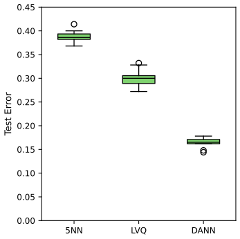
fig_13_15. Reproduces Hastie, Tibshirani and Friedman (2009), Figure 13.15. Download: PDF · SVGNote on the book: "radius" means squared radius
The book conditions on "the radius being greater than 22.4 and less than 40". The radius \(\|X\|\) of a ten-dimensional standard normal is about 3.1 (\(\|X\|^2\sim\chi^2_{10}\)), and \(\Pr(\|X\|\gt22.4)=\Pr(\chi^2_{10}\gt502)\) is zero in double precision, so the condition must be on the squared radius: \(\Pr(\chi^2_{10}\gt22.4)=0.013\), a thin outer shell, which matches the description "the first class almost completely surrounds the second". The code uses \(22.4\lt\|x\|^2\lt40\).
Why plain 5-NN struggles: a shell point has \(\|x\|^2\approx27\) and a central point \(\approx10\). Two shell points in random directions are about \(\sqrt{27+27}\approx7.3\) apart, but a shell point and a central point only about \(\sqrt{27+10}\approx6.1\): the nearest neighbours of shell points are mostly central points. DANN measures distance mainly across the radial direction, where the classes differ, and lets neighbourhoods extend tangentially.
13.4.2 Global Dimension Reduction for Nearest-Neighbors
pp. 479–480 DANN reduces dimension locally. Sometimes a global subspace helps: two nested spheres in four dimensions with six noise features call for 1-NN in the four-dimensional subspace. Hastie and Tibshirani (1996a) compute the between-centroids matrix \(\bB_i\) of the neighbourhood of each training point and average:
\[ \Bbar=\frac1N\sum_{i=1}^N\bB_i. \tag{13.10} \]With eigenvectors \(e_1,\dots,e_p\) of \(\Bbar\) in decreasing order of the eigenvalues \(\theta_\ell\), the leading ones span the best subspaces, because \(\Bbar_{[L]}=\sum_{\ell=1}^L\theta_\ell e_\ell e_\ell^\T\) solves
\[ \min_{\rank(\bM)=L}\ \sum_{i=1}^N\Tr\big[(\bB_i-\bM)^2\big]. \tag{13.11} \]Result 13.12 (the best rank-\(L\) summary of the local between-class matrices; Exercise 13.5) pp. 479–480, (13.10)–(13.11)
Over symmetric \(\bM\) of rank at most \(L\), (13.11) is minimised by \(\Bbar_{[L]}\). Equivalently, the projection \(\bP\) onto \(\span(e_1,\dots,e_L)\) maximises \(\sum_i\Tr(\bP\bB_i)\) among rank-\(L\) orthogonal projections. Writing \(\bB_i=\sum_jb_{ij}u_{ij}u_{ij}^\T\), \(\Tr(\bP\bB_i)=\sum_jb_{ij}\|\bP u_{ij}\|^2\): the subspace captures the local discriminant directions \(u_{ij}\), each weighted by its strength \(b_{ij}\), as fully as possible: a weighted least-squares fit of one subspace to \(N\) subspaces.
Proof
For symmetric matrices \(\Tr(\bA^2)=\|\bA\|_F^2\). Expand around \(\Bbar\): \(\sum_i\|\bB_i-\bM\|_F^2=\sum_i\|\bB_i-\Bbar\|_F^2+N\|\Bbar-\bM\|_F^2+2\sum_i\langle\bB_i-\Bbar,\Bbar-\bM\rangle_F\), and the cross term vanishes because \(\sum_i(\bB_i-\Bbar)=0\). So we must find the best rank-\(L\) approximation of \(\Bbar\) in the Frobenius norm. By the Eckart–Young theorem (proved for symmetric matrices with Weyl's inequalities, or from the SVD) it is the truncated spectral decomposition keeping the \(L\) eigenvalues of largest absolute value; \(\Bbar\) is positive semidefinite (an average of such matrices), so these are the \(L\) largest. For the projection form: for \(\bM=\bP\Bbar\bP\)-type candidates, \(\|\Bbar-\bP\Bbar\bP\|_F^2=\|\Bbar\|_F^2-\|\bP\Bbar\bP\|_F^2\) and Ky Fan's maximum principle gives \(\max_{\bP}\Tr(\bP\Bbar)=\theta_1+\dots+\theta_L\), attained at \(\span(e_1,\dots,e_L)\); and \(\Tr(\bP\Bbar)=\frac1N\sum_i\Tr(\bP\bB_i)\). ∎
On the nested-spheres example (\(N(0,\bI_4)\) against the shell \(9\le\|x\|^2\le16\) of Chapter 12, six noise features, 250 points per class) the eigenvalues of \(\Bbar\) are 0.141, 0.123, 0.095, 0.073, then 0.017 and below; the leading four eigenvectors lie in the signal subspace (squared canonical cosines 0.96 to 0.99). 5-NN has test error 0.252 in all ten dimensions, 0.140 in the estimated four-dimensional subspace and 0.128 in the true one. In the satellite example, the DANN entry of Figure 13.8 used 5-NN in a globally reduced subspace. Duan and Li's (1991) sliced inverse regression finds subspaces by global computations for regression, assuming a spherically symmetric feature distribution.
13.5 Computational Considerations
pp. 480–481 Nearest neighbours cost storage of the whole training set and \(Np\) operations per query. Fast search structures (Friedman et al., 1975, 1977; k-d trees) reduce the search, and Hastie and Simard (1998) built K-means analogues for tangent distance. Storage is reduced by editing and condensing: keep a subset that suffices for nearest-neighbour prediction, ideally the points near the boundary on the correct side.
- Multi-edit (Devijver and Kittler, 1982): split the data at random into several parts, classify each part by 1-NN on the next one (cyclically), delete the misclassified points, and repeat until nothing is deleted for a few rounds. It removes points on the wrong side of the Bayes boundary and leaves homogeneous clusters.
- Condensing (Hart, 1968): start from one random point; pass through the data, adding a point to the store whenever 1-NN on the store misclassifies it; repeat passes until a pass adds nothing. It keeps mainly exterior points of the clusters, near the boundary.
Result 13.13 (condensing terminates with a consistent subset)
If no two training points share an input with different labels, Hart's procedure stops after at most \(N\) additions, and 1-NN on the final store classifies every training point correctly.
Proof
Each pass that does not stop adds at least one new point, and there are \(N\) points, so there are at most \(N\) productive passes. The final pass adds nothing: every point not in the store is classified correctly by 1-NN on the store. A point in the store is its own nearest neighbour (distance 0), and no other stored point has the same input with another label, so it is classified correctly too. ∎
Consistency on the training set says nothing about test error: condensing alone keeps the noisy points near the boundary.
On the mixture data, 1-NN with all 200 points has test error 0.297. Multi-edit (three parts) keeps 117 points (error 0.255); condensing those keeps 7 points with error 0.247, better than all 200. Condensing the raw data keeps 92 points but has error 0.311, since it faithfully keeps the noise. The book reports little practical experience with these methods; the order (edit first, then condense) matters.
Exercises
All 8 exercises of Chapter 13 (Hastie, Tibshirani and Friedman, 2009, pp. 481–483), restated in my own words, with complete solutions (hidden).
Exercise 13.1. In a Gaussian mixture with scalar covariances \(\bSig_r=\sigma\bI\) for all \(r\), \(\sigma\) fixed, discuss the analogy between K-means and EM in detail, and show that the two coincide as \(\sigma\to0\).
Solution
Write the component variance as \(\sigma^2\) (the book's \(\sigma\bI\) is a variance; nothing changes) and take mixing weights \(\pi_r\gt0\). E-step: \(\gamma_{ir}=\pi_r\exp(-\|x_i-m_r\|^2/2\sigma^2)/\sum_s\pi_s\exp(-\|x_i-m_s\|^2/2\sigma^2)\). M-step: \(m_r=\sum_i\gamma_{ir}x_i/\sum_i\gamma_{ir}\), \(\pi_r=\frac1N\sum_i\gamma_{ir}\). The analogy: the E-step is a soft version of "assign each point to its nearest centre" (weights instead of 0/1), and the M-step is the weighted version of "replace each centre by the mean of its points". EM maximises the likelihood, K-means minimises \(\sum_i\min_r\|x_i-m_r\|^2\); the expected complete-data log-likelihood is \(-\frac1{2\sigma^2}\sum_i\sum_r\gamma_{ir}\|x_i-m_r\|^2+\) terms free of the means, a soft within-cluster sum of squares.
The limit. Fix the centres and a point \(x_i\) whose nearest centre \(m_{r^*}\) is unique, with gap \(\Delta=\min_{s\ne r^*}\|x_i-m_s\|^2-\|x_i-m_{r^*}\|^2\gt0\). Dividing numerator and denominator by the \(r^*\) term,
\[ \gamma_{ir}=\frac{(\pi_r/\pi_{r^*})e^{-(\|x_i-m_r\|^2-\|x_i-m_{r^*}\|^2)/2\sigma^2}}{1+\sum_{s\ne r^*}(\pi_s/\pi_{r^*})e^{-(\|x_i-m_s\|^2-\|x_i-m_{r^*}\|^2)/2\sigma^2}}, \]and each exponent with \(r\ne r^*\) is at most \(-\Delta/2\sigma^2\to-\infty\). So \(\gamma_{ir}\to1\) for \(r=r^*\) and 0 otherwise, whatever the \(\pi\)'s: the E-step becomes the K-means assignment, and the M-step the cluster mean. Hence for any fixed number of iterations from a common start, EM's centres converge to K-means' as \(\sigma\to0\) (the maps are continuous at configurations without ties). Numerically, on the blue class of the mixture data with \(R=5\) from a common start, the largest difference between the EM and K-means centres is 1.36 at \(\sigma=1\), 0.026 at \(\sigma=0.2\), \(5\times10^{-4}\) at \(\sigma=0.1\) and \(10^{-9}\) at \(\sigma=0.05\) (
exercise_13_1). The companion courses prove the same limit: Result 9.9.Exercise 13.2. Derive formula (13.7) for the median radius of the 1-nearest neighbourhood.
Solution
This is Result 13.9: \(\Pr(R\gt r)=(1-v_pr^p)^N\) for \(r\le\frac12\), set equal to \(\frac12\) and solve. A Monte Carlo check with \(p=3\), \(N=50\), \(r=0.2\) gives \(\Pr(R\gt r)\) within 0.01 of the formula; the Monte Carlo medians of Figure 13.12 agree with (13.7) within their simulation error (a few per cent for \(p\le3\), where the median is a small number with a wide spread, and within about 1% from \(p=8\) on).
Exercise 13.3. With Bayes error \(E^*\) in a \(K\)-class problem with class probabilities \(p_k(x)\), and assuming the test point and the training point have the same features \(x\), prove (13.5). Hence argue that the error rate of 1-NN converges in \(L_1\), as the training set grows, to a value \(E_1\) bounded by \(E^*(2-E^*\frac{K}{K-1})\) (13.12) (Cover and Hart, 1967; Ripley, 1996, Chapter 6).
Solution
(13.5) and (13.12) are proved in Result 13.7 (Cauchy–Schwarz pointwise, Jensen for the average). For the convergence, let \(L_N\) be the error rate of 1-NN trained on a random sample of size \(N\) (a random variable: the probability of error on a new point given the sample), and \(g(x,z)=1-\sum_kp_k(x)p_k(z)\), so \(L_N=\E_X[g(X,x_{(1)}(X))]\) and \(E_1=\E_X[g(X,X)]\). Then
\[ \E|L_N-E_1|\le\E_{\text{sample}}\E_X\big|g(X,x_{(1)}(X))-g(X,X)\big|. \]For \(\mu\)-almost every \(x\) (the support), \(x_{(1)}(x)\to x\) in probability (Result 13.6), and \(g(x,\cdot)\) is continuous when the \(p_k\) are, so \(|g(x,x_{(1)})-g(x,x)|\to0\) in probability; it is bounded by 1, so its expectation tends to 0, and by bounded convergence over \(X\) the right side tends to 0. So \(L_N\to E_1\) in \(L_1\). (Without continuity the same holds by the Lebesgue differentiation theorem, a result of Stone (1977); the continuity assumption is Cover and Hart's.) On the spiral problem 1-NN errors at \(N=25,\dots,6400\) decrease to 0.097 against \(E_1=0.095\) (demo).
Exercise 13.4. An image is a function \(F:\R^2\to\R\), and \(F(c+x_0+\bA(x-x_0))\) an affine transformation of it, \(\bA\) a \(2\times2\) matrix. (1) Decompose \(\bA\) by QR so that parameters for the four affine transformations (two scalings, shear, rotation) appear. (2) By the chain rule, show that the derivative with respect to each parameter is expressed through the two spatial derivatives of \(F\). (3) Using a two-dimensional kernel smoother (Chapter 6), describe how to implement this for 16 × 16 images.
Solution
(1) For \(\det\bA\gt0\), QR gives \(\bA=\bm Q(\theta)\bm R\) with a rotation \(\bm Q(\theta)=\begin{pmatrix}\cos\theta&-\sin\theta\\\sin\theta&\cos\theta\end{pmatrix}\) and an upper-triangular \(\bm R=\begin{pmatrix}s_1&h\\0&s_2\end{pmatrix}\), \(s_1,s_2\gt0\) (make the diagonal of \(\bm R\) positive by flipping signs of columns of \(\bm Q\)). So \(\bA\) is: scale the first coordinate by \(s_1\) and the second by \(s_2\), shear by \(h\), rotate by \(\theta\). With the translation \(c\) this is six parameters; the identity is \(\theta=0\), \(s_1=s_2=1\), \(h=0\), \(c=0\).
(2) Let \(u=x-x_0=(u_1,u_2)\) and \(G(\text{params})=F(c+x_0+\bm Q(\theta)\bm R u)\). By the chain rule \(\partial G/\partial\eta=\nabla F(x)^\T\,\partial(c+x_0+\bA u)/\partial\eta\) at the identity, where \(\nabla F=(F_x,F_y)\):
\[ \frac{\partial G}{\partial c}=(F_x,F_y),\quad\frac{\partial G}{\partial\theta}=\nabla F^\T\begin{pmatrix}0&-1\\1&0\end{pmatrix}u=-u_2F_x+u_1F_y,\quad\frac{\partial G}{\partial s_1}=u_1F_x,\quad\frac{\partial G}{\partial s_2}=u_2F_y,\quad\frac{\partial G}{\partial h}=u_2F_x. \]Every tangent is a combination of \(F_x\) and \(F_y\) with coefficients that are polynomials in the pixel coordinates. Simard et al. use the combinations \(u_1F_x+u_2F_y\) (scaling), \(u_1F_x-u_2F_y\) (parallel hyperbolic), \(u_2F_x+u_1F_y\) (diagonal hyperbolic) and the rotation; they span the same space as the four above. (With the vertical coordinate pointing down, as in an image array, the rotation tangent changes sign; the code writes \(yF_x-xF_y\).)
(3) A digit is only known on the 16 × 16 pixel grid. Smooth it with a kernel: \(\hat F(u)=\sum_q\phi_h(u-u_q)I_q\) (a Gaussian product kernel, bandwidth about one pixel; one could also use the Nadaraya–Watson normalisation of Chapter 6). This is a smooth function on all of \(\R^2\) with analytic derivatives \(\hat F_x(u)=\sum_q\partial_x\phi_h(u-u_q)I_q\) and similarly \(\hat F_y\). Evaluate \(\hat F\), \(\hat F_x\), \(\hat F_y\) at the 256 pixel centres (two separable matrix products, \(\bm K\bm I\bm D^\T\) and \(\bm D\bm I\bm K^\T\) with \(1\)-D kernel and derivative matrices), form the tangents of (2) pixel by pixel, and use the smoothed images in the tangent distance. This is what
smooth_imagesandtangentsdo; the tangents agree with central differences of the transformed smooth image to \(6\times10^{-7}\), and two-sided tangent distance gives 2.9% test error on the zip data (Table 13.1).Exercise 13.5. Let \(\bB_i\), \(i=1,\dots,N\), be \(p\times p\) positive semidefinite, \(\Bbar=\frac1N\sum_i\bB_i=\sum_\ell\theta_\ell e_\ell e_\ell^\T\). Show that the best rank-\(L\) approximation \(\min_{\rank(\bM)=L}\sum_i\Tr[(\bB_i-\bM)^2]\) is \(\Bbar_{[L]}=\sum_{\ell=1}^L\theta_\ell e_\ell e_\ell^\T\). (Hint: write the criterion as \(\sum_i\Tr[(\bB_i-\Bbar)^2]+\sum_i\Tr[(\bM-\Bbar)^2]\).)
Solution
See Result 13.12: for symmetric \(\bM\), \(\sum_i\Tr[(\bB_i-\bM)^2]=\sum_i\Tr[(\bB_i-\Bbar)^2]+N\Tr[(\bM-\Bbar)^2]\) because \(\sum_i\Tr[(\bB_i-\Bbar)(\Bbar-\bM)]=\Tr[(\sum_i(\bB_i-\Bbar))(\Bbar-\bM)]=0\); the first term does not involve \(\bM\), and Eckart–Young gives the minimiser of the second over rank \(L\): keep the \(L\) largest eigenvalues of \(\Bbar\). Numerically the identity holds to \(10^{-8}\) relative, and \(\Bbar_{[2]}\) beats 300 random symmetric rank-2 matrices.
Note on the book: the ordering, and why \(\bM\) must be symmetric
The exercise orders the eigenvalues as \(\theta_\ell\ge\theta_{\ell-1}\ge\dots\ge\theta_1\) (increasing in \(\ell\)), with which \(\sum_{\ell=1}^L\) would keep the smallest eigenvalues; the text before (13.11) orders them from largest to smallest, which is what is meant. Also, \(\Tr[(\bB-\bM)^2]\) is a squared norm only for symmetric \(\bM\): with an antisymmetric part \(\bm J\), \(\Tr(\bm J^2)=-\|\bm J\|_F^2\lt0\), and \(\bM=\Bbar_{[2]}+t\bm J\) with \(\bm J\) a rotation generator inside \(\span(e_1,e_2)\) has rank 2 and makes the criterion tend to \(-\infty\) as \(t\to\infty\) (confirmed numerically). The minimisation is over symmetric \(\bM\) (or with \(\|\bB_i-\bM\|_F^2\)).
Exercise 13.6. Shape averaging. \(\bL_1,\dots,\bL_M\) are \(N\times2\) matrices of corresponding points sampled from handwritten letters. Find an affine-invariant average \(\bV\) (\(N\times2\), \(\bV^\T\bV=\bI\)) minimising \(\sum_j\min_{\bA_j}\|\bL_j-\bV\bA_j\|^2\); characterise the solution. Big letters can dominate this average; the alternative minimises \(\sum_j\min_{\bA_j^*}\|\bL_j\bA_j^*-\bV\|^2\). Derive its solution and compare the two criteria using the SVD of the \(\bL_j\).
Solution
(Centre each \(\bL_j\) first, or add a column of ones, to remove translations; the criteria as stated have no translation term.)
Criterion 1. For fixed \(\bV\) with orthonormal columns, \(\min_{\bA}\|\bL_j-\bV\bA\|^2\) is a least-squares fit of each column of \(\bL_j\) on \(\bV\): \(\hat\bA_j=\bV^\T\bL_j\), residual \(\|\bL_j\|^2-\Tr(\bV^\T\bL_j\bL_j^\T\bV)\). Minimising the sum is maximising \(\Tr\big(\bV^\T\bm S_1\bV\big)\) with \(\bm S_1=\sum_j\bL_j\bL_j^\T\) (\(N\times N\)); by Ky Fan's principle \(\bV\) spans the two leading eigenvectors of \(\bm S_1\) (unique up to an orthogonal \(2\times2\) factor, which the \(\bA_j\) absorb).
Criterion 2. For fixed \(\bV\), \(\min_{\bA}\|\bL_j\bA-\bV\|^2\) regresses the columns of \(\bV\) on \(\bL_j\): residual \(\|\bV\|^2-\Tr(\bV^\T\bH_j\bV)=2-\Tr(\bV^\T\bH_j\bV)\) with \(\bH_j=\bL_j(\bL_j^\T\bL_j)^{-1}\bL_j^\T\) the projection onto the column space of \(\bL_j\). So \(\bV\) spans the two leading eigenvectors of \(\bm S_2=\sum_j\bH_j\), and the minimum is \(2M-\lambda_1(\bm S_2)-\lambda_2(\bm S_2)\).
Comparison. With \(\bL_j=\bU_j\bD_j\bm W_j^\T\) (thin SVD), \(\bL_j\bL_j^\T=\bU_j\bD_j^2\bU_j^\T\) and \(\bH_j=\bU_j\bU_j^\T\). Criterion 1 weights each letter's two directions by its squared singular values, so a big (or elongated) letter dominates; criterion 2 gives every letter weight one and depends on \(\bL_j\) only through its column space, so it is invariant under \(\bL_j\to\bL_j\bm C_j\) for any invertible \(\bm C_j\): a genuinely affine-invariant average. Figure 13.S1 shows this on the three signatures of the book's website (96 corresponding points each) with the third enlarged three times: criterion 1 follows the big signature, criterion 2 is unchanged by the enlargement (minimum value 0.393 out of a possible 6 in both cases). Numerically the criterion-2 projection \(\bV\bV^\T\) is unchanged to \(10^{-8}\) when each \(\bL_j\) is multiplied by a random \(2\times2\) matrix, while criterion 1's changes.
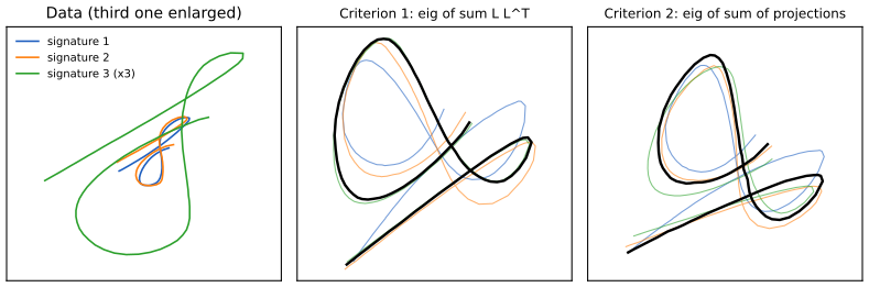
Figure 13.S1 (supplementary, Exercise 13.6). Left: the three signatures of the book's website, the third enlarged three times. Middle: the criterion-1 average (black) and each signature after its best affine map; the enlarged signature dominates. Right: the affine-invariant criterion-2 average. Code: fig_13_s1. Download: PDF · SVGExercise 13.7. For nearest neighbours on the "easy" and "hard" problems of Figure 13.5: (1) replicate the left panels; (2) estimate the errors by five-fold cross-validation and compare; (3) add \(2t/N\) to the training error, with \(t=N/r\) the approximate number of parameters for \(r\) neighbours, and compare. Which estimates the best number of neighbours better, CV or the AIC-like criterion?
Solution
(1) Figure 13.5 (left panels) is the replication. (2)–(3) On each of the ten training sets the code computes the five-fold CV error and the penalised training error \(\text{err}+2/r\) for \(r=1,5,\dots,69\), picks \(r\) by each, and records the test error at the choice (
ex137_summary, Figure 13.S2).Problem best \(r\) (test) \(r\) by CV \(r\) by AIC-like test error at CV choice at AIC choice best possible easy 29 17 37 0.131 0.132 0.124 difficult 1 1 61 0.456 0.494 0.425 (The \(r\) columns minimise the averaged curves; the error columns average the errors at each realisation's own choice.) The CV curve tracks the test curve in shape, sitting slightly above it (it trains on 80 points, not 100). The AIC-like curve is fine on the easy problem, where the training error is a reasonable proxy, but fails on the difficult one: the training error of k-NN counts the point itself among its neighbours, so it is 0 at \(r=1\) and grows quickly, and the penalty \(2/r\) is too crude to compensate; it picks \(r=61\), a near-coin-toss rule. CV is the better guide. (\(N/r\) is the effective number of parameters of k-NN regression, \(\Tr\bm S=N/r\), Section 7.6; for classification with 0–1 loss the optimism has no such simple form.)
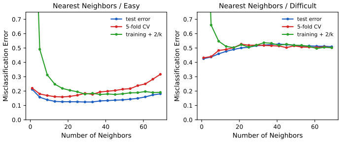
Figure 13.S2 (supplementary, Exercise 13.7). Means over ten realisations of the test error, the five-fold CV error and the AIC-like training error \(+\,2/r\). Code: fig_13_s2. Download: PDF · SVGExercise 13.8. Two classes with two independent \(N(\cdot,1)\) features, means \((-1,-1)\) and \((1,1)\); each feature vector is rotated by its own random angle \(\theta\sim U(0,2\pi)\). Take 50 training and 500 test points per class and compare (1) nearest neighbours, (2) nearest neighbours with hints (ten randomly rotated copies of each training point), (3) nearest neighbours with the rotation-invariant Euclidean metric, (4) tangent distance; choose the number of neighbours by tenfold CV.
Solution
Note on the book: as stated, the two classes are identical
After a uniform random rotation about the origin, the distribution of a point depends only on the distribution of its radius, and the density is \(f_k(x)=f_{R,k}(\|x\|)/(2\pi\|x\|)\). In class \(k\), \(\|X\|\) is the norm of \(N(\mu_k,\bI_2)\), whose distribution (Rice) depends on \(\mu_k\) only through \(\|\mu_k\|\). Both means have norm \(\sqrt2\), so the two classes have the same distribution and the Bayes error is \(\frac12\): no classifier can do better than chance. Simulation confirms it (a two-sample test cannot distinguish the radii of 20,000 points per class), and the four methods have mean test errors 0.498, 0.489, 0.497 and 0.495 over 20 realisations. To make the exercise informative the means must have different norms; below, class 2 has mean \((2,2)\).
The invariant metric. For rotations about the origin, \(\min_{\phi,\psi}\|R_\phi x-R_\psi y\|=\min_\phi\|R_\phi x-y\|=\big|\|x\|-\|y\|\big|\): by the reverse triangle inequality \(\|R_\phi x-y\|\ge\big|\|R_\phi x\|-\|y\|\big|=\big|\|x\|-\|y\|\big|\), with equality when \(R_\phi x\) points in the direction of \(y\). So invariant-metric 1-NN is nearest neighbours on the radius.
Tangent distance. The rotation tangent at \(x\) is \(t_x=(-x_2,x_1)\). In \(\R^2\) two tangent lines are almost never parallel, so the two-sided tangent distance is almost always 0 (the "lines intersect" situation of Figure 13.11 that the book says does not happen in \(\R^{256}\)). Use the one-sided version: the distance from the query \(y\) to the tangent line of the training point \(x\) is the component of \(y-x\) along \(x/\|x\|\), i.e. \(\big|y^\T x/\|x\|-\|x\|\big|\).
Results (class means \((-1,-1)\) and \((2,2)\), Bayes rate 0.254 by integration over the radius; mean test error over 20 realisations, \(k\) by tenfold CV with all copies of a point kept in one fold for the hints): nearest neighbours 0.321, with hints 0.274, invariant metric 0.264, one-sided tangent distance 0.385. The invariant metric is best and almost reaches the Bayes rate, because it reduces the problem to one dimension; hints approximate it with ten copies per point. Tangent distance is worst: the tangent line is a good approximation to the circle of rotations only for small angles, while here the transformations are arbitrary rotations, so it measures something that is neither Euclidean nor invariant. This is the situation the book warns about: tangent distance suits small transformations (
exercise_13_8).
Demonstrations for this chapter
Each demonstration runs in the browser and links back to these notes. The ▶ Demo boxes above open them already set to the case under discussion.
| Demonstration | What you can see | Sections and results |
|---|---|---|
| K-means and LVQ prototypes | K-means prototypes per class and LVQ1 from them, on the three-class simulation and the mixture data: the paths of the prototypes, the boundaries, the test error pass by pass and against \(R\). Presets: 1 K-means (Fig 13.1 top); 2 LVQ (Fig 13.1 bottom); 3 mixture data (Fig 13.2); 4 learning rate too large; 5 one prototype per class. | 13.2.1, 13.2.2; Algorithm 13.1, Result 13.3 |
| The k-NN error and the Cover–Hart bound | A spiral problem with known posteriors: the exact \(E^*\), \(E_1\) and bound, the expected k-NN error against \(k\) and against \(N\), and the asymptotic k-NN curve. Presets: 1 \(N=100\); 2 \(N=10{,}000\); 3 sharp classes; 4 noisy classes; 5 three classes. | 13.3; Results 13.6, 13.7, Exercise 13.3 |
| DANN neighbourhoods | The DANN metric at a movable query point on the ring and strip data: the estimation neighbourhood, the DANN and Euclidean k-NN neighbourhoods, the sphered picture, and the test error against \(\epsilon\). Presets: 1 boundary (Fig 13.14); 2 pure region; 3 \(\epsilon=0\); 4 large \(\epsilon\); 5 vertical boundary (Fig 13.13). | 13.4; Results 13.10, 13.11 |
Related demonstrations: in this course, the least squares and k-NN demo and the curse of dimensionality demo (Chapter 2) and the mixture discriminant analysis demo (Chapter 12); in the companion courses, the K-means and EM demo and the K-means vector quantisation demo. The Python code that produces every figure of this page is code/ch13_prototypes_nearest_neighbors.py (see the code index).
References
- Hastie, T., Tibshirani, R. and Friedman, J. (2009). The Elements of Statistical Learning: Data Mining, Inference, and Prediction, 2nd edition. Springer, New York. Chapter 13, pp. 459–483. hastie.su.domains/ElemStatLearn.
- Abu-Mostafa, Y. (1995). Hints. Neural Computation, 7(4), 639–671.
- Cover, T. and Hart, P. (1967). Nearest neighbor pattern classification. IEEE Transactions on Information Theory, 13(1), 21–27.
- Dasarathy, B. (1991). Nearest Neighbor Pattern Classification Techniques. IEEE Computer Society Press, Los Alamitos, CA.
- Devijver, P. and Kittler, J. (1982). Pattern Recognition: A Statistical Approach. Prentice-Hall, Englewood Cliffs, NJ.
- Duan, N. and Li, K.-C. (1991). Slicing regression: a link-free regression method. The Annals of Statistics, 19(2), 505–530.
- Fix, E. and Hodges, J. (1951). Discriminatory analysis: nonparametric discrimination, consistency properties. Technical report 21-49-004, USAF School of Aviation Medicine, Randolph Field, TX.
- Friedman, J. (1994a). Flexible metric nearest neighbor classification. Technical report, Stanford University.
- Friedman, J., Baskett, F. and Shustek, L. (1975). An algorithm for finding nearest neighbors. IEEE Transactions on Computers, 24(10), 1000–1006.
- Friedman, J., Bentley, J. and Finkel, R. (1977). An algorithm for finding best matches in logarithmic expected time. ACM Transactions on Mathematical Software, 3(3), 209–226.
- Hart, P. (1968). The condensed nearest-neighbor rule. IEEE Transactions on Information Theory, 14(3), 515–516.
- Hastie, T. and Simard, P. (1998). Models and metrics for handwritten digit recognition. Statistical Science, 13(1), 54–65.
- Hastie, T. and Tibshirani, R. (1996a). Discriminant adaptive nearest-neighbor classification. IEEE Transactions on Pattern Analysis and Machine Intelligence, 18(6), 607–616.
- Kohonen, T. (1989). Self-Organization and Associative Memory, 3rd edition. Springer, Berlin.
- Lloyd, S. (1957). Least squares quantization in PCM. Technical report, Bell Laboratories; published in IEEE Transactions on Information Theory, 28(2), 129–137 (1982).
- MacQueen, J. (1967). Some methods for classification and analysis of multivariate observations. In Proceedings of the Fifth Berkeley Symposium on Mathematical Statistics and Probability, Vol. 1, 281–297.
- Michie, D., Spiegelhalter, D. and Taylor, C. (eds) (1994). Machine Learning, Neural and Statistical Classification. Ellis Horwood, New York.
- Myles, J. and Hand, D. (1990). The multi-class metric problem in nearest neighbour discrimination rules. Pattern Recognition, 23(11), 1291–1297.
- Ripley, B. D. (1996). Pattern Recognition and Neural Networks. Cambridge University Press.
- Robbins, H. and Monro, S. (1951). A stochastic approximation method. The Annals of Mathematical Statistics, 22(3), 400–407.
- Short, R. and Fukunaga, K. (1981). The optimal distance measure for nearest neighbor classification. IEEE Transactions on Information Theory, 27(5), 622–627.
- Simard, P., Le Cun, Y. and Denker, J. (1993). Efficient pattern recognition using a new transformation distance. In Advances in Neural Information Processing Systems 5, Morgan Kaufmann, 50–58.
- Stone, C. (1977). Consistent nonparametric regression. The Annals of Statistics, 5(4), 595–645.
The numerical statements in the text (the K-means and LVQ properties and the LVQ fixed point, the agreement of the k-NN code with a library implementation, the Cover–Hart inequalities and the convergence of 1-NN on the spiral problem, the centroid facts of the comparative study, the tangent vectors against finite differences and the closed-form tangent distance, the median radius against simulation, the DANN identities and the chi-squared expansion, the global-reduction identity, the condensing property, the exercises' numbers and the notes on the book) were confirmed numerically.