Single-layer Networks: Classification
A classifier assigns an input \(\mathbf{x}\in\R^D\) to one of \(K\) classes. This chapter studies the models whose decision surfaces are hyperplanes: one layer of weights followed, at most, by a fixed output nonlinearity. It meets them three times. First as discriminant functions fitted directly (least squares). Then through decision theory, which says what an optimal decision is once the posterior probabilities are known, and how to measure a classifier (confusion matrix, precision, recall, ROC curve). Then as probabilistic models: generative (class densities plus Bayes' theorem, which produces a logistic sigmoid or softmax of linear functions) and discriminative (logistic, softmax and probit regression fitted by maximum likelihood). The chapter ends with the pairing of output activation and error function, the canonical link, that the rest of the book uses for deep networks. Every step the book leaves to the reader is written out below.
Ch. 1 Deep learning revolution Ch. 2 Probabilities Ch. 3 Standard distributions Ch. 4 Regression Ch. 5 Classification Ch. 6 Deep neural networks Ch. 7 Gradient descent Ch. 8 Backpropagation Ch. 9 Regularization Ch. 10 Convolutional networks Ch. 11 Structured distributions Ch. 12 Transformers Ch. 13 Graph neural networks Ch. 14 Sampling Ch. 15 Discrete latent variables Ch. 16 Continuous latent variables Ch. 17 GANs Ch. 18 Normalizing flows Ch. 19 Autoencoders Ch. 20 Diffusion models Appendices A to C
How to read these notes
They follow the book. Sections carry the book's numbers (5.1, 5.4.3, ...) and every displayed equation that appears in the book carries the book's own equation number, e.g. (5.75), so the notes can be read next to the book. Equations without a number are steps that the book skips.
Filling the gaps. Wherever the book says that a result is easily verified, states a property without proof, or leaves it as an exercise, an orange Filling the gap box or a proof gives the complete argument. Proofs start hidden: open one with its bar, or use the button below.
Figures, code and demonstrations. Every figure of the chapter that is computed from a model or from data is reproduced from scratch by the Python code. The ▶ Demo boxes open an interactive demonstration already set to the case being discussed.
Main reference
C. M. Bishop and H. Bishop, Deep Learning: Foundations and Concepts, Springer (2024), Chapter 5, pages 131–169. Section, equation, figure and exercise numbers below refer to this book; its website is www.bishopbook.com. The exercises are compared with the official solutions manual (version 1.0).
The explanations, derivations, figures and code are my own; equations are cited by their numbers in the book.
Companion course
Most of this chapter overlaps the companion course Bayesian and Probabilistic Machine Learning (Bishop 2006), where several of these results are proved in full. Where the statement is the same, the notes below give it with a short proof and link the full derivation there.
- Discriminant functions, least squares for classification: Section 4.1 (4.1.1–4.1.3) ↔ Section 5.1 here.
- Decision theory (misclassification rate, expected loss, reject option, inference and decision): Section 1.5 ↔ Sections 5.2.1–5.2.4 here. Classifier accuracy and ROC curves (5.2.5, 5.2.6) are new in this book and are treated in full here.
- Generative classifiers: Section 4.2 ↔ Section 5.3 here; the exponential family: Section 2.4.
- Discriminative classifiers (logistic regression, IRLS, softmax, probit, canonical links): Section 4.3 ↔ Section 5.4 here.
- Demonstrations there: decision theory, least squares, Fisher and the perceptron, logistic regression with IRLS, probit and the Laplace approximation.
The chapter at a glance
- 5.1 A linear discriminant \(y(\mathbf{x})=\mathbf{w}^\T\mathbf{x}\)
\({}+w_0\) cuts space with a hyperplane; \(y(\mathbf{x})/\|\mathbf{w}\|\) is the signed distance to it. \(K\) classes need \(K\) linear functions compared by "largest wins" (the regions are then convex); gluing two-class classifiers together leaves ambiguous regions. Least squares on 1-of-\(K\) targets has a closed form and its outputs sum to one, but it is not robust: far, correctly classified points pull the boundary. - 5.2 With the posteriors \(p(\cC{k}\given\mathbf{x})\) known, the fewest mistakes come from choosing the largest posterior, the smallest expected loss from minimising \(\sum_kL_{kj}p(\cC{k}\given\mathbf{x})\), and rejecting where the largest posterior is below \(\theta\) lowers the error on the rest. Accuracy, precision, recall, the F-score and the ROC curve describe performance; the ROC curve of the posterior threshold dominates every other classifier (Neyman–Pearson) and its area is the probability that a positive scores above a negative.
- 5.3 Bayes' theorem writes the posterior as \(\sigma(a)\) or a softmax of \(a_k\)
\({}=\ln p(\mathbf{x}\given\cC{k})p(\cC{k})\). Gaussian classes with a shared covariance, naive Bayes discrete features and exponential-family classes with a shared scale all make \(a_k\) linear in \(\mathbf{x}\); maximum likelihood gives class fractions, class means and the pooled covariance. - 5.4 Fit the posterior directly: logistic regression has \(M\) parameters instead of \(M(M+5)/2+1\), a convex cross-entropy with gradient \(\sum_n(y_n-t_n)\bm\phi_n\), and no maximum on separable data. Softmax regression has the same gradient form, probit regression is less robust to mislabelled points, and the "error times input" gradient is a general consequence of the canonical link.
Notation. Inputs \(\mathbf{x}\in\R^D\), features \(\bm\phi=\bm\phi(\mathbf{x})\in\R^M\) (with \(\phi_0=1\) when a bias is wanted), training pairs \((\mathbf{x}_n,\mathbf{t}_n)\), \(n=1,\dots,N\), with \(N_k\) points in class \(\cC{k}\). Two-class targets are \(t\in\{0,1\}\); \(K\)-class targets use the 1-of-\(K\) code. \(\sigma(a)=1/(1+e^{-a})\) is the logistic sigmoid and \(\Phi(a)\) the standard normal distribution function. \(L_{kj}\) is the loss for deciding \(\cC{j}\) when the truth is \(\cC{k}\). \(\Ind[\cdot]\) is the indicator function.
Prerequisites. Linear regression and the pseudo-inverse (Chapter 4 of the book), Gaussian maximum likelihood and the exponential family (Chapter 3; companion course Chapter 2), the chain rule and gradients of quadratic forms.
pp. 131–132 The book distinguishes three ways to build a classifier, in increasing order of what they model: a discriminant function maps \(\mathbf{x}\) straight to a class; a discriminative probabilistic model represents \(p(\cC{k}\given\mathbf{x})\) directly; a generative probabilistic model represents \(p(\mathbf{x}\given\cC{k})\) and \(p(\cC{k})\) and obtains the posterior from Bayes' theorem,
\[ p(\cC{k}\given\mathbf{x})=\frac{p(\mathbf{x}\given\cC{k})\,p(\cC{k})}{p(\mathbf{x})}. \tag{5.1} \]5.1 Discriminant functions
See also: companion course, Section 4.1, discriminant functions (which also covers Fisher's discriminant and the perceptron, not in this book).
Definition 5.1 (decision regions, linear separability) pp. 131–132
A classifier splits the input space into decision regions \(\cR{k}\) (the inputs assigned to \(\cC{k}\)); their boundaries are decision boundaries or decision surfaces. The classifier is linear if the boundaries are pieces of hyperplanes, i.e. \((D-1)\)-dimensional affine subspaces. A two-class data set is linearly separable if there are \(\mathbf{w},w_0\) with \(\mathbf{w}^\T\mathbf{x}_n+w_0>0\) for every point of one class and \(<0\) for every point of the other.
5.1.1 Two classes
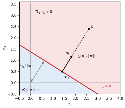
pp. 132–133 The simplest discriminant is an affine function of the input,
\[ y(\mathbf{x})=\mathbf{w}^\T\mathbf{x}+w_0, \tag{5.2} \]with the rule "assign \(\mathbf{x}\) to \(\cC{1}\) if \(y(\mathbf{x})\ge0\), otherwise to \(\cC{2}\)". The weight vector \(\mathbf{w}\) sets the orientation of the surface \(y(\mathbf{x})=0\) and the bias \(w_0\) its position.
Result 5.1 (geometry of a linear discriminant) pp. 132–133, (5.3)–(5.6), Figure 5.1
Assume \(\mathbf{w}\ne\mathbf{0}\). (a) \(\mathbf{w}\) is orthogonal to every vector lying in the surface \(y=0\). (b) For \(\mathbf{x}\) on the surface,
\[ \frac{\mathbf{w}^\T\mathbf{x}}{\|\mathbf{w}\|}=-\frac{w_0}{\|\mathbf{w}\|}, \tag{5.3} \]so \(-w_0/\|\mathbf{w}\|\) is the signed distance from the origin to the surface. (c) Every \(\mathbf{x}\) decomposes as
\[ \mathbf{x}=\mathbf{x}_\perp+r\,\frac{\mathbf{w}}{\|\mathbf{w}\|},\qquad r=\frac{y(\mathbf{x})}{\|\mathbf{w}\|}, \tag{5.4, 5.5} \]where \(\mathbf{x}_\perp\) is the point of the surface closest to \(\mathbf{x}\); \(|r|\) is the distance from \(\mathbf{x}\) to the surface and the sign of \(r\) says on which side \(\mathbf{x}\) lies. (d) With \(\tilde{\mathbf{w}}=(w_0,\mathbf{w})\) and \(\tilde{\mathbf{x}}=(1,\mathbf{x})\), \(y(\mathbf{x})\)
Proof
(a) If \(y(\mathbf{x}_A)=y(\mathbf{x}_B)=0\), subtracting gives \(\mathbf{w}^\T(\mathbf{x}_A\)
5.1.2 Multiple classes
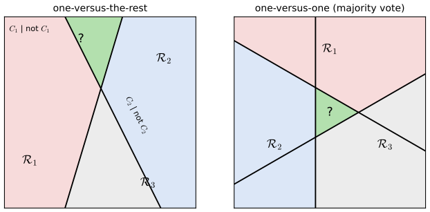
pp. 134–135 Building a \(K\)-class classifier from two-class ones runs into trouble. A one-versus-the-rest scheme uses \(K-1\) classifiers "\(\cC{k}\) or not"; a one-versus-one scheme uses \(K(K-1)/2\) classifiers, one per pair, and a majority vote. Both leave regions where the class is not determined (Figure 5.2). A single \(K\)-class discriminant avoids this:
\[ y_k(\mathbf{x})=\mathbf{w}_k^\T\mathbf{x}+w_{k0},\qquad \text{assign }\mathbf{x}\text{ to }\cC{k}\text{ if }y_k(\mathbf{x})>y_j(\mathbf{x})\text{ for all }j\ne k, \tag{5.7} \]and the boundary between \(\cC{k}\) and \(\cC{j}\) is the hyperplane
\[ (\mathbf{w}_k-\mathbf{w}_j)^\T\mathbf{x}+(w_{k0}-w_{j0})=0. \tag{5.8} \]Filling the gap 5.1: why glued two-class classifiers leave ambiguous regions p. 134, Figure 5.2
The book shows pictures; here is the argument behind them, for \(D=2\) and \(K=3\).
Derivation
One versus the rest. Take the \(K-1=2\) classifiers \(y_1\) ("\(\cC{1}\) if \(y_1>0\)") and \(y_2\) ("\(\cC{2}\) if \(y_2>0\)"); a point that both reject is put in \(\cC{3}\). If the two lines are not parallel they cross, and the four sign patterns \((\pm,\pm)\) all occur, each on an unbounded wedge. On the wedge where \(y_1>0\) and \(y_2>0\) both classifiers claim the point: it is ambiguous. (With \(K\) classifiers, one per class, there is in addition a region claimed by nobody when the lines are in general position.) The ambiguity disappears only for special configurations, e.g. parallel lines oriented so that the "both" wedge is empty.
One versus one. For each pair \(i<j\) let \(s_{ij}(\mathbf{x})\) be affine, voting \(\cC{i}\) if \(s_{ij}>0\) and \(\cC{j}\) otherwise. At each \(\mathbf{x}\) the three votes form a tournament on three classes: either one class wins both its contests (a unique winner with two votes), or the votes are cyclic (\(\cC{1}\) beats \(\cC{2}\), \(\cC{2}\) beats \(\cC{3}\), \(\cC{3}\) beats \(\cC{1}\)) and every class has exactly one vote, a three-way tie. Three lines in general position bound a triangle, and the sign pattern inside it is the one obtained by flipping, relative to any outside cell, the signs of the lines one crosses to get in. Choosing the orientations so that the pattern inside is cyclic (our Figure 5.2 does this explicitly, with offsets \(+0.45,+0.45,-0.45\) of the three bisectors) produces a bounded ambiguous triangle. So majority voting is not well defined everywhere. ∎
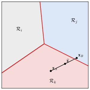
Result 5.2 (the regions of a linear \(K\)-class discriminant are convex) p. 135, (5.9), (5.10), Figure 5.3
Each decision region of (5.7) is an intersection of \(K-1\) open half-spaces, hence convex; in particular it is connected, and it has no holes.
Proof
By (5.7), \(\mathbf{x}\in\cR{k}\) if and only if \((\mathbf{w}_k\)
A numerical test draws 1200 random segments with both ends in the same region of a random four-class discriminant and finds no segment that leaves its region.
5.1.3 1-of-K coding
pp. 135–136 Two classes are coded by \(t\in\{0,1\}\) (\(t=1\) for \(\cC{1}\)). For \(K>2\) classes the 1-of-\(K\) or one-hot code uses a vector with a single 1 in the position of the class; for \(K=5\) and class 2,
\[ \mathbf{t}=(0,1,0,0,0)^\T. \tag{5.11} \]Result 5.3 (the regression function of a 1-of-K target is the posterior; Exercise 5.1) p. 136
\(\E[\mathbf{t}\given\mathbf{x}]\)
Proof
Component \(t_k\) is 1 exactly when the class is \(\cC{k}\), so \(\E[t_k\given\mathbf{x}]\)
5.1.4 Least squares for classification
See also: companion course, Section 4.1.3, least squares for classification (Filling the gap 4.1, Result 4.3).
pp. 136–137 Fit each class score by its own linear model,
\[ y_k(\mathbf{x})=\mathbf{w}_k^\T\mathbf{x}+w_{k0},\qquad \mathbf{y}(\mathbf{x})=\widetilde{\mathbf{W}}^\T\tilde{\mathbf{x}}, \tag{5.12, 5.13} \]where column \(k\) of \(\widetilde{\mathbf{W}}\) is \(\tilde{\mathbf{w}}_k\)
Filling the gap 5.2: from (5.14) to (5.15) p. 136
The book says "setting the derivative with respect to \(\widetilde{\mathbf{W}}\) to zero". Here is that derivative, and when the solution is unique.
Derivation
Write the trace as a double sum: \(E_D\)
\(E_D\) is a convex quadratic (its Hessian in each column is \(\widetilde{\mathbf{X}}^\T\widetilde{\mathbf{X}}\), positive semi-definite), so every stationary point is a global minimum, and the stationary points solve the normal equations \(\widetilde{\mathbf{X}}^\T\widetilde{\mathbf{X}}\widetilde{\mathbf{W}}\)
Result 5.4 (linear constraints on the targets are inherited; Exercises 5.3, 5.4) p. 137, (5.17), (5.18)
Suppose \(\widetilde{\mathbf{X}}\) has full column rank and its first column is all ones (a bias input). If every target satisfies \(\mathbf{A}\mathbf{t}_n+\mathbf{b}\)
and likewise \(\mathbf{A}\mathbf{y}(\mathbf{x})\)
Proof
The constraints say \(\mathbf{T}\mathbf{A}^\T=\)
since the first entry of \(\tilde{\mathbf{x}}\) is 1. One constraint is the case of a single row. This route avoids the centring argument of the solutions manual and makes clear where the bias is needed: without a constant input, \(\one_N\) need not lie in the column space of \(\widetilde{\mathbf{X}}\) and the conclusion fails. ∎
Filling the gap 5.3: what least squares estimates, and why it is not robust pp. 136–137, Figure 5.4
The book says least squares "approximates the conditional expectation" and "gives too much weight to data points that are a long way from the decision boundary". Both statements can be made precise.
Derivation
What it estimates. By Result 5.3 the unrestricted minimiser of \(\E\|\mathbf{y}(\mathbf{x})\)
Why far points pull. Take two classes with targets \(t\in\{0,1\}\), a single output \(y\)
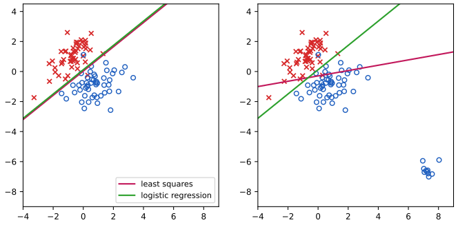
fig_5_4. Download: PDF · SVGThe failure is not surprising: least squares is maximum likelihood for Gaussian noise, and a 0/1 target is as far from Gaussian as a distribution can be. The probabilistic models of Sections 5.3 and 5.4 replace it.
5.2 Decision theory
See also: companion course, Section 1.5, decision theory (Results 1.15–1.17, Filling the gap 1.4) and its decision theory demo.
pp. 138–139 Prediction splits into inference (learning \(p(\mathbf{x},\mathcal{C}_k)\) or \(p(\cC{k}\given\mathbf{x})\) from data, the hard part) and decision (choosing an action given those probabilities, usually easy). The running example is a skin-lesion image \(\mathbf{x}\), with \(\cC{1}\) = no cancer ("normal") and \(\cC{2}\) = cancer. Bayes' theorem,
\[ p(\cC{k}\given\mathbf{x})=\frac{p(\mathbf{x}\given\cC{k})p(\cC{k})}{p(\mathbf{x})}, \tag{5.19} \]turns the prior \(p(\cC{k})\) (how common cancer is before the image is seen) into the posterior. (The book writes "\(p(\cC{1})\) represents the probability that a person has cancer"; with its own labelling that is \(p(\cC{2})\). See the corrections.)
5.2.1 Misclassification rate
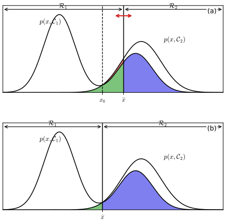
pp. 139–140 A decision rule is a partition of input space into regions \(\cR{1},\dots,\cR{K}\). For two classes
\[ p(\text{mistake})=p(\mathbf{x}\in\cR{1},\cC{2})+p(\mathbf{x}\in\cR{2},\cC{1})=\int_{\cR{1}}p(\mathbf{x},\cC{2})\,\d\mathbf{x}+\int_{\cR{2}}p(\mathbf{x},\cC{1})\,\d\mathbf{x}, \tag{5.20} \] \[ p(\text{correct})=\sum_{k=1}^K\int_{\cR{k}}p(\mathbf{x},\cC{k})\,\d\mathbf{x}. \tag{5.21} \]Result 5.5 (the largest posterior gives the fewest mistakes) p. 140
Among all decision rules, including randomised ones, \(p(\text{correct})\) is maximised by assigning each \(\mathbf{x}\) to a class with the largest posterior \(p(\cC{k}\given\mathbf{x})\), and the minimum probability of a mistake is \(1\)
Proof
A (possibly randomised) rule assigns \(\mathbf{x}\) to \(\cC{k}\) with probability \(\delta_k(\mathbf{x})\ge0\), \(\sum_k\delta_k=1\); a deterministic rule has \(\delta_k=\Ind[\mathbf{x}\in\cR{k}]\). Then \(p(\text{correct})\)
5.2.2 Expected loss
pp. 140–142 When mistakes have different costs, a loss matrix \(L_{kj}\) (true class \(k\), decision \(j\)) records them; for the screening problem the book uses the matrix of Figure 5.6. The average loss of a rule with regions \(\cR{j}\) is
\[ \E[L]=\sum_k\sum_j\int_{\cR{j}}L_{kj}\,p(\mathbf{x},\cC{k})\,\d\mathbf{x}. \tag{5.22} \]| true \ decided | normal | cancer |
|---|---|---|
| normal | 0 | 1 |
| cancer | 100 | 0 |
Result 5.6 (minimum expected loss; Exercises 5.7, 5.8) p. 142, (5.23)
The expected loss (5.22) is minimised by assigning each \(\mathbf{x}\) to a class \(j\) that minimises
\[ \sum_kL_{kj}\,p(\cC{k}\given\mathbf{x}). \tag{5.23} \]For two classes with \(L_{11}=L_{22}=0\) this means: decide \(\cC{2}\) when
\[ p(\cC{2}\given\mathbf{x})\ \ge\ \tau^\star=\frac{L_{12}}{L_{12}+L_{21}}, \]so with the matrix of Figure 5.6, "cancer" as soon as \(p(\cC{2}\given\mathbf{x})\ge1/101\)
Proof
Exactly as in Result 5.5: for a randomised rule \(\delta_j(\mathbf{x})\), \(\E[L]\)
The rule needs only the posteriors; if the loss matrix changes, the decisions change with no retraining. A direct computation confirms on the demo's one-dimensional problem that \(\tau^\star\) beats 99 other thresholds.
5.2.3 The reject option
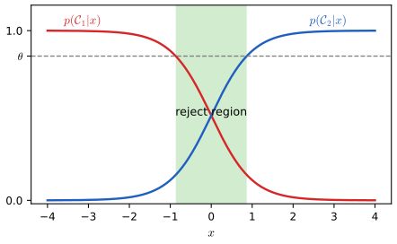
pp. 142–143 Where the largest posterior is well below one, decisions are unreliable. The reject option refuses to decide (e.g. sends the case to a human) when \(\max_kp(\cC{k}\given\mathbf{x})\)
Result 5.7 (the reject option; Exercise 5.10) p. 143, Figure 5.7
(a) \(\theta=1\) rejects every input; any \(\theta<1/K\) rejects none. (b) If rejecting costs \(\lambda\) and deciding \(j\) costs \(L_{kj}\) when the truth is \(k\), the minimum-expected-loss rule is: compute \(r_j(\mathbf{x})\)
Proof
(a) The posteriors are \(K\) numbers summing to one, so the largest is at least \(1/K>\theta\); and it is at most \(1=\theta\). (b) Rejection is one more action with conditional risk \(\lambda\) (the same whatever the class); by the pointwise argument of Result 5.6 the best action at \(\mathbf{x}\) is the one with the smallest conditional risk among \(r_1(\mathbf{x}),\dots,r_K(\mathbf{x}),\lambda\). (c) Then \(\min_jr_j=1\)
Filling the gap 5.4: rejecting lowers the error on the inputs that are kept p. 142
The book motivates rejection by "a lower error rate on those examples for which a classification decision is made". This is true for every threshold, not just on average.
Derivation
Let \(M=\max_kp(\cC{k}\given\mathbf{x})\) for \(\mathbf{x}\sim p(\mathbf{x})\). With the largest-posterior decision, the probability of a mistake at \(\mathbf{x}\) is \(1-M\), so the error rate on the accepted inputs is \(e(\theta)=\E[1-M\given M>\theta]\). Take \(\theta<\theta'\) with \(P(M>\theta')>0\). The event \(\{M>\theta\}\) is the disjoint union of \(\{M>\theta'\}\) and \(\{\theta<M\le\theta'\}\), so \(e(\theta)\) is a weighted average of \(\E[1-M\given M>\theta']\le1-\theta'\) and \(\E[1-M\given\theta<M\le\theta']\ge1\)
5.2.4 Inference and decision
pp. 143–147 There are three ways to solve a classification problem: (a) generative: model \(p(\mathbf{x}\given\cC{k})\) and \(p(\cC{k})\), then use
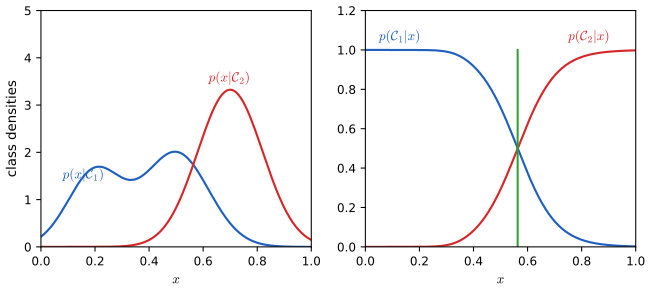
\[ p(\cC{k}\given\mathbf{x})=\frac{p(\mathbf{x}\given\cC{k})p(\cC{k})}{p(\mathbf{x})},\qquad p(\mathbf{x})=\sum_kp(\mathbf{x}\given\cC{k})p(\cC{k}); \tag{5.24, 5.25} \](b) discriminative: model \(p(\cC{k}\given\mathbf{x})\) directly; (c) a discriminant function \(f(\mathbf{x})\) that outputs a class, with no probabilities. (a) is the most demanding but also gives \(p(\mathbf{x})\), useful for novelty detection. Much of the structure of \(p(\mathbf{x}\given\cC{k})\) may be irrelevant to the posterior (Figure 5.8). Posteriors, however, are worth having: for minimising risk when the loss matrix changes, for the reject option, for correcting for class priors, and for combining models.
Filling the gap 5.5: correcting for class priors, and combining models pp. 145–147, (5.26), (5.27)
The book describes both procedures in words; here are the formulas, the assumptions they need, and the proofs.
Derivation
Prior correction. Suppose the model was trained on a re-balanced data set with class fractions \(\pi'_k\) (e.g. equal), whereas the population has priors \(\pi_k\). The assumption that makes correction possible is that re-balancing samples whole classes, so the class-conditional densities \(p(\mathbf{x}\given\cC{k})\) are the same in both. Then the trained model approximates \(p'(\cC{k}\given\mathbf{x})\)
because the common factor \(Z'(\mathbf{x})\) cancels: divide by the training fractions, multiply by the population priors, normalise. A discriminant function has no posterior to correct, which is the book's point.
Combining models. Assume conditional independence given the class, \(p(\mathbf{x}_I,\mathbf{x}_B\given\cC{k})\)
the proportionality being in \(k\), so normalising over \(k\) gives the posterior. The joint marginal \(p(\mathbf{x}_I,\mathbf{x}_B)\)
5.2.5 Classifier accuracy
pp. 147–148 Call "cancer" the positive class. Each tested person is a true positive, false positive (type 1 error), true negative or false negative (type 2 error), with counts adding to
\[ N=N_\mathrm{TP}+N_\mathrm{FP}+N_\mathrm{TN}+N_\mathrm{FN}, \tag{5.28} \]arranged in the confusion matrix of Figure 5.9. The usual summaries are
\[ \text{Accuracy}=\frac{N_\mathrm{TP}+N_\mathrm{TN}}{N},\quad \text{Precision}=\frac{N_\mathrm{TP}}{N_\mathrm{TP}+N_\mathrm{FP}},\quad \text{Recall}=\frac{N_\mathrm{TP}}{N_\mathrm{TP}+N_\mathrm{FN}}, \tag{5.29–5.31} \] \[ \text{False positive rate}=\frac{N_\mathrm{FP}}{N_\mathrm{FP}+N_\mathrm{TN}},\qquad \text{False discovery rate}=\frac{N_\mathrm{FP}}{N_\mathrm{FP}+N_\mathrm{TP}}. \tag{5.32, 5.33} \]Precision estimates \(P(\text{cancer}\given\text{test positive})\), recall (the true positive rate, sensitivity) \(P(\text{test positive}\given\text{cancer})\), the false positive rate \(P(\text{test positive}\given\text{normal})\). Accuracy is misleading with rare classes: if 1 in 1000 has cancer, "nobody has cancer" is 99.9% accurate and useless.
| true \ decided | normal | cancer |
|---|---|---|
| normal | \(N_\mathrm{TN}\) | \(N_\mathrm{FP}\) |
| cancer | \(N_\mathrm{FN}\) | \(N_\mathrm{TP}\) |
Result 5.8 (the F-score; Exercise 5.5) p. 150, (5.38), (5.39)
The F-score is the harmonic mean of precision \(P\) and recall \(R\) (the book's text says "geometric mean", a slip):
\[ F=\frac{2PR}{P+R}=\frac{2N_\mathrm{TP}}{2N_\mathrm{TP}+N_\mathrm{FP}+N_\mathrm{FN}},\qquad \frac1F=\frac12\Big(\frac1P+\frac1R\Big). \tag{5.38, 5.39} \]It satisfies \(\min(P,R)\le F\le\sqrt{PR}\le(P+R)/2\), so it is dominated by the worse of the two.
Proof
With \(a=N_\mathrm{TP}\), \(P=a/(a+N_\mathrm{FP})\), \(R=a/(a+N_\mathrm{FN})\): \(1/P+1/R=(2a+N_\mathrm{FP}\)
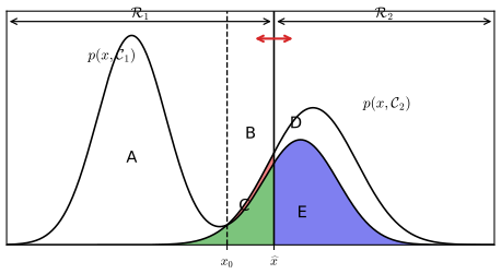
Filling the gap 5.6: the labelled regions of Figure 5.10 p. 148, (5.34)–(5.37)
The book lists \(N_\mathrm{FP}/N=E\), \(N_\mathrm{TP}/N=D+E\), \(N_\mathrm{FN}/N=B+C\), \(N_\mathrm{TN}/N=A+C\) without comment. They hold, but the regions overlap in a way worth seeing.
Derivation
One-dimensional input, \(\cC{2}\) = cancer, rule "cancer if \(x\ge\widehat{x}\)", so \(\cR{1}=\{x<\widehat{x}\}\). Write \(j_k(x)=p(x,\cC{k})\) and \(m=\min(j_1,j_2)\). The letters denote areas: on \(\cR{1}\), \(C=\int_{\cR{1}}m\) (green), \(A=\int_{\cR{1}}(j_1-m)\) (under \(j_1\), above green) and \(B=\int_{\cR{1}}(j_2-m)\) (red); on \(\cR{2}\), where the figure has \(j_2\ge j_1\), \(E=\int_{\cR{2}}j_1\) (blue) and \(D=\int_{\cR{2}}(j_2-j_1)\). As \(N\to\infty\) the law of large numbers turns each count fraction into a probability:
\[ \frac{N_\mathrm{FP}}N\to\int_{\cR{2}}j_1=E,\quad \frac{N_\mathrm{TP}}N\to\int_{\cR{2}}j_2=D+E,\quad \frac{N_\mathrm{FN}}N\to\int_{\cR{1}}j_2=B+C,\quad \frac{N_\mathrm{TN}}N\to\int_{\cR{1}}j_1=A+C. \]The green area \(C\) and the blue area \(E\) lie under both curves, so they are counted twice: the four fractions sum to 1, hence \(A+B+2C+D+2E=1\), not \(A+B+C+D+E=1\). For our Figure 5.10, \((A,B,C,D,E)\)
5.2.6 ROC curve
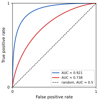
pp. 148–150 A probabilistic classifier says "positive" when its output exceeds a threshold. Sweeping the threshold from \(+\infty\) to \(-\infty\) traces the receiver operating characteristic (ROC) curve: true positive rate against false positive rate. The point \((0,0)\) is "everyone normal", \((1,1)\) "everyone positive", \((0,1)\) perfection; one confusion matrix is one point. The area under the curve (AUC) summarises it.
Result 5.9 (properties of ROC curves) pp. 148–150
Let a classifier have score \(s(\mathbf{x})\), and write \(S_+\), \(S_-\) for the score of a random positive and of a random negative (independent).
- Random guessing, "positive with probability \(\rho\)" regardless of \(\mathbf{x}\), has TPR = FPR = \(\rho\): sweeping \(\rho\) gives the diagonal.
- AUC as a probability. \(\text{AUC}=P(S_+>S_-)+\tfrac12P(S_+\)
\({}=S_-)\). So AUC = 1/2 for a score unrelated to the class and 1 for a perfectly separating one. - Prior invariance. TPR and FPR are conditional on the class, so the ROC curve depends only on \(p(\mathbf{x}\given\cC{k})\), not on the prevalence.
- Optimality (Neyman–Pearson). Among all rules, randomised or not, with false positive rate at most \(\alpha\), the largest true positive rate is achieved by thresholding the likelihood ratio \(\ell(\mathbf{x})\)
\({}=p(\mathbf{x}\given\cC{2})/p(\mathbf{x}\given\cC{1})\), equivalently the posterior \(p(\cC{2}\given\mathbf{x})\). Its ROC curve lies on or above the ROC curve of every other classifier, and it is concave. - Operating point. The expected loss \(\E[L]=L_{12}p(\cC{1})\,\mathrm{FPR}\)
\({}+L_{21}p(\cC{2})\,(1-\mathrm{TPR})\) is minimised on the optimal curve where its slope equals \(L_{12}p(\cC{1})/(L_{21}p(\cC{2}))\), which is the threshold \(\tau^\star\) of Result 5.6.
Proof
(1) The decision is independent of the class, so \(P(\text{positive}\given\cC{2})\)
(2) For continuous scores, at threshold \(c\): \(\mathrm{FPR}(c)=P(S_->c)\), \(\mathrm{TPR}(c)=P(S_+>c)\). As \(c\) decreases, FPR increases, and \(\d\,\mathrm{FPR}=f_-(c)\,(-\d c)\) with \(f_-\) the density of \(S_-\). Hence \(\text{AUC}\)
(3) Immediate from the definitions. In terms of the posterior, changing the prior only relabels the thresholds (\(p(\cC{2}\given\mathbf{x})\ge\tau\) is \(\ell(\mathbf{x})\ge k\) with \(k=\tau p(\cC{1})/((1-\tau)p(\cC{2}))\)), so the set of rules, and the curve, is the same.
(4) Let \(\delta^\star(\mathbf{x})\)
(5) Minimising a linear function of \((\mathrm{FPR},\mathrm{TPR})\) over a concave curve picks the point where the curve is tangent to the level lines \(\mathrm{TPR}\)
Filling the gap 5.7: the ROC curve of a Gaussian score Figure 5.11
The book draws two ROC curves without saying where they come from. Ours are exact curves of a simple model.
Derivation
Let the score be \(\N(0,1)\) for negatives and \(\N(d,1)\) for positives (for two Gaussian classes with a shared covariance, the activation \(a(\mathbf{x})\) of Section 5.3.1 is exactly of this form, with \(d\) the Mahalanobis distance between the means). At threshold \(c\), \(\mathrm{FPR}=1-\Phi(c)\) and \(\mathrm{TPR}=1-\Phi(c-d)=\Phi(d-c)\). Eliminating \(c=\Phi^{-1}(1-\mathrm{FPR})=\)
since \(S_+-S_-\sim\N(d,2)\). For \(d=2\), AUC = 0.921; for \(d=0.9\), 0.738. ∎
A loss matrix and a confusion matrix combine into the empirical loss by multiplying entrywise and summing. ROC curves extend to more classes but quickly become unwieldy.
5.3 Generative classifiers
See also: companion course, Section 4.2, probabilistic generative models (Results 4.8–4.11).
pp. 150–152 For two classes Bayes' theorem can be rewritten exactly as
\[ p(\cC{1}\given\mathbf{x})=\frac{p(\mathbf{x}\given\cC{1})p(\cC{1})}{p(\mathbf{x}\given\cC{1})p(\cC{1})+p(\mathbf{x}\given\cC{2})p(\cC{2})}=\frac1{1+\exp(-a)}=\sigma(a),\qquad a=\ln\frac{p(\mathbf{x}\given\cC{1})p(\cC{1})}{p(\mathbf{x}\given\cC{2})p(\cC{2})}, \tag{5.40, 5.41} \]with the logistic sigmoid
\[ \sigma(a)=\frac1{1+\exp(-a)}, \tag{5.42} \]and for \(K\) classes as the softmax (normalised exponential)
\[ p(\cC{k}\given\mathbf{x})=\frac{p(\mathbf{x}\given\cC{k})p(\cC{k})}{\sum_jp(\mathbf{x}\given\cC{j})p(\cC{j})}=\frac{\exp(a_k)}{\sum_j\exp(a_j)},\qquad a_k=\ln\big(p(\mathbf{x}\given\cC{k})p(\cC{k})\big). \tag{5.45, 5.46} \]These rewrites are content-free until \(a\) has a constrained form; the rest of the section finds class densities that make it linear.
Result 5.10 (properties of the sigmoid and the softmax; Exercises 5.11, 5.18) pp. 151–152, (5.43), (5.44), (5.72)
- \(\sigma(-a)=1-\sigma(a)\) (5.43), \(\sigma'(a)=\sigma(a)(1-\sigma(a))\) (5.72), and the inverse is the logit \(a=\ln\{\sigma/(1-\sigma)\}\) (5.44), the log odds \(\ln\{p(\cC{1}\given\mathbf{x})/p(\cC{2}\given\mathbf{x})\}\).
- The softmax is unchanged if the same constant is added to every \(a_k\); with \(K=2\) it is \(\sigma(a_1-a_2)\).
- If \(a_k>a_j+\Delta\) for all \(j\ne k\), then \(p(\cC{k}\given\mathbf{x})>1-(K\)
\({}-1)e^{-\Delta}\): the softmax is a smoothed "max", and \(\mathrm{softmax}(\mathbf{a}/T)\) tends to the indicator of the largest \(a_k\) as the temperature \(T\to0\).
Proof
(1) \(1-\sigma(a)=\frac{e^{-a}}{1+e^{-a}}\)
5.3.1 Continuous inputs
See also: companion course, Section 4.2.1, continuous inputs (Result 4.9).
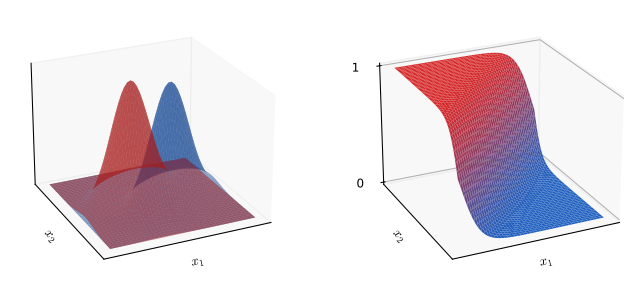
pp. 152–153 Let every class be Gaussian with its own mean and a shared covariance,
\[ p(\mathbf{x}\given\cC{k})=\frac1{(2\pi)^{D/2}}\frac1{|\bm\Sigma|^{1/2}}\exp\Big\{-\frac12(\mathbf{x}-\bm\mu_k)^\T\bm\Sigma^{-1}(\mathbf{x}-\bm\mu_k)\Big\}. \tag{5.47} \]Result 5.11 (a shared covariance gives linear activations; Exercise 5.12) pp. 152–153, (5.48)–(5.53)
Two classes: \(p(\cC{1}\given\mathbf{x})\)
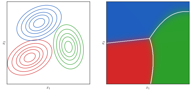
\(K\) classes: the softmax (5.45) of \(a_k(\mathbf{x})\)
(Strictly, (5.46) gives \(a_k\) plus a term common to all classes, which the softmax ignores; (5.51) is \(a_k\) with that term dropped.) The priors enter only the biases, so changing them moves every contour of constant posterior parallel to itself.
Proof
Substitute (5.47) into (5.41). The normalising constants are the same for both classes and cancel, leaving
\[ a=-\tfrac12(\mathbf{x}-\bm\mu_1)^\T\bm\Sigma^{-1}(\mathbf{x}-\bm\mu_1)+\tfrac12(\mathbf{x}-\bm\mu_2)^\T\bm\Sigma^{-1}(\mathbf{x}-\bm\mu_2)+\ln\frac{p(\cC{1})}{p(\cC{2})}. \]Expand each quadratic with the symmetry of \(\bm\Sigma^{-1}\): \((\mathbf{x}\)
Filling the gap 5.8: different covariances give quadratic boundaries p. 153, Figure 5.14
The book says only that the cancellation "will no longer occur". Here is the resulting discriminant.
Derivation
With \(p(\mathbf{x}\given\cC{k})\)
The boundary between \(\cC{k}\) and \(\cC{j}\), \(a_k=a_j\), is \(\tfrac12\mathbf{x}^\T(\bm\Sigma_j^{-1}\)
5.3.2 Maximum likelihood solution
See also: companion course, Section 4.2.2, maximum likelihood solution (Result 4.10, same result, proved in full).
pp. 153–156 With labelled data \(\{\mathbf{x}_n,t_n\}\), \(t_n=1\) for \(\cC{1}\), and \(p(\cC{1})=\pi\), the likelihood is
\[ p(\mathbf{t},\mathbf{X}\given\pi,\bm\mu_1,\bm\mu_2,\bm\Sigma)=\prod_{n=1}^N\big[\pi\,\N(\mathbf{x}_n\given\bm\mu_1,\bm\Sigma)\big]^{t_n}\big[(1-\pi)\,\N(\mathbf{x}_n\given\bm\mu_2,\bm\Sigma)\big]^{1-t_n}. \tag{5.54} \]Result 5.12 (maximum likelihood for the shared-covariance model; Exercises 5.13, 5.14) pp. 155–156, (5.55)–(5.63), (5.101)–(5.105)
For \(K\) classes with 1-of-\(K\) targets \(t_{nk}\) and \(N_k=\sum_nt_{nk}\), the maximum-likelihood estimates are the class fractions, the class means and the pooled covariance:
\[ \pi_k=\frac{N_k}N,\qquad \bm\mu_k=\frac1{N_k}\sum_nt_{nk}\mathbf{x}_n,\qquad \bm\Sigma=\sum_k\frac{N_k}N\mathbf{S}_k,\quad \mathbf{S}_k=\frac1{N_k}\sum_nt_{nk}(\mathbf{x}_n-\bm\mu_k)(\mathbf{x}_n-\bm\mu_k)^\T. \]For two classes these are (5.56), (5.58), (5.59) and (5.61)–(5.63). Like every Gaussian maximum-likelihood fit, it is not robust to outliers.
Proof (sketch; full version in the companion course, Result 4.10)
The log likelihood is \(\sum_n\sum_kt_{nk}\{\ln\pi_k\)
5.3.3 Discrete features
See also: companion course, Section 4.2.3, discrete features (Filling the gap 4.4).
p. 156 For \(D\) binary features a general class-conditional table has \(2^D-1\) free numbers per class. The naive Bayes assumption, features independent given the class, cuts this to \(D\):
\[ p(\mathbf{x}\given\cC{k})=\prod_{i=1}^D\mu_{ki}^{x_i}(1-\mu_{ki})^{1-x_i},\qquad a_k(\mathbf{x})=\sum_{i=1}^D\big\{x_i\ln\mu_{ki}+(1-x_i)\ln(1-\mu_{ki})\big\}+\ln p(\cC{k}). \tag{5.64, 5.65} \]Result 5.13 (naive Bayes is linear, and its maximum-likelihood fit is counting; Exercises 5.15–5.17) p. 156
(a) \(a_k(\mathbf{x})\)
Proof
(a) Regroup (5.65). (b) The log likelihood \(\sum_n\sum_kt_{nk}\ln p(\mathbf{x}_n\given\cC{k})\)smooth argument of naive_bayes_fit does.) ∎
5.3.4 Exponential family
See also: companion course, Section 4.2.4, exponential family (Result 4.11) and Section 2.4.
pp. 156–157 Both cases above are instances of class densities from the exponential family with a scale parameter \(s\) shared by all classes,
\[ p(\mathbf{x}\given\bm\lambda_k,s)=\frac1{s^D}\,h\Big(\frac1s\mathbf{x}\Big)\,g(\bm\lambda_k)\exp\Big\{\frac1s\bm\lambda_k^\T\mathbf{x}\Big\}. \tag{5.66} \]Result 5.14 (exponential-family classes give linear activations) p. 157, (5.67), (5.68)
\[ a(\mathbf{x})=\frac1s(\bm\lambda_1-\bm\lambda_2)^\T\mathbf{x}+\ln g(\bm\lambda_1)-\ln g(\bm\lambda_2)+\ln p(\cC{1})-\ln p(\cC{2}),\qquad a_k(\mathbf{x})=\frac1s\bm\lambda_k^\T\mathbf{x}+\ln g(\bm\lambda_k)+\ln p(\cC{k}). \tag{5.67, 5.68} \]Corrections. The book prints (5.67) and (5.68) without the factor \(1/s\) (the same slip was corrected in the errata of Bishop 2006, (4.85)–(4.86)), and writes the prefactor of (5.66) as \(1/s\), which normalises the density only for \(D=1\). Neither affects linearity.
Proof
\(\ln\{p(\mathbf{x}\given\bm\lambda_k,s)p(\cC{k})\}\)
5.4 Discriminative classifiers
See also: companion course, Section 4.3, probabilistic discriminative models, which also derives iterative reweighted least squares (Section 4.3.3).
p. 157 Instead of fitting class densities and applying Bayes' theorem, fit the generalised linear form of the posterior directly by maximising the conditional likelihood \(\prod_np(t_n\given\mathbf{x}_n)\). This needs fewer parameters and is not hurt when the class densities are not of the assumed form.
5.4.1 Activation functions
p. 158 Pass the linear function through a nonlinear activation function \(f\):
\[ y(\mathbf{x},\mathbf{w})=\mathbf{w}^\T\mathbf{x}+w_0\ \text{(regression)},\qquad y(\mathbf{x},\mathbf{w})=f\big(\mathbf{w}^\T\mathbf{x}+w_0\big). \tag{5.69, 5.70} \](The book's (5.70) is misprinted as \(f(\mathbf{w}^\T\mathbf{w}+w+0)\).) The inverse \(f^{-1}\) is the link function of statistics, and (5.70) is a generalised linear model (McCullagh and Nelder 1989): linear decision surfaces, but a likelihood that is no longer quadratic in the parameters.
Filling the gap 5.9: when are the decision surfaces of (5.70) linear? p. 158
Derivation
A decision surface is a level set \(\{\mathbf{x}:f(a(\mathbf{x}))=c\}\) with \(a(\mathbf{x})=\mathbf{w}^\T\mathbf{x}\)
5.4.2 Fixed basis functions
See also: companion course, Section 4.3.1, fixed basis functions.
pp. 158–159 Everything above works with a fixed nonlinear feature map \(\bm\phi(\mathbf{x})\), usually with \(\phi_0=1\): boundaries linear in \(\bm\phi\) are curved in \(\mathbf{x}\) (Figure 5.15). But a feature map cannot remove class overlap.
Result 5.15 (features cannot lower the Bayes error) p. 158
Let \(\mathbf{z}=\bm\phi(\mathbf{x})\) for a measurable map \(\bm\phi\). The minimum probability of a mistake achievable from \(\mathbf{z}\) is at least that achievable from \(\mathbf{x}\), with equality if \(\bm\phi\) is one-to-one (more generally, if \(p(\cC{k}\given\mathbf{x})\) depends on \(\mathbf{x}\) only through \(\bm\phi(\mathbf{x})\)). A non-injective \(\bm\phi\) can create overlap where there was none.
Proof
Short proof. Any rule \(g\) acting on \(\mathbf{z}\) defines the rule \(g\circ\bm\phi\) acting on \(\mathbf{x}\), with the same error; so the best \(\mathbf{z}\)-rule is no better than the best \(\mathbf{x}\)-rule. Quantitative form. By the tower property, \(p(\cC{k}\given\mathbf{z})\)
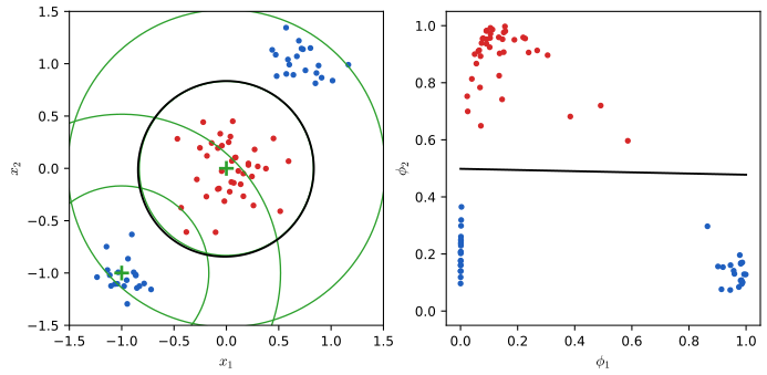
Fixed basis functions have serious limitations in high dimensions; later chapters let the network learn them.
5.4.3 Logistic regression
See also: companion course, Section 4.3.2, logistic regression (Result 4.12, 4.13) and Section 4.3.3, IRLS (Result 4.14); demo: logistic regression with IRLS.
pp. 159–161 The model is
\[ p(\cC{1}\given\bm\phi)=y(\bm\phi)=\sigma(\mathbf{w}^\T\bm\phi), \tag{5.71} \]with \(M\) parameters for \(M\) features, against \(2M+M(M+1)/2+1=M(M+5)/2+1\) for the Gaussian generative model (two means, a shared covariance, a prior). For \(t_n\in\{0,1\}\) and \(y_n=\sigma(a_n)\), \(a_n=\mathbf{w}^\T\bm\phi_n\), the likelihood and the cross-entropy error are
\[ p(\mathbf{t}\given\mathbf{w})=\prod_{n=1}^Ny_n^{t_n}\{1-y_n\}^{1-t_n},\qquad E(\mathbf{w})=-\ln p(\mathbf{t}\given\mathbf{w})=-\sum_{n=1}^N\{t_n\ln y_n+(1-t_n)\ln(1-y_n)\}. \tag{5.73, 5.74} \]Result 5.16 (gradient, Hessian and convexity of the cross-entropy; Exercise 5.19) p. 160, (5.72), (5.75)
\[ \frac{\d\sigma}{\d a}=\sigma(1-\sigma),\qquad \nabla E(\mathbf{w})=\sum_{n=1}^N(y_n-t_n)\bm\phi_n=\bm\Phi^\T(\mathbf{y}-\mathbf{t}),\qquad \nabla\nabla E(\mathbf{w})=\bm\Phi^\T\mathbf{R}\bm\Phi, \tag{5.72, 5.75} \]with \(\mathbf{R}=\diag(y_n(1-y_n))\). The Hessian is positive semi-definite, and positive definite when \(\bm\Phi\) has full column rank, so \(E\) is convex (strictly convex in the full-rank case): any stationary point is the global minimum, and Newton's method on it is the IRLS algorithm.
Proof
Per data point, \(\partial E/\partial y_n=-t_n/y_n+(1\)torch.autograd and the Hessian against finite differences; on random data IRLS converges in 5 steps to the point that 20000 steps of gradient descent reach. ∎
The gradient (5.75) has the same "error times input" form as the sum-of-squares gradient of linear regression (Section 4.1.3 of the book); Section 5.4.6 explains why. Each term \(\nabla E_n=(y_n-t_n)\bm\phi_n\) is what stochastic gradient descent uses.
Result 5.17 (maximum likelihood on separable data; Exercise 5.20) p. 161
Write \(\tilde t_n=2t_n-1\in\{-1,+1\}\). (a) If the data are linearly separable in feature space (some \(\hat{\mathbf{w}}\) has \(\tilde t_n\hat{\mathbf{w}}^\T\bm\phi_n\)
Proof
Each term of (5.74) equals \(\ln(1+e^{-\tilde t_na_n})\), which is positive for every finite \(a_n\). (a) Along \(\kappa\hat{\mathbf{w}}\), each term is \(\ln(1+e^{-\kappa c_n})\) with \(c_n\)
Filling the gap 5.10: what gradient descent does on separable data p. 161
The book says that the solution found "will depend on the choice of optimization algorithm". For batch gradient descent one can say exactly what happens to the error and the norm.
Derivation
The Hessian satisfies \(\bm\Phi^\T\mathbf{R}\bm\Phi\preceq\frac14\bm\Phi^\T\bm\Phi\), so \(\nabla E\) is Lipschitz with constant \(L=\frac14\|\bm\Phi\|_2^2\). For a convex \(L\)-smooth function and step \(\eta\le1/L\), the iterates \(\mathbf{w}_{t+1}=\mathbf{w}_t\)
(Proof: the descent lemma gives \(E(\mathbf{w}_{t+1})\le E(\mathbf{w}_t)\)
5.4.4 Multi-class logistic regression
See also: companion course, Section 4.3.4, multiclass logistic regression (Result 4.15).
pp. 161–162 With \(K\) classes,
\[ p(\cC{k}\given\bm\phi)=y_k(\bm\phi)=\frac{\exp(a_k)}{\sum_j\exp(a_j)},\qquad a_k=\mathbf{w}_k^\T\bm\phi, \tag{5.76, 5.77} \]and with 1-of-\(K\) targets the likelihood and the multi-class cross-entropy are
\[ p(\mathbf{T}\given\mathbf{w}_1,\dots,\mathbf{w}_K)=\prod_{n=1}^N\prod_{k=1}^Ky_{nk}^{t_{nk}},\qquad E(\mathbf{w}_1,\dots,\mathbf{w}_K)=-\sum_{n=1}^N\sum_{k=1}^Kt_{nk}\ln y_{nk}. \tag{5.79, 5.80} \]Result 5.18 (softmax derivatives and the multi-class gradient; Exercises 5.21, 5.22) p. 162, (5.78), (5.81), (5.82)
\[ \frac{\partial y_k}{\partial a_j}=y_k(I_{kj}-y_j),\qquad \nabla_{\mathbf{w}_j}E=\sum_{n=1}^N(y_{nj}-t_{nj})\bm\phi_n,\qquad \frac{\partial E}{\partial w_{ki}}=\sum_{n=1}^N(y_{nk}-t_{nk})\phi_i(\mathbf{x}_n), \tag{5.78, 5.81, 5.82} \]where \(w_{ki}\) is the weight from feature \(i\) to output \(k\). The Jacobian \(\mathbf{J}=\diag(\mathbf{y})\)
Proof
Jacobian. With \(Z=\sum_ie^{a_i}\): \(\partial y_k/\partial a_k=e^{a_k}/Z\)torch.autograd. ∎
5.4.5 Probit regression
See also: companion course, Section 4.3.5, probit regression (Filling the gap 4.7, the probit gradient and Hessian).
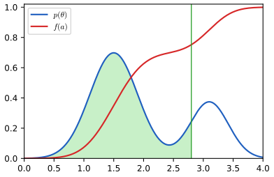
pp. 163–164 Other activation functions arise from a noisy threshold model: with \(a_n=\mathbf{w}^\T\bm\phi_n\), set \(t_n=1\) if \(a_n\ge\theta\) and \(t_n=0\) otherwise, where the threshold \(\theta\) is random with density \(p(\theta)\). Then
\[ p(t=1\given a)=f(a),\qquad f(a)=\int_{-\infty}^ap(\theta)\,\d\theta, \tag{5.83–5.85} \]and a standard normal threshold gives the probit function
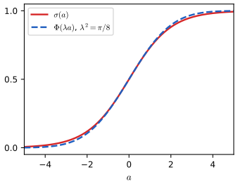
\[ \Phi(a)=\int_{-\infty}^a\N(\theta\given0,1)\,\d\theta. \tag{5.86} \]Result 5.19 (the threshold model, erf, and the probit approximation; Exercises 5.23, 5.24) pp. 163–164, (5.87), (5.88), Figure 5.12
- \(p(t=1\given a)=P(\theta\le a)=f(a)\), the distribution function of \(\theta\). A Gaussian threshold \(\N(m,s^2)\) gives \(\Phi((a-m)/s)\), which is the standard probit model with weights \(\mathbf{w}/s\) and the bias shifted by \(-m/s\): nothing new.
- With the book's definition \(\erf(a)\)
\({}=\frac2{\sqrt\pi}\int_0^a\exp(-\theta^2/2)\,\d\theta\) (5.87), \[ \Phi(a)=\frac12\Big\{1+\frac1{\sqrt2}\erf(a)\Big\}. \tag{5.88} \] The error function of numerical libraries has \(\exp(-\theta^2)\) in the integrand; with it, \(\Phi(a)=\tfrac12\{1+\erf(a/\sqrt2)\}\). The two are related by \(\erf_{\text{book}}(a)\) \({}=\sqrt2\,\erf(a/\sqrt2)\), so the book's version tends to \(\sqrt2\), not 1. - \(\Phi(\lambda a)\) and \(\sigma(a)\) have the same slope at \(a=0\) exactly when \(\lambda^2=\pi/8\); then \(\max_a|\sigma(a)-\Phi(\lambda a)|\)
\({}\approx0.018\).
Proof
(1) \(t=1\) if and only if \(\theta\le a\), and \(P(\theta\le a)\)
Filling the gap 5.11: tails, and why the probit model is less robust to mislabelled points p. 164
The book says the logistic tails decay like \(\exp(-x)\) and the probit tails "like \(\exp(-x^2)\)", hence the probit model "can be significantly more sensitive to outliers". The precise tail is \(e^{-x^2/2}/x\), and the mechanism is the size of the gradient.
Derivation
Tails. \(\sigma(-x)=1/(1+e^x)\sim e^{-x}\). For the normal tail with \(\varphi=\N(\cdot\given0,1)\) and \(x>0\): since \(u/x\ge1\) for \(u\ge x\) and \(u\varphi(u)=-\varphi'(u)\), \(1-\Phi(x)=\int_x^\infty\varphi\)
Influence of one mislabelled point. Take a point with \(t=1\) whose activation is \(a=-r\), \(r\) large (it lies far on the wrong side). Its error term and its derivative with respect to \(a\) are
\[ \text{logistic: } \ln(1+e^{r})\approx r,\quad \Big|\frac{\partial E_n}{\partial a}\Big|=\sigma(r)<1;\qquad \text{probit: } -\ln\Phi(-r)\approx\frac{r^2}2+\ln r,\quad \Big|\frac{\partial E_n}{\partial a}\Big|=\frac{\varphi(r)}{\Phi(-r)}\approx r. \]The last ratio, the inverse Mills ratio, lies between \(r\) and \(r+1/r\) by the tail bounds. So in the gradient \(\sum_n(\partial E_n/\partial a_n)\bm\phi_n\) the logistic model caps every point's weight at \(\|\bm\phi_n\|\), while the probit model lets a point's weight grow in proportion to how wrong it is: the fit is dragged towards the mislabelled point. A numerical computation confirms the ratio \(\varphi(r)/(r\Phi(-r))\to1\) and finds that one mislabelled point at \(x_1=10\) moves the probit boundary about nine times as far as the logistic one (0.20 against 0.02). ∎
Away from such points, probit and logistic fits are usually close: by Result 5.19(3) a probit weight vector is roughly \(\lambda=0.63\) times the logistic one.
5.4.6 Canonical link functions
See also: companion course, Section 4.3.6, canonical link functions (Results 4.16, 4.17).
pp. 164–165 Linear regression with Gaussian noise, logistic regression with the cross-entropy and softmax regression with the multi-class cross-entropy all have gradient "error \(y_n-t_n\) times feature \(\bm\phi_n\)". The reason is a matching of the activation function to an exponential-family distribution of the target,
\[ p(t\given\eta,s)=\frac1sh\Big(\frac ts\Big)g(\eta)\exp\Big\{\frac{\eta t}s\Big\}, \tag{5.89} \]with conditional mean \(y=\E[t\given\eta]\) related to \(\eta\) by \(\eta=\psi(y)\), and a generalised linear model \(y=f(\mathbf{w}^\T\bm\phi)\) (5.91) (Nelder and Wedderburn 1972).
Result 5.20 (the canonical link gives the error-times-feature gradient) pp. 164–165, (5.90)–(5.95)
- \(y\equiv\E[t\given\eta]=\)
\({}-s\frac{\d}{\d\eta}\ln g(\eta)\) (5.90), and \(\frac{\d y}{\d\eta}\) \({}=\var[t\given\eta]/s\ge0\), so \(\psi\) is increasing. - For \(N\) observations with a common \(s\), \(\ln p(\mathbf{t}\given\bm\eta,s)\)
\({}=\sum_n\{\ln g(\eta_n)+\eta_nt_n/s\}\) \({}+\const\) (5.92) and, with \(a_n=\mathbf{w}^\T\bm\phi_n\), \(y_n=f(a_n)\), \[ \nabla_{\mathbf{w}}\ln p(\mathbf{t}\given\bm\eta,s)=\sum_{n=1}^N\frac1s\{t_n-y_n\}\,\psi'(y_n)\,f'(a_n)\,\bm\phi_n. \tag{5.93} \] - If the activation is the inverse of \(\psi\), the canonical link \(f^{-1}(y)=\psi(y)\) (5.94), then \(\eta_n=a_n\), \(\psi'(y_n)f'(a_n)=1\), and for the error \(E=-\ln p\) \[ \nabla E(\mathbf{w})=\frac1s\sum_{n=1}^N\{y_n-t_n\}\bm\phi_n,\qquad \nabla\nabla E(\mathbf{w})=\frac1{s}\sum_{n=1}^Nf'(a_n)\bm\phi_n\bm\phi_n^\T\succeq0. \tag{5.95} \] So with the canonical link the negative log likelihood is always convex. (The book's (5.95) writes \(\nabla\ln E\); the gradient of \(E\) is meant.)
Proof
(1) Normalisation: \(g(\eta)\int\frac1sh(t/s)e^{\eta t/s}\d t\)
The pairing of output activation and error function (identity with sum of squares, sigmoid with binary cross-entropy, softmax with multi-class cross-entropy) carries over unchanged to the output layer of the deep networks of the following chapters, where the output "delta" \(y_n-t_n\) starts backpropagation.
Exercises
Each exercise is restated in my own words with the book's number and difficulty; the solutions are my own, compared afterwards with the official solutions manual. Where a solution there has a slip, a short note says so (see also Corrections). "Companion" links point to the same exercise in Bishop (2006).
Exercise 5.1 (★). With 1-of-\(K\) targets, show that \(\E[\mathbf{t}\given\mathbf{x}]\) is the vector of posterior probabilities.
Solution
\(t_k\in\{0,1\}\) and \(t_k=1\) exactly when the class is \(\cC{k}\), so \(\E[t_k\given\mathbf{x}]=P(t_k\)
\({}=1\given\mathbf{x})\) \({}=p(\cC{k}\given\mathbf{x})\). See Result 5.3. (Agrees with the manual.) Exercise 5.2 (★★). The convex hull of \(\{\mathbf{x}_n\}\) is the set of all \(\sum_n\alpha_n\mathbf{x}_n\) with \(\alpha_n\ge0\), \(\sum_n\alpha_n=1\). Two point sets are linearly separable if some \(\hat{\mathbf{w}},w_0\) have \(\hat{\mathbf{w}}^\T\mathbf{x}_n+w_0\)
\({}>0\) for all \(\mathbf{x}_n\) and \(\hat{\mathbf{w}}^\T\mathbf{y}_m+w_0\) \({}<0\) for all \(\mathbf{y}_m\). Show that intersecting hulls rule out separability, and that separable sets have disjoint hulls. (Companion: Exercise 4.1.) Solution
Suppose \(\mathbf{z}=\sum_n\alpha_n\mathbf{x}_n\)
\({}=\sum_m\beta_m\mathbf{y}_m\) lies in both hulls and \((\hat{\mathbf{w}},w_0)\) separates. Because the weights sum to one, \(\hat{\mathbf{w}}^\T\mathbf{z}+w_0\) \({}=\sum_n\alpha_n(\hat{\mathbf{w}}^\T\mathbf{x}_n\) \({}+w_0)>0\) (a convex combination of positive numbers, with at least one \(\alpha_n>0\)), and by the same computation with the \(\mathbf{y}_m\), \(\hat{\mathbf{w}}^\T\mathbf{z}+w_0<0\): a contradiction. The second statement is the contrapositive of the first, so there is nothing more to prove. (For finite sets the converse also holds, disjoint hulls imply separability, by the separating hyperplane theorem for disjoint compact convex sets.) The manual's argument is the same; its (131) writes \(\mathbf{y}_m\) where \(\mathbf{x}_n\) is meant. Exercise 5.3 (★★). If every target row satisfies \(\mathbf{a}^\T\mathbf{t}_n+b=0\), show that the least-squares prediction (5.16) satisfies \(\mathbf{a}^\T\mathbf{y}(\mathbf{x})+b\)
\({}=0\) for every \(\mathbf{x}\), assuming a constant basis function \(\phi_0=1\). (Companion: Exercise 4.2.) Solution
Result 5.4 with a single constraint: \(\mathbf{T}\mathbf{a}=-b\one_N=\)
\({}-b\widetilde{\mathbf{X}}\mathbf{e}_1\), so \(\mathbf{a}^\T\mathbf{y}(\mathbf{x})\) \({}=\tilde{\mathbf{x}}^\T\widetilde{\mathbf{X}}^\dagger\mathbf{T}\mathbf{a}\) \({}=-b\,\tilde{\mathbf{x}}^\T\mathbf{e}_1\) \({}=-b\). The manual instead eliminates the bias, centres the data and works with the centred pseudo-inverse; both are correct. In its derivative (134) the factor 2 is spurious (the error carries a \(\tfrac12\)); it does not affect the solution. Exercise 5.4 (★★). Extend Exercise 5.3 to several simultaneous linear constraints. (Companion: Exercise 4.3.)
Solution
Stack the constraints as \(\mathbf{A}\mathbf{t}_n+\mathbf{b}\)
\({}=\mathbf{0}\); the computation in Result 5.4 is written for this matrix case and gives \(\mathbf{A}\mathbf{y}(\mathbf{x})\) \({}+\mathbf{b}=\mathbf{0}\). Checked numerically with two random constraints (residual \(10^{-14}\)). (Agrees with the manual.) Exercise 5.5 (★). From (5.38), (5.30), (5.31), derive (5.39).
Solution
See Result 5.8: \(1/P+1/R=(2N_\mathrm{TP}+N_\mathrm{FP}\)
\({}+N_\mathrm{FN})/N_\mathrm{TP}\) and \(F=2/(1/P+1/R)\). (Agrees with the manual, which multiplies out instead.) Exercise 5.6 (★★). Show that \(0\le a\le b\) implies \(a\le(ab)^{1/2}\), and deduce that the minimum-error rule has \(p(\text{mistake})\)
\({}\le\int\{p(\mathbf{x},\cC{1})p(\mathbf{x},\cC{2})\}^{1/2}\d\mathbf{x}\) (5.99). (Companion: Exercise 1.21.) Solution
Multiply \(\sqrt a\le\sqrt b\) by \(\sqrt a\ge0\). For the minimum-error rule, by Result 5.5, \(p(\text{mistake})\)
\({}=\int\min\{j_1,j_2\}\d\mathbf{x}\) with \(j_k=p(\mathbf{x},\cC{k})\), and \(\min\{j_1,j_2\}\le\sqrt{j_1j_2}\) pointwise by the first part (with \(a\) the smaller, \(b\) the larger). This Bhattacharyya-type bound is 0.377 against the true 0.227 for the demo's problem with \(d=1.5\). (Agrees with the manual, whose reference "(??)" is a broken cross-reference to (5.20).) Exercise 5.7 (★). Show that \(L_{kj}=1-I_{kj}\) turns the minimum-expected-loss rule into the largest-posterior rule, and interpret this loss. (Companion: Exercise 1.22.)
Solution
\(\sum_k(1\)
\({}-I_{kj})p(\cC{k}\given\mathbf{x})=1\) \({}-p(\cC{j}\given\mathbf{x})\), minimised by the largest posterior. The loss counts one per mistake and nothing for a correct decision, so its expectation is the misclassification rate. (Agrees with the manual.) Exercise 5.8 (★). Give the minimum-expected-loss criterion for a general loss matrix and general priors. (Companion: Exercise 1.23.)
Solution
Assign \(\mathbf{x}\) to \(\argmin_j\sum_kL_{kj}p(\mathbf{x}\given\cC{k})p(\cC{k})\), which is (5.23) multiplied by \(p(\mathbf{x})>0\). For two classes with zero diagonal: decide \(\cC{2}\) when \(p(\mathbf{x}\given\cC{2})/p(\mathbf{x}\given\cC{1})\)
\({}\ge L_{12}p(\cC{1})/(L_{21}p(\cC{2}))\): the loss ratio and the prior ratio enter only through their product. (Agrees with the manual.) Exercise 5.9 (★). Show that \(\frac1N\sum_{n=1}^Np(\cC{k}\given\mathbf{x}_n)\) tends to \(p(\cC{k})\) as \(N\to\infty\). (The book's sum index is misprinted as \(N=1\).)
Solution
If the \(\mathbf{x}_n\) are independent draws from \(p(\mathbf{x})\), the strong law of large numbers gives convergence (almost surely) to \(\E[p(\cC{k}\given\mathbf{x})]\)
\({}=\int p(\cC{k}\given\mathbf{x})p(\mathbf{x})\d\mathbf{x}\) \({}=\int p(\mathbf{x},\cC{k})\d\mathbf{x}\) \({}=p(\cC{k})\); the summands lie in \([0,1]\), so the expectation exists. Monte Carlo with 400000 draws gives 0.3001 for \(p(\cC{2})=0.3\). The assumption that the \(\mathbf{x}_n\) come from the same distribution as the training data matters: this is the basis of a simple check for prior shift. (Agrees with the manual.) Exercise 5.10 (★★). With loss matrix \(L_{kj}\) and a loss \(\lambda\) for rejecting, find the minimum-expected-loss decision, check that it reduces to the reject rule of Section 5.2.3 for \(L_{kj}=1-I_{kj}\), and relate \(\lambda\) to \(\theta\). (Companion: Exercise 1.24.)
Solution
Result 5.7(b), (c): decide \(\argmin_jr_j(\mathbf{x})\) if \(\min_jr_j(\mathbf{x})<\lambda\), otherwise reject; for 0–1 loss this is "reject if \(\max_kp(\cC{k}\given\mathbf{x})\le1\)
\({}-\lambda\)", so \(\theta=1-\lambda\). Rejecting never pays if \(\lambda\ge1-1/K\) (every input is then decided) and always if \(\lambda=0\). (Agrees with the manual.) Exercise 5.11 (★). Show \(\sigma(-a)=1-\sigma(a)\) and \(\sigma^{-1}(y)=\ln\{y/(1-y)\}\). (Companion: Exercise 4.7.)
Solution
Result 5.10(1). (Agrees with the manual.)
Exercise 5.12 (★). Derive (5.48) with (5.49), (5.50) from (5.40), (5.41) for Gaussian classes with a shared covariance. (Companion: Exercise 4.8.)
Solution
Result 5.11. The manual reaches the same result, but its intermediate lines drop the inverse on \(\bm\Sigma\) (they show \(\mathbf{x}\bm\Sigma^\T\mathbf{x}\), \(\bm\mu_1^\T\bm\Sigma\bm\mu_1\) and \(\bm\mu_2^\T\bm\Sigma\bm\mu_2\) where \(\bm\Sigma^{-1}\) is meant).
Exercise 5.13 (★). A generative model has priors \(\pi_k\) and any class densities \(p(\bm\phi\given\cC{k})\). For independent labelled data with 1-of-\(K\) targets, show that the maximum-likelihood priors are \(\pi_k=N_k/N\) (5.101). (Companion: Exercise 4.9.)
Solution
The log likelihood is \(\sum_n\sum_kt_{nk}\{\ln p(\bm\phi_n\given\cC{k})\)
\({}+\ln\pi_k\}\); only \(\sum_kN_k\ln\pi_k\) depends on the priors. Lagrange (or Gibbs' inequality) as in Result 5.12 gives \(\pi_k=N_k/N\), whatever the class densities. (Agrees with the manual.) Exercise 5.14 (★★). With Gaussian class densities \(\N(\bm\phi\given\bm\mu_k,\bm\Sigma)\) sharing \(\bm\Sigma\), show that the maximum-likelihood means are the class means (5.103) and that \(\bm\Sigma=\sum_k(N_k/N)\mathbf{S}_k\) (5.104), (5.105). (Companion: Exercise 4.10.)
Solution
Result 5.12, where the covariance step is done in the precision \(\bm\Lambda=\bm\Sigma^{-1}\), in which the objective is concave, so the stationary point is the maximum. The manual's version has typos in (154) (\((\bm\phi-\bm\mu)\) for \((\bm\phi_n-\bm\mu_k)\)) and (157) (a sum written \(\sum^T_k\), and \(\bm\mu_n\) for \(\bm\mu_k\)); the result is right.
Exercise 5.15 (★★). Find the maximum-likelihood \(\mu_{ki}\) for the binary naive Bayes model of Section 5.3.3.
Solution
Result 5.13(b): \(\mu_{ki}\)
\({}=\frac1{N_k}\sum_{n\in\cC{k}}x_{ni}\), the fraction of class-\(k\) points with \(x_i=1\). The manual's (160) writes \(\frac1N\sum_{n=1}^N x_{ni}\), reusing \(N\) for the number of points in class \(k\) and summing over those points only; read literally (all \(N\) points) it would give the same estimate for every class. Exercise 5.16 (★★). \(M\) features with \(L\) states each, coded 1-of-\(L\), independent given the class: show that the activations \(a_k\) of (5.46) are linear in the codes. (Companion: Exercise 4.11.)
Solution
Result 5.13(c): \(a_k=\sum_{m,l}\phi_{ml}\ln\mu_{kml}\)
\({}+\ln p(\cC{k})\). (Agrees with the manual.) Exercise 5.17 (★★). Find the maximum-likelihood parameters of the model of Exercise 5.16.
Solution
Result 5.13(c): \(\mu_{kml}=N_{kml}/N_k\), with one Lagrange multiplier per (class, feature) pair. The manual writes the denominator as \(\sum_n\sum_l\phi_{nml}\), which is \(N_k\) because each point has exactly one active state per feature; its sums run over the points of class \(k\).
Exercise 5.18 (★). Verify \(\d\sigma/\d a=\sigma(1-\sigma)\) (5.72). (Companion: Exercise 4.12.)
Solution
Result 5.10(1). (Agrees with the manual.)
Exercise 5.19 (★). Use (5.72) to show that the gradient of (5.74) is (5.75). (Companion: Exercise 4.13.)
Solution
Result 5.16. (Agrees with the manual.)
Exercise 5.20 (★). Show that for linearly separable data the maximum-likelihood logistic regression solution is obtained by a separating \(\mathbf{w}\) with \(\|\mathbf{w}\|\to\infty\). (Companion: Exercise 4.14.)
Solution
Result 5.17: the likelihood approaches its supremum 1 along \(\kappa\hat{\mathbf{w}}\), \(\kappa\to\infty\), for any strictly separating \(\hat{\mathbf{w}}\), and is not attained; strictly speaking there is no maximum-likelihood solution, only a maximising sequence. The manual's argument uses "\(\mathbf{w}^\T\bm\phi_n\ge0\) if \(t_n=1\)", which allows points on the boundary; such a point keeps \(y_n=\tfrac12\) for every \(\kappa\), so the separation must be strict.
Exercise 5.21 (★). Show that the softmax derivatives are (5.78). (Companion: Exercise 4.17.)
Solution
Result 5.18. (Agrees with the manual.)
Exercise 5.22 (★). Using (5.78), show that the gradients of (5.80) are (5.81). (Companion: Exercise 4.18.)
Solution
Result 5.18; the step that needs \(\sum_kt_{nk}=1\) is \(\partial E_n/\partial a_{nj}=y_{nj}\)
\({}-t_{nj}\). (Agrees with the manual.) Exercise 5.23 (★). Show that the probit function (5.86) and the erf function (5.87) are related by (5.88). (Companion: Exercise 4.21.)
Solution
Result 5.19(2): with the book's (5.87), \(\Phi(a)=\tfrac12\)
\({}+\frac1{\sqrt{2\pi}}\int_0^ae^{-\theta^2/2}\d\theta\) \({}=\tfrac12\{1+\erf(a)/\sqrt2\}\), which is (5.88) directly, no substitution needed. The manual's solution substitutes \(\theta=\sqrt2u\) and obtains \(\Phi(a)=\tfrac12\{1+\erf(a/\sqrt2)\}\) "using (5.87)"; that step uses the library definition \(\erf(z)\) \({}=\frac2{\sqrt\pi}\int_0^ze^{-u^2}\d u\), not (5.87), and under the book's own definition \(\tfrac12\{1+\erf(a/\sqrt2)\}\ne\Phi(a)\) (at \(a=1\): 0.868 against 0.841). Both final formulas are right in their own convention; the manual mixes the two. Verified numerically. Exercise 5.24 (★★). Approximating \(\sigma(a)\) by \(\Phi(\lambda a)\) with equal derivatives at \(a=0\), show \(\lambda^2=\pi/8\). (Companion: Exercise 4.25.)
Solution
Result 5.19(3): \(\tfrac14=\lambda/\sqrt{2\pi}\). (Agrees with the manual.)
Corrections to the book and the solutions manual
Found while writing these notes; each is checked either by direct algebra or numerically.
Book (first edition, 2024).
- p. 139: "\(p(\cC{1})\) represents the probability that a person has cancer": the same page defines \(\cC{1}\) as the absence of cancer, so this is \(p(\cC{2})\) (and likewise \(p(\cC{2}\given\mathbf{x})\) in the next sentence).
- p. 149: the F-score is called "the geometric mean of precision and recall"; (5.38) is the harmonic mean, which differs (Result 5.8).
- (5.66)–(5.68): the factor \(1/s\) is missing in front of \(\bm\lambda^\T\mathbf{x}\) in (5.67) and (5.68), and the prefactor of (5.66) should be \(1/s^D\) for \(\mathbf{x}\in\R^D\) (Result 5.14; numerically the printed log odds are wrong by more than 0.5 for \(s=2\)).
- (5.70) is misprinted as \(f(\mathbf{w}^\T\mathbf{w}+w+0)\); it should be \(f(\mathbf{w}^\T\mathbf{x}+w_0)\).
- Figure 5.16 caption: the outputs are \(y_1,\dots,y_K\), not \(y_1,\dots,y_N\).
- (5.82): the left side should be \(\partial E/\partial w_{ki}\) (or the right side should use \(j\)); the text's "output unit \(t_k\)" means \(y_k\).
- (5.87): the integrand \(\exp(-\theta^2/2)\) does not define the erf that "many numerical packages" evaluate (\(\exp(-\theta^2)\)). With the printed definition (5.88) is correct; with the library erf the relation is \(\Phi(a)=\tfrac12\{1+\erf(a/\sqrt2)\}\).
- p. 164: the probit tail decays like \(\exp(-x^2/2)/x\), not \(\exp(-x^2)\) (Filling the gap 5.11); the conclusion about outliers stands.
- (5.95): "\(\nabla\ln E(\mathbf{w})\)" should be \(\nabla E(\mathbf{w})\).
- Exercise 5.9: the summation index is printed as \(N=1\); it should be \(n=1\).
Solutions manual (version 1.0).
- 5.2: in (131) the last sum has \(\mathbf{y}_m\) where \(\mathbf{x}_n\) is meant.
- 5.3: the derivative (134) has a spurious factor 2; harmless, since it is set to zero.
- 5.6: the reference to (5.20) is printed as "(??)".
- 5.12: intermediate lines omit the inverse on \(\bm\Sigma\); the final result is right.
- 5.14: index typos in (154) and (157); the result is right.
- 5.15: (160) normalises by \(N\) and sums over \(n=1,\dots,N\), meaning the \(N_k\) points of class \(k\); as printed it reads like the overall mean.
- 5.20: uses \(\mathbf{w}^\T\bm\phi_n\ge0\) where strict separation is needed, and calls the limit a maximum, which is not attained.
- 5.23: claims to use (5.87) but uses the library definition of erf, reaching a formula that differs from (5.88) under the book's definition (see Exercise 5.23).
Demonstrations for this chapter
Each demonstration runs in the browser and links back to these notes; the ▶ Demo boxes above open them already set to the case under discussion. The Python code computes the same numbers: the decision-theory quantities, the generative fits and the training errors after 100 gradient steps agree with the pages to about \(10^{-14}\).
| Demonstration | What you can see | Sections |
|---|---|---|
| Decision theory: the loss matrix, the reject option and the ROC curve | A one-dimensional screening problem: joint densities with the false positives and false negatives shaded, the posteriors with the threshold and the reject band, the ROC curve with the operating point, the expected loss against the threshold, and the confusion matrix with precision, recall and F-score. Presets: 1 minimum misclassification rate (Fig. 5.5); 2 a missed cancer costs 100 (Fig. 5.6); 3 reject option (Fig. 5.7); 4 rare disease, accuracy misleads; 5 a far mode that does not matter (Fig. 5.8). | 5.2.1–5.2.6 (Results 5.5–5.9) |
| Generative classifiers: Gaussian classes, linear and quadratic boundaries | Two or three Gaussian classes: the density ellipses, the posterior as a colour mix with the decision boundaries, shared or different covariances, the prior slider and the maximum-likelihood fit from a sample. Presets: 1 shared covariance (Fig. 5.13); 2 a prior shifts the boundary in parallel; 3 three classes (Fig. 5.14); 4 quadratic boundaries; 5 maximum-likelihood fit. | 5.3, 5.3.1, 5.3.2 (Results 5.11, 5.12) |
| Training single-layer classifiers: least squares, logistic, probit and softmax | Gradient descent from w = 0 with hand-written forward and backward passes: the probability map and boundaries, the error and the weight norm against the iteration, least squares for comparison, weight decay and Gaussian basis functions. Presets: 1 far points (Fig. 5.4); 2 separable data; 3 softmax for three classes; 4 basis functions (Fig. 5.15); 5 probit against logistic. | 5.1.4, 5.4.2–5.4.5 (Results 5.16–5.19) |
The Python code that makes every figure on this page is code/ch05_single_layer_classification.py (see the code index). In the companion course: decision theory, least squares, Fisher and the perceptron, logistic regression with IRLS and the Laplace approximation.
References
- Bishop, C. M. and Bishop, H. (2024). Deep Learning: Foundations and Concepts. Springer, Cham. Chapter 5, pp. 131–169. doi:10.1007/978-3-031-45468-4. Book website: www.bishopbook.com.
- Bishop, C. M. and Bishop, H. (2024). Deep Learning: Foundations and Concepts. Solutions to the Exercises, version 1.0 (Chapters 2–10).
- Bishop, C. M. (2006). Pattern Recognition and Machine Learning. Springer, New York. Sections 1.5 and 4.1–4.3 (and the official errata).
- Berger, J. O. (1985). Statistical Decision Theory and Bayesian Analysis, 2nd ed. Springer, New York.
- Duda, R. O. and Hart, P. E. (1973). Pattern Classification and Scene Analysis. Wiley, New York.
- Fawcett, T. (2006). An introduction to ROC analysis. Pattern Recognition Letters, 27(8), 861–874. doi:10.1016/j.patrec.2005.10.010.
- Hanley, J. A. and McNeil, B. J. (1982). The meaning and use of the area under a receiver operating characteristic (ROC) curve. Radiology, 143(1), 29–36.
- McCullagh, P. and Nelder, J. A. (1989). Generalized Linear Models, 2nd ed. Chapman and Hall, London.
- Nelder, J. A. and Wedderburn, R. W. M. (1972). Generalized linear models. Journal of the Royal Statistical Society, Series A, 135(3), 370–384.
- Nesterov, Y. (2004). Introductory Lectures on Convex Optimization: A Basic Course. Kluwer, Boston. (The convergence bound used in Filling the gap 5.10.)
- Neyman, J. and Pearson, E. S. (1933). On the problem of the most efficient tests of statistical hypotheses. Philosophical Transactions of the Royal Society of London, Series A, 231, 289–337.
All numerical statements in the text (gradients against finite differences and torch.autograd, the decision-theory integrals, the convergence and separability claims, and the corrections) were confirmed numerically.