Multivariate Models
Most data sets record several variables on each unit, and the interesting questions are about how the variables move together. This chapter collects the basic models for such data: random vectors with their mean vector and covariance matrix; the correlation between two variables, estimated with an interval built on Fisher's variance-stabilising transformation; the multivariate normal, with its maximum likelihood estimators; and the multinomial, the model for counts in several categories. The book's treatment is brief and states almost everything without proof. These notes prove it all, and add the results that make the chapter usable: the sampling distribution of the correlation and why its standard error is \(1/\sqrt{n-3}\), conditioning a normal vector, the joint distribution of the sample mean and covariance (the Wishart distribution), Hotelling's \(T^2\) test, and the Fisher information of the multinomial.
Ch. 1 Probability Ch. 2 Random variables Ch. 3 Expectation Ch. 4 Inequalities Ch. 5 Convergence Ch. 6 Models and inference Ch. 7 Estimating the CDF Ch. 8 Bootstrap Ch. 9 Parametric inference Ch. 10 Hypothesis testing Ch. 11 Bayesian inference Ch. 12 Decision theory Ch. 13 Regression Ch. 14 Multivariate models Ch. 15 Independence Ch. 16 Causal inference Ch. 17 Directed graphs Ch. 18 Undirected graphs Ch. 19 Log-linear models Ch. 20 Curve estimation Ch. 21 Orthogonal functions Ch. 22 Classification Ch. 23 Stochastic processes Ch. 24 Simulation
How to read these notes
They follow the book. Sections carry the book's numbers (14.1 to 14.7), Theorems 14.1 to 14.6 keep the book's numbers, and every displayed equation that appears in the book carries the book's own equation number, e.g. \((14.8)\). Results added here are numbered from 14.7 on and marked as additions.
Filling the gaps. Of the chapter's six theorems the book proves two (the multinomial covariance and its MLE) and part of a third (the normal log-likelihood, in the appendix); the rest, the facts about traces and square roots, the unbiasedness of \(\bS\), the standard error of Fisher's \(z\) and the multinomial limit theorem, are stated. Each gets a complete argument here, in an orange Filling the gap box or a proof; they start hidden: open one with its bar, or use the button below.
Figures and demonstrations. The chapter has no figures of its own. The six figures here are supplementary (numbered 14.S1 to 14.S6): they illustrate the results proved in the notes and answer the computer exercises, and are made by the Python code. The ▶ Demo boxes open an interactive demonstration already set to the case being discussed.
Main reference
L. Wasserman, All of Statistics: A Concise Course in Statistical Inference, Springer (2004), Chapter 14, pages 231–238 (book website: www.stat.cmu.edu/~larry/all-of-statistics). Section, theorem, equation and exercise numbers below refer to this book. Further reading is listed in the references.
The explanations, derivations, figures and code are my own; equations are cited by their numbers in the book.
Companion courses
Much of this chapter appears elsewhere on this site:
- The multivariate normal (its density, linear maps, margins, conditionals and the \(\chi^2\) quadratic form) is proved in full earlier in this course: Chapter 2, Result 2.15 and Result 2.16; Chapter 3, Definition 3.6 (mean vector and covariance matrix) and Filling the gap 3.7. The multinomial: Result 2.14, Filling the gap 3.6, and Pearson's \(\chi^2\) test in Theorem 10.17.
- Bayesian and Probabilistic Machine Learning, Chapter 2: the Gaussian distribution (conditional and marginal Gaussians in Result 2.9, maximum likelihood and its bias in Result 2.14), the multinomial; and the mathematical toolkit for trace identities, the determinant lemma and the Wishart distribution.
- Foundations of Deep Learning, Chapter 3: the multivariate Gaussian (conditioning by completing the square, Result 3.7; the Schur complement, Result 3.8; maximum likelihood with a calculus proof that it is the global maximum, Filling the gap 3.4) and the multinomial, with why it needs \(k-1\) parameters.
- Statistical Methods for Modern Biology, Chapter 7: covariance and correlation as matrix operations, what changes of units do to them, and why nearly equal sample eigenvalues are unstable.
Where a proof there is the same, these notes give it briefly and link to it. New here: the asymptotic distribution of the sample correlation for any distribution with four moments, the proof that Fisher's \(z\) is variance stabilising and that \(n-3\) is right to second order, conditioning a normal vector on an arbitrary linear combination, a matrix-calculus-free proof that the MLE of \(\bSigma\) is the global maximum, the joint law of \(\Xbar\) and \(\bS\), Hotelling's \(T^2\) with the proof of its \(F\) distribution, and the Fisher information of the multinomial.
The chapter at a glance
- Random vectors (Theorem 14.1): \(\E(\bA\bX)=\bA\bmu\), \(\V(\bA\bX)=\bA\bSigma\bA^\T\); covariance matrices are symmetric and positive semidefinite (gap 14.2); \(\E(\bS)=\bSigma\) (gap 14.3).
- The correlation (Section 14.2): \(\sqrt n(\hrho-\rho)\) is asymptotically \(\N(0,(1-\rho^2)^2)\) for normal data (gap 14.5); \(z=\artanh\hrho\) removes the dependence on \(\rho\) (gap 14.6); \(\V(z)=1/(n-3)\) to second order (gap 14.7), but only for normal data.
- The multivariate normal (Section 14.3): conditioning on \(\ba^\T\bX=c\) (gap 14.9); the MLE \((\Xbar,\tfrac{n-1}n\bS)\) is the unique global maximum when \(n\gt k\) and does not exist otherwise (gap 14.10); \(\Xbar\sim\N(\bmu,\bSigma/n)\) independent of \((n-1)\bS\sim\Wish_k(n-1,\bSigma)\) (gap 14.11); Hotelling's \(T^2\) has an exact \(F\) law (Result 14.7), is the likelihood ratio test and the largest squared t-statistic over all linear combinations (gap 14.13).
- The multinomial (Section 14.4): \(\V(\bX)=n(\diag\bp-\bp\bp^\T)\), singular (Theorem 14.4); \(\hp=\bX/n\) is the global maximum (gap 14.16) and attains the Cramér–Rao bound (gap 14.17); \(\sqrt n(\hp-\bp)\) tends to a singular normal law, which gives Pearson's \(\chi^2_{k-1}\) (gap 14.18).
Notation. Vectors and matrices are bold: \(\bX=(X_1,\dots,X_k)^\T\) is a random vector, \(\bmu=\E(\bX)\), \(\bSigma=\V(\bX)\). A sample is \(\bX_1,\dots,\bX_n\) (the book writes \(X_{ij}\) for coordinate \(i\) of observation \(j\)); \(\Xbar=n^{-1}\sum_i\bX_i\), \(\bS\) is the sample covariance matrix with divisor \(n-1\), (14.4), and \(\hSigma=\frac{n-1}n\bS\) the one with divisor \(n\). \(\bI\) is the identity, \(\bone\) the vector of ones, \(\be_j\) the \(j\)-th unit vector, \(|\bA|\) the determinant. \(\N(\bmu,\bSigma)\) is the \(k\)-dimensional normal distribution, \(\chi^2_m\) the chi-squared distribution with \(m\) degrees of freedom, \(z_{\alpha/2}\) the upper \(\alpha/2\) quantile of \(\N(0,1)\). Logarithms are natural.
Prerequisites. Expectation and covariance (Chapter 3), the multivariate central limit theorem and delta method (Chapter 5, Theorem 5.12 and Theorem 5.15), maximum likelihood and Fisher information (Chapter 9), the bootstrap (Chapter 8).
Linear algebra notation
p. 231 The chapter opens with a table of notation: the inner product \(\bx^\T\by=\sum_jx_jy_j\), the determinant \(|\bA|\), the transpose \(\bA^\T\), the inverse \(\bA^{-1}\), the identity \(\bI\), the trace \(\tr(\bA)=\sum_ia_{ii}\) of a square matrix, and the square root \(\bA^{1/2}\) of a symmetric positive definite matrix. A symmetric matrix \(\bSigma\) is positive definite if \(\bx^\T\bSigma\bx\gt0\) for every \(\bx\ne\bzero\), and positive semidefinite if \(\bx^\T\bSigma\bx\ge0\) for every \(\bx\). Two facts carry the whole chapter: the trace lets us move a quadratic form into a product of matrices, and the square root lets us turn any normal vector into a vector of independent standard normals.
Filling the gap 14.1: the trace identities, and the square root of a positive definite matrix p. 231
(a) For an \(m\times k\) matrix \(\bA\) and a \(k\times m\) matrix \(\bB\), \(\tr(\bA\bB)=\tr(\bB\bA)\); for square \(\bA,\bB\) of the same size, \(\tr(\bA+\bB)=\tr(\bA)+\tr(\bB)\) and \(\tr(c\bA)=c\tr(\bA)\); for a scalar, \(\tr(a)=a\). In particular, for a vector \(\bx\) and square \(\bA\),
\[ \bx^\T\bA\bx=\tr(\bx^\T\bA\bx)=\tr(\bA\bx\bx^\T). \](b) If \(\bA\) is symmetric and positive definite, there is exactly one symmetric positive definite matrix \(\bA^{1/2}\) with \(\bA^{1/2}\bA^{1/2}=\bA\); it satisfies (1) \(\bA^{1/2}\) is symmetric, (2) \(\bA=\bA^{1/2}\bA^{1/2}\), (3) \(\bA^{1/2}\bA^{-1/2}\)\({}=\bA^{-1/2}\bA^{1/2}\)\({}=\bI\) with \(\bA^{-1/2}=(\bA^{1/2})^{-1}\), and moreover \(\bA^{-1/2}=(\bA^{-1})^{1/2}\) and \(|\bA^{1/2}|=|\bA|^{1/2}\).
Derivation
(a) \(\tr(\bA\bB)\)\({}=\sum_{i=1}^m(\bA\bB)_{ii}\)\({}=\sum_{i=1}^m\sum_{j=1}^ka_{ij}b_{ji}\)\({}=\sum_{j=1}^k\sum_{i=1}^mb_{ji}a_{ij}\)\({}=\sum_{j=1}^k(\bB\bA)_{jj}\)\({}=\tr(\bB\bA)\): the two finite sums may be exchanged. Linearity is immediate from \(\tr(\bA)=\sum_ia_{ii}\). Applying (a) with the \(1\times k\) matrix \(\bx^\T\) and the \(k\times1\) matrix \(\bA\bx\) gives \(\tr(\bx^\T\bA\bx)=\tr(\bA\bx\bx^\T)\). Applied twice, it gives the cyclic rule \(\tr(\bA\bB\bm{C})=\tr(\bm{C}\bA\bB)\); arbitrary permutations are not allowed.
(b) Existence. By the spectral theorem a real symmetric matrix can be written \(\bA=\bm{U}\bLambda\bm{U}^\T\), with \(\bm{U}\) orthogonal (\(\bm{U}^\T\bm{U}=\bm{U}\bm{U}^\T=\bI\), columns \(\bu_i\)) and \(\bLambda\)\({}=\diag(\lambda_1,\dots,\lambda_k)\). Then \(\bx^\T\bA\bx\)\({}=\sum_i\lambda_i(\bu_i^\T\bx)^2\), and choosing \(\bx=\bu_i\) shows that \(\bA\) is positive definite if and only if every \(\lambda_i\gt0\). Define \(\bA^{1/2}=\bm{U}\bLambda^{1/2}\bm{U}^\T\) with \(\bLambda^{1/2}=\diag(\sqrt{\lambda_i})\). It is symmetric, positive definite (its eigenvalues are \(\sqrt{\lambda_i}\gt0\)), and \(\bA^{1/2}\bA^{1/2}\)\({}=\bm{U}\bLambda^{1/2}\bm{U}^\T\bm{U}\bLambda^{1/2}\bm{U}^\T\)\({}=\bm{U}\bLambda\bm{U}^\T\)\({}=\bA\). Its inverse is \(\bm{U}\bLambda^{-1/2}\bm{U}^\T\) (multiply out), which is also the square root of \(\bA^{-1}=\bm{U}\bLambda^{-1}\bm{U}^\T\); so (3) holds, and \(|\bA^{1/2}|\)\({}=\prod_i\sqrt{\lambda_i}\)\({}=|\bA|^{1/2}\).
Uniqueness. Let \(\bm{R}\) be symmetric positive definite with \(\bm{R}^2=\bA\). Then \(\bm{R}\bA=\bm{R}^3=\bA\bm{R}\), so \(\bm{R}\) maps each eigenspace \(E_\lambda=\{\bx:\bA\bx=\lambda\bx\}\) into itself (if \(\bA\bx=\lambda\bx\) then \(\bA\bm{R}\bx\)\({}=\bm{R}\bA\bx\)\({}=\lambda\bm{R}\bx\)). Restricted to \(E_\lambda\), \(\bm{R}\) is symmetric with \(\bm{R}^2=\lambda\bI\), so its eigenvalues there are \(\pm\sqrt\lambda\), and positive definiteness leaves only \(+\sqrt\lambda\): \(\bm{R}=\sqrt\lambda\,\bI\) on \(E_\lambda\). The eigenspaces span \(\R^k\), so \(\bm{R}\) agrees with \(\bA^{1/2}\) everywhere. ∎
Other "square roots" exist if symmetry is dropped: the Cholesky factor \(\bm{L}\) (lower triangular, \(\bm{L}\bm{L}^\T=\bA\)) is the one used in practice to simulate normal vectors (Exercise 4). Everything below that uses \(\bSigma^{1/2}\) only needs some \(\bB\) with \(\bB\bB^\T=\bSigma\).
14.1 Random Vectors
p. 232 A random vector \(\bX=(X_1,\dots,X_k)^\T\) has mean \(\bmu=(\E X_1,\dots,\E X_k)^\T\), (14.1), and covariance matrix \(\bSigma=\V(\bX)\), whose \((i,j)\) entry is \(\Cov(X_i,X_j)\), (14.2); in matrix form \(\bSigma=\E\{(\bX-\bmu)(\bX-\bmu)^\T\}\), the expectation of a random matrix taken entry by entry. Its inverse \(\bSigma^{-1}\), when it exists, is the precision matrix. Both are defined when every \(X_j\) has a finite second moment, which we assume throughout.
See also: Definition 3.6 in Chapter 3; covariance and correlation as matrix operations (Statistical Methods for Modern Biology).
Theorem 14.1 (linear combinations and linear maps) p. 232
Let \(\bX\) have mean \(\bmu\) and covariance \(\bSigma\). For a fixed vector \(\ba\in\R^k\), \(\E(\ba^\T\bX)=\ba^\T\bmu\) and \(\V(\ba^\T\bX)=\ba^\T\bSigma\ba\). For a fixed \(m\times k\) matrix \(\bA\), \(\E(\bA\bX)=\bA\bmu\) and \(\V(\bA\bX)=\bA\bSigma\bA^\T\).
Proof (the book's Exercise 1)
Means. \((\bA\bX)_i=\sum_jA_{ij}X_j\) is a finite linear combination of integrable variables, so by linearity of expectation \(\E(\bA\bX)_i\)\({}=\sum_jA_{ij}\mu_j\)\({}=(\bA\bmu)_i\). The vector case \(\ba^\T\bX\) is \(\bA=\ba^\T\).
Covariances. \(\bA\bX-\bA\bmu=\bA(\bX-\bmu)\), so
\[ \V(\bA\bX)=\E\{\bA(\bX-\bmu)(\bX-\bmu)^\T\bA^\T\}=\bA\,\E\{(\bX-\bmu)(\bX-\bmu)^\T\}\,\bA^\T=\bA\bSigma\bA^\T. \]The middle step is linearity again, entry by entry: \(\{\bA\bm{M}\bA^\T\}_{il}\)\({}=\sum_{j,m}A_{ij}M_{jm}A_{lm}\) is a fixed linear combination of the entries of the random matrix \(\bm{M}=(\bX-\bmu)(\bX-\bmu)^\T\), which are integrable because \(|X_jX_m|\le(X_j^2+X_m^2)/2\). Equivalently, by bilinearity of covariance, \(\Cov(\sum_jA_{ij}X_j,\sum_mA_{lm}X_m)\)\({}=\sum_{j,m}A_{ij}A_{lm}\Cov(X_j,X_m)\). With \(\bA=\ba^\T\) this is \(\V(\ba^\T\bX)=\ba^\T\bSigma\ba\). ∎
Filling the gap 14.2: every covariance matrix is symmetric and positive semidefinite, and it is singular exactly when a linear combination is constant
(a) \(\bSigma\) is symmetric and positive semidefinite. (b) \(\bSigma\) is positive definite unless some non-trivial linear combination \(\ba^\T\bX\) is almost surely constant; in that case \(\bSigma\ba=\bzero\). (c) The correlation matrix \(\bm{R}=\bD^{-1/2}\bSigma\bD^{-1/2}\), \(\bD=\diag(\sigma_{11},\dots,\sigma_{kk})\), is also positive semidefinite, with unit diagonal and \(|\rho_{ij}|\le1\).
Derivation
(a) \(\Cov(X_i,X_j)=\Cov(X_j,X_i)\), and by Theorem 14.1, \(\ba^\T\bSigma\ba=\V(\ba^\T\bX)\ge0\) for every \(\ba\).
(b) For a positive semidefinite \(\bSigma\), \(\ba^\T\bSigma\ba=\|\bSigma^{1/2}\ba\|^2\) (with the semidefinite square root built as in Filling the gap 14.1 from eigenvalues \(\ge0\)), so \(\ba^\T\bSigma\ba=0\) if and only if \(\bSigma^{1/2}\ba=\bzero\), if and only if \(\bSigma\ba=\bzero\). And \(\ba^\T\bSigma\ba=\V(\ba^\T\bX)=0\) if and only if \(\ba^\T\bX=\ba^\T\bmu\) almost surely (a variable with zero variance equals its mean with probability one, by Chebyshev's inequality). So \(\bSigma\) is singular if and only if some \(\ba\ne\bzero\) makes \(\ba^\T\bX\) constant. The multinomial counts of Section 14.4 are the standard example: \(\bone^\T\bX=n\), so \(\bSigma\bone=\bzero\).
(c) \(\bm{R}=\bD^{-1/2}\bSigma\bD^{-1/2}\) is the covariance matrix of \(\bD^{-1/2}\bX\) (Theorem 14.1), hence positive semidefinite; its \(2\times2\) principal submatrices have determinant \(1-\rho_{ij}^2\ge0\). ∎
pp. 232–233 For a sample \(\bX_1,\dots,\bX_n\) of random vectors, (14.3), the sample mean is \(\Xbar=n^{-1}\sum_i\bX_i\) and the sample covariance matrix is \(\bS\), (14.4), with entries \(s_{ab}\)\({}=\frac1{n-1}\sum_{i=1}^n(X_{ai}-\overline X_a)(X_{bi}-\overline X_b)\); in matrix form \(\bS\)\({}=\frac1{n-1}\sum_i(\bX_i-\Xbar)(\bX_i-\Xbar)^\T\). The book states that \(\E(\Xbar)=\bmu\) and \(\E(\bS)=\bSigma\).
Filling the gap 14.3: \(\E(\Xbar)=\bmu\), \(\V(\Xbar)=\bSigma/n\) and \(\E(\bS)=\bSigma\) p. 233
For independent and identically distributed \(\bX_1,\dots,\bX_n\) with mean \(\bmu\) and covariance \(\bSigma\), and \(n\ge2\):
\[ \E(\Xbar)=\bmu,\qquad\V(\Xbar)=\frac{\bSigma}n,\qquad\sum_{i=1}^n(\bX_i-\Xbar)(\bX_i-\Xbar)^\T=\sum_{i=1}^n(\bX_i-\bmu)(\bX_i-\bmu)^\T-n(\Xbar-\bmu)(\Xbar-\bmu)^\T,\qquad\E(\bS)=\bSigma. \]Derivation
The mean is linearity. For the covariance, \(\V(\Xbar)=n^{-2}\V(\sum_i\bX_i)\) by Theorem 14.1 with \(\bA=n^{-1}\bI\), and \(\V(\sum_i\bX_i)\)\({}=\sum_{i,l}\Cov(\bX_i,\bX_l)\)\({}=\sum_i\V(\bX_i)\)\({}=n\bSigma\), the cross-covariance matrices of independent vectors being zero.
For the identity, write \(\bX_i-\bmu=(\bX_i-\Xbar)+(\Xbar-\bmu)\) and expand the outer product: the two cross terms are \(\sum_i(\bX_i-\Xbar)(\Xbar-\bmu)^\T\) and its transpose, and both vanish because \(\sum_i(\bX_i-\Xbar)=\bzero\). Hence \(\sum_i(\bX_i-\bmu)(\bX_i-\bmu)^\T\)\({}=\sum_i(\bX_i-\Xbar)(\bX_i-\Xbar)^\T\)\({}+n(\Xbar-\bmu)(\Xbar-\bmu)^\T\). Taking expectations, \(\E\sum_i(\bX_i-\bmu)(\bX_i-\bmu)^\T\)\({}=n\bSigma\) and \(\E\{n(\Xbar-\bmu)(\Xbar-\bmu)^\T\}\)\({}=n\V(\Xbar)\)\({}=\bSigma\), so \(\E\sum_i(\bX_i-\Xbar)(\bX_i-\Xbar)^\T\)\({}=(n-1)\bSigma\) and \(\E(\bS)=\bSigma\). ∎
The plug-in estimator \(\hSigma=\frac{n-1}n\bS\) (divisor \(n\)) has mean \(\frac{n-1}n\bSigma\). The identity is the matrix version of the one behind the unbiasedness of the univariate sample variance (Result 3.7); it reappears in the likelihood of the normal model (Filling the gap 14.19).
14.2 Estimating the Correlation
p. 233 For a bivariate sample \((X_{1i},X_{2i})\), \(i=1,\dots,n\), the correlation \(\rho\)\({}=\E\{(X_1-\mu_1)(X_2-\mu_2)\}/(\sigma_1\sigma_2)\), (14.5), is estimated by the sample correlation
\[ \hrho=\frac{\frac1{n-1}\sum_{i=1}^n(X_{1i}-\overline X_1)(X_{2i}-\overline X_2)}{s_1s_2}=\frac{\sum_i(X_{1i}-\overline X_1)(X_{2i}-\overline X_2)}{\sqrt{\sum_i(X_{1i}-\overline X_1)^2\sum_i(X_{2i}-\overline X_2)^2}},\qquad s_j^2=\frac1{n-1}\sum_{i=1}^n(X_{ji}-\overline X_j)^2. \tag{14.6} \]The factor \(\frac1{n-1}\) in the numerator is missing in the book's (14.6) (listed in the author's errata). We also write \(r\) for \(\hrho\).
See also: Definition 3.5 (covariance and correlation) and Result 3.8 (\(|\rho|\le1\)) in Chapter 3.
Filling the gap 14.4: the divisor does not matter at all, \(|\hrho|\le1\), and \(\hrho\) is consistent p. 233, footnote
(a) The plug-in estimator, with divisor \(n\) in the numerator and in \(s_1\), \(s_2\), is exactly equal to (14.6): the footnote's "small difference" is zero. (b) \(|\hrho|\le1\), with equality if and only if the points lie on a line. (c) \(\hrho\) does not change if \(X_1\mapsto a X_1+b\) and \(X_2\mapsto cX_2+d\) with \(ac\gt0\), and changes sign if \(ac\lt0\). (d) If \(0\lt\sigma_1,\sigma_2\lt\infty\), then \(\hrho\to\rho\) in probability.
Derivation
(a) Replacing \(n-1\) by \(n\) multiplies the numerator by \(\frac{n-1}n\) and each of \(s_1\), \(s_2\) by \(\sqrt{(n-1)/n}\), so the ratio is unchanged; the second form of (14.6), which has no divisor at all, makes this plain. (b) The second form is \(\langle\bu,\bv\rangle/(\|\bu\|\|\bv\|)\) for the centred vectors \(\bu=(X_{1i}-\overline X_1)_i\), \(\bv=(X_{2i}-\overline X_2)_i\), the cosine of the angle between them; Cauchy–Schwarz gives \(|\hrho|\le1\), with equality iff \(\bv=c\bu\), i.e. the points lie on a line. (c) The centred vectors become \(a\bu\) and \(c\bv\), and the cosine is multiplied by \(ac/|ac|\). (d) By the weak law of large numbers the five averages \(\overline X_1,\overline X_2,\overline{X_1^2},\overline{X_2^2},\overline{X_1X_2}\) converge in probability to their means, and \(\hrho\) is a continuous function of them where the two variances are positive; the continuous mapping theorem (Chapter 5) gives \(\hrho\to\rho\). ∎
pp. 233–234 The book suggests getting an interval for \(\rho\) by the delta method, then recommends a better one due to Fisher: transform, build an interval on the transformed scale, and transform back.
Filling the gap 14.5: the asymptotic distribution of \(\hrho\), by the delta method p. 233
Let \((X_{1i},X_{2i})\) be independent copies of \((X_1,X_2)\) with \(\E X_j^4\lt\infty\), \(\sigma_j\gt0\), and let \(U=(X_1-\mu_1)/\sigma_1\), \(V=(X_2-\mu_2)/\sigma_2\), \(\mu_{ab}=\E(U^aV^b)\). Then
\[ \sqrt n(\hrho-\rho)\rightsquigarrow\N(0,\tau^2),\qquad\tau^2=\E\psi^2,\qquad\psi=UV-\tfrac\rho2(U^2+V^2), \] \[ \tau^2=\mu_{22}-\rho(\mu_{31}+\mu_{13})+\tfrac{\rho^2}4(\mu_{40}+2\mu_{22}+\mu_{04}). \]- For bivariate normal data, \(\tau^2=(1-\rho^2)^2\).
- If \((X_1,X_2)\) is elliptical, \((U,V)=s\,(U_0,V_0)/\sqrt{\E s^2}\) with \((U_0,V_0)\) standard bivariate normal with correlation \(\rho\) and \(s\gt0\) independent of it, then \(\tau^2=(1+\kappa)(1-\rho^2)^2\), where \(1+\kappa=\E s^4/(\E s^2)^2\). For the bivariate \(t\) distribution with \(\nu\gt4\) degrees of freedom, \(s^2=\nu/\chi^2_\nu\) and \(1+\kappa=(\nu-2)/(\nu-4)\).
So for normal data the delta-method interval is \(\hrho\pm z_{\alpha/2}(1-\hrho^2)/\sqrt n\).
Derivation
Reduction. By Filling the gap 14.4(c), \(\hrho\) computed from the \((X_{1i},X_{2i})\) equals \(\hrho\) computed from the standardised \((U_i,V_i)\) (the true means and standard deviations are fixed numbers, so this is a fixed affine map with positive scales). So assume \(\E U=\E V=0\), \(\E U^2=\E V^2=1\), \(\E UV=\rho\).
Central limit theorem. Let \(\bm{M}\)\({}=(\overline U,\overline V,\overline{U^2},\overline{V^2},\overline{UV})\), the averages of the iid vectors \(\bm{m}_i=(U_i,V_i,U_i^2,V_i^2,U_iV_i)\), whose mean is \(\bm{m}_0=(0,0,1,1,\rho)\) and whose covariance is finite because \(\E U^4,\E V^4\lt\infty\) (and \(|U^2V^2|\le(U^4+V^4)/2\)). By the multivariate CLT (Theorem 5.12), \(\sqrt n(\bm{M}-\bm{m}_0)\)\({}\rightsquigarrow\N(\bzero,\bm\Gamma)\), \(\bm\Gamma=\V(\bm{m}_1)\).
The smooth map. \(\hrho=g(\bm{M})\) with \(g(m_1,\dots,m_5)\)\({}=(m_5-m_1m_2)/\sqrt{(m_3-m_1^2)(m_4-m_2^2)}\), which is continuously differentiable near \(\bm{m}_0\) (the radicand is 1 there). Its partial derivatives at \(\bm{m}_0\): \(\partial g/\partial m_1\)\({}=-m_2/(\cdot)+(\text{numerator})\cdot m_1/(\cdot)\)\({}=0\) because \(m_1=m_2=0\), likewise \(\partial g/\partial m_2=0\); \(\partial g/\partial m_3\)\({}=-\tfrac12(m_5-m_1m_2)\)\((m_3-m_1^2)^{-3/2}\)\((m_4-m_2^2)^{-1/2}\)\({}=-\rho/2\), \(\partial g/\partial m_4=-\rho/2\), \(\partial g/\partial m_5=1\). The multivariate delta method (Theorem 5.15) gives \(\sqrt n(\hrho-\rho)\)\({}\rightsquigarrow\N(0,\nabla g^\T\bm\Gamma\nabla g)\), and \(\nabla g^\T\bm\Gamma\nabla g\)\({}=\V(\nabla g^\T\bm{m}_1)\)\({}=\V(UV-\tfrac\rho2U^2-\tfrac\rho2V^2)\)\({}=\V(\psi)\). Since \(\E\psi=\rho-\rho=0\), \(\tau^2=\E\psi^2\); expanding the square gives the displayed formula.
1. Normal data. Write \(V=\rho U+\sqrt{1-\rho^2}\,W\) with \(W\sim\N(0,1)\) independent of \(U\) (Filling the gap 14.9). With \(\E U^4=3\): \(\mu_{40}=\mu_{04}=3\); \(\mu_{31}\)\({}=\E U^3V\)\({}=\rho\E U^4\)\({}=3\rho\)\({}=\mu_{13}\); \(\mu_{22}\)\({}=\E U^2V^2\)\({}=\rho^2\E U^4+(1-\rho^2)\E U^2\E W^2\)\({}=1+2\rho^2\). Then \(\tau^2\)\({}=1+2\rho^2-6\rho^2+\tfrac{\rho^2}4(8+4\rho^2)\)\({}=1-2\rho^2+\rho^4\)\({}=(1-\rho^2)^2\).
2. Elliptical data. All fourth moments of \(s(U_0,V_0)/\sqrt{\E s^2}\) are those of \((U_0,V_0)\) times \(\E s^4/(\E s^2)^2=1+\kappa\) (independence of \(s\)), and the correlation is still \(\rho\); since \(\tau^2\) is linear in the fourth moments, it is multiplied by \(1+\kappa\). For the \(t\) distribution, with \(C\sim\chi^2_\nu\), \(\E C^{-1}=1/(\nu-2)\) and \(\E C^{-2}=1/\{(\nu-2)(\nu-4)\}\) (gamma integrals), so \(1+\kappa\)\({}=\nu^2\E C^{-2}/(\nu\E C^{-1})^2\)\({}=(\nu-2)/(\nu-4)\): \(4/3\) for \(\nu=10\), 2 for \(\nu=6\).
The interval. With \(\tau=1-\rho^2\) and the consistent estimate \(1-\hrho^2\), Slutsky's theorem gives \(\P(|\hrho-\rho|\)\({}\le z_{\alpha/2}(1-\hrho^2)/\sqrt n)\)\({}\to1-\alpha\). ∎
The influence function of the correlation is \(\psi\); the nonparametric delta method of Chapter 8 uses exactly this \(\psi\) with sample moments, and so does the bootstrap, implicitly. The normal-theory formula \((1-\rho^2)^2\) is therefore wrong whenever the fourth moments are not those of the normal; heavy tails (\(\kappa\gt0\)) make \(\hrho\) more variable.
Fisher's interval for a correlation p. 234
Let \(f(r)\)\({}=\tfrac12\{\log(1+r)-\log(1-r)\}\)\({}=\artanh r\), with inverse \(f^{-1}(z)=(e^{2z}-1)/(e^{2z}+1)=\tanh z\).
- Compute \(\widehat\theta=f(\hrho)\).
- Its approximate standard error is \(\se(\widehat\theta)=1/\sqrt{n-3}\).
- An approximate \(1-\alpha\) interval for \(\theta=f(\rho)\) is \((a,b)\)\({}=\big(\widehat\theta-z_{\alpha/2}/\sqrt{n-3},\ \widehat\theta+z_{\alpha/2}/\sqrt{n-3}\big)\).
- The interval for \(\rho\) is \(\big(\tanh a,\tanh b\big)\)\({}=\Big(\dfrac{e^{2a}-1}{e^{2a}+1},\dfrac{e^{2b}-1}{e^{2b}+1}\Big)\).
Filling the gap 14.6: \(\artanh\) is the variance-stabilising transformation, and what that buys p. 234
For normal data, \(f=\artanh\) is (up to an additive constant and sign) the only smooth function with \(\sqrt n\{f(\hrho)-f(\rho)\}\)\({}\rightsquigarrow\N(0,1)\) for every \(\rho\in(-1,1)\). Hence Fisher's interval has asymptotic coverage \(1-\alpha\). For elliptical data with kurtosis parameter \(\kappa\), \(\sqrt n\{f(\hrho)-f(\rho)\}\)\({}\rightsquigarrow\N(0,1+\kappa)\), and the coverage of Fisher's interval tends to \(2\Phi\big(z_{\alpha/2}/\sqrt{1+\kappa}\big)-1\), which is less than \(1-\alpha\) for heavy tails.
Derivation
The differential equation. By the (univariate) delta method and Filling the gap 14.5, for a function \(f\) differentiable at \(\rho\), \(\sqrt n\{f(\hrho)-f(\rho)\}\)\({}\rightsquigarrow\N(0,f'(\rho)^2(1-\rho^2)^2)\). The limiting variance is 1 for every \(\rho\) exactly when \(|f'(\rho)|=1/(1-\rho^2)\) on \((-1,1)\); a continuous \(f'\) that never vanishes keeps one sign, and with the positive sign
\[ f'(\rho)=\frac1{1-\rho^2}=\frac12\Big(\frac1{1+\rho}+\frac1{1-\rho}\Big)\quad\Longrightarrow\quad f(\rho)=\frac12\log\frac{1+\rho}{1-\rho}+C, \]and \(C=0\) makes \(f(0)=0\). The inverse: \(z\)\({}=\tfrac12\log\frac{1+r}{1-r}\)\({}\iff e^{2z}(1-r)\)\({}=1+r\)\({}\iff r\)\({}=\frac{e^{2z}-1}{e^{2z}+1}\)\({}=\tanh z\).
Coverage. \(\P\{|\sqrt n(\widehat\theta-\theta)|\)\({}\le z_{\alpha/2}\}\)\({}\to1-\alpha\), and because \(\tanh\) is strictly increasing, \(\theta\in(a,b)\)\({}\iff\rho\in(\tanh a,\tanh b)\): the back-transformed interval has the same coverage. Using \(\sqrt{n-3}\) instead of \(\sqrt n\) changes nothing asymptotically (the ratio tends to 1); Filling the gap 14.7 explains why it helps for small \(n\).
Non-normal data. For elliptical data the delta method gives the variance \(f'(\rho)^2(1+\kappa)(1-\rho^2)^2\)\({}=1+\kappa\): the transformation still removes the dependence on \(\rho\), but the constant is no longer 1. The interval uses 1, so \(\P\{|\sqrt{n}(\widehat\theta-\theta)|\)\({}\le z_{\alpha/2}\}\)\({}\to\P\{|\N(0,1+\kappa)|\)\({}\le z_{\alpha/2}\}\)\({}=2\Phi(z_{\alpha/2}/\sqrt{1+\kappa})-1\): for 95% intervals, 0.910 for \(t_{10}\) data and 0.834 for \(t_6\) data. For a general non-elliptical distribution the limit variance \(\tau^2/(1-\rho^2)^2\) depends on \(\rho\) and the fourth moments, and nothing is stabilised. ∎
Why the transformed interval is better. On the \(z\) scale the standard error does not depend on the unknown \(\rho\) (the delta interval must plug in \(\hrho\)); the distribution of \(z\) is much closer to normal than that of \(\hrho\), which is strongly skewed near \(\pm1\) (Figure 14.S3); and the back-transformed interval is asymmetric about \(\hrho\) and always inside \((-1,1)\). The bootstrap percentile interval of Chapter 8 also respects transformations (Filling the gap 8.9): it behaves as if the right transformation had been applied, without needing to know it, and it estimates the variance from the data, so it does not need normality.
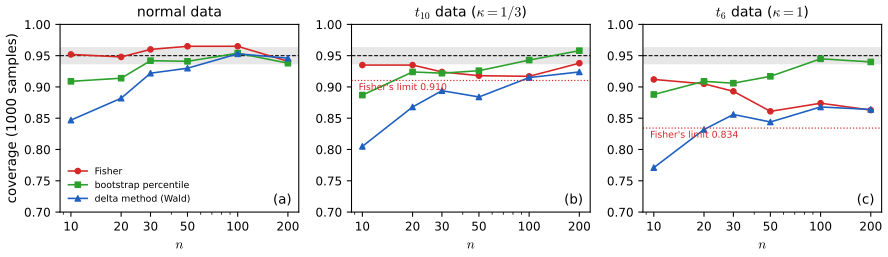
fig_14_s2, corr_demo. Supplementary figure; answers Wasserman (2004), Exercise 14.6, and extends it to non-normal data. Download: PDF · SVGFilling the gap 14.7: why the standard error is \(1/\sqrt{n-3}\) p. 234, "can be shown"
Assume normal data. (a) If \(\rho=0\), then \(\hrho^2\)\({}\sim\Bet\big(\tfrac12,\tfrac{n-2}2\big)\), \(\hrho\) is symmetric about 0, and \(\hrho\sqrt{n-2}/\sqrt{1-\hrho^2}\)\({}\sim t_{n-2}\). (b) Hence, at \(\rho=0\), \(z=\artanh\hrho\) satisfies
\[ \V(z)=\frac1{n-1}+\frac2{(n-1)(n+1)}+R_n,\qquad0\le R_n\le\frac{15}{(n-4)(n-1)(n+1)}\quad(n\gt4), \]while \(\frac1{n-3}\)\({}=\frac1{n-1}+\frac2{(n-1)(n-3)}\): the two agree up to \(O(n^{-3})\), and \(1/n\) does not (it is off by about \(3/n^2\)). The choice \(n-3\) is the one that makes the first two terms of the variance right. (c) For general \(\rho\), the exact density of \(\hrho\) is known (Fisher, 1915); in Hotelling's (1953) form,
\[ f_{\hrho}(r)=\frac{(n-2)\,\Gamma(n-1)}{\sqrt{2\pi}\,\Gamma(n-\frac12)}\,\frac{(1-\rho^2)^{(n-1)/2}(1-r^2)^{(n-4)/2}}{(1-\rho r)^{n-3/2}}\;{}_2F_1\Big(\tfrac12,\tfrac12;n-\tfrac12;\tfrac{1+\rho r}2\Big),\qquad-1\lt r\lt1, \]and its expansions give \(\E z\)\({}=\artanh\rho+\frac{\rho}{2(n-1)}+O(n^{-2})\) and \(\V(z)\)\({}=\frac1{n-1}+\frac{4-\rho^2}{2(n-1)^2}+O(n^{-3})\) (Fisher, 1921). So \(1/(n-3)\) is right to second order at \(\rho=0\) and slightly too large when \(|\rho|\) is large, which makes the interval a little conservative; the small bias \(\rho/\{2(n-1)\}\) works the other way.
Derivation of (a) and (b)
(a) The null distribution. When \(\rho=0\) the two coordinates of a bivariate normal are independent (Filling the gap 3.7(5)). Condition on the first coordinates \(\bx_1=(x_{11},\dots,x_{1n})\), assumed not all equal (this has probability one), and let \(\bu\)\({}=(\bx_1-\overline x_1\bone)/\|\bx_1-\overline x_1\bone\|\), a unit vector orthogonal to \(\bone\). Complete \(\bone/\sqrt n,\bu\) to an orthonormal basis \(\bone/\sqrt n,\bu,\bv_3,\dots,\bv_n\) of \(\R^n\). The vector \(\bX_2\)\({}=(X_{21},\dots,X_{2n})^\T\)\({}\sim\N(\mu_2\bone,\sigma_2^2\bI)\) is independent of \(\bx_1\); its coordinates in the new basis, \(Y_1=\bu^\T\bX_2\) and \(Y_j=\bv_j^\T\bX_2\) (\(j\ge3\)), are independent \(\N(0,\sigma_2^2)\) (an orthogonal transformation of a spherical normal vector is spherical, and \(\bu,\bv_j\perp\bone\) kill the mean). Then \(\sum_i(X_{2i}-\overline X_2)^2\)\({}=\|\bX_2\|^2-(\bone^\T\bX_2)^2/n\)\({}=Y_1^2+Q\) with \(Q=\sum_{j\ge3}Y_j^2\), and \(\sum_i(x_{1i}-\overline x_1)(X_{2i}-\overline X_2)\)\({}=\|\bx_1-\overline x_1\bone\|\,Y_1\). So
\[ \hrho=\frac{Y_1}{\sqrt{Y_1^2+Q}},\qquad\hrho^2=\frac{Y_1^2}{Y_1^2+Q},\qquad\frac{\hrho\sqrt{n-2}}{\sqrt{1-\hrho^2}}=\frac{Y_1}{\sqrt{Q/(n-2)}}, \]with \(Y_1^2/\sigma_2^2\sim\chi^2_1\) and \(Q/\sigma_2^2\sim\chi^2_{n-2}\) independent. The ratio \(A/(A+B)\) of independent \(\chi^2_a\) and \(\chi^2_b\) variables is \(\Bet(a/2,b/2)\) (the gamma-beta relation, Result 2.8), and \(Y_1/\sqrt{Q/(n-2)}\sim t_{n-2}\) by the definition of Student's \(t\) (Result 2.9). Symmetry: \(Y_1\mapsto-Y_1\) preserves the joint law. None of these conditional laws depends on \(\bx_1\), so they are also the unconditional laws.
(b) Moments. For \(B\sim\Bet(a,b)\), \(\E B^m\)\({}=\prod_{i=0}^{m-1}\frac{a+i}{a+b+i}\); with \(a=\tfrac12\), \(a+b=\tfrac{n-1}2\): \(\E\hrho^2=\frac1{n-1}\), \(\E\hrho^4=\frac{3}{(n-1)(n+1)}\), and \(\E\{B^3/(1-B)\}\)\({}=\frac{a(a+1)(a+2)}{(b-1)(a+b)(a+b+1)}\)\({}=\frac{15}{(n-4)(n-1)(n+1)}\) for \(b\gt1\), i.e. \(n\gt4\).
The series. From \(\artanh r=\sum_{i\ge0}r^{2i+1}/(2i+1)\) for \(|r|\lt1\), the coefficient of \(r^{2m}\) in \((\artanh r)^2\) is
\[ c_m=\sum_{i=0}^{m-1}\frac1{(2i+1)(2m-2i-1)}=\frac1{2m}\sum_{i=0}^{m-1}\Big(\frac1{2i+1}+\frac1{2m-2i-1}\Big)=\frac1m\sum_{j=1}^m\frac1{2j-1}, \]so \(c_1=1\), \(c_2=\tfrac23\), and \(0\lt c_m\le1\) (an average of \(m\) numbers in \((0,1]\)). Therefore \(0\)\({}\le z^2-\hrho^2-\tfrac23\hrho^4\)\({}=\sum_{m\ge3}c_m\hrho^{2m}\)\({}\le\sum_{m\ge3}\hrho^{2m}\)\({}=\hrho^6/(1-\hrho^2)\). By symmetry \(\E z=0\), so \(\V(z)\)\({}=\E z^2\)\({}=\E\hrho^2+\tfrac23\E\hrho^4+R_n\) with \(0\le R_n\le\E\{\hrho^6/(1-\hrho^2)\}\); inserting the moments gives the display. Finally \(\frac1{n-3}-\frac1{n-1}-\frac2{(n-1)(n+1)}\)\({}=\frac{8}{(n-1)(n-3)(n+1)}\)\({}=O(n^{-3})\), while \(\frac1n-\frac1{n-1}-\frac2{(n-1)(n+1)}\)\({}=-\frac{3n+1}{n(n-1)(n+1)}\) is of order \(n^{-2}\). ∎
(c) is quoted. The density integrates to one and its moments agree with simulation; integrating it after the substitution \(r=\tanh z\) gives the exact mean and variance of \(z\) used in Figure 14.S3(c), and confirms both expansions numerically. At \(n=10\), \(\sqrt{(n-3)\V(z)}\) is 0.997, 0.990, 0.978 and 0.969 for \(\rho=0,0.5,0.8,0.95\). Integrating it over Fisher's interval gives the exact coverage of the interval: 0.9504 at \(n=10\) and 0.9500 at \(n=100\) for \(\rho=1/\sqrt2\), against 0.840 and 0.939 for the delta-method interval.
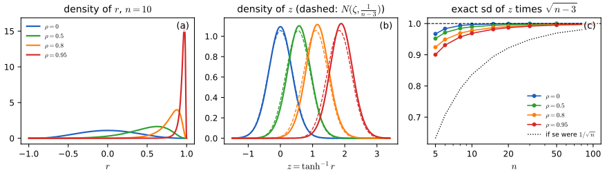
fig_14_s3, r_density, z_moments. Supplementary figure; illustrates Wasserman (2004), Section 14.2. Download: PDF · SVG14.3 Multivariate Normal
p. 234 \(\bX\sim\N(\bmu,\bSigma)\) if it has density
\[ f(\bx;\bmu,\bSigma)=\frac1{(2\pi)^{k/2}|\bSigma|^{1/2}}\exp\Big\{-\frac12(\bx-\bmu)^\T\bSigma^{-1}(\bx-\bmu)\Big\}, \tag{14.7} \]with \(\bmu\in\R^k\) and \(\bSigma\) symmetric positive definite; then \(\E(\bX)=\bmu\) and \(\V(\bX)=\bSigma\).
See also: Chapter 2, Result 2.15 and Result 2.16, and Chapter 3, Filling the gap 3.7, where all of the following is proved; Foundations of Deep Learning, Section 3.2; Bayesian and Probabilistic Machine Learning, Section 2.3.
Theorem 14.2 (properties of the multivariate normal) p. 235
- If \(\bZ\sim\N(\bzero,\bI)\) and \(\bX=\bmu+\bSigma^{1/2}\bZ\), then \(\bX\sim\N(\bmu,\bSigma)\).
- If \(\bX\sim\N(\bmu,\bSigma)\), then \(\bSigma^{-1/2}(\bX-\bmu)\)\({}\sim\N(\bzero,\bI)\).
- If \(\bX\sim\N(\bmu,\bSigma)\) and \(\ba\in\R^k\), then \(\ba^\T\bX\)\({}\sim\N(\ba^\T\bmu,\ba^\T\bSigma\ba)\).
- \(V\)\({}=(\bX-\bmu)^\T\bSigma^{-1}(\bX-\bmu)\)\({}\sim\chi^2_k\).
(The book writes \(\N(0,1)\) in parts 1 and 2; the standard normal vector \(\N(\bzero,\bI)\) is meant.)
Filling the gap 14.8: proof of Theorem 14.2, and normality as a property of linear combinations
Theorem 14.2 holds, and \(\bSigma^{1/2}\) in part 1 may be replaced by any \(\bB\) with \(\bB\bB^\T=\bSigma\). Moreover, \(\bX\) is \(\N(\bmu,\bSigma)\) if and only if \(\ba^\T\bX\)\({}\sim\N(\ba^\T\bmu,\ba^\T\bSigma\ba)\) for every \(\ba\); this characterisation is used as the definition of a normal vector when \(\bSigma\) is singular and (14.7) does not exist (the limit in Theorem 14.6 is such a vector).
Proof (sketch; the full proofs are in Chapters 2 and 3)
1. \(\bZ\) has density \((2\pi)^{-k/2}e^{-\bz^\T\bz/2}\); the map \(\bz\mapsto\bmu+\bB\bz\) is invertible with Jacobian determinant \(|\bB|=|\bSigma|^{1/2}\) (up to sign), and \(\bz^\T\bz\)\({}=(\bx-\bmu)^\T\bB^{-\T}\bB^{-1}(\bx-\bmu)\)\({}=(\bx-\bmu)^\T\bSigma^{-1}(\bx-\bmu)\); the change-of-variables formula gives (14.7). 2. The inverse map. 3. \(\ba^\T\bX=\ba^\T\bmu+(\bB^\T\ba)^\T\bZ\) is a constant plus a sum of independent normals, hence normal, with the variance of Theorem 14.1. 4. \(V=\bZ^\T\bZ=\sum Z_i^2\). Full details: Result 2.16, Filling the gap 3.7.
The characterisation. If every \(\ba^\T\bX\) is \(\N(\ba^\T\bmu,\ba^\T\bSigma\ba)\), its moment generating function at 1 is \(\E e^{\ba^\T\bX}\)\({}=\exp(\ba^\T\bmu+\tfrac12\ba^\T\bSigma\ba)\) for every \(\ba\): this is the joint moment generating function of \(\bX\), and it equals that of \(\N(\bmu,\bSigma)\) (Filling the gap 3.7(2)); the uniqueness theorem for moment generating functions identifies the law. The converse is part 3. ∎
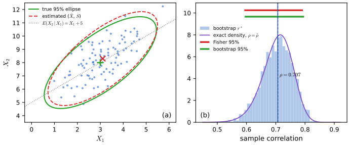
fig_14_s1, exercise5. Supplementary figure; answers Wasserman (2004), Exercise 14.5. Download: PDF · SVGConditional distributions are not in the book's Chapter 14 but are proved in Chapter 2 (Result 2.16, for conditioning on a sub-vector). The following form, conditioning on a linear combination, contains that one and explains two phenomena: regression to the mean, and the dependence created by conditioning on a total.
Filling the gap 14.9: conditioning a normal vector on a linear combination
Let \(\bX\sim\N(\bmu,\bSigma)\), \(\ba\ne\bzero\), \(W=\ba^\T\bX\) and \(\bbeta=\bSigma\ba/(\ba^\T\bSigma\ba)\). Then \(\bm{R}=\bX-\bbeta W\) is independent of \(W\), and given \(W=c\),
\[ \bX\given\{\ba^\T\bX=c\}\ \sim\ \N\Big(\bmu+\bSigma\ba\,\frac{c-\ba^\T\bmu}{\ba^\T\bSigma\ba},\ \bSigma-\frac{\bSigma\ba\ba^\T\bSigma}{\ba^\T\bSigma\ba}\Big), \]a singular normal law carried by the line (hyperplane) \(\ba^\T\bx=c\). With \(\ba=\be_1\) and \(k=2\): \(X_2\given X_1\)\({}=x\)\({}\sim\N\big(\mu_2+\rho\frac{\sigma_2}{\sigma_1}(x-\mu_1),\ \sigma_2^2(1-\rho^2)\big)\).
Derivation
\((\bm{R},W)\) is a linear function of \(\bX\), hence jointly normal (Filling the gap 14.8), and \(\Cov(\bm{R},W)\)\({}=\Cov(\bX,W)-\bbeta\V(W)\)\({}=\bSigma\ba-\bbeta\,\ba^\T\bSigma\ba\)\({}=\bzero\). Jointly normal and uncorrelated means independent (Filling the gap 3.7(5)). So \(\bX=\bm{R}+\bbeta W\) with \(\bm{R}\) independent of \(W\): conditionally on \(W=c\), \(\bX\) has the law of \(\bm{R}+\bbeta c\). (This is a rigorous version of conditioning on the null event \(\{W=c\}\): it defines a regular conditional distribution, the one obtained as the limit of conditioning on \(|W-c|\le h\) as \(h\downarrow0\), see below.) Finally \(\E\bm{R}=\bmu-\bbeta\ba^\T\bmu\) and
\[ \V(\bm{R})=\bSigma-\bbeta\ba^\T\bSigma-\bSigma\ba\bbeta^\T+\bbeta\bbeta^\T\,\ba^\T\bSigma\ba=\bSigma-\frac{\bSigma\ba\ba^\T\bSigma}{\ba^\T\bSigma\ba}. \]The case \(\ba=\be_1\), \(k=2\): \(\bbeta=(1,\sigma_{12}/\sigma_1^2)^\T\) and \(\sigma_{12}=\rho\sigma_1\sigma_2\). ∎
Three consequences. (i) Exercise 5's distribution: \(\bmu=(3,8)^\T\), \(\sigma_1^2=1\), \(\sigma_{12}=1\), \(\sigma_2^2=2\) give \(X_2\given X_1=x\sim\N(x+5,1)\), the dotted line of Figure 14.S1(a). (ii) Regression to the mean: for standardised variables, \(\E(X_2\given X_1=x)=\rho x\): a unit two standard deviations above average on \(X_1\) is expected only \(2\rho\) above average on \(X_2\), and symmetrically \(\E(X_1\given X_2=y)=\rho y\). The two regression lines differ, and neither is the major axis of the ellipse. (iii) Conditioning on a total: if \(X_1,X_2\iid\N(m,\sigma^2)\), then given \(X_1+X_2=c\), \(X_1\sim\N(c/2,\sigma^2/2)\) and \(X_2=c-X_1\): independent variables become perfectly negatively dependent. This is the normal counterpart of the negative covariances of the multinomial (Theorem 14.4), which is the law of independent Poisson counts given their total.
Conditioning by simulation. Keeping only the simulated points with \(|W-c|\le h\) gives \(\bX\) given \(|W-c|\le h\): for the coordinate \(Y=\bb^\T\bX\), its law has mean \(\E(Y\given W=c)\) shifted by \(\beta_Y\{\E(W\given|W-c|\le h)-c\}\) and variance \(\V(Y\given W)+\beta_Y^2\,\V(W\given|W-c|\)\({}\le h)\), with \(\beta_Y\)\({}=\bb^\T\bSigma\ba/(\ba^\T\bSigma\ba)\) (decompose \(Y=\bb^\T\bm{R}+\beta_YW\)). Since \(\V(W\given|W-c|\le h)\approx h^2/3\) for small \(h\), the strip estimate converges to the conditional law as \(h\to0\), and a wide strip inflates the variance.
Theorem 14.3 (the normal log-likelihood and the MLE), as corrected p. 235, (14.8)
For a sample \(\bX_1,\dots,\bX_n\) from \(\N(\bmu,\bSigma)\), up to the constant \(-\frac{nk}2\log(2\pi)\),
\[ \ell(\bmu,\bSigma)=-\frac n2(\Xbar-\bmu)^\T\bSigma^{-1}(\Xbar-\bmu)-\frac{n-1}2\tr(\bSigma^{-1}\bS)-\frac n2\log|\bSigma| \](equivalently \(-\frac n2\tr(\bSigma^{-1}\hSigma)\) in the middle). The book prints \(-\frac n2\tr(\bSigma^{-1}\bS)\), which would be right only if \(\bS\) had divisor \(n\). If \(n\ge k+1\), the MLE exists, is unique, and is
\[ \widehat\bmu=\Xbar\qquad\text{and}\qquad\hSigma=\Big(\frac{n-1}n\Big)\bS. \tag{14.8} \]If \(n\le k\), the likelihood is unbounded and there is no MLE.
The log-likelihood is derived in the Appendix; the book stops there and does not show that (14.8) maximises it. Note that \((\Xbar,\bS)\) is sufficient (the likelihood depends on the data only through them, the factorisation theorem).
Filling the gap 14.10: (14.8) is the unique global maximum, and when it does not exist p. 235
Assume \(n\ge k+1\). Then \(\hSigma\) is positive definite with probability one, and for every \(\bmu\) and every positive definite \(\bSigma\),
\[ \ell(\bmu,\bSigma)\le\ell(\Xbar,\hSigma)=-\frac{nk}2\{1+\log(2\pi)\}-\frac n2\log|\hSigma|, \]with equality only at \((\Xbar,\hSigma)\). If \(n\le k\), \(\sup\ell=+\infty\).
Derivation (no matrix calculus)
\(\hSigma\) is positive definite. By Filling the gap 14.11, \(n\hSigma=\sum_{j=2}^n\bY_j\bY_j^\T\) with \(\bY_2,\dots,\bY_n\iid\N(\bzero,\bSigma)\). If \(\bY_2,\dots,\bY_{k+1}\) are linearly independent, \(\bx^\T n\hSigma\bx\)\({}=\sum_j(\bY_j^\T\bx)^2\)\({}\gt0\) for every \(\bx\ne\bzero\). They are, with probability one: given \(\bY_2,\dots,\bY_{j-1}\), the next \(\bY_j\) has a density on \(\R^k\) and falls in their span, a subspace of dimension less than \(k\) and hence of Lebesgue measure zero, with probability zero.
Step 1, the mean. \(\bSigma^{-1}\) is positive definite, so the first term of \(\ell\) is \(\le0\), with equality iff \(\bmu=\Xbar\). Hence \(\ell(\bmu,\bSigma)\)\({}\le\ell(\Xbar,\bSigma)\)\({}=\text{const}+\frac n2h(\bSigma)\) with \(h(\bSigma)\)\({}=-\log|\bSigma|-\tr(\bSigma^{-1}\hSigma)\).
Step 2, the covariance. Let \(\bM\)\({}=\hSigma^{1/2}\bSigma^{-1}\hSigma^{1/2}\), symmetric positive definite with eigenvalues \(\lambda_1,\dots,\lambda_k\gt0\). By the trace identity, \(\tr(\bSigma^{-1}\hSigma)\)\({}=\tr(\hSigma^{1/2}\bSigma^{-1}\hSigma^{1/2})\)\({}=\tr\bM\)\({}=\sum_i\lambda_i\), and \(|\bM|\)\({}=|\hSigma|/|\bSigma|\)\({}=\prod_i\lambda_i\). So
\[ h(\bSigma)=-\log|\hSigma|+\sum_{i=1}^k(\log\lambda_i-\lambda_i)\le-\log|\hSigma|-k, \]because \(\log\lambda-\lambda\le-1\) for \(\lambda\gt0\), with equality only at \(\lambda=1\) (the function is concave with derivative \(1/\lambda-1\), zero at 1). Equality throughout forces every \(\lambda_i=1\), i.e. \(\bM=\bI\), i.e. \(\bSigma=\hSigma\). Substituting \(\bSigma=\hSigma\) gives the maximum value.
No MLE when \(n\le k\). Then \(\hSigma\) (a sum of \(n-1\lt k\) outer products) is singular: some unit \(\bu\) has \(\hSigma\bu=\bzero\). Take \(\bSigma_\epsilon=\hSigma+\epsilon\bI\). Then \(\tr(\bSigma_\epsilon^{-1}\hSigma)\le k\), while \(|\bSigma_\epsilon|\)\({}\le\epsilon\,(\lambda_{\max}+\epsilon)^{k-1}\)\({}\to0\), so \(\ell(\Xbar,\bSigma_\epsilon)\)\({}\ge\text{const}-\frac n2\log|\bSigma_\epsilon|-\frac{nk}2\)\({}\to+\infty\). The likelihood can be made arbitrarily large by squeezing the fitted normal onto the hyperplane that contains the data. ∎
Foundations of Deep Learning proves the same result by differentiating and checking concavity (Filling the gap 3.4); the eigenvalue argument above avoids derivatives with respect to a symmetric matrix. The same argument with \(\bmu\) fixed shows that \(\max_{\bSigma}\ell(\bmu,\bSigma)\) is attained at \(\hSigma_{\bmu}\)\({}=n^{-1}\sum_i(\bX_i-\bmu)(\bX_i-\bmu)^\T\), which is used for the likelihood ratio test in Filling the gap 14.13.
Filling the gap 14.11: the joint distribution of \(\Xbar\) and \(\bS\), and the Wishart distribution
For \(\bX_1,\dots,\bX_n\iid\N(\bmu,\bSigma)\): \(\Xbar\sim\N(\bmu,\bSigma/n)\); \((n-1)\bS=\sum_{j=2}^n\bY_j\bY_j^\T\) with \(\bY_2,\dots,\bY_n\iid\N(\bzero,\bSigma)\); and \(\Xbar\) and \(\bS\) are independent. A matrix \(\bW=\sum_{j=1}^m\bY_j\bY_j^\T\) with \(\bY_j\iid\N(\bzero,\bSigma)\) has, by definition, the Wishart distribution \(\Wish_k(m,\bSigma)\); so \((n-1)\bS\sim\Wish_k(n-1,\bSigma)\). Its moments are \(\E\bW=m\bSigma\) and \(\V(W_{ab})\)\({}=m(\sigma_{ab}^2+\sigma_{aa}\sigma_{bb})\); for \(k=1\), \(\Wish_1(m,\sigma^2)=\sigma^2\chi^2_m\).
Derivation
A rotation of the sample. Let \(\bH\) be an \(n\times n\) orthogonal matrix whose first row is \(\bone^\T/\sqrt n\) (for instance the Helmert matrix, whose row \(j\ge2\) is \((1,\dots,1,-(j-1),0,\dots,0)/\sqrt{j(j-1)}\)). Put \(\bY_j=\sum_ih_{ji}\bX_i\), the rows of \(\bH\) times the \(n\times k\) data matrix. The \(\bY_j\) are jointly normal (linear in the independent normal \(\bX_i\)), with \(\E\bY_j=(\sum_ih_{ji})\bmu=\sqrt n\,\bmu\) if \(j=1\) and \(\bzero\) otherwise (rows \(j\ge2\) are orthogonal to the first, so their entries sum to zero), and
\[ \Cov(\bY_j,\bY_l)=\sum_{i}h_{ji}h_{li}\,\bSigma=(\bH\bH^\T)_{jl}\bSigma=\delta_{jl}\bSigma . \]Jointly normal with zero cross-covariances, the \(\bY_j\) are independent. Now \(\bY_1=\sqrt n\,\Xbar\), and orthogonality gives \(\sum_j\bY_j\bY_j^\T=\sum_i\bX_i\bX_i^\T\), so \(\sum_{j\ge2}\bY_j\bY_j^\T\)\({}=\sum_i\bX_i\bX_i^\T-n\Xbar\Xbar^\T\)\({}=(n-1)\bS\) (the identity of Filling the gap 14.3 with \(\bmu=\bzero\)). Thus \(\Xbar\)\({}=\bY_1/\sqrt n\)\({}\sim\N(\bmu,\bSigma/n)\) is a function of \(\bY_1\) and \(\bS\) a function of \(\bY_2,\dots,\bY_n\): they are independent, and \((n-1)\bS\sim\Wish_k(n-1,\bSigma)\).
Moments. \(\E\bY\bY^\T=\bSigma\), so \(\E\bW=m\bSigma\). For one \(\bY\sim\N(\bzero,\bSigma)\), Isserlis' identity (the fourth-moment computation of Filling the gap 14.5, unstandardised) gives \(\E(Y_a^2Y_b^2)\)\({}=\sigma_{aa}\sigma_{bb}+2\sigma_{ab}^2\), so \(\V(Y_aY_b)\)\({}=\sigma_{aa}\sigma_{bb}+\sigma_{ab}^2\), and independence over \(j\) multiplies by \(m\). Consequently \(\V(s_{ab})\)\({}=(\sigma_{ab}^2+\sigma_{aa}\sigma_{bb})/(n-1)\). For \(k=1\), \(W\)\({}=\sum_jY_j^2\)\({}=\sigma^2\sum_j(Y_j/\sigma)^2\)\({}\sim\sigma^2\chi^2_m\), which recovers \((n-1)s^2/\sigma^2\sim\chi^2_{n-1}\) independent of \(\overline X\). ∎
For \(m\ge k\), \(\bW\) is positive definite with probability one (as in Filling the gap 14.10) and has density proportional to \(|\bW|^{(m-k-1)/2}\exp\{-\tfrac12\tr(\bSigma^{-1}\bW)\}\) on positive definite matrices (Wishart, 1928); it is derived, with its role as a conjugate prior, in the companion course's toolkit, Section 5.4. We will not need the density.
Hotelling's \(T^2\) test (an addition)
The book has no test for a mean vector. The multivariate version of the one-sample t-test is the natural next step after (14.8), and it is the cleanest application of Filling the gap 14.11.
Result 14.7 (Hotelling's \(T^2\); addition)
Let \(\bX_1,\dots,\bX_n\iid\N(\bmu,\bSigma)\) with \(n\gt k\), and \(\bmu_0\) fixed. Define
\[ T^2=n(\Xbar-\bmu_0)^\T\bS^{-1}(\Xbar-\bmu_0). \]Then \(\dfrac{n-k}{k(n-1)}T^2\) has the \(F_{k,n-k}\) distribution when \(\bmu=\bmu_0\), and the noncentral \(F_{k,n-k}\) distribution with noncentrality \(\lambda\)\({}=n(\bmu-\bmu_0)^\T\bSigma^{-1}(\bmu-\bmu_0)\) otherwise. The level-\(\alpha\) test rejects \(H_0:\bmu=\bmu_0\) when \(T^2\gt\frac{k(n-1)}{n-k}F_{k,n-k,\alpha}\). For \(k=1\), \(T^2\) is the square of the one-sample t-statistic.
Filling the gap 14.12: proof of Result 14.7
The key lemma: if \(\bW\sim\Wish_k(m,\bSigma)\) with \(m\ge k\) and \(\bv\ne\bzero\) is fixed, then \(\dfrac{\bv^\T\bSigma^{-1}\bv}{\bv^\T\bW^{-1}\bv}\)\({}\sim\chi^2_{m-k+1}\).
Proof
The lemma. (i) Reduce to \(\bSigma=\bI\). \(\bW=\bSigma^{1/2}\bW_0\bSigma^{1/2}\) with \(\bW_0=\sum_j\bZ_j\bZ_j^\T\), \(\bZ_j\)\({}=\bSigma^{-1/2}\bY_j\iid\N(\bzero,\bI)\), so \(\bW_0\sim\Wish_k(m,\bI)\). With \(\bu=\bSigma^{-1/2}\bv\), \(\bv^\T\bW^{-1}\bv=\bu^\T\bW_0^{-1}\bu\) and \(\bv^\T\bSigma^{-1}\bv=\bu^\T\bu\). The ratio is unchanged by scaling \(\bu\), so take \(\|\bu\|=1\). (ii) Rotate. For an orthogonal \(\bG\) with \(\bG\bu=\be_1\), \(\bG\bW_0\bG^\T\)\({}=\sum_j(\bG\bZ_j)(\bG\bZ_j)^\T\) is again \(\Wish_k(m,\bI)\) (the \(\bG\bZ_j\) are again iid \(\N(\bzero,\bI)\)), and \(\bu^\T\bW_0^{-1}\bu\)\({}=\be_1^\T(\bG\bW_0\bG^\T)^{-1}\be_1\). So the ratio has the law of \(1/(\bW_0^{-1})_{11}\). (iii) Schur complement. Partition \(\bW_0\) with blocks \(w_{11}\), \(\bm{w}_{12}\), \(\bW_{22}\) (sizes \(1\) and \(k-1\)). The partitioned inverse (Result 3.8 of the companion course) gives \(1/(\bW_0^{-1})_{11}\)\({}=w_{11}-\bm{w}_{12}\bW_{22}^{-1}\bm{w}_{21}\). (iv) A regression residual. Stack the \(\bZ_j^\T\) into an \(m\times k\) matrix with iid \(\N(0,1)\) entries, first column \(\bm{y}\), remaining columns \(\bm{Z}_2\). Then \(\bW_0\)\({}=[\bm{y},\bm{Z}_2]^\T[\bm{y},\bm{Z}_2]\) and \(w_{11}-\bm{w}_{12}\bW_{22}^{-1}\bm{w}_{21}\)\({}=\bm{y}^\T(\bI-\bP_2)\bm{y}\), with \(\bP_2\)\({}=\bm{Z}_2(\bm{Z}_2^\T\bm{Z}_2)^{-1}\bm{Z}_2^\T\) the orthogonal projection onto the column space of \(\bm{Z}_2\), which has dimension \(k-1\) with probability one. Given \(\bm{Z}_2\), \(\bm{y}\sim\N(\bzero,\bI_m)\) is independent of it and \(\bI-\bP_2\) is a fixed projection of rank \(m-k+1\); writing \(\bm{y}\) in an orthonormal basis adapted to it, \(\bm{y}^\T(\bI-\bP_2)\bm{y}\) is a sum of \(m-k+1\) squared independent standard normals, \(\chi^2_{m-k+1}\). This conditional law does not depend on \(\bm{Z}_2\), so it is the unconditional law.
The theorem. By Filling the gap 14.11, \(\bd\)\({}=\sqrt n(\Xbar-\bmu_0)\)\({}\sim\N(\sqrt n(\bmu-\bmu_0),\bSigma)\) is independent of \(\bW=(n-1)\bS\sim\Wish_k(n-1,\bSigma)\), and \(T^2=(n-1)\bd^\T\bW^{-1}\bd\). Write
\[ \frac{T^2}{n-1}=\frac{Q_1}{Q_2},\qquad Q_1=\bd^\T\bSigma^{-1}\bd,\qquad Q_2=\frac{\bd^\T\bSigma^{-1}\bd}{\bd^\T\bW^{-1}\bd}. \]Conditionally on \(\bd\), \(\bW\) keeps its law (independence), so by the lemma with \(m=n-1\), \(Q_2\given\bd\sim\chi^2_{n-k}\) whatever \(\bd\) is; hence \(Q_2\sim\chi^2_{n-k}\) and \(Q_2\) is independent of \(\bd\), so of \(Q_1\). Under \(H_0\), \(Q_1\sim\chi^2_k\) (Theorem 14.2(4)); in general \(\bSigma^{-1/2}\bd\)\({}\sim\N(\sqrt n\bSigma^{-1/2}(\bmu-\bmu_0),\bI)\), so \(Q_1\) is noncentral \(\chi^2_k\) with noncentrality \(\lambda\). Therefore \(\frac{n-k}{k(n-1)}T^2\)\({}=\frac{Q_1/k}{Q_2/(n-k)}\) is a ratio of independent chi-squares over their degrees of freedom: \(F_{k,n-k}\), central under \(H_0\). For \(k=1\), \(T^2=n(\overline X-\mu_0)^2/s^2=t^2\). ∎
Filling the gap 14.13: \(T^2\) is the likelihood ratio test and the largest squared t-statistic, and how it compares with separate t-tests
(a) Union–intersection. For \(\ba\ne\bzero\) let \(t_{\ba}\)\({}=\sqrt n\,\ba^\T(\Xbar-\bmu_0)/\sqrt{\ba^\T\bS\ba}\), the one-sample t-statistic of the univariate data \(\ba^\T\bX_i\). Then \(T^2=\max_{\ba\ne\bzero}t_{\ba}^2\), attained at \(\ba\propto\bS^{-1}(\Xbar-\bmu_0)\). Consequently the intervals \(\ba^\T\bmu\in\ba^\T\Xbar\pm\sqrt{c_\alpha\,\ba^\T\bS\ba/n}\), \(c_\alpha\)\({}=\frac{k(n-1)}{n-k}F_{k,n-k,\alpha}\), hold simultaneously for all \(\ba\) with probability \(1-\alpha\).
(b) Likelihood ratio. The likelihood ratio statistic for \(H_0:\bmu=\bmu_0\) (with \(\bSigma\) unknown) is \(\Lambda=\big(1+T^2/(n-1)\big)^{-n/2}\), a decreasing function of \(T^2\): the likelihood ratio test is the \(T^2\) test.
(c) Against separate t-tests. Testing each coordinate at level \(\alpha\) has size larger than \(\alpha\) (up to \(1-(1-\alpha)^k\) for independent coordinates); the Bonferroni version (level \(\alpha/k\) each) has size at most \(\alpha\). The Bonferroni acceptance region is a rectangle in the \((t_1,\dots,t_k)\) coordinates and ignores the correlations; the \(T^2\) region is an ellipsoid that uses them. Which is more powerful depends on the direction of \(\bmu-\bmu_0\): \(T^2\) depends on it only through the Mahalanobis length \(\lambda\), which is large for shifts "against" the correlation and small for shifts "along" it.
Derivation
(a) With \(\bd=\Xbar-\bmu_0\), Cauchy–Schwarz for the vectors \(\bS^{1/2}\ba\) and \(\bS^{-1/2}\bd\) gives \((\ba^\T\bd)^2\)\({}=\{(\bS^{1/2}\ba)^\T(\bS^{-1/2}\bd)\}^2\)\({}\le(\ba^\T\bS\ba)(\bd^\T\bS^{-1}\bd)\), with equality iff \(\bS^{1/2}\ba\propto\bS^{-1/2}\bd\), i.e. \(\ba\propto\bS^{-1}\bd\). Multiply by \(n/(\ba^\T\bS\ba)\). Since \(T^2\le c_\alpha\) (with probability \(1-\alpha\) at the true \(\bmu\)) is equivalent to \(t_{\ba}^2\le c_\alpha\) for all \(\ba\), the simultaneous intervals follow. In particular \(T^2\ge\max_jt_j^2\) for the coordinate statistics.
(b) By Filling the gap 14.10, \(\max_{\bmu,\bSigma}L=C|\hSigma|^{-n/2}\) and \(\max_{\bSigma}L(\bmu_0,\bSigma)\)\({}=C|\hSigma_{\bmu_0}|^{-n/2}\) with the same constant \(C=(2\pi)^{-nk/2}e^{-nk/2}\) and \(\hSigma_{\bmu_0}\)\({}=n^{-1}\sum_i(\bX_i-\bmu_0)(\bX_i-\bmu_0)^\T\)\({}=\hSigma+\bd\bd^\T\) (Filling the gap 14.3). The determinant lemma, \(|\bA+\bb\bb^\T|\)\({}=|\bA|(1+\bb^\T\bA^{-1}\bb)\) (because \(\bI+\bA^{-1}\bb\bb^\T\) has eigenvalue \(1+\bb^\T\bA^{-1}\bb\) on \(\bA^{-1}\bb\) and 1 on the hyperplane orthogonal to \(\bb\); see the toolkit), gives
\[ \Lambda^{2/n}=\frac{|\hSigma|}{|\hSigma+\bd\bd^\T|}=\frac1{1+\bd^\T\hSigma^{-1}\bd}=\frac1{1+T^2/(n-1)}, \]since \(\hSigma^{-1}=\frac n{n-1}\bS^{-1}\).
(c) Under \(H_0\) each coordinate test rejects with probability \(\alpha\) (or \(\alpha/k\)); the union bound gives size at most \(k\cdot\alpha/k=\alpha\) for Bonferroni, and for independent coordinates the unadjusted size is exactly \(1-(1-\alpha)^k\) (0.0975 for \(k=2\)). For the power, take \(k=2\), unit variances and correlation \(\rho\), and \(\bmu-\bmu_0=c\,\bu\) with \(\|\bu\|=1\): \(\lambda=nc^2\,\bu^\T\bSigma^{-1}\bu\), which is \(nc^2/(1-\rho)\) for \(\bu\propto(1,-1)\) and \(nc^2/(1+\rho)\) for \(\bu\propto(1,1)\), a ratio of \((1+\rho)/(1-\rho)\), 9 when \(\rho=0.8\). The coordinate t-statistics see \(\sqrt n\,c/\sqrt2\) in both cases. So \(T^2\) is far more powerful against \((1,-1)\) and somewhat less powerful along \((1,1)\) (Figure 14.S4). ∎
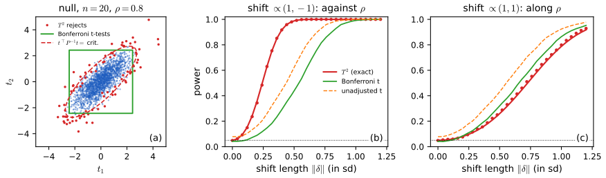
fig_14_s4, hotelling_demo. Supplementary figure; illustrates Result 14.7 and Filling the gap 14.13 (additions to Wasserman 2004, Section 14.3). Download: PDF · SVGFilling the gap 14.14: \(\bS\) is unbiased, but its eigenvalues are not
For any \(n\ge2\), \(\E\lambda_{\max}(\bS)\)\({}\ge\lambda_{\max}(\bSigma)\) and \(\E\lambda_{\min}(\bS)\)\({}\le\lambda_{\min}(\bSigma)\), while the average eigenvalue \(\tr(\bS)/k\) is unbiased: the sample eigenvalues are spread out around the true ones. When \(\bSigma=\bI\) and \(k/n\to\gamma\in(0,1)\), the sample eigenvalues fill the interval \([(1-\sqrt\gamma)^2,(1+\sqrt\gamma)^2]\) (Marchenko and Pastur, 1967, quoted).
Derivation
\(\lambda_{\max}(\bA)\)\({}=\max_{\|\bu\|=1}\bu^\T\bA\bu\) is a maximum of linear functions of the symmetric matrix \(\bA\), hence convex in \(\bA\). Jensen's inequality (Theorem 4.9, applied entrywise to the random matrix \(\bS\), or along the segment between any two values) gives \(\E\lambda_{\max}(\bS)\)\({}\ge\lambda_{\max}(\E\bS)\)\({}=\lambda_{\max}(\bSigma)\). Likewise \(\lambda_{\min}(\bA)\)\({}=\min_{\|\bu\|=1}\bu^\T\bA\bu\) is concave, so \(\E\lambda_{\min}(\bS)\)\({}\le\lambda_{\min}(\bSigma)\). The sum of the eigenvalues is \(\tr\bS\), and \(\E\tr\bS=\tr\bSigma\). ∎
The inequality is far from an equality when \(k/n\) is not small (Figure 14.S6(b): with \(k=10\), \(n=20\) and \(\bSigma=\bI\) the largest sample eigenvalue averages 2.5). This is why \(\bS\) is a poor estimate of the eigenvalues, and \(\bS^{-1}\) a poor estimate of the precision matrix, in high dimensions. A related exact fact: \(\E\bW^{-1}=\bSigma^{-1}/(m-k-1)\) for \(\bW\sim\Wish_k(m,\bSigma)\), \(m\gt k+1\) (Anderson, 2003), so \(\E\bS^{-1}=\frac{n-1}{n-k-2}\bSigma^{-1}\), inflated by a factor that grows as \(k\) approaches \(n\). PCA in the companion course meets the same instability (Filling the gap 7.18).
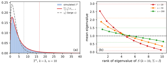
fig_14_s6. Supplementary figure; illustrates Filling the gaps 14.12 and 14.14 (additions to Wasserman 2004, Section 14.3). Download: PDF · SVG14.4 Multinomial
p. 235 Draw \(n\) balls with replacement from an urn with balls of \(k\) colours, colour \(j\) having probability \(p_j\) (\(p_j\ge0\), \(\sum_jp_j=1\)), and let \(X_j\) be the number of balls of the \(j\)-th colour. Then \(\bX=(X_1,\dots,X_k)\sim\Mult(n,\bp)\).
See also: Result 2.14 (the mass function) and Filling the gap 3.6 (the covariance) in this course; Bayesian and Probabilistic Machine Learning, Result 2.5; Foundations of Deep Learning, Result 3.3.
Theorem 14.4 (moments of the multinomial) p. 235
If \(\bX\sim\Mult(n,\bp)\), then \(X_j\sim\Bin(n,p_j)\), \(\E(\bX)=n\bp\) and \(\V(\bX)=n\bSigma\) with \(\bSigma=\diag(\bp)-\bp\bp^\T\): diagonal entries \(p_j(1-p_j)\), off-diagonal entries \(-p_ip_j\).
The book's proof computes \(\Cov(X_i,X_j)\) from the variance of \(X_i+X_j\sim\Bin(n,p_i+p_j)\), and says that the binomial margins "follow easily". The representation below gives both at once.
Filling the gap 14.15: the multinomial as a sum of indicator vectors p. 236
Let \(\bxi_i\in\{\be_1,\dots,\be_k\}\) record the colour of ball \(i\): \(\bxi_1,\dots,\bxi_n\) are iid with \(\P(\bxi_i=\be_j)=p_j\), and \(\bX=\sum_{i=1}^n\bxi_i\). Then \(\E\bxi_i=\bp\), \(\V(\bxi_i)=\bSigma\), which gives Theorem 14.4, and \(\bSigma\bone=\bzero\), so \(\rank\bSigma=k-1\) when all \(p_j\gt0\).
Derivation
Margins. \(X_j\)\({}=\sum_i\ind\{\text{ball }i\text{ has colour }j\}\) is a sum of \(n\) independent Bernoulli(\(p_j\)) variables, hence \(\Bin(n,p_j)\). The same argument with the event "colour \(i\) or \(j\)" gives \(X_i+X_j\sim\Bin(n,p_i+p_j)\), the fact the book's proof uses.
Moments. \(\E\bxi_i=\sum_jp_j\be_j=\bp\). Since exactly one coordinate of \(\bxi_i\) is 1, \(\bxi_i\bxi_i^\T=\diag(\bxi_i)\), so \(\E\bxi_i\bxi_i^\T=\diag(\bp)\) and \(\V(\bxi_i)=\diag(\bp)-\bp\bp^\T=\bSigma\). By independence and Filling the gap 14.3, \(\E\bX=n\bp\) and \(\V(\bX)=n\bSigma\).
Rank. \(\bSigma\bone=\bp-\bp(\bp^\T\bone)=\bzero\), as Filling the gap 14.2 predicts from \(\bone^\T\bX=n\). For \(\bx\perp\bone\), \(\bx^\T\bSigma\bx\)\({}=\sum_jp_jx_j^2-(\sum_jp_jx_j)^2\) is the variance of a random variable taking the value \(x_j\) with probability \(p_j\), which is zero only if all \(x_j\) are equal, i.e. (with \(\bx\perp\bone\)) \(\bx=\bzero\). So the null space is spanned by \(\bone\). ∎
Theorem 14.5 (the MLE) p. 236
The maximum likelihood estimator of \(\bp\) is \(\hp=\bX/n\), i.e. \(\widehat p_j=X_j/n\).
Filling the gap 14.16: the Lagrange point is the global maximum, also when some counts are zero p. 236
For every \(\bq\) in the simplex, \(\ell(\hp)-\ell(\bq)=n\,\KL(\hp,\bq)\ge0\), with equality iff \(\bq=\hp\). Here \(\ell(\bq)=\sum_jX_j\log q_j\) (with \(0\log0=0\)) and \(\KL(\hp,\bq)\)\({}=\sum_{j:\widehat p_j\gt0}\widehat p_j\log(\widehat p_j/q_j)\).
Derivation
The book sets the derivative of the Lagrangian to zero. That locates a stationary point only, and it divides by \(p_j\), which fails at the boundary of the simplex; if some \(X_j=0\), the maximiser has \(\widehat p_j=0\), on the boundary. The direct argument: if \(q_j=0\) for some \(j\) with \(X_j\gt0\), then \(\ell(\bq)=-\infty\lt\ell(\hp)\). Otherwise, terms with \(X_j=0\) vanish on both sides, and
\[ \ell(\hp)-\ell(\bq)=\sum_{j:X_j\gt0}X_j\log\frac{X_j/n}{q_j}=n\sum_{j:\widehat p_j\gt0}\widehat p_j\log\frac{\widehat p_j}{q_j}=n\,\KL(\hp,\bq)\ge0 \]by Gibbs' inequality (Result 4.10), with equality iff \(q_j=\widehat p_j\) for all \(j\) (if \(\sum_{j:\widehat p_j\gt0}q_j\lt1\), the divergence is strictly positive). ∎
So maximum likelihood here is minimum Kullback–Leibler divergence from the empirical distribution, the general principle of Chapter 9.
pp. 236–237 Directly, \(\V(\hp)=n^{-2}\V(\bX)=\bSigma/n\). The book remarks that the Fisher information gives the same answer; the multinomial's Fisher information is its Exercise 2, worked out next.
Filling the gap 14.17: the Fisher information of the multinomial (Exercise 2), and why it needs \(k-1\) parameters p. 236
Parametrise by \(\btheta=(p_1,\dots,p_{k-1})\), with \(p_k=1-\sum_{j\lt k}p_j\), and assume all \(p_j\gt0\). The Fisher information of \(n\) observations (one \(\Mult(n,\bp)\) count vector) is
\[ I_n(\btheta)=n\Big(\diag\big(\tfrac1{p_1},\dots,\tfrac1{p_{k-1}}\big)+\frac1{p_k}\bone\bone^\T\Big),\qquad I_n(\btheta)^{-1}=\frac1n\big(\diag(\btheta)-\btheta\btheta^\T\big), \]which is exactly \(\V(\widehat p_1,\dots,\widehat p_{k-1})\): the MLE attains the Cramér–Rao bound for every \(n\). The \(k\times k\) matrix \(\bSigma/n\) is recovered as \(\bm{J}I_n^{-1}\bm{J}^\T\) with \(\bm{J}=\binom{\bI_{k-1}}{-\bone^\T}\), the Jacobian of \(\btheta\mapsto\bp\); it is singular, and no \(k\)-parameter information matrix exists because the \(p_j\) cannot vary freely.
Derivation
\(\ell(\btheta)\)\({}=\sum_{j\lt k}X_j\log\theta_j+X_k\log(1-\bone^\T\btheta)\) plus a constant. Score: \(\partial\ell/\partial\theta_j\)\({}=X_j/\theta_j-X_k/p_k\). Its mean is \(np_j/p_j-np_k/p_k=0\), as it must be. Second derivatives: \(\partial^2\ell/\partial\theta_j\partial\theta_l\)\({}=-\delta_{jl}X_j/\theta_j^2-X_k/p_k^2\). Taking \(-\E\) with \(\E X_j=np_j\) gives \(I_n\). (The same matrix is the covariance of the score, by the information identity, Theorem 9.17.)
Inverse. With \(\bD=\diag(1/\theta_j)\) and the Sherman–Morrison formula \((\bD+\bb\bb^\T)^{-1}\)\({}=\bD^{-1}-\bD^{-1}\bb\bb^\T\bD^{-1}/(1+\bb^\T\bD^{-1}\bb)\), \(\bb=\bone/\sqrt{p_k}\):
\[ \Big(\bD+\frac{\bone\bone^\T}{p_k}\Big)^{-1}=\diag(\btheta)-\frac{\btheta\btheta^\T/p_k}{1+\sum_{j\lt k}\theta_j/p_k}=\diag(\btheta)-\frac{\btheta\btheta^\T}{p_k+(1-p_k)}=\diag(\btheta)-\btheta\btheta^\T. \]This is the upper-left \((k-1)\times(k-1)\) block of \(\bSigma\), so \(I_n^{-1}=\V(\widehat\btheta)\); since \(\widehat\btheta\) is unbiased, it attains the Cramér–Rao bound (Filling the gap 9.12). The full vector: \(\hp=\bm{J}\widehat\btheta+\be_k\), so \(\V(\hp)\)\({}=\bm{J}\V(\widehat\btheta)\bm{J}^\T\); the bottom-right entry is \(\bone^\T(\diag\btheta-\btheta\btheta^\T)\bone\)\({}=(1-p_k)-(1-p_k)^2\)\({}=p_k(1-p_k)\) and the last row is \(-(\diag\btheta-\btheta\btheta^\T)\bone\)\({}=-p_k\btheta\), matching \(\bSigma/n\). Treating all \(k\) coordinates as free would give \(\diag(n/p_j)\), whose inverse \(\diag(p_j)/n\) is not the covariance: the constraint \(\sum p_j=1\) is what produces the \(-\bp\bp^\T\). ∎
Foundations of Deep Learning discusses the same choice of \(k-1\) free parameters for the exponential-family form of the multinomial (Filling the gap 3.9).
Theorem 14.6 (asymptotic normality of the MLE) p. 237
As \(n\to\infty\), \(\sqrt n(\hp-\bp)\)\({}\rightsquigarrow\N(\bzero,\bSigma)\).
Filling the gap 14.18: proof of Theorem 14.6, the singular limit, and Pearson's \(\chi^2\)
The limit is a normal law with singular covariance (Filling the gap 14.8), carried by the hyperplane \(\{\bv:\bone^\T\bv=0\}\). Its consequence: if all \(p_j\gt0\), Pearson's statistic \(\sum_j(X_j-np_j)^2/(np_j)\)\({}\rightsquigarrow\chi^2_{k-1}\).
Derivation
The limit. \(\hp=n^{-1}\sum_i\bxi_i\) is an average of iid bounded vectors with mean \(\bp\) and covariance \(\bSigma\) (Filling the gap 14.15). The multivariate CLT (Theorem 5.12, whose proof by the Cramér–Wold device needs no invertibility: for each \(\ba\), \(\ba^\T\bxi_i\) has variance \(\ba^\T\bSigma\ba\), possibly 0) gives \(\sqrt n(\hp-\bp)\)\({}\rightsquigarrow\N(\bzero,\bSigma)\). Since \(\bone^\T(\hp-\bp)=0\) identically and \(\bone^\T\bSigma\bone=0\), all the mass of the limit lies on \(\bone^\perp\); it has no density on \(\R^k\), which is why the singular case must be defined through linear combinations.
Pearson. With \(\bD=\diag(\bp)\) and \(\bV_n=\sqrt n(\hp-\bp)\), the statistic is \(\bV_n^\T\bD^{-1}\bV_n\) (since \(X_j-np_j=\sqrt n\,V_{n,j}\)). By the continuous mapping theorem it converges in law to \(\bV^\T\bD^{-1}\bV\) with \(\bV\sim\N(\bzero,\bSigma)\). Now \(\bD^{-1/2}\bV\)\({}\sim\N(\bzero,\bD^{-1/2}\bSigma\bD^{-1/2})\) and \(\bD^{-1/2}\bSigma\bD^{-1/2}\)\({}=\bI-\sqrt{\bp}\sqrt{\bp}^\T\) (with \(\sqrt\bp=(\sqrt{p_j})_j\), a unit vector), an orthogonal projection of rank \(k-1\). A \(\N(\bzero,\bP)\) vector with \(\bP\) a projection of rank \(r\) has squared length \(\chi^2_r\) (write it in an orthonormal basis of the range of \(\bP\)). So the limit is \(\chi^2_{k-1}\). Equivalently, \(\bD^{-1}\) is a generalised inverse of \(\bSigma\): \(\bSigma\bD^{-1}\bSigma=\bSigma\). ∎
Chapter 10 states and proves this as Pearson's theorem (Theorem 10.17, Filling the gap 10.10).
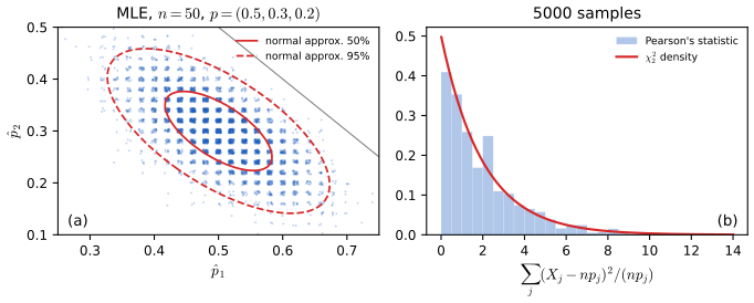
multinomial_draw (Exercise 3). (a) The MLE \((\widehat p_1,\widehat p_2)\) (slightly jittered; \(\widehat p_3\) is determined) and the 50% and 95% ellipses of its normal approximation \(\N(\bp,\bSigma/n)\) restricted to the first two coordinates (Theorem 14.6); the correlation is \(-p_1p_2/\sqrt{p_1(1-p_1)p_2(1-p_2)}\)\({}=-0.65\). (b) Pearson's statistic against \(\chi^2_2\) (Filling the gap 14.18). Code: fig_14_s5. Supplementary figure; illustrates Wasserman (2004), Theorems 14.4 and 14.6. Download: PDF · SVG14.5 Bibliographic Remarks
p. 237 The book recommends Johnson and Wichern and Anderson for multivariate analysis, and credits the interval for the correlation to Fisher (1921). The exact distribution of the sample correlation is Fisher (1915), and the form used in Filling the gap 14.7 is Hotelling (1953), which also refines Fisher's expansions; the \(T^2\) statistic is Hotelling (1931); the distribution of the sample covariance matrix is Wishart (1928). Anderson (2003) and Muirhead (1982) prove everything in Section 14.3 and much more (the Wishart density, the distribution of sample eigenvalues and of the correlation in many dimensions); Marchenko and Pastur (1967) is the source of the eigenvalue limits quoted in Filling the gap 14.14. The bootstrap intervals for the correlation are discussed by Efron and Tibshirani (1993).
14.6 Appendix
pp. 237–238 The appendix proves the expression for the log-likelihood in Theorem 14.3. Two slips in the printed proof (see the notes on the book) mean that, read literally, it arrives at the wrong trace term; here is the argument with them corrected.
Filling the gap 14.19: the normal log-likelihood through \((\Xbar,\bS)\) (proof of Theorem 14.3) pp. 237–238
Proof
The log-likelihood is the sum of the log densities (14.7):
\[ \ell(\bmu,\bSigma)=\sum_{i=1}^n\log f(\bX_i;\bmu,\bSigma)=-\frac{nk}2\log(2\pi)-\frac n2\log|\bSigma|-\frac12\sum_{i=1}^n(\bX_i-\bmu)^\T\bSigma^{-1}(\bX_i-\bmu). \]Split off the mean. With \(\bX_i-\bmu=(\bX_i-\Xbar)+(\Xbar-\bmu)\), the cross terms are \(2\sum_i(\bX_i-\Xbar)^\T\bSigma^{-1}(\Xbar-\bmu)\)\({}=0\), because \(\sum_i(\bX_i-\Xbar)=\bzero\). So
\[ \sum_i(\bX_i-\bmu)^\T\bSigma^{-1}(\bX_i-\bmu)=\sum_i(\bX_i-\Xbar)^\T\bSigma^{-1}(\bX_i-\Xbar)+n(\Xbar-\bmu)^\T\bSigma^{-1}(\Xbar-\bmu). \]The trace trick on the first sum. Each term is a scalar, so by Filling the gap 14.1(a),
\[ \sum_i(\bX_i-\Xbar)^\T\bSigma^{-1}(\bX_i-\Xbar)=\sum_i\tr\{\bSigma^{-1}(\bX_i-\Xbar)(\bX_i-\Xbar)^\T\}=\tr\Big\{\bSigma^{-1}\sum_i(\bX_i-\Xbar)(\bX_i-\Xbar)^\T\Big\}=(n-1)\tr(\bSigma^{-1}\bS). \]Putting the pieces together gives the statement of Theorem 14.3, with \(\frac{n-1}2\tr(\bSigma^{-1}\bS)\)\({}=\frac n2\tr(\bSigma^{-1}\hSigma)\). ∎
The book applies the trace step to \(\sum_i(\bX_i-\bmu)^\T\bSigma^{-1}(\bX_i-\bmu)\) and equates the result with \(n\tr(\bSigma^{-1}\bS)\); but \(\sum_i(\bX_i-\bmu)(\bX_i-\bmu)^\T\)\({}=(n-1)\bS+n(\Xbar-\bmu)(\Xbar-\bmu)^\T\) (Filling the gap 14.3), so the trace must be taken after the mean has been split off, and it produces \((n-1)\), not \(n\). That the corrected expression equals the direct sum of log densities, and the printed one does not, was confirmed numerically. The maximisation, which the appendix does not cover, is Filling the gap 14.10.
Notes on the book
Four slips of Chapter 14 are in the author's errata list (the first printing list); the other points are mine, each with the evidence.
Page 231: "\(\tr(AB)=\tr(BA)\) and \(\tr(A)+\tr(B)\)", and "A matrix is positive definite if \(x^T\Sigma x\gt0\)"
The second identity should read \(\tr(A+B)=\tr(A)+\tr(B)\), and the definition should name the matrix \(\Sigma\) that appears in it. Both are listed in the author's errata. The identities are proved in Filling the gap 14.1.
Page 233, (14.6): the numerator must be divided by \(n-1\); and the footnote
As printed, \(\hrho\)\({}=\sum_i(X_{1i}-\overline X_1)(X_{2i}-\overline X_2)/(s_1s_2)\) is \(n-1\) times the sample correlation and can exceed 1. Listed in the author's errata. The footnote then says the plug-in version (divisor \(n\)) differs slightly; once the formula is corrected, the two are identical, because the divisor cancels between numerator and denominator (Filling the gap 14.4(a)). Not in the errata lists.
Page 234: the standard error \(1/\sqrt{n-3}\) assumes normal data
Section 14.2 introduces \(\hrho\) as the nonparametric plug-in estimator, but the standard error \(1/\sqrt{n-3}\) of \(f(\hrho)\) is valid only when the data are bivariate normal (or have normal fourth moments). For elliptical data the asymptotic variance is \((1+\kappa)/n\) (Filling the gap 14.6), and Fisher's 95% interval covers only about 0.87 of the time for bivariate \(t_6\) data at \(n=100\) to 200 (Figure 14.S2(c); the limit is 0.834). The bootstrap, mentioned at the end of the section, does not have this problem. A remark on scope rather than an error; not in the errata lists.
Page 235, line 4 of Section 14.4: "balls of the \(k\)th color" should be "of the \(j\)th color"
Listed in the author's errata.
Page 235, Theorem 14.2, parts 1 and 2: \(\N(0,1)\) should be \(\N(\bzero,\bI)\)
\(\bSigma^{1/2}\bZ\) is a vector, so \(\bZ\) must be a vector of \(k\) independent standard normals, and \(\bSigma^{-1/2}(\bX-\bmu)\) likewise. Part 3 also lacks a comma after \(\N(\bmu,\bSigma)\). Not in the errata lists.
Page 235, Theorem 14.3: the trace term is \(\frac{n-1}2\tr(\bSigma^{-1}\bS)\), not \(\frac n2\tr(\bSigma^{-1}\bS)\)
With \(\bS\) defined with divisor \(n-1\) as in (14.4), the log-likelihood contains \(\frac12\sum_i(\bX_i-\Xbar)^\T\bSigma^{-1}(\bX_i-\Xbar)\)\({}=\frac{n-1}2\tr(\bSigma^{-1}\bS)\). Evidence: (1) the derivation of Filling the gap 14.19; (2) maximising the printed expression over \(\bSigma\) would give \(\bS\), not the \(\frac{n-1}n\bS\) that the same theorem states in (14.8), so the theorem contradicts itself; (3) numerically, for simulated data, the corrected expression equals the sum of the log densities to machine precision and the printed one does not. Not in the errata lists.
Pages 237–238, proof of Theorem 14.3
The first display writes \(\ell(\bmu,\bSigma)\)\({}=\sum_if(\bX_i;\bmu,\bSigma)\) for \(\sum_i\log f(\bX_i;\bmu,\bSigma)\). The final chain applies the trace identity to \(\sum_i(\bX_i-\bmu)^\T\bSigma^{-1}(\bX_i-\bmu)\) and ends with \(n\tr(\bSigma^{-1}\bS)\), which is false: the trace step should follow the decomposition, and it gives \((n-1)\tr(\bSigma^{-1}\bS)\). The proof also stops before maximising, so (14.8) is not proved there. Corrected in Filling the gap 14.19 and completed in Filling the gap 14.10. Not in the errata lists.
Pages 236–237: the Fisher information and Theorem 14.6 (remarks)
The proof of Theorem 14.5 finds a stationary point of the Lagrangian; it does not show that it is a maximum, and it divides by \(p_j\), which fails when a count is zero (Filling the gap 14.16 gives a complete argument). The "Fisher information matrix" mentioned after it exists only for \(k-1\) free parameters (Filling the gap 14.17), and the limit in Theorem 14.6 has the singular covariance \(\bSigma\), so it is not a normal law with a density (Filling the gap 14.18). Remarks on precision; not in the errata lists.
14.7 Exercises
All six exercises of Chapter 14 (Wasserman, 2004, p. 238), restated in my own words, with complete solutions (hidden). The computational ones are solved with the Python code.
Exercise 14.1. Prove Theorem 14.1.
Solution
See the proof under Theorem 14.1: linearity of expectation gives the means, and \(\V(\bA\bX)\)\({}=\E\{\bA(\bX-\bmu)(\bX-\bmu)^\T\bA^\T\}\)\({}=\bA\bSigma\bA^\T\) because expectation commutes with fixed linear maps of a random matrix. The vector statements are the case \(\bA=\ba^\T\) (a \(1\times k\) matrix). Note the immediate corollary that \(\ba^\T\bSigma\ba\ge0\) (Filling the gap 14.2).
Exercise 14.2. Find the Fisher information matrix of the multinomial model.
Solution
In the free parameters \(\btheta=(p_1,\dots,p_{k-1})\),
\[ I_n(\btheta)=n\Big\{\diag\big(\tfrac1{p_1},\dots,\tfrac1{p_{k-1}}\big)+\frac{\bone\bone^\T}{p_k}\Big\}, \]with inverse \((\diag\btheta-\btheta\btheta^\T)/n\), which equals \(\V(\widehat\btheta)\); see Filling the gap 14.17 for the derivation and for how \(\bSigma/n\) is recovered in all \(k\) coordinates. For \(k=2\) this is the binomial: \(I_n(p)=n\{1/p+1/(1-p)\}=n/\{p(1-p)\}\). The formula was also confirmed numerically, by finite differences of the expected log-likelihood and as the simulated covariance of the score.
Exercise 14.3 (computer experiment). Write a function that generates
nsimobservations from a \(\Mult(n,\bp)\) distribution.Solution
Method (
multinomial_draw): following Filling the gap 14.15, draw \(n\) uniforms per observation, turn each into a colour by finding the first \(j\) with \(U\le p_1+\dots+p_j\) (inverting the cumulative probabilities, as in inverse-CDF sampling), and count the colours. An alternative needing only \(k-1\) binomial draws per observation uses the conditional structure: \(X_1\sim\Bin(n,p_1)\), then \(X_2\given X_1\sim\Bin(n-X_1,p_2/(1-p_1))\), and so on. Confirmed numerically: for \(\bp=(0.5,0.3,0.2)\) and \(n=20\), 200000 draws have mean \(n\bp\) and covariance \(n\bSigma\) to within simulation error, \(X_1\) passes a goodness-of-fit test against \(\Bin(20,0.5)\), and the covariance agrees with numpy's sampler. Figure 14.S5 uses this function.Exercise 14.4 (computer experiment). Write a function that generates
nsimobservations from \(\N(\bmu,\bSigma)\) for a given \(\bmu\) and \(\bSigma\).Solution
Method (
mvn_draw): draw \(\bZ\) with independent \(\N(0,1)\) entries and return \(\bmu+\bB\bZ\) with \(\bB\bB^\T=\bSigma\). By Theorem 14.1 the result has mean \(\bmu\) and covariance \(\bB\bB^\T=\bSigma\), and by Filling the gap 14.8 it is normal. Two choices of \(\bB\) are implemented: the Cholesky factor (cheapest, the usual choice) and the symmetric square root \(\bSigma^{1/2}\) of Theorem 14.2(1), computed from the eigendecomposition. The two give different samples from the same distribution. Confirmed numerically: 500000 draws from \(\N\big((1,-1),\begin{pmatrix}2&-0.8\\-0.8&1\end{pmatrix}\big)\) reproduce the mean and covariance, and their Mahalanobis forms pass a test against \(\chi^2_2\) (Theorem 14.2(4)). The demonstrations use the Cholesky construction with the seeded generator of the pages.Exercise 14.5 (computer experiment). Generate 100 vectors from \(\N(\bmu,\bSigma)\) with \(\bmu=(3,8)^\T\) and \(\bSigma\)\({}=\begin{pmatrix}1&1\\1&2\end{pmatrix}\). Plot them, estimate \(\bmu\) and \(\bSigma\), find the true correlation and compare it with the sample correlation, and give 95% intervals for \(\rho\) by the bootstrap and by Fisher's method.
Solution
Method (
exercise5): 100 draws by the Cholesky construction; \(\Xbar\), \(\bS\) and \(\hSigma\) by (14.4) and (14.8); Fisher's interval as in the box above; the bootstrap percentile interval from 2000 resamples of the 100 pairs. The true correlation is \(\rho=1/\sqrt{1\cdot2}=0.7071\).quantity estimate truth \(\Xbar\) (3.107, 8.302) (3, 8) \(\bS\) entries \(s_{11},s_{12},s_{22}\) 0.954, 0.998, 2.090 1, 1, 2 \(\hSigma=\frac{99}{100}\bS\) 0.945, 0.988, 2.070 1, 1, 2 \(\hrho\) 0.7067 0.7071 Fisher 95% interval (0.5925, 0.7930) bootstrap percentile 95% interval (0.5936, 0.7969) delta-method interval \(\hrho\pm1.96(1-\hrho^2)/10\) (0.6086, 0.8048) The sample correlation is within 0.0004 of the truth here (its standard error is about \((1-\rho^2)/\sqrt n=0.05\), so this is luck). The Fisher and bootstrap intervals almost coincide, and both are asymmetric about \(\hrho\), reaching about 0.11 below it and 0.09 above it, reflecting the skewness of \(\hrho\) towards zero; the bootstrap standard error is 0.052, against 0.050 from the normal-theory formula. The delta-method interval is symmetric and shifted upwards. All three contain \(\rho\). Figure 14.S1 shows the sample with the true and estimated 95% ellipses, and the bootstrap distribution.
Exercise 14.6 (computer experiment). Repeat the previous exercise 1000 times and compare the coverage of the two intervals for \(\rho\).
Solution
Method (
corr_demo,exercise6_table): 1000 samples of 100 pairs, each with the Fisher interval, the bootstrap percentile interval (1000 resamples) and, for comparison, the delta-method interval; the experiment was repeated for \(n=10,\dots,200\) and for heavy-tailed data. Results for \(n=100\) (normal data): coverage 0.965 for Fisher, 0.954 for the bootstrap and 0.953 for the delta method; mean lengths 0.200, 0.196 and 0.196. With 1000 samples the Monte Carlo standard error of a coverage near 0.95 is 0.007, so all three are consistent with 0.95 at this \(n\); integrating the exact density of \(\hrho\) gives the exact coverages 0.950 (Fisher) and 0.939 (delta method). The differences appear at small \(n\) and under non-normality (Figure 14.S2):data \(n\) Fisher bootstrap delta method normal 10 0.952 0.909 0.847 normal 20 0.948 0.914 0.882 normal 100 0.965 0.954 0.953 \(t_{10}\) 100 0.917 0.943 0.915 \(t_6\) 100 0.874 0.945 0.868 \(t_6\) 200 0.863 0.940 0.864 Conclusions: for normal data Fisher's interval is the best at every sample size (it is almost exact even at \(n=10\), Filling the gap 14.7), and the bootstrap percentile interval undercovers when \(n\) is small (0.91 at \(n=10\) and 20), as percentile intervals typically do; the delta method is worst. For heavy-tailed data the ranking reverses: Fisher's interval keeps the normal-theory width while the true variability of \(z\) is \(1+\kappa\) times larger, so its coverage settles near \(2\Phi(1.96/\sqrt{1+\kappa})-1\) (0.910 for \(t_{10}\), 0.834 for \(t_6\)), while the bootstrap, which estimates the variance from the data, approaches 0.95.
Demonstrations for this chapter
Each demonstration runs in the browser, with exact computations and seeded random numbers, and links back to these notes. The ▶ Demo boxes above open them already set to the case under discussion. The numbers they show are the same as those of the Python code.
| Demonstration | What you can see | Sections and results |
|---|---|---|
| The sample correlation and Fisher's interval | The distribution of \(\hrho\) and of \(z\) over repeated samples, with the exact density, and the coverage and length of Fisher's, the bootstrap and the delta-method intervals, for normal or heavy-tailed data. Presets: 1 Exercise 6; 2 \(n=10\); 3 \(\rho\) near 1; 4 heavy tails; 5 \(\rho=0\). | 14.2; Fisher's interval, gaps 14.5–14.7; Exercise 6 |
| Hotelling's \(T^2\) against separate t-tests | Simulated t-statistics with the ellipse and the Bonferroni square, rejection rates, and power curves (exact for \(T^2\)) as the correlation, the sample size and the direction and length of the shift change. Presets: 1 sizes; 2 against the correlation; 3 along it; 4 independent coordinates; 5 \(n=5\). | Result 14.7, gaps 14.12, 14.13 |
| Conditioning a bivariate normal on a linear combination | A cloud of simulated points, a strip around \(\ba^\T\bx=c\) for \(\ba\) a coordinate, the sum or the difference, the histogram of the points in the strip against the exact conditional law, the line of conditional means and regression to the mean. Presets: 1 Exercise 5's distribution; 2 regression to the mean; 3 the reverse regression; 4 a sum; 5 a wide strip. | Theorem 14.2, gap 14.9 |
The Python code that produces every figure of this page is code/ch14_multivariate_models.py (see the code index).
References
- Wasserman, L. (2004). All of Statistics: A Concise Course in Statistical Inference. Springer, New York. Chapter 14, pp. 231–238. www.stat.cmu.edu/~larry/all-of-statistics.
- Anderson, T. W. (2003). An Introduction to Multivariate Statistical Analysis, 3rd edition. Wiley, Hoboken. (First edition 1958; the book cites the 1984 second edition.)
- Efron, B. and Tibshirani, R. J. (1993). An Introduction to the Bootstrap. Chapman and Hall, New York.
- Fisher, R. A. (1915). Frequency distribution of the values of the correlation coefficient in samples from an indefinitely large population. Biometrika, 10(4), 507–521.
- Fisher, R. A. (1921). On the "probable error" of a coefficient of correlation deduced from a small sample. Metron, 1, 3–32.
- Hotelling, H. (1931). The generalization of Student's ratio. Annals of Mathematical Statistics, 2(3), 360–378.
- Hotelling, H. (1953). New light on the correlation coefficient and its transforms. Journal of the Royal Statistical Society, Series B, 15(2), 193–232.
- Johnson, R. A. and Wichern, D. W. (2007). Applied Multivariate Statistical Analysis, 6th edition. Pearson Prentice Hall, Upper Saddle River. (The book cites the 1982 first edition.)
- Marchenko, V. A. and Pastur, L. A. (1967). Distribution of eigenvalues for some sets of random matrices. Mathematics of the USSR-Sbornik, 1(4), 457–483.
- Muirhead, R. J. (1982). Aspects of Multivariate Statistical Theory. Wiley, New York.
- Wishart, J. (1928). The generalised product moment distribution in samples from a normal multivariate population. Biometrika, 20A(1/2), 32–52.
The numerical statements in the text (the moments and density of the sample correlation and the expansions of the variance of \(z\), the exact and simulated coverages, the normal log-likelihood and its maximum, the Wishart moments and the law of \(T^2\), the power of the tests, the conditional laws, the multinomial moments, Fisher information and Pearson's statistic, and the answers to Exercises 5 and 6) were confirmed numerically.