Convergence of Random Variables
Statistics is about what happens as data accumulate, so it needs a language for the limits of random quantities. A sequence of random variables can approach a limit in several inequivalent ways: its distribution functions can converge, it can come close to the limit with high probability, its mean squared distance from the limit can vanish, or almost every one of its sample paths can converge. This chapter defines these modes, proves which imply which and refutes the rest, and then proves the two results the rest of the course leans on: the law of large numbers (averages settle at the mean) and the central limit theorem (their fluctuations are approximately normal). Slutsky's theorem, the continuous mapping theorem and the delta method then carry these limits through the transformations that every estimator involves.
Ch. 1 Probability Ch. 2 Random variables Ch. 3 Expectation Ch. 4 Inequalities Ch. 5 Convergence Ch. 6 Models and inference Ch. 7 Estimating the CDF Ch. 8 Bootstrap Ch. 9 Parametric inference Ch. 10 Hypothesis testing Ch. 11 Bayesian inference Ch. 12 Decision theory Ch. 13 Regression Ch. 14 Multivariate models Ch. 15 Independence Ch. 16 Causal inference Ch. 17 Directed graphs Ch. 18 Undirected graphs Ch. 19 Log-linear models Ch. 20 Curve estimation Ch. 21 Orthogonal functions Ch. 22 Classification Ch. 23 Stochastic processes Ch. 24 Simulation
How to read these notes
They follow the book. Sections carry the book's numbers (5.2, 5.7.1, ...), definitions and theorems keep the book's numbers (Definition 5.1, Theorem 5.4, ...), and the book's numbered equations (5.1)–(5.4) keep their numbers, so you can read these notes next to the book.
Filling the gaps. The book states many results of this chapter without proof (Theorem 5.5, the central limit theorem with only a finite variance, Theorems 5.10–5.12, 5.15, 5.17–5.19 and Lemma 5.20). Each gets a complete proof here, in an orange Filling the gap box, or a careful sketch with a reference where a full proof would need machinery beyond the course (the Berry–Esseen constant). Proofs start hidden: open one with its bar, or use the button below.
Figures and demonstrations. Figure 5.1 is reproduced from scratch by the Python code; Figure 5.2, a diagram, is redrawn and extended; six supplementary figures (5.S1–5.S6) show results the book states without a picture. The ▶ Demo boxes open an interactive demonstration already set to the case being discussed.
Main reference
L. Wasserman, All of Statistics: A Concise Course in Statistical Inference, Springer (2004), Chapter 5, pages 71–84 (book website: www.stat.cmu.edu/~larry/all-of-statistics). Section, theorem, equation, figure and exercise numbers below refer to this book. Further reading is listed in the references.
The explanations, derivations, figures and code are my own; results and equations are cited by their numbers in the book.
Companion courses
The law of large numbers, the central limit theorem and the delta method appear, at other levels, in the other courses on this site. The overlapping material is:
- Section 5.3 (Markov and Chebyshev, the weak law): the first-year notes, Section 0.3, Theorem 0.4 and Theorem 0.5; Foundations of Deep Learning, Filling the gap 2.3 (why a sample average approximates an expectation).
- Section 5.4 (the central limit theorem): the first-year notes, Section 0.5 and Theorem 0.7 (a moment generating function sketch), with the central limit theorem demo; Foundations of Deep Learning, Filling the gap 3.1 (a characteristic function sketch); Bayesian and Probabilistic Machine Learning, Section 2.3.
- Theorem 5.10 (the CLT with an estimated variance): the large-sample interval of the first-year notes, Theorem 3.5.
- Section 5.5 (the delta method): Statistical Methods for Modern Biology, Filling the gap 3.16 and Result 3.7 (variance-stabilising transformations), with the variance-stabilisation demo.
- Convergence in quadratic mean in action: the Robbins–Monro algorithm, Result 2.15 of Bayesian and Probabilistic Machine Learning.
Those courses state the central limit theorem and sketch it; here every step is proved under a finite variance alone (Filling the gap 5.7). New here: the full map of the five modes of convergence with a counterexample for every non-implication, the portmanteau characterisation, complete proofs of Slutsky's theorem and the continuous mapping theorem, the weak law with only a finite mean, the multivariate central limit theorem and delta method, the second-order delta method, the Borel–Cantelli lemmas, Etemadi's proof of the strong law, uniform integrability, the Berry–Esseen constants with exact computations, and seven notes on the book (listed in Notes on the book).
The chapter at a glance
- 5.2 Convergence in probability, in distribution (Definition 5.1) and in quadratic mean (Definition 5.2); quadratic mean \(\Rightarrow\) probability \(\Rightarrow\) distribution, and distribution \(\Rightarrow\) probability for a constant limit (Theorem 5.4); a counterexample for every other arrow (Filling the gap 5.2). Sums, products and continuous functions preserve the limits (Theorem 5.5, proved in Filling the gap 5.4).
- 5.3 The weak law of large numbers (Theorem 5.6), by Chebyshev with a finite variance and by truncation with a finite mean (Filling the gap 5.5).
- 5.4 The central limit theorem (Theorem 5.8, proved in Filling the gap 5.7), with an estimated variance (Theorem 5.10), its rate (Theorem 5.11, Berry–Esseen) and in several dimensions (Theorem 5.12).
- 5.5 The delta method in one (Theorem 5.13) and several (Theorem 5.15) dimensions, and what happens when the derivative vanishes (Filling the gap 5.11).
- 5.7 Almost-sure and \(L^1\) convergence (Theorem 5.17), the Borel–Cantelli lemmas, the strong law (Theorem 5.18, proved in Filling the gap 5.14), uniform integrability (Theorem 5.19) and the moment generating function route to the central limit theorem (Lemma 5.20).
Notation. \(X_1,X_2,\dots\) random variables on one probability space \((\Omega,\mathcal A,\P)\), with cdfs \(F_n\); \(X\) another random variable with cdf \(F\). \(\Xb=n^{-1}\sum_{i=1}^nX_i\) is the sample mean, \(\mu=\E X_1\), \(\sigma^2=\V X_1\), \(S_n^2\)
Prerequisites. Expectation, variance and independence (Chapters 2–3 of the book), Markov's and Chebyshev's inequalities (Chapter 4), Taylor's theorem with remainder, and the continuity of a probability measure along monotone sequences of events (Chapter 1).
5.1 Introduction
pp. 71–72 For numbers, \(x_n\to x\) means that for every \(\eps>0\), \(|x_n-x|<\eps\) for all large \(n\). Two examples show why random variables need something else. If \(X_1,X_2,\dots\) are independent \(N(0,1)\), every \(X_n\) has the same distribution as a fixed \(X\sim N(0,1)\), yet \(\P(X_n=X)=0\): the variables do not approach anything, only their distributions agree. If \(X_n\sim N(0,1/n)\), the distribution piles up at 0, yet \(\P(X_n=0)=0\) for every \(n\). The chapter's answer is to measure closeness in several ways, each suited to a different purpose, and its two headline results are
- the law of large numbers: \(\Xb\) converges in probability to \(\mu=\E X_1\), so the sample mean is close to the population mean with high probability;
- the central limit theorem: \(\sqrt n(\Xb-\mu)\) converges in distribution to a normal law, so probabilities about \(\Xb\) can be computed from a normal distribution.
5.2 Types of Convergence
Definition 5.1 (convergence in probability and in distribution) p. 72, (5.1)–(5.2)
(1) \(X_n\) converges to \(X\) in probability, written \(X_n\cP X\), if for every \(\eps>0\)
\[ \P(|X_n-X|>\eps)\to0\quad\text{as }n\to\infty. \tag{5.1} \](2) \(X_n\) converges to \(X\) in distribution, written \(X_n\cd X\), if
\[ \lim_{n\to\infty}F_n(t)=F(t)\quad\text{at every }t\text{ at which }F\text{ is continuous}. \tag{5.2} \]When \(\P(X=c)=1\) we write \(X_n\cP c\) and \(X_n\cd c\).
The two definitions are of different kinds. Convergence in probability compares the random variables \(X_n(\omega)\) and \(X(\omega)\) on the same sample point, so it needs all of them on one probability space. Convergence in distribution only compares the cdfs; \(X_n\) and \(X\) could live on different spaces, and the statement is really about the laws.
Definition 5.2 (convergence in quadratic mean) p. 73, (5.3)
\(X_n\) converges to \(X\) in quadratic mean (or in \(L^2\)), written \(X_n\cqm X\), if
\[ \E(X_n-X)^2\to0\quad\text{as }n\to\infty. \tag{5.3} \]Example 5.3. p. 73 Let \(X_n\sim N(0,1/n)\) and let \(F\) be the cdf of the point mass at 0. Since \(\sqrt nX_n\sim N(0,1)\), \(F_n(t)=\Phi(\sqrt n\,t)\), which tends to 0 for \(t<0\) and to 1 for \(t>0\). So \(F_n(t)\to F(t)\) for every \(t\ne0\), and \(X_n\cd0\), although \(F_n(0)=\tfrac12\ne F(0)=1\) for every \(n\). Also, by Chebyshev's inequality, \(\P(|X_n|>\eps)\)
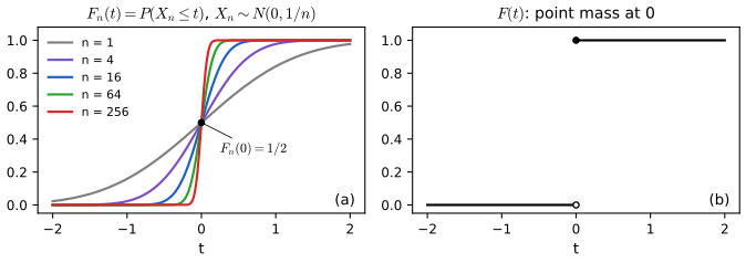
fig_5_1. Reproduces Wasserman (2004), Figure 5.1. Download: PDF · SVGFilling the gap 5.1: why only the continuity points, and why that is enough pp. 72–73
(a) Requiring \(F_n(t)\to F(t)\) at every \(t\) would make Example 5.3 fail, and would even make \(X_n=1/n\) fail to converge to 0. (b) The exemption costs nothing: a cdf has at most countably many jumps, its continuity points are dense, and a cdf is determined by its values on any dense set; so the limit law in (5.2) is unique.
Proof
(a) For \(X_n=1/n\) (a constant), \(F_n(0)=\P(1/n\le0)=0\) for every \(n\), while the point mass at 0 has \(F(0)=1\). A definition that demanded convergence at \(t=0\) would deny that \(1/n\to0\), which no sensible notion of convergence can do. The trouble is only at the jump of the limit.
(b) For each \(k\ge1\), the set of points where \(F\) jumps by more than \(1/k\) has at most \(k\) elements, since the jumps add up to at most 1. The set of all jumps is the union over \(k\) of these finite sets, hence countable, and its complement is dense. Now suppose \(F\) and \(G\) are cdfs that agree on a dense set \(D\). For any \(t\), choose \(t_j\in D\), \(t_j\downarrow t\); right-continuity gives \(F(t)\)
The relations between the modes
Theorem 5.4 (relations between the modes of convergence) p. 73
(a) \(X_n\cqm X\) implies \(X_n\cP X\). (b) \(X_n\cP X\) implies \(X_n\cd X\). (c) If \(X_n\cd X\) and \(\P(X=c)=1\) for a constant \(c\), then \(X_n\cP X\). In general no other implication holds.
Proof
(a) By Markov's inequality applied to \(|X_n-X|^2\), \(\P(|X_n-X|>\eps)\)
(b) Fix \(\eps>0\) and a continuity point \(x\) of \(F\). If \(X_n\le x\) then either \(X\le x+\eps\) or \(|X_n-X|>\eps\); if \(X\le x-\eps\) then either \(X_n\le x\) or \(|X_n-X|>\eps\). Hence
\[ F(x-\eps)-\P(|X_n-X|>\eps)\le F_n(x)\le F(x+\eps)+\P(|X_n-X|>\eps). \]Letting \(n\to\infty\), \(F(x-\eps)\)
(c) The limit cdf is \(F(t)=\I(t\ge c)\), continuous everywhere except at \(c\). For \(\eps>0\), \(c-\eps\) and \(c+\eps\) are continuity points, so
\[ \P(|X_n-c|>\eps)\le F_n(c-\eps)+1-F_n(c+\eps)\to F(c-\eps)+1-F(c+\eps)=0+1-1=0. \]That the remaining implications fail is the content of the next box. ∎
Filling the gap 5.2: a counterexample for every missing arrow pp. 74–75
Let \(U\sim\) Uniform(0,1) and consider the spikes \(X_n=n^a\I(U<n^{-b})\) with \(a\ge0\), \(b>0\), and the sequence \(X_n=-X\) with \(X\sim N(0,1)\). Then
| sequence | limit | distribution | probability | \(L^1\) | quadratic mean | almost surely |
|---|---|---|---|---|---|---|
| \(\sqrt n\,\I(U<1/n)\) (the book's) | 0 | yes | yes | yes | no | yes |
| \(n^2\,\I(U<1/n)\) (the warning) | 0 | yes | yes | no | no | yes |
| \(n^{3/4}\,\I(U<1/n)\) | 0 | yes | yes | yes | no | yes |
| \(\I(U_n<1/n)\), \(U_n\) independent | 0 | yes | yes | yes | yes | no |
| \(-X\), \(X\sim N(0,1)\) | \(X\) | yes | no | no | no | no |
So probability does not imply quadratic mean or \(L^1\) (rows 1–2), \(L^1\) does not imply quadratic mean (row 3), almost-sure convergence does not imply \(L^1\) (row 2), quadratic mean does not imply almost-sure convergence (row 4), and distribution does not imply probability (row 5). Convergence in probability does not even make the means converge: in row 2, \(\E X_n=n\to\infty\) (the book's warning, p. 75).
Proof
Spikes with one \(U\). \(X_n\ne0\) exactly when \(U<n^{-b}\), so \(\P(|X_n|>\eps)\)
Independent spikes (row 4). \(X_n=\I(U_n<1/n)\) has \(\E X_n=\E X_n^2=1/n\to0\). But the events \(A_n=\{X_n=1\}\) are independent with \(\sum_n\P(A_n)=\sum1/n=\infty\), so by the second Borel–Cantelli lemma (Filling the gap 5.13) infinitely many of them occur with probability 1: almost every path keeps returning to 1, and \(X_n\) converges almost surely to nothing. The marginal laws of rows 1–4 depend only on \(a\) and \(b\); whether the paths converge depends on the joint law of the sequence. That is why almost-sure convergence is the only mode in the table that is not determined by the individual laws of the \(X_n-X\).
Row 5. \(-X\sim N(0,1)\) by symmetry, so \(F_n=F\) for every \(n\) and \(X_n\cd X\) trivially. But \(|X_n-X|=2|X|\) for every \(n\), so \(\P(|X_n-X|>\eps)\)
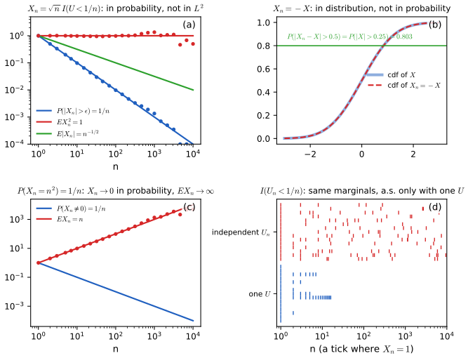
fig_5_s1. Download: PDF · SVGPreserving convergence under transformations
Theorem 5.5 (sums, products and continuous maps; Slutsky's theorem) p. 75
Let \(g\) be continuous. Then
(a) \(X_n\cP X\) and \(Y_n\cP Y\) imply \(X_n+Y_n\cP X+Y\);
(b) \(X_n\cqm X\) and \(Y_n\cqm Y\) imply \(X_n+Y_n\cqm X+Y\);
(c) \(X_n\cd X\) and \(Y_n\cd c\) imply \(X_n+Y_n\cd X+c\);
(d) \(X_n\cP X\) and \(Y_n\cP Y\) imply \(X_nY_n\cP XY\);
(e) \(X_n\cd X\) and \(Y_n\cd c\) imply \(X_nY_n\cd cX\);
(f) \(X_n\cP X\) implies \(g(X_n)\cP g(X)\);
(g) \(X_n\cd X\) implies \(g(X_n)\cd g(X)\).
(c) and (e) are Slutsky's theorem (Slutsky 1925); (f) and (g) are the continuous mapping theorem (Mann and Wald 1943). \(X_n\cd X\) and \(Y_n\cd Y\) do not imply \(X_n+Y_n\cd X+Y\) (Exercise 5.16).
The book states Theorem 5.5 without proof. The proofs rest on two facts about convergence in distribution, proved first.
Filling the gap 5.3: tightness, and convergence in distribution through test functions
(T) Tightness. If \(X_n\cd X\), then for every \(\eta>0\) there is \(M\) with \(\P(|X_n|>M)<\eta\) for all \(n\) (the sequence is bounded in probability).
(P) Portmanteau. \(X_n\cd X\) if and only if \(\E f(X_n)\to\E f(X)\) for every bounded continuous \(f:\R\to\R\). In the "if" direction it is enough that this holds for every \(f\) with three bounded continuous derivatives.
Proof
(T). Choose \(M_0>0\) with \(\pm M_0\) continuity points of \(F\) (possible: the discontinuities are countable) and \(F(-M_0)<\eta/4\), \(1-F(M_0)<\eta/4\). Since \(F_n(\pm M_0)\to F(\pm M_0)\), there is \(n_0\) such that for \(n\ge n_0\), \(\P(|X_n|>M_0)\)
(P), "only if". Let \(|f|\le K\) and \(\eps>0\). By (T) and the countability of the jumps of \(F\), pick continuity points \(-M\) and \(M\) of \(F\) with \(\P(|X|>M)<\eps\) and \(\P(|X_n|>M)<\eps\) for all \(n\). \(f\) is uniformly continuous on \([-M,M]\), so there are continuity points \(-M=a_0<a_1\)
(P), "if". Fix a continuity point \(t\) of \(F\) and \(\delta>0\). Let \(s(u)=35u^4-84u^5+70u^6-20u^7\) for \(u\in[0,1]\), \(s=0\) for \(u<0\), \(s=1\) for \(u>1\); \(s\) increases from 0 to 1, and its first three derivatives vanish at 0 and 1, so \(s\) has three bounded continuous derivatives. The function \(f(x)=1-s((x-t)/\delta)\) satisfies \(\I(x\le t)\)
so \(F(t-\delta)\)
Filling the gap 5.4: proof of Theorem 5.5 p. 75
All seven parts follow from Markov's inequality, the tightness fact (T) and the portmanteau fact (P) of Filling the gap 5.3, and two small lemmas: (L1) if \(U_n\cP0\) and \(V_n\) is bounded in probability then \(U_nV_n\cP0\); (L2) if \(g\) is continuous at every point and \(X\) is a random variable, then for every \(\eps,\eta>0\) there is \(\delta>0\) with \(\P(|g(X+h)-g(X)|\ge\eps\text{ for some }|h|<\delta)\)
Proof
(L1). Given \(\eps,\eta\), take \(M\) with \(\P(|V_n|>M)<\eta\) for all \(n\); then \(\P(|U_nV_n|>\eps)\)
(L2). Choose \(M\) with \(\P(|X|>M)<\eta\). \(g\) is uniformly continuous on \([-M-1,M+1]\): there is \(\delta\in(0,1)\) with \(|g(x+h)-g(x)|<\eps\) whenever \(|x|\le M\) and \(|h|<\delta\). So the event in (L2) is contained in \(\{|X|>M\}\).
(a) \(|X_n+Y_n-X-Y|\)
(b) \((u+v)^2\le2u^2+2v^2\) gives \(\E(X_n+Y_n-X-Y)^2\)
(c) By Theorem 5.4(c), \(Y_n\cP c\). Let \(t\) be a point with \(t-c\) a continuity point of \(F\), and \(\eps>0\) with \(t-c\pm\eps\) also continuity points. Then
\[ \P(X_n\le t-c-\eps)-\P(|Y_n-c|>\eps)\le\P(X_n+Y_n\le t)\le\P(X_n\le t-c+\eps)+\P(|Y_n-c|>\eps), \]so \(F(t-c-\eps)\)
(d) Decompose the difference as
\[ X_nY_n-XY=(X_n-X)(Y_n-Y)+X(Y_n-Y)+Y(X_n-X). \]The last two terms tend to 0 in probability by (L1) with \(V=X\) or \(Y\); the first because \(\P(|U_nV_n|>\eps)\)
(e) Write \(X_nY_n=cX_n+X_n(Y_n-c)\). The second term tends to 0 in probability by (L1) (\(X_n\) is bounded in probability by (T)). \(cX_n\cd cX\) by (g) below with \(g(x)=cx\). Then (c) with the constant 0 gives \(X_nY_n\cd cX\).
(f) Given \(\eps,\eta\), take \(\delta\) from (L2). Then \(\P(|g(X_n)-g(X)|\ge\eps)\)
(g) For bounded continuous \(f\), \(f\circ g\) is bounded and continuous, so by (P) \(\E f(g(X_n))\to\E f(g(X))\); by (P) again, \(g(X_n)\cd g(X)\).
The same statements in \(\R^k\). With \(|\cdot|\) the Euclidean norm, (a), (b), (d), (f), (T), (L1), (L2) and (P) hold for random vectors with the same proofs (in (P) and (T) use products of the one-dimensional smooth steps, and multivariate cdfs at continuity points). They are used in Section 5.5. ∎
5.3 The Law of Large Numbers
p. 76 Let \(X_1,X_2,\dots\) be iid with mean \(\mu\) and variance \(\sigma^2\). The sample mean has \(\E\Xb=\mu\) and \(\V\Xb=\sigma^2/n\).
See also: the first-year notes, Theorem 0.5; Foundations of Deep Learning, Filling the gap 2.3.
Theorem 5.6 (the weak law of large numbers) p. 76
If \(X_1,\dots,X_n\) are iid with \(\E|X_1|<\infty\), then \(\Xb\cP\mu\).
Proof with a finite variance
By Chebyshev's inequality, \(\P(|\Xb-\mu|>\eps)\)
Filling the gap 5.5: the weak law with only a finite mean p. 76
If the \(X_i\) are iid with \(\E|X_1|<\infty\) (the variance may be infinite), then \(\Xb\cP\mu\).
Proof (truncation)
Fix \(M>0\) and split each observation into a bounded part and a tail: \(X_i=U_i+W_i\) with \(U_i=X_i\I(|X_i|\le M)\), \(W_i=X_i\I(|X_i|>M)\). Then
\[ \Xb-\mu=(\overline U_n-\E U_1)+(\overline W_n-\E W_1). \]The bounded part has variance at most \(\E U_1^2\le M^2\), so by Chebyshev \(\P(|\overline U_n-\E U_1|>\eps)\)
Let \(n\to\infty\): \(\limsup_n\P(|\Xb-\mu|>2\eps)\)
Without a finite mean the law can fail completely: for Cauchy observations \(\Xb\) is again standard Cauchy for every \(n\) (its characteristic function is \(e^{-|t|}\), and \((e^{-|t|/n})^n=e^{-|t|}\)), so it does not concentrate at all (Figure 5.S6).
Example 5.7. p. 76 Toss a coin with \(\P(\text{heads})=p=\tfrac12\) and let \(\Xb\) be the fraction of heads. How many tosses make \(\P(0.4\le\Xb\le0.6)\ge0.7\)? Since \(\V\Xb=1/(4n)\), Chebyshev gives \(\P(|\Xb-\tfrac12|\le0.1)\)
Filling the gap 5.6: how conservative is Chebyshev in Example 5.7? p. 76
The exact answer is far smaller. The binomial probability \(\P(0.4\le\Xb\le0.6)\) first reaches 0.7 at \(n=20\) (0.737), then dips below 0.7 again at some odd and even \(n\) because of the lattice, and stays at or above 0.7 for every \(n\ge29\). The normal approximation \(2\Phi(0.2\sqrt n)-1\ge0.7\) gives \(n\ge27\).
Derivation
\(n\Xb\sim\) Binomial\((n,\tfrac12)\) and the event is \(\lceil0.4n\rceil\)coin_interval_prob). It is not monotone in \(n\): the number of integers in \([0.4n,0.6n]\) changes by 0, 1 or 2 from one \(n\) to the next. Examples: \(n=20\): 0.737; \(n=21\): 0.617; \(n=28\): 0.655; \(n=29\): 0.735, and every larger \(n\) gives at least 0.70. For the normal approximation, \(\P(|\Xb-\tfrac12|\le0.1)\)
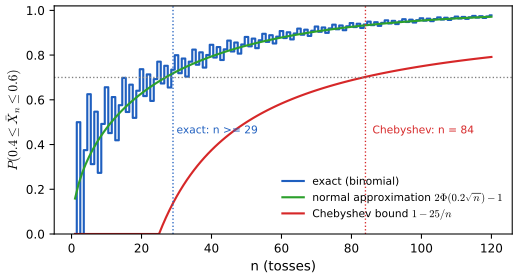
fig_5_s2. Download: PDF · SVGThe law of large numbers says that the distribution of \(\Xb\) concentrates at \(\mu\); it does not say that \(\Xb\) equals \(\mu\), nor how fast it concentrates beyond Chebyshev's \(1/n\). The stronger statement that almost every sequence of averages converges is the strong law of the appendix (Theorem 5.18).
5.4 The Central Limit Theorem
pp. 77–78 The law of large numbers says where \(\Xb\) goes; the central limit theorem describes the fluctuations around it, on the scale \(\sigma/\sqrt n\).
See also: the first-year notes, Theorem 0.7 and the CLT demo; Foundations of Deep Learning, Filling the gap 3.1. Both give a transform-based sketch; the proof below needs no transform.
Theorem 5.8 (the central limit theorem) p. 77
Let \(X_1,\dots,X_n\) be iid with mean \(\mu\) and variance \(\sigma^2\in(0,\infty)\). Then
\[ Z_n=\frac{\Xb-\mu}{\sqrt{\V(\Xb)}}=\frac{\sqrt n(\Xb-\mu)}{\sigma}\cd Z\sim N(0,1),\qquad\text{i.e.}\quad\lim_{n\to\infty}\P(Z_n\le z)=\Phi(z)\ \text{ for all }z. \]The book's interpretation is worth keeping: what is approximated are probability statements about \(\Xb\), not \(\Xb\) itself. The equivalent shorthands \(Z_n\approx N(0,1)\), \(\Xb\approx N(\mu,\sigma^2/n)\), \(\sqrt n(\Xb-\mu)\)
Filling the gap 5.7: a complete proof of the central limit theorem (Lindeberg's replacement method) pp. 77, 81–82
The book proves Theorem 5.8 in the appendix assuming that the moment generating function exists near 0 and quoting Lemma 5.20 without proof (both are completed in Filling the gap 5.16). Here is a proof that uses only \(\sigma^2<\infty\). It also gives a rate: if \(\rho=\E|X_1-\mu|^3<\infty\) and \(f\) has three bounded continuous derivatives,
\[ \big|\E f(Z_n)-\E f(Z)\big|\le\frac{\|f'''\|_\infty}{6\sqrt n}\Big(\frac{\rho}{\sigma^3}+\E|Z|^3\Big),\qquad\E|Z|^3=2\sqrt{2/\pi}\approx1.596. \]Proof
Set-up. Let \(Y_i=(X_i-\mu)/\sigma\), so \(\E Y_i=0\), \(\E Y_i^2=1\) and \(Z_n=n^{-1/2}\sum_{i=1}^nY_i\). On the same space take \(W_1,\dots,W_n\) iid \(N(0,1)\), independent of the \(Y\)'s; then \(n^{-1/2}\sum W_i\sim N(0,1)\) has the law of \(Z\). By the portmanteau fact (P) of Filling the gap 5.3 it suffices to show \(\E f(Z_n)\to\E f(Z)\) for every \(f\) with three bounded continuous derivatives.
Replacing one variable at a time. For \(k=0,\dots,n\) let
\[ S_k=n^{-1/2}(Y_1+\dots+Y_k+W_{k+1}+\dots+W_n), \]so \(S_n=Z_n\) and \(S_0\) has the law of \(Z\). With
\[ T_k=n^{-1/2}(Y_1+\dots+Y_{k-1}+W_{k+1}+\dots+W_n) \]we have \(S_k=T_k+Y_k/\sqrt n\), \(S_{k-1}=T_k+W_k/\sqrt n\), and
\[ \E f(Z_n)-\E f(Z)=\sum_{k=1}^n\Big\{\E f\big(T_k+\tfrac{Y_k}{\sqrt n}\big)-\E f\big(T_k+\tfrac{W_k}{\sqrt n}\big)\Big\}. \]Taylor. For real \(t,h\), \(f(t+h)=f(t)\)
where the last step only bounds each term by the same quantity (the bounds on \(R\) do not depend on \(t\)).
The remainder vanishes. Fix \(\eps>0\). On \(\{|Y_1|\le\eps\sqrt n\}\) use the cubic bound, elsewhere the quadratic one:
\[ n\,\E\big|R\big(T,\tfrac{Y_1}{\sqrt n}\big)\big|\le n\Big\{\frac{\|f'''\|}{6}\frac{\eps\sqrt n\,\E Y_1^2}{n^{3/2}}+\|f''\|\frac{\E[Y_1^2\I(|Y_1|>\eps\sqrt n)]}{n}\Big\}=\frac{\|f'''\|\eps}{6}+\|f''\|\,\E[Y_1^2\I(|Y_1|>\eps\sqrt n)]. \]The last expectation tends to 0 as \(n\to\infty\) by dominated convergence (\(\E Y_1^2<\infty\)). The same bound holds for \(W_1\). Hence \(\limsup_n|\E f(Z_n)-\E f(Z)|\)
The rate. If \(\E|Y_1|^3\)
Example 5.9. pp. 77–78 The number of errors in a program is Poisson with mean 5; for 125 programs, \(\P(\Xb<5.5)\)
The variance is rarely known. Estimate it by \(S_n^2\):
Theorem 5.10 (the CLT with an estimated variance) p. 78
Under the conditions of Theorem 5.8, \(\sqrt n(\Xb-\mu)/S_n\cd N(0,1)\).
Filling the gap 5.8: proof of Theorem 5.10 p. 78
The book states the result without proof. It is Slutsky's theorem applied to \(\sigma/S_n\cP1\).
Proof
By Exercise 5.1(b), \(S_n^2\cP\sigma^2\) (only a finite variance is needed: the weak law applies to \(X_i^2\), which has finite mean). The map \(x\mapsto\sigma/\sqrt{x}\) is continuous on \((0,\infty)\) and \(\sigma^2>0\), so by the continuous mapping theorem (Theorem 5.5(f), in the version for functions continuous at the limit, which has the same proof) \(\sigma/S_n\cP1\) (set it to 0 on the event \(S_n=0\), whose probability tends to 0). Then
\[ \frac{\sqrt n(\Xb-\mu)}{S_n}=\frac{\sigma}{S_n}\cdot\frac{\sqrt n(\Xb-\mu)}{\sigma}\cd1\cdot Z \]by Theorem 5.8 and Slutsky's theorem 5.5(e). ∎
This is why the large-sample interval \(\Xb\pm z_{\alpha/2}S_n/\sqrt n\) has asymptotic coverage \(1-\alpha\) whatever the shape of the distribution (first-year notes, Theorem 3.5). For normal data the exact law of the ratio is Student's \(t_{n-1}\), which tends to \(N(0,1)\) consistently with the theorem.
Theorem 5.11 (the Berry–Esseen inequality) p. 78, (5.4)
If \(\E|X_1|^3<\infty\), then
\[ \sup_z\big|\P(Z_n\le z)-\Phi(z)\big|\le\frac{33}{4}\,\frac{\E|X_1-\mu|^3}{\sqrt n\,\sigma^3}. \tag{5.4} \]Filling the gap 5.9: the Berry–Esseen theorem, its constant, and what the error looks like p. 78
(a) The constant. (5.4) holds with \(33/4\) in place of a universal constant \(C\); the theorem is due to Berry (1941) and Esseen (1942). The smallest valid \(C\) is not known exactly: \(C\le0.4748\) (Shevtsova 2011), and \(C\)
(b) The rate \(n^{-1/2}\) cannot be improved. For Bernoulli\((\tfrac12)\) observations, \(\sqrt n\,\sup_z|\P(Z_n\le z)-\Phi(z)|\)
(c) The shape of the error. For a non-lattice law with skewness \(\gamma=\E(X_1-\mu)^3/\sigma^3\), \(\P(Z_n\le z)\)
Proof sketch and computations
(a): how the theorem is proved. Two ingredients, both in Feller (1971, Section XVI.5). The first is Esseen's smoothing inequality: if \(G\) has a density bounded by \(m\), then for any cdf \(F\) and any \(T>0\), \[ \sup_z|F(z)-G(z)|\le\frac1\pi\int_{-T}^T\Big|\frac{\varphi_F(t)-\varphi_G(t)}{t}\Big|\d t+\frac{24m}{\pi T}, \] where \(\varphi\) are characteristic functions. It converts closeness of characteristic functions near the origin into closeness of cdfs. The second is a bound on the characteristic function of \(Z_n\): for \(|t|\le\sigma^3\sqrt n/(4\rho)\), \(|\varphi_{Z_n}(t)-e^{-t^2/2}|\)
(b): the lattice lower bound. For Bernoulli\((\tfrac12)\) and even \(n\), \(Z_n\) has an atom at 0 of probability \(\binom{n}{n/2}2^{-n}\)
Exact computations (Figure 5.S3). For gamma, Bernoulli and Poisson observations \(S_n\) is gamma, binomial or Poisson, so \(d_n\)ks_exact. The constant each law needs, \(d_n\sqrt n\sigma^3/\rho\), is about 0.055 for the exponential (\(\rho/\sigma^3=12/e-2\)), 0.06 for Gamma\((\tfrac14)\), 0.15 for Poisson(1) and 0.40 for Bernoulli\((\tfrac12)\): the lattice laws are the hard cases, and none comes close to \(33/4\). The one-term Edgeworth expansion of (c) leaves an error of order \(1/n\) (0.0080 at \(n=10\) for the exponential, against \(d_{10}=0.042\)); Esseen's sawtooth term does the same for the lattice laws (for Bernoulli\((\tfrac12)\) the error falls from 0.040 to 0.0012 at \(n=100\)). Where (c) comes from: expanding \(\log\varphi_{Z_n}(t)\)
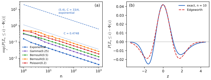
fig_5_s3. Download: PDF · SVGTheorem 5.12 (the multivariate central limit theorem) pp. 78–79
Let \(X_1,\dots,X_n\) be iid random vectors in \(\R^k\) with mean \(\mu\) and covariance matrix \(\Sigma\) (finite). Let \(\overline X=n^{-1}\sum_iX_i\), the vector of the \(k\) coordinate means. Then \(\sqrt n(\overline X-\mu)\)
Filling the gap 5.10: proof of the multivariate central limit theorem p. 79
For random vectors, \(V_n\cd V\) means that the joint cdfs \(F_n(t)=\P(V_n\le t)\) (componentwise inequality) converge at every continuity point of \(F\). The book states Theorem 5.12 without proof; Lindeberg's argument of Filling the gap 5.7 carries over word for word.
Proof
Let \(Y_i=X_i-\mu\) and \(W_i\sim N(0,\Sigma)\) iid, independent of the \(Y\)'s; \(n^{-1/2}\sum W_i\)
To pass to cdfs, take \(f(x)=\prod_{j=1}^kf_j(x_j)\), with \(f_j\) the smooth steps of Filling the gap 5.3 at \(t_j\) and \(t_j+\delta\) (or \(t_j-\delta\) and \(t_j\)): \(\I(x\le t)\)
An equivalent route is the Cramér–Wold device (Cramér and Wold 1936): \(V_n\cd V\) in \(\R^k\) iff \(a^\T V_n\cd a^\T V\) for every \(a\in\R^k\). With it, Theorem 5.12 follows from the one-dimensional CLT applied to \(a^\T X_i\), which has variance \(a^\T\Sigma a\). Its proof needs characteristic functions (Lévy's continuity theorem), which is why the direct argument is given here.
5.5 The Delta Method
pp. 79–80 Estimators are rarely sample means, but many are smooth functions of sample means. The delta method transfers a normal limit through a smooth function.
See also (companion course): Statistical Methods for Modern Biology, Filling the gap 3.16 (the delta method and variance-stabilising transformations).
Theorem 5.13 (the delta method) p. 79
Suppose \(\sqrt n(Y_n-\mu)/\sigma\)
Filling the gap 5.11: proof of the delta method, and the case \(g'(\mu)=0\) p. 79
(a) Theorem 5.13 holds as stated; only differentiability of \(g\) at the single point \(\mu\) is needed. If \(g'(\mu)=0\) the same argument gives \(\sqrt n(g(Y_n)-g(\mu))\cP0\): the normal limit degenerates.
(b) Second order. If \(g'(\mu)=0\) and \(g\) is twice differentiable at \(\mu\) with \(g''(\mu)\ne0\), then
\[ n\,\big(g(Y_n)-g(\mu)\big)\cd\frac{g''(\mu)\,\sigma^2}{2}\,\chi^2_1. \]Proof
(a). Define \(h(y)=(g(y)-g(\mu))/(y-\mu)\) for \(y\ne\mu\) and \(h(\mu)=g'(\mu)\); differentiability at \(\mu\) says exactly that \(h\) is continuous at \(\mu\). Then, identically,
\[ \sqrt n\,(g(Y_n)-g(\mu))=h(Y_n)\cdot\sqrt n\,(Y_n-\mu). \]First, \(Y_n\cP\mu\): \(V_n=\sqrt n(Y_n-\mu)\) converges in distribution, so it is bounded in probability (fact (T) of Filling the gap 5.3), and \(Y_n-\mu=V_n/\sqrt n\cP0\) by (L1) of Filling the gap 5.4. Second, \(h(Y_n)\cP g'(\mu)\): given \(\eps\), continuity of \(h\) at \(\mu\) gives \(\delta\) with \(|h(y)-g'(\mu)|<\eps\) when \(|y-\mu|<\delta\), so \(\P(|h(Y_n)-g'(\mu)|\ge\eps)\)
(b). By Taylor's theorem with Peano remainder, \(g(y)-g(\mu)\)
Bias. The same expansion suggests \(\E g(Y_n)\)
Example. For a fair coin and \(g(p)=p(1-p)\), \(g'(\tfrac12)=0\), \(g''=-2\), \(\sigma^2=\tfrac14\): \(n(\Xb(1-\Xb)-\tfrac14)\)
Example 5.14. p. 79 If the \(X_i\) are iid with mean \(\mu\) and variance \(\sigma^2\) and \(W_n=e^{\Xb}\), then \(g(s)=e^s\), \(g'(s)=e^s\), and \(W_n\)
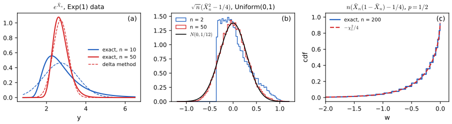
fig_5_s4. Download: PDF · SVGTheorem 5.15 (the multivariate delta method) pp. 79–80
Suppose \(\sqrt n(Y_n-\mu)\)
(The book assumes that every element of \(\nabla_\mu\) is nonzero; this is not needed, see Filling the gap 5.12.)
Filling the gap 5.12: proof of the multivariate delta method p. 80
The proof needs only differentiability of \(g\) at \(\mu\). The limit is nondegenerate exactly when \(\nabla_\mu^\T\Sigma\nabla_\mu\)
Proof
Differentiability at \(\mu\) means \(g(y)-g(\mu)\)
\(V_n\) is bounded in probability (multivariate (T)), so \(Y_n\cP\mu\) and \(r(Y_n)\cP0\) as in the univariate proof, and the second term tends to 0 in probability by (L1). The first term is a continuous (linear) function of \(V_n\), so it converges in distribution to \(\nabla_\mu^\T V\) with \(V\sim N(0,\Sigma)\), which is \(N(0,\nabla_\mu^\T\Sigma\nabla_\mu)\). Slutsky's theorem 5.5(c) adds the two. Nothing required the components of \(\nabla_\mu\) to be nonzero: for \(g(y_1,y_2)=y_1\) the theorem correctly returns the marginal limit \(N(0,\sigma_{11})\). ∎
Example 5.16. p. 80 For iid pairs \((X_{1i},X_{2i})\) with mean \((\mu_1,\mu_2)\) and covariance \(\Sigma=(\sigma_{jk})\), let \(Y_n=\overline X_1\overline X_2\), so \(g(s_1,s_2)=s_1s_2\) and \(\nabla g(s)=(s_2,s_1)^\T\). Then
\[ \sqrt n\,(\overline X_1\overline X_2-\mu_1\mu_2)\cd N\big(0,\ \mu_2^2\sigma_{11}+2\mu_1\mu_2\sigma_{12}+\mu_1^2\sigma_{22}\big). \]For \(X=(E_1,E_1+E_2)\) with \(E_1,E_2\) independent Exp(1), \(\mu=(1,2)\), \(\Sigma=\begin{pmatrix}1&1\\1&2\end{pmatrix}\), the variance is \(4+4+2=10\); Monte Carlo gives a standard deviation of \(\sqrt n(\overline X_1\overline X_2-2)\) of 3.19 at \(n=500\) against \(\sqrt{10}=3.16\) (Figure 5.S5(b)).
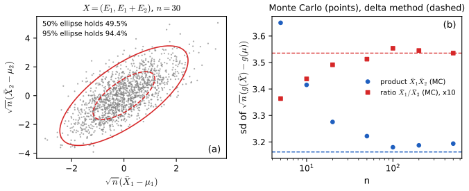
fig_5_s5. Download: PDF · SVG5.6 Bibliographic Remarks
p. 80 The book points to Grimmett and Stirzaker (1982), Karr (1993) and Billingsley (1979) for convergence in probability theory, and to van der Vaart and Wellner (1996) and van der Vaart (1998) for its modern statistical use. For the proofs filled in here, Billingsley (1995, Sections 6, 25 and 27), Durrett (2019, Chapters 2 and 3) and Feller (1971, Chapter XVI) are the standard sources; van der Vaart (1998, Chapters 2 and 3) treats Slutsky's theorem, the continuous mapping theorem and the delta method in the form used throughout statistics.
5.7 Appendix
5.7.1 Almost Sure and L1 Convergence
Definition (almost-sure and \(L^1\) convergence) p. 81
\(X_n\) converges almost surely to \(X\), written \(X_n\cas X\), if \(\P(\{\omega:X_n(\omega)\to X(\omega)\})\)
Theorem 5.17 p. 81
(a) \(X_n\cas X\) implies \(X_n\cP X\). (b) \(X_n\cqm X\) implies \(X_n\cL X\). (c) \(X_n\cL X\) implies \(X_n\cP X\).
Filling the gap 5.13: proof of Theorem 5.17, the Borel–Cantelli lemmas, and the missing arrows p. 81
(i) \(X_n\cas X\) iff \(\P(\sup_{m\ge n}|X_m-X|>\eps)\)
Proof
(i). Let \(A_n(\eps)\)
Theorem 5.17(a) follows: \(\P(|X_n-X|>\eps)\)
(ii). \(\P(\text{infinitely many }A_m)\)
(iii). By independence and \(1-x\le e^{-x}\), for \(N\ge n\), \(\P(\bigcap_{m=n}^NA_m^c)\)
(iv). Choose \(n_1<n_2<\dots\) with \(\P(|X_{n_k}-X|>2^{-k})\)
The missing arrows. Probability does not imply almost surely, and quadratic mean does not imply almost surely: independent \(\I(U_n<1/n)\) converge in quadratic mean but, by (iii), not almost surely. Almost surely does not imply \(L^1\): \(n^2\I(U<1/n)\). \(L^1\) does not imply quadratic mean: \(n^{3/4}\I(U<1/n)\). With \(b=2\) instead, independent spikes \(\I(U_n<n^{-2})\) do converge almost surely, by (ii); exactly, \(\P(\text{a spike at some }m\ge n)\)
The weak law says \(\Xb\cP\mu\); the strong law upgrades this to almost-sure convergence.
Theorem 5.18 (the strong law of large numbers) p. 81
Let \(X_1,X_2,\dots\) be iid. If \(\E|X_1|<\infty\), then \(\Xb\cas\mu=\E X_1\).
(The book writes "if \(\mu=\E|X_1|<\infty\) then \(\Xb\cas\mu\)", which names the wrong limit: see Notes on the book.)
Filling the gap 5.14: proof of the strong law (Etemadi 1981) p. 81
The book states the strong law without proof. Etemadi's proof needs only pairwise independence and a finite mean, and uses nothing beyond Chebyshev's inequality and the first Borel–Cantelli lemma.
Proof
Reduction. Write \(X_i=X_i^+-X_i^-\); both parts are iid, nonnegative and integrable, and if the averages of each converge almost surely, so does their difference. So assume \(X_i\ge0\), \(\mu=\E X_1<\infty\). Let \(S_n=\sum_{i\le n}X_i\).
Step 1 (truncation). Let \(Y_i=X_i\I(X_i\le i)\) and \(T_n=\sum_{i\le n}Y_i\). Then \(\sum_i\P(Y_i\ne X_i)\)
Step 2 (the means). \(\E Y_i\)
Step 3 (a geometric subsequence). Fix \(\alpha>1\) and let \(k_m=\lfloor\alpha^m\rfloor\). By Chebyshev and independence,
\[ \sum_m\P\big(|T_{k_m}-\E T_{k_m}|>\eps k_m\big)\le\frac1{\eps^2}\sum_m\frac{1}{k_m^2}\sum_{i\le k_m}\E Y_i^2=\frac1{\eps^2}\sum_i\E Y_i^2\sum_{m:\,k_m\ge i}\frac1{k_m^2}. \]Since \(k_m\ge\alpha^m/2\), the inner sum is at most \(4\sum_{m:\alpha^m\ge i}\alpha^{-2m}\)
Step 4 (filling in). \(T_n\) is nondecreasing because \(Y_i\ge0\). For \(k_m\le n\le k_{m+1}\), \(T_{k_m}/k_{m+1}\)
The converse. If \(\E|X_1|=\infty\), then \(\sum_n\P(|X_1|>n)=\infty\), so by the second Borel–Cantelli lemma \(|X_n|>n\) infinitely often, and \(X_n/n\)
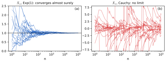
fig_5_s6. Download: PDF · SVGDefinition (asymptotic uniform integrability) p. 81
\(X_n\) is asymptotically uniformly integrable if \(\lim_{M\to\infty}\limsup_{n\to\infty}\E\big(|X_n|\I(|X_n|>M)\big)\)
Theorem 5.19 p. 81
If \(X_n\cP b\) and \(X_n\) is asymptotically uniformly integrable, then \(\E X_n\to b\).
Filling the gap 5.15: proof of Theorem 5.19 p. 81
The book states the result without proof. Uniform integrability is exactly what the warning example lacks: for \(\P(X_n=n^2)=1/n\), \(\E|X_n|\I(|X_n|>M)=n\) as soon as \(n^2>M\).
Proof
Let \(\eps>0\) and choose \(M>|b|+1\) with \(\limsup_n\E|X_n|\I(|X_n|>M)\)
The middle term is at most \(\eps\) in absolute value for large \(n\). Since \(M>|b|+1\), \(\{|X_n|>M\}\subset\{|X_n-b|>1\}\), so the last term tends to 0. For the first, fix \(\delta\in(0,1)\): on \(\{|X_n-b|\le\delta\}\) the integrand is at most \(\delta\), and elsewhere (with \(|X_n|\le M\)) at most \(M+|b|\), so it is at most \(\delta\)
A convenient sufficient condition: \(\sup_n\E|X_n|^{1+\eta}\)
5.7.2 Proof of the Central Limit Theorem
pp. 81–82 The book's proof uses moment generating functions \(\psi_X(t)=\E e^{tX}\), assumed finite in a neighbourhood of 0, and the following lemma.
Lemma 5.20 (convergence of moment generating functions) p. 81
Let \(Z_1,Z_2,\dots\) have mgfs \(\psi_n\) and \(Z\) have mgf \(\psi\). If \(\psi_n(t)\to\psi(t)\) for all \(t\) in an open interval around 0, then \(Z_n\cd Z\).
With \(Y_i=(X_i-\mu)/\sigma\) and \(\psi\) the mgf of \(Y_1\), the mgf of \(Z_n=n^{-1/2}\sum_iY_i\) is \(\xi_n(t)=\psi(t/\sqrt n)^n\). Since \(\psi(0)=1\), \(\psi'(0)=\E Y_1=0\) and \(\psi''(0)=\E Y_1^2=1\),
\[ \xi_n(t)=\Big[1+\frac{t^2}{2n}+\frac{t^3}{3!\,n^{3/2}}\psi'''(0)+\cdots\Big]^n\to e^{t^2/2}, \]the mgf of \(N(0,1)\), and Lemma 5.20 concludes.
Filling the gap 5.16: the book's proof made rigorous, and a proof of Lemma 5.20 pp. 81–82
Three steps are left implicit: (a) that \(\psi\) can be differentiated at 0 with \(\psi^{(k)}(0)=\E Y^k\) and the dots controlled; (b) the limit \((1+a_n/n)^n\to e^a\) when \(a_n\to a\); (c) Lemma 5.20 itself.
Proof
(a). Suppose \(\psi(t)<\infty\) for \(|t|<t_0\). For \(|t|\le s<t_0\) and any \(k\), \(|y|^ke^{ty}\)
No infinite series is needed.
(b). For \(|x|\le\tfrac12\), \(|\log(1+x)-x|\le x^2\). If \(a_n\to a\), then for large \(n\), \(|a_n/n|\le\tfrac12\) and \(|n\log(1+a_n/n)-a_n|\)
(c) Lemma 5.20. Let \(\psi_n\to\psi\) on \((-t_0,t_0)\) and fix \(0<s<t_0\). Tightness: by Markov's inequality, \(\P(|Z_n|>M)\)
The moment generating function proof thus needs more than a finite variance (the mgf must exist) and leans on the uniqueness theorem. Lindeberg's argument in Filling the gap 5.7 avoids both. The standard textbook route uses characteristic functions \(\E e^{itX}\), which always exist, and Lévy's continuity theorem in place of Lemma 5.20.
Notes on the book
Seven places where the text of Chapter 5 needs a correction or a qualification. Four are in the author's own errata lists on the book's website; three are not, and the evidence for each is given.
Page 71: the second example should read \(X_n\sim N(0,1/n)\)
The text says "consider \(X_1,X_2,\dots\) where \(X_i\sim N(0,1/n)\)". The variance must depend on the index of the variable, not on a free \(n\): the sequence meant is \(X_n\sim N(0,1/n)\), as the next sentence ("\(X_n\) is very concentrated around 0 for large \(n\)") and Example 5.3 confirm. (Not in the author's errata lists.)
Page 73, Example 5.3: \(F(1/2)\) should be \(F(0)\)
"\(F_n(0)=1/2\ne F(1/2)=1\)" should compare \(F_n(0)\) with \(F(0)=1\). Listed in the author's errata.
Page 80, Theorem 5.15: the assumption that every element of \(\nabla_\mu\) is nonzero is not needed
The conclusion holds whenever \(g\) is differentiable at \(\mu\), with a degenerate normal limit when \(\nabla_\mu^\T\Sigma\nabla_\mu\)
Page 81, top: \(X_n(s)\) and \(X(s)\) should be \(X_n(\omega)\) and \(X(\omega)\)
The sample point is \(\omega\) throughout the book. Listed in the author's errata.
Page 81, Theorem 5.18: the limit of \(\Xb\) is \(\E X_1\), not \(\E|X_1|\)
The theorem reads "If \(\mu=\E|X_1|<\infty\) then \(\Xb\cas\mu\)". The condition is right (a finite first absolute moment), but the limit is \(\E X_1\), which differs from \(\E|X_1|\) unless \(X_1\ge0\). For \(X_i\sim N(-1,1)\), \(\Xb\to-1\) almost surely while \(\E|X_1|\)
Page 82, Exercise 5.1(b): "part (e)" should be "part (d)"; page 83, Exercise 5.4 should start at \(n=2\); Exercise 5.6 should ask about 72 inches
All three are listed in the author's errata. In Exercise 5.4 at \(n=1\) the two values \(1/n\) and \(n\) coincide and the stated probabilities \(1-1/n^2=0\) and \(1/n^2=1\) clash. In Exercise 5.6 the probability that an average is at least the population mean is \(\tfrac12\) by any symmetric approximation, which is why the corrected question asks about 72 inches (both versions are solved below).
Page 78, (5.4) and Example 5.7: valid but far from sharp
Two bounds in the chapter are correct but very conservative, which matters when they are used for sample-size calculations. The constant \(33/4\) in (5.4) can be replaced by 0.4748 (Filling the gap 5.9); Chebyshev's \(n=84\) in Example 5.7 compares with an exact \(n\ge29\) (Filling the gap 5.6). Also, Lemma 5.20 and the appendix proof of the CLT assume a finite moment generating function, which Theorem 5.8 does not; the theorem itself is true under a finite variance alone (Filling the gap 5.7). (Not in the author's errata lists; these are qualifications rather than errors.)
Exercises
All 16 exercises of Chapter 5 (Wasserman 2004, pp. 82–84), restated in my own words, with complete solutions (hidden).
Exercise 5.1. \(X_1,\dots,X_n\) are iid with finite mean \(\mu\) and variance \(\sigma^2\). (a) Show \(\E S_n^2=\sigma^2\). (b) Show \(S_n^2\cP\sigma^2\), by writing \(S_n^2\)
\({}=c_n\,n^{-1}\sum_iX_i^2-d_n\Xb^2\) with \(c_n,d_n\to1\). Solution
(a) \(\sum_i(X_i-\Xb)^2\)
\({}=\sum_i(X_i-\mu)^2-n(\Xb-\mu)^2\) (expand \(X_i-\Xb=(X_i-\mu)-(\Xb-\mu)\) and use \(\sum_i(X_i-\mu)=n(\Xb-\mu)\)). Taking expectations, \(\E\sum_i(X_i-\Xb)^2\) \({}=n\sigma^2-n\cdot\sigma^2/n\) \({}=(n-1)\sigma^2\), so \(\E S_n^2=\sigma^2\). (b) \(\sum_i(X_i-\Xb)^2\)
\({}=\sum_iX_i^2-n\Xb^2\), so \(S_n^2\) \({}=\frac n{n-1}\cdot\frac1n\sum_iX_i^2-\frac n{n-1}\Xb^2\): \(c_n=d_n=n/(n-1)\to1\). The \(X_i^2\) are iid with finite mean \(\sigma^2+\mu^2\), so by the weak law (Filling the gap 5.5, which needs only the mean) \(n^{-1}\sum X_i^2\) \({}\cP\sigma^2+\mu^2\); and \(\Xb\cP\mu\), so \(\Xb^2\cP\mu^2\) by Theorem 5.5(d) (the book's hint says part (e); part (d) is meant, as the author's errata note) or (f). Constants converging to 1 are trivially convergent in probability, and Theorem 5.5(a), (d) give \(S_n^2\) \(\cP1\cdot(\sigma^2+\mu^2)-1\cdot\mu^2\) \({}=\sigma^2\). Exercise 5.2. Show that \(X_n\cqm b\) if and only if \(\E X_n\to b\) and \(\V X_n\to0\).
Solution
For a random variable with finite variance and a constant \(b\), \(\E(X_n-b)^2\)
\({}=\V(X_n)+(\E X_n-b)^2\) (bias–variance decomposition: expand around \(\E X_n\); the cross term has mean 0). Both terms are nonnegative, so the sum tends to 0 if and only if each does. (If \(\V X_n=\infty\) for infinitely many \(n\), neither side holds.) Exercise 5.3. If \(X_1,\dots,X_n\) are iid with mean \(\mu\) and finite variance, show \(\Xb\cqm\mu\).
Solution
\(\E\Xb=\mu\) and \(\V\Xb=\sigma^2/n\to0\); by Exercise 5.2, \(\Xb\cqm\mu\). Directly, \(\E(\Xb-\mu)^2=\sigma^2/n\).
Exercise 5.4. For \(n\ge2\) let \(\P(X_n=1/n)=1-1/n^2\) and \(\P(X_n=n)=1/n^2\). Does \(X_n\) converge in probability? In quadratic mean?
Solution
In probability, yes, to 0. For \(\eps>0\) and \(n>1/\eps\), \(|X_n|>\eps\) only when \(X_n=n\), so \(\P(|X_n|>\eps)=1/n^2\to0\).
In quadratic mean, no. \(\E X_n^2\)
\({}=\frac{1}{n^2}(1-\frac1{n^2})\) \({}+n^2\cdot\frac1{n^2}\) \({}=1+\frac1{n^2}-\frac1{n^4}\) \(\to1\ne0\). By Theorem 5.4(a) a quadratic-mean limit would have to be the probability limit 0, so there is no quadratic-mean limit at all. (Also \(\E X_n\to0\) but \(\V X_n\to1\), in line with Exercise 5.2. It does converge almost surely, by Borel–Cantelli, since \(\sum1/n^2<\infty\), whatever the joint law.) Exercise 5.5. For \(X_1,\dots,X_n\) iid Bernoulli\((p)\), prove that \(n^{-1}\sum_iX_i^2\cP p\) and \(n^{-1}\sum_iX_i^2\cqm p\).
Solution
A 0/1 variable satisfies \(X_i^2=X_i\), so \(n^{-1}\sum X_i^2=\Xb\), with mean \(p\) and variance \(p(1-p)/n\to0\). So \(\Xb\cqm p\) (Exercise 5.2), hence \(\Xb\cP p\) (Theorem 5.4(a)).
Exercise 5.6. Men's heights have mean 68 inches and standard deviation 2.6 inches. For 100 men drawn at random, approximate the probability that the average height is at least 68 inches (in the corrected version: at least 72 inches).
Solution
By the CLT, \(\Xb\approx N(68,2.6^2/100)\), standard deviation 0.26. (i) As printed: \(\P(\Xb\ge68)\)
\({}\approx\P(Z\ge0)\) \({}=\tfrac12\). (ii) Corrected: \(\P(\Xb\ge72)\) \({}\approx\P(Z\ge4/0.26)\) \({}=\P(Z\ge15.4)\) \(\approx10^{-53}\), effectively zero. The normal approximation is not trustworthy that far in the tail (its relative error there is uncontrolled; (5.4) only bounds the absolute error), but any reasonable model gives a negligible probability: by Chebyshev it is at most \(0.26^2/4^2=0.004\). Exercise 5.7. Let \(X_n\sim\) Poisson\((1/n)\). (a) Show \(X_n\cP0\). (b) Show \(Y_n=nX_n\cP0\).
Solution
(a) \(X_n\) takes values in \(\{0,1,2,\dots\}\), so for \(0<\eps<1\), \(\P(|X_n|>\eps)\)
\({}=\P(X_n\ge1)\) \({}=1-e^{-1/n}\) \(\le1/n\to0\). (b) \(\{|nX_n|>\eps\}=\{X_n\ge1\}\) for every \(\eps\in(0,n)\), with the same probability \(1-e^{-1/n}\to0\). Note that \(\E Y_n=1\) for every \(n\): another sequence converging in probability whose means do not converge to the limit. Exercise 5.8. A program has 100 pages; the numbers of errors \(X_i\) on the pages are independent Poisson(1). Approximate \(\P(Y<90)\) for the total \(Y=\sum_iX_i\).
Solution
\(\E Y=100\), \(\V Y=100\). CLT: \(\P(Y<90)\)
\({}\approx\Phi((90-100)/10)\) \({}=\Phi(-1)\) \({}=0.1587\). Since \(Y\) is integer-valued, \(\P(Y<90)=\P(Y\le89)\), and the continuity correction gives \(\Phi((89.5-100)/10)\) \({}=\Phi(-1.05)\) \({}=0.1469\). Exactly, \(Y\sim\) Poisson(100) and \(\P(Y\le89)=0.1463\): the corrected approximation is accurate to 0.0006, the uncorrected one is off by 0.012. Exercise 5.9. \(\P(X=1)=\P(X=-1)=\tfrac12\); \(X_n=X\) with probability \(1-1/n\) and \(X_n=e^n\) with probability \(1/n\). Does \(X_n\to X\) in probability? In distribution? Does \(\E(X-X_n)^2\to0\)?
Solution
Take the choice between \(X\) and \(e^n\) independent of \(X\). In probability: yes. \(\P(|X_n-X|>\eps)\)
\({}\le\P(X_n\ne X)\) \({}=1/n\to0\). In distribution: yes, by Theorem 5.4(b) (directly: \(F_n(t)\) \({}=(1-1/n)F(t)+\frac1n\I(t\ge e^n)\) \({}\to F(t)\) for every \(t\)). In quadratic mean: no. \(\E(X-X_n)^2\) \({}=\frac1n\E(X-e^n)^2\) \({}=\frac1n(\E X^2-2e^n\E X+e^{2n})\) \({}=\frac{1+e^{2n}}{n}\) \({}\to\infty\). Exercise 5.10. For \(Z\sim N(0,1)\), \(t>0\) and \(k>0\), show \(\P(|Z|>t)\le\E|Z|^k/t^k\), and compare with Mill's inequality.
Solution
Markov's inequality for \(|Z|^k\ge0\): \(\P(|Z|>t)\)
\({}=\P(|Z|^k>t^k)\) \({}\le\E|Z|^k/t^k\). Here \(\E|Z|^k\) \({}=2^{k/2}\Gamma((k+1)/2)/\sqrt\pi\). Mill's inequality (Chapter 4) gives \(\P(|Z|>t)\) \({}\le\sqrt{2/\pi}\,e^{-t^2/2}/t\). For every fixed \(k\) the moment bound decays only like \(t^{-k}\), while Mill's decays like \(e^{-t^2/2}\), so Mill's wins for large \(t\). Optimising \(k\) helps (the best \(k\) is about \(t^2\)) but not enough: \(t\) exact \(\P(|Z|>t)\) Mill's Chebyshev (\(k=2\)) best \(k\) moment bound at best \(k\) 2 0.0455 0.0540 0.25 4 0.1875 3 0.00270 0.00295 0.111 9 0.0156 4 6.33e-5 6.69e-5 0.0625 16 4.72e-4 Mill's bound is within 20% of the truth; the best moment bound is 4 to 7 times too large.
Exercise 5.11. \(X_n\sim N(0,1/n)\) and \(X\) has cdf \(F(x)=\I(x\ge0)\). Does \(X_n\to X\) in probability? In distribution?
Solution
\(X\) is the point mass at 0. In probability: yes: \(\P(|X_n-0|>\eps)\)
\({}=2\Phi(-\eps\sqrt n)\) \(\to0\) (or Chebyshev, \(\le1/(n\eps^2)\)). In distribution: yes, either by Theorem 5.4(b) or directly as in Example 5.3: \(F_n(x)=\Phi(\sqrt nx)\to F(x)\) for \(x\ne0\), and 0 is the only discontinuity of \(F\). Exercise 5.12. \(X,X_1,X_2,\dots\) take positive integer values. Show that \(X_n\cd X\) iff \(\P(X_n=k)\to\P(X=k)\) for every integer \(k\).
Solution
The cdf \(F\) of \(X\) is a step function, continuous at every non-integer, and \(F_n(k+\tfrac12)=\P(X_n\le k)\).
\((\Rightarrow)\) \(k\pm\tfrac12\) are continuity points of \(F\), so \(\P(X_n=k)\)
\({}=F_n(k+\tfrac12)-F_n(k-\tfrac12)\) \({}\to F(k+\tfrac12)-F(k-\tfrac12)\) \({}=\P(X=k)\). \((\Leftarrow)\) For \(t\) not an integer, \(F_n(t)=\sum_{k\le t}\P(X_n=k)\), a finite sum over \(k=1,\dots,\lfloor t\rfloor\) (the values are positive integers), so it converges to \(\sum_{k\le t}\P(X=k)=F(t)\). Every continuity point of \(F\) that is an integer \(k\) (a value of probability 0) is handled the same way, since \(F_n(k)=F_n(k+\tfrac12)\) for integer-valued variables. The finiteness of the sum is what makes the exchange of limit and sum legitimate.
Exercise 5.13. \(Z_1,Z_2,\dots\) are iid with density \(f\), \(\P(Z_i>0)=1\), and \(\lambda\)
\({}=\lim_{x\downarrow0}f(x)\) \({}>0\). Show that \(X_n=n\min\{Z_1,\dots,Z_n\}\cd\) Exponential with mean \(1/\lambda\). Solution
Let \(F\) be the cdf of \(Z_1\); \(F(0)=0\). For \(x>0\), by independence,
\[ \P(X_n>x)=\P(Z_1>x/n)^n=\big(1-F(x/n)\big)^n. \]By the mean value theorem for integrals and \(f(u)\to\lambda\) as \(u\downarrow0\), \(F(x/n)\)
\({}=\int_0^{x/n}f(u)\,\d u\) \({}=\frac xn(\lambda+o(1))\). So \(\P(X_n>x)=(1-a_n/n)^n\) with \(a_n\) \({}=x(\lambda+o(1))\) \({}\to\lambda x\), and by the limit in Filling the gap 5.16(b), \(\P(X_n>x)\to e^{-\lambda x}\). For \(x\le0\), \(\P(X_n\le x)=0\). The limit cdf \(1-e^{-\lambda x}\) (for \(x>0\)) is continuous, the Exponential law with mean \(1/\lambda\). (A simulation with half-normal \(Z_i\), \(\lambda=\sqrt{2/\pi}\), and \(n=200\) agrees with the limit to within Monte Carlo error.) Exercise 5.14. \(X_1,\dots,X_n\sim\) Uniform(0,1) and \(Y_n=\Xb^2\). Find the limiting distribution of \(Y_n\).
Solution
\(Y_n\cP\tfrac14\) (weak law and continuous mapping), so the "limiting distribution" of \(Y_n\) itself is the point mass at \(\tfrac14\). The informative statement is the delta method: \(\mu=\tfrac12\), \(\sigma^2=\tfrac1{12}\), \(g(s)=s^2\), \(g'(\tfrac12)=1\), so
\[ \sqrt n\,\big(\Xb^2-\tfrac14\big)\cd N\big(0,\tfrac1{12}\big),\qquad\text{i.e. }Y_n\approx N\big(\tfrac14,\tfrac1{12n}\big). \]Figure 5.S4(b) shows the simulated law at \(n=2\) (skewed, bounded below by \(-\sqrt2/4\)) and at \(n=50\) (close to the limit).
Exercise 5.15. For iid pairs \((X_{1i},X_{2i})\) with mean \((\mu_1,\mu_2)\), \(\mu_2\ne0\), and covariance \(\Sigma\), find the limiting distribution of \(Y_n\)
\({}=\overline X_1/\overline X_2\). Solution
\(g(s_1,s_2)=s_1/s_2\) is differentiable at \(\mu\) with \(\nabla g(\mu)\)
\[ \sqrt n\Big(\frac{\overline X_1}{\overline X_2}-\frac{\mu_1}{\mu_2}\Big)\cd N\Big(0,\ \frac{\sigma_{11}}{\mu_2^2}-\frac{2\mu_1\sigma_{12}}{\mu_2^3}+\frac{\mu_1^2\sigma_{22}}{\mu_2^4}\Big). \]\({}=(1/\mu_2,\,-\mu_1/\mu_2^2)^\T\). By the multivariate CLT and Theorem 5.15, (\(\overline X_2\ne0\) with probability tending to 1, so \(Y_n\) is defined on an event whose probability tends to 1, which is enough.) For \(X=(E_1,E_1+E_2)\): \(1/4-2\cdot1/8+2/16=1/8\), and Monte Carlo gives a standard deviation of \(\sqrt n(Y_n-\tfrac12)\) of 0.354 at \(n=500\) against \(\sqrt{1/8}=0.354\) (Figure 5.S5(b)).
Exercise 5.16. Construct \(X_n\cd X\) and \(Y_n\cd Y\) such that \(X_n+Y_n\) does not converge in distribution to \(X+Y\).
Solution
Let \(X,Y\) be independent \(N(0,1)\), and set \(X_n=X\), \(Y_n=-X\) for every \(n\). Then \(X_n\cd X\) trivially, and \(Y_n\cd Y\) because \(-X\sim N(0,1)\), the law of \(Y\). But \(X_n+Y_n=0\) for every \(n\), while \(X+Y\sim N(0,2)\). The marginal limits do not determine the limit of the sum; one needs the joint law, which is why Slutsky's theorem asks one of the limits to be a constant (a constant limit pins down the joint limit: \((X_n,Y_n)\cd(X,c)\)).
Demonstrations for this chapter
Each demonstration runs in the browser and links back to these notes. The ▶ Demo boxes above open them already set to the case under discussion.
| Demonstration | What you can see | Sections and results |
|---|---|---|
| Modes of convergence and their counterexamples | Spikes \(n^a\I(U_n<n^{-b})\) with one or independent uniforms, \(N(0,1/n)\) and \(X_n=-X\): 25 sample paths, exact tail probabilities and moments against \(n\), Monte Carlo over 2000 paths of the probability of a later exceedance, and a verdict for each mode. Presets: 1 the book's example; 2 independent spikes; 3 Borel–Cantelli; 4 the warning example; 5 \(X_n=-X\); 6 Example 5.3. | 5.2, 5.7.1; Theorem 5.4, Theorem 5.17, Filling the gaps 5.2, 5.13 |
| The exact Berry–Esseen error | For gamma, Bernoulli and Poisson observations, the exact error \(\P(Z_n\le z)-\Phi(z)\) as a function of \(z\) with its Edgeworth approximation, and the exact distance \(d_n\) against \(n\) with the bound (5.4) for \(C=33/4\) and \(C=0.4748\). Presets: 1 exponential; 2 Bernoulli(1/2); 3 rare events; 4 Gamma(1/4); 5 one Poisson(5). | 5.4; Theorem 5.8, Theorem 5.11, Filling the gap 5.9 |
| The delta method | \(g(\Xb)\) for exponential, Bernoulli and Poisson samples and seven transformations: \(g\) with its tangent over the law of \(\Xb\), the exact cdf of \(g(\Xb)\) against the delta method (or the \(\chi^2_1\) limit when \(g'(\mu)=0\)), exact means and standard deviations, and the Kolmogorov distance against \(n\). Presets: 1 Example 5.14; 2 square root for Poisson; 3 log; 4 reciprocal; 5 \(g'(\mu)=0\); 6 arcsine. | 5.5; Theorem 5.13, Filling the gap 5.11 |
Related demonstrations: the first-year central limit theorem demo (simulated averages from four populations), and the variance-stabilisation demo of Statistical Methods for Modern Biology. The Python code that produces every figure of this page is code/ch05_convergence.py (see the code index).
References
- Wasserman, L. (2004). All of Statistics: A Concise Course in Statistical Inference. Springer, New York. Chapter 5, pp. 71–84. www.stat.cmu.edu/~larry/all-of-statistics.
- Berry, A. C. (1941). The accuracy of the Gaussian approximation to the sum of independent variates. Transactions of the American Mathematical Society, 49(1), 122–136.
- Billingsley, P. (1995). Probability and Measure, 3rd edition. Wiley, New York.
- Cramér, H. and Wold, H. (1936). Some theorems on distribution functions. Journal of the London Mathematical Society, 11(4), 290–294.
- Curtiss, J. H. (1942). A note on the theory of moment generating functions. The Annals of Mathematical Statistics, 13(4), 430–433.
- Durrett, R. (2019). Probability: Theory and Examples, 5th edition. Cambridge University Press, Cambridge.
- Esseen, C.-G. (1942). On the Liapounoff limit of error in the theory of probability. Arkiv för Matematik, Astronomi och Fysik, 28A(9), 1–19.
- Esseen, C.-G. (1945). Fourier analysis of distribution functions. A mathematical study of the Laplace–Gaussian law. Acta Mathematica, 77, 1–125.
- Esseen, C.-G. (1956). A moment inequality with an application to the central limit theorem. Skandinavisk Aktuarietidskrift, 39, 160–170.
- Etemadi, N. (1981). An elementary proof of the strong law of large numbers. Zeitschrift für Wahrscheinlichkeitstheorie und verwandte Gebiete, 55(1), 119–122.
- Feller, W. (1971). An Introduction to Probability Theory and Its Applications, Volume II, 2nd edition. Wiley, New York.
- Grimmett, G. and Stirzaker, D. (1982). Probability and Random Processes. Oxford University Press, Oxford.
- Lindeberg, J. W. (1922). Eine neue Herleitung des Exponentialgesetzes in der Wahrscheinlichkeitsrechnung. Mathematische Zeitschrift, 15, 211–225.
- Mann, H. B. and Wald, A. (1943). On stochastic limit and order relationships. The Annals of Mathematical Statistics, 14(3), 217–226.
- Shevtsova, I. G. (2011). On the absolute constants in the Berry–Esseen type inequalities for identically distributed summands. Preprint, arXiv.
- Slutsky, E. (1925). Über stochastische Asymptoten und Grenzwerte. Metron, 5(3), 3–89.
- van der Vaart, A. W. (1998). Asymptotic Statistics. Cambridge University Press, Cambridge.
- van der Vaart, A. W. and Wellner, J. A. (1996). Weak Convergence and Empirical Processes. Springer, New York.
The numerical statements in the text (the exact probabilities of Examples 5.7 and 5.9 and Exercises 5.6–5.10, the moments and tail probabilities of the counterexamples, the Borel–Cantelli product, the Berry–Esseen distances and constants, the Edgeworth corrections, the rate for smooth test functions, the delta-method means and variances of Examples 5.14 and 5.16 and Exercises 5.14–5.15, and the corrections listed in the notes on the book) were confirmed numerically.