Support Vector Machines and Flexible Discriminants
Two families of classifiers that start from a linear rule and make it flexible. The support vector machine starts from the maximum-margin hyperplane of Chapter 4, lets points violate the margin at a price, and moves to a huge feature space through a kernel; seen from the other side it is a penalised fit with the hinge loss, whose minimiser estimates the Bayes classifier itself, and whose whole solution path in the cost parameter is piecewise linear. Flexible, penalised and mixture discriminant analysis start from LDA: LDA turns out to be a sequence of linear regressions on optimally scored class labels, so replacing the regression by a flexible or penalised one, or replacing each class by a mixture of Gaussians, gives nonlinear and regularised discriminants that keep LDA's low-dimensional views.
Ch. 1 Introduction Ch. 2 Supervised learning Ch. 3 Linear regression Ch. 4 Linear classification Ch. 5 Basis expansions Ch. 6 Kernel smoothing Ch. 7 Model assessment Ch. 8 Inference and averaging Ch. 9 Additive models and trees Ch. 10 Boosting Ch. 11 Neural networks Ch. 12 SVMs Ch. 13 Nearest neighbours Ch. 14 Unsupervised learning Ch. 15 Random forests Ch. 16 Ensembles Ch. 17 Graphical models Ch. 18 High-dimensional problems
How to read these notes
They follow the book. Sections carry the book's numbers (12.2, 12.2.1, ...) and every displayed equation that appears in the book carries the book's own equation number, e.g. \((12.13)\), so you can read these notes next to the book. Equations without a number are steps that the book skips.
Filling the gaps. Wherever the book says that something "can be shown", "is easy to show", leaves it to an exercise, or states a property without proof, an orange Filling the gap box or a proof gives the full argument. Proofs and derivations start hidden: open one with its bar, or use the button below.
Figures and demonstrations. All fifteen figures of the chapter are reproduced from scratch by the Python code (Figure 12.1, a schematic in the book, is drawn from a computed fit), and Tables 12.2–12.4 are recomputed. The ▶ Demo boxes open an interactive demonstration already set to the case being discussed.
Main reference
T. Hastie, R. Tibshirani and J. Friedman, The Elements of Statistical Learning: Data Mining, Inference, and Prediction, 2nd edition, Springer (2009), Chapter 12, pages 417–458 (book website, with the data sets: hastie.su.domains/ElemStatLearn). Section, equation, figure, table and exercise numbers below refer to this book. Further reading is listed in the references.
The explanations, derivations, figures and code are my own; equations are cited by their numbers in the book.
Companion courses
Parts of this chapter also appear in the two companion courses on this site. The overlapping material is:
- Sections 12.2–12.2.1 (maximum margin, soft margin, the dual and the KKT conditions): Bayesian and Probabilistic Machine Learning, Section 7.1, 7.1.1, Result 7.2, Result 7.3 and Result 7.6; the KKT conditions in general: Foundations of Deep Learning, Appendix C.2.
- Section 12.3.1 (kernels, positive semidefiniteness, the Gaussian and sigmoid kernels): Bayesian and Probabilistic Machine Learning, Section 6.2, Result 6.1, Filling the gap 6.3 and 6.5.
- Section 12.3.2 (the hinge loss and its relation to logistic regression): Result 7.8 and Section 7.1.2.
- Section 12.3.4 (the curse of dimensionality): Foundations of Deep Learning, Section 6.1.1.
- Sections 12.3.6–12.3.7 (support vector regression and kernel ridge regression): Section 7.1.4, Result 7.9, and the dual representation of Section 6.1.
- Section 12.3.8 (multiclass SVMs, VC dimension and learning bounds): Section 7.1.3 and Section 7.1.5.
- Section 12.5 (Fisher's discriminant and its relation to least squares): Bayesian and Probabilistic Machine Learning, Sections 4.1.4–4.1.6.
- Section 12.7 (EM for Gaussian mixtures): Section 9.2.2 and the general EM argument of Section 9.4.
Within this course the chapter builds on Section 4.5.2 (optimal separating hyperplanes, Result 4.16), Section 4.3 (LDA and its reduced-rank form, Results 4.6 and 4.7), Section 5.8 (reproducing kernels and the representer theorem) and the mixture data of Section 2.3. New here: the path algorithm with its derivation, population minimisers of the four losses, the exact equivalence of optimal scoring and LDA with the weights (12.55), penalised discriminant analysis as LDA in a penalised metric, MDA's M-step by optimal scoring on blurred responses, and three notes on the book (the intercept is not always unique, Figure 12.7, the radius in Figure 12.9).
The chapter at a glance
- 12.2 The soft-margin classifier (12.8) has the dual (12.13) (Result 12.1); the KKT conditions sort the points into three groups and make the fit depend on the support vectors only (Result 12.2); the leave-one-out error is at most the fraction of support vectors (Result 12.3).
- 12.3.1–12.3.3 Everything depends on the data through inner products, so a kernel replaces the feature map (Result 12.4); the SVM is hinge loss plus a ridge penalty (Result 12.5) whose population minimiser is the Bayes rule \(\sgn(p-\tfrac12)\) (Result 12.6); in an RKHS the solution is a finite kernel expansion (Result 12.7).
- 12.3.5 The multipliers \(\alpha_i(\lambda)\) are piecewise linear in \(\lambda=1/C\), so the whole path can be followed from breakpoint to breakpoint (Result 12.8).
- 12.3.6–12.3.8 The \(\epsilon\)-insensitive regression dual (Result 12.9), kernel ridge regression (Result 12.10) and the margin bound on the VC dimension (Result 12.11).
- 12.5–12.6 LDA is optimal scoring with linear regression: the regression coefficients are the discriminant directions and the fits give the Mahalanobis distances with weights \(1/[r_\ell^2(1-r_\ell^2)]\) (Results 12.12 and 12.13); a penalised regression gives LDA in a penalised metric (Result 12.15).
- 12.7 MDA is fitted by EM whose M-step is a weighted LDA, itself an optimal scoring on a blurred response matrix (Result 12.16).
Notation. Training data \((x_i,y_i)\), \(i=1,\dots,N\), \(x_i\in\R^p\); for the SVM \(y_i\in\{-1,+1\}\), for discriminant analysis \(g_i\in\{1,\dots,K\}\). \(f(x)=x^\T\beta+\beta_0\) (or \(h(x)^\T\beta+\beta_0\)), \(\bK\) is the \(N\times N\) kernel matrix \(K(x_i,x_{i'})\), \([u]_+=\max(u,0)\). \(\bY\) is the \(N\times K\) indicator matrix, \(\Dpi=\bY^\T\bY/N\) the diagonal matrix of class proportions; \(\SW\), \(\SB\), \(\ST=\SW+\SB\) are the within, between and total covariance matrices with divisor \(N\).
Prerequisites. Lagrange duality for convex quadratic programs (Appendix C.2 of the companion course), LDA (Section 4.3), the generalised symmetric eigenproblem, and the EM algorithm.
12.1 Introduction
p. 417 Chapter 4 built the optimal separating hyperplane for two classes that a hyperplane can separate. This chapter first allows the classes to overlap (the support vector classifier), then enlarges the feature space through a kernel (the support vector machine), so that a linear boundary in the enlarged space becomes a curved one in the original space. The second half generalises Fisher's linear discriminant analysis in three directions: flexible discriminant analysis (nonlinear boundaries, built much like the SVM), penalised discriminant analysis (many highly correlated features, as in signals and images) and mixture discriminant analysis (classes that are not one Gaussian blob each).
12.2 The Support Vector Classifier
pp. 417–421 The training data are \((x_1,y_1),\dots,(x_N,y_N)\) with \(x_i\in\R^p\) and \(y_i\in\{-1,1\}\).
See also (companion course): Section 7.1, maximum margin classifiers, and Section 7.1.1, overlapping class distributions.
Definition 12.1 (hyperplane, classifier and margin) p. 418, (12.1)–(12.4)
A hyperplane and the rule it induces are
\[ \{x:\ f(x)=x^\T\beta+\beta_0=0\}, \tag{12.1} \] \[ G(x)=\sgn\big[x^\T\beta+\beta_0\big]. \tag{12.2} \]With \(\|\beta\|=1\), \(f(x)\) is the signed distance from \(x\) to the hyperplane (Result 4.13). If the classes are separable, the hyperplane with the largest margin \(M\) solves
\[ \max_{\beta,\beta_0,\ \|\beta\|=1}M\quad\text{subject to}\quad y_i(x_i^\T\beta+\beta_0)\ge M,\ i=1,\dots,N, \tag{12.3} \]or equivalently
\[ \min_{\beta,\beta_0}\|\beta\|\quad\text{subject to}\quad y_i(x_i^\T\beta+\beta_0)\ge1,\ i=1,\dots,N, \tag{12.4} \]with \(M=1/\|\beta\|\). The band of half-width \(M\) on either side of the hyperplane, \(2M\) wide in all, is the margin.
Filling the gap 12.1: why (12.3) and (12.4) are the same problem p. 418
Derivation
For any \((\beta,\beta_0)\) with \(\beta\ne0\) and any \(c>0\), the pairs \((\beta,\beta_0)\) and \((c\beta,c\beta_0)\) describe the same hyperplane and the same rule. In (12.3) drop the constraint \(\|\beta\|=1\) by dividing: \(y_i(x_i^\T\beta+\beta_0)/\|\beta\|\ge M\) for all \(i\) is the same set of conditions for every rescaling of \((\beta,\beta_0)\). Choose the scale with \(\|\beta\|=1/M\); the constraints become \(y_i(x_i^\T\beta+\beta_0)\ge1\), and maximising \(M=1/\|\beta\|\) is minimising \(\|\beta\|\). Conversely a solution of (12.4), divided by \(\|\beta\|\), solves (12.3) with \(M=1/\|\beta\|\). Minimising \(\|\beta\|\) and \(\tfrac12\|\beta\|^2\) have the same solutions, and the second is a convex quadratic program with linear constraints. Chapter 4 proves this in full (Result 4.15). ∎
When the classes overlap, keep maximising \(M\) but let point \(i\) fall short of its margin by a slack \(\xi_i\ge0\), with a budget \(\sum_i\xi_i\le\) constant. There are two natural ways to write the shortfall:
\[ y_i(x_i^\T\beta+\beta_0)\ \ge\ M-\xi_i, \tag{12.5} \] \[ y_i(x_i^\T\beta+\beta_0)\ \ge\ M(1-\xi_i). \tag{12.6} \]The first measures the overlap in absolute distance, the second in units of the margin. Only the second leads to a convex problem, and it is the standard choice. Under (12.6), point \(i\) is misclassified exactly when \(\xi_i>1\) (its signed distance \(M(1-\xi_i)\) is negative), so a budget \(\sum\xi_i\le K\) bounds the number of training errors by \(K\). Rescaling as in Gap 12.1 gives the usual form
\[ \min\|\beta\|\quad\text{subject to}\quad\begin{cases}y_i(x_i^\T\beta+\beta_0)\ge1-\xi_i\ \ \forall i,\\ \xi_i\ge0,\ \ \textstyle\sum\xi_i\le\text{constant}.\end{cases} \tag{12.7} \]Filling the gap 12.2: why (12.6) is convex and (12.5) is not p. 419
Derivation
(12.6) becomes (12.7). Divide (12.6) by \(M\|\beta\|\) after writing \(\beta=\|\beta\|u\) with \(\|u\|=1\) as in (12.3), or more directly: drop the norm constraint and set \(\|\beta\|=1/M\), so that (12.6) reads \(y_i(x_i^\T\beta+\beta_0)\ge1-\xi_i\). The slacks \(\xi_i\) are unchanged by the rescaling because they are relative to \(M\). The feasible set of (12.7) in \((\beta,\beta_0,\xi)\) is an intersection of half-spaces (each constraint is linear), hence convex, and \(\|\beta\|\) is a convex function: (12.7) is a convex program.
(12.5) does not. In (12.5) the slack is an absolute distance, so after rescaling to \(\|\beta\|=1/M\) the constraint becomes \(y_i(x_i^\T\beta+\beta_0)\ge1-\xi_i\|\beta\|\), which contains the product \(\xi_i\|\beta\|\). Its feasible set is not convex in general. Take \(p=1\), one observation \(x=0\), \(y=1\), and \(\beta_0=0\): the constraint is \(0\ge1-\xi|\beta|\), i.e. \(\xi|\beta|\ge1\). The points \((\beta,\xi)=(1,1)\) and \((-1,1)\) are feasible, their midpoint \((0,1)\) is not. ∎
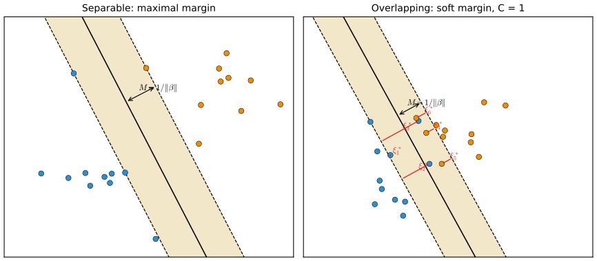
fig_12_1. Reproduces Hastie, Tibshirani and Friedman (2009), Figure 12.1. Download: PDF · SVGBecause the criterion only involves points that are close to or beyond their margins, points deep inside their own class do not shape the boundary. That separates the support vector classifier from LDA, whose boundary depends on all the data through the class means and the pooled covariance; logistic regression is closer to the SVM in this respect (Section 12.3.2).
12.2.1 Computing the Support Vector Classifier
pp. 420–421 For computation the budget in (12.7) is replaced by a cost on the total slack:
\[ \min_{\beta,\beta_0}\ \tfrac12\|\beta\|^2+C\sum_{i=1}^N\xi_i\quad\text{subject to}\quad\xi_i\ge0,\ \ y_i(x_i^\T\beta+\beta_0)\ge1-\xi_i\ \ \forall i, \tag{12.8} \]where the separable case is \(C=\infty\). Each budget in (12.7) corresponds to some \(C\) in (12.8): see Exercise 12.1 and the remark after Result 12.1.
See also (companion courses): Result 7.6, the soft-margin dual; Appendix C.2, inequality constraints and the KKT conditions.
Result 12.1 (the Lagrangian, the Wolfe dual and strong duality) p. 420, (12.9)–(12.13)
With multipliers \(\alpha_i,\mu_i\ge0\) the Lagrange (primal) function of (12.8) is
\[ L_P=\tfrac12\|\beta\|^2+C\sum_{i=1}^N\xi_i-\sum_{i=1}^N\alpha_i\big[y_i(x_i^\T\beta+\beta_0)-(1-\xi_i)\big]-\sum_{i=1}^N\mu_i\xi_i. \tag{12.9} \]Setting its derivatives in \(\beta\), \(\beta_0\) and \(\xi_i\) to zero gives
\[ \beta=\sum_{i=1}^N\alpha_iy_ix_i, \tag{12.10} \] \[ 0=\sum_{i=1}^N\alpha_iy_i, \tag{12.11} \] \[ \alpha_i=C-\mu_i,\quad\forall i, \tag{12.12} \]and substituting back gives the Wolfe dual
\[ L_D=\sum_{i=1}^N\alpha_i-\frac12\sum_{i=1}^N\sum_{i'=1}^N\alpha_i\alpha_{i'}y_iy_{i'}x_i^\T x_{i'}, \tag{12.13} \]to be maximised subject to \(0\le\alpha_i\le C\) and \(\sum_i\alpha_iy_i=0\). For every feasible \((\beta,\beta_0,\xi)\) and every feasible \(\alpha\), \(L_D(\alpha)\) is at most the objective of (12.8) (weak duality), and the maximum of \(L_D\) equals the minimum of (12.8) (strong duality).
Proof
Stationarity. \(L_P\) is a convex quadratic in \((\beta,\beta_0,\xi)\) for fixed multipliers. Its gradient: \(\partial L_P/\partial\beta=\beta-\sum_i\alpha_iy_ix_i\), \(\partial L_P/\partial\beta_0=-\sum_i\alpha_iy_i\), \(\partial L_P/\partial\xi_i=C-\alpha_i-\mu_i\). Setting them to zero gives (12.10)–(12.12).
The dual function. Let \(q(\alpha,\mu)=\inf_{\beta,\beta_0,\xi}L_P\). \(L_P\) is linear in \(\beta_0\) with coefficient \(-\sum\alpha_iy_i\) and linear in each \(\xi_i\) with coefficient \(C-\alpha_i-\mu_i\); unless both coefficients vanish the infimum is \(-\infty\). When they vanish, \(L_P=\tfrac12\|\beta\|^2-\beta^\T\sum_i\alpha_iy_ix_i+\sum_i\alpha_i\), minimised at (12.10), with value \(\sum_i\alpha_i-\tfrac12\|\sum_i\alpha_iy_ix_i\|^2\), which is (12.13). The condition \(\mu_i=C-\alpha_i\ge0\) is \(\alpha_i\le C\).
Weak duality. If \((\beta,\beta_0,\xi)\) is feasible for (12.8) and \(\alpha,\mu\ge0\), the two subtracted sums in (12.9) are nonnegative, so \(L_P\le\tfrac12\|\beta\|^2+C\sum\xi_i\); taking the infimum on the left, \(L_D(\alpha)=q(\alpha,\mu)\le\) the primal objective.
Strong duality. (12.8) is a convex quadratic program with linear constraints and it is feasible (take \(\beta=0\), \(\beta_0=0\), \(\xi_i=1\)); its objective is bounded below by 0, so the minimum is attained. For such programs the KKT conditions are necessary at a minimiser without any further qualification (linear constraints satisfy the Abadie constraint qualification), and the multipliers they provide make \(L_D\) equal to the primal minimum. Numerically, on the mixture data with the radial kernel and \(C=1\) the two optimal values agree to ten digits (86.93328056). ∎
Budget and cost. If \((\beta^*,\beta_0^*,\xi^*)\) solves (12.8) for some \(C\), then it also solves (12.7) with the budget \(\sum\xi_i\le\sum\xi^*_i\): any feasible point of that problem with \(\|\beta\|\lt \|\beta^*\|\) would have a smaller (12.8) objective. So each \(C\) picks out one budget.
In addition to (12.10)–(12.12), the Karush–Kuhn–Tucker conditions include
\[ \alpha_i\big[y_i(x_i^\T\beta+\beta_0)-(1-\xi_i)\big]=0, \tag{12.14} \] \[ \mu_i\xi_i=0, \tag{12.15} \] \[ y_i(x_i^\T\beta+\beta_0)-(1-\xi_i)\ \ge\ 0, \tag{12.16} \]for \(i=1,\dots,N\), and (12.10) gives the solution in terms of the multipliers:
\[ \hat\beta=\sum_{i=1}^N\hat\alpha_iy_ix_i. \tag{12.17} \]Result 12.2 (support vectors: three kinds of points, and which parts of the solution are unique) pp. 420–421, (12.14)–(12.18)
At the solution \(\hat\xi_i=[1-y_i\hat f(x_i)]_+\) and, with \(m_i=y_i\hat f(x_i)\),
- \(m_i>1\) (correct side, outside the margin) \(\Rightarrow\hat\alpha_i=0\);
- \(m_i\lt 1\) (inside the margin or misclassified) \(\Rightarrow\hat\alpha_i=C\);
- \(0\lt \hat\alpha_i\lt C\Rightarrow m_i=1\) (on the margin); points with \(m_i=1\) can have any \(\hat\alpha_i\in[0,C]\).
So \(\hat\beta\) in (12.17) involves only the support vectors (\(\hat\alpha_i>0\)), and any margin point with \(0\lt \hat\alpha_i\lt C\) gives \(\hat\beta_0=y_i-x_i^\T\hat\beta\) (in practice, average them). The classifier is
\[ \hat G(x)=\sgn\big[\hat f(x)\big]=\sgn\big[x^\T\hat\beta+\hat\beta_0\big]. \tag{12.18} \]\(\hat\beta\) is unique. \(\hat\beta_0\) is unique whenever some \(0\lt \hat\alpha_i\lt C\), but not always otherwise.
Proof
For fixed \((\beta,\beta_0)\) the smallest feasible slack is \(\xi_i=[1-y_if(x_i)]_+\), and (12.8) decreases in each \(\xi_i\), so the optimum uses it. If \(m_i>1\), the bracket in (12.14) is \(m_i-1+\xi_i>0\), so \(\alpha_i=0\). If \(m_i\lt 1\), (12.16) forces \(\xi_i\ge1-m_i>0\), (12.15) gives \(\mu_i=0\) and (12.12) gives \(\alpha_i=C\). If \(0\lt \alpha_i\lt C\), (12.12) gives \(\mu_i>0\), (12.15) \(\xi_i=0\), and (12.14) with \(\alpha_i>0\) gives \(m_i=1\). This also identifies \(\alpha_i\) as a (negated) subgradient of the hinge \([1-m]_+\) at \(m_i\), times \(C\).
Uniqueness. Eliminating \(\xi\), (12.8) is
\[ F(\beta,\beta_0)=\tfrac12\|\beta\|^2+C\sum_i[1-y_i(x_i^\T\beta+\beta_0)]_+ \], a convex function. If two pairs are optimal, so is their midpoint, and \(F(\text{midpoint})\le\tfrac12F(1)+\tfrac12F(2)\) with the quadratic term strictly convex: equality forces the two \(\beta\)'s to be equal. For fixed \(\hat\beta\), \(F\) is a convex piecewise-linear function of \(\beta_0\), whose minimisers form a closed interval. A margin point with \(0\lt \hat\alpha_i\lt C\) pins \(\beta_0\) through \(m_i=1\). If every \(\hat\alpha_i\) is 0 or \(C\), the KKT conditions only require \(m_i\ge1\) where \(\hat\alpha_i=0\) and \(m_i\le1\) where \(\hat\alpha_i=C\), a set of linear inequalities in \(\beta_0\) that can define a proper interval. ∎
Note on the book: "uniquely characterize" holds for \(\beta\), not always for \(\beta_0\)
The book says that (12.10)–(12.16) uniquely characterise the solution. They do determine \(\hat\beta\), but \(\hat\beta_0\) can be a whole interval (Burges and Crisp, 1999). This happens on the book's own example: for the linear classifier of Figure 12.2 with \(C=0.01\), no point has \(0\lt \hat\alpha_i\lt C\) (the one point on the margin has \(\hat\alpha_i=0\)), and every \(\beta_0\in[-0.27502,-0.27419]\) is optimal, with the same \(\hat\beta=(-0.1778,\,0.5223)\). The rule \(\hat G\) differs only for points in a thin band. The same remark answers "among these support points, some will lie on the edge of the margin and hence will be characterised by \(0\lt \hat\alpha_i\lt C\)": a margin point can also have \(\hat\alpha_i=0\) or \(\hat\alpha_i=C\).
Maximising the dual is a convex quadratic program in \(N\) variables with box constraints and one equality; the standard solver is sequential minimal optimisation, which updates two multipliers at a time in closed form (see the companion course, Filling the gap 7.3). The course code implements it (svm_smo) and, for the figures, the exact path algorithm of Section 12.3.5. The tuning parameter is the cost \(C\).
12.2.2 Mixture Example (Continued)
pp. 421–422 Figure 12.2 fits the linear support vector classifier to the mixture data of Chapter 2 at two very different costs. With a linear boundary the result hardly depends on \(C\): only the margin changes. Points on the wrong side of their margin are all support vectors, and every misclassified point carries the full weight \(C\), however far away it is.
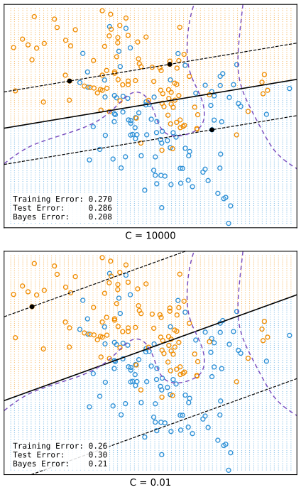
fig_12_2. Reproduces Hastie, Tibshirani and Friedman (2009), Figure 12.2. Download: PDF · SVGThe cost can be chosen by cross-validation (Chapter 7). The book also mentions a bound on the leave-one-out error.
Result 12.3 (the leave-one-out error is at most the fraction of support vectors) p. 421
If the classifier is refitted \(N\) times, each time without one observation, the proportion of left-out points that are misclassified is at most (number of support vectors)/\(N\).
Proof
Let \((\hat\beta,\hat\beta_0,\hat\xi,\hat\alpha,\hat\mu)\) satisfy the KKT conditions for the full data and let \(i\) have \(\hat\alpha_i=0\). Then \(m_i\ge1\), \(\hat\xi_i=0\) and \(\hat\mu_i=C\). Remove observation \(i\): the remaining conditions (12.10)–(12.16) only lose the terms with index \(i\), which contributed nothing to (12.10) and (12.11). So the same \((\hat\beta,\hat\beta_0)\) and the remaining multipliers satisfy the KKT conditions of the reduced problem, and by convexity they solve it. The left-out fit is the full fit, and it classifies \(x_i\) correctly because \(y_i\hat f(x_i)\ge1>0\). Leave-one-out errors can therefore occur only at support vectors. ∎
The bound is loose: 62% and 84% for the two fits of Figure 12.2, against an actual leave-one-out error of 0.280 for \(C=1\), where 63% of the points are support vectors.
12.3 Support Vector Machines and Kernels
pp. 423–424 Like any linear method, the support vector classifier becomes more flexible if the inputs are replaced by basis functions \(h(x)=(h_1(x),\dots,h_M(x))\) (Chapter 5): fit the classifier to \(h(x_i)\) and use \(\hat f(x)=h(x)^\T\hat\beta+\hat\beta_0\), \(\hat G(x)=\sgn\hat f(x)\). The support vector machine lets the dimension \(M\) be very large, even infinite. Two worries follow: the computations, and overfitting, since with enough basis functions the classes become separable. The kernel answers the first; the penalisation view of Section 12.3.2 answers the second.
12.3.1 Computing the SVM for Classification
pp. 423–424 In the enlarged space the dual (12.13) and the solution (12.10) become
\[ L_D=\sum_{i=1}^N\alpha_i-\frac12\sum_{i=1}^N\sum_{i'=1}^N\alpha_i\alpha_{i'}y_iy_{i'}\langle h(x_i),h(x_{i'})\rangle, \tag{12.19} \] \[ f(x)=h(x)^\T\beta+\beta_0=\sum_{i=1}^N\alpha_iy_i\langle h(x),h(x_i)\rangle+\beta_0, \tag{12.20} \]and \(\beta_0\) is found by solving \(y_if(x_i)=1\) for any (or all) \(x_i\) with \(0\lt \alpha_i\lt C\).
Result 12.4 (the kernel trick; the polynomial kernel's features) p. 424, (12.21)–(12.24)
(12.19) and (12.20) involve \(h\) only through the kernel
\[ K(x,x')=\langle h(x),h(x')\rangle, \tag{12.21} \]which must be symmetric and positive semidefinite. Three common choices are
\[ \begin{aligned}&d\text{th-degree polynomial:}&&K(x,x')=(1+\langle x,x'\rangle)^d,\\ &\text{radial basis:}&&K(x,x')=\exp(-\gamma\|x-x'\|^2),\\ &\text{neural network:}&&K(x,x')=\tanh(\kappa_1\langle x,x'\rangle+\kappa_2).\end{aligned} \tag{12.22} \]For two inputs and degree 2,
\[ K(X,X')=(1+X_1X_1'+X_2X_2')^2=1+2X_1X_1'+2X_2X_2'+(X_1X_1')^2+(X_2X_2')^2+2X_1X_1'X_2X_2', \tag{12.23} \]which is \(\langle h(X),h(X')\rangle\) for the \(M=6\) features \(h=(1,\sqrt2X_1,\sqrt2X_2,X_1^2,X_2^2,\sqrt2X_1X_2)\). The solution is
\[ \hat f(x)=\sum_{i=1}^N\hat\alpha_iy_iK(x,x_i)+\hat\beta_0. \tag{12.24} \]In general \((1+\langle x,x'\rangle)^d\) is the inner product of \(\binom{p+d}{d}\) features, all monomials of degree at most \(d\) with fixed multinomial weights. The radial kernel is positive definite with infinitely many features; the tanh kernel is not positive semidefinite in general.
Proof
Inner products only. Replacing \(x\) by \(h(x)\) in Result 12.1 changes nothing in the derivation; \(x_i^\T x_{i'}\) becomes \(\langle h(x_i),h(x_{i'})\rangle\) in (12.13) and \(x^\T\hat\beta=\sum\hat\alpha_iy_ix^\T x_i\) becomes (12.20). The KKT equations used to get \(\beta_0\) involve \(f(x_i)\), again through inner products.
(12.23) and the general degree. Expanding \((1+X_1X_1'+X_2X_2')^2\) gives the six terms shown, and each is the product of a feature at \(X\) and the same feature at \(X'\) (the cross terms carry the factor 2, hence the \(\sqrt2\)'s). For general \(p\) and \(d\), write \(x_0=x_0'=1\); by the multinomial theorem
\[ \Big(\sum_{j=0}^px_jx_j'\Big)^d=\sum_{k_0+\cdots+k_p=d}\frac{d!}{k_0!\cdots k_p!}\prod_{j}(x_jx'_j)^{k_j}=\sum_{k}h_k(x)h_k(x'),\qquad h_k(x)=\Big(\frac{d!}{k_0!\cdots k_p!}\Big)^{1/2}\prod_{j=1}^px_j^{k_j}, \]one feature per multi-index, i.e. per monomial of degree at most \(d\) in \(x_1,\dots,x_p\); there are \(\binom{p+d}{d}\) of them (15 for \(p=2\), \(d=4\), the kernel of Figure 12.3).
Validity. A function is an inner product of features if and only if all its Gram matrices are positive semidefinite (the companion course, Result 6.1); the radial kernel qualifies (Filling the gap 6.3). For the tanh kernel with \(\kappa_2\lt 0\), \(K(0,0)=\tanh\kappa_2\lt 0\), impossible for \(\|h(0)\|^2\). On 30 random points with \(\kappa=(1,-1)\) the smallest Gram eigenvalue is \(-15.1\). ∎
The role of \(C\) is clearer in the enlarged space, where perfect separation is usually possible: a large \(C\) discourages any positive \(\xi_i\) and gives a wiggly, overfitted boundary in the original space; a small \(C\) favours a small \(\|\beta\|\) and a smoother \(f\). Figure 12.3 shows two nonlinear SVMs on the mixture data with \(C=1\).
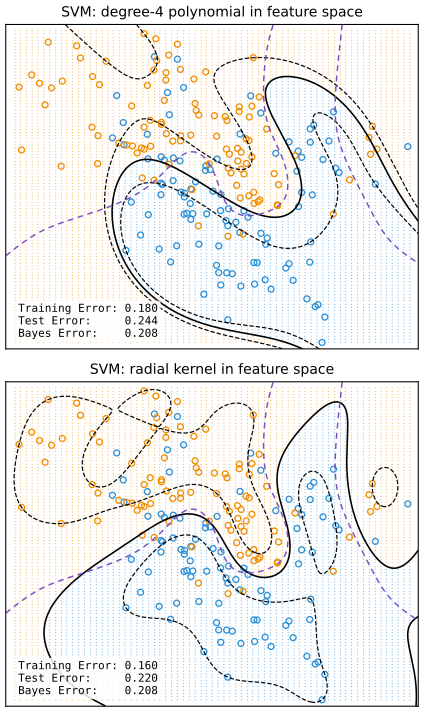
fig_12_3. Reproduces Hastie, Tibshirani and Friedman (2009), Figure 12.3. Download: PDF · SVGEarly claims that the kernel property is unique to SVMs, and that it beats the curse of dimensionality, are both false; Sections 12.3.3–12.3.4 explain why.
12.3.2 The SVM as a Penalization Method
pp. 426–428 With \(f(x)=h(x)^\T\beta+\beta_0\), consider
\[ \min_{\beta_0,\,\beta}\ \sum_{i=1}^N\big[1-y_if(x_i)\big]_++\frac\lambda2\|\beta\|^2, \tag{12.25} \]a loss plus a penalty, the form of every regularised fit in this course.
See also (companion course): Result 7.8, the SVM as hinge-loss regularisation.
Result 12.5 ((12.25) and (12.8) have the same solutions when \(\lambda=1/C\); Exercise 12.1) p. 426
For \(\lambda=1/C\), \((\hat\beta,\hat\beta_0)\) solves (12.25) if and only if it solves (12.8) (with \(\hat\xi_i=[1-y_i\hat f(x_i)]_+\)), and the optimal values satisfy \(\min(12.8)=C\cdot\min(12.25)\).
Proof
For fixed \((\beta,\beta_0)\), the constraints of (12.8) say \(\xi_i\ge0\) and \(\xi_i\ge1-y_if(x_i)\), i.e. \(\xi_i\ge[1-y_if(x_i)]_+\), and the objective increases in each \(\xi_i\). So minimising over \(\xi\) first leaves
\[ \tfrac12\|\beta\|^2+C\sum_i[1-y_if(x_i)]_+=C\{\sum_i[1-y_if(x_i)]_++\tfrac1{2C}\|\beta\|^2\} \], which is \(C\) times (12.25) with \(\lambda=1/C\). Multiplying an objective by a positive constant does not change its minimisers. ∎
The hinge loss \(L(y,f)=[1-yf]_+\) is a sensible loss for two classes. Figure 12.4 compares it, as a function of the margin \(yf\), with the binomial deviance of logistic regression, squared error, and the "Huberised" squared hinge of Rosset and Zhu (2007). The deviance has the same tails as the hinge: no loss far inside the margin, linear loss far on the wrong side. Squared error penalises both sides quadratically, so points well inside their class still pull on the fit. The squared hinge \([1-yf]_+^2\) is zero inside the margin but quadratic in the left tail, hence less robust to misclassified points; its Huberised version becomes linear at \(yf=-1\).
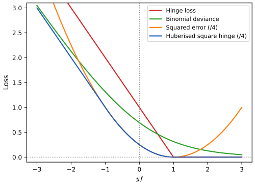
fig_12_4. Reproduces Hastie, Tibshirani and Friedman (2009), Figure 12.4. Download: PDF · SVGResult 12.6 (the population minimisers of Table 12.1) p. 427, Table 12.1
Let \(p(x)=\Pr(Y=+1\given x)\). The minimiser over \(f(x)\) of \(\E\,L[Y,f(x)]\) is, at each \(x\):
| loss | \(L[y,f(x)]\) | minimising function |
|---|---|---|
| binomial deviance | \(\log[1+e^{-yf(x)}]\) | \(\log\dfrac{p(x)}{1-p(x)}\) |
| SVM hinge loss | \([1-yf(x)]_+\) | \(\sgn[p(x)-\tfrac12]\) |
| squared error | \([y-f(x)]^2=[1-yf(x)]^2\) | \(2p(x)-1\) |
| Huberised square hinge | \(-4yf(x)\) if \(yf(x)\lt -1\); \([1-yf(x)]_+^2\) otherwise | \(2p(x)-1\) |
The hinge loss estimates the Bayes classifier itself (the mode of the posterior); the other three estimate monotone transformations of \(p(x)\), from which \(p\) can be recovered.
Proof
Conditioning on \(x\), write \(\ell(m)\) for the loss as a function of the margin \(m=yf\); then \(g(f)=\E[L\given x]=p\,\ell(f)+(1-p)\,\ell(-f)\), and all four \(\ell\) are convex, so it suffices to find a stationary point (or check the subgradient).
Deviance. \(g'(f)=-p\,\sigma(-f)+(1-p)\,\sigma(f)\) with \(\sigma(u)=1/(1+e^{-u})\); since \(\sigma(-f)=1-\sigma(f)\), \(g'(f)=\sigma(f)-p\), zero at \(\sigma(f)=p\), i.e. \(f=\log\{p/(1-p)\}\).
Hinge. \(g\) is piecewise linear with slopes \(-p\) on \((-\infty,-1)\), \(1-2p\) on \((-1,1)\) and \(1-p\) on \((1,\infty)\). If \(p>\tfrac12\) the slope changes sign at \(f=1\), the minimiser; if \(p\lt \tfrac12\) at \(f=-1\); if \(p=\tfrac12\) every \(f\in[-1,1]\) is a minimiser. So \(f^*=\sgn(p-\tfrac12)\), and \(f^*\) carries no information about \(p\) beyond which side of \(\tfrac12\) it is on.
Squared error. \(g(f)=p(1-f)^2+(1-p)(1+f)^2\),
\[ g'(f)=-2p(1-f)+2(1-p)(1+f)=2(f-2p+1) \], zero at \(f=2p-1\).
Huberised square hinge. On \(f\in[-1,1]\) both margins \(f\) and \(-f\) lie in \([-1,1]\), where \(\ell(m)=(1-m)^2\), so \(g\) equals the squared-error \(g\) there, with stationary point \(2p-1\in[-1,1]\). \(\ell\) is convex (its derivative \(-4\) for \(m\lt -1\), \(-2(1-m)\) on \([-1,1]\) and \(0\) for \(m>1\) is nondecreasing and continuous: \(-2(1-(-1))=-4\)), so this stationary point is the global minimiser. ∎
The four minimisers were confirmed numerically by a fine grid search at several values of \(p\).
The Huberised square hinge shares attractive features of both: like logistic regression it is smooth and estimates probabilities; like the SVM it has support points (zero loss beyond the margin). Formulation (12.25) shrinks all coefficients of \(h(x)^\T\beta\) uniformly toward zero (not the constant); if \(h\) is a hierarchical basis ordered by roughness, uniform shrinkage makes most sense when the rougher elements have smaller norm.
Filling the gap 12.3: margin-maximising losses, and why the limit is exact for the hinge p. 428
All the losses of Table 12.1 except squared error are "margin maximising" (Rosset, Zhu and Hastie, 2004): for separable data, as \(\lambda\to0\) the solution of (12.25) with that loss defines the optimal separating hyperplane. For the hinge loss the statement is exact for all small \(\lambda\), not just in the limit.
Derivation
Let the data be separable, let \((\beta^*,\beta_0^*)\) solve the hard-margin problem (12.4) and let \(\alpha^*\) be its multipliers (Result 4.16): \(\beta^*=\sum\alpha^*_iy_ix_i\), \(\sum\alpha_i^*y_i=0\), \(\alpha^*_i\ge0\), \(\alpha^*_i[y_if^*(x_i)-1]=0\). Take any \(C\ge\max_i\alpha^*_i\). Then \((\beta^*,\beta^*_0,\xi=0)\) with \(\alpha=\alpha^*\) and \(\mu_i=C-\alpha^*_i\ge0\) satisfies every KKT condition (12.10)–(12.16) of the soft-margin problem (12.8), which is convex, so it is the solution. By Result 12.5 it solves (12.25) for every \(\lambda\le1/\max_i\alpha^*_i\).
For the deviance the minimiser of (12.25) does not converge, \(\|\hat\beta_\lambda\|\to\infty\), but its direction \(\hat\beta_\lambda/\|\hat\beta_\lambda\|\) converges to that of the optimal separating hyperplane (the book's footnote; Rosset, Zhu and Hastie, 2004). Chapter 4 discusses what "the logistic regression solution" means for separable data (Filling the gap 4.11). Squared error is not margin maximising: its solution converges to the least-squares fit, whose boundary is usually not the maximal-margin one. ∎
12.3.3 Function Estimation and Reproducing Kernels
pp. 428–430 Suppose the basis comes from the eigen-expansion of a positive definite kernel,
\[ K(x,x')=\sum_{m=1}^\infty\phi_m(x)\phi_m(x')\delta_m, \tag{12.26} \]with \(h_m(x)=\sqrt{\delta_m}\phi_m(x)\). Writing \(\theta_m=\sqrt{\delta_m}\beta_m\), so that \(f=\beta_0+\sum\theta_m\phi_m\) and \(\|\beta\|^2=\sum\theta_m^2/\delta_m\), (12.25) becomes
\[ \min_{\beta_0,\,\theta}\ \sum_{i=1}^N\Big[1-y_i\Big(\beta_0+\sum_{m=1}^\infty\theta_m\phi_m(x_i)\Big)\Big]_++\frac\lambda2\sum_{m=1}^\infty\frac{\theta_m^2}{\delta_m}. \tag{12.27} \]See also: Section 5.8.1, spaces of functions generated by kernels, with Definition 5.4 and Result 5.13.
Result 12.7 (finite representation; Exercise 12.2) pp. 428–429, (12.28)–(12.30)
The solution of (12.27) has the form
\[ f(x)=\beta_0+\sum_{i=1}^N\alpha_iK(x,x_i), \tag{12.28} \]and \(\beta_0\), \(\alpha\) solve the finite problem
\[ \min_{\beta_0,\,\alpha}\ \sum_{i=1}^N\big(1-y_if(x_i)\big)_++\frac\lambda2\alpha^\T\bK\alpha, \tag{12.29} \]with \(\bK\) the \(N\times N\) kernel matrix. The same holds for any loss and any space \(\Hc\) of functions with a penalty \(J(f)\) that is a squared RKHS norm,
\[ \min_{f\in\Hc}\ \sum_{i=1}^N\big[1-y_if(x_i)\big]_++\lambda J(f). \tag{12.30} \]The multipliers of the dual are related by \(\alpha_i=\hat\alpha_i^{(12.24)}y_i\).
Proof
(12.27) is (5.49) of Section 5.8 with the hinge loss; the penalty \(\sum\theta_m^2/\delta_m\) is the squared norm \(\|g\|^2_{\Hc_K}\) of \(g=f-\beta_0\) in the RKHS of \(K\). The representer theorem (Result 5.13) gives \(g=\sum_i\alpha_iK(\cdot,x_i)\). For such \(g\), the reproducing property gives \(g(x_{i'})=(\bK\alpha)_{i'}\) and \(\|g\|^2=\alpha^\T\bK\alpha\), which turns (12.27) into (12.29).
A direct finite-dimensional proof (Exercise 12.2): let \(\bH\) be the \(N\times M\) matrix with rows \(h(x_i)^\T\), so \(\bK=\bH\bH^\T\). Split \(\beta=\bH^\T\alpha+\beta_\perp\) with \(\bH\beta_\perp=0\). The loss in (12.25) depends on \(\beta\) only through \(\bH\beta=\bK\alpha\), and \(\|\beta\|^2=\alpha^\T\bK\alpha+\|\beta_\perp\|^2\), so the optimum has \(\beta_\perp=0\); substituting gives (12.29), and
\[ f(x)=h(x)^\T\bH^\T\alpha+\beta_0=\sum_i\alpha_iK(x,x_i)+\beta_0 \]. Comparing with (12.17), \(\hat\beta=\sum_i\hat\alpha_iy_ih(x_i)\), shows \(\alpha_i=\hat\alpha_iy_i\) (up to the null space of \(\bK\)). Numerically, the SVM with the degree-2 kernel and the SVM on the six explicit features of (12.23) give the same \(f(x_i)\) to \(10^{-12}\). ∎
These models include smoothing splines, additive splines and interaction splines (Chapters 5 and 9; Wahba, 1990). For example, if \(\Hc\) is the space of additive functions \(f(x)=\sum_jf_j(x_j)\) with \(J(f)=\sum_j\int f_j''(x_j)^2\d x_j\), the solution of (12.30) is an additive cubic spline with kernel \(K(x,x')=\sum_jK_j(x_j,x_j')\). Conversely any kernel of (12.22) can be used with any convex loss. Figure 12.5 uses the binomial deviance with the kernels of Figure 12.3. The fitted function then estimates the log-odds,
\[ \hat f(x)=\log\frac{\hat\Pr(Y=+1\given x)}{\hat\Pr(Y=-1\given x)}=\hat\beta_0+\sum_{i=1}^N\hat\alpha_iK(x,x_i), \tag{12.31} \] \[ \hat\Pr(Y=+1\given x)=\frac1{1+e^{-\hat\beta_0-\sum_{i=1}^N\hat\alpha_iK(x,x_i)}}. \tag{12.32} \]Filling the gap 12.4: fitting kernel logistic regression p. 429
Derivation
Minimise \(Q(\beta_0,\alpha)=\sum_i\log(1+e^{-y_if_i})+\tfrac\lambda2\alpha^\T\bK\alpha\) with \(f=\beta_0\bone+\bK\alpha\). With \(t_i=(1+y_i)/2\in\{0,1\}\) and \(p_i=\sigma(f_i)\), \(\partial\log(1+e^{-y_if_i})/\partial f_i=p_i-t_i\), so
\[ \nabla_\alpha Q=\bK(\mathbf p-\mathbf t+\lambda\alpha),\qquad\partial Q/\partial\beta_0=\bone^\T(\mathbf p-\mathbf t). \]Both vanish if \(\mathbf p-\mathbf t+\lambda\alpha=0\) and \(\bone^\T(\mathbf p-\mathbf t)=0\); every solution of these \(N+1\) equations minimises \(Q\) (which is convex), and every minimiser has the same \(f\) (the null space of \(\bK\) does not change \(f\)). In particular \(\sum_i\alpha_i=0\) and \(\alpha_i=(t_i-p_i)/\lambda\): unlike the SVM, every point gets a nonzero coefficient. Newton's method on these equations, with Jacobian
\[ \begin{pmatrix}\mathbf W\bK+\lambda\bI&\mathbf W\bone\\ \bone^\T\mathbf W\bK&\bone^\T\mathbf W\bone\end{pmatrix},\qquad\mathbf W=\diag\{p_i(1-p_i)\}, \]and step halving on \(Q\), converges in a handful of iterations (kernel_logistic). It is the kernel version of the IRLS algorithm of Section 4.4. ∎
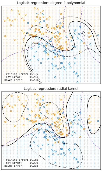
fig_12_5. Reproduces Hastie, Tibshirani and Friedman (2009), Figure 12.5. Download: PDF · SVGFor the SVM a sizeable fraction of the \(\alpha_i\) are zero: 44% and 42% for the two fits of Figure 12.3 (book: 42% and 45%). This sparsity comes from the flat part of the hinge in (12.25). The less the classes overlap on the training data, the larger the fraction; decreasing \(\lambda\) usually reduces the overlap. Fewer support points make \(\hat f\) faster to evaluate, but reducing the overlap too much overfits.
12.3.4 SVMs and the Curse of Dimensionality
pp. 431–432 A polynomial kernel is not a fully general inner product on the space of monomials: in (12.23) every term \(2X_jX_j'\) gets the same weight, and the kernel cannot learn to concentrate on a subspace. If \(p\) is large but the classes differ only in \(X_1,X_2\), the kernel spreads its effort over all the dimensions; the knowledge that only two inputs matter would have to be built into the kernel by hand. Discovering such structure is what adaptive methods try to do.
See also (companion course): Foundations of Deep Learning, Section 6.1.1, the curse of dimensionality.
The book's illustration, "the skin of the orange": class 1 has four independent standard normal features; class 2 has the same distribution conditioned on \(9\le\sum_jX_j^2\le16\), a shell around class 1. A harder version adds six standard normal noise features to both. Each training set has 100 points per class.
Filling the gap 12.5: the Bayes error 0.029 p. 431
Derivation
With equal priors, class 2 has density \(\phi(x)\bone\{9\le\|x\|^2\le16\}/q\) with \(q=\Pr(9\le\chi^2_4\le16)\), where \(\phi\) is the standard normal density of class 1. Inside the shell the class-2 density is \(\phi/q>\phi\), outside it is 0. So the Bayes rule says class 2 exactly on the shell, and its only errors are class-1 points that fall in the shell: error \(=\tfrac12q\). For \(\chi^2_4\), \(\Pr(\chi^2_4\le t)=1-e^{-t/2}(1+t/2)\), so
\[ q=e^{-4.5}(5.5)-e^{-8}(9)=0.06106-0.00302=0.05808 \]and the Bayes error is \(0.02904\). The noise features are independent of the class, so they do not change it. ∎
Table 12.2. Skin of the orange: mean test error (standard error) over 50 simulations p. 431
| method | no noise: ours | book | six noise features: ours | book |
|---|---|---|---|---|
| 1 SV classifier | 0.425 (0.002) | 0.450 (0.003) | 0.468 (0.003) | 0.472 (0.003) |
| 2 SVM/poly 2 | 0.053 (0.001) | 0.078 (0.003) | 0.098 (0.002) | 0.152 (0.004) |
| 3 SVM/poly 5 | 0.142 (0.003) | 0.180 (0.004) | 0.296 (0.003) | 0.370 (0.004) |
| 4 SVM/poly 10 | 0.159 (0.003) | 0.230 (0.003) | 0.375 (0.003) | 0.434 (0.002) |
| 5 additive splines (BRUTO in the book) | 0.064 (0.002) | 0.084 (0.003) | 0.083 (0.002) | 0.090 (0.003) |
| 6 MARS | 0.115 (0.003) | 0.156 (0.004) | 0.135 (0.003) | 0.173 (0.005) |
| Bayes | 0.029 | 0.029 | 0.029 | 0.029 |
Our settings: 100 training points per class, 500 test points per class; for the SVMs the kernel (12.22) and \(C\) chosen from 13 values in \([10^{-3},10^3]\) to minimise the test error, as in the book; line 5 is least squares on additive natural splines with 4 df per input (in place of the adaptive BRUTO); line 6 is MARS with interactions of all orders (orange_table). Our errors are a little lower throughout, but the pattern is the book's.
A hyperplane cannot separate the classes (line 1). The polynomial SVMs do much better, but the six noise features hurt them badly, and they are very sensitive to the degree: degree 2 is best because the true boundary \(\|x\|^2=\) constant is a quadratic, and higher degrees are worse. The additive model fits well because the boundary is additive in the \(X_j^2\), and both it and MARS can ignore the redundant inputs, so they barely suffer from the noise features. The kernel has to treat all ten inputs alike.
12.3.5 A Path Algorithm for the SVM Classifier
pp. 432–434 The cost \(C\) (or \(\lambda=1/C\)) matters, and its best value depends strongly on the kernel. Figure 12.6 shows the test error of the radial SVM on the mixture data as a function of \(C\) for four kernel widths: with narrow kernels (\(\gamma=5\)) heavy regularisation is needed; with \(\gamma=1\) an intermediate \(C\).
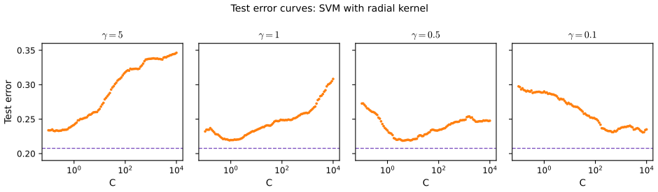
fig_12_6, test_error_curves. Reproduces Hastie, Tibshirani and Friedman (2009), Figure 12.6. Download: PDF · SVGRather than refit at a grid of values, one can follow the solution as \(\lambda\) changes (in the spirit of LARS, Section 3.8). In the loss + penalty form (12.25) the solution at \(\lambda\) is
\[ \beta_\lambda=\frac1\lambda\sum_{i=1}^N\alpha_iy_ix_i, \tag{12.33} \]where the \(\alpha_i\) are again Lagrange multipliers, now in \([0,1]\); with a kernel,
\[ f_\lambda(x)=\frac1\lambda\sum_{i=1}^N\alpha_iy_iK(x,x_i)\ \ (+\beta_0). \tag{12.34} \]Result 12.8 (the SVM path is piecewise linear) pp. 433–434
Write \(\alpha_0=\lambda\beta_0\), so \(\lambda f_\lambda(x)=\sum_j\alpha_jy_jK(x,x_j)+\alpha_0\). The KKT conditions of (12.25) split the points into three sets:
- \(\mathcal R\): \(y_if(x_i)>1\) (correct side, outside the margin), \(\alpha_i=0\);
- \(\mathcal E\) (the elbow): \(y_if(x_i)=1\), \(\alpha_i\in[0,1]\);
- \(\mathcal L\): \(y_if(x_i)\lt 1\) (inside the margin or misclassified), \(\alpha_i=1\).
Between events at which a point changes set, \(\alpha_{\mathcal E}(\lambda)\) and \(\alpha_0(\lambda)\) are linear in \(\lambda\) and the other \(\alpha_i\) are constant, so every \(\alpha_i(\lambda)\) is piecewise linear. The direction of change solves the \((|\mathcal E|+1)\)-dimensional system
\[ \sum_{j\in\mathcal E}y_jK(x_i,x_j)\,b_j+b_0=y_i\ \ (i\in\mathcal E),\qquad\sum_{j\in\mathcal E}y_jb_j=0,\qquad b_j=\frac{\d\alpha_j}{\d\lambda},\ b_0=\frac{\d\alpha_0}{\d\lambda}. \]With equal class sizes, for all large \(\lambda\) every \(\alpha_i=1\); the path starts at \(\lambda_0=\tfrac12(g_{i_+}-g_{i_-})\), where \(g_i=\sum_jy_jK(x_i,x_j)\), \(i_+\) maximises \(g_i\) over the class \(+1\) and \(i_-\) minimises it over the class \(-1\); there \(\alpha_0=-\tfrac12(g_{i_+}+g_{i_-})\) and \(\mathcal E=\{i_+,i_-\}\).
Proof and the algorithm
KKT conditions. Write (12.25) as \(\min\sum_i\xi_i+\tfrac\lambda2\|\beta\|^2\) subject to \(\xi_i\ge1-y_if(x_i)\), \(\xi_i\ge0\). With multipliers \(\alpha_i\) and \(\gamma_i\), stationarity gives \(\lambda\beta=\sum_i\alpha_iy_ih(x_i)\) (which is (12.33)), \(\sum_i\alpha_iy_i=0\) and \(1-\alpha_i-\gamma_i=0\), so \(\alpha_i\in[0,1]\). The case analysis of Result 12.2 with \(C\) replaced by 1 gives the three sets. Multiplying \(f\) by \(\lambda\), \(h_i(\lambda):=\lambda f_\lambda(x_i)=\sum_j\alpha_jy_jK_{ij}+\alpha_0\).
Linearity. Fix the three sets. The unknowns \(\alpha_{\mathcal E},\alpha_0\) must satisfy \(y_ih_i=\lambda\) for \(i\in\mathcal E\) (i.e. \(h_i=\lambda y_i\)) and \(\sum\alpha_jy_j=0\):
\[ \sum_{j\in\mathcal E}y_jK_{ij}\alpha_j+\alpha_0=\lambda y_i-\sum_{j\in\mathcal L}y_jK_{ij}\ \ (i\in\mathcal E),\qquad\sum_{j\in\mathcal E}y_j\alpha_j=-\sum_{j\in\mathcal L}y_j. \]The right-hand side is affine in \(\lambda\), so if the \((|\mathcal E|+1)\times(|\mathcal E|+1)\) matrix is nonsingular the solution is affine in \(\lambda\), with derivative given by the system in the statement (differentiate both sides). Then every \(h_i(\lambda)\) is affine in \(\lambda\) too. The solution in \(f\) of the strictly convex problem (12.25) is continuous in \(\lambda\), so the pieces join continuously: the path is piecewise linear, with breakpoints where the sets change.
Events. Decreasing \(\lambda\) by \(\delta\) moves \(\alpha_j\to\alpha_j-\delta b_j\) (\(j\in\mathcal E\)) and \(h_i\to h_i-\delta\,\dot h_i\) with \(\dot h_i=\sum_{j\in\mathcal E}y_jK_{ij}b_j+b_0\). The next breakpoint is the smallest \(\delta>0\) at which (a) some \(\alpha_j\), \(j\in\mathcal E\), reaches 0 (the point leaves to \(\mathcal R\)) or 1 (to \(\mathcal L\)): \(\delta=\alpha_j/b_j\) or \((\alpha_j-1)/b_j\); or (b) a point of \(\mathcal L\) or \(\mathcal R\) reaches its margin, \(y_i(h_i-\delta\dot h_i)=\lambda-\delta\), i.e. \(\delta=(\lambda-y_ih_i)/(1-y_i\dot h_i)\). Update the sets and repeat until \(\lambda\) reaches the smallest value wanted (or \(\mathcal L\) is empty: the data are separated). By continuity a point moving between \(\mathcal L\) and \(\mathcal R\) always passes through \(\mathcal E\), lingering on the margin while its \(\alpha\) runs from 1 to 0.
Start. If all \(\alpha_i=1\), \(\sum\alpha_iy_i=0\) needs equal class sizes, and \(h_i=g_i+\alpha_0\). Feasibility is \(y_ih_i\le\lambda\) for all \(i\): \(g_i+\alpha_0\le\lambda\) on the class \(+1\) and \(-g_i-\alpha_0\le\lambda\) on the class \(-1\), i.e. \(-\lambda-\min_{-}g\le\alpha_0\le\lambda-\max_{+}g\). This interval is nonempty for \(\lambda\ge\lambda_0=\tfrac12(\max_+g-\min_-g)\) and collapses to the single \(\alpha_0\) of the statement at \(\lambda_0\), where both extreme points reach their margins. (Unequal class sizes need a different start; Hastie, Rosset, Tibshirani and Zhu, 2004.)
Size of the elbow. The first block of the system maps into the span of the columns of \([\bH_{\mathcal E},\bone]\), so the matrix is singular once \(|\mathcal E|\) exceeds \(D=\dim\span\{h_1,\dots,h_M,1\}\): for a linear kernel in \(\R^p\) at most \(p+1\) points are on the margin at once (3 in Figure 12.2), 15 for the degree-4 kernel in \(\R^2\) (the 15 monomials of degree at most 4), and up to \(N\) for the radial kernel. Each step costs one solve of size \(|\mathcal E|+1\) and \(O(N|\mathcal E|)\) updates. ∎
The course code (svm_path) implements exactly this. On the mixture data it takes 171 breakpoints for the linear kernel, 417 for the degree-4 kernel and 625 for the radial kernel with \(\gamma=1\) to go from \(\lambda_0\) down to \(\lambda=10^{-4}\), in well under a second, and its solutions agree with an independent SMO solver and with LIBSVM; the KKT conditions hold to \(10^{-10}\) along the whole path.
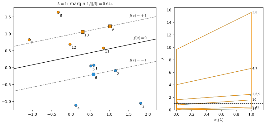
fig_12_7. Reproduces Hastie, Tibshirani and Friedman (2009), Figure 12.7. Download: PDF · SVGNote on the book: two inconsistencies around Figure 12.7
The caption first says the left panel shows the model "at \(\lambda=0.05\)" and then "\(\lambda=1/2\)"; the right panel marks \(\lambda=1/2\), which is the value meant. In the text, the points on their margins are listed as "the orange 7 and the blue 2 and 8", but 8 is orange and is listed two lines earlier among the points outside their margins; the caption's square points \(\{2,6,7\}\) show that "blue 2 and 6" is meant.
12.3.6 Support Vector Machines for Regression
pp. 434–436 For a quantitative response, take the linear model
\[ f(x)=x^\T\beta+\beta_0 \tag{12.35} \]and minimise
\[ H(\beta,\beta_0)=\sum_{i=1}^NV(y_i-f(x_i))+\frac\lambda2\|\beta\|^2, \tag{12.36} \]with the \(\epsilon\)-insensitive loss
\[ V_\epsilon(r)=\begin{cases}0&\text{if }|r|\lt \epsilon,\\ |r|-\epsilon&\text{otherwise,}\end{cases} \tag{12.37} \]which ignores errors smaller than \(\epsilon\), as the SVM classifier ignores points well inside their margin. Compare Huber's (1964) robust loss
\[ V_H(r)=\begin{cases}r^2/2&\text{if }|r|\le c,\\ c|r|-c^2/2,&|r|>c,\end{cases} \tag{12.38} \]quadratic for small residuals and linear beyond \(c\), which limits the influence of outliers. \(V_\epsilon\) also has linear tails but in addition flattens the small residuals.
See also (companion course): Section 7.1.4, SVMs for regression, and Result 7.9.
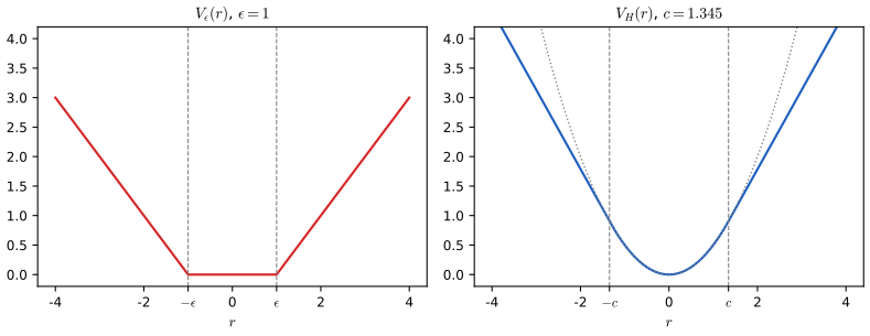
fig_12_8. Reproduces Hastie, Tibshirani and Friedman (2009), Figure 12.8. Download: PDF · SVGResult 12.9 (the dual of support vector regression) pp. 435–436, (12.39)–(12.41)
The minimisers of (12.36) with \(V=V_\epsilon\) are
\[ \hat\beta=\sum_{i=1}^N(\hat\alpha^*_i-\hat\alpha_i)x_i, \tag{12.39} \] \[ \hat f(x)=\sum_{i=1}^N(\hat\alpha^*_i-\hat\alpha_i)\langle x,x_i\rangle+\beta_0, \tag{12.40} \]where \(\hat\alpha_i,\hat\alpha^*_i\ge0\) solve
\[ \min_{\alpha_i,\alpha_i^*}\ \epsilon\sum_{i=1}^N(\alpha^*_i+\alpha_i)-\sum_{i=1}^Ny_i(\alpha^*_i-\alpha_i)+\frac12\sum_{i,i'=1}^N(\alpha^*_i-\alpha_i)(\alpha^*_{i'}-\alpha_{i'})\langle x_i,x_{i'}\rangle \] \[ \text{subject to}\quad0\le\alpha_i,\alpha^*_i\le1/\lambda,\quad\sum_{i=1}^N(\alpha^*_i-\alpha_i)=0,\quad\alpha_i\alpha^*_i=0. \tag{12.41} \]Points with \(|y_i-\hat f(x_i)|\lt \epsilon\) have \(\hat\alpha_i=\hat\alpha^*_i=0\); points outside the tube have \(|\hat\alpha^*_i-\hat\alpha_i|=1/\lambda\). The last constraint holds automatically at the optimum and can be dropped.
Proof
Multiply (12.36) by \(C=1/\lambda\) and introduce slacks: minimise \(\tfrac12\|\beta\|^2+C\sum_i(\xi_i+\xi^*_i)\) subject to \(y_i-f(x_i)\le\epsilon+\xi^*_i\), \(f(x_i)-y_i\le\epsilon+\xi_i\), \(\xi_i,\xi^*_i\ge0\) (at the optimum \(\xi^*_i=[y_i-f_i-\epsilon]_+\), \(\xi_i=[f_i-y_i-\epsilon]_+\), and their sum is \(V_\epsilon(y_i-f_i)\)). With multipliers \(\alpha^*_i,\alpha_i,\eta^*_i,\eta_i\ge0\) the Lagrangian is
\[ \tfrac12\|\beta\|^2+C\sum(\xi_i+\xi_i^*)-\sum\alpha^*_i(\epsilon+\xi^*_i-y_i+f_i)-\sum\alpha_i(\epsilon+\xi_i+y_i-f_i)-\sum(\eta_i\xi_i+\eta^*_i\xi^*_i). \]Stationarity: \(\beta=\sum(\alpha^*_i-\alpha_i)x_i\) (12.39), \(\sum(\alpha_i^*-\alpha_i)=0\), \(C-\alpha^*_i-\eta^*_i=0\) and \(C-\alpha_i-\eta_i=0\), so \(0\le\alpha_i,\alpha^*_i\le C=1/\lambda\). Substituting, the terms in \(\beta_0\), \(\xi\) and \(\xi^*\) vanish and the dual function is
\[ -\tfrac12\|\sum(\alpha^*_i-\alpha_i)x_i\|^2-\epsilon\sum(\alpha^*_i+\alpha_i)+\sum y_i(\alpha^*_i-\alpha_i) \]; maximising it is minimising its negative, which is the objective of (12.41). (12.40) is \(x^\T\hat\beta+\beta_0\).
Complementary slackness. \(\alpha^*_i>0\) requires \(y_i-f_i=\epsilon+\xi^*_i\ge\epsilon\) and \(\alpha_i>0\) requires \(f_i-y_i=\epsilon+\xi_i\ge\epsilon\); for \(\epsilon>0\) both cannot happen (adding them would give \(0\ge2\epsilon\)), so \(\alpha_i\alpha^*_i=0\) at every optimum. Inside the tube neither constraint is active, so both multipliers vanish: these points are not support vectors. Outside it the slack is positive, so \(\eta=0\) and the multiplier equals \(C\). These relations, and the equality of the primal and dual optimal values, were confirmed numerically on simulated data. ∎
As in classification the solution depends on the inputs only through inner products, so any kernel of (12.22) can be used. The two parameters play different roles: \(\epsilon\) belongs to the loss, like \(c\) to Huber's; \(\lambda\) is an ordinary regularisation parameter, to be chosen for example by cross-validation. Both \(V_\epsilon\) and \(V_H\) depend on the scale of \(y\); after scaling the residuals by an estimate \(\hat\sigma\), preset values can be used, and \(c=1.345\) gives 95% efficiency at the Gaussian.
Filling the gap 12.6: why \(c=1.345\) gives 95% efficiency p. 436
Derivation
For a location model with standard Gaussian errors, an M-estimator with score \(\psi=V'\) has asymptotic variance \(\E\psi(Z)^2/\{\E\psi'(Z)\}^2\) (Huber, 1964), against 1 for the mean. For Huber's loss \(\psi(z)=\max(-c,\min(c,z))\), \(\psi'(z)=\bone\{|z|\lt c\}\). With \(\Phi,\phi\) the standard normal distribution and density:
\[ \E\psi'(Z)=2\Phi(c)-1,\qquad\E\psi(Z)^2=\int_{-c}^cz^2\phi\,\d z+2c^2\{1-\Phi(c)\}=\{2\Phi(c)-1\}-2c\phi(c)+2c^2\{1-\Phi(c)\}, \]using \(\int_{-c}^cz^2\phi=\{2\Phi(c)-1\}-2c\phi(c)\) (integrate by parts with \(z\phi=-\phi'\)). The efficiency is \(\{2\Phi(c)-1\}^2/\E\psi^2\); at \(c=1.345\) it is \(0.9500\). ∎
12.3.7 Regression and Kernels
pp. 436–437 The kernel property is not special to SVMs. Approximate the regression function with basis functions \(h_m\), \(m=1,\dots,M\),
\[ f(x)=\sum_{m=1}^M\beta_mh_m(x)+\beta_0, \tag{12.42} \]and minimise, for a general error measure \(V\),
\[ H(\beta,\beta_0)=\sum_{i=1}^NV(y_i-f(x_i))+\frac\lambda2\sum\beta_m^2. \tag{12.43} \]For any \(V\) the solution has the form
\[ \hat f(x)=\sum_{i=1}^N\hat a_iK(x,x_i) \tag{12.44} \](plus the constant) with \(K(x,y)=\sum_{m=1}^Mh_m(x)h_m(y)\), by the argument of Result 12.7. For squared error, with \(\bH\) the \(N\times M\) basis matrix, \(M>N\) and the constant absorbed into \(h\) (see Exercise 12.3 for an unpenalised constant), minimise
\[ H(\beta)=(\by-\bH\beta)^\T(\by-\bH\beta)+\lambda\|\beta\|^2. \tag{12.45} \]Result 12.10 (kernel ridge regression) p. 437, (12.46)–(12.49)
The solution \(\hat\by=\bH\hat\beta\) (12.46), with \(\hat\beta\) determined by
\[ -\bH^\T(\by-\bH\hat\beta)+\lambda\hat\beta=0, \tag{12.47} \]can be computed from the \(N\times N\) matrix \(\bH\bH^\T\) alone:
\[ \bH\hat\beta=(\bH\bH^\T+\lambda\bI)^{-1}\bH\bH^\T\by, \tag{12.48} \]\(\{\bH\bH^\T\}_{ii'}=K(x_i,x_{i'})\), and at any \(x\)
\[ \hat f(x)=h(x)^\T\hat\beta=\sum_{i=1}^N\hat\alpha_iK(x,x_i),\qquad\hat\alpha=(\bH\bH^\T+\lambda\bI)^{-1}\by. \tag{12.49} \]Proof
(12.47) is the gradient of (12.45) set to zero (divided by 2). It says \(\hat\beta=\bH^\T\hat\alpha\) with \(\hat\alpha=(\by-\bH\hat\beta)/\lambda\): the solution lies in the row space of \(\bH\). Then \(\lambda\hat\alpha=\by-\bH\bH^\T\hat\alpha\), so \((\bH\bH^\T+\lambda\bI)\hat\alpha=\by\), which is (12.49), and \(\bH\hat\beta=\bH\bH^\T\hat\alpha\) is (12.48) (the two matrices commute). Equivalently, the push-through identity \((\bH^\T\bH+\lambda\bI)^{-1}\bH^\T=\bH^\T(\bH\bH^\T+\lambda\bI)^{-1}\), obtained by multiplying \(\bH^\T(\bH\bH^\T+\lambda\bI)=(\bH^\T\bH+\lambda\bI)\bH^\T\) by the two inverses, turns the \(M\times M\) solve into an \(N\times N\) one. ∎
So, as for the SVM, the large set of functions \(h_1,\dots,h_M\) never has to be evaluated, only the kernel at the \(N^2\) pairs of training points (\(N^2/2\) evaluations by symmetry, instead of \(N^2M\) operations) and at new points. This depends on the squared norm in the penalty: with an \(L_1\) penalty \(\sum|\beta_m|\), which may give a better model, the solution is no longer in the row space of \(\bH\).
See also (companion course): Section 6.1, dual representations, the same computation from the Bayesian side.
12.3.8 Discussion
p. 438 For \(K>2\) classes the SVM is usually applied to pairs of classes, with the final rule the class that wins most pairwise contests (Kressel, 1999; Friedman, 1996; Hastie and Tibshirani, 1998); alternatively the multinomial deviance with a kernel can be used as in Section 12.3.3 (companion course, Section 7.1.3).
The SVM also connects with structural risk minimisation (7.9). Suppose the training points (or their features) lie in a ball of radius \(R\), and \(G(x)=\sgn[f(x)]=\sgn[\beta^\T x+\beta_0]\). Then the class \(\{G(x),\ \|\beta\|\le A\}\) has VC dimension \(h\) satisfying
\[ h\le R^2A^2. \tag{12.50} \]If \(f\) separates the training data, optimally for \(\|\beta\|\le A\), then with probability at least \(1-\eta\) over training sets (Vapnik, 1996, p. 139),
\[ \text{Error}_{\text{Test}}\le4\,\frac{h[\log(2N/h)+1]-\log(\eta/4)}{N}. \tag{12.51} \]Result 12.11 (the margin bound on the VC dimension) p. 438, (12.50)
Let \(x_1,\dots,x_h\) lie in the ball \(\|x\|\le R\). If for every labelling \(y\in\{-1,1\}^h\) there is a \(\beta\) with \(\|\beta\|\le A\) and \(y_i\beta^\T x_i\ge1\) for all \(i\) (the points are shattered with margin \(1/A\)), then \(h\le R^2A^2\).
Proof
For a labelling \(y\) and its \(\beta\), summing \(y_i\beta^\T x_i\ge1\) gives \(\beta^\T\sum_iy_ix_i\ge h\), so by Cauchy–Schwarz \(\|\sum_iy_ix_i\|\ge h/\|\beta\|\ge h/A\). Now average \(\|\sum_iy_ix_i\|^2\) over the \(2^h\) labellings: the cross terms \(y_iy_jx_i^\T x_j\) (\(i\ne j\)) average to zero, so the average is \(\sum_i\|x_i\|^2\le hR^2\). Some labelling is at most the average, hence \(h^2/A^2\le hR^2\), i.e. \(h\le R^2A^2\). ∎
This is the version for hyperplanes through the origin with margin defined by \(\|\beta\|\); Vapnik's statement for affine hyperplanes is \(h\le\min(R^2A^2,p)+1\). The bound (12.51) is the VC generalisation bound of Chapter 7 with this \(h\) inserted; its proof is in Vapnik (1996).
The support vector classifier was one of the first practical procedures with a useful bound on its VC dimension, so that structural risk minimisation could be carried out: \(C\) controls an upper bound on the VC dimension, and one could choose \(C\) by minimising (12.51). Two caveats: the ball is drawn around the observed features, so in a strict sense the VC dimension is not fixed before seeing the data; and it is not clear that this beats cross-validation for choosing \(C\). See the companion course, Section 7.1.5, for PAC bounds.
12.4 Generalizing Linear Discriminant Analysis
pp. 438–440 LDA (Section 4.3) has real virtues. It is a simple prototype classifier: classify to the nearest class centroid in the Mahalanobis metric of the pooled covariance. It is the estimated Bayes rule when the classes are Gaussian with a common covariance. Its boundaries are linear and easy to describe. It gives natural low-dimensional views of the data (Figure 12.12 is a two-dimensional view of 256-dimensional digits). And its low variance often makes it the best classifier in practice: it was among the top three for 11 of the 22 data sets of the STATLOG project (Michie, Spiegelhalter and Taylor, 1994).
It fails in three typical situations: the boundaries need to be nonlinear; one prototype per class is not enough to describe the class; or there are too many correlated predictors (signals, images), so that the LDA coefficients are estimated with high variance. The rest of the chapter answers each with one idea: recast LDA as a regression and make the regression flexible (FDA); penalise the coefficients so that they are smooth (PDA); model each class by a mixture of Gaussians with a common covariance (MDA).
See also: Section 4.3 and 4.3.3 (LDA and its reduced-rank form); companion course Section 4.1.6, Fisher's discriminant for multiple classes.
12.5 Flexible Discriminant Analysis
pp. 440–444 Let \(\theta:\{1,\dots,K\}\to\R\) assign a score to each class, chosen so that the transformed labels are predicted as well as possible by linear regression on \(X\):
\[ \min_{\beta,\theta}\ \sum_{i=1}^N\big(\theta(g_i)-x_i^\T\beta\big)^2, \tag{12.52} \]with restrictions on \(\theta\) (mean zero, unit variance over the training data) to avoid the trivial solution. More generally take \(L\le K-1\) mutually orthogonal scorings \(\theta_1,\dots,\theta_L\) and maps \(\eta_\ell(X)=X^\T\beta_\ell\), chosen to minimise the average squared residual
\[ \ASR=\frac1N\sum_{\ell=1}^L\Big[\sum_{i=1}^N\big(\theta_\ell(g_i)-x_i^\T\beta_\ell\big)^2\Big]. \tag{12.53} \]The reason for this detour is the following pair of facts.
See also (companion course): Result 4.5, Fisher's discriminant is least squares with special targets (two classes).
Result 12.12 (optimal scoring is LDA; Exercise 12.8) p. 441
Let \(\ST,\SB,\SW\) be the total, between- and within-class covariance matrices (divisor \(N\)), \(\Dpi=\diag(\pi_k)\) the class proportions and \(\bM\) the \(K\times p\) matrix of centred class means. The optimal scores (normalised \(\theta^\T\Dpi\theta=1\), mean zero) are the generalised eigenvectors
\[ \Dpi\bM\ST^{-1}\bM^\T\Dpi\,\theta_\ell=\alpha_\ell^2\,\Dpi\theta_\ell,\qquad\alpha_1^2\ge\alpha_2^2\ge\cdots, \]with mean squared residual \(r^2_\ell=1-\alpha^2_\ell\), and the regression coefficients \(\beta_\ell=\ST^{-1}\bM^\T\Dpi\theta_\ell\) satisfy
\[ \SB\beta_\ell=\frac{\alpha^2_\ell}{1-\alpha^2_\ell}\,\SW\beta_\ell,\qquad\beta_\ell^\T\SW\beta_\ell=r^2_\ell(1-r^2_\ell). \]So \(\beta_\ell=\sqrt{r^2_\ell(1-r^2_\ell)}\;\nu_\ell\), where \(\nu_\ell\) is the \(\ell\)-th discriminant (canonical) direction of Section 4.3.3, normalised by \(\nu^\T\SW\nu=1\), and its eigenvalue is \(\alpha^2_\ell/(1-\alpha^2_\ell)\).
Proof
Centre the inputs (the regression has an intercept, which absorbs the means). Then \(\bX^\T\bY/N=\bM^\T\Dpi\) (column \(k\) is \(\pi_k\mu_k\)), \(\ST=\bX^\T\bX/N\), \(\SB=\bM^\T\Dpi\bM\) and \(\ST=\SW+\SB\) (the divisor-\(N\) versions of the decomposition in Filling the gap 4.6).
The scores. For a score vector \(\theta\) with \(\bone^\T\Dpi\theta=0\), the response \(\bY\theta\) has mean zero, so the intercept is 0 and the least-squares slope is \(\beta=(\bX^\T\bX)^{-1}\bX^\T\bY\theta=\ST^{-1}\bM^\T\Dpi\theta\). The mean squared residual is
\[ \tfrac1N\|\bY\theta-\bX\beta\|^2=\theta^\T\Dpi\theta-\theta^\T\Dpi\bM\ST^{-1}\bM^\T\Dpi\theta, \]using \(\bY^\T\bY/N=\Dpi\) and
\[ \|\bY\theta-\bS\bY\theta\|^2=\theta^\T\bY^\T(\bI-\bS)\bY\theta \]for the projection \(\bS\). Under \(\theta^\T\Dpi\theta=1\), minimising the residual is maximising the Rayleigh quotient of \(\Dpi\bM\ST^{-1}\bM^\T\Dpi\) relative to \(\Dpi\): the solutions are the generalised eigenvectors, the minimal residual is \(r^2=1-\alpha^2\), and successive scores are \(\Dpi\)-orthogonal. (The constant vector is also an eigenvector, with eigenvalue 0 here because \(\bM^\T\pi=0\) for centred means; with the intercept included it has eigenvalue 1 and is the trivial score.)
The coefficients. With \(\beta=\ST^{-1}\bM^\T\Dpi\theta\),
\[ \SB\beta=\bM^\T\Dpi\bM\ST^{-1}\bM^\T\Dpi\theta=\bM^\T(\alpha^2\Dpi\theta)=\alpha^2\ST\beta. \]Since \(\ST=\SW+\SB\), \(\SB\beta=\alpha^2(\SW+\SB)\beta\), i.e. \((1-\alpha^2)\SB\beta=\alpha^2\SW\beta\): \(\beta\) solves Fisher's generalised eigenproblem (Result 4.6) with eigenvalue \(\alpha^2/(1-\alpha^2)\), an increasing function of \(\alpha^2\), so the orderings agree. For the normalisation, \(\beta^\T\ST\beta=\theta^\T\Dpi\bM\ST^{-1}\bM^\T\Dpi\theta=\alpha^2\), \(\beta^\T\SB\beta=\alpha^2\beta^\T\ST\beta=\alpha^4\), so \(\beta^\T\SW\beta=\alpha^2-\alpha^4=r^2(1-r^2)\). (Distinct scores are \(\Dpi\)-orthogonal, so the \(\beta\)'s are \(\ST\)- and hence \(\SW\)-orthogonal, as discriminant directions are.) ∎
On the vowel data the ten ratios \(\beta_\ell/\nu_\ell\) are constant across coordinates and equal to \(\sqrt{r^2_\ell(1-r^2_\ell)}\) to \(10^{-12}\), and \(\alpha^2_\ell/(1-\alpha^2_\ell)\) reproduces the LDA eigenvalues (4.052, 2.538, 0.321, ...).
Result 12.13 (Mahalanobis distances from the fits) p. 441, (12.54)–(12.55)
With \(\hat\eta_\ell(x)=x^\T\beta_\ell\) and \(\bar\eta^k_\ell\) the mean of \(\hat\eta_\ell(x_i)\) over class \(k\), the Mahalanobis distance of \(x\) to the \(k\)-th class centroid in the metric \(\SW^{-1}\) is
\[ \delta_J(x,\hat\mu_k)=\sum_{\ell=1}^{K-1}w_\ell\big(\hat\eta_\ell(x)-\bar\eta^k_\ell\big)^2+D(x), \tag{12.54} \] \[ w_\ell=\frac1{r^2_\ell(1-r^2_\ell)}, \tag{12.55} \]where \(D(x)\) does not depend on \(k\). So LDA is: \(K-1\) linear regressions on optimal scores, then classification to the nearest centroid in the space of fits, with these weights; using only the first \(L\) fits gives reduced-rank LDA.
Proof
Complete the discriminant directions to a basis \(\nu_1,\dots,\nu_p\) of generalised eigenvectors of \((\SB,\SW)\) with \(\nu_\ell^\T\SW\nu_{\ell'}=\delta_{\ell\ell'}\). With \(\bm V=(\nu_1,\dots,\nu_p)\), \(\bm V^\T\SW\bm V=\bI\), so \(\SW^{-1}=\bm V\bm V^\T\) and
\[ (x-\hat\mu_k)^\T\SW^{-1}(x-\hat\mu_k)=\sum_{\ell=1}^p\big(\nu_\ell^\T(x-\hat\mu_k)\big)^2. \]For \(\ell\ge K\) the eigenvalue is 0: \(0=\nu_\ell^\T\SB\nu_\ell=\sum_k\pi_k(\nu_\ell^\T\hat\mu_k)^2\) (centred means), so \(\nu_\ell^\T\hat\mu_k=0\) for all \(k\) and these terms are \((\nu_\ell^\T x)^2\), which make up \(D(x)\). For \(\ell\le K-1\), by Result 12.12, \(\nu_\ell=\beta_\ell/\sqrt{r_\ell^2(1-r_\ell^2)}\), and \(\beta_\ell^\T\hat\mu_k=\bar\eta^k_\ell\) (the mean of a linear function), so \(\big(\nu_\ell^\T(x-\hat\mu_k)\big)^2=w_\ell(\hat\eta_\ell(x)-\bar\eta^k_\ell)^2\). ∎
Two details: the weights correspond to \(\SW\) with divisor \(N\) (with \(N-K\) every distance is multiplied by \((N-K)/N\), which matters only through the prior term \(-2\log\pi_k\)); and an intercept in \(\hat\eta_\ell\) cancels in the differences. On the vowel test data the distances from (12.54) and from LDA differ by a term that does not depend on the class, to \(4\times10^{-13}\), and the classifications coincide.
The real point is the generalisation it invites: replace the linear fits \(\eta_\ell(x)=x^\T\beta_\ell\) by nonparametric ones (additive models, splines, MARS, kernels), chosen to minimise
\[ \ASR\big(\{\theta_\ell,\eta_\ell\}_{\ell=1}^L\big)=\frac1N\sum_{\ell=1}^L\Big[\sum_{i=1}^N\big(\theta_\ell(g_i)-\eta_\ell(x_i)\big)^2+\lambda J(\eta_\ell)\Big], \tag{12.56} \]with \(J\) a regulariser (smoothing splines, additive splines, low-order ANOVA splines, or an RKHS norm as in Section 12.3.3), and classify with (12.54)–(12.55) in the space of fits. A simple case: degree-2 polynomial regression for each \(\eta_\ell\) gives quadratic decision boundaries. The same boundaries come from LDA on the inputs augmented by their squares and cross-products: linear boundaries in the enlarged space are quadratic in the original one. FDA is LDA in the enlarged space (penalised LDA when \(J\neq0\), Section 12.6), the same paradigm as the SVM.
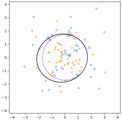
fig_12_9. Reproduces Hastie, Tibshirani and Friedman (2009), Figure 12.9. Download: PDF · SVGFilling the gap 12.7: why the boundaries are quadratic, and the Bayes sphere p. 442
Derivation
Quadratic boundaries. Each \(\hat\eta_\ell\) is a quadratic polynomial in \(x\), and \(\bar\eta^k_\ell\) a constant. In (12.54) the comparison between classes \(k\) and \(k'\) is
\[ \sum_\ell w_\ell[(\hat\eta_\ell-\bar\eta^k_\ell)^2-(\hat\eta_\ell-\bar\eta^{k'}_\ell)^2]=\sum_\ell w_\ell[2\hat\eta_\ell(\bar\eta^{k'}_\ell-\bar\eta^k_\ell)+(\bar\eta^k_\ell)^2-(\bar\eta^{k'}_\ell)^2] \]: the squares \(\hat\eta_\ell^2\) cancel and the difference is linear in the \(\hat\eta_\ell\), hence a quadratic polynomial in \(x\). By Result 12.13 applied to the basis \(h(x)=(x,x^2,\dots)\), this is LDA on \(h(x)\).
The Bayes boundary. With equal priors,
\[ \log\phi(x;0,\bI)-\log\phi(x;0,c\bI)=-\tfrac12\|x\|^2+\tfrac1{2c}\|x\|^2+\tfrac p2\log c \], which vanishes when \(\tfrac12\|x\|^2(1-\tfrac1c)=\tfrac p2\log c\), i.e.
\[ \|x\|^2=\frac{p\,c\log c}{c-1}. \]In the enlarged space this is the hyperplane \(x_1^2+\cdots+x_p^2=\) constant. ∎
Note on the book: the radius of the Bayes sphere
The text gives the Bayes boundary as \(\|x\|=\dfrac{pc\log c}{2(c-1)}\). The correct statement (Filling the gap 12.7) is \(\|x\|^2=\dfrac{pc\log c}{c-1}\). For Figure 12.9 (\(p=2\), \(c=9/4\)) the printed formula gives 1.460, while the true radius is 1.709, which is what the purple circle in the book's figure shows (it crosses the axes near \(\pm1.7\)). A numerical root of the density equation confirms 1.7086.
Many nonparametric regressions work by building a basis of derived variables and regressing on it: MARS (Chapter 9) explicitly; smoothing and additive splines with very large bases (\(N\times p\) functions for additive splines) and a penalty; kernel methods (Section 12.3.7). FDA with such a method is a penalised LDA in the enlarged space (Section 12.6).
The book illustrates FDA on the vowel data of Chapter 4: \(K=11\) vowel sounds (heed, hid, head, had, hard, hud, hod, hoard, hood, who'd, heard), \(p=10\) inputs derived from the digitised speech, 528 training observations (eight speakers, six repetitions) and 462 test observations (seven other speakers).
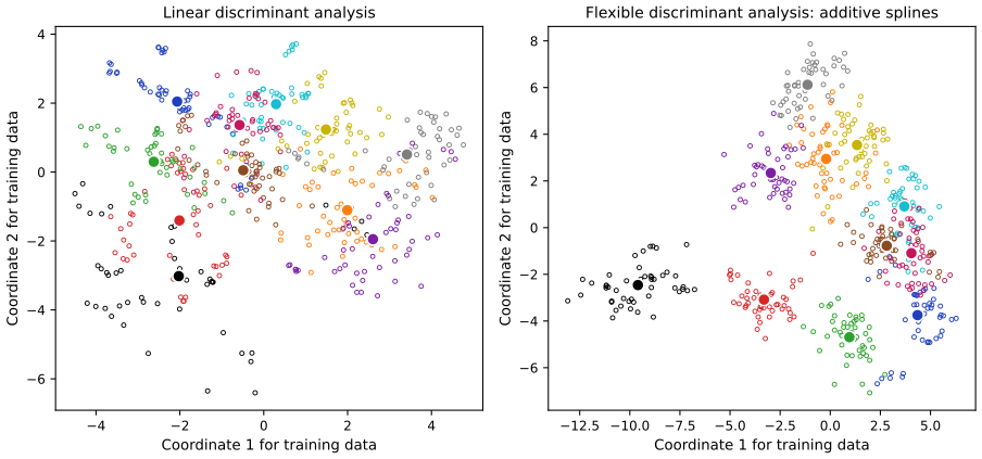
fig_12_10, vowel_fda. Reproduces Hastie, Tibshirani and Friedman (2009), Figure 12.10. Download: PDF · SVGTable 12.3. Vowel recognition: training and test error rates p. 444
| technique | train (ours) | test (ours) | train (book) | test (book) |
|---|---|---|---|---|
| LDA | 0.316 | 0.556 | 0.32 | 0.56 |
| QDA | 0.011 | 0.528 | 0.01 | 0.53 |
| FDA / additive splines, 4 df (book: BRUTO) | 0.062 | 0.457 | 0.06 | 0.44 |
| FDA / MARS (degree 1) | 0.083 | 0.461 | 0.09 | 0.45 |
| best reduced dimension (ours 4, book 2) | 0.144 | 0.426 | 0.18 | 0.42 |
| FDA / MARS (degree 2) | 0.062 | 0.455 | 0.02 | 0.42 |
| best reduced dimension (ours 8, book 6) | 0.068 | 0.448 | 0.13 | 0.39 |
The book's table also lists softmax versions, CART, neural networks and nearest neighbours (test errors 0.44–0.67), which are not fitted here. LDA and QDA agree with the book to the printed digits. Our MARS is a compact implementation (20 knots per input, GCV pruning; MARS), so its rows differ in detail; FDA with flexible regressions improves on LDA by 10–13 points of test error in both, and the reduced dimension is chosen on the test data, as in the book (vowel_table).
12.5.1 Computing the FDA Estimates
pp. 444–445 When the regression is a linear operator \(\bS_\lambda\) (\(\hat\by=\bS_\lambda\by\); additive splines with fixed smoothing parameters, MARS once its basis is chosen, any penalised basis regression), optimal scoring is a canonical correlation problem solved by one eigen-decomposition. Let \(\bY\) be the \(N\times K\) indicator matrix, \(y_{ik}=1\) if \(g_i=k\).
Definition 12.2 (the FDA computation) p. 445
- Multivariate regression. Fit a multi-response (adaptive, nonparametric) regression of \(\bY\) on \(X\), giving \(\hat\bY=\bS_\lambda\bY\) and the vector of fitted functions \(\eta^*(x)\).
- Optimal scores. Compute the eigen-decomposition of \(\bY^\T\hat\bY=\bY^\T\bS_\lambda\bY\), with eigenvectors \(\bTh\) normalised by \(\bTh^\T\Dpi\bTh=\bI\), \(\Dpi=\bY^\T\bY/N\).
- Update. \(\eta(x)=\bTh^\T\eta^*(x)\). The first of the \(K\) functions is the constant (a trivial solution); the remaining \(K-1\) are the discriminant functions, automatically centred.
Result 12.14 (why the eigen-decomposition solves optimal scoring; Exercise 12.6) p. 445
For a regression on a basis \(\bH\) (containing the constant) with projection \(\bS\), the scores minimising (12.53) under \(\bTh^\T\Dpi\bTh=\bI\) are the generalised eigenvectors of \(\bY^\T\bS\bY/N\) relative to \(\Dpi\). All eigenvalues lie in \([0,1]\), the largest is 1 with the constant eigenvector, and the residual of score \(\ell\) is \(r^2_\ell=1-\alpha^2_\ell\). For a penalised regression, \(\bS\) is replaced by \(\bS_\lambda=\bH(\bH^\T\bH+\lambda\bOm)^{-1}\bH^\T\) and \(r^2_\ell\) by the penalised criterion.
Proof
For fixed \(\theta\) the best coefficients are \(\hat\beta=(\bH^\T\bH)^{-1}\bH^\T\bY\theta\), with residual sum of squares \(\theta^\T\bY^\T(\bI-\bS)\bY\theta=N\theta^\T\Dpi\theta-\theta^\T\bY^\T\bS\bY\theta\). With \(\theta^\T\Dpi\theta=1\) this is minimised by maximising \(\theta^\T(\bY^\T\bS\bY/N)\theta\): a generalised Rayleigh quotient, maximised over \(\Dpi\)-orthonormal sets by the leading generalised eigenvectors. Since \(\bS\) is a projection, \(\theta^\T\bY^\T\bS\bY\theta=\|\bS\bY\theta\|^2\le\|\bY\theta\|^2=N\theta^\T\Dpi\theta\), so every eigenvalue is at most 1, and nonnegative. If the constant is in the span of \(\bH\), \(\bS\bone=\bone\) and \(\bY\bone=\bone\), so \(\bY^\T\bS\bY\bone=\bY^\T\bone=N\Dpi\bone\): eigenvalue 1 with \(\theta=\bone\). Every other eigenvector is \(\Dpi\)-orthogonal to \(\bone\), which is the mean-zero condition \(\sum_i\theta(g_i)=0\): the constraints of (12.52) are built in. With a penalty the same argument holds with the penalised residual \(\theta^\T\bY^\T(\bI-\bS_\lambda)\bY\theta\) (the minimum of \(\|\bY\theta-\bH\beta\|^2+\lambda\beta^\T\bOm\beta\)), and \(\bS_\lambda\preceq\bI\) when \(\bOm\succeq0\). ∎
The modularity is the point: any regression method that handles several responses at once can be plugged into step 1, and step 2 computes all the scorings together. In Section 4.2 linear regression on the indicator matrix suffered from masking with three or more classes; FDA uses the same fits but transforms them into discriminant functions that do not mask (see Exercise 12.9).
12.6 Penalized Discriminant Analysis
pp. 446–449 Suppose the FDA regression is linear in a basis expansion \(h(X)\) with a quadratic penalty:
\[ \ASR\big(\{\theta_\ell,\beta_\ell\}_{\ell=1}^L\big)=\frac1N\sum_{\ell=1}^L\Big[\sum_{i=1}^N\big(\theta_\ell(g_i)-h^\T(x_i)\beta_\ell\big)^2+\lambda\beta_\ell^\T\bOm\beta_\ell\Big]. \tag{12.57} \]\(\bOm\) depends on the problem: for spline bases it makes \(\eta_\ell\) smooth over \(\R^p\); for additive splines (\(N\) basis functions per coordinate, \(Np\) in all) it is \(Np\times Np\) and block diagonal. FDA is then a penalised LDA (PDA): enlarge the predictors to \(h(X)\); use LDA in the enlarged space with the penalised Mahalanobis distance
\[ D(x,\mu)=(h(x)-h(\mu))^\T(\SW+\lambda\bOm)^{-1}(h(x)-h(\mu)), \tag{12.58} \]\(\SW\) the within-class covariance of the \(h(x_i)\); and find the discriminant subspace with the penalised metric, \(\max u^\T\bm\Sigma_{\mathrm{Bet}}u\) subject to \(u^\T(\SW+\lambda\bOm)u=1\).
Result 12.15 (penalised optimal scoring is LDA in a penalised metric; Exercise 12.7) pp. 446–447
Let the basis be centred and the constant unpenalised, and put \(\bOm_\lambda=\lambda\bOm/N\). The minimisers of (12.57) have scores that are generalised eigenvectors of \(\bY^\T\bS_\lambda\bY/N\) relative to \(\Dpi\) (eigenvalues \(\alpha^2_\ell\)) and coefficients \(\beta_\ell=(\ST+\bOm_\lambda)^{-1}\bM^\T\Dpi\theta_\ell\) satisfying
\[ \SB\beta_\ell=\frac{\alpha^2_\ell}{1-\alpha^2_\ell}(\SW+\bOm_\lambda)\beta_\ell,\qquad\beta_\ell^\T(\SW+\bOm_\lambda)\beta_\ell=r^2_\ell(1-r^2_\ell), \]so (12.54)–(12.55) hold with the penalised Mahalanobis distance (12.58), in which \(\lambda\bOm\) is to be read as \(\lambda\bOm/N\) when \(\SW\) has divisor \(N\).
Proof
For fixed \(\theta\), (12.57) is a ridge-type regression with solution
\[ \beta=(\bH^\T\bH+\lambda\bOm)^{-1}\bH^\T\bY\theta=(\ST+\bOm_\lambda)^{-1}\bM^\T\Dpi\theta \](centred \(\bH\), mean-zero scores) and minimum \(\tfrac1N\theta^\T\bY^\T(\bI-\bS_\lambda)\bY\theta\). Result 12.14 gives the scores. The proof of Result 12.12 goes through with \(\ST\) replaced by \(\ST+\bOm_\lambda\) everywhere:
\[ \SB\beta=\alpha^2(\ST+\bOm_\lambda)\beta=\alpha^2(\SW+\bOm_\lambda+\SB)\beta \], hence the eigen-equation; \(\beta^\T(\ST+\bOm_\lambda)\beta=\alpha^2\) and \(\beta^\T\SB\beta=\alpha^4\) give the normalisation. Then the proof of Result 12.13 with \(\SW\) replaced by \(\SW+\bOm_\lambda\) gives the distances. On the vowel data with \(\bOm=\bI\) and \(\lambda=50\), the distances from the penalised fits match \((x-\mu_k)^\T(\SW+\lambda\bI/N)^{-1}(x-\mu_k)\) up to a class-free term, to \(2\times10^{-13}\). ∎
The penalised distance gives less weight to rough coordinates and more to smooth ones, and since \(\bOm\) is not diagonal the same applies to rough or smooth linear combinations. For some problems the expansion is unnecessary because there are already too many correlated predictors: the log-periodogram of speech sampled at 256 frequencies (Figure 5.5), or the 256 grey levels of a digitised digit. Neighbouring pixels are strongly positively correlated, so LDA can give them large coefficients of opposite sign that cancel on similar pixels; positively correlated predictors produce noisy, negatively correlated coefficient estimates. PDA regularises the coefficients to be smooth as an image: here \(h(X)=X\) and \(\beta^\T\bOm\beta\) penalises the roughness of \(\beta\) seen as a \(16\times16\) image.
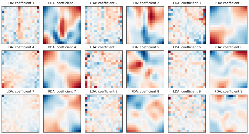
fig_12_11, image_penalty. Reproduces Hastie, Tibshirani and Friedman (2009), Figure 12.11. Download: PDF · SVG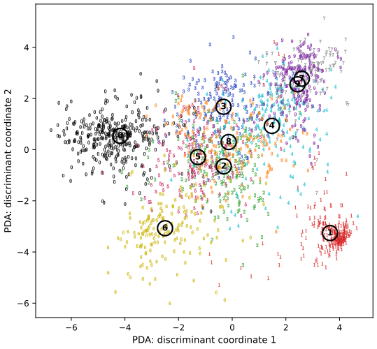
fig_12_12. Reproduces Hastie, Tibshirani and Friedman (2009), Figure 12.12. Download: PDF · SVGThe book quotes Hastie, Buja and Tibshirani (1995): regularisation improved LDA's test error by about 25% in the cases they tried. On these digits, with 7291 training images for 256 pixels, the gain we find is small: over \(\lambda\) from 30 to 3000 the PDA test error stays between 0.111 and 0.113 against LDA's 0.115 (zip_pda_errors); the smoothness buys interpretability more than accuracy here. With fewer training images per pixel, the variance reduction would matter more.
12.7 Mixture Discriminant Analysis
pp. 449–451 LDA is a prototype classifier with one prototype per class. When a class is inhomogeneous, a mixture is more appropriate. A Gaussian mixture for class \(k\) is
\[ P(X\given G=k)=\sum_{r=1}^{R_k}\pi_{kr}\phi(X;\mu_{kr},\bSig), \tag{12.59} \]with mixing proportions summing to one, \(R_k\) prototypes, and the same covariance \(\bSig\) as the metric throughout. With class priors \(\Pi_k\) the posterior is
\[ P(G=k\given X=x)=\frac{\sum_{r=1}^{R_k}\pi_{kr}\phi(x;\mu_{kr},\bSig)\Pi_k}{\sum_{\ell=1}^K\sum_{r=1}^{R_\ell}\pi_{\ell r}\phi(x;\mu_{\ell r},\bSig)\Pi_\ell}. \tag{12.60} \]The parameters are estimated by maximum likelihood with the joint log-likelihood based on \(P(G,X)\):
\[ \sum_{k=1}^K\sum_{g_i=k}\log\Big[\sum_{r=1}^{R_k}\pi_{kr}\phi(x_i;\mu_{kr},\bSig)\Pi_k\Big]. \tag{12.61} \]The sum inside the logarithm makes direct maximisation messy; EM (Dempster, Laird and Rubin, 1977; Chapter 8) is the natural algorithm. Its E-step computes the responsibility of subclass \(c_{kr}\) for each class-\(k\) observation,
\[ W(c_{kr}\given x_i,g_i)=\frac{\pi_{kr}\phi(x_i;\mu_{kr},\bSig)}{\sum_{\ell=1}^{R_k}\pi_{k\ell}\phi(x_i;\mu_{k\ell},\bSig)}, \tag{12.62} \]and its M-step computes weighted maximum likelihood estimates with these weights.
See also (companion course): Section 9.2.2, EM for Gaussian mixtures, and Section 9.4 for the general argument.
Result 12.16 (EM for MDA: the M-step is a weighted LDA) pp. 449–450
Given the responsibilities \(W_{ir}=W(c_{kr}\given x_i,g_i)\) (zero unless \(g_i=k\)), the M-step is
\[ \hat\pi_{kr}=\frac{\sum_{g_i=k}W_{ir}}{N_k},\qquad\hat\mu_{kr}=\frac{\sum_iW_{ir}x_i}{\sum_iW_{ir}},\qquad\hat{\bSig}=\frac1N\sum_{i=1}^N\sum_{r}W_{ir}(x_i-\hat\mu_{kr})(x_i-\hat\mu_{kr})^\T,\qquad\hat\Pi_k=\frac{N_k}{N}: \]LDA with the \(R=\sum_kR_k\) subclasses as classes and observation \(i\) counted in subclass \(r\) with weight \(W_{ir}\). Each EM step does not decrease (12.61).
Proof
EM maximises, at each M-step, the expected complete-data log-likelihood
\[ \sum_i\sum_rW_{ir}[\log\pi_{kr}+\log\phi(x_i;\mu_{kr},\bSig)]+\sum_i\log\Pi_{g_i} \], the expectation of the log-likelihood that would apply if the subclass of each observation were known. It separates. Proportions: maximise \(\sum_rn_{kr}\log\pi_{kr}\) with \(n_{kr}=\sum_iW_{ir}\) subject to \(\sum_r\pi_{kr}=1\); a Lagrange multiplier gives \(\pi_{kr}\propto n_{kr}\), and \(\sum_rn_{kr}=N_k\) because each class-\(k\) row of \(W\) sums to one. Means: the gradient in \(\mu_{kr}\) is \(\bSig^{-1}\sum_iW_{ir}(x_i-\mu_{kr})\), zero at the weighted mean. Covariance: with \(\bm P=\bSig^{-1}\) the terms are \(\tfrac N2\log\det\bm P-\tfrac12\Tr(\bm P\bm A)\) with \(\bm A=\sum_i\sum_rW_{ir}(x_i-\mu_{kr})(x_i-\mu_{kr})^\T\); the derivative \(\tfrac N2\bm P^{-1}-\tfrac12\bm A\) vanishes at \(\bSig=\bm A/N\). Priors: the class labels are observed, so \(\hat\Pi_k=N_k/N\). These are the estimates of LDA (Section 4.3) for \(R\) classes with weighted observations. That the observed log-likelihood never decreases is the general EM property: (12.61) minus the expected complete-data log-likelihood is a sum of entropy terms maximised at the current responsibilities (companion course, Section 9.4). Numerically the log-likelihood increased at every one of the 41 iterations of the fit in Figure 12.13. ∎
In the E-step the unit weight of each observation is shared among its own class's subclasses: a point near one subclass centroid and far from the others gets weight near one there; a point halfway between two gets about half each. In the M-step a class-\(k\) observation is used \(R_k\) times, with different weights. Mixture likelihoods are multimodal, so the start matters; the default of the book's software is a \(k\)-means clustering with several random starts within each class, whose partition gives an initial 0/1 weight matrix.
The common covariance buys more. The rank-\(L\) LDA fit is the maximum-likelihood fit of a Gaussian model whose class means lie in a rank-\(L\) subspace (Exercise 4.8, Result 4.7), and MDA inherits this: maximise (12.61) subject to \(\rank\{\mu_{k\ell}\}=L\). EM still works, and its M-step becomes a weighted rank-\(L\) LDA with \(R\) classes, which can be computed by optimal scoring and hence replaced by a weighted FDA or PDA. One might expect the number of observations to grow by the factor \(R_k\) as well, but for linear regression operators it does not: the expanded indicator matrix collapses into a blurred response matrix \(\bZ\) (\(N\times R\)) whose class-\(k\) rows hold the responsibilities \(W(c_{kr}\given x_i,g_i)\), for example, with \(K=3\) and \(R_k=3\),
\[ \bZ=\begin{pmatrix}&c_{11}&c_{12}&c_{13}&c_{21}&c_{22}&c_{23}&c_{31}&c_{32}&c_{33}\\ g_1=2&0&0&0&0.3&0.5&0.2&0&0&0\\ g_2=1&0.9&0.1&0.0&0&0&0&0&0&0\\ g_3=1&0.1&0.8&0.1&0&0&0&0&0&0\\ g_4=3&0&0&0&0&0&0&0.5&0.4&0.1\\ \vdots&&&&&\vdots&&&&\\ g_N=3&0&0&0&0&0&0&0.1&0.1&0.8\end{pmatrix}, \tag{12.63} \]and the remaining steps are the same: \(\hat\bZ=\bS\bZ\), \(\bZ^\T\hat\bZ=\bTh\bm D\bTh^\T\), update the \(\pi\)'s and \(\Pi\)'s.
Filling the gap 12.8: why the expanded indicator matrix collapses to \(\bZ\) p. 450
Derivation
The weighted LDA of the M-step has, for each observation \(i\) of class \(k\), \(R_k\) copies \((h(x_i),e_{kr})\) with weights \(W_{ir}\), where \(e_{kr}\) is the indicator of subclass \(kr\). Stack them in \(\bH_{\rm big}\), \(\bY_{\rm big}\) and the diagonal weight matrix \(\bm\Lambda\). The weighted (penalised) regression of \(\bY_{\rm big}\) on \(\bH_{\rm big}\) has normal equations with
\[ \bH_{\rm big}^\T\bm\Lambda\bH_{\rm big}=\sum_i\Big(\sum_rW_{ir}\Big)h(x_i)h(x_i)^\T=\bH^\T\bH,\qquad\bH_{\rm big}^\T\bm\Lambda\bY_{\rm big}=\sum_ih(x_i)\Big(\sum_rW_{ir}e_{kr}\Big)^\T=\bH^\T\bZ, \]because each row of \(W\) sums to one. So the coefficient matrix is that of the ordinary regression of \(\bZ\) on \(\bH\). The optimal-scoring matrix is \(\bY_{\rm big}^\T\bm\Lambda\hat\bY_{\rm big}=\bZ^\T\bH\hat\bB=\bZ^\T\hat\bZ\), and the normalising matrix is \(\bY_{\rm big}^\T\bm\Lambda\bY_{\rm big}=\diag(\bZ^\T\bone)\) (the subclass totals), not \(\bZ^\T\bZ\). Nothing of size \(N\sum R_k\) is ever formed. Running EM with this M-step (MDAScoring) and with the direct Gaussian M-step of Result 12.16 (MDAGauss) from the same start gives the same responsibilities after 10 iterations to \(3\times10^{-14}\). ∎
These modifications add a lot of flexibility. The dimension reduction of LDA, FDA or PDA is limited by the number of classes (none at all for \(K=2\)); MDA substitutes subclasses for classes and allows low-dimensional views of the subspace spanned by the subclass centroids, often an important one for discrimination. And using FDA or PDA in the M-step adapts MDA further, for example with smoothness constraints for signals and images.
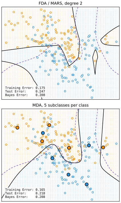
fig_12_13. Reproduces Hastie, Tibshirani and Friedman (2009), Figure 12.13. Download: PDF · SVG12.7.1 Example: Waveform Data
pp. 451–454 A three-class simulated problem in 21 dimensions from Breiman, Friedman, Olshen and Stone (1984), considered difficult:
\[ \begin{aligned}X_j&=Uh_1(j)+(1-U)h_2(j)+\epsilon_j&&\text{Class 1},\\ X_j&=Uh_1(j)+(1-U)h_3(j)+\epsilon_j&&\text{Class 2},\\ X_j&=Uh_2(j)+(1-U)h_3(j)+\epsilon_j&&\text{Class 3},\end{aligned} \tag{12.64} \]\(j=1,\dots,21\), \(U\sim U(0,1)\), \(\epsilon_j\) standard normal, with the shifted triangles \(h_1(j)=\max(6-|j-11|,0)\), \(h_2(j)=h_1(j-4)\) and \(h_3(j)=h_1(j+4)\).
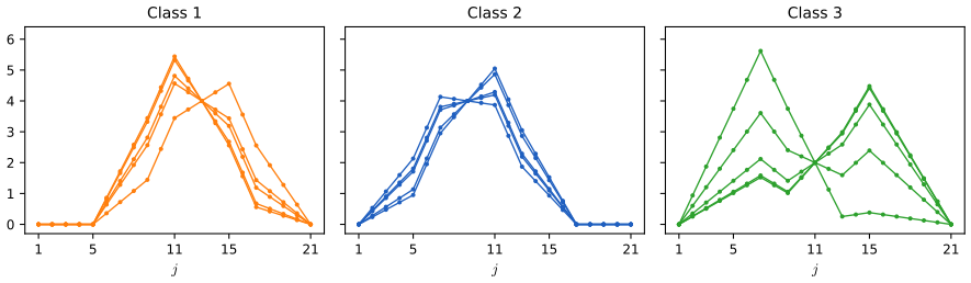
fig_12_14. Reproduces Hastie, Tibshirani and Friedman (2009), Figure 12.14. Download: PDF · SVGTraining samples have 300 observations with equal priors (about 100 per class) and test samples 500. The Bayes risk is about 0.14 (Breiman et al., 1984).
Table 12.4. Waveform data: error rates, averages over ten simulations (standard errors) p. 454
| technique | train (ours) | test (ours) | train (book) | test (book) |
|---|---|---|---|---|
| LDA | 0.132 (0.008) | 0.197 (0.006) | 0.121 (0.006) | 0.191 (0.006) |
| QDA | 0.040 (0.003) | 0.209 (0.006) | 0.039 (0.004) | 0.205 (0.006) |
| CART | 0.117 (0.015) | 0.290 (0.007) | 0.072 (0.003) | 0.289 (0.004) |
| FDA/MARS (degree 1) | 0.130 (0.007) | 0.196 (0.008) | 0.100 (0.006) | 0.191 (0.006) |
| FDA/MARS (degree 2) | 0.129 (0.008) | 0.200 (0.007) | 0.068 (0.004) | 0.215 (0.002) |
| MDA (3 subclasses) | 0.090 (0.005) | 0.176 (0.005) | 0.087 (0.005) | 0.169 (0.006) |
| MDA (3 subclasses, penalised 4 df) | 0.161 (0.009) | 0.187 (0.004) | 0.137 (0.006) | 0.157 (0.005) |
| PDA (penalised 4 df) | 0.175 (0.008) | 0.187 (0.005) | 0.150 (0.005) | 0.171 (0.005) |
| MDA (3 subclasses, penalised 8 df) | 0.108 (0.006) | 0.149 (0.006) | ||
| PDA (penalised 8 df) | 0.135 (0.006) | 0.158 (0.006) | ||
| Bayes | 0.140 | 0.140 |
The first five rows of the book's table come from Hastie, Tibshirani and Buja (1994). The penalty is the second-difference roughness of the coefficients in \(j\). The book does not say how "4 df" is measured; we take \(\lambda\) with \(\Tr[\bX_c(\bX_c^\T\bX_c+\lambda\bOm)^{-1}\bX_c^\T]=4\), which turns out to penalise more than the book's fits (their training errors 0.137 and 0.150 lie between our 4 df and 8 df rows), so we add the 8 df rows. With that, penalised MDA reaches 0.149, close to the Bayes rate. CART is pruned by 10-fold cross-validation (waveform_table).
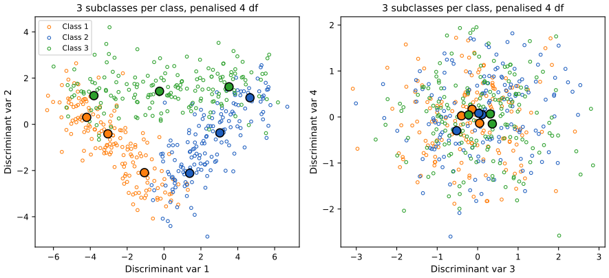
fig_12_15. Reproduces Hastie, Tibshirani and Friedman (2009), Figure 12.15. Download: PDF · SVGFilling the gap 12.9: why a triangle, and why two dimensions suffice p. 453
Derivation
Without noise, a class-1 waveform is \(Uh_1+(1-U)h_2\), a point on the segment from \(h_2\) to \(h_1\) in \(\R^{21}\); classes 2 and 3 lie on the segments \([h_3,h_1]\) and \([h_3,h_2]\). The three vectors \(h_1,h_2,h_3\) are the vertices of a triangle, and the three classes live on its three edges, all inside the two-dimensional affine plane through the vertices. The noise \(\epsilon\sim N(0,\bI)\) is isotropic, so the within-class covariance of class \((a,b)\) is \(\bI+\Var(U)(h_a-h_b)(h_a-h_b)^\T\). Every subclass centroid (the mean of \(X\) over a range of \(U\)) is a convex combination of two vertices, so in the population all nine subclass centroids lie in the plane and the between-subclass covariance has rank 2; with the common covariance as metric only two discriminant coordinates carry signal, and in them the data form the triangle's edges. In a sample the other eigenvalues are small but not zero (the third and fourth are 0.064 and 0.015 against 8.71 and 1.96 in the fit of Figure 12.15). MDA's structure matches the generating model (each class a continuum of Gaussians along a segment, approximated by three), which is why it comes close to the Bayes rate. ∎
Computational Considerations
p. 455 With \(N\) training cases, \(p\) predictors and \(m\) support vectors, the SVM needs about \(m^3+mN+mpN\) operations (taking \(m\approx N\)), so it does not scale well with \(N\); decomposition methods such as SMO (Platt, 1999) help. LDA and PDA need \(Np^2+p^3\) operations. FDA costs whatever its regression costs: additive models and MARS are linear in \(N\), general splines and kernel regressions typically \(N^3\). The book's software for FDA, PDA and MDA is the R package mda; the course code implements the three methods itself (OptimalScoring, MDAGauss, MDAScoring). The path algorithm of Section 12.3.5 costs about as much as a single SVM fit and gives every \(C\) at once.
Exercises
All 11 exercises of Chapter 12 (Hastie, Tibshirani and Friedman, 2009, pp. 455–458), restated in my own words, with complete solutions (hidden).
Exercise 12.1. Show that the criteria (12.25) and (12.8) are equivalent.
Solution
This is Result 12.5. In (12.8), for fixed \((\beta,\beta_0)\) the best slacks are \(\xi_i=[1-y_if(x_i)]_+\), which reduces (12.8) to
\[ \tfrac12\|\beta\|^2+C\sum_i[1-y_if(x_i)]_+=C\cdot\{\text{(12.25) with }\lambda=1/C\} \]. A positive multiple of an objective has the same minimisers, so the two problems have the same solutions \((\hat\beta,\hat\beta_0)\) whenever \(\lambda=1/C\). The multipliers correspond as \(\alpha_i^{(12.8)}=C\,\alpha_i^{(12.33)}\), which is why the path multipliers lie in \([0,1]\) and the SVM's in \([0,C]\).
Exercise 12.2. Show that the solution of (12.29) is the same as that of (12.25) for a particular kernel.
Solution
Take \(K(x,x')=h(x)^\T h(x')\), so \(\bK=\bH\bH^\T\). Any \(\beta\in\R^M\) splits as \(\beta=\bH^\T\alpha+\beta_\perp\) with \(\bH\beta_\perp=0\) (row space plus its orthogonal complement). Then \(f(x_i)=\beta_0+(\bH\beta)_i=\beta_0+(\bK\alpha)_i\) does not involve \(\beta_\perp\), while \(\|\beta\|^2=\alpha^\T\bK\alpha+\|\beta_\perp\|^2\). The minimiser of (12.25) therefore has \(\beta_\perp=0\), and (12.25) restricted to \(\beta=\bH^\T\alpha\) is exactly (12.29). Conversely a minimiser \(\hat\alpha\) of (12.29) gives the minimiser \(\hat\beta=\bH^\T\hat\alpha\) of (12.25), with the same fitted function \(\hat f(x)=\hat\beta_0+\sum_i\hat\alpha_iK(x,x_i)\) (12.28). For an infinite expansion (12.26) the same argument is the representer theorem (Result 12.7). Checked numerically: the degree-2 kernel SVM and the SVM on the explicit features (12.23) agree to \(10^{-12}\).
Exercise 12.3. Modify (12.43) so that the constant is not penalised (squared-error loss). Formulate the problem and characterise its solution.
Solution
Minimise \(\|\by-\beta_0\bone-\bH\beta\|^2+\lambda\|\beta\|^2\) over \(\beta_0\) and \(\beta\), where \(\bH\) no longer contains the constant. For fixed \(\beta_0\) this is (12.45) with response \(\by-\beta_0\bone\), so by Result 12.10 \(\hat\beta=\bH^\T\hat\alpha\) with \(\hat\alpha=(\bK+\lambda\bI)^{-1}(\by-\beta_0\bone)\), \(\bK=\bH\bH^\T\). The derivative in \(\beta_0\) gives \(\bone^\T(\by-\beta_0\bone-\bK\hat\alpha)=0\); since \(\by-\beta_0\bone-\bK\hat\alpha=\lambda\hat\alpha\), this is \(\bone^\T\hat\alpha=0\). Writing \(\bm A=\bK+\lambda\bI\) (positive definite),
\[ \hat\beta_0=\frac{\bone^\T\bm A^{-1}\by}{\bone^\T\bm A^{-1}\bone},\qquad\hat\alpha=\bm A^{-1}(\by-\hat\beta_0\bone),\qquad\hat f(x)=\hat\beta_0+\sum_{i=1}^N\hat\alpha_iK(x,x_i). \]So the solution again needs only the kernel; \(\hat\beta_0\) is a generalised-least-squares mean of \(\by\) with weight matrix \(\bm A^{-1}\), and the coefficients sum to zero. Equivalently, \(\hat\beta_0\) and \(\hat\alpha\) solve the bordered system \(\begin{pmatrix}\bm A&\bone\\\bone^\T&0\end{pmatrix}\begin{pmatrix}\hat\alpha\\\hat\beta_0\end{pmatrix}=\begin{pmatrix}\by\\0\end{pmatrix}\), the same structure as the SVM's \(\sum\alpha_iy_i=0\). The formula agrees with a direct primal solve to \(10^{-9}\) (
kernel_ridge_with_intercept).Exercise 12.4. In reduced-rank LDA for \(K\) groups, let \(z=\bU^\T x\) be the canonical variables, \(\bU\) the \(p\times L\) matrix of discriminant coefficients (\(L\le K-1\), \(p>K\)). (a) If \(L=K-1\), show that
\[ \|z-\bar z_k\|^2-\|z-\bar z_{k'}\|^2=\|x-\bar x_k\|^2_W-\|x-\bar x_{k'}\|^2_W \], the difference of Mahalanobis distances with respect to the within covariance \(\bW\). (b) If \(L\lt K-1\), show that the left side measures the difference of Mahalanobis distances for the distributions projected onto the subspace spanned by \(\bU\).
Solution
Normalise the discriminant directions as LDA does, \(\bU^\T\bW\bU=\bI\), and complete them to \(\nu_1,\dots,\nu_p\) with \(\bm V^\T\bW\bm V=\bI\), so \(\bW^{-1}=\bm V\bm V^\T\) and \(\|x-\bar x_k\|^2_W=\sum_{\ell=1}^p(\nu_\ell^\T(x-\bar x_k))^2\).
(a) As in the proof of Result 12.13, for \(\ell\ge K\) the term \(\nu_\ell^\T\bar x_k\) is the same for all \(k\), so
\[ \|x-\bar x_k\|^2_W=\|\bU^\T(x-\bar x_k)\|^2+D(x)=\|z-\bar z_k\|^2+D(x) \]with \(D\) free of \(k\). Subtracting the same identity for \(k'\) cancels \(D(x)\).
(b) For \(L\lt K-1\) let \(\bm P=\bW\bU\bU^\T\). It is the projection onto \(\span(\bW\bU)\) that is orthogonal in the Mahalanobis inner product \(\langle a,b\rangle=a^\T\bW^{-1}b\): \(\bm P^2=\bW\bU(\bU^\T\bW\bU)\bU^\T=\bm P\) and \(\bW^{-1}\bm P=\bU\bU^\T\) is symmetric. Then
\[ \|\bm P(x-\bar x_k)\|^2_W=(x-\bar x_k)^\T\bU\bU^\T\bW\bW^{-1}\bW\bU\bU^\T(x-\bar x_k)=\|\bU^\T(x-\bar x_k)\|^2=\|z-\bar z_k\|^2. \]So \(\|z-\bar z_k\|^2\) is the Mahalanobis distance between the projections of \(x\) and \(\bar x_k\) on the subspace \(\span(\bW\bU)\), which is the span of the leading \(L\) directions of between-class variation (\(\bW\nu_\ell\propto\SB\nu_\ell\)); the left side of (a) is the difference of these projected distances. Both identities hold to \(10^{-8}\) on the vowel data.
Exercise 12.5. The phoneme data consist of log-periodograms at 256 frequencies for five phoneme classes. (a) Plot the curves against frequency for each class. (b) To classify by nearest prototype, fit \(K\)-means in each class and classify to the class of the closest centre, but restrict each prototype to be smooth, \(m=\bB\theta\) with \(\bB\) a \(256\times J\) natural-spline basis with \(J\) knots equally spaced over \((0,255)\). Describe how to proceed analytically and how to avoid high-dimensional fitting (hint: make \(\bB\) orthogonal). (c) Implement it with a 50-50 split that keeps each speaker in one half (why?), \(K=1,3,5,7\) centres per class and \(J=5,10,15\), with the same \(K\)-means starts for every \(J\); compare.
Solution
(a) The curves (plots of the same kind as Figure 5.5 for "aa" and "ao") show a strong common shape per class with large frame-to-frame noise at high frequencies; the classes differ mainly at low frequencies.
(b) Orthonormalise the basis, \(\bB=\bm Q\bm R\) by QR, and reparametrise \(m=\bm Q\vartheta\) (\(\vartheta=\bm R\theta\)); the set of smooth prototypes is unchanged. With \(\bm Q^\T\bm Q=\bI\), Pythagoras gives, for every curve \(x\in\R^{256}\),
\[ \|x-\bm Q\vartheta\|^2=\|x-\bm Q\bm Q^\T x\|^2+\|\bm Q^\T x-\vartheta\|^2. \]The first term does not depend on the prototype. So (i) \(K\)-means with smooth prototypes on the curves is ordinary \(K\)-means on the \(J\)-dimensional coordinates \(z=\bm Q^\T x\), the centre update being the mean of the \(z\)'s (the least-squares smooth of the mean curve); and (ii) the closest smooth prototype to a test curve is the closest \(\vartheta\) to its \(z\). One projection of the data (\(N\times256\) times \(256\times J\)) replaces all 256-dimensional computations.
(c) Frames from the same speaker are strongly correlated (same voice, same recording). With a speaker in both halves, the test frames would have near-duplicates in the training set and the test error would be optimistic for new speakers. We split the 437 speaker identifiers of
phoneme.dataat random into halves (phoneme_split, seed 5), drew five sets of starting rows per class and \(K\), and used them for every \(J\) (exercise_12_5). Test error rates (\(J=256\): unrestricted prototypes):centres per class \(J=5\) \(J=10\) \(J=15\) unrestricted \(K=1\) 0.168 0.122 0.121 0.119 \(K=3\) 0.151 0.109 0.106 0.105 \(K=5\) 0.153 0.112 0.109 0.101 \(K=7\) 0.146 0.111 0.105 0.094 Five knots are too few (the prototypes miss real spectral structure); with 10–15 knots the smooth prototypes are within about one point of the unrestricted ones, at a fraction of the dimension. Several prototypes per class help (the error falls from 0.12 to about 0.105 with three). With roughly 2,250 training curves the unrestricted means are already precise, so smoothing does not lower the error here; its value is in stability and interpretability when the sample is small relative to 256.
Exercise 12.6. Let the FDA regression be a linear expansion in basis functions \(h_m(x)\), \(m=1,\dots,M\), and \(\Dpi=\bY^\T\bY/N\). (a) Show that (12.52) can be written \(\min_{\theta,\beta}\|\bY\theta-\bH\beta\|^2\) (12.65), \(\bH\) the \(N\times M\) matrix of \(h_j(x_i)\). (b) Interpret the normalisations \(\theta^\T\Dpi\bone=0\), \(\theta^\T\Dpi\theta=1\). (c) Show that minimising over \(\beta\) leads to \(\max_\theta\theta^\T\bS\theta\) (12.66) under these constraints, \(\bS\) the projection of \(\bH\). (d) If the \(h_j\) include the constant, show that the largest eigenvalue is 1. (e) With \(\bTh\) (\(K\times K\)) normalised by \(\bTh^\T\Dpi\bTh=\bI\), show that the solution of (12.53) is the complete set of eigenvectors; the first is trivial and handles the centring, the rest are the optimal scores.
Solution
(a) The \(i\)-th entry of \(\bY\theta\) is \(\theta(g_i)\) (row \(i\) of \(\bY\) is the indicator of \(g_i\)) and that of \(\bH\beta\) is \(h(x_i)^\T\beta\); the sum of squares in (12.52) is \(\|\bY\theta-\bH\beta\|^2\).
(b) \(\theta^\T\Dpi\bone=\frac1N\sum_k N_k\theta_k=\frac1N\sum_i\theta(g_i)=0\): the scored labels have mean zero over the training data. \(\theta^\T\Dpi\theta=\frac1N\sum_i\theta(g_i)^2=1\): with mean zero, unit variance. Together they rule out the trivial \(\theta=0\) (or constant \(\theta\), fitted perfectly by the constant).
(c) For fixed \(\theta\), \(\hat\beta=(\bH^\T\bH)^{-1}\bH^\T\bY\theta\) and, under \(\theta^\T\Dpi\theta=1\),
\[ \|\bY\theta-\bS\bY\theta\|^2=\theta^\T\bY^\T(\bI-\bS)\bY\theta=N-\theta^\T\bY^\T\bS\bY\theta. \]So the problem is \(\max_\theta\theta^\T(\bY^\T\bS\bY)\theta\) subject to the constraints; (12.66)'s "\(\theta^\T\bS\theta\)" is to be read as this \(K\times K\) quadratic form.
(d) \(\bS\) itself is a projection, with eigenvalues 0 and 1. For the relevant generalised problem \(\bY^\T\bS\bY\theta=\alpha^2N\Dpi\theta\): \(\alpha^2\le1\) because \(\|\bS\bY\theta\|\le\|\bY\theta\|\), and \(\theta=\bone\) attains 1 because \(\bS\bone=\bone\) when the constant is in the basis (Result 12.14).
(e) (12.53) with \(L=K\) scores is \(\min\Tr[(\bY\bTh-\bH\bB)^\T(\bY\bTh-\bH\bB)]/N\); minimising over \(\bB\) leaves \(K-\Tr(\bTh^\T\bY^\T\bS\bY\bTh)/N\), and maximising \(\Tr(\bTh^\T\bm A\bTh)\) subject to \(\bTh^\T\Dpi\bTh=\bI\) is solved by the generalised eigenvectors of \(\bm A=\bY^\T\bS\bY/N\) relative to \(\Dpi\) (substitute \(\bTh=\Dpi^{-1/2}\bm V\) to reduce to an ordinary symmetric eigenproblem and use Ky Fan's theorem). The first eigenvector is \(\bone\) with eigenvalue 1; \(\Dpi\)-orthogonality to it is the centring \(\theta^\T\Dpi\bone=0\), so the remaining \(K-1\) are exactly the constrained optimal scores. (The book's "eigenvectors of \(\bS\)" should be read as eigenvectors of \(\bY^\T\bS\bY\) relative to \(\Dpi\).) On the vowel data the leading eigenvalue is 1 to \(10^{-12}\).
Exercise 12.7. Derive the solution of the penalised optimal scoring problem (12.57).
Solution
For fixed \(\theta\) the minimiser of \(\|\bY\theta-\bH\beta\|^2+\lambda\beta^\T\bOm\beta\) is \(\hat\beta=(\bH^\T\bH+\lambda\bOm)^{-1}\bH^\T\bY\theta\), with minimum \(\theta^\T\bY^\T(\bI-\bS_\lambda)\bY\theta\), \(\bS_\lambda=\bH(\bH^\T\bH+\lambda\bOm)^{-1}\bH^\T\) (expand and use the normal equations: the minimum of \(\|\by-\bH\beta\|^2+\lambda\beta^\T\bOm\beta\) is \(\by^\T\by-\by^\T\bH\hat\beta\)). With \(\theta^\T\Dpi\theta=1\), (12.57) becomes \(\max\theta^\T(\bY^\T\bS_\lambda\bY/N)\theta\): the scores are the leading generalised eigenvectors of \(\bY^\T\bS_\lambda\bY/N\) relative to \(\Dpi\) (Steps 1–3 of Definition 12.2 with \(\bS_\lambda\)), the coefficients are \(\hat\beta_\ell=(\bH^\T\bH+\lambda\bOm)^{-1}\bH^\T\bY\theta_\ell\), and each score's penalised criterion equals \(1-\alpha^2_\ell\) (checked to \(10^{-10}\)). Result 12.15 shows that this is LDA in the metric \(\SW+\lambda\bOm/N\), i.e. the penalised LDA (12.58).
Exercise 12.8. Show that the coefficients \(\beta_\ell\) found by optimal scoring are proportional to the discriminant directions \(\nu_\ell\) of LDA.
Solution
This is Result 12.12: with \(\beta_\ell=\ST^{-1}\bM^\T\Dpi\theta_\ell\), the eigen-equation for the scores gives \(\SB\beta_\ell=\alpha^2_\ell\ST\beta_\ell\), hence \(\SB\beta_\ell=\frac{\alpha_\ell^2}{1-\alpha_\ell^2}\SW\beta_\ell\), the generalised eigen-equation of the discriminant directions; and \(\beta_\ell^\T\SW\beta_\ell=r^2_\ell(1-r^2_\ell)\), so \(\beta_\ell=\sqrt{r^2_\ell(1-r^2_\ell)}\,\nu_\ell\) with \(\nu_\ell^\T\SW\nu_\ell=1\). On the vowel data the constant of proportionality matches this formula to \(5\times10^{-13}\) for all ten directions.
Exercise 12.9. Let \(\hat\bY=\bX\hat\bB\) be the fitted \(N\times K\) indicator matrix from linear regression on the \(N\times p\) matrix \(\bX\) (\(p>K\)), and \(x^*_i=\hat\bB^\T x_i\). Show that LDA on the \(x^*_i\) is equivalent to LDA in the original space.
Solution
Centre \(\bX\) (the intercept handles the means). Then \(\hat\bB=\ST^{-1}\bM^\T\Dpi\), and since \(\bM^\T\Dpi\bone=\bM^\T\pi=0\) its columns are linearly dependent: \(x^*\) has rank \(K-1\) (drop one column, or use a generalised inverse). By the Woodbury identity,
\[ \ST^{-1}\bM^\T=(\SW+\bM^\T\Dpi\bM)^{-1}\bM^\T=\SW^{-1}\bM^\T(\bI+\Dpi\bM\SW^{-1}\bM^\T)^{-1} \], so \(\span(\hat\bB)=\span(\SW^{-1}\bM^\T)\), which is the span of the discriminant directions \(\nu_1,\dots,\nu_{K-1}\) (each \(\nu_\ell=\SW^{-1}\SB\nu_\ell/\lambda_\ell\) lies in \(\span(\SW^{-1}\bM^\T)\), and the dimensions agree). Write \(\hat\bB=\bm V_{K-1}\bm A\) with \(\bm A\) of full row rank \(K-1\). LDA on \(x^*\) uses the class means \(\hat\bB^\T\hat\mu_k\) and within covariance \(\hat\bB^\T\SW\hat\bB=\bm A^\T\bm A\), so its Mahalanobis distance is
\[ (x-\hat\mu_k)^\T\hat\bB(\bm A^\T\bm A)^{+}\hat\bB^\T(x-\hat\mu_k)=(x-\hat\mu_k)^\T\bm V_{K-1}\bm A(\bm A^\T\bm A)^+\bm A^\T\bm V_{K-1}^\T(x-\hat\mu_k)=\sum_{\ell=1}^{K-1}\big(\nu_\ell^\T(x-\hat\mu_k)\big)^2, \]because \(\bm A(\bm A^\T\bm A)^+\bm A^\T=\bI_{K-1}\). By the proof of Result 12.13 this is the original Mahalanobis distance minus a term \(D(x)\) common to all classes; the priors are the same, so the two LDA rules classify identically (confirmed on all 462 vowel test points). This is why FDA's step 2 can work on the fitted values \(\hat\bY\) alone, and why the masking of plain indicator regression (Section 4.2) disappears: LDA on the fits recovers the full LDA.
Exercise 12.10. Kernels and LDA. Carry out two-class LDA on a high-dimensional vector of transformations \(h(x)\), with the regularised within-class covariance \(\bW_h+\gamma\bI\). Show that the model can be estimated from the inner products \(K(x_i,x_{i'})=\langle h(x_i),h(x_{i'})\rangle\) alone, so that regularised LDA shares the kernel property.
Solution
Let \(\bH\) have rows \(h(x_i)^\T\), \(\bK=\bH\bH^\T\), and let \(d\in\R^N\) have entries \(1/N_+\) on class \(+1\) and \(-1/N_-\) on class \(-1\), so \(\bar h_+-\bar h_-=\bH^\T d\). The within-class covariance is \(\bW_h=\bH^\T\bm C\bH\) with \(\bm C=\frac1N\sum_k(\bI_k-\bone_k\bone_k^\T/N_k)\), the block-diagonal centring matrix (zero outside each class's block). The LDA direction solves \((\bW_h+\gamma\bI)\beta=\bH^\T d\). Rearranging, \(\gamma\beta=\bH^\T(d-\bm C\bH\beta)\), so \(\beta=\bH^\T c\) for some \(c\in\R^N\); substituting,
\[ \bH^\T\big[(\bm C\bK+\gamma\bI)c-d\big]=0,\qquad\text{which holds if}\quad(\bm C\bK+\gamma\bI)c=d. \]The matrix is invertible (\(\bm C\bK\) is similar to the positive semidefinite \(\bK^{1/2}\bm C\bK^{1/2}\) on the range of \(\bK\), so its eigenvalues are nonnegative), and the solution gives the unique \(\beta\) because \((\bW_h+\gamma\bI)\) is invertible. The discriminant function is \(h(x)^\T\beta=\sum_ic_iK(x,x_i)\); the class means of it, \(\bar s_\pm\), are averages of \((\bK c)_i\), and the rule is: class \(+1\) if
\[ \sum_ic_iK(x,x_i)>\tfrac12(\bar s_++\bar s_-)+(\text{a prior term}) \]. Only kernel values appear. With the degree-2 kernel the scores agree with the explicit six-feature computation to \(10^{-14}\) (
kernel_lda_two_class).Exercise 12.11. In MDA each mixture centre belongs to one class. A more general model (MDA2) lets every centre be shared by all classes: \(P(G,X)=\sum_{r=1}^R\pi_rP_r(G,X)\) (12.67) with \(P_r(G,X)=P_r(G)\phi(X;\mu_r,\bSig)\) (12.68), so that each region centred at \(\mu_r\) has a class profile \(P_r(G)\), and
\[ P(G=k\given X=x)=\sum_r\pi_rP_r(G=k)\phi(x;\mu_r,\bSig)/\sum_r\pi_r\phi(x;\mu_r,\bSig) \](12.69). (a) Show that MDA2 generalises MDA, with
\[ P(X\given G=k)=\sum_r\pi_rP_r(G=k)\phi(x;\mu_r,\bSig)/\sum_r\pi_rP_r(G=k) \](12.70) and mixing proportions \(\pi_{rk}=\pi_rP_r(G=k)/\sum_r\pi_rP_r(G=k)\). (b) Derive its EM algorithm. (c) Show that if the initial weights are those of MDA (separate \(k\)-means in each class), the algorithm is identical to MDA.
Solution
(a) Summing (12.67) over \(X\) gives \(P(G=k)=\sum_r\pi_rP_r(G=k)\), and \(P(X\given G=k)=P(G=k,X)/P(G=k)\) is (12.70): a Gaussian mixture with common covariance and class-specific proportions \(\pi_{rk}\), summing to one over \(r\). MDA is the special case in which each \(P_r(\cdot)\) puts all its mass on one class: then \(\pi_{rk}=0\) for centres of other classes and (12.70) is (12.59). The denominator of (12.69) is \(\sum_kP(G=k,x)=P(x)\).
(b) The latent variable is the centre \(r\) of each observation; \((g_i,x_i)\) is observed. E-step:
\[ W_{ir}=\pi_rP_r(g_i)\phi(x_i;\mu_r,\bSig)/\sum_s\pi_sP_s(g_i)\phi(x_i;\mu_s,\bSig) \]. M-step, maximising
\[ \sum_i\sum_rW_{ir}\big[\log\pi_r+\log P_r(g_i)+\log\phi(x_i;\mu_r,\bSig)\big]: \]\(\hat\pi_r=\frac1N\sum_iW_{ir}\); \(\hat P_r(k)=\sum_{g_i=k}W_{ir}/\sum_iW_{ir}\) (a weighted class histogram per centre, by the same Lagrange argument as for \(\pi\)); \(\hat\mu_r=\sum_iW_{ir}x_i/\sum_iW_{ir}\); \(\hat\bSig=\frac1N\sum_i\sum_rW_{ir}(x_i-\hat\mu_r)(x_i-\hat\mu_r)^\T\) (
mda2_em).(c) Suppose every class-\(k\) observation has weight only on the centres assigned to class \(k\). Then the M-step gives \(\hat P_r(k)=1\) for the class of centre \(r\) and 0 for the others. In the next E-step \(W_{ir}\propto\pi_rP_r(g_i)\phi(\cdot)\) is zero for centres of other classes, and for the centres of class \(g_i\) it is \(\propto\pi_r\phi(x_i;\mu_r,\bSig)\), i.e. \(\propto\pi_{kr}\phi\) with \(\pi_{kr}=\pi_r/\sum_{s\in k}\pi_s\): the MDA E-step (12.62). By induction the weights stay block-structured forever, and the M-steps coincide with Result 12.16 (\(\hat\pi_r=(N_k/N)\hat\pi_{kr}\), same means and covariance). So the two algorithms produce the same sequence of fits; on the mixture data with \(R_k=3\) the responsibilities agree to \(2\times10^{-15}\) after 40 iterations. MDA2 only differs if the start lets a centre take weight from several classes.
Demonstrations for this chapter
Each demonstration runs in the browser on the course's data files and links back to these notes. The ▶ Demo boxes above open them already set to the case under discussion.
| Demonstration | What you can see | Sections and results |
|---|---|---|
| The SVM path | The exact regularisation path of the SVM on the mixture data for linear, polynomial and radial kernels, computed by the path algorithm: the boundary and margins at any \(C\), the multiplier profiles \(\alpha_i(C)\), the hinge view of the KKT conditions, and the training and test error along the path. Presets: 1 linear, \(C=10^4\); 2 linear, \(C=0.01\); 3 degree-4 polynomial; 4 radial, \(\gamma=1\); 5 radial, \(\gamma=5\), overfitting. | 12.2.1, 12.3.2, 12.3.5; Results 12.2, 12.8 |
| Optimal scoring and FDA | LDA, FDA and PDA on the vowel data by optimal scoring: linear, additive-spline or quadratic regression with an optional ridge penalty, the discriminant coordinates, the eigenvalues, and the error against the dimension. Presets: 1 LDA; 2 rank 2; 3 additive splines (Fig 12.10); 4 overfitting; 5 penalised. | 12.5, 12.5.1, 12.6; Results 12.12–12.15 |
| Mixture discriminant analysis | MDA on the mixture data with \(R\) subclasses per class, from \(k\)-means starts: subclass centres and covariance ellipses, the boundary, the log-likelihood along EM, and the error against \(R\). Presets: 1 \(R=1\) is LDA; 2 \(R=5\) (Fig 12.13); 3 the start; 4 \(R=2\); 5 local maxima. | 12.7; Result 12.16, Exercise 12.11 |
Related demonstrations in the companion course: the SVM demo (hard and soft margins by SMO, \(\epsilon\)-tube regression) and the kernel functions demo; in this course, the reduced-rank LDA demo of Chapter 4. The Python code that produces every figure of this page is code/ch12_svm_flexible_discriminants.py (see the code index).
References
- Hastie, T., Tibshirani, R. and Friedman, J. (2009). The Elements of Statistical Learning: Data Mining, Inference, and Prediction, 2nd edition. Springer, New York. Chapter 12, pp. 417–458. hastie.su.domains/ElemStatLearn.
- Breiman, L., Friedman, J., Olshen, R. and Stone, C. (1984). Classification and Regression Trees. Wadsworth, Belmont, CA.
- Breiman, L. and Ihaka, R. (1984). Nonlinear discriminant analysis via scaling and ACE. Technical report, University of California, Berkeley.
- Burges, C. J. C. (1998). A tutorial on support vector machines for pattern recognition. Data Mining and Knowledge Discovery, 2(2), 121–167.
- Burges, C. J. C. and Crisp, D. J. (2000). Uniqueness of the SVM solution. In Advances in Neural Information Processing Systems 12, MIT Press, 223–229.
- Dempster, A. P., Laird, N. M. and Rubin, D. B. (1977). Maximum likelihood from incomplete data via the EM algorithm. Journal of the Royal Statistical Society, Series B, 39(1), 1–38.
- Evgeniou, T., Pontil, M. and Poggio, T. (2000). Regularization networks and support vector machines. Advances in Computational Mathematics, 13(1), 1–50.
- Fisher, R. A. (1936). The use of multiple measurements in taxonomic problems. Annals of Eugenics, 7(2), 179–188.
- Friedman, J. (1991). Multivariate adaptive regression splines. The Annals of Statistics, 19(1), 1–67.
- Friedman, J. (1996). Another approach to polychotomous classification. Technical report, Stanford University.
- Greenacre, M. (1984). Theory and Applications of Correspondence Analysis. Academic Press, London.
- Hastie, T., Buja, A. and Tibshirani, R. (1995). Penalized discriminant analysis. The Annals of Statistics, 23(1), 73–102.
- Hastie, T., Rosset, S., Tibshirani, R. and Zhu, J. (2004). The entire regularization path for the support vector machine. Journal of Machine Learning Research, 5, 1391–1415.
- Hastie, T. and Tibshirani, R. (1990). Generalized Additive Models. Chapman and Hall, London.
- Hastie, T. and Tibshirani, R. (1996). Discriminant analysis by Gaussian mixtures. Journal of the Royal Statistical Society, Series B, 58(1), 155–176.
- Hastie, T. and Tibshirani, R. (1998). Classification by pairwise coupling. The Annals of Statistics, 26(2), 451–471.
- Hastie, T., Tibshirani, R. and Buja, A. (1994). Flexible discriminant analysis by optimal scoring. Journal of the American Statistical Association, 89(428), 1255–1270.
- Hastie, T., Buja, A. and Tibshirani, R. (1998). Flexible discriminant and mixture models. In Statistics and Neural Networks: Advances at the Interface, Oxford University Press.
- Huber, P. J. (1964). Robust estimation of a location parameter. The Annals of Mathematical Statistics, 35(1), 73–101.
- Kressel, U. (1999). Pairwise classification and support vector machines. In Advances in Kernel Methods: Support Vector Learning, MIT Press, 255–268.
- Mardia, K., Kent, J. and Bibby, J. (1979). Multivariate Analysis. Academic Press, London.
- Michie, D., Spiegelhalter, D. and Taylor, C. (eds) (1994). Machine Learning, Neural and Statistical Classification. Ellis Horwood, New York.
- Platt, J. (1999). Fast training of support vector machines using sequential minimal optimization. In Advances in Kernel Methods: Support Vector Learning, MIT Press, 185–208.
- Rao, C. R. (1973). Linear Statistical Inference and Its Applications, 2nd edition. Wiley, New York.
- Ripley, B. D. (1996). Pattern Recognition and Neural Networks. Cambridge University Press.
- Rosset, S. and Zhu, J. (2007). Piecewise linear regularized solution paths. The Annals of Statistics, 35(3), 1012–1030.
- Rosset, S., Zhu, J. and Hastie, T. (2004). Margin maximizing loss functions. In Advances in Neural Information Processing Systems 16, MIT Press.
- Vapnik, V. (1996). The Nature of Statistical Learning Theory. Springer, New York.
- Wahba, G. (1990). Spline Models for Observational Data. SIAM, Philadelphia.
- Wahba, G., Lin, Y. and Zhang, H. (2000). GACV for support vector machines. In Advances in Large Margin Classifiers, MIT Press, 297–311.
The numerical statements in the text (the agreement of the path, SMO and LIBSVM solutions, the KKT conditions along the path, strong duality, the population minimisers, the leave-one-out bound, the equivalences of optimal scoring with LDA and of penalised scoring with penalised LDA, the MDA M-step, the exercises' identities, and the corrections in the notes on the book) were confirmed numerically.