Boosting and Additive Trees
Boosting builds a strong predictor by adding up many weak ones, each fitted to what the current sum still gets wrong. Seen statistically, nothing about it is mysterious: AdaBoost is forward stagewise fitting of an additive model under the exponential loss, whose population minimiser is half the log-odds, and gradient boosting extends the same greedy idea to any differentiable loss by fitting each new tree to the negative gradient. This chapter derives these facts, shows why the choice of loss decides how a boosted model reacts to noise and outliers, why the size of the trees fixes the order of interactions the model can represent, why shrinking every step and fitting each tree to a random half of the data both help, and how importance measures and partial dependence plots let us read a model made of hundreds of trees.
Ch. 1 Introduction Ch. 2 Supervised learning Ch. 3 Linear regression Ch. 4 Linear classification Ch. 5 Basis expansions Ch. 6 Kernel smoothing Ch. 7 Model assessment Ch. 8 Inference and averaging Ch. 9 Additive models and trees Ch. 10 Boosting Ch. 11 Neural networks Ch. 12 SVMs Ch. 13 Nearest neighbours Ch. 14 Unsupervised learning Ch. 15 Random forests Ch. 16 Ensembles Ch. 17 Graphical models Ch. 18 High-dimensional problems
How to read these notes
They follow the book. Sections carry the book's numbers (10.1, 10.10.2, ...) and every displayed equation that appears in the book carries the book's own equation number, e.g. \((10.12)\), so you can read these notes next to the book. Equations without a number are steps that the book skips.
Filling the gaps. Wherever the book says that something "is easy to show", leaves it to an exercise, or states a property without proof, an orange Filling the gap box or a proof gives the full argument. Proofs and derivations start hidden: open one with its bar, or use the button below.
Figures and demonstrations. Every figure of the chapter that is computed from data or a simulation is reproduced from scratch by the Python code (AdaBoost, the trees and gradient boosting are all implemented there, and checked against a standard library); Figure 10.1 is a diagram, and Figures 10.18–10.21 use fisheries data that are not distributed with the book. The ▶ Demo boxes open an interactive demonstration already set to the case being discussed.
Main reference
T. Hastie, R. Tibshirani and J. Friedman, The Elements of Statistical Learning: Data Mining, Inference, and Prediction, 2nd edition, Springer (2009), Chapter 10, pages 337–387 (book website, with the data sets: hastie.su.domains/ElemStatLearn). Section, equation, figure and exercise numbers below refer to this book. Further reading is listed in the references.
The explanations, derivations, figures and code are my own; equations are cited by their numbers in the book.
Companion courses
Parts of this chapter also appear in the two companion courses on this site. The overlapping material is:
- Sections 10.1 and 10.4 and Exercise 10.1 (AdaBoost and its derivation as sequential minimisation of the exponential error): Bayesian and Probabilistic Machine Learning, Section 14.3, with Algorithm 14.2, Result 14.3, Result 14.4, Result 14.5 (the training error bound) and Filling the gaps 14.4–14.7.
- Sections 10.5–10.6 and Exercise 10.2 (what each loss estimates; the exponential error is not a likelihood; squared against absolute error): Section 14.3.2, Filling the gap 14.8, Result 14.6, Filling the gap 14.9, Result 14.7.
- Section 10.3 (stagewise fitting with squared error fits the residuals): Filling the gap 14.10.
- Sections 10.9 and 10.13.1 (regression trees, the improvement of a split): Section 14.4, Result 14.8 and Algorithm 14.3.
- Committees and model averaging in deep networks: Foundations of Deep Learning, Section 9.6; early stopping, the analogue of choosing the number of boosting iterations: Section 9.3.1.
Where a proof there is the same, these notes state the result, sketch the argument and link to it. New here: the general forward stagewise view, the influence functions of the losses, Huber loss and the K-class deviance, boosting trees and the exponential-loss leaf values (with a correction to (10.32)), gradient boosting with its line searches and the K-class algorithm, the interaction order of a tree, shrinkage and subsampling, importance measures, partial dependence and its exact computation for trees, and the three data illustrations. The companion course's AdaBoost demo shows stumps on two-dimensional data; the demonstrations here are different (ten-dimensional data, gradient boosting, interpretation).
The chapter at a glance
- 10.1 AdaBoost.M1 (Algorithm 10.1) turns a stump with 46% test error into a classifier with about 12% after 400 rounds; the book's 5.8% is what stumps with real-valued leaves give (note on Figures 10.2–10.3).
- 10.2–10.4 Boosting fits an additive expansion (10.3) one term at a time (Algorithm 10.2); with the exponential loss this is exactly AdaBoost (Result 10.2), and its training error is bounded by a product that shrinks geometrically (Result 10.3).
- 10.5–10.6 The exponential loss and the binomial deviance are both minimised by half the log-odds (Result 10.4), but the exponential loss gives misclassified points unbounded influence (Result 10.5); Huber loss does for regression what the deviance does for classification (Filling the gap 10.4).
- 10.9–10.10 Boosting trees is stagewise fitting with a tree as the basis function; with the exponential loss a leaf's value is half the log of its weighted class ratio (Result 10.6). Gradient boosting fits each tree to the negative gradient by least squares, a descent direction (Filling the gap 10.5), then re-optimises each leaf (Result 10.8; Algorithms 10.3 and 10.4).
- 10.11–10.12 A tree with \(J\) leaves can only model interactions of order up to \(J-1\), and boosted stumps are additive (Result 10.9). Shrinking every step and growing each tree on a random half of the data both lower the test error (Figures 10.11–10.12).
- 10.13 Relative importance adds up split improvements (Result 10.10); partial dependence averages the model over the other inputs and recovers additive and multiplicative components (Result 10.11), unlike the conditional expectation (Result 10.12); for a sum of trees it can be computed exactly in one pass over the data per tree (Result 10.13).
- 10.14 California housing (Huber loss) and occupations from demographic data (nine classes) are reproduced: test absolute error 0.31 and the same four best-predicted occupations as the book.
Notation. Training data \((x_i,y_i)\), \(i=1,\dots,N\), \(x_i\in\R^p\). For two classes \(y\in\{-1,1\}\) and a classifier \(G(x)\in\{-1,1\}\); a real-valued \(f(x)\) classifies by \(\sgn f(x)\), and \(yf(x)\) is the margin. \(I(\cdot)\) is the indicator, \(w_i\ge0\) are observation weights. For \(K\) classes \(y\in\{\mathcal G_1,\dots,\mathcal G_K\}\), \(y_{ik}=I(y_i=\mathcal G_k)\) and \(p_k(x)=\Pr(Y=\mathcal G_k\given x)\). A tree is \(T(x;\Theta)=\sum_{j=1}^J\gamma_jI(x\in R_j)\).
Prerequisites. Basis expansions (Chapter 5), logistic regression and Newton's method (Section 4.4.1), forward stagewise regression (Section 3.3.3), and regression trees (Section 9.2 of the book; Section 14.4 of the companion course).
10.1 Boosting Methods
pp. 337–340 A weak classifier is one whose error rate is only a little below that of guessing. Boosting applies a weak learning algorithm again and again to reweighted versions of the training data, producing classifiers \(G_1,\dots,G_M\), and combines them by a weighted majority vote
\[ G(x)=\sgn\Big(\sum_{m=1}^M\alpha_mG_m(x)\Big). \tag{10.1} \]The weights \(\alpha_m\) favour the more accurate members. The training error and the expected error are \(\overline{\err}=\frac1N\sum_iI(y_i\ne G(x_i))\) and \(\E_{XY}I(Y\ne G(X))\). Figure 10.1 of the book is a diagram of the scheme; it is not reproduced.
See also (companion course): Section 14.3, boosting, and Algorithm 14.2.
Algorithm 10.1 (AdaBoost.M1; Freund and Schapire, 1997) p. 339
- Start with equal weights \(w_i=1/N\), \(i=1,\dots,N\).
- For \(m=1,\dots,M\):
- fit a classifier \(G_m(x)\) to the training data with weights \(w_i\);
- compute its weighted error \(\err_m=\sum_iw_iI(y_i\ne G_m(x_i))\big/\sum_iw_i\);
- set \(\alpha_m=\log\big((1-\err_m)/\err_m\big)\);
- multiply the weight of every misclassified point by \(e^{\alpha_m}\): \(w_i\leftarrow w_i\exp[\alpha_mI(y_i\ne G_m(x_i))]\).
- Output \(G(x)=\sgn\big[\sum_{m=1}^M\alpha_mG_m(x)\big]\).
With \(\err_m\lt\frac12\), \(\alpha_m>0\) and the misclassified points gain weight relative to the others, so the next classifier concentrates on them. Friedman et al. (2000) call this Discrete AdaBoost; when the base learner returns a real number (for example a leaf value) one gets Real AdaBoost.
The book's illustration is the nested-spheres problem: ten independent standard normal inputs, and
\[ Y=\begin{cases}1&\text{if }\sum_{j=1}^{10}X_j^2>\chi^2_{10}(0.5),\\-1&\text{otherwise,}\end{cases} \tag{10.2} \]where \(\chi^2_{10}(0.5)=9.342\) is the median of a chi-squared variable with 10 degrees of freedom, so the classes are balanced. There are 2000 training and 10,000 test points, and the weak learner is a stump, a tree with a single split. A stump on one input can only cut the sphere with a hyperplane, and its test error is 45.8% (the book's figure; ours is 45.79%). Figure 10.2 shows what boosting does with it.
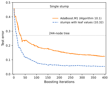
default_rng(10), test set from default_rng(11). Code: ch10_boosting.py, fig_10_2. Reproduces Hastie, Tibshirani and Friedman (2009), Figure 10.2. Download: PDF · SVGNote on the book: what produced Figures 10.2 and 10.3?
The book says AdaBoost.M1 with stumps reaches 5.8% test error after 400 rounds and zero training error after about 250. Our implementation of Algorithm 10.1 picks, at every round, the stump with the smallest weighted error among all thresholds of all inputs (confirmed by brute force), and it agrees with the standard library implementation of two-class AdaBoost (identical \(\alpha_m\) and predictions with the same base learner). It gives 12.45% after 400 rounds, a training error of 6.3% at round 400, and first reaches zero training error only at round 4001. A Gini-split stump base learner gives 11.1%. The book's own Figure 10.9 shows an "AdaBoost" curve that is also at about 12% after 400 rounds.
The book's numbers are what real-valued stumps give: choose the split by the weighted exponential loss and give each side the value \(\tfrac12\log(W_+/W_-)\) of (10.32) (with the factor \(\tfrac12\)). On the same data this reaches 5.8% after 250 rounds, 5.3% after 400, and zero training error for good from about round 240 (first at round 226). We therefore show both curves in Figures 10.2–10.3. The second preset of the AdaBoost demo runs the real-valued version.
10.1.1 Outline of This Chapter
pp. 340–341 The plan: AdaBoost fits an additive model by minimising an exponential loss, close to the binomial log-likelihood (Sections 10.2–10.4); its population minimiser is the log-odds (10.5); more robust losses exist (10.6); trees are the natural base learner for data mining (10.7, 10.9); gradient boosting handles any loss (10.10); slow learning by shrinkage and randomisation helps (10.12); and boosted models can be interpreted (10.13).
10.2 Boosting Fits an Additive Model
pp. 341–342 The combined classifier (10.1) is an expansion in the "basis functions" \(G_m(x)\in\{-1,1\}\). More generally a basis-function expansion has the form
\[ f(x)=\sum_{m=1}^M\beta_m\,b(x;\gamma_m), \tag{10.3} \]with coefficients \(\beta_m\) and simple functions \(b(x;\gamma)\) of the input, each described by a parameter vector \(\gamma\): a sigmoid of a linear combination for single-hidden-layer networks, a shifted and scaled mother wavelet (Section 5.9), a product of hinge functions for MARS, or, for a tree, its split variables, split points and leaf values. Such models are usually fitted by minimising a loss averaged over the data,
\[ \min_{\{\beta_m,\gamma_m\}_1^M}\ \sum_{i=1}^NL\Big(y_i,\sum_{m=1}^M\beta_mb(x_i;\gamma_m)\Big), \tag{10.4} \]which for most losses and basis functions is a hard joint optimisation over all \(M\) terms. Often, though, the problem with a single term is easy:
\[ \min_{\beta,\gamma}\ \sum_{i=1}^NL\big(y_i,\beta\,b(x_i;\gamma)\big). \tag{10.5} \]See also (this course): Section 5.1 for fixed basis expansions; here the basis functions themselves are learned.
10.3 Forward Stagewise Additive Modeling
pp. 342–343 Forward stagewise modelling approximates (10.4) by solving a sequence of problems of the form (10.5): each new term is fitted given the current model, and earlier terms are never revisited.
Algorithm 10.2 (forward stagewise additive modeling) p. 342
- Set \(f_0(x)=0\).
- For \(m=1,\dots,M\):
- compute \[(\beta_m,\gamma_m)=\argmin_{\beta,\gamma}\sum_{i=1}^NL\big(y_i,f_{m-1}(x_i)+\beta\,b(x_i;\gamma)\big);\]
- \(f_m(x)=f_{m-1}(x)+\beta_mb(x;\gamma_m)\).
"Stagewise" is the opposite of "stepwise": a stepwise method re-fits all coefficients when a term enters (Section 3.3.2), a stagewise one freezes them (Section 3.3.3).
Result 10.1 (with squared error, each stage fits the current residuals) p. 343, (10.6)–(10.7)
For the squared-error loss
\[ L(y,f(x))=(y-f(x))^2, \tag{10.6} \]the criterion of step 2(a) is
\[ \sum_{i=1}^N\big(y_i-f_{m-1}(x_i)-\beta\,b(x_i;\gamma)\big)^2=\sum_{i=1}^N\big(r_{im}-\beta\,b(x_i;\gamma)\big)^2, \tag{10.7} \]with \(r_{im}=y_i-f_{m-1}(x_i)\) the current residuals. For fixed \(\gamma\) the best coefficient is the least-squares slope \(\beta(\gamma)=\sum_ir_{im}b(x_i;\gamma)/\sum_ib(x_i;\gamma)^2\), and \(\gamma_m\) maximises \(\big(\sum_ir_{im}b(x_i;\gamma)\big)^2/\sum_ib(x_i;\gamma)^2\), the squared correlation (uncentred) between the residuals and the basis function.
Proof
The first identity is the definition of \(r_{im}\). For fixed \(\gamma\) write \(\bb=(b(x_i;\gamma))_i\) and \(\mathbf r=(r_{im})_i\); the criterion \(\|\mathbf r-\beta\bb\|^2\) is a quadratic in \(\beta\) with minimiser \(\beta=\langle\mathbf r,\bb\rangle/\|\bb\|^2\) (if \(\bb\ne0\)) and minimum value \(\|\mathbf r\|^2-\langle\mathbf r,\bb\rangle^2/\|\bb\|^2\). Minimising this over \(\gamma\) is maximising \(\langle\mathbf r,\bb\rangle^2/\|\bb\|^2\). ∎
This is "least-squares boosting" (Section 10.10.2). Squared error is a poor criterion for classification, though (Section 10.6), which is why other losses are needed.
See also (companion course): Filling the gap 14.10, boosting with squared error fits the residuals.
10.4 Exponential Loss and AdaBoost
pp. 343–344 Now take the base learners to be classifiers \(G(x)\in\{-1,1\}\) and the loss to be the exponential loss
\[ L(y,f(x))=\exp(-y\,f(x)). \tag{10.8} \]Step 2(a) of Algorithm 10.2 asks for
\[ (\beta_m,G_m)=\argmin_{\beta,G}\sum_{i=1}^N\exp\big[-y_i\big(f_{m-1}(x_i)+\beta\,G(x_i)\big)\big]. \]Because \(\exp(a+b)=e^ae^b\), this is
\[ (\beta_m,G_m)=\argmin_{\beta,G}\sum_{i=1}^Nw_i^{(m)}\exp(-\beta\,y_iG(x_i)),\qquad w_i^{(m)}=\exp(-y_if_{m-1}(x_i)), \tag{10.9} \]where the weights do not depend on \(\beta\) or \(G\) but change from round to round through \(f_{m-1}\).
Result 10.2 (AdaBoost.M1 is forward stagewise additive modelling with the exponential loss; Exercise 10.1) pp. 343–344, (10.9)–(10.15)
Let the class of base classifiers be closed under reversal (\(G\) available implies \(-G\) available), and write \(W=\sum_iw_i^{(m)}\). Then:
(a) for every \(\beta>0\) the minimising classifier in (10.9) is the one with the smallest weighted error,
\[ G_m=\argmin_G\sum_{i=1}^Nw_i^{(m)}I(y_i\ne G(x_i)); \tag{10.10} \](b) with \(\err_m\) its weighted error rate,
\[ \err_m=\frac{\sum_{i=1}^Nw_i^{(m)}I(y_i\ne G_m(x_i))}{\sum_{i=1}^Nw_i^{(m)}}, \tag{10.13} \]the minimising coefficient is
\[ \beta_m=\frac12\log\frac{1-\err_m}{\err_m}; \tag{10.12} \](c) the update \(f_m=f_{m-1}+\beta_mG_m\) changes the weights to
\[ w_i^{(m+1)}=w_i^{(m)}\,e^{-\beta_my_iG_m(x_i)} \tag{10.14} \] \[ \phantom{w_i^{(m+1)}}=w_i^{(m)}\,e^{\alpha_mI(y_i\ne G_m(x_i))}\,e^{-\beta_m},\qquad \alpha_m=2\beta_m. \tag{10.15} \]Consequently the weights, classifiers and coefficients of AdaBoost.M1 are those of stagewise exponential-loss fitting, and its output \(\sgn\sum\alpha_mG_m=\sgn(2f_M)\) is the sign of the stagewise fit.
Proof
(a) Since \(y_iG(x_i)=1\) on correctly classified points and \(-1\) on the others,
\[ \sum_iw_i^{(m)}e^{-\beta y_iG(x_i)}=e^{-\beta}\sum_{y_i=G(x_i)}w_i^{(m)}+e^{\beta}\sum_{y_i\ne G(x_i)}w_i^{(m)}, \]and moving the misclassified weight from the first sum to the second,
\[ \sum_iw_i^{(m)}e^{-\beta y_iG(x_i)}=\big(e^{\beta}-e^{-\beta}\big)\sum_{i=1}^Nw_i^{(m)}I(y_i\ne G(x_i))+e^{-\beta}\sum_{i=1}^Nw_i^{(m)}. \tag{10.11} \]For \(\beta>0\) the factor \(e^\beta-e^{-\beta}\) is positive and the second term does not involve \(G\), so the minimiser over \(G\) is (10.10), whatever the value of \(\beta\). Negative \(\beta\) adds nothing: the pair \((\beta,G)\) gives the same term \(\beta G\) as \((-\beta,-G)\), and \(-G\) is in the class.
(b) Write \(\varepsilon(G)\) for the weighted error rate of \(G\). Since \(\varepsilon(-G)=1-\varepsilon(G)\), the minimal rate satisfies \(\err_m\le\tfrac12\). By (10.11) the criterion at \(G_m\) is \(W\varphi(\beta)\), with
\[ \varphi(\beta)=(1-\err_m)e^{-\beta}+\err_m\,e^{\beta}. \]For \(0\lt\err_m\lt1\), \(\varphi\) is strictly convex (\(\varphi''=\varphi>0\)) and tends to infinity at both ends, so its unique minimiser solves \(\varphi'(\beta)=-(1-\err_m)e^{-\beta}+\err_me^{\beta}=0\), that is \(e^{2\beta}=(1-\err_m)/\err_m\), which is (10.12). Its minimum value is
\[ \varphi(\beta_m)=(1-\err_m)\sqrt{\tfrac{\err_m}{1-\err_m}}+\err_m\sqrt{\tfrac{1-\err_m}{\err_m}}=2\sqrt{\err_m(1-\err_m)}. \](If \(\err_m=0\) the infimum is approached as \(\beta\to\infty\): a perfect classifier has nothing left to learn.) The joint minimisation over \((\beta,G)\) is solved by this pair: for any \(G\) with rate \(\varepsilon\ge\err_m\) and any \(\beta>0\), the criterion \(W[(1-\varepsilon)e^{-\beta}+\varepsilon e^{\beta}]\) is at least \(W\varphi(\beta)\ge W\varphi(\beta_m)\).
(c) By definition \(w_i^{(m+1)}=e^{-y_if_m(x_i)}=e^{-y_if_{m-1}(x_i)}e^{-\beta_my_iG_m(x_i)}\), which is (10.14). With \(-y_iG_m(x_i)=2I(y_i\ne G_m(x_i))-1\) this is (10.15). The factor \(e^{-\beta_m}\) multiplies every weight by the same number.
AdaBoost.M1. Both (10.10) and (10.13) are unchanged when all weights are multiplied by a positive constant. By induction on \(m\), the weights of Algorithm 10.1 are \(c_m\,w_i^{(m)}\) with \(c_m>0\): at \(m=1\), \(w_i^{(1)}=e^0=1\) and Algorithm 10.1 uses \(1/N\); if the claim holds at round \(m\), both algorithms choose the same \(G_m\) and \(\err_m\), line 2(c) gives \(\alpha_m=2\beta_m\), and line 2(d) is (10.15) without the common factor \(e^{-\beta_m}\), so \(c_{m+1}=c_me^{\beta_m}\). Finally \(\sum\alpha_mG_m=2\sum\beta_mG_m=2f_M\). ∎
Line 2(a) of AdaBoost, "fit a classifier with weights", is thus an approximate solution of (10.10): a tree grown by a weighted impurity criterion, for instance, approximates the weighted-error minimiser. Our stumps solve (10.10) exactly over all single splits.
See also (companion course): Result 14.4 and Filling the gaps 14.5–14.7, the same derivation in Bishop's notation (with \(\tfrac12\alpha_m\) in place of \(\beta_m\)).
Filling the gap 10.1: the weights are the current losses, and why the training error can reach zero while the loss keeps falling p. 344
By (10.9), \(w_i^{(m)}=e^{-y_if_{m-1}(x_i)}\) is exactly the exponential loss of point \(i\) under the current model: AdaBoost weights each point by how badly it is currently fitted, measured on the margin scale. A point with margin \(-z\lt0\) gets weight \(e^z\), unbounded as \(z\) grows.
Derivation
The identity is the definition of the weights in (10.9) together with Result 10.2(c). Normalised, \(w_i^{(m)}/\sum_kw_k^{(m)}\) is the share of the total training loss carried by point \(i\). Our implementation renormalises the weights after every round, and the weights it ends with agree with \(e^{-y_if_M(x_i)}\) normalised to relative accuracy \(10^{-15}\).
The next result shows that the average loss falls by the factor \(2\sqrt{\err_m(1-\err_m)}\lt1\) at every round. The training error, a step function of the margins, stops changing once all margins are positive, but the loss still falls because the margins keep growing: boosting goes on increasing the confidence of correct classifications. This is why the test error can keep improving after the training error has reached zero (the dashed curves of Figures 10.2–10.3). ∎
Result 10.3 (the training error bound, and the newest classifier is reset to guessing; Freund and Schapire, 1997) pp. 344–345, Figure 10.3
With \(f_M=\sum_m\beta_mG_m\) as in Result 10.2 and \(\gamma_m=\tfrac12-\err_m\),
\[ \frac1N\sum_{i=1}^NI(y_if_M(x_i)\le0)\ \le\ \frac1N\sum_{i=1}^Ne^{-y_if_M(x_i)}=\prod_{m=1}^M2\sqrt{\err_m(1-\err_m)}\ \le\ \exp\Big(-2\sum_{m=1}^M\gamma_m^2\Big). \]Moreover, under the updated weights \(w^{(m+1)}\) the classifier \(G_m\) has weighted error exactly \(\tfrac12\).
Proof
The first inequality holds term by term, since \(I(z\le0)\le e^{-z}\) for every real \(z\). For the equality, \[\sum_ie^{-y_if_m(x_i)}=\sum_iw_i^{(m+1)}=\sum_iw_i^{(m)}e^{-\beta_my_iG_m(x_i)},\] which by the proof of Result 10.2(b) equals \(W_m\varphi(\beta_m)=W_m\cdot2\sqrt{\err_m(1-\err_m)}\), with \(W_m=\sum_iw_i^{(m)}\) and \(W_1=N\). Multiplying over \(m\) and dividing by \(N\) gives the product. For the last inequality, \(2\sqrt{\err(1-\err)}=\sqrt{1-4\gamma^2}\le e^{-2\gamma^2}\) because \(1-u\le e^{-u}\) with \(u=4\gamma^2\).
For the second claim, the misclassified weight after the update is \(\err_me^{\beta_m}W_m\) and the correctly classified weight is \((1-\err_m)e^{-\beta_m}W_m\), both multiplied by the common factor. With \(e^{2\beta_m}=(1-\err_m)/\err_m\) the first equals \(\sqrt{\err_m(1-\err_m)}\,W_m\), and so does the second, so the error under the new weights is \(\tfrac12\). ∎
Each round therefore leaves the newest classifier useless on the new weights, and forces the next one to find something different. On the simulation the product formula holds to \(10^{-14}\) at every round, and the bound explains the shape of Figure 10.3: the loss decreases smoothly and stays above the training error.
See also (companion course): Result 14.3 (the newest classifier reduced to guessing) and Result 14.5 (the training error bound).
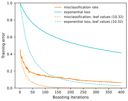
fig_10_3. Reproduces Hastie, Tibshirani and Friedman (2009), Figure 10.3. Download: PDF · SVG10.5 Why Exponential Loss?
pp. 345–346 AdaBoost was designed from a different (computational learning) viewpoint and its link with the exponential loss was noticed only later; the attraction of the loss is computational, the simple reweighting. Statistically, the question is what it estimates, answered by its population minimiser: the function minimising the expected loss at each \(x\).
Result 10.4 (the exponential loss and the deviance both estimate half the log-odds; Exercise 10.2) pp. 345–346, (10.16)–(10.18)
Let \(p(x)=\Pr(Y=1\given x)\in(0,1)\). Then
\[ f^*(x)=\argmin_{f(x)}\E_{Y|x}\big(e^{-Yf(x)}\big)=\frac12\log\frac{\Pr(Y=1\given x)}{\Pr(Y=-1\given x)}, \tag{10.16} \]equivalently \(\Pr(Y=1\given x)=1/(1+e^{-2f^*(x)})\). With the model
\[ p(x)=\Pr(Y=1\given x)=\frac{e^{f(x)}}{e^{-f(x)}+e^{f(x)}}=\frac1{1+e^{-2f(x)}} \tag{10.17} \]and \(Y'=(Y+1)/2\in\{0,1\}\), the binomial log-likelihood
\[ l(Y,p(x))=Y'\log p(x)+(1-Y')\log(1-p(x)) \]gives the deviance
\[ -l(Y,f(x))=\log\big(1+e^{-2Yf(x)}\big), \tag{10.18} \]whose population minimiser is the same \(f^*\). The sign of the AdaBoost expansion is therefore an estimate of the Bayes classifier \(\sgn(p(x)-\tfrac12)\).
Proof
Exponential loss. For fixed \(x\), the expected loss is \(\psi(f)=pe^{-f}+(1-p)e^{f}\), strictly convex with \(\psi(f)\to\infty\) as \(f\to\pm\infty\). Setting \(\psi'(f)=-pe^{-f}+(1-p)e^f=0\) gives \(e^{2f}=p/(1-p)\), which is (10.16); inverting, \(p=e^{2f}/(1+e^{2f})=1/(1+e^{-2f})\). Because \(f(x)\) can be chosen separately at every \(x\), minimising pointwise minimises \(\E_{XY}e^{-Yf(X)}\) over all functions. (If \(p=0\) or \(1\) there is no minimiser: the infimum is approached as \(f\to\mp\infty\).)
Deviance. If \(Y=1\) then \(-\log p=\log(1+e^{-2f})\); if \(Y=-1\) then \(-\log(1-p)=-\log\frac{e^{-2f}}{1+e^{-2f}}=\log(1+e^{2f})\). Both are \(\log(1+e^{-2Yf})\), which is (10.18). Its conditional expectation is \(p\log(1+e^{-2f})+(1-p)\log(1+e^{2f})\), with derivative
\[ -2p\,\frac{e^{-2f}}{1+e^{-2f}}+2(1-p)\frac{e^{2f}}{1+e^{2f}}=-2p(1-\sigma)+2(1-p)\sigma=2(\sigma-p),\qquad\sigma=\frac1{1+e^{-2f}}, \]which vanishes exactly when \(\sigma=p\), i.e. at \(f^*\); the second derivative \(4\sigma(1-\sigma)>0\) makes this the unique minimum. ∎
See also (companion course): Filling the gap 14.8 and Result 14.6 (what each classification error estimates).
Filling the gap 10.2: the exponential loss is not a log-likelihood, and the factor 2 in the logit p. 346
The book remarks that \(e^{-Yf}\) is not the logarithm of any probability mass function. Precisely: if \(-e^{-yf}\) were a log-likelihood, the "probabilities" \(\exp(-e^{-yf})\), \(y=\pm1\), would sum to one; they sum to strictly less than one for every \(f\). Also note the convention: in (10.17) \(f\) is half the logit; gradient boosting with the deviance (Section 10.10, and the spam example (10.24)) uses the full logit \(F=2f\).
Derivation
By symmetry take \(f\ge0\) and put \(a=e^{-f}\in(0,1]\). The sum is \(s(a)=e^{-a}+e^{-1/a}\). At \(a=1\), \(s=2/e\approx0.736\). For \(a\lt1\): first, \(1-e^{-a}=\int_0^ae^{-t}\d t\ge ae^{-a}\). Second, \(e^{-1/a}\lt ae^{-a}\) is equivalent to \(h(a)=\log a-a+1/a>0\); now \(h(1)=0\) and \(h'(a)=-(a^2-a+1)/a^2\lt0\), so \(h\) is decreasing and positive on \((0,1)\). Together, \(e^{-1/a}\lt1-e^{-a}\), i.e. \(s(a)\lt1\). So no normalising constant independent of \(f\) can turn \(e^{-yf}\) into a likelihood: it is a loss, not a model.
For the logit, (10.17) says \(\log\frac{p}{1-p}=2f\). The deviance written with \(F=2f\) and \(y'\in\{0,1\}\) is \(-[y'F-\log(1+e^F)]\), the usual logistic-regression loss of Section 4.4, whose minimiser is the full log-odds. The two parametrisations differ only by the factor 2. ∎
10.6 Loss Functions and Robustness
pp. 346–350 Population minimisers are not the whole story: on a finite sample, losses with the same minimiser weight the observations very differently.
Robust loss functions for classification
The exponential loss and the deviance are both decreasing functions of the margin \(yf(x)\). The margin plays the role of the residual: \(yf>0\) is a correct classification, \(yf\lt0\) an error, and the boundary is \(f(x)=0\). Figure 10.4 shows the candidate losses on the margin scale.
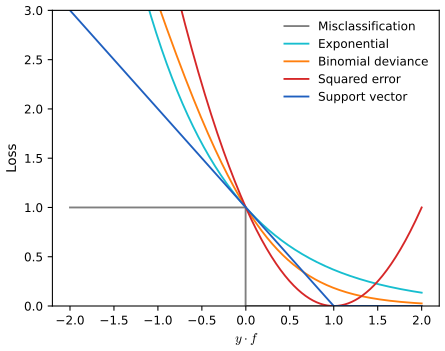
fig_10_4. Reproduces Hastie, Tibshirani and Friedman (2009), Figure 10.4. Download: PDF · SVGResult 10.5 (how much each observation can pull) pp. 347–348, (10.19)
Write a margin-based loss as \(\phi(yf)\). In any gradient-type fit (Section 10.10) the pull of observation \(i\) is \(|\phi'(y_if_i)|\). Then
- exponential, \(\phi(z)=e^{-z}\): \(|\phi'(z)|=e^{-z}\), unbounded as \(z\to-\infty\);
- deviance, \(\phi(z)=\log(1+e^{-2z})\): \(|\phi'(z)|=2/(1+e^{2z})\lt2\), and \(\phi(z)\approx-2z\) for large negative \(z\): the penalty grows only linearly;
- squared error, \(\phi(z)=(1-z)^2\): \(\phi'(z)=-2(1-z)\) changes sign at \(z=1\), so the loss increases with the margin beyond 1, penalising points that are classified correctly with confidence. Its population minimiser is
Proof
The derivatives are direct; for the deviance,
\[ \phi'(z)=-\frac{2e^{-2z}}{1+e^{-2z}}=-\frac2{1+e^{2z}}\in(-2,0), \]and for large negative \(z\), \(\log(1+e^{-2z})=-2z+\log(1+e^{2z})\), which is \(-2z+o(1)\). For (10.19), \(\E(Y-f)^2=\Var(Y\given x)+(\E(Y\given x)-f)^2\) is minimised at \(f=\E(Y\given x)=1\cdot p+(-1)(1-p)=2p-1\). ∎
So the exponential loss concentrates ever more influence on the points with the most negative margins. When the classes overlap or labels are wrong, those points are often unfixable, and AdaBoost spends its effort on them; the deviance spreads the influence more evenly and degrades far less. The label-noise preset of the AdaBoost demo shows the weights piling onto the flipped points. Squared error is not monotone in the margin and is a poor surrogate for misclassification; the "Huberised" squared hinge of Rosset et al. (2004) (Figure 12.4 of the book) keeps the quadratic minimiser (10.19), is zero for \(yf>1\) and linear for \(yf\lt-1\).
With \(K\) classes the Bayes classifier is
\[ G(x)=\mathcal G_k\quad\text{where}\quad k=\argmax_\ell p_\ell(x), \tag{10.20} \]and, as in Section 4.4, the class probabilities are modelled by the multinomial logistic transform
\[ p_k(x)=\frac{e^{f_k(x)}}{\sum_{l=1}^Ke^{f_l(x)}}, \tag{10.21} \]with the symmetric constraint \(\sum_kf_k(x)=0\) instead of setting one function to zero. The deviance becomes the multinomial deviance
\[ L(y,p(x))=-\sum_{k=1}^KI(y=\mathcal G_k)\log p_k(x)=-\sum_{k=1}^KI(y=\mathcal G_k)f_k(x)+\log\Big(\sum_{\ell=1}^Ke^{f_\ell(x)}\Big). \tag{10.22} \]Filling the gap 10.3: the redundancy in (10.21) and the symmetric constraint pp. 348–349; also (10.52)
Adding the same function \(h(x)\) to every \(f_k\) leaves (10.21) unchanged. Among all \((f_1,\dots,f_K)\) that give the same probabilities exactly one sums to zero, namely
\[ f_k(x)=\log p_k(x)-\frac1K\sum_{l=1}^K\log p_l(x), \]which is (10.52) of Section 10.13.2. The two forms of (10.22) agree, and the deviance, like the binomial one, grows only linearly in how wrong the prediction is.
Derivation
Multiplying numerator and denominator of (10.21) by \(e^{h(x)}\) shows the invariance. From (10.21), \(\log p_k=f_k-\log\sum_le^{f_l}\); averaging over \(k\) and using \(\sum_kf_k=0\) gives \(\frac1K\sum_k\log p_k=-\log\sum_le^{f_l}\), and subtracting gives the formula, which also shows uniqueness. For (10.22), \(-\log p_k=-f_k+\log\sum_le^{f_l}\), and only the \(k\) with \(y=\mathcal G_k\) contributes. If the true class is \(k\) and \(f_\ell-f_k=t\) for one wrong class with the others fixed, then \(-\log p_k=\log(1+e^t+\text{const})\approx t\) for large \(t\): linear, not exponential. ∎
A multiclass version of the exponential loss (Zhu et al., 2005) is the subject of Exercise 10.5.
Robust loss functions for regression
For regression, squared error \((y-f)^2\) and absolute error \(|y-f|\) have population minimisers \(\E(Y\given x)\) and \(\med(Y\given x)\), equal for symmetric errors. On samples, squared error lets large residuals dominate, so it degrades badly with long-tailed errors and gross outliers. Huber's (1964) loss for M-regression is a compromise:
\[ L(y,f(x))=\begin{cases}[y-f(x)]^2&\text{for }|y-f(x)|\le\delta,\\2\delta|y-f(x)|-\delta^2&\text{otherwise.}\end{cases} \tag{10.23} \]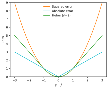
fig_10_5. Reproduces Hastie, Tibshirani and Friedman (2009), Figure 10.5. Download: PDF · SVGFilling the gap 10.4: what Huber's loss does p. 349
\(L_\delta(r)\) of (10.23) is convex and continuously differentiable, with derivative \(\psi_\delta(r)=2r\) for \(|r|\le\delta\) and \(2\delta\,\sgn(r)\) otherwise, bounded by \(2\delta\). The Huber location estimate \(\hat c=\argmin_c\sum_iL_\delta(y_i-c)\) solves \(\sum_i\psi_\delta(y_i-\hat c)=0\): it is a weighted mean of the \(y_i\) with weights \(\min(1,\delta/|y_i-\hat c|)\). As \(\delta\to\infty\) it becomes the mean, and as \(\delta\to0\) a median.
Derivation
At \(|r|=\delta\) both pieces equal \(\delta^2\) and both have slope \(2\delta\sgn(r)\), so \(L_\delta\) is \(C^1\); its derivative is non-decreasing, so it is convex. The estimating equation \(\sum\psi_\delta(y_i-c)=0\) can be written \(\sum_iu_i(y_i-c)=0\) with \(u_i=\psi_\delta(r_i)/(2r_i)=\min(1,\delta/|r_i|)\), so \(c=\sum u_iy_i/\sum u_i\). If \(\delta\) exceeds every \(|y_i-c|\), all \(u_i=1\) and \(c\) is the mean. As \(\delta\to0\), \(\psi_\delta/(2\delta)\to\sgn\) away from zero, and the equation tends to \(\sum\sgn(y_i-c)=0\), which defines a median. A single observation moved to infinity changes the estimating equation by at most \(2\delta\): the influence is bounded. On a skewed sample of 230 points (200 standard normals and 30 shifted exponentials) the Huber estimate with \(\delta=1\) is 0.18, between the median 0.11 and the mean 1.48. ∎
Squared error for regression and exponential loss for classification are not the best criteria statistically, but they are the ones that give simple boosting algorithms (fit the residuals; reweight). Section 10.10 shows how to boost with any differentiable loss.
See also (companion course): Result 14.7 (squared error estimates the mean, absolute error the median) and Figure 14.4.
10.7 “Off-the-Shelf” Procedures for Data Mining
pp. 350–352 No method is best everywhere, and which one will work on a new problem is seldom known in advance. Data-mining problems add their own demands: many observations and variables, inputs of mixed type (quantitative, binary, categorical with many levels), missing values, long-tailed and skewed distributions, gross measurement errors, inputs on very different scales, many irrelevant inputs, and a need for interpretable models. Table 10.1 of the book grades five families (neural networks, support vector machines, trees, MARS, and nearest-neighbour or kernel methods) on these properties. In summary: trees are the only family rated good on mixed data, missing values, outliers in the inputs, invariance to monotone transformations of the inputs, scalability and irrelevant inputs, and fair on interpretability; their weaknesses are predictive accuracy and the inability to form linear combinations of the inputs, where networks and kernel methods are strong.
An off-the-shelf method can be applied to new data without much preprocessing or tuning. Trees come closest: they are fast, handle mixed inputs and missing values (Section 9.2 of the book), are invariant under strictly monotone transformations of each input (a split depends only on the ordering), are immune to outlying inputs, select inputs internally, and resist irrelevant ones. Boosting trees keeps most of these properties and repairs the accuracy, at the price of speed, interpretability and, for AdaBoost, robustness to overlapping classes and mislabelled data. Gradient boosting with robust losses (Section 10.10) addresses the last two.
10.8 Example: Spam Data
pp. 352–353 The spam data (Section 1.2) record, for 4601 e-mails, the frequencies of 48 words and 6 characters and three summaries of runs of capital letters; the book's split has 3065 training and 1536 test e-mails. The book reports a test error of 4.5% for gradient boosting, against 5.5% for an additive logistic regression, 8.7% for a pruned tree and 5.5% for MARS (standard errors about 0.6%; the difference between boosting and the additive model is significant by McNemar's test, Exercise 10.6).
Our model: gradient boosting with the binomial deviance (Algorithm 10.3), 5-leaf trees, shrinkage \(\nu=0.1\), and the number of trees chosen by 5-fold cross-validated deviance on the training set, \(M=431\). Its test error is 4.75% (73 of 1536). With stumps (\(J=2\), an additive model; \(M=1124\) by cross-validation) the test error is 5.14%; the book has 4.7% and 4.5% for the two. On our predictions the two models disagree on 30 test e-mails (18 wrongly classified only by the stump model, 12 only by the 5-leaf model), which McNemar's test does not find significant (\(p=0.27\)). The model is for the log-odds of spam,
\[ f(x)=\log\frac{\Pr(\text{spam}\given x)}{\Pr(\text{email}\given x)}, \tag{10.24} \]the full logit (Filling the gap 10.2). Figures 10.6–10.8 interpret it with the tools of Section 10.13.
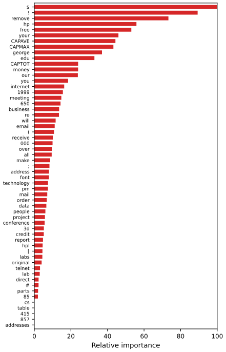
fig_10_6. Reproduces Hastie, Tibshirani and Friedman (2009), Figure 10.6. Download: PDF · SVG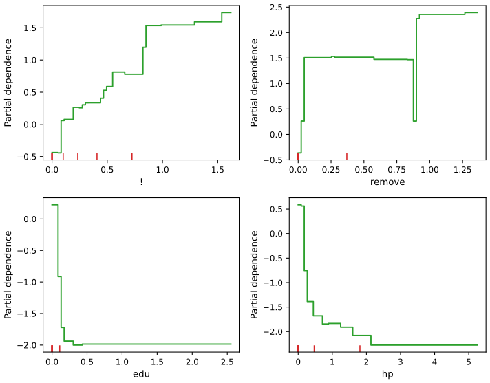
fig_10_7. Reproduces Hastie, Tibshirani and Friedman (2009), Figure 10.7. Download: PDF · SVGThe additive (stump) model is a little worse than the 5-leaf model, which hints at interactions. Two-variable partial dependence plots show them.
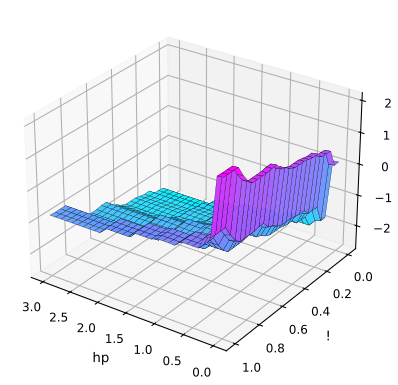
fig_10_8. Reproduces Hastie, Tibshirani and Friedman (2009), Figure 10.8. Download: PDF · SVG10.9 Boosting Trees
pp. 353–358 A tree partitions the input space into regions \(R_1,\dots,R_J\) (its leaves) and predicts a constant in each, \(x\in R_j\Rightarrow f(x)=\gamma_j\):
\[ T(x;\Theta)=\sum_{j=1}^J\gamma_jI(x\in R_j),\qquad\Theta=\{R_j,\gamma_j\}_1^J, \tag{10.25} \]with \(J\) a meta-parameter. Ideally \(\Theta\) minimises the empirical risk
\[ \hat\Theta=\argmin_\Theta\sum_{j=1}^J\sum_{x_i\in R_j}L(y_i,\gamma_j), \tag{10.26} \]a hard combinatorial problem split in two. Given the regions, each \(\gamma_j\) is a one-dimensional location problem (the mean for squared error, the modal class for misclassification loss). The regions are found greedily, top-down, often with a smoother surrogate criterion,
\[ \tilde\Theta=\argmin_\Theta\sum_{i=1}^N\tilde L(y_i,T(x_i,\Theta)), \tag{10.27} \]after which the \(\gamma_j\) are re-estimated with the original loss (for classification trees, the Gini index grows the tree and the leaves predict the majority class). A boosted tree model is a sum of trees,
\[ f_M(x)=\sum_{m=1}^MT(x;\Theta_m), \tag{10.28} \]built by Algorithm 10.2: at step \(m\)
\[ \hat\Theta_m=\argmin_{\Theta_m}\sum_{i=1}^NL\big(y_i,f_{m-1}(x_i)+T(x_i;\Theta_m)\big), \tag{10.29} \]and, given the regions \(R_{jm}\), each leaf value solves a one-dimensional problem,
\[ \hat\gamma_{jm}=\argmin_{\gamma_{jm}}\sum_{x_i\in R_{jm}}L\big(y_i,f_{m-1}(x_i)+\gamma_{jm}\big). \tag{10.30} \]For squared error, (10.29) is just a regression tree fitted to the residuals \(y_i-f_{m-1}(x_i)\) (Result 10.1) with \(\hat\gamma_{jm}\) the mean residual in each leaf. For the exponential loss with "scaled classification trees" \(\beta_mT(x;\Theta_m)\), \(\gamma_{jm}\in\{-1,1\}\), it is AdaBoost (Result 10.2), with the tree minimising the weighted error. Without that restriction (10.29) becomes a weighted exponential criterion for the new tree,
\[ \hat\Theta_m=\argmin_{\Theta_m}\sum_{i=1}^Nw_i^{(m)}\exp[-y_iT(x_i;\Theta_m)], \tag{10.31} \]and the leaf values follow from the next result.
Result 10.6 (leaf values and the splitting criterion for the exponential loss; Exercise 10.7) p. 357, (10.32)
Let \(W_{+}=\sum_{x_i\in R_{jm},\,y_i=1}w_i^{(m)}\) and \(W_{-}=\sum_{x_i\in R_{jm},\,y_i=-1}w_i^{(m)}\) be the weighted class totals of a leaf, both positive. The solution of (10.30) for the exponential loss is
\[ \hat\gamma_{jm}=\frac12\log\frac{\sum_{x_i\in R_{jm}}w_i^{(m)}I(y_i=1)}{\sum_{x_i\in R_{jm}}w_i^{(m)}I(y_i=-1)}=\frac12\log\frac{W_+}{W_-}, \]half the weighted log-odds of the leaf, and the minimised criterion in the leaf is \(2\sqrt{W_+W_-}\). Hence a greedy split of a region into a left and a right part minimises \(\sqrt{W_+^{L}W_-^{L}}+\sqrt{W_+^{R}W_-^{R}}\).
Proof
In the leaf, \(\sum_iw_i^{(m)}e^{-y_i\gamma}=W_+e^{-\gamma}+W_-e^{\gamma}\), strictly convex in \(\gamma\) with derivative \(-W_+e^{-\gamma}+W_-e^{\gamma}\), zero when \(e^{2\gamma}=W_+/W_-\). At that point both terms equal \(\sqrt{W_+W_-}\), so the minimum is \(2\sqrt{W_+W_-}\). The total criterion (10.31) of a tree with optimal leaf values is the sum of these minima over its leaves. If one class is absent from the leaf, the infimum is approached as \(\gamma\to\pm\infty\); in practice a small constant is added to \(W_\pm\). ∎
Note on the book: the factor \(\tfrac12\) in (10.32)
The book prints (10.32) as \(\hat\gamma_{jm}=\log(W_+/W_-)\), without the factor \(\tfrac12\). The minimiser of \(W_+e^{-\gamma}+W_-e^{\gamma}\) is \(\tfrac12\log(W_+/W_-)\) (Result 10.6; Exercise 10.7 asks for exactly this derivation). The missing \(\tfrac12\) is the same one that relates \(\alpha_m\) to \(\beta_m\) in (10.15) and the logit to \(f\) in (10.17). Numerically, on random weights the book's value doubles the optimal step and gives a strictly larger loss, and the version with \(\tfrac12\) is the one that reproduces the numbers quoted for Figures 10.2–10.3.
The book prefers a cheaper approximation to this special tree-growing algorithm: grow the tree by weighted least squares, as described next. With robust losses (absolute error, Huber, the deviance) the leaf problem (10.30) is still easy (a median, or a few Newton steps, usually one), but there is no fast way to solve (10.29) for the regions; approximations like (10.27) are essential.
10.10 Numerical Optimization via Gradient Boosting
pp. 358–361 The training loss of a function \(f\) is
\[ L(f)=\sum_{i=1}^NL(y_i,f(x_i)), \tag{10.33} \]to be minimised over sums of trees (10.28). Ignoring that constraint, it is an ordinary optimisation over the vector of fitted values,
\[ \hat\bff=\argmin_{\bff}L(\bff),\qquad\bff=\{f(x_1),f(x_2),\dots,f(x_N)\}\in\R^N, \tag{10.34} \]and numerical methods build the solution as a sum of steps \(\bff_M=\sum_{m=0}^M\bh_m\), \(\bh_m\in\R^N\), starting from an initial guess \(\bff_0=\bh_0\).
10.10.1 Steepest Descent
Steepest descent takes \(\bh_m=-\rho_m\bg_m\), with \(\bg_m\) the gradient of \(L(\bff)\) at \(\bff_{m-1}\),
\[ g_{im}=\Big[\frac{\partial L(y_i,f(x_i))}{\partial f(x_i)}\Big]_{f(x_i)=f_{m-1}(x_i)}, \tag{10.35} \]and the step length from a line search,
\[ \rho_m=\argmin_\rho L(\bff_{m-1}-\rho\,\bg_m), \tag{10.36} \]then updates \(\bff_m=\bff_{m-1}-\rho_m\bg_m\). The negative gradient is the direction in which \(L\) decreases fastest locally.
10.10.2 Gradient Boosting
Stagewise boosting is greedy too: the tree that solves (10.29) is the most loss-reducing tree, the analogue of the negative gradient, but constrained to be the prediction vector \(\bt_m=(T(x_1;\Theta_m),\dots,T(x_N;\Theta_m))\) of a \(J_m\)-leaf tree; and (10.30) is a line search done separately in each leaf. The gradient is easy for any differentiable loss, while (10.29) is hard for robust losses; but the gradient exists only at the training points, and the goal is a function that generalises. The resolution is to fit a tree to the negative gradient by least squares,
\[ \tilde\Theta_m=\argmin_\Theta\sum_{i=1}^N\big(-g_{im}-T(x_i;\Theta)\big)^2, \tag{10.37} \]a problem for which fast algorithms exist, and then to set the leaf values by (10.30).
Filling the gap 10.5: why a least-squares fit to the negative gradient is a good step pp. 359–360
Fix the regions found by (10.37) and let \(\bt\) be the fitted tree, the vector of leaf means of \(-\bg\). Then \(\bt\) is the orthogonal projection of \(-\bg\) onto the space of vectors constant on each leaf, \(\langle\bt,-\bg\rangle=\|\bt\|^2\ge0\), and the directional derivative of \(L\) along \(\bt\) is \(-\|\bt\|^2\): unless \(\bt=0\), moving a little along the tree lowers the training loss. The leaf-by-leaf line search (10.30) then does at least as well as a single line search along \(\bt\).
Derivation
Let \(\bP\) be the orthogonal projection onto the subspace
\[ V=\{\bh\in\R^N:\ h_i=h_k\text{ whenever }x_i,x_k\text{ share a leaf}\}. \]Minimising \(\|-\bg-\bh\|^2\) over \(\bh\in V\) separates over leaves and gives the leaf means, so \(\bt=\bP(-\bg)\). For a projection, \(\langle\bP\mathbf v,\mathbf v\rangle=\langle\bP\mathbf v,\bP\mathbf v\rangle\), so \(\langle\bt,-\bg\rangle=\|\bt\|^2\). The derivative of \(\rho\mapsto L(\bff+\rho\bt)\) at \(\rho=0\) is \(\langle\nabla L,\bt\rangle=\langle\bg,\bt\rangle=-\|\bt\|^2\lt0\) when \(\bt\ne0\), so \(L(\bff+\rho\bt)\lt L(\bff)\) for all small \(\rho>0\). The vectors \(\rho\bt\) all lie in \(V\), and (10.30) minimises \(L(\bff+\bh)\) over all \(\bh\in V\) (it separates over leaves), so its minimum is no larger than \(\min_\rho L(\bff+\rho\bt)\). For squared error \(-\bg\) is the residual vector and (10.37) is exactly the stagewise problem (10.29). ∎
The negative gradients for the common losses, the pseudo-residuals, are (Table 10.2 of the book):
| setting | loss \(L(y_i,f(x_i))\) | \(-\partial L(y_i,f(x_i))/\partial f(x_i)\) |
|---|---|---|
| regression | \(\tfrac12[y_i-f(x_i)]^2\) | \(y_i-f(x_i)\) |
| regression | \(|y_i-f(x_i)|\) | \(\sgn[y_i-f(x_i)]\) |
| regression | Huber | \(y_i-f(x_i)\) if \(|y_i-f(x_i)|\le\delta_m\); \(\delta_m\sgn[y_i-f(x_i)]\) otherwise, with \(\delta_m\) the \(\alpha\)-quantile of \(\{|y_i-f(x_i)|\}\) |
| classification | deviance (10.22) | \(k\)-th component: \(I(y_i=\mathcal G_k)-p_k(x_i)\) |
Result 10.7 (the pseudo-residuals of Table 10.2 and (10.38)) p. 360
The entries of the table are the negative derivatives of the stated losses, the Huber entry being that of \(\tfrac12L_{\delta_m}\) from (10.23); a constant factor in the pseudo-residuals changes nothing, since the least-squares tree fitted to \(c\,\mathbf r\) has the same regions as the one fitted to \(\mathbf r\). For the deviance (10.22), with \(L\) a function of \(f_1(x_i),\dots,f_K(x_i)\),
\[ -g_{ikm}=-\frac{\partial L\big(y_i,f_{1m}(x_i),\dots,f_{Km}(x_i)\big)}{\partial f_{km}(x_i)}=I(y_i=\mathcal G_k)-p_k(x_i), \tag{10.38} \]so \(K\) least-squares trees are grown at each iteration, one per class, coupled through (10.21).
Proof
\(-\frac{\d}{\d f}\tfrac12(y-f)^2=y-f\); \(-\frac{\d}{\d f}|y-f|=\sgn(y-f)\) for \(y\ne f\); for \(\tfrac12L_\delta(y-f)\), the derivative of Filling the gap 10.4 halved gives \(y-f\) inside and \(\delta\sgn(y-f)\) outside. For (10.22), \(\partial/\partial f_k\) of \(-\sum_ly_lf_l+\log\sum_le^{f_l}\) is \(-y_k+e^{f_k}/\sum_le^{f_l}=-y_k+p_k\). Scale invariance: least squares on \(c\,\mathbf r\) gives every split the improvement \(c^2\) times that on \(\mathbf r\), so the same split wins at every step. (The book's (10.38) has two misprints: the arguments should run \(f_{1m},\dots,f_{Km}\), and the left side is minus the derivative.) A finite-difference check confirms all four entries. ∎
For squared error, (10.37) alone is ordinary least-squares boosting; for absolute error the tree is fitted to the signs of the residuals; Huber's pseudo-residuals are a compromise, clipped at \(\delta_m\). For two classes only one tree per iteration is needed (Exercise 10.10).
10.10.3 Implementations of Gradient Boosting
Algorithm 10.3 (gradient tree boosting) p. 361
- Initialise \(f_0(x)=\argmin_\gamma\sum_{i=1}^NL(y_i,\gamma)\), the best constant.
- For \(m=1,\dots,M\):
- compute the pseudo-residuals \(r_{im}=-\big[\partial L(y_i,f(x_i))/\partial f(x_i)\big]_{f=f_{m-1}}\), \(i=1,\dots,N\);
- fit a regression tree to the targets \(r_{im}\), giving leaves \(R_{jm}\), \(j=1,\dots,J_m\);
- for each leaf, \[\gamma_{jm}=\argmin_\gamma\sum_{x_i\in R_{jm}}L(y_i,f_{m-1}(x_i)+\gamma);\]
- update \[f_m(x)=f_{m-1}(x)+\sum_{j=1}^{J_m}\gamma_{jm}I(x\in R_{jm}).\]
- Output \(\hf(x)=f_M(x)\).
For \(K\) classes, lines 2(a)–(d) are repeated for each class at every iteration, using (10.38); the result is \(K\) coupled expansions \(f_{kM}(x)\) giving probabilities by (10.21) and classes by (10.20) (Algorithm 10.4). The original implementation was called MART; the R package gbm (Ridgeway) and mboost (Hothorn and Bühlmann, 2006) implement it. The tuning parameters are \(M\) and the tree sizes \(J_m\).
Result 10.8 (the leaf values (10.30) for the common losses) pp. 357–361
With \(r_i=y_i-f_{m-1}(x_i)\) for the points of a leaf \(R\) with \(n\) points:
- squared error: \(\gamma=\frac1n\sum_{x_i\in R}r_i\), the mean residual; the initial constant is \(\bar y\);
- absolute error: \(\gamma=\med_{x_i\in R}(r_i)\); the initial constant is \(\med(y_i)\);
- Huber (Friedman, 2001): with \(\tilde r=\med_{x_i\in R}(r_i)\), the one-step estimate \[\gamma=\tilde r+\frac1n\sum_{x_i\in R}\sgn(r_i-\tilde r)\min(\delta_m,|r_i-\tilde r|);\]
- binomial deviance, \(y_i\in\{0,1\}\), \(F\) the log-odds, \(p_i=1/(1+e^{-F(x_i)})\): one Newton step from \(\gamma=0\), \(\gamma=\sum_{x_i\in R}(y_i-p_i)\big/\sum_{x_i\in R}p_i(1-p_i)\); the initial constant is \(\log(\bar y/(1-\bar y))\).
Proof
The first two are the minimisers of \(\sum(r_i-\gamma)^2\) and of \(\sum|r_i-\gamma|\) (any median minimises the latter: the right derivative \(\#\{r_i\le\gamma\}-\#\{r_i>\gamma\}\) changes sign there). For Huber, the minimiser solves \(\sum\psi(r_i-\gamma)=0\) with \(\psi(u)=\sgn(u)\min(\delta,|u|)\) (Filling the gap 10.4, halved). Start at the robust value \(\gamma_0=\tilde r\) and take one step of the fixed-point iteration \(\gamma\leftarrow\gamma+\frac1n\sum\psi(r_i-\gamma)\), whose step size \(1/n\) is the reciprocal of \(\sum\psi'\) when no residual is clipped; the result is the stated formula, and it is exact (the mean) when all \(|r_i-\tilde r|\le\delta\). For the deviance, \(\ell(\gamma)=\sum_{R}[\log(1+e^{F_i+\gamma})-y_i(F_i+\gamma)]\) has \(\ell'(0)=-\sum(y_i-p_i)\) and \(\ell''(0)=\sum p_i(1-p_i)\), and the Newton step is \(-\ell'(0)/\ell''(0)\). The initial constants minimise the loss over constants in the same way; for the deviance, \(\sum(y_i-p)=0\) gives \(p=\bar y\). ∎
Our implementation follows these formulas (\(\alpha=0.9\) for Huber, as in the book's examples), grows each tree best-first to \(J\) leaves on the least-squares criterion, and gives exactly the same fits as a standard library implementation for squared error, the binomial deviance and the \(K\)-class deviance.
Algorithm 10.4 (gradient boosting for \(K\)-class classification) p. 387
- Initialise \(f_{k0}(x)=0\), \(k=1,\dots,K\).
- For \(m=1,\dots,M\):
- set \(p_k(x)=e^{f_k(x)}\big/\sum_{\ell=1}^Ke^{f_\ell(x)}\), \(k=1,\dots,K\);
- for \(k=1,\dots,K\):
- compute \(r_{ikm}=y_{ik}-p_k(x_i)\), \(i=1,\dots,N\);
- fit a regression tree to the targets \(r_{ikm}\), giving leaves \(R_{jkm}\), \(j=1,\dots,J_m\);
- compute, for \(j=1,\dots,J_m\), \[\gamma_{jkm}=\frac{K-1}K\,\frac{\sum_{x_i\in R_{jkm}}r_{ikm}}{\sum_{x_i\in R_{jkm}}|r_{ikm}|(1-|r_{ikm}|)};\]
- update \[f_{km}(x)=f_{k,m-1}(x)+\sum_{j=1}^{J_m}\gamma_{jkm}I(x\in R_{jkm}).\]
- Output \(\hf_k(x)=f_{kM}(x)\), \(k=1,\dots,K\).
Since \(r=y-p\) with \(y\in\{0,1\}\), \(|r|(1-|r|)=p(1-p)\): step iii is a diagonal Newton step scaled by \((K-1)/K\). Its derivation is Exercise 10.8 and Exercise 10.9.
10.11 Right-Sized Trees for Boosting
pp. 361–364 Growing each tree large and pruning it as if it were the last term of the expansion (as for a single tree) produces trees that are far too big, especially early on. The simplest alternative is to give every tree the same number of leaves, \(J_m=J\), a meta-parameter of the whole procedure. The right value depends on the target function, the minimiser of the expected loss,
\[ \eta=\argmin_f\E_{XY}L(Y,f(X)), \tag{10.39} \]and in particular on how its inputs interact, as described by an ANOVA expansion
\[ \eta(X)=\sum_j\eta_j(X_j)+\sum_{jk}\eta_{jk}(X_j,X_k)+\sum_{jkl}\eta_{jkl}(X_j,X_k,X_l)+\cdots. \tag{10.40} \]The first sum holds the main effects, the functions of one input that jointly best approximate \(\eta\); the second the second-order interactions that best improve on them; and so on. In practice low-order interactions tend to dominate, and models that build strong high-order interactions (large trees) lose accuracy.
Result 10.9 (a tree with \(J\) leaves has interaction order at most \(J-1\); boosted stumps are additive) pp. 362–363
A tree with \(J\) leaves is a sum of \(J\) terms, each a function of at most \(J-1\) inputs; hence no interaction of order higher than \(J-1\) can appear in it, nor in any sum of such trees (10.28). In particular, a sum of stumps (\(J=2\)) is additive,
\[ f_M(x)=\sum_{m=1}^MT(x;\Theta_m)=\sum_{j=1}^pf_j(x_j),\qquad f_j(x_j)=\sum_{m:\ \text{tree }m\text{ splits on }j}T(x;\Theta_m), \]a main-effects model, and \(J=3\) allows two-variable interactions.
Proof
A binary tree with \(J\) leaves has \(J-1\) internal nodes. The leaf \(R_j\) is the set where every split on the path from the root to it is satisfied, so \(I(x\in R_j)=\prod_{t\in\text{path}}I(\text{condition }t)\), a function of the inputs split on along that path, of which there are at most \(J-1\). Therefore \(T(x)=\sum_j\gamma_jI(x\in R_j)\) is a sum of functions of at most \(J-1\) inputs each, and so is any sum of such trees. A stump has one split, on input \(j\) say, and is a function of \(x_j\) alone; grouping the stumps by their split input gives the displayed decomposition. In the 5-leaf spam model every leaf depends on at most 4 inputs (as it must), and the two-variable partial dependence of the stump model is exactly additive (Result 10.11). ∎
So \(J\) should reflect the dominant order of interaction of \(\eta\), usually unknown but low. Experience suggests \(4\le J\le8\), with results rather insensitive within that range and \(J\approx6\) a good default; \(J=2\) is often too small and \(J>10\) rarely needed. The simulation (10.2) is additive (a sum of quadratics inside the threshold), so stumps win there (Figure 10.9), and their coordinate functions recover the quadratics (Figure 10.10).
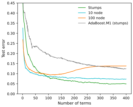
fig_10_9. Reproduces Hastie, Tibshirani and Friedman (2009), Figure 10.9. Download: PDF · SVG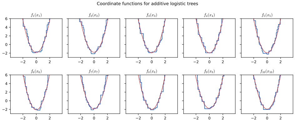
fig_10_10. Reproduces Hastie, Tibshirani and Friedman (2009), Figure 10.10. Download: PDF · SVG10.12 Regularization
pp. 364–367 The other meta-parameter is the number of trees \(M\). Each iteration lowers the training risk, so for large \(M\) the model overfits: there is an optimal \(M^*\), estimated by monitoring a validation sample or by cross-validation, much like early stopping for neural networks (Foundations of Deep Learning, Section 9.3.1).
10.12.1 Shrinkage
Shrinkage scales each tree by a factor \(0\lt\nu\lt1\) when it is added: line 2(d) of Algorithm 10.3 becomes
\[ f_m(x)=f_{m-1}(x)+\nu\cdot\sum_{j=1}^J\gamma_{jm}I(x\in R_{jm}). \tag{10.41} \]\(\nu\) is a learning rate. Smaller \(\nu\) needs larger \(M\) for the same training risk, so the two trade off. Empirically (Friedman, 2001), small \(\nu\) (below 0.1) with \(M\) chosen by early stopping gives much better results than \(\nu=1\), dramatically so for regression and probability estimation and less so for misclassification; the price is computing time, proportional to \(M\).
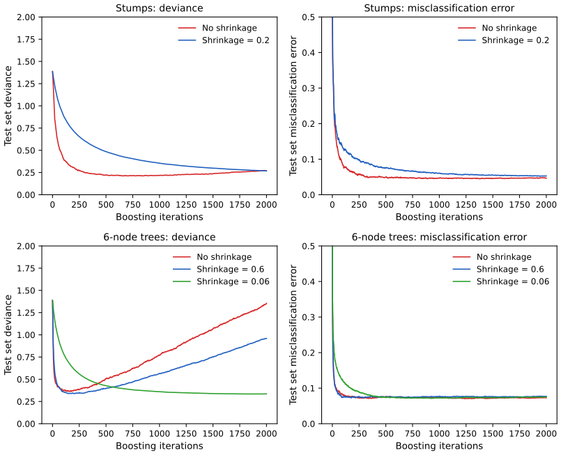
fig_10_11. Reproduces Hastie, Tibshirani and Friedman (2009), Figure 10.11. Download: PDF · SVGFilling the gap 10.6: shrinkage, stagewise fitting and the lasso p. 365, Section 16.2.1
The book only points to Section 16.2.1 for the link between shrinkage and the \(L_1\) penalty. The idea, for orientation: regard every possible tree as a fixed basis function \(T_k\), \(k=1,\dots,K\), so that a boosted model is a linear model \(\sum_k\beta_kT_k(x)\) in a huge dictionary. A shrunken boosting step with squared error changes one coefficient by a small amount in the direction most correlated with the residuals. This is incremental forward stagewise regression with step \(\epsilon\) (Algorithm 3.4, Section 3.8.1); as \(\epsilon\to0\) its coefficient path tends to infinitesimal forward stagewise FS0, which coincides with the lasso path whenever every lasso coefficient profile is monotone (Result 3.26 and the discussion there). So boosting with small \(\nu\) behaves approximately like fitting \(\sum\beta_kT_k\) with a penalty on \(\sum|\beta_k|\), and \(M\) plays the role of the penalty bound.
Why the step is a coordinate move
With squared error and a fixed dictionary, step 2(a)–(b) of Algorithm 10.3 picks the tree (basis function) that best fits the residuals in least squares, i.e. the one maximising \(\langle\br,\bt_k\rangle^2/\|\bt_k\|^2\) (Result 10.1), and (10.41) adds \(\nu\) times its least-squares coefficient: only \(\beta_k\) changes, by \(\nu\langle\br,\bt_k\rangle/\|\bt_k\|^2\). With standardised basis functions and small \(\nu\), this is the move of incremental forward stagewise regression in the direction of the most correlated variable (Algorithm 3.4), with a step proportional to that correlation instead of a fixed \(\epsilon\). The precise statement and its conditions are in Chapter 16 of the book; the point here is only that shrinkage turns greedy stagewise fitting into a slow, regularised path. ∎
10.12.2 Subsampling
Bagging (Section 8.7 of the book) improves a noisy procedure by averaging over bootstrap samples. Stochastic gradient boosting (Friedman, 1999) borrows the idea: at each iteration a fraction \(\eta\) of the training observations is drawn without replacement, and the next tree (regions and leaf values) is grown on that subsample only; everything else is unchanged. A typical value is \(\eta=\tfrac12\), smaller for large \(N\). The computing time drops by the factor \(\eta\), and the model is often more accurate.
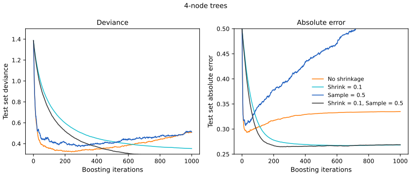
default_rng(12). Code: fig_10_12. Reproduces Hastie, Tibshirani and Friedman (2009), Figure 10.12. Download: PDF · SVGThere are now four tuning parameters, \(J\), \(M\), \(\nu\) and \(\eta\); usually a little exploration fixes \(J\), \(\nu\) and \(\eta\), and \(M\) is chosen by validation.
10.13 Interpretation
pp. 367–370 A single tree can be drawn and read; a sum of hundreds of trees cannot. Two tools replace the picture: measures of how much each input matters, and plots of how the fitted function depends on one or two inputs.
10.13.1 Relative Importance of Predictor Variables
For a single tree \(T\), Breiman et al. (1984) measure the relevance of input \(X_\ell\) by
\[ \mathcal I_\ell^2(T)=\sum_{t=1}^{J-1}\hat\imath_t^2\,I(v(t)=\ell), \tag{10.42} \]the sum over the internal nodes \(t\) that split on \(X_\ell\) (\(v(t)\) is the splitting input) of the improvement \(\hat\imath_t^2\) in squared-error risk brought by the split. For a sum of trees the measure is averaged,
\[ \mathcal I_\ell^2=\frac1M\sum_{m=1}^M\mathcal I_\ell^2(T_m), \tag{10.43} \]which is more stable than (10.42) thanks to the averaging, and suffers less from masking by correlated inputs because of shrinkage. These are squared relevances; the relevances are their square roots, and since only relative values matter the largest is set to 100. For \(K\) classes there are \(K\) expansions
\[ f_k(x)=\sum_{m=1}^MT_{km}(x), \tag{10.44} \]and the measure is computed per class and then averaged over classes:
\[ \mathcal I_{\ell k}^2=\frac1M\sum_{m=1}^M\mathcal I_\ell^2(T_{km}), \tag{10.45} \] \[ \mathcal I_\ell^2=\frac1K\sum_{k=1}^K\mathcal I_{\ell k}^2. \tag{10.46} \]Result 10.10 (the improvement of a split, and what the importances add up to) p. 368
A node with \(n\) points and targets \(g_i\) split into parts with \(n_L\) and \(n_R\) points, sums \(G_L,G_R\) and means \(\bar g_L,\bar g_R\) has improvement
\[ \hat\imath^2=\frac{G_L^2}{n_L}+\frac{G_R^2}{n_R}-\frac{(G_L+G_R)^2}{n}=\frac{n_Ln_R}{n}\,(\bar g_L-\bar g_R)^2. \]Summed over all inputs, \(\sum_\ell\mathcal I^2_\ell(T)\) is the total decrease of the residual sum of squares achieved by the tree, relative to fitting a constant.
Proof
The residual sum of squares of a node fitted by its mean is \(\sum g_i^2-G^2/n\); a split replaces \(G^2/n\) by \(G_L^2/n_L+G_R^2/n_R\), so the decrease is the first expression. With \(G_L=n_L\bar g_L\), \(G_R=n_R\bar g_R\) and \(n=n_L+n_R\), it equals
\[ n_L\bar g_L^2+n_R\bar g_R^2-\frac{(n_L\bar g_L+n_R\bar g_R)^2}{n}=\frac{n_Ln_R}{n}(\bar g_L-\bar g_R)^2. \]Growing a tree is a sequence of splits, each lowering the residual sum of squares by its improvement; adding them up over all internal nodes, grouped by splitting input, gives the second claim. In gradient boosting the targets are the pseudo-residuals, so the importance measures how much each input helps fit the gradients. ∎
See also (companion course): Result 14.8, what one split gains.
10.13.2 Partial Dependence Plots
Functions of one or two inputs can be drawn; functions of more cannot, except by conditioning on values of the others (trellis plots). A useful substitute is a collection of plots of the partial dependence of \(f(X)\) on small subsets of inputs. Let \(X_S\), \(S\subset\{1,\dots,p\}\), be \(\ell\lt p\) of the inputs and \(X_C\) the rest, so \(f(X)=f(X_S,X_C)\). The partial dependence of \(f\) on \(X_S\) is the marginal average
\[ f_S(X_S)=\E_{X_C}f(X_S,X_C), \tag{10.47} \]estimated from the training data by
\[ \bar f_S(X_S)=\frac1N\sum_{i=1}^Nf(X_S,x_{iC}), \tag{10.48} \]where \(x_{1C},\dots,x_{NC}\) are the values of \(X_C\) in the training set. It applies to any "black box", at the cost of a pass over the data for every value of \(X_S\); for trees that cost can be cut (Result 10.13). It is not the effect of \(X_S\) ignoring the other inputs, which is the conditional expectation
\[ \tilde f_S(X_S)=\E\big(f(X_S,X_C)\given X_S\big), \tag{10.49} \]the best least-squares approximation of \(f(X)\) by a function of \(X_S\) alone. The two agree when \(X_S\) and \(X_C\) are independent, and generally not otherwise. Two special structures show the difference:
\[ f(X)=h_1(X_S)+h_2(X_C), \tag{10.50} \] \[ f(X)=h_1(X_S)\cdot h_2(X_C). \tag{10.51} \]Result 10.11 (partial dependence recovers additive and multiplicative components; Exercise 10.3) pp. 369–370
Under (10.50), \(f_S=h_1+\E h_2(X_C)\): \(h_1\) up to an additive constant. Under (10.51), \(f_S=h_1\cdot\E h_2(X_C)\): \(h_1\) up to a constant factor. Both hold exactly for the sample version (10.48), with the expectations replaced by averages over the training \(x_{iC}\). The conditional expectation gives \(h_1+\E(h_2(X_C)\given X_S)\) and \(h_1\cdot\E(h_2(X_C)\given X_S)\), which recover \(h_1\) only if the conditional expectation of \(h_2(X_C)\) does not depend on \(X_S\). Consequently, for a sum of stumps every two-variable partial dependence \(\bar f_{jk}\) equals \(\bar f_j+\bar f_k\) up to a constant, and the interaction statistic of Friedman and Popescu (2008),
\[ H_{jk}^2=\frac{\sum_i\big[\bar f_{jk}(x_{ij},x_{ik})-\bar f_j(x_{ij})-\bar f_k(x_{ik})\big]^2}{\sum_i\bar f_{jk}(x_{ij},x_{ik})^2}\qquad(\text{each }\bar f\text{ centred}), \]is exactly zero.
Proof
Under (10.50), with the population or the sample average over \(X_C\),
\[ \E_{X_C}[h_1(x_S)+h_2(X_C)]=h_1(x_S)+\E h_2(X_C),\qquad \frac1N\sum_i[h_1(x_S)+h_2(x_{iC})]=h_1(x_S)+\frac1N\sum_ih_2(x_{iC}), \]the second terms constants. Under (10.51) the same computation gives \(h_1(x_S)\) times \(\E h_2(X_C)\) (or its sample average), a constant factor (useful when it is not zero). For (10.49), conditioning on \(X_S\) keeps \(h_1(X_S)\) and replaces \(h_2(X_C)\) by \(\E(h_2(X_C)\given X_S)\), a function of \(X_S\) in general. For stumps, \(f=\sum_jf_j(x_j)\) (Result 10.9); with \(S=\{j,k\}\), (10.50) holds with \(h_1=f_j+f_k\), so \(\bar f_{jk}=f_j+f_k+c\), \(\bar f_j=f_j+c_j\), \(\bar f_k=f_k+c_k\), and after centring the numerator of \(H^2\) vanishes. A simulation with correlated Gaussian inputs confirms both recoveries to rounding error, while the conditional expectation is off by a function of range 1.15; on the spam data \(H\) is \(10^{-15}\) for the stump model and 0.21 for the pair \((!,\text{remove})\) of the 5-leaf model. ∎
Result 10.12 (the conditional expectation can show an effect where there is none; Exercise 10.12) pp. 370, 386
Let \((X_1,X_2)\) be bivariate normal with means 0, variances 1 and correlation \(\rho\), and \(f(X_1,X_2)=X_1\). With \(S=\{2\}\), \(C=\{1\}\): the partial dependence on \(X_2\) is the constant \(\E X_1=0\), correctly showing no dependence, while the conditional expectation is \(\E(f(X_1,X_2)\given X_2)=\rho X_2\), a strong effect of an input that \(f\) does not use.
Proof
\(f_{\{2\}}(x_2)=\E_{X_1}X_1=0\) for all \(x_2\). For the conditional expectation write \(X_1=\rho X_2+\sqrt{1-\rho^2}\,Z\) with \(Z=(X_1-\rho X_2)/\sqrt{1-\rho^2}\). Then \(Z\) is normal with mean 0, \(\Cov(Z,X_2)=(\rho-\rho)/\sqrt{1-\rho^2}=0\), and \(\Var Z=(1-2\rho^2+\rho^2)/(1-\rho^2)=1\); jointly normal and uncorrelated, \(Z\) and \(X_2\) are independent. Hence \(\E(X_1\given X_2)=\rho X_2+\sqrt{1-\rho^2}\,\E Z=\rho X_2\). (The book's statement of the exercise writes \(\E(X_1,X_2)=\rho\) for \(\E(X_1X_2)=\rho\).) ∎
Result 10.13 (partial dependence of a sum of trees, exactly and quickly; Exercise 10.11) p. 370
For a tree, each leaf \(R\) is described by the conditions on its path; split them into the conditions on inputs in \(S\) and those on inputs in \(C\). Let \(\pi_C(R)\) be the fraction of training points whose \(x_C\) satisfies the \(C\)-conditions of \(R\). Then
\[ \bar f_S(x_S)=\sum_{\text{leaves }R}\gamma_R\,\pi_C(R)\,I\big(x_S\text{ satisfies the }S\text{-conditions of }R\big), \]and for a sum of trees one adds these expressions (plus the initial constant). The fractions \(\pi_C(R)\) do not depend on \(x_S\): one pass over the data per tree computes them, after which every evaluation costs one membership test per leaf, instead of a pass over the \(N\) training points per value of \(x_S\).
Proof
For a single tree, \(T(x)=\sum_R\gamma_RI(x\in R)\) and \(I(x\in R)=I(x_S\in A_R)\,I(x_C\in B_R)\), where \(A_R\) and \(B_R\) are the sets defined by the \(S\)- and \(C\)-conditions (each condition involves one input, so the product splits). Hence
\[ \frac1N\sum_{i=1}^NT(x_S,x_{iC})=\sum_R\gamma_RI(x_S\in A_R)\,\frac1N\sum_{i=1}^NI(x_{iC}\in B_R)=\sum_R\gamma_RI(x_S\in A_R)\,\pi_C(R). \]Both (10.48) and the formula are linear in the function, so they add over trees. On the spam model this agrees with the brute-force average (10.48) to \(10^{-14}\), for one and for two inputs. ∎
Note on the book: "without reference to the data"
The book says that for trees (10.48) can be computed from the tree itself, without the data. The usual data-free recipe (Friedman, 2001) sends \(x_S\) down the tree, following the branch at splits on \(S\) and both branches at splits on \(C\), weighted by the training counts \(n_{\text{child}}/n_{\text{node}}\). Its weight for a leaf is a product of conditional fractions given the whole path, \(S\)-splits included, whereas (10.48) needs the unconditional fraction \(\pi_C(R)\). The two agree when no \(C\)-split lies below an \(S\)-split (for stumps, always) or when \(X_S\) and \(X_C\) are independent in the training sample; otherwise the recipe is an approximation. On the spam data it is exact for the stump model and off by up to 0.24 on the logit scale for the partial dependence on \(!\) in the 5-leaf model (the demo's "data-free tree traversal" switch shows it).
Plots of partial dependence on small subsets (\(\ell\approx1,2,3\)) of the most relevant inputs are the most informative, especially for subsets whose effect is close to additive or multiplicative. For \(K\) classes each expansion relates to the probabilities by
\[ f_k(X)=\log p_k(X)-\frac1K\sum_{l=1}^K\log p_l(X), \tag{10.52} \](Filling the gap 10.3), a monotone function of \(p_k\) on the log scale; plotting the partial dependence of each \(f_k\) on its most relevant inputs (10.45) shows how the log-odds of each class depend on them.
10.14 Illustrations
10.14.1 California Housing
pp. 371–375 The data (Pace and Barry, 1997) describe the census block groups of California in 1990: the response is the median house value (in units of $100,000), the eight inputs are median income MedInc, house age HouseAge, average numbers of rooms and bedrooms AveRooms and AveBedrms, population Population, average occupancy AveOccup, and the location (Latitude, Longitude). We use the copy distributed with scikit-learn (20,640 block groups; the book has 20,460), split at random into 80% training and 20% test, and fit gradient boosting with 6-leaf trees, \(\nu=0.1\) and the Huber loss (\(\alpha=0.9\)), as in the book. Figure 10.13 tracks the average absolute error
\[ \AAE=\E\,|y-\hf_M(x)|. \tag{10.53} \]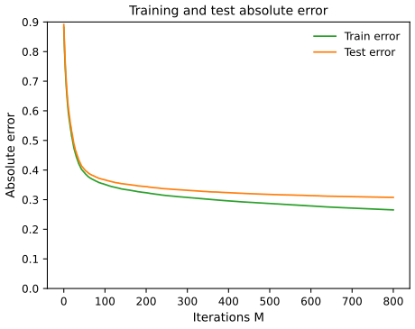
fig_10_13. Reproduces Hastie, Tibshirani and Friedman (2009), Figure 10.13. Download: PDF · SVG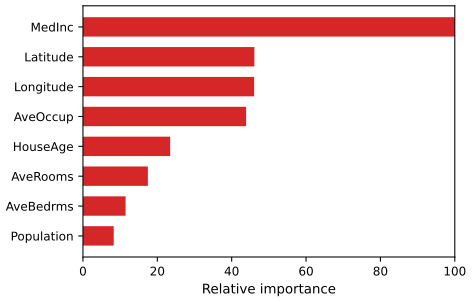
fig_10_14. Reproduces Hastie, Tibshirani and Friedman (2009), Figure 10.14. Download: PDF · SVG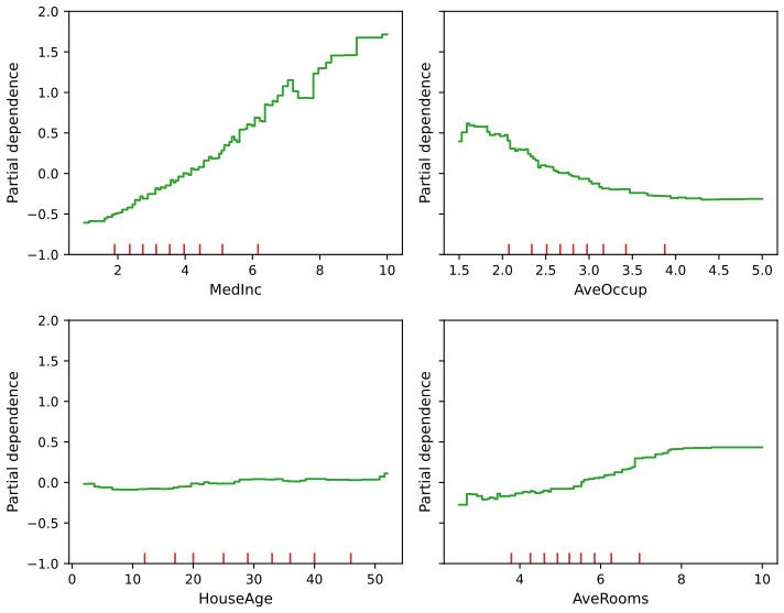
fig_10_15. Reproduces Hastie, Tibshirani and Friedman (2009), Figure 10.15. Download: PDF · SVGThe weak main effect of house age, despite its moderate importance, suggests that it acts through interactions. Figure 10.16 shows one.
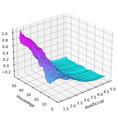
fig_10_16. Reproduces Hastie, Tibshirani and Friedman (2009), Figure 10.16. Download: PDF · SVG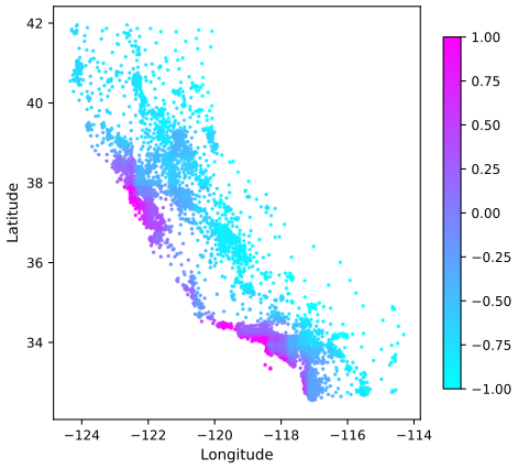
fig_10_17. Reproduces Hastie, Tibshirani and Friedman (2009), Figure 10.17. Download: PDF · SVG10.14.2 New Zealand Fish
pp. 375–379 This example models the presence and the catch of the Black Oreo Dory in about 17,000 research trawls around New Zealand, using depth, temperature and salinity residuals (adjusted for depth), the gradient of the sea-surface temperature, chlorophyll, suspended particulate matter and trawl characteristics (Leathwick et al., 2006). The trawl data are not distributed with the book, so Figures 10.18–10.21 are not reproduced; the same tools appear above. Presence is modelled by gradient-boosted logistic regression (depth-10 trees, \(\nu=0.025\)); its 10-fold cross-validated deviance improves modestly on a generalised additive model with 8 degrees of freedom per term, and the areas under the ROC curves are 0.98 and 0.97. The catch size is modelled with
\[ \E(Y\given X)=\E(Y\given Y>0,X)\cdot\Pr(Y>0\given X). \tag{10.54} \]Filling the gap 10.7: the two-part ("hurdle") decomposition (10.54), and un-logging p. 376
For a non-negative response, (10.54) holds exactly, so presence (a binary model) and positive catch (a model fitted to the trawls with a catch) can be estimated separately. If the positive part is fitted on the log scale, \(\exp\{\E(\log Y\given Y>0,X)\}\) underestimates \(\E(Y\given Y>0,X)\).
Derivation
Since \(Y\ge0\), \(Y=Y\,I(Y>0)\), so
\[ \E(Y\given X)=\E(Y I(Y>0)\given X)=\E(Y\given Y>0,X)\Pr(Y>0\given X) \]by the definition of conditional expectation given an event of positive probability (if \(\Pr(Y>0\given X)=0\) both sides are 0). For the second claim, \(\log\) is concave, so by Jensen's inequality \(\E(\log Y\given\cdot)\le\log\E(Y\given\cdot)\), and exponentiating, \(e^{\E(\log Y\given\cdot)}\le\E(Y\given\cdot)\), with equality only if \(Y\) is constant given the conditioning. If \(\log Y\) given the inputs is normal with variance \(\sigma^2\), the factor is exactly \(e^{\sigma^2/2}\). ∎
The relative influence of the presence model is dominated by temperature residual and depth, and the partial dependence plots show a well-defined depth range and a preference for colder water; because the inputs come from environmental maps, the fitted models can be drawn as prediction maps.
10.14.3 Demographics Data
pp. 379–383 The goal is to predict occupation (nine classes) from 13 other demographic variables collected from shopping-mall customers in the San Francisco Bay Area. We use the book's "marketing" data file (8993 questionnaires; the book's analysis used a 9243-questionnaire version), drop the rows with occupation missing, code a missing input as its own lowest category, split at random 80/20, and fit Algorithm 10.4 with 6-leaf trees and \(\nu=0.1\), as in the book, with the number of rounds chosen by 5-fold cross-validated deviance (59 rounds of nine trees).
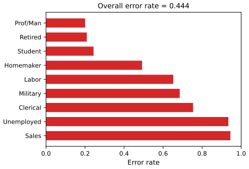
fig_10_22. Reproduces Hastie, Tibshirani and Friedman (2009), Figure 10.22. Download: PDF · SVG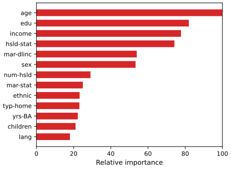
fig_10_23. Reproduces Hastie, Tibshirani and Friedman (2009), Figure 10.23. Download: PDF · SVG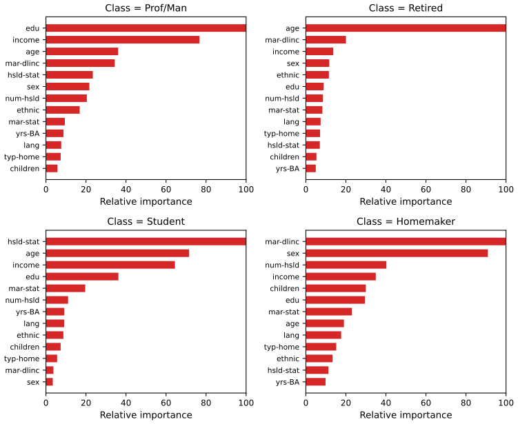
fig_10_24. Reproduces Hastie, Tibshirani and Friedman (2009), Figure 10.24. Download: PDF · SVG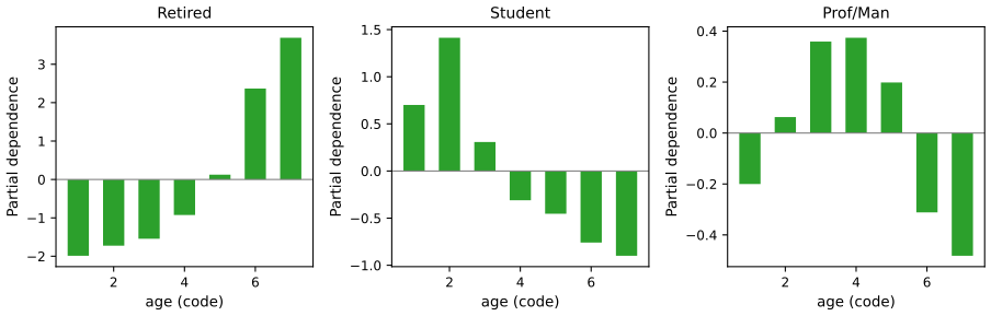
fig_10_25. Reproduces Hastie, Tibshirani and Friedman (2009), Figure 10.25. Download: PDF · SVGBibliographic notes. pp. 380–384 Schapire (1990) gave the first boosting procedure, in the PAC framework: train \(G_2\) on data half of which \(G_1\) misclassifies, \(G_3\) on points where they disagree, and take the majority vote. Freund (1995) proposed boosting by majority, and Freund and Schapire's AdaBoost (1996, 1997) removed the need to know the weak learner's error rate in advance. The theory of the computational learning literature (generalisation bounds, game theory, VC theory) tends to be too loose to explain practice. The statistical view of this chapter comes from Friedman et al. (2000) (exponential loss, additive models, right-sized trees, the multiclass logit) and Friedman (2001) (gradient boosting and shrinkage); Friedman (1999) introduced subsampling, and Mason et al. (2000) took a gradient view as well. Later work studied the consistency of boosting; Bühlmann and Hothorn (2007) survey the area.
Exercises
All 12 exercises of Chapter 10 (Hastie, Tibshirani and Friedman, 2009, pp. 384–386), restated in my own words, with complete solutions (hidden).
Exercise 10.1. Derive the AdaBoost coefficient (10.12).
Solution
This is part (b) of Result 10.2. In brief: by (10.11) the criterion at the weighted-error minimiser \(G_m\) is \(W[(1-\err_m)e^{-\beta}+\err_me^\beta]\); its derivative in \(\beta\) is \(W[-(1-\err_m)e^{-\beta}+\err_me^\beta]\), zero when \(e^{2\beta}=(1-\err_m)/\err_m\), so \(\beta_m=\tfrac12\log\frac{1-\err_m}{\err_m}\); the second derivative \(W[(1-\err_m)e^{-\beta}+\err_me^\beta]>0\) makes it the unique minimum. If \(\err_m>\tfrac12\) the formula gives \(\beta_m\lt0\), the same as reversing \(G_m\). A numerical minimisation of (10.11) confirms the formula for \(\err_m\in\{0.1,0.3,0.45,0.7\}\).
Exercise 10.2. Show that the population minimiser of the AdaBoost criterion, \(\E_{Y|x}e^{-Yf(x)}\), is half the log-odds (10.16).
Solution
Result 10.4: at each \(x\) minimise \(pe^{-f}+(1-p)e^{f}\), strictly convex, with stationary point \(e^{2f}=p/(1-p)\). Pointwise minimisation is legitimate because \(\E_{XY}e^{-Yf(X)}=\E_X\big[\E_{Y|X}e^{-Yf(X)}\big]\) and \(f(x)\) can be chosen separately for each \(x\).
Exercise 10.3. Show that the marginal average (10.47) recovers additive and multiplicative functions (10.50)–(10.51), while the conditional expectation (10.49) does not.
Solution
Result 10.11. For an explicit failure of (10.49), take \(X_S=X_1\), \(X_C=X_2\) jointly normal with correlation \(\rho\neq0\), and \(f=h_1(X_1)+X_2\): then \(f_S=h_1(x_1)+0\) while \(\tilde f_S=h_1(x_1)+\rho x_1\) (Result 10.12), a different function; with \(f=h_1(X_1)X_2\), \(f_S\equiv0\) (because \(\E X_2=0\), the constant factor is 0) while \(\tilde f_S=\rho x_1h_1(x_1)\). Numerically, with \(\rho=0.7\), \(h_1(x)=\sin x+x^2\) and \(h_2(x)=e^{x/2}\), the sample partial dependence equals \(h_1\) plus a constant and \(h_1\) times a constant to rounding error, while the conditional expectation differs from \(h_1\) by a function with range 1.15 over \([-1.5,1.5]\).
Exercise 10.4. (a) Program AdaBoost with trees. (b) Redo Figure 10.2, plotting the training error as well, and discuss it. (c) How many iterations does it take for the test error to start rising? (d) Repeat with overlapping classes: class 1 is ten independent standard normals; class 2 is the same, conditioned on \(\sum_jX_j^2>12\).
Solution
(a)
adaboost_m1in the chapter code implements Algorithm 10.1 with exact weighted-error stumps (every threshold of every input, from sorted cumulative weight sums) or with any weighted classifier, e.g. a classification tree; with the same base learner it reproduces the standard library's two-class AdaBoost exactly.(b) Figures 10.2 and 10.3. The training error falls together with the test error at first and stays a little below it; the exponential loss falls more smoothly and stays above the training error, as the bound of Result 10.3 requires. With AdaBoost.M1 the training error is still 6.3% at round 400, and the test error 12.45%; stumps with real-valued leaves (10.32) reach the book's 5.8% (see the note).
(c) Very many. We ran 10,000 rounds (Figure 10.S1, left). The training error first reaches zero at round 4001. The test error keeps falling until round 3245 (7.96%) and then rises only slowly, to 8.66% at round 10,000: AdaBoost overfits on these noise-free data, but very slowly, because the exponential loss keeps increasing the margins of already correct points rather than chasing a few hard ones.
(d) The Bayes rule classifies as class 2 exactly when \(\sum x_j^2>12\), and its error is \(\tfrac12\Pr(\chi^2_{10}>12)=0.1425\) (a class-1 point lies beyond the threshold with probability 0.285, class 1 is half of the population, and class-2 points are never misclassified). AdaBoost.M1 with stumps (2000 training points, half of each class) reaches its lowest test error, 26.8%, at round 409, then gets worse, 29.0% at round 5000, while its training error keeps falling (8.0%): the class-1 points beyond the threshold are unavoidable errors, and the exponential loss gives them ever larger weights (Result 10.5). Gradient boosting with the binomial deviance, stumps and \(\nu=0.1\) does better (23.1% at its best, 24.4% at round 5000). Both remain far from the Bayes error with 2000 points: the posterior is a step in \(\sum x_j^2\), poorly approximated by a sum of stumps with this much class overlap. The fourth preset of the AdaBoost demo shows the weights moving onto those points.
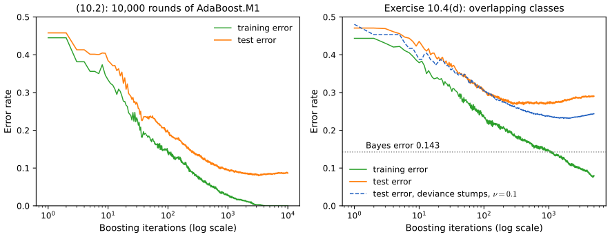
Figure 10.S1 (supplementary, Exercise 10.4). Left: AdaBoost.M1 with stumps on the simulation (10.2) for 10,000 rounds. Right: overlapping classes of Exercise 10.4(d) (training default_rng(16), testdefault_rng(17), 10,000 test points): AdaBoost.M1 and, dashed, gradient boosting with the binomial deviance, stumps and \(\nu=0.1\); the dotted line is the Bayes error. Code:fig_10_s1. Download: PDF · SVGExercise 10.5 (multiclass exponential loss; Zhu et al., 2005). Code the class as \(Y=(Y_1,\dots,Y_K)^\T\) with \(Y_k=1\) if \(G=\mathcal G_k\) and \(-1/(K-1)\) otherwise,
\[ Y_k=\begin{cases}1,&\text{if }G=\mathcal G_k,\\-\frac1{K-1},&\text{otherwise,}\end{cases} \tag{10.55} \]let \(f=(f_1,\dots,f_K)^\T\) with \(\sum_kf_k=0\), and
\[ L(Y,f)=\exp\Big(-\frac1KY^\T f\Big). \tag{10.56} \](a) Using Lagrange multipliers, find the population minimiser \(f^*\) under the zero-sum constraint and relate it to the class probabilities. (b) Show that stagewise boosting with this loss gives a reweighting algorithm like AdaBoost.
Solution
A simplification. If the class is \(c\), then, using \(\sum_{k\ne c}f_k=-f_c\),
\[ Y^\T f=f_c-\frac1{K-1}\sum_{k\ne c}f_k=f_c+\frac{f_c}{K-1}=\frac K{K-1}f_c, \]so \(L=\exp(-f_c/(K-1))\).
(a) The conditional risk is \(\sum_kp_ke^{-f_k/(K-1)}\), to be minimised subject to \(\sum_kf_k=0\). The Lagrangian \(\sum_kp_ke^{-f_k/(K-1)}-\lambda\sum_kf_k\) has stationarity conditions \(-\frac{p_k}{K-1}e^{-f_k/(K-1)}=\lambda\) for all \(k\), so \(p_ke^{-f_k/(K-1)}\) is the same for all \(k\): \(f_k=(K-1)(\log p_k-c)\). The constraint gives \(c=\frac1K\sum_l\log p_l\), hence
\[ f_k^*=(K-1)\Big(\log p_k-\frac1K\sum_{l=1}^K\log p_l\Big),\qquad p_k=\frac{e^{f_k^*/(K-1)}}{\sum_le^{f_l^*/(K-1)}}. \]The risk is a sum of convex functions and the constraint is linear, so the stationary point is the global minimum (all \(p_k>0\) assumed). For \(K=2\), \(f_1^*=\tfrac12\log(p_1/p_2)\), which is (10.16). A numerical minimisation for \(p=(0.5,0.3,0.2)\) confirms the formula.
(b) Let a classifier \(G\) with values in the classes be coded as the vector \(g(x)\) with \(g_k=1\) if \(G(x)=\mathcal G_k\) and \(-1/(K-1)\) otherwise (so \(\sum_kg_k=0\)), and update \(f_m=f_{m-1}+\beta g\). With \(w_i=\exp(-\frac1KY_i^\T f_{m-1}(x_i))\), the criterion is \(\sum_iw_i\exp(-\frac\beta KY_i^\T g(x_i))\). If \(G(x_i)\) is the true class, \(Y_i^\T g=1+(K-1)\frac1{(K-1)^2}=\frac K{K-1}\); if it is a wrong class, \(Y_i^\T g=-\frac2{K-1}+\frac{K-2}{(K-1)^2}=-\frac K{(K-1)^2}\). Hence the criterion is
\[ W\Big[(1-\err)\,e^{-\beta/(K-1)}+\err\,e^{\beta/(K-1)^2}\Big],\qquad\err=\frac{\sum_iw_iI(y_i\ne G(x_i))}{\sum_iw_i}. \]For \(\beta>0\) it is minimised by the classifier with the smallest weighted error, and then by
\[ \beta=\frac{(K-1)^2}K\Big(\log\frac{1-\err}{\err}+\log(K-1)\Big). \]After the step, misclassified points have their weights multiplied by \(e^{\beta/(K-1)^2}\) and correct ones by \(e^{-\beta/(K-1)}\); the ratio is \(e^{\beta K/(K-1)^2}=e^{\alpha}\) with \(\alpha=\log\frac{1-\err}{\err}+\log(K-1)\). After normalisation this is AdaBoost.M1's update with \(\alpha\) increased by \(\log(K-1)\) (the "SAMME" algorithm); it needs only \(\err\lt(K-1)/K\), better than random guessing among \(K\) classes, rather than \(\err\lt\tfrac12\). The classifier is \(\argmax_k\sum_m\alpha_mI(G_m(x)=\mathcal G_k)\). The formula for \(\beta\) and the weight ratio are confirmed numerically for \(K=3\).
Exercise 10.6 (McNemar's test). On the 1536 spam test e-mails the book reports 5.5% error for an additive model (GAM) and 4.5% for gradient boosting (GBM). (a) Show that their standard errors are about 0.6%. (b) Using the table of joint outcomes (both correct 1434; GAM correct and GBM wrong 18; GAM wrong and GBM correct 33; both wrong 51), show that the GAM makes significantly more errors, with a two-sided \(p\)-value of 0.036.
Solution
(a) A test error is a binomial proportion: \(\sqrt{0.055\cdot0.945/1536}=0.0058\) and \(\sqrt{0.045\cdot0.955/1536}=0.0053\), both about 0.6%. The table agrees: GAM errors \(33+51=84=5.47\%\), GBM errors \(18+51=69=4.49\%\).
(b) Because both methods are scored on the same e-mails, their errors are correlated and a two-sample test is wrong. The e-mails on which they agree carry no information about which is better; under the null hypothesis of equal error rates each of the \(b+c=51\) discordant e-mails is equally likely to go either way, so \(b\sim\mathrm{Bin}(51,\tfrac12)\). McNemar's statistic is
\[ X^2=\frac{(b-c)^2}{b+c}=\frac{(33-18)^2}{51}=4.41, \]approximately \(\chi^2_1\) under the null, giving \(p=\Pr(\chi^2_1>4.41)=0.036\), the book's value. (With the continuity correction, \((|b-c|-1)^2/(b+c)=3.84\) and \(p=0.050\); the exact binomial test gives \(p=0.049\). The book's 0.036 is the uncorrected test, so the conclusion is borderline.) Applied to our own two spam models (5 leaves against stumps), the discordant counts are 18 and 12 and \(p=0.27\).
Exercise 10.7. Derive (10.32).
Solution
Result 10.6: \(\hat\gamma_{jm}=\tfrac12\log(W_+/W_-)\), with the factor \(\tfrac12\) that the book's (10.32) omits (note).
Exercise 10.8. In a \(K\)-class problem with targets \(y_{ik}=I(y_i=\mathcal G_k)\) and a current model \(f_k(x)\) with \(\sum_kf_k=0\), we add constants \(\gamma_k\) to the \(f_k\) for the observations in a region \(R\), with \(\gamma_K=0\). (a) Write the multinomial log-likelihood and its first and second derivatives. (b) Using only the diagonal of the Hessian and starting from \(\gamma=0\), show that one Newton step is
\[ \gamma_k^1=\frac{\sum_{x_i\in R}(y_{ik}-p_{ik})}{\sum_{x_i\in R}p_{ik}(1-p_{ik})},\qquad k=1,\dots,K-1, \tag{10.57} \]with \(p_{ik}=e^{f_k(x_i)}/\sum_\ell e^{f_\ell(x_i)}\). (c) We prefer an update that sums to zero. Show by symmetry that
\[ \hat\gamma_k=\frac{K-1}K\Big(\gamma_k^1-\frac1K\sum_{\ell=1}^K\gamma_\ell^1\Big),\qquad k=1,\dots,K \tag{10.58} \]is an appropriate update, with \(\gamma_k^1\) from (10.57) for all \(k\).
Solution
(a) With \(f_{ik}=f_k(x_i)\), the log-likelihood of the points in \(R\) as a function of \(\gamma\) is
\[ \ell(\gamma)=\sum_{x_i\in R}\Big[\sum_ky_{ik}(f_{ik}+\gamma_k)-\log\sum_\ell e^{f_{i\ell}+\gamma_\ell}\Big], \] \[ \frac{\partial\ell}{\partial\gamma_k}=\sum_{x_i\in R}\big(y_{ik}-p_{ik}(\gamma)\big),\qquad\frac{\partial^2\ell}{\partial\gamma_k\partial\gamma_l}=-\sum_{x_i\in R}p_{ik}(\gamma)\big(\delta_{kl}-p_{il}(\gamma)\big), \]where \(p_{ik}(\gamma)\) is (10.21) with \(f_{ik}+\gamma_k\). (Note the book's formula for \(p_{ik}\) omits the exponential in the denominator.)
(b) Newton's step for maximising \(\ell\) is \(\gamma=-H^{-1}\nabla\ell\); replacing \(H\) by its diagonal, \(H_{kk}=-\sum_ip_{ik}(1-p_{ik})\), and evaluating at \(\gamma=0\) gives (10.57) for each free coordinate.
(c) The model is symmetric in the classes, so the update should not single out class \(K\): compute \(\gamma^1_k\) by (10.57) for every \(k\) and project onto the sum-zero subspace by subtracting the mean (adding the same constant to all \(f_k\) changes nothing, Filling the gap 10.3). The factor \((K-1)/K\) corrects the diagonal approximation. The Hessian of one observation is \(-(\diag(p)-pp^\T)\). At the symmetric point \(p_{ik}=1/K\) it acts on the sum-zero subspace as \(-\frac1K\,\mathrm{Id}\) (because \(pp^\T v=0\) for \(\sum v_k=0\)), so the exact Newton step on that subspace is \(K\) times the centred gradient. The diagonal entries are \(-\frac1K(1-\frac1K)=-\frac{K-1}{K^2}\), so the centred diagonal step is \(\frac{K^2}{K-1}\) times the centred gradient. The ratio of the exact step to the diagonal one is \(K\cdot\frac{K-1}{K^2}=\frac{K-1}K\). Hence (10.58) is the exact Newton step on the sum-zero subspace when the class probabilities in \(R\) are equal, and a sensible approximation otherwise; this is confirmed numerically for \(K=4\).
Exercise 10.9. With the multinomial deviance (10.22) and the symmetric logistic transform, use the arguments behind Algorithm 10.3 to derive Algorithm 10.4 (using Exercise 10.8 for step 2(b)iii).
Solution
Start from \(f_{k0}=0\), the symmetric constant (all classes equally likely; one could also start from the log class proportions, centred). At iteration \(m\), compute the probabilities (step 2(a)). The pseudo-residuals of the deviance with respect to \(f_k\) are \(r_{ikm}=y_{ik}-p_k(x_i)\) by (10.38) (step 2(b)i). Fit a least-squares tree to them for each \(k\) (step 2(b)ii, as in (10.37)). For the leaf values, (10.30) for the deviance has no closed form, so take the one-step Newton update of Exercise 10.8: in leaf \(R_{jkm}\), \(\frac{K-1}K\sum r_{ikm}/\sum p_{ik}(1-p_{ik})\). Since \(y_{ik}\in\{0,1\}\), \(|r_{ikm}|=1-p_{ik}\) when \(y_{ik}=1\) and \(p_{ik}\) when \(y_{ik}=0\), so in both cases \(|r_{ikm}|(1-|r_{ikm}|)=p_{ik}(1-p_{ik})\), which is the denominator of step 2(b)iii. (The centring in (10.58) is dropped because the \(K\) trees have different leaves; the sum of the updates is only approximately zero.) Step 2(b)iv adds the tree. Our implementation of exactly these steps gives the same fit as a standard library implementation started from zero.
Exercise 10.10. Show that for \(K=2\) only one tree is needed at each gradient-boosting iteration.
Solution
With \(K=2\), \(p_2=1-p_1\) and \(y_{i2}=1-y_{i1}\), so \(r_{i2}=y_{i2}-p_2(x_i)=-(y_{i1}-p_1(x_i))=-r_{i1}\). A least-squares tree fitted to \(-\mathbf r\) has the same splits as one fitted to \(\mathbf r\) (every split's improvement is unchanged) and the negated leaf means. In step iii the numerators change sign and the denominators \(|r|(1-|r|)\) are unchanged, so \(\gamma_{j2m}=-\gamma_{j1m}\). By induction, starting from \(f_1=f_2=0\), \(f_2=-f_1\) at every iteration, so only the first tree needs to be grown. Then \(p_1=e^{f_1}/(e^{f_1}+e^{-f_1})=1/(1+e^{-2f_1})\), the two-class model (10.17) with \(f=f_1\), half the logit. Running Algorithm 10.4 with \(K=2\) gives \(f_2=-f_1\) to \(10^{-12}\).
Exercise 10.11. Show how to compute the partial dependence function \(\bar f_S(X_S)\) of (10.48) efficiently for a sum of trees.
Solution
Result 10.13: for each leaf, precompute (one pass over the training data per tree) the fraction of training points satisfying the leaf's conditions on the inputs outside \(S\); then \(\bar f_S(x_S)\) is the sum of value \(\times\) fraction over the leaves whose conditions on \(S\) the point \(x_S\) satisfies. The cost is \(O(N\cdot\#\text{leaves})\) once, and \(O(\#\text{leaves})\) per evaluation, instead of \(O(N\cdot M\cdot\text{depth})\) per evaluation for the brute-force average. The data-free traversal that weights branches by node counts is exact only in special cases (note). The partial dependence demo computes all its curves this way, in the browser.
Exercise 10.12. In (10.49) let \(S=\{1\}\), \(C=\{2\}\) and \(f(X_1,X_2)=X_1\), with \((X_1,X_2)\) bivariate Gaussian, means 0, variances 1, correlation \(\rho\). Show that \(\E(f(X_1,X_2)\given X_2)=\rho X_2\), although \(f\) does not depend on \(X_2\).
Solution
Result 10.12: decompose \(X_1=\rho X_2+\sqrt{1-\rho^2}Z\) with \(Z\) standard normal and independent of \(X_2\). (The statement conditions on \(X_2\), i.e. it is the conditional expectation for the subset \(\{2\}\), while the partial dependence on \(X_2\) is identically zero.) A simulation with \(\rho=0.7\) gives a regression slope of 0.700.
Demonstrations for this chapter
Each demonstration runs in the browser and links back to these notes. The ▶ Demo boxes above open them already set to the case under discussion.
| Demonstration | What you can see | Sections and results |
|---|---|---|
| AdaBoost on the nested spheres | AdaBoost.M1 or real-valued stumps on the ten-dimensional simulation (10.2): training and test error and the exponential loss round by round, the additive coordinate function of any input against a fitted quadratic, and the observation weights against the squared radius; overlapping classes, label noise, sample size. Presets: 1 Figures 10.2–10.3; 2 real-valued stumps; 3 long run; 4 overlapping classes; 5 label noise. | 10.1, 10.4, 10.6, 10.11; Results 10.2, 10.3, 10.5, 10.9; Exercise 10.4 |
| Gradient boosting: shrinkage, subsampling and robust loss | Algorithm 10.3 on one-dimensional data with squared, absolute or Huber loss: the fit after any number of trees, the error against the true curve and the training residuals; tree size, shrinkage, subsample fraction, outliers. Presets: 1 no shrinkage; 2 \(\nu=0.1\); 3 with subsampling; 4 outliers, squared error; 5 outliers, Huber. | 10.6, 10.10, 10.12; Results 10.7, 10.8 |
| Importance and partial dependence on the spam data | The 5-leaf and stump models of Section 10.8: relative importance, one- and two-input partial dependence computed exactly from the trees, individual curves, the conditional expectation, the data-free traversal, and the interaction statistic. Presets: 1 "!" (Figure 10.7); 2 hp; 3 partial dependence against conditional expectation; 4 two inputs; 5 stumps are additive. | 10.8, 10.13; Results 10.10–10.13; Exercises 10.3, 10.11, 10.12 |
Related demonstrations in the companion course: the AdaBoost demo (stumps in two dimensions, weights as circle sizes, margins on the error functions) and the trees and committees demo (regression trees, bagging). The Python code that produces every figure of this page is code/ch10_boosting.py (see the code index).
References
- Hastie, T., Tibshirani, R. and Friedman, J. (2009). The Elements of Statistical Learning: Data Mining, Inference, and Prediction, 2nd edition. Springer, New York. Chapter 10, pp. 337–387. hastie.su.domains/ElemStatLearn.
- Agresti, A. (1996). An Introduction to Categorical Data Analysis. Wiley, New York.
- Breiman, L., Friedman, J., Olshen, R. and Stone, C. (1984). Classification and Regression Trees. Wadsworth, Belmont, CA.
- Bühlmann, P. and Hothorn, T. (2007). Boosting algorithms: regularization, prediction and model fitting. Statistical Science, 22(4), 477–505.
- Freund, Y. (1995). Boosting a weak learning algorithm by majority. Information and Computation, 121(2), 256–285.
- Freund, Y. and Schapire, R. E. (1997). A decision-theoretic generalization of on-line learning and an application to boosting. Journal of Computer and System Sciences, 55(1), 119–139.
- Friedman, J. H. (1999). Stochastic gradient boosting. Technical report, Stanford University; published in Computational Statistics and Data Analysis, 38(4), 367–378 (2002).
- Friedman, J. H. (2001). Greedy function approximation: a gradient boosting machine. The Annals of Statistics, 29(5), 1189–1232.
- Friedman, J., Hastie, T. and Tibshirani, R. (2000). Additive logistic regression: a statistical view of boosting (with discussion). The Annals of Statistics, 28(2), 337–407.
- Friedman, J. H. and Popescu, B. E. (2008). Predictive learning via rule ensembles. The Annals of Applied Statistics, 2(3), 916–954.
- Hothorn, T. and Bühlmann, P. (2006). Model-based boosting in high dimensions. Bioinformatics, 22(22), 2828–2829.
- Huber, P. J. (1964). Robust estimation of a location parameter. The Annals of Mathematical Statistics, 35(1), 73–101.
- Leathwick, J. R., Elith, J., Francis, M. P., Hastie, T. and Taylor, P. (2006). Variation in demersal fish species richness in the oceans surrounding New Zealand: an analysis using boosted regression trees. Marine Ecology Progress Series, 321, 267–281.
- Mason, L., Baxter, J., Bartlett, P. and Frean, M. (2000). Boosting algorithms as gradient descent. In Advances in Neural Information Processing Systems 12, 512–518.
- McNemar, Q. (1947). Note on the sampling error of the difference between correlated proportions or percentages. Psychometrika, 12(2), 153–157.
- Pace, R. K. and Barry, R. (1997). Sparse spatial autoregressions. Statistics and Probability Letters, 33(3), 291–297.
- Ridgeway, G. (1999). The state of boosting. Computing Science and Statistics, 31, 172–181.
- Rosset, S., Zhu, J. and Hastie, T. (2004). Boosting as a regularized path to a maximum margin classifier. Journal of Machine Learning Research, 5, 941–973.
- Schapire, R. E. (1990). The strength of weak learnability. Machine Learning, 5(2), 197–227.
- Zhu, J., Zou, H., Rosset, S. and Hastie, T. (2009). Multi-class AdaBoost. Statistics and Its Interface, 2(3), 349–360 (the 2005 technical report cited by the book).
The numerical statements in the text (the exact stumps and the AdaBoost identities, the population minimisers, the leaf values with and without the factor \(\tfrac12\), the pseudo-residuals, the agreement of the gradient-boosting implementation with a standard library, the partial dependence identities and the exact tree algorithm, the multiclass and McNemar computations, and every number quoted from the reproduced figures) were confirmed numerically.