Support Vector Machines
A hyperplane splits space into two halves, and a classifier can simply ask on which side a point falls. Among all hyperplanes that separate two classes, the maximal margin hyperplane leaves the widest empty slab between them, and it is decided by a handful of points on the edge of the slab, the support vectors. Real classes overlap, so the support vector classifier lets points cross into the slab within a budget, which plays the part of a tuning parameter. Replacing every inner product by a kernel gives the support vector machine, with curved boundaries at no extra cost. Written as loss plus penalty, the whole method turns out to be a close cousin of ridge-penalised logistic regression. Every figure is recomputed here, on simulated data and on the Heart data.
Ch. 1 Introduction Ch. 2 Statistical learning Ch. 3 Linear regression Ch. 4 Classification Ch. 5 Resampling Ch. 6 Selection and regularization Ch. 7 Beyond linearity Ch. 8 Trees Ch. 9 SVMs Ch. 10 Deep learning Ch. 11 Survival analysis Ch. 12 Unsupervised learning Ch. 13 Multiple testing
How to read these notes
They follow the book. Sections carry the book's numbers (9.1, 9.3.2, ...), and displayed equations that appear in the book carry its equation numbers, e.g. \((9.25)\); equations without a number are steps the book skips. Page numbers refer to the R edition (2021); the chapter starts on page 367 in both editions, and the text, figures and exercises are the same.
Filling the gaps. The book says several times that the details of the optimisation are "outside the scope of this book" or that a fact "can be shown". The orange Filling the gap boxes give those arguments at the level of a first course in statistics and calculus: the signed distance to a hyperplane, why the margin is \(1/\|\bb\|\), Lagrange multipliers and why only the support vectors matter, the equivalence of the budget, the cost and the penalty forms, kernels as hidden feature maps, and what the hinge and logistic losses estimate. Derivations start hidden: open one with its bar, or use the button below. Green Deeper lines point to the graduate course on the same authors' larger book.
The lab in two languages. Section 9.6 shows each step in R (left) and Python (right), with the output and the figures. Both languages call the same solver (LIBSVM), so wherever they see the same data they give the same answer, and the notes show this explicitly on the R lab's data.
Main reference
G. James, D. Witten, T. Hastie and R. Tibshirani, An Introduction to Statistical Learning with Applications in R, 2nd edition, Springer (2021), Chapter 9, pages 367–402, and G. James, D. Witten, T. Hastie, R. Tibshirani and J. Taylor, An Introduction to Statistical Learning with Applications in Python, Springer (2023), Chapter 9, pages 367–398 (book website, with the data and the labs: www.statlearning.com). Section, equation, figure and exercise numbers below refer to these books.
The explanations, derivations, figures and code are my own; equations are cited by their numbers in the book.
Companion courses
- Statistical Learning: Theory and Methods (Hastie, Tibshirani and Friedman 2009), the graduate version of this chapter: separating hyperplanes and the perceptron in Section 4.5, the support vector classifier, kernels, the SVM as a penalisation method, the path algorithm and support vector regression in Chapter 12. Each section below links to the matching part.
- Bayesian and Probabilistic Machine Learning (Bishop 2006): Chapter 7, maximum margin classifiers, with the dual problem, the SMO algorithm and the relevance vector machine, and its support vector machine demonstration.
- Statistical Methods for Modern Biology (Holmes and Huber 2019): objective functions for classification and the curse of dimensionality, the setting of the Khan gene-expression data.
The chapter at a glance
- 9.1 A hyperplane \(\beta_0+\bb^\T x=0\) divides \(\R^p\) into two halves, and \((\beta_0+\bb^\T x)/\|\bb\|\) is the signed distance of \(x\) from it (Result 9.1). The maximal margin hyperplane solves a small quadratic programme; its margin is \(M=1/\|\bb\|\) in the scaling where the closest points have \(y_if(x_i)=1\) (Result 9.2), and it depends on the support vectors only (Result 9.3).
- 9.2 The support vector classifier lets observation \(i\) violate the margin by a fraction \(\epsilon_i\), with \(\sum\epsilon_i\le C\). The budget \(C\), LIBSVM's cost \(C'\) and the penalty \(\lambda\) of (9.25) are three names for one tuning parameter (Result 9.4): a large budget is a small cost and a large \(\lambda\), a wide margin and many support vectors.
- 9.3 The solution depends on the data only through inner products \(\langle x_i,x_{i'}\rangle\) (Result 9.3). Replacing them by a kernel fits a linear classifier in a space of transformed features without ever computing the features (Result 9.6). On the Heart data a flexible radial kernel has the best training ROC curve and the worst test ROC curve.
- 9.4 With \(K\) classes, one-versus-one fits \(\binom K2\) classifiers and takes a vote; one-versus-all fits \(K\) and takes the largest score (Algorithm 9.2).
- 9.5 The support vector classifier minimises hinge loss plus a ridge penalty (9.25). The hinge and the logistic loss have almost the same shape, but the hinge is exactly flat beyond the margin, so far-away points have no influence. The hinge targets the Bayes classifier, the logistic loss the log-odds (Result 9.7).
Notation. Training data \((x_i,y_i)\), \(i=1,\dots,n\), with \(x_i\in\R^p\) and \(y_i\in\{-1,+1\}\). \(f(x)=\beta_0+\bb^\T x=\beta_0+\beta_1x_1+\dots+\beta_px_p\), \(\|\bb\|^2=\sum_{j=1}^p\beta_j^2\) (the intercept is not included), and \(\langle a,b\rangle=\sum_ja_jb_j\). The quantity \(y_if(x_i)\) is the margin of observation \(i\): positive when \(x_i\) is on the correct side. The book's tuning parameter in (9.15) is the budget \(C\); the cost of R's svm() and the C of scikit-learn's SVC is a different parameter, written \(C'\) here.
Prerequisites. Logistic regression and LDA (Chapter 4, Sections 4.3 and 4.4.2), ROC curves (Definition 4.2 and Result 4.4), cross-validation (Chapter 5), ridge regression (Section 6.2.1) and basis expansions (Section 7.3).
p. 367 The support vector machine (SVM) came from the computer science community in the 1990s and soon had a reputation as one of the best classifiers to use "out of the box". The chapter builds it in three steps, and the book is careful to keep the three names apart: the maximal margin classifier (Section 9.1) needs classes that a hyperplane can separate; the support vector classifier (Section 9.2) drops that requirement; the support vector machine (Section 9.3) adds non-linear boundaries through kernels. Sections 9.4 and 9.5 deal with more than two classes and with the link to logistic regression.
9.1 Maximal Margin Classifier
9.1.1 What Is a Hyperplane?
Definition 9.1 (hyperplane) p. 368, (9.1)–(9.4)
In \(\R^p\) a hyperplane is a flat affine subspace of dimension \(p-1\) (affine: it need not pass through the origin): a line in the plane, a plane in space. It is the set of points \(X=(X_1,\dots,X_p)^\T\) with
\[ \beta_0+\beta_1X_1+\beta_2X_2+\dots+\beta_pX_p=0, \tag{9.2} \]for given \(\beta_0,\dots,\beta_p\) with \(\bb=(\beta_1,\dots,\beta_p)^\T\neq0\). In two dimensions (9.2) is the line \(\beta_0+\beta_1X_1+\beta_2X_2=0\), equation (9.1). Points with \(\beta_0+\bb^\T X>0\) (9.3) lie on one side and points with \(\beta_0+\bb^\T X<0\) (9.4) on the other, so the sign of the left side of (9.2) tells us the side.
Result 9.1 (the normal vector and the signed distance) p. 368, and the "one can show" of p. 373
(a) \(\bb\) is perpendicular to the hyperplane and points into the half where \(\beta_0+\bb^\T X>0\). (b) The signed distance from a point \(x\) to the hyperplane is
\[ d(x)=\frac{\beta_0+\bb^\T x}{\|\bb\|}, \]positive on the side \(\bb\) points to. (c) Multiplying all coefficients by \(k\neq0\) gives the same hyperplane; with \(\|\bb\|=1\) the value \(\beta_0+\bb^\T x\) is the signed distance, and for a labelled point \(y_i(\beta_0+\bb^\T x_i)\) is its distance to the hyperplane when it is on the correct side (negative when it is not).
Filling the gap 9.1: why \(\bb\) is the normal, and where \(d(x)\) comes from pp. 368 and 373
Derivation
(a) Take two points \(a,b\) on the hyperplane. Then \(\beta_0+\bb^\T a=0=\beta_0+\bb^\T b\), so \(\bb^\T(a-b)=0\): \(\bb\) is orthogonal to every direction lying in the hyperplane. Moving from a point of the hyperplane by \(t\bb\) changes \(\beta_0+\bb^\T x\) by \(t\|\bb\|^2\), which is positive for \(t>0\): \(\bb\) points to the positive side.
(b) The closest point of the hyperplane to \(x\) is reached by moving along the normal: \(x_0=x-t\,\bb/\|\bb\|\) with \(t\) chosen so that \(x_0\) is on the hyperplane, \(\beta_0+\bb^\T x-t\|\bb\|=0\), that is \(t=(\beta_0+\bb^\T x)/\|\bb\|\). The distance travelled is \(|t|\) and its sign says on which side \(x\) started. (Any other point \(z\) of the hyperplane is farther, by Pythagoras: \(\|x-z\|^2=\|x-x_0\|^2+\|x_0-z\|^2\) because \(x-x_0\) is normal and \(x_0-z\) lies in the hyperplane.)
(c) With \(y_i=\pm1\), multiplying by \(y_i\) turns "positive on the \(+1\) side" into "positive on the correct side". This is the fact the book uses on page 373: under the constraint \(\sum_j\beta_j^2=1\) of (9.10), \(y_i(\beta_0+\beta_1x_{i1}+\dots+\beta_px_{ip})\) is the perpendicular distance from \(x_i\) to the hyperplane. Without the constraint it is the distance multiplied by \(\|\bb\|\). Figure 9.1 shows the case \(1+2X_1+3X_2=0\): \(\bb=(2,3)\) points up and to the right, into the blue region, and the origin is at distance \(1/\sqrt{13}=0.277\) on the positive side. Confirmed numerically for random hyperplanes in \(\R^3\).
Deeper: Statistical Learning: Theory and Methods, Result 4.13 (the linear algebra of a hyperplane) and Bayesian and Probabilistic Machine Learning, Filling the gap 7.1.
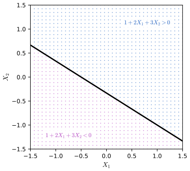
fig_9_1. Reproduces James et al. (2021), Figure 9.1. Download: PDF · SVG9.1.2 Classification Using a Separating Hyperplane
pp. 369–370 Code one class as \(y_i=+1\) (blue) and the other as \(y_i=-1\) (purple). A separating hyperplane puts every training point on its own side:
\[ y_i(\beta_0+\beta_1x_{i1}+\beta_2x_{i2}+\dots+\beta_px_{ip})>0\quad\text{for all }i=1,\dots,n, \tag{9.8} \]which is (9.6) for the blue points and (9.7) for the purple ones in one line. If one exists, classify a test point \(x^*\) by the sign of \(f(x^*)=\beta_0+\beta_1x_1^*+\dots+\beta_px_p^*\). The size of \(f(x^*)\) carries information too: by Result 9.1, \(|f(x^*)|/\|\bb\|\) is the distance to the boundary, so a large value means a confident decision. The boundary is linear.
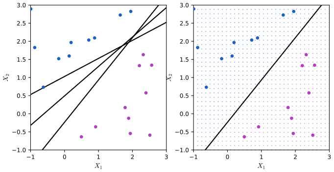
fig_9_2. Reproduces James et al. (2021), Figure 9.2. Download: PDF · SVG9.1.3 The Maximal Margin Classifier
Definition 9.2 (margin, maximal margin hyperplane, support vectors) pp. 371–372
The margin of a separating hyperplane is the smallest perpendicular distance from a training point to it. The maximal margin hyperplane (or optimal separating hyperplane) is the separating hyperplane with the largest margin: the mid-line of the widest slab that fits between the two classes. The maximal margin classifier classifies by the side of that hyperplane. The training points at distance exactly equal to the margin, on the edges of the slab, are the support vectors.
pp. 371–372 In Figure 9.3 three points are on the edges of the slab. They "support" the hyperplane: move one of them and the hyperplane moves. The other points can move freely, as long as they do not enter the slab, without changing anything (Result 9.3 says why). A large margin on the training data is hoped to mean a large margin, and few mistakes, on test data; but with many features the maximal margin classifier can overfit.
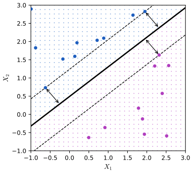
fig_9_3, hard_margin. Reproduces James et al. (2021), Figure 9.3. Download: PDF · SVG9.1.4 Construction of the Maximal Margin Classifier
pp. 372–373 The maximal margin hyperplane solves
\[ \underset{\beta_0,\beta_1,\dots,\beta_p,M}{\text{maximize}}\ M \tag{9.9} \] \[ \text{subject to}\ \sum_{j=1}^p\beta_j^2=1, \tag{9.10} \] \[ y_i(\beta_0+\beta_1x_{i1}+\beta_2x_{i2}+\dots+\beta_px_{ip})\ge M\quad\forall\,i=1,\dots,n. \tag{9.11} \]By Result 9.1(c), (9.10) makes the left side of (9.11) the distance of \(x_i\) from the hyperplane (signed by correctness), so (9.11) says that every point is on the correct side and at least \(M\) away, and (9.9) makes \(M\) as large as possible. The book stops here ("the details of this optimization are outside of the scope of this book"); the next two results are those details.
Result 9.2 (the maximal margin problem as a quadratic programme; the margin is \(1/\|\bb\|\))
If the classes are separable, (9.9)–(9.11) is equivalent to
\[ \underset{\beta_0,\bb}{\text{minimize}}\ \tfrac12\|\bb\|^2\quad\text{subject to}\quad y_i(\beta_0+\bb^\T x_i)\ge1,\ i=1,\dots,n: \]a solution \((\beta_0,\bb)\) of this problem gives the solution \((\beta_0,\bb)/\|\bb\|\), \(M=1/\|\bb\|\) of (9.9)–(9.11), and conversely. The problem is convex (a convex quadratic objective, linear constraints), so it has no local optima other than the global one, and the solution is unique. The points with \(y_i(\beta_0+\bb^\T x_i)=1\) are exactly the support vectors, and the dashed lines of Figure 9.3 are \(f(x)=+1\) and \(f(x)=-1\).
Filling the gap 9.2: from "maximise \(M\)" to "minimise \(\|\bb\|\)", and why the solution is unique p. 373
Derivation
Change of scale. In (9.9)–(9.11) the length of \(\bb\) is fixed at 1 and \(M\) is free. Instead fix the closest points at \(y_if(x_i)=1\) and let the length of \(\bb\) vary: if \((\beta_0,\bb,M)\) is feasible for (9.9)–(9.11) with \(M>0\), then \((\tilde\beta_0,\tilde\bb)=(\beta_0,\bb)/M\) satisfies \(y_i(\tilde\beta_0+\tilde\bb^\T x_i)\ge1\) and \(\|\tilde\bb\|=1/M\). Conversely, if \(y_i(\tilde\beta_0+\tilde\bb^\T x_i)\ge1\) for all \(i\), then \((\tilde\beta_0,\tilde\bb)/\|\tilde\bb\|\) with \(M=1/\|\tilde\bb\|\) is feasible for (9.9)–(9.11). So maximising \(M\) is the same as minimising \(\|\tilde\bb\|\), or \(\tfrac12\|\tilde\bb\|^2\) (squaring and halving change nothing but make the calculus clean). The width of the whole slab is \(2M=2/\|\bb\|\): the two dashed lines \(f=\pm1\) are at signed distances \(\pm1/\|\bb\|\) by Result 9.1.
Why the closest points sit at exactly 1. At the optimum some point has \(y_if(x_i)=1\); otherwise all constraints would hold with room to spare, and \(\bb\) could be shrunk a little, lowering the objective.
Uniqueness. Suppose two different solutions \((\beta_0,\bb)\) and \((\beta_0',\bb')\) both had the minimal length \(m\). Their average satisfies all the (linear) constraints, and if \(\bb\neq\bb'\) the average has length strictly less than \(m\) (the strict convexity of \(\|\cdot\|^2\): \(\|\tfrac12(\bb+\bb')\|^2=\tfrac12\|\bb\|^2+\tfrac12\|\bb'\|^2-\tfrac14\|\bb-\bb'\|^2\)), a contradiction. So \(\bb\) is unique, and \(\beta_0\) is then pinned down by the support vectors of both classes (one with \(\beta_0+\bb^\T x_i=1\), one with \(=-1\)).
When there is no solution. If no hyperplane separates the classes, the constraints \(y_if(x_i)\ge1\) have no solution, and (9.9)–(9.11) has no solution with \(M>0\): this is Section 9.1.5.
Confirmed numerically: the quadratic programme solved directly (hard_margin, scipy's SLSQP) agrees with LIBSVM run with a huge cost to five digits on the data of Figure 9.3, and \(1/\|\bb\|=0.580\) equals the smallest distance of a point to the hyperplane.
Deeper: Statistical Learning: Theory and Methods, Filling the gap 12.1 (the two forms of the problem) and Section 4.5.2 (optimal separating hyperplanes).
Result 9.3 (Lagrange multipliers: only the support vectors matter, and only inner products are needed) pp. 371–372 and 380–381, (9.17)–(9.19)
The solution of the problem of Result 9.2 can be written as
\[ \bb=\sum_{i=1}^n\alpha_iy_ix_i,\qquad \alpha_i\ge0,\qquad \sum_{i=1}^n\alpha_iy_i=0, \]with \(\alpha_i>0\) only for support vectors. Hence
\[ f(x)=\beta_0+\sum_{i\in\mathcal S}\alpha_iy_i\langle x,x_i\rangle, \]which is (9.18)–(9.19) with the book's \(\alpha_i\) equal to \(\alpha_iy_i\) here. The multipliers are found from a problem (the dual) that involves the data only through the inner products \(\langle x_i,x_{i'}\rangle\):
\[ \underset{\bal}{\text{maximize}}\ \sum_i\alpha_i-\tfrac12\sum_i\sum_{i'}\alpha_i\alpha_{i'}y_iy_{i'}\langle x_i,x_{i'}\rangle\quad\text{subject to}\quad\alpha_i\ge0,\ \sum_i\alpha_iy_i=0. \]Filling the gap 9.3: Lagrange multipliers for inequality constraints, in four steps p. 381: "it can be shown that"
Derivation
1. The Lagrangian. Attach a multiplier \(\alpha_i\ge0\) to each constraint \(y_if(x_i)-1\ge0\):
\[ L(\beta_0,\bb,\bal)=\tfrac12\|\bb\|^2-\sum_{i=1}^n\alpha_i\big[y_i(\beta_0+\bb^\T x_i)-1\big]. \]For a feasible \((\beta_0,\bb)\) every bracket is \(\ge0\), so \(\max_{\bal\ge0}L=\tfrac12\|\bb\|^2\) (take \(\bal=0\)); for an infeasible one the maximum is \(+\infty\). So the original problem is \(\min_{\beta_0,\bb}\max_{\bal\ge0}L\).
2. The conditions at the optimum (Karush–Kuhn–Tucker). For a convex problem with linear constraints, \((\beta_0,\bb)\) is optimal exactly when there are \(\alpha_i\ge0\) such that the derivatives of \(L\) in \(\beta_0\) and \(\bb\) vanish and each \(\alpha_i\) is zero unless its constraint is tight:
\[ \frac{\partial L}{\partial\bb}=\bb-\sum_i\alpha_iy_ix_i=0,\qquad \frac{\partial L}{\partial\beta_0}=-\sum_i\alpha_iy_i=0,\qquad \alpha_i\big[y_if(x_i)-1\big]=0. \]The last condition (complementary slackness) is the heart of the matter: a point strictly outside the slab has \(y_if(x_i)>1\), so its \(\alpha_i=0\) and it does not appear in \(\bb=\sum\alpha_iy_ix_i\). Moving it, without entering the slab, leaves all the conditions satisfied by the same \((\beta_0,\bb,\bal)\), so the solution does not change. This is the claim of page 371.
3. The dual. Substitute \(\bb=\sum\alpha_iy_ix_i\) and \(\sum\alpha_iy_i=0\) into \(L\): \(\tfrac12\|\bb\|^2-\bb^\T\bb+\sum\alpha_i=\sum_i\alpha_i-\tfrac12\sum_{i,i'}\alpha_i\alpha_{i'}y_iy_{i'}\langle x_i,x_{i'}\rangle\), which is maximised over \(\alpha_i\ge0\), \(\sum\alpha_iy_i=0\). Only the \(\binom n2\) inner products between pairs of points (and the \(n\) squared lengths) enter: the second bullet of page 381.
4. The intercept and new points. Any support vector has \(y_i(\beta_0+\bb^\T x_i)=1\), so \(\beta_0=y_i-\bb^\T x_i\) (LIBSVM averages this over the support vectors). For a new point, \(f(x)=\beta_0+\bb^\T x=\beta_0+\sum_i\alpha_iy_i\langle x_i,x\rangle\), which is (9.18), with nonzero terms for the support vectors only, (9.19). Footnote 2 of the book is the same identity read backwards: expanding the inner products gives back the linear function \(\beta_0+\bb^\T x\) with \(\beta_j=\sum_i\alpha_iy_ix_{ij}\).
Confirmed numerically on the Python lab's 50 points (cost 10): \(\sum_i\alpha_iy_ix_i\) equals the coefficients reported by SVC to \(10^{-10}\), \(\sum\alpha_iy_i=0\), the multipliers vanish for every point with \(y_if(x_i)>1\), and \(\beta_0+\sum_{i\in\mathcal S}\alpha_iy_i\langle x,x_i\rangle\) reproduces decision_function at new points. R's svm() stores \(\alpha_iy_i\) as coefs and the support vectors as SV, so t(coefs) %*% SV is \(\bb\) (up to the sign convention), which the lab uses to print the coefficients the book says svm() does not output.
Deeper: Statistical Learning: Theory and Methods, Result 4.16 (the dual of the optimal separating hyperplane), Result 12.1 (the Wolfe dual and strong duality) and Result 12.2 (three kinds of points); Bayesian and Probabilistic Machine Learning, Result 7.3 (KKT conditions and support vectors).
9.1.5 The Non-separable Case
p. 373 Usually no separating hyperplane exists (Figure 9.4), and then (9.9)–(9.11) has no solution with \(M>0\). The extension that tolerates some violations, with a soft margin, is the support vector classifier.
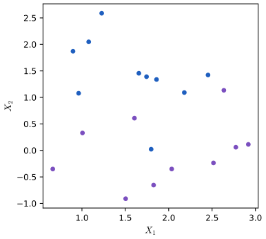
fig_9_4. Reproduces James et al. (2021), Figure 9.4. Download: PDF · SVG9.2 Support Vector Classifiers
9.2.1 Overview of the Support Vector Classifier
pp. 373–375 Even when the classes can be separated, insisting on it can be a bad idea. A classifier that must classify every training point correctly is sensitive to single observations: in Figure 9.5 one added point turns the hyperplane and cuts the margin from 0.580 to 0.215. A tiny margin means low confidence for many points, and such sensitivity is a sign of overfitting. It can pay to misclassify a few training points in exchange for robustness and better classification of the rest. The support vector classifier, or soft margin classifier, allows points on the wrong side of the margin, and if needed of the hyperplane (Figure 9.6).
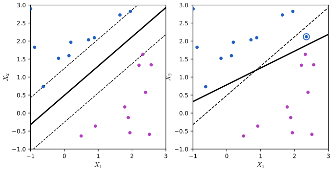
fig_9_5. Reproduces James et al. (2021), Figure 9.5. Download: PDF · SVG9.2.2 Details of the Support Vector Classifier
Definition 9.3 (support vector classifier, budget form) pp. 375–376, (9.12)–(9.15)
\[ \underset{\beta_0,\dots,\beta_p,\epsilon_1,\dots,\epsilon_n,M}{\text{maximize}}\ M \tag{9.12} \] \[ \text{subject to}\ \sum_{j=1}^p\beta_j^2=1, \tag{9.13} \] \[ y_i(\beta_0+\beta_1x_{i1}+\dots+\beta_px_{ip})\ge M(1-\epsilon_i), \tag{9.14} \] \[ \epsilon_i\ge0,\qquad\sum_{i=1}^n\epsilon_i\le C. \tag{9.15} \]The slack variable \(\epsilon_i\) says where observation \(i\) is: \(\epsilon_i=0\), on the correct side of the margin; \(0<\epsilon_i\le1\), inside the margin (it "violates the margin") but on the correct side of the hyperplane; \(\epsilon_i>1\), on the wrong side of the hyperplane. The tuning parameter \(C\ge0\) is a budget for the total violation. A test point is classified by the sign of \(f(x^*)\). The observations on the margin or on its wrong side are the support vectors; only they affect the solution.
pp. 376–377 The book's consequences of the budget: with \(C=0\) no violation is allowed and (9.12)–(9.15) is the maximal margin problem; since each point on the wrong side of the hyperplane uses more than 1 of the budget, at most \(C\) points are misclassified; and as \(C\) grows the margin widens. \(C\) is chosen by cross-validation, and it governs the bias-variance trade-off: a small budget gives a narrow margin and a fit that follows the few points near the boundary (low bias, high variance); a large budget gives a wide margin with many support vectors, a fit averaged over many points (lower variance, possibly more bias). Unlike LDA, whose rule uses every point through the class means and the pooled covariance, the support vector classifier ignores points far on the correct side of the margin; logistic regression is in between (Section 9.5).
Result 9.4 (budget, cost and penalty: three forms of one problem)
For non-separable or separable data, the following describe the same family of hyperplanes:
- the budget form (9.12)–(9.15) with budget \(C\);
- the cost form used by LIBSVM, and so by R's
svm()and scikit-learn'sSVC: \[ \underset{\beta_0,\bb,\bxi}{\text{minimize}}\ \tfrac12\|\bb\|^2+C'\sum_{i=1}^n\xi_i\quad\text{subject to}\quad y_i(\beta_0+\bb^\T x_i)\ge1-\xi_i,\ \xi_i\ge0; \] - the loss plus penalty form (9.25) of Section 9.5, with \(\lambda=1/(2C')\).
The solution \((\beta_0,\bb)\) of the cost form gives the solution of the budget form by \(M=1/\|\bb\|\), \(\epsilon_i=\xi_i=\max[0,1-y_if(x_i)]\) and \(C=\sum_i\xi_i\). The total slack \(\sum_i\xi_i\) falls as \(C'\) grows, so a large budget \(C\) is a small cost \(C'\) and a large \(\lambda\). The budget form is feasible only for \(C\) at least the smallest total hinge loss \(\min_{\beta_0,\bb}\sum_i\max[0,1-y_if(x_i)]\), which is 0 exactly for separable data.
Filling the gap 9.4: why the three forms agree, and which way the budget goes pp. 375–377, the lab on p. 389, and (9.25)
Derivation
Budget form to canonical scale. As in Filling the gap 9.2, divide \((\beta_0,\bb)\) by \(M\): (9.14) becomes \(y_i(\tilde\beta_0+\tilde\bb^\T x_i)\ge1-\epsilon_i\) with \(\|\tilde\bb\|=1/M\). So the budget form is: minimise \(\|\tilde\bb\|\) subject to \(y_if(x_i)\ge1-\epsilon_i\), \(\epsilon_i\ge0\), \(\sum\epsilon_i\le C\). The slacks are the same numbers in both scalings.
Constraint to price. This is a convex problem with one "budget" constraint. Its Lagrangian attaches a multiplier \(C'\ge0\) to \(\sum\epsilon_i\le C\): \(\tfrac12\|\bb\|^2+C'(\sum_i\epsilon_i-C)\). For the right \(C'\) (the shadow price of the budget), minimising this over the remaining constraints gives the same solution, and the constant \(-C'C\) does not matter: that is the cost form. Conversely the solution of the cost form for a given \(C'\) solves the budget form with \(C=\sum_i\xi_i\), because any hyperplane with total slack at most that \(C\) and a smaller \(\|\bb\|\) would also have a smaller cost objective.
Which way it goes. Let \(C'_1<C'_2\) with solutions \(s_1,s_2\), writing \(Q=\tfrac12\|\bb\|^2\) and \(S=\sum\xi_i\). Optimality of each gives \(Q_1+C'_1S_1\le Q_2+C'_1S_2\) and \(Q_2+C'_2S_2\le Q_1+C'_2S_1\). Adding, \((C'_2-C'_1)(S_2-S_1)\le0\), so \(S_2\le S_1\): a higher price buys less slack, and then \(Q_2\ge Q_1\), so the margin \(1/\|\bb\|\) shrinks. Large cost, small budget, narrow margin, and the reverse. The book's lab warns about exactly this: "when the cost argument is small, then the margins will be wide".
Eliminating the slacks. In the cost form, for fixed \((\beta_0,\bb)\) the best slack is the smallest one allowed, \(\xi_i=\max[0,1-y_if(x_i)]\), the hinge loss. So the cost form is \(\min\tfrac12\|\bb\|^2+C'\sum_i\max[0,1-y_if(x_i)]\); dividing by \(C'\) gives (9.25) with \(\lambda=1/(2C')\). Small \(\lambda\) is a large cost and a small budget, as the book says on page 386.
Feasibility. Every hyperplane needs total slack at least \(\sum_i\max[0,1-y_if(x_i)]\) in its canonical scaling, so budgets below the smallest total hinge loss are infeasible. On the R lab's 20 overlapping points that minimum is 4.99, and it is already reached at cost 10: every cost from about 10 upwards gives the same hyperplane, which is why the R lab's tune() reports the same error for costs 1 (nearly), 5, 10 and 100.
Confirmed numerically: on the data of Figure 9.7 with budget 4, solving (9.12)–(9.15) as written (SLSQP with \(\|\bb\|=1\)) gives the same unit \(\bb\), \(\beta_0\) and \(M=1.2037\) as LIBSVM with the matching cost 0.0936; (9.25) solved directly equals LIBSVM with cost \(1/(2\lambda)\); and along 30 costs from 0.001 to 100 the total slack falls and the margin narrows.
Deeper: Statistical Learning: Theory and Methods, Section 12.2 (the support vector classifier), Result 12.5 (the cost and penalty forms) and Section 12.3.5 (the whole path of solutions as the cost varies).
Result 9.5 (the dual of the support vector classifier: three kinds of points)
The cost form has the same dual as Result 9.3 except that each multiplier is capped: \(0\le\alpha_i\le C'\). At the solution, \(\alpha_i=0\) for points beyond the margin (\(y_if(x_i)>1\)), \(0<\alpha_i<C'\) only for points exactly on the margin (\(y_if(x_i)=1\)), and \(\alpha_i=C'\) for points inside the margin or misclassified (\(y_if(x_i)<1\)). Still \(\bb=\sum\alpha_iy_ix_i\) and \(f(x)=\beta_0+\sum_{i\in\mathcal S}\alpha_iy_i\langle x,x_i\rangle\).
Filling the gap 9.5: where the cap \(\alpha_i\le C'\) comes from p. 377
Derivation
The Lagrangian of the cost form has multipliers \(\alpha_i\ge0\) for \(y_if(x_i)\ge1-\xi_i\) and \(\mu_i\ge0\) for \(\xi_i\ge0\): \(\tfrac12\|\bb\|^2+C'\sum\xi_i-\sum\alpha_i[y_if(x_i)-1+\xi_i]-\sum\mu_i\xi_i\). Setting the derivative in \(\xi_i\) to zero gives \(C'-\alpha_i-\mu_i=0\), so \(\alpha_i=C'-\mu_i\le C'\). The derivatives in \(\bb\) and \(\beta_0\) are as before. Complementary slackness now has two parts: \(\alpha_i[y_if(x_i)-1+\xi_i]=0\) and \(\mu_i\xi_i=0\). If \(y_if(x_i)>1\), then \(\xi_i=0\) and the first bracket is positive, so \(\alpha_i=0\). If \(0<\alpha_i<C'\), then \(\mu_i>0\), so \(\xi_i=0\), and the first bracket must vanish: \(y_if(x_i)=1\). If \(y_if(x_i)<1\), then \(\xi_i>0\), so \(\mu_i=0\) and \(\alpha_i=C'\). Substituting back, the \(\xi_i\) and \(\mu_i\) cancel and the dual objective is unchanged, with the box \(0\le\alpha_i\le C'\).
The support vectors are therefore the points on the margin or on its wrong side, as the book says, and each misclassified point pulls with the same maximal force \(C'\), however far it is: one reason the support vector classifier is robust to outlying points on the correct side and does not let a single misclassified point dominate. Confirmed numerically on the Python lab's data with cost 10: the 21 points with \(y_if>1\) have \(\alpha_i=0\), the three free multipliers sit at \(y_if=1\), and the 26 points with \(\alpha_i=10\) all have \(y_if\le1\).
Algorithm 9.1 (how LIBSVM solves the dual: sequential minimal optimisation)
- Start from \(\bal=0\) (feasible). Keep the gradient \(G_i=y_i\sum_{i'}\alpha_{i'}y_{i'}K_{ii'}-1\) of the dual objective (written as a minimisation).
- Pick the pair \((i,j)\) that most violates the optimality conditions (LIBSVM uses a second-order rule). Two multipliers is the smallest number that can move while keeping \(\sum\alpha_iy_i=0\).
- Minimise the dual exactly along the line in \((\alpha_i,\alpha_j)\) that keeps \(\sum\alpha_iy_i\) fixed, a one-dimensional quadratic; clip the step to the box \([0,C']\).
- Update \(G\) (two kernel columns) and repeat until the largest violation is below a tolerance (0.001 by default in both R and Python). Then set \(\beta_0\) from the points on the margin.
The three demonstrations of this chapter run this algorithm in the browser. Because R's e1071 and Python's sklearn.svm both call LIBSVM, they agree to all printed digits when given the same data, in the same row order, with the same scaling.
See also: Bayesian and Probabilistic Machine Learning, Algorithm 7.1 (from chunking to SMO) and Filling the gap 7.3 (the analytic two-multiplier step).
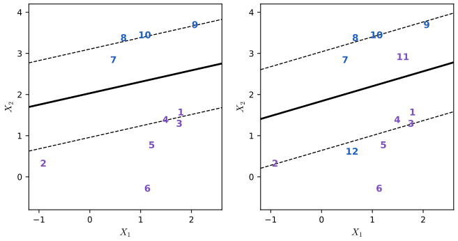
fig_9_6. Reproduces James et al. (2021), Figure 9.6. Download: PDF · SVG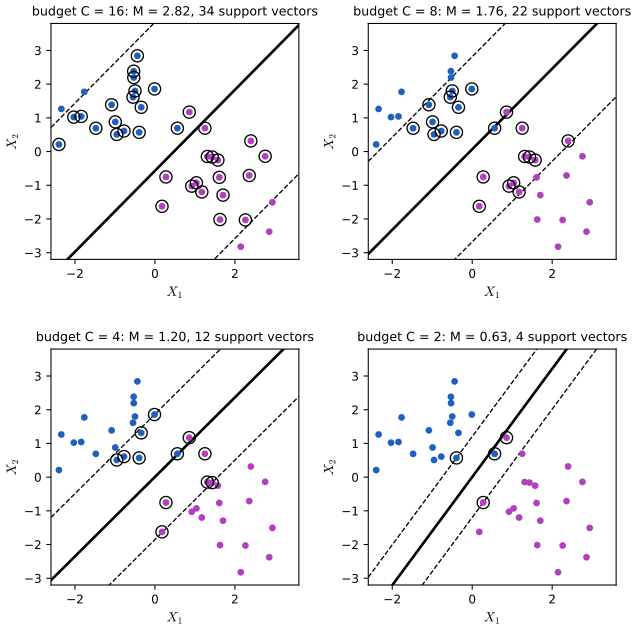
fig_9_7, budget_fit. Reproduces James et al. (2021), Figure 9.7. Download: PDF · SVG9.3 Support Vector Machines
9.3.1 Classification with Non-Linear Decision Boundaries
pp. 379–380 When the classes are arranged as in Figure 9.8 (one class in the middle, the other at both ends), every linear boundary fails. As with regression in Chapter 7, one remedy is to enlarge the feature space: fit the support vector classifier on \(X_1,X_1^2,X_2,X_2^2,\dots,X_p,X_p^2\), that is
\[ \underset{\beta_0,\beta_{11},\beta_{12},\dots,\beta_{p1},\beta_{p2},\epsilon_1,\dots,\epsilon_n,M}{\text{maximize}}\ M\quad\text{subject to}\quad y_i\Big(\beta_0+\sum_{j=1}^p\beta_{j1}x_{ij}+\sum_{j=1}^p\beta_{j2}x_{ij}^2\Big)\ge M(1-\epsilon_i), \tag{9.16} \]with \(\sum_i\epsilon_i\le C\), \(\epsilon_i\ge0\) and \(\sum_j\sum_k\beta_{jk}^2=1\). The boundary is linear in the enlarged space but a quadratic curve \(q(x)=0\) in the original one. Higher powers and interactions \(X_jX_{j'}\) give still more flexible boundaries, but the number of features grows quickly (Filling the gap 9.6).
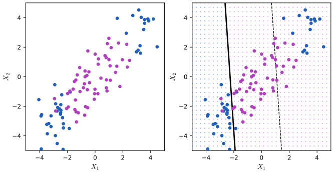
fig_9_8. Reproduces James et al. (2021), Figure 9.8. Download: PDF · SVG9.3.2 The Support Vector Machine
pp. 380–383 By Result 9.3 the support vector classifier needs the data only through inner products (9.17): to fit it (the dual) and to evaluate it, (9.18)–(9.19). Now replace every inner product by a kernel \(K(x_i,x_{i'})\) (9.20), a function measuring the similarity of two observations. The linear kernel (9.21) \(K(x_i,x_{i'})=\sum_jx_{ij}x_{i'j}\) gives back the support vector classifier. Two other common choices are
\[ K(x_i,x_{i'})=\Big(1+\sum_{j=1}^px_{ij}x_{i'j}\Big)^d \qquad\text{(polynomial kernel of degree }d\text{)}, \tag{9.22} \] \[ K(x_i,x_{i'})=\exp\Big(-\gamma\sum_{j=1}^p(x_{ij}-x_{i'j})^2\Big) \qquad\text{(radial kernel, }\gamma>0\text{)}. \tag{9.24} \]The resulting classifier, the support vector machine, has the form
\[ f(x)=\beta_0+\sum_{i\in\mathcal S}\alpha_iK(x,x_i). \tag{9.23} \]The radial kernel is local: if \(x^*\) is far from \(x_i\), \(K(x^*,x_i)\) is tiny and \(x_i\) plays essentially no part in \(f(x^*)\). So \(f\) is a sum of bumps centred at the support vectors, with width about \(1/\sqrt\gamma\). Kernels also save computation: we only need the \(\binom n2\) values \(K(x_i,x_{i'})\), never the enlarged features, and for the radial kernel the feature space is infinite-dimensional, so there would be no other way.
Definition 9.4 (kernel)
A kernel is a function \(K(x,z)\) for which there is a map \(\bphi\) from \(\R^p\) to some (possibly infinite-dimensional) space with \(K(x,z)=\langle\bphi(x),\bphi(z)\rangle\). Equivalently (Mercer's condition), \(K\) is symmetric and every Gram matrix \(\bK=[K(x_i,x_{i'})]\) built from any finite set of points is positive semi-definite.
Result 9.6 (what a kernel computes)
(a) For \(p=2\) and \(d=2\), \((1+\langle x,z\rangle)^2=\bphi(x)^\T\bphi(z)\) with \(\bphi(x)=(1,\sqrt2x_1,\sqrt2x_2,x_1^2,x_2^2,\sqrt2x_1x_2)\): the polynomial kernel is the support vector classifier on all monomials of degree at most 2, with particular weights. In general the degree-\(d\) polynomial kernel corresponds to the \(\binom{p+d}{d}\) monomials of degree at most \(d\). (b) The radial kernel corresponds to infinitely many features. (c) Running the support vector classifier with \(K\) in place of the inner product is the support vector classifier in the space of \(\bphi(x)\): the boundary \(f(x)=0\) is a hyperplane there, and a curve or surface in \(\R^p\).
Filling the gap 9.6: the hidden features of the polynomial and radial kernels, and why the kernel must be positive semi-definite pp. 382–383: "it essentially amounts to fitting a support vector classifier in a higher-dimensional space"
Derivation
Polynomial kernel. \((1+x_1z_1+x_2z_2)^2=1+2x_1z_1+2x_2z_2+x_1^2z_1^2+x_2^2z_2^2+2x_1x_2z_1z_2\), which is \(\bphi(x)^\T\bphi(z)\) for the six features of (a). In general, the multinomial theorem expands \((1+\sum_jx_jz_j)^d\) into one term for every monomial \(x_1^{k_1}\cdots x_p^{k_p}\) with \(k_1+\dots+k_p\le d\), times the same monomial of \(z\), times a positive multinomial coefficient; the number of such monomials is \(\binom{p+d}{d}\). For the 16 columns of the Heart data and \(d=3\) that is 969 features, while the kernel costs one inner product and a cube.
Radial kernel. In one dimension, \(e^{-\gamma(x-z)^2}=e^{-\gamma x^2}e^{-\gamma z^2}e^{2\gamma xz}\) and \(e^{2\gamma xz}=\sum_{k\ge0}\frac{(2\gamma)^k}{k!}x^kz^k\), so \(K(x,z)=\sum_k\phi_k(x)\phi_k(z)\) with \(\phi_k(x)=e^{-\gamma x^2}\sqrt{(2\gamma)^k/k!}\,x^k\), \(k=0,1,2,\dots\): infinitely many features, every power of \(x\) damped by a Gaussian. In \(p\) dimensions the kernel is a product of such factors.
Why it works. Replace \(x_i\) by \(\bphi(x_i)\) in Filling the gap 9.3: the derivation never used anything but inner products, so the dual and \(f(x)=\beta_0+\sum\alpha_iy_i\langle\bphi(x),\bphi(x_i)\rangle\) need only \(K\). The coefficient vector \(\bb=\sum\alpha_iy_i\bphi(x_i)\) lives in the feature space and is never formed.
Why positive semi-definite. The dual objective contains \(\tfrac12\sum\alpha_i\alpha_{i'}y_iy_{i'}K(x_i,x_{i'})\), a quadratic form in the vector \((\alpha_iy_i)\) with matrix \(\bK\). If \(\bK\) is positive semi-definite the dual is a concave maximisation with a global solution that the algorithm finds; if not, the problem can be unbounded and "the" solution meaningless. A Gram matrix of genuine inner products is always positive semi-definite, since \(\sum_{i,i'}c_ic_{i'}\langle\bphi(x_i),\bphi(x_{i'})\rangle=\|\sum_ic_i\bphi(x_i)\|^2\ge0\). Not every similarity measure qualifies; the sigmoid kernel \(\tanh(a\langle x,z\rangle+b)\) offered by both svm() and SVC, for example, is not positive semi-definite for all settings.
The scale of \(\gamma\). \(\gamma\) multiplies a squared distance, so its meaning depends on the units of the features: standardising them first (R's svm() does this by default, SVC does not) changes what a given \(\gamma\) does. In the radial fit the support vectors are the points near or across the boundary, and each contributes a bump of height \(\alpha_iy_i\).
Confirmed numerically: the feature-map identity for random points, \(\binom{19}{3}=969\), the series for the radial kernel, and that the radial Gram matrices of the 297 Heart patients (\(\gamma=0.01,0.1,1\)) have no negative eigenvalues.
Deeper: Statistical Learning: Theory and Methods, Section 12.3, Result 12.4 (the kernel trick and the polynomial kernel's features), Section 12.3.3 (reproducing kernels) and Section 12.3.4 (SVMs and the curse of dimensionality).
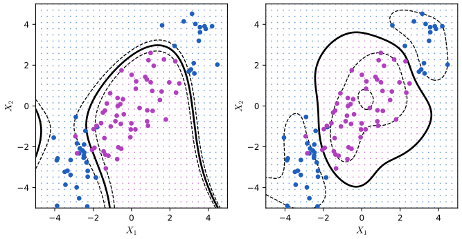
fig_9_9. Reproduces James et al. (2021), Figure 9.9. Download: PDF · SVG9.3.3 An Application to the Heart Disease Data
pp. 383–384 The Heart data record 13 predictors (age, sex, cholesterol, chest pain type, and so on) and whether each of 303 patients has heart disease; removing 6 with missing values leaves 297. The book splits them at random into 207 training and 90 test patients and compares LDA, the support vector classifier and radial SVMs by ROC curves (Chapter 4). Each method produces a score \(\hat f(X)\); predicting disease when \(\hat f(X)\ge t\) and moving \(t\) traces the curve. On the training data (Figure 9.10) the curves improve as \(\gamma\) grows, and \(\gamma=0.1\) is nearly perfect; on the test data (Figure 9.11) \(\gamma=0.1\) is the worst. The book's split is not published; our split is one draw (default_rng(1)) with the 16 columns standardised, so the curves differ in detail, but the pattern is the book's.
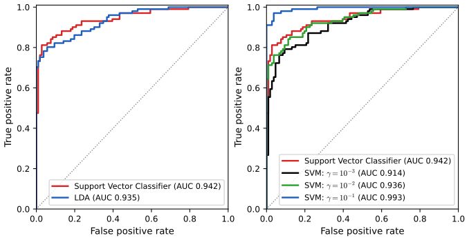
fig_9_10, heart_data, roc_points. Reproduces James et al. (2021), Figure 9.10. Download: PDF · SVG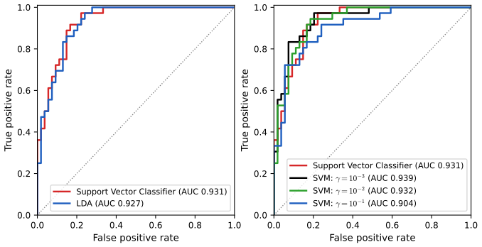
fig_9_11. Reproduces James et al. (2021), Figure 9.11. Download: PDF · SVGTwo facts make these curves easy to read. The ROC curve depends only on the ordering of the scores, so any increasing transformation of \(\hat f\) gives the same curve, and the area under it is the probability that a randomly chosen patient with disease scores higher than a randomly chosen one without (Chapter 4, Result 4.4). And an SVM score is not a probability: \(\hat f(x)\) is a signed distance in the feature space, useful for ranking and thresholding, but it needs an extra calibration step (for example a logistic regression of \(y\) on \(\hat f\), Platt scaling) before it can be read as \(\Pr(Y=1\given x)\).
See also: Bayesian and Probabilistic Machine Learning, Filling the gap 7.4 (why the SVM gives no probabilities).
9.4 SVMs with More than Two Classes
p. 385 A hyperplane has two sides, so SVMs are built for two classes. The two common extensions combine binary SVMs.
9.4.1 One-Versus-One Classification
9.4.2 One-Versus-All Classification
Algorithm 9.2 (one-versus-one and one-versus-all) pp. 385–386
One-versus-one (all pairs). For each of the \(\binom K2\) pairs of classes \((k,k')\), fit an SVM on the observations of those two classes only. Classify \(x^*\) with each of them and count how often each class wins; predict the class with the most votes.
One-versus-all (one-versus-rest). For each class \(k\), fit an SVM of class \(k\) (coded \(+1\)) against all the others (\(-1\)), with function \(f_k(x)=\beta_{0k}+\beta_{1k}x_1+\dots+\beta_{pk}x_p\). Predict the class with the largest \(f_k(x^*)\).
Filling the gap 9.7: counting, ties, and what the software actually does pp. 385–386, and the labs (pp. 396 and 393)
Derivation
Size. One-versus-one fits \(K(K-1)/2\) classifiers, each on about \(2n/K\) observations; one-versus-all fits \(K\), each on all \(n\). Since SVM training grows faster than linearly in \(n\), many small problems are often cheaper than a few large ones, one reason LIBSVM uses one-versus-one. One-versus-all has an imbalance problem (one class against \(K-1\)) and compares scores \(f_k\) from different fits, whose scales need not match; one-versus-one can end in a tie in the vote, which LIBSVM breaks in favour of the class listed first.
What the software does. R's svm() always uses one-versus-one. So does scikit-learn's SVC: its decision_function_shape="ovr" option only rearranges the one-versus-one votes into an \(n\times K\) table; it does not fit \(K\) one-versus-all classifiers (see the notes on the book). A true one-versus-all fit takes OneVsRestClassifier(SVC(...)) in Python and a loop over classes in R; both are in the lab.
Confirmed numerically: on the Khan data SVC returns \(\binom42=6\) decision columns, and counting their votes by hand reproduces predict(); fits with "ovo" and "ovr" have identical support vectors and coefficients.
See also: Bayesian and Probabilistic Machine Learning, Section 7.1.3 (multiclass SVMs, and their inconsistencies).
9.5 Relationship to Logistic Regression
pp. 386–388 The support vector classifier can be written as
\[ \underset{\beta_0,\beta_1,\dots,\beta_p}{\text{minimize}}\ \left\{\sum_{i=1}^n\max\big[0,1-y_if(x_i)\big]+\lambda\sum_{j=1}^p\beta_j^2\right\}, \tag{9.25} \]with \(\lambda\ge0\) (Result 9.4). It is of the "loss plus penalty" form
\[ \underset{\beta_0,\beta_1,\dots,\beta_p}{\text{minimize}}\ \big\{L(\bX,\by,\bb)+\lambda P(\bb)\big\} \tag{9.26} \]met throughout the book: ridge regression and the lasso have the squared-error loss with \(P(\bb)=\sum\beta_j^2\) or \(\sum|\beta_j|\); here the penalty is ridge's and the loss is the hinge loss \(\sum_i\max[0,1-y_i(\beta_0+\beta_1x_{i1}+\dots+\beta_px_{ip})]\). Large \(\lambda\): small \(\beta_j\), many violations, low variance and high bias; small \(\lambda\): the reverse, so a small \(\lambda\) is a small budget \(C\). The tuning parameter matters a great deal, contrary to the early view of it as a nuisance to be set at 1. In this scaling the margin corresponds to \(y_if(x_i)=1\) and its width is governed by \(\sum\beta_j^2\) (the book's footnote 3).
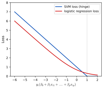
fig_9_12. Reproduces James et al. (2021), Figure 9.12. Download: PDF · SVGPoints on the correct side of the margin have zero hinge loss, and that is why they do not affect the support vector classifier. The logistic loss is never zero, but tiny for points far from the boundary, so logistic regression and the support vector classifier usually give similar answers; with well separated classes SVMs tend to do better, with overlapping classes logistic regression is often preferred. Nor are kernels special to SVMs: logistic regression could use them as well, closely related to the non-linear methods of Chapter 7; their use with SVMs is mainly historical.
Result 9.7 (the logistic loss, the slopes of the losses, and what each loss estimates)
(a) With \(y\in\{-1,+1\}\) and \(\Pr(Y=1\given x)=e^{f(x)}/(1+e^{f(x)})\), the negative log-likelihood of one observation is \(\log(1+e^{-yf(x)})\): logistic regression minimises the logistic loss, and the logistic analogue of (9.25) is ridge-penalised logistic regression. (b) In the equations that define the fit, observation \(i\) enters with weight equal to minus the slope of its loss at \(y_if(x_i)\): for the hinge, 1 inside the margin and 0 beyond it; for the logistic loss, \(1-\Pr(\text{correct class}\given x_i)\), never 0. (c) If \(p(x)=\Pr(Y=1\given x)\), the expected hinge loss is minimised by \(f(x)=\sign[p(x)-\tfrac12]\), the Bayes classifier, while the expected logistic loss is minimised by \(f(x)=\log[p(x)/(1-p(x))]\), the log-odds. (d) Both losses, the logistic one divided by \(\log2\), are convex upper bounds of the 0-1 loss \(I(yf\le0)\).
Filling the gap 9.8: the two losses side by side pp. 386–388: "it turns out that the hinge loss function is closely related to the loss function used in logistic regression"
Derivation
(a) For \(y=+1\) the likelihood contribution is \(p=1/(1+e^{-f})\), so \(-\log p=\log(1+e^{-f})\); for \(y=-1\) it is \(1-p=1/(1+e^{f})\), so \(-\log(1-p)=\log(1+e^{f})\). Both are \(\log(1+e^{-yf})\). This is the log-likelihood of Chapter 4, Result 4.1 with the labels coded \(\pm1\) instead of 0/1.
(b) Setting the derivative of \(\sum_i\ell(y_if(x_i))+\lambda\|\bb\|^2\) with respect to \(\bb\) to zero gives \(2\lambda\bb=\sum_i[-\ell'(y_if(x_i))]\,y_ix_i\). For the logistic loss \(-\ell'(m)=1/(1+e^{m})\), which at \(m=y_if(x_i)\) is \(1-\Pr(Y=y_i\given x_i)\). For the hinge, \(-\ell'(m)\) is 1 for \(m<1\) and 0 for \(m>1\), with anything in \([0,1]\) allowed at \(m=1\); comparing with \(\bb=\sum\alpha_iy_ix_i\), the weights are \(\alpha_i/C'\), the multipliers of Result 9.5. So \(\bb\) is a weighted sum of the \(y_ix_i\) in both methods; the hinge gives the far points weight exactly 0, the logistic loss a small positive weight.
(c) At a fixed \(x\) the expected hinge loss is \(R(f)=p\max(0,1-f)+(1-p)\max(0,1+f)\). On \([-1,1]\) it is \(p(1-f)+(1-p)(1+f)=1+(1-2p)f\), linear in \(f\), so the minimum is at \(f=1\) if \(p>\tfrac12\) and at \(f=-1\) if \(p<\tfrac12\); outside \([-1,1]\) \(R\) only increases. The minimiser is \(\sign(2p-1)\): the hinge estimates the Bayes decision and nothing more, which is why SVM scores are not probabilities. For the logistic loss \(R(f)=p\log(1+e^{-f})+(1-p)\log(1+e^{f})\) has derivative \(-p/(1+e^{f})+(1-p)e^{f}/(1+e^{f})\), zero when \(e^f=p/(1-p)\): the log-odds, from which probabilities follow.
(d) If \(m=yf\le0\), then \(\max(0,1-m)\ge1\) and \(\log(1+e^{-m})\ge\log2\). Convexity is what makes both problems solvable to their global minimum; the 0-1 loss itself is neither convex nor continuous.
Support vector regression (page 388) applies the same idea to a numerical response: the loss \(\max(0,|y-f(x)|-\epsilon)\) ignores residuals smaller than \(\epsilon\), so the points inside a tube of half-width \(\epsilon\) around the fit are not support vectors.
Confirmed numerically: the identities of (a) and (d) on a grid, and the minimisers of (c) for \(p=0.2,0.45,0.7,0.9\) by brute force. In the demonstration, pushing the well-classified points of the Python lab's data further away leaves the support vector classifier exactly unchanged and moves the logistic boundary.
Deeper: Statistical Learning: Theory and Methods, Section 12.3.2 (the SVM as a penalisation method), Result 12.6 (the population minimisers of the losses) and Section 12.3.6 (support vector regression); Bayesian and Probabilistic Machine Learning, Result 7.8.
9.6 Lab: Support Vector Machines
p. 388 The R lab of James et al. 2021 uses svm() and tune() from the e1071 package and ROCR for ROC curves; the Python lab of James et al. 2023 uses scikit-learn's SVC, GridSearchCV and RocCurveDisplay, with plotting helpers from the authors' own package. Both svm() and SVC call the LIBSVM library. Here the R version follows the R lab with its seeds, and the Python version follows the Python lab with its seeds, written with numpy, pandas, matplotlib and scikit-learn only; so each reproduces the printed numbers of its own edition. Because the two editions simulate different data, the Python file also refits the R lab's data (exported by the R script) and gets the R lab's answers. The complete files are code/ch09_lab.R and code/ch09_lab.py; the excerpts below are taken from them verbatim, except that lines which only record a number in cache/, export data or open and close a graphics file are left out.
Where the two languages differ, and why
- Different data. R's
set.seed(1); rnorm(...)and numpy'sdefault_rng(1)produce different numbers, and the editions simulate different sizes (20 and 50 points in Section 9.6.1). On the same data the two give identical fits: Python'sSVCon the R lab's 20 points finds R's support vectors 1, 2, 5, 7, 14, 16, 17 and \(\bb=(1.5555,1.6115)\), \(\beta_0=-1.5067\); R's tables, support-vector counts and ROC areas are all reproduced. - Scaling.
svm()standardises every feature by default (scale = TRUE, mean 0 and standard deviation 1 with divisor \(n-1\), from the training data);SVCdoes not. The R lab turns scaling off in its first fits but leaves it on for the separable data, the radial kernels and the Khan data. So "\(\gamma=1\)" in the R lab and in the Python lab are different kernels. To reproduce an R fit in Python, standardise first (e1071_scalebelow). - Cross-validation.
tune()uses 10 random folds,GridSearchCVhere 5 shuffled folds; their error estimates differ, and ties between grid points are broken differently. The exercises use folds fixed by row number in both languages, so their numbers agree exactly. - Signs and order. LIBSVM orients \(f\) so that \(f>0\) predicts the class it met first in the data: \(-1\) in the R lab (hence the R lab's
-fittedin ROC curves), the larger label inSVC, which sorts the classes. The row order of the training data can change the last digits of a fit, and with them ties in ROC rankings; the Python refit uses R'ssample()order to match R exactly. - Output.
svm()does not print \(\bb\) or the margin; they follow fromcoefsandSV(Result 9.3).SVChascoef_for the linear kernel.
9.6.1 Support Vector Classifier
Setup and helpers. R loads e1071 and ROCR; Python needs a confusion table, the coefficients of a linear fit from its dual solution, a plotting function and the scaling of svm().
R
suppressPackageStartupMessages({
  library(ISLR2)
  library(e1071)
  library(ROCR)
})
options(digits = 6, width = 100)
Python
def confusion_table(predicted, truth):
    """Counts of (predicted, true) labels, predicted classes in the rows."""
    return pd.crosstab(pd.Series(predicted, name="Predicted"), pd.Series(truth, name="Truth"))

def linear_coefficients(model):
    """beta_0 and beta of a fitted linear SVC from its dual solution: beta = sum_i (alpha_i y_i) x_i,
    the representation (9.18)-(9.19); dual_coef_ holds alpha_i y_i for the support vectors."""
    beta = (model.dual_coef_ @ model.support_vectors_).ravel()
    return model.intercept_[0], beta

def e1071_scale(Xtrain):
    """The scaling e1071::svm() applies by default (scale = TRUE): centre and divide by the standard
    deviation (divisor n - 1) of the training data; returns a function applying it to any rows."""
    m, s = Xtrain.mean(0), Xtrain.std(0, ddof=1)
    return lambda Z: (np.asarray(Z, float) - m) / s
The plotting helpers: plot_fit (R) and plot_svm (Python)
R
plot_fit <- function(fit, x, y, main = "", pal = c("#7b4fbf", "#1f5fbf", "#2ca02c")) {
  g1 <- seq(min(x[, 1]) - 0.5, max(x[, 1]) + 0.5, length.out = 200)
  g2 <- seq(min(x[, 2]) - 0.5, max(x[, 2]) + 0.5, length.out = 200)
  G <- expand.grid(x.1 = g1, x.2 = g2)
  pr <- predict(fit, G, decision.values = TRUE)
  cls <- matrix(as.integer(pr), length(g1))
  image(g1, g2, cls, col = adjustcolor(pal[seq_along(levels(y))], 0.15),
        xlab = "x.1", ylab = "x.2", main = main, useRaster = TRUE)
  if (nlevels(y) == 2) contour(g1, g2, matrix(attr(pr, "decision.values"), length(g1)), levels = c(-1, 0, 1),
                               lty = c(2, 1, 2), drawlabels = FALSE, add = TRUE)
  col <- pal[as.integer(y)]
  sv <- seq_len(nrow(x)) %in% fit$index
  points(x[!sv, ], col = col[!sv], pch = 19, cex = 0.8)
  points(x[sv, ], col = col[sv], pch = 3, cex = 1.3, lwd = 2)
}
Python
def plot_svm(X, y, model, ax, title=None, colours=("#7b4fbf", "#1f5fbf", "#2ca02c")):
    """Shade the predicted class over a grid, draw the margins of a two-class fit (f = -1, 0, 1)
    and mark the support vectors with a plus sign."""
    lo, hi = X.min(0) - 0.5, X.max(0) + 0.5
    g1, g2 = np.meshgrid(np.linspace(lo[0], hi[0], 300), np.linspace(lo[1], hi[1], 300))
    G = np.column_stack([g1.ravel(), g2.ravel()])
    classes = list(model.classes_)
    pred = np.searchsorted(classes, model.predict(G)).reshape(g1.shape)
    from matplotlib.colors import ListedColormap
    cmap = ListedColormap([c for c in colours[:len(classes)]])
    ax.contourf(g1, g2, pred, levels=np.arange(len(classes) + 1) - 0.5, cmap=cmap, alpha=0.12)
    if len(classes) == 2:
        f = model.decision_function(G).reshape(g1.shape)
        ax.contour(g1, g2, f, levels=[-1, 0, 1], colors="k", linestyles=["--", "-", "--"], linewidths=[1, 1.5, 1])
    sv = np.zeros(len(y), bool)
    sv[model.support_] = True
    for k, c in enumerate(classes):
        m = (np.asarray(y) == c)
        ax.scatter(X[m & ~sv, 0], X[m & ~sv, 1], s=22, color=colours[k], edgecolors="none")
        ax.scatter(X[m & sv, 0], X[m & sv, 1], s=60, color=colours[k], marker="+", linewidths=1.6)
    ax.set(xlabel="$X_1$", ylabel="$X_2$", title=title)
Two overlapping classes and a linear fit. The R lab simulates 20 points, the Python lab 50; class \(+1\) is shifted by 1 in each coordinate, so the classes overlap.
R
set.seed(1)
x <- matrix(rnorm(20 * 2), ncol = 2)
y <- c(rep(-1, 10), rep(1, 10))
x[y == 1, ] <- x[y == 1, ] + 1
dat <- data.frame(x = x, y = as.factor(y))

svmfit <- svm(y ~ ., data = dat, kernel = "linear", cost = 10, scale = FALSE)
print(svmfit$index)
summary(svmfit)
b10 <- drop(t(svmfit$coefs) %*% svmfit$SV)              # what svm() does not print: beta ...
cat("beta =", -b10, " beta_0 =", svmfit$rho, " margin 1/||beta|| =", 1 / sqrt(sum(b10^2)), "\n")
svmfit01 <- svm(y ~ ., data = dat, kernel = "linear", cost = 0.1, scale = FALSE)
print(svmfit01$index)
plot_fit(svmfit, x, dat$y, "cost = 10"); plot_fit(svmfit01, x, dat$y, "cost = 0.1")
Python
rng = np.random.default_rng(1)
X = rng.standard_normal((50, 2))
y = np.array([-1] * 25 + [1] * 25)
X[y == 1] += 1                                  # the classes overlap: not linearly separable

svm_linear = SVC(C=10, kernel="linear").fit(X, y)
svm_linear_small = SVC(C=0.1, kernel="linear").fit(X, y)
b0, beta = linear_coefficients(svm_linear)
print("C = 10:  beta =", beta, " beta_0 = %.4f" % b0, " coef_ =", svm_linear.coef_.ravel())
print("support vectors per class: C = 10", svm_linear.n_support_, "  C = 0.1", svm_linear_small.n_support_)
print("margin 1/||beta||: C = 10 %.4f,  C = 0.1 %.4f" % (1 / np.linalg.norm(beta),
                                                      1 / np.linalg.norm(linear_coefficients(svm_linear_small)[1])))

fig, ax = plt.subplots(1, 2, figsize=(9, 4.3))
plot_svm(X, y, svm_linear, ax[0], "C = 10")
plot_svm(X, y, svm_linear_small, ax[1], "C = 0.1")
common.savefig(fig, 9, "lab-py-svc", formats=("svg",))
[1] 1 2 5 7 14 16 17 Number of Support Vectors: 7 ( 4 3 ) beta = 1.55555 1.61153 beta_0 = -1.50671 margin 1/||beta|| = 0.446466 [1] 1 2 3 4 5 7 9 10 12 13 14 15 16 17 18 20
C = 10:  beta = [1.173  0.7735]  beta_0 = -0.8199  coef_ = [1.173  0.7735]
support vectors per class: C = 10 [15 14]   C = 0.1 [18 18]
margin 1/||beta||: C = 10 0.7117,  C = 0.1 1.1801
Both labs make the book's point: a smaller cost (a larger budget) widens the margin and adds support vectors (7 to 16 in R, 29 to 36 in Python). The coefficients computed from the dual solution are exactly coef_; in R they are the coefficients the book says svm() does not output. In Python the margin \(1/\|\bb\|\) grows from 0.71 at \(C=10\) to 1.18 at \(C=0.1\).
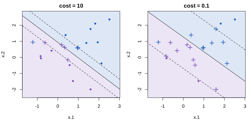
lab-r-svc.svg, made by ch09_lab.R.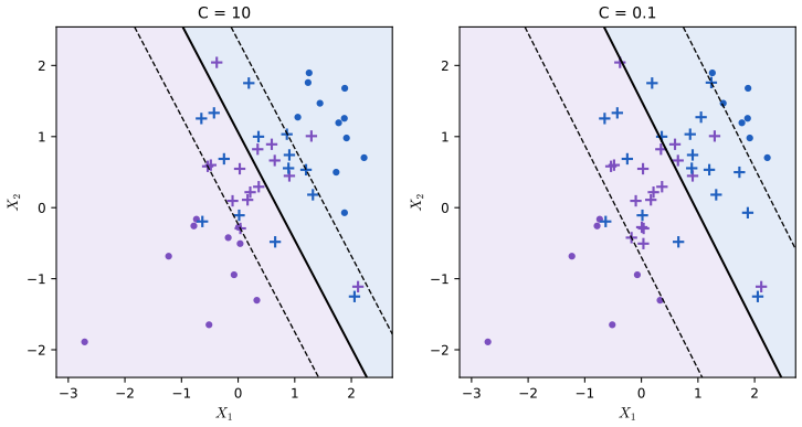
lab-py-svc.svg, made by ch09_lab.py.Choosing the cost by cross-validation, and predicting new points.
R
set.seed(1)
tune.out <- tune(svm, y ~ ., data = dat, kernel = "linear",
                 ranges = list(cost = c(0.001, 0.01, 0.1, 1, 5, 10, 100)))
summary(tune.out)
bestmod <- tune.out$best.model

xtest <- matrix(rnorm(20 * 2), ncol = 2)
ytest <- sample(c(-1, 1), 20, rep = TRUE)
xtest[ytest == 1, ] <- xtest[ytest == 1, ] + 1
testdat <- data.frame(x = xtest, y = as.factor(ytest))
ypred <- predict(bestmod, testdat)
print(table(predict = ypred, truth = testdat$y))
svmfit <- svm(y ~ ., data = dat, kernel = "linear", cost = .01, scale = FALSE)
ypred01 <- predict(svmfit, testdat)
print(table(predict = ypred01, truth = testdat$y))
Python
kfold = skm.KFold(5, random_state=0, shuffle=True)
grid = skm.GridSearchCV(svm_linear, {"C": [0.001, 0.01, 0.1, 1, 5, 10, 100]},
                        refit=True, cv=kfold, scoring="accuracy").fit(X, y)
print("best C:", grid.best_params_, " CV accuracy:", grid.cv_results_["mean_test_score"])

X_test = rng.standard_normal((20, 2))
y_test = np.array([-1] * 10 + [1] * 10)
X_test[y_test == 1] += 1
best_ = grid.best_estimator_
print(confusion_table(best_.predict(X_test), y_test))
svm_ = SVC(C=0.001, kernel="linear").fit(X, y)
print(confusion_table(svm_.predict(X_test), y_test))
- best parameters:
cost
0.1
cost error dispersion
1 1e-03 0.55 0.437798
2 1e-02 0.55 0.437798
3 1e-01 0.05 0.158114
4 1e+00 0.15 0.241523
5 5e+00 0.15 0.241523
6 1e+01 0.15 0.241523
7 1e+02 0.15 0.241523
truth
predict -1 1
-1 9 1
1 2 8
truth
predict -1 1
-1 11 6
1 0 3best C: {'C': 1} CV accuracy: [0.46 0.46 0.72 0.74 0.74 0.74 0.74]
Truth -1 1
Predicted
-1 8 4
1 2 6
Truth -1 1
Predicted
-1 2 0
1 8 10R: cost 0.1 has the smallest ten-fold error (0.05), and its fit classifies 17 of the 20 test points correctly; cost 0.01 only 14. Python: \(C=1\) has the highest five-fold accuracy (0.74, tied with larger values, and GridSearchCV takes the first) and 70% test accuracy; \(C=0.001\) gets 60%. The identical errors for costs from 1 to 100 are not a coincidence: on overlapping data the fit stops changing once the cost is large enough (Filling the gap 9.4).
Barely separable classes. Shifting class \(+1\) further makes the classes separable; a huge cost then gives (nearly) the maximal margin classifier, a small one a wider soft margin.
R
x[y == 1, ] <- x[y == 1, ] + 0.5                       # now the classes are barely separable
dat <- data.frame(x = x, y = as.factor(y))
svmfit <- svm(y ~ ., data = dat, kernel = "linear", cost = 1e5)
summary(svmfit)
svmfit1 <- svm(y ~ ., data = dat, kernel = "linear", cost = 1)
summary(svmfit1)
Python
X[y == 1] += 1.9                                # now the classes are (just) linearly separable
svm_ = SVC(C=1e5, kernel="linear").fit(X, y)
print(confusion_table(svm_.predict(X), y))
svm_small = SVC(C=0.1, kernel="linear").fit(X, y)
print("separable data: support vectors with C = 1e5:", svm_.n_support_.sum(), " with C = 0.1:", svm_small.n_support_.sum())
print("training errors: %d and %d" % (np.sum(svm_.predict(X) != y), np.sum(svm_small.predict(X) != y)))
print("margin 1/||beta||: C = 1e5 %.4f,  C = 0.1 %.4f" % (1 / np.linalg.norm(linear_coefficients(svm_)[1]),
                                                       1 / np.linalg.norm(linear_coefficients(svm_small)[1])))
Number of Support Vectors: 3 ( 1 2 ) Number of Support Vectors: 7 ( 4 3 )
Truth      -1   1
Predicted
-1         25   0
 1          0  25
separable data: support vectors with C = 1e5: 3  with C = 0.1: 12
training errors: 0 and 0
margin 1/||beta||: C = 1e5 0.2902,  C = 0.1 1.2401
With cost \(10^5\) only three support vectors define a narrow margin (in Python 0.29); with cost 1 (R) or 0.1 (Python) the margin is much wider and rests on 7 or 12 points, at the price of one training error in R and none in Python. Exercise 6 tests the book's guess that the wider margin does better on new data. The budget demonstration shows the R lab's version of this experiment.
9.6.2 Support Vector Machine
A radial kernel. Class 2 (50 points) sits between two groups of class 1 (100 points shifted by \(+2\), 50 by \(-2\)), so the boundary is a closed curve. Half the points train the SVM.
R
set.seed(1)
x <- matrix(rnorm(200 * 2), ncol = 2)
x[1:100, ] <- x[1:100, ] + 2
x[101:150, ] <- x[101:150, ] - 2
y <- c(rep(1, 150), rep(2, 50))
dat <- data.frame(x = x, y = as.factor(y))
train <- sample(200, 100)
           "cache/ch09_rlab_radial.csv")              # train = position in the sample (0: test), as LIBSVM sees it
svmfit <- svm(y ~ ., data = dat[train, ], kernel = "radial", gamma = 1, cost = 1)
summary(svmfit)
svmfit.big <- svm(y ~ ., data = dat[train, ], kernel = "radial", gamma = 1, cost = 1e5)
plot_fit(svmfit, x[train, ], dat$y[train], "gamma = 1, cost = 1")
plot_fit(svmfit.big, x[train, ], dat$y[train], "gamma = 1, cost = 1e5")
Python
rng = np.random.default_rng(1)
rng.standard_normal((50, 2)); rng.standard_normal((20, 2))   # the draws of Section 9.6.1 come first
X = rng.standard_normal((200, 2))
X[:100] += 2
X[100:150] -= 2
y = np.array([1] * 150 + [2] * 50)              # class 2 sits between the two halves of class 1
X_train, X_test, y_train, y_test = skm.train_test_split(X, y, test_size=0.5, random_state=0)

svm_rbf = SVC(kernel="rbf", gamma=1, C=1).fit(X_train, y_train)
svm_rbf_big = SVC(kernel="rbf", gamma=1, C=1e5).fit(X_train, y_train)
print("radial, gamma = 1: support vectors C = 1:", svm_rbf.n_support_, " C = 1e5:", svm_rbf_big.n_support_)
print("training errors: C = 1: %d, C = 1e5: %d" % (np.sum(svm_rbf.predict(X_train) != y_train),
                                                  np.sum(svm_rbf_big.predict(X_train) != y_train)))
fig, ax = plt.subplots(1, 2, figsize=(9, 4.3))
plot_svm(X_train, y_train, svm_rbf, ax[0], r"radial, $\gamma$ = 1, C = 1")
plot_svm(X_train, y_train, svm_rbf_big, ax[1], r"radial, $\gamma$ = 1, C = $10^5$")
Number of Support Vectors: 31 ( 16 15 )
radial, gamma = 1: support vectors C = 1: [26 19]  C = 1e5: [6 8]
training errors: C = 1: 6, C = 1e5: 0
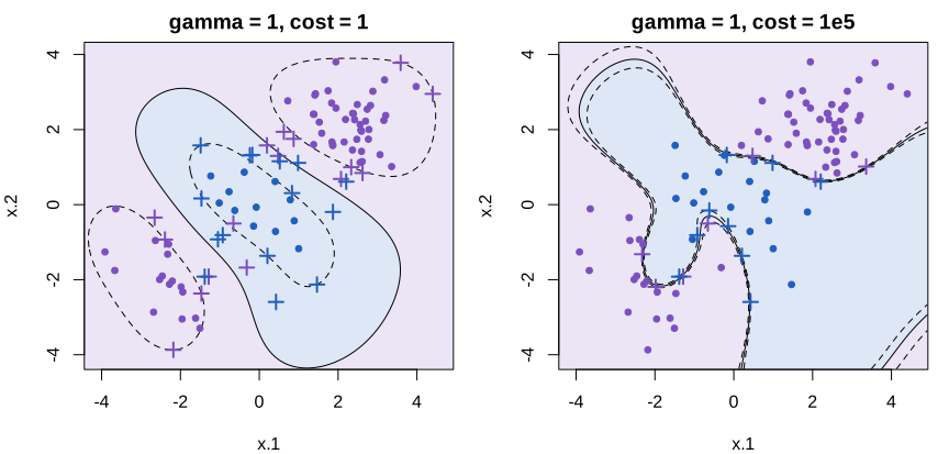
lab-r-radial.svg.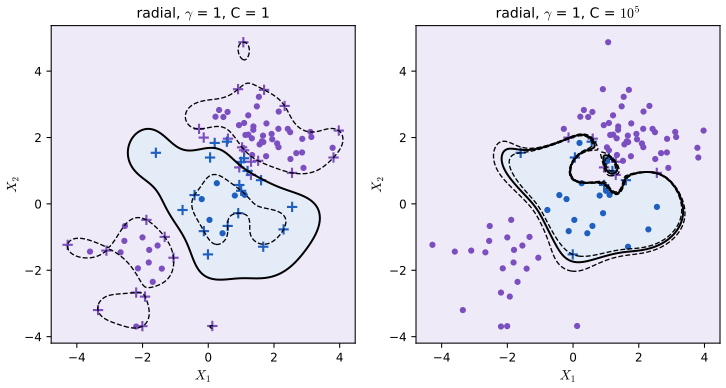
lab-py-radial.svg.A huge cost removes the training errors (6 to 0 in Python) by wrapping the boundary around individual points, a typical overfit. Cross-validation over cost and \(\gamma\):
R
set.seed(1)
tune.out <- tune(svm, y ~ ., data = dat[train, ], kernel = "radial",
                 ranges = list(cost = c(0.1, 1, 10, 100, 1000), gamma = c(0.5, 1, 2, 3, 4)))
summary(tune.out)
tab <- table(true = dat[-train, "y"], pred = predict(tune.out$best.model, newdata = dat[-train, ]))
print(tab)
Python
kfold = skm.KFold(5, random_state=0, shuffle=True)
grid = skm.GridSearchCV(svm_rbf, {"C": [0.1, 1, 10, 100, 1000], "gamma": [0.5, 1, 2, 3, 4]},
                        refit=True, cv=kfold, scoring="accuracy").fit(X_train, y_train)
print("best:", grid.best_params_)
print(pd.DataFrame(grid.cv_results_["mean_test_score"].reshape(5, 5),
                   index=pd.Index([0.1, 1, 10, 100, 1000], name="C"), columns=pd.Index([0.5, 1, 2, 3, 4], name="gamma")))
best_svm = grid.best_estimator_
print(confusion_table(best_svm.predict(X_test), y_test))
- best parameters:
cost gamma
1 0.5
- best performance: 0.07
pred
true 1 2
1 67 10
2 2 21best: {'C': 1, 'gamma': 0.5}
gamma 0.5 1.0 2.0 3.0 4.0
C
0.1 0.76 0.75 0.75 0.75 0.75
1.0 0.91 0.91 0.87 0.86 0.85
10.0 0.88 0.88 0.88 0.86 0.84
100.0 0.89 0.89 0.87 0.85 0.85
1000.0 0.91 0.88 0.86 0.85 0.85
Truth 1 2
Predicted
1 69 6
2 6 19Both choose cost 1 and \(\gamma=0.5\) and misclassify 12% of the test half: 12 of 100 in each language, from different data. The Python edition prints {'C': 100, 'gamma': 1} here; see the notes on the book.
9.6.3 ROC Curves
An SVM's decision values \(\hat f(x)\) are scores; thresholding them at values other than 0 trades the two kinds of error, and the ROC curve shows all thresholds at once. R's predict(..., decision.values = TRUE) and Python's decision_function return them.
R
rocplot <- function(pred, truth, ...) {
  predob <- prediction(pred, truth)
  perf <- performance(predob, "tpr", "fpr")
  plot(perf, ...)
}
auc <- function(pred, truth) performance(prediction(pred, truth), "auc")@y.values[[1]]
svmfit.opt <- svm(y ~ ., data = dat[train, ], kernel = "radial", gamma = 2, cost = 1, decision.values = TRUE)
svmfit.flex <- svm(y ~ ., data = dat[train, ], kernel = "radial", gamma = 50, cost = 1, decision.values = TRUE)
dv <- function(fit, newdata) attributes(predict(fit, newdata, decision.values = TRUE))$decision.values
rocplot(-dv(svmfit.opt, dat[train, ]), dat[train, "y"], main = "Training Data")
rocplot(-dv(svmfit.flex, dat[train, ]), dat[train, "y"], add = TRUE, col = "red")
rocplot(-dv(svmfit.opt, dat[-train, ]), dat[-train, "y"], main = "Test Data")
rocplot(-dv(svmfit.flex, dat[-train, ]), dat[-train, "y"], add = TRUE, col = "red")
aucs <- c(auc(-dv(svmfit.opt, dat[train, ]), dat[train, "y"]), auc(-dv(svmfit.opt, dat[-train, ]), dat[-train, "y"]),
          auc(-dv(svmfit.flex, dat[train, ]), dat[train, "y"]), auc(-dv(svmfit.flex, dat[-train, ]), dat[-train, "y"]))
cat("AUC train/test, gamma 2:", aucs[1:2], " gamma 50:", aucs[3:4], "\n")
Python
# ROC curves from the decision values f(x): positive values predict class 2
svm_flex = SVC(kernel="rbf", gamma=50, C=1).fit(X_train, y_train)
fig, ax = plt.subplots(1, 2, figsize=(9, 4.3))
aucs = []
for k, (Xs, ys, name) in enumerate([(X_train, y_train, "Training data"), (X_test, y_test, "Test data")]):
    for model, colour, lab in [(best_svm, "k", r"$\gamma$ = %g" % best_svm.gamma), (svm_flex, "r", r"$\gamma$ = 50")]:
        score = model.decision_function(Xs)
        fpr, tpr, _ = roc_curve(ys == 2, score)
        auc = roc_auc_score(ys == 2, score)
        aucs.append(auc)
        ax[k].plot(fpr, tpr, colour, label="%s (AUC %.3f)" % (lab, auc))
    ax[k].plot([0, 1], [0, 1], ":", color="0.6")
    ax[k].set(xlabel="False positive rate", ylabel="True positive rate", title=name)
    ax[k].legend(loc="lower right")
common.savefig(fig, 9, "lab-py-roc", formats=("svg",))
print("AUC train (best, gamma 50), test (best, gamma 50):", np.round(aucs, 4))
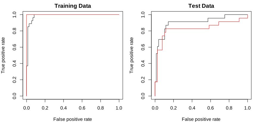
AUC train/test, gamma 2: 0.984779 0.907397 gamma 50: 1 0.828346
AUC train (best, gamma 50), test (best, gamma 50): [0.9925 1. 0.8971 0.808 ]
lab-r-roc.svg.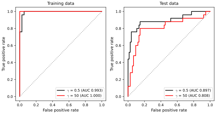
lab-py-roc.svg.In both languages \(\gamma=50\) is perfect on the training half (AUC 1) and the worst on the test half (0.83 and 0.81): flexibility that buys a perfect training ROC curve costs accuracy on new data, the lesson of Figures 9.10 and 9.11. The R lab compares \(\gamma=2\), which it calls svmfit.opt although tune() chose 0.5; the Python lab compares the tuned \(\gamma=0.5\).
9.6.4 SVM with Multiple Classes
R
set.seed(1)
x <- rbind(x, matrix(rnorm(50 * 2), ncol = 2))
y <- c(y, rep(0, 50))
x[y == 0, 2] <- x[y == 0, 2] + 2
dat <- data.frame(x = x, y = as.factor(y))
svmfit <- svm(y ~ ., data = dat, kernel = "radial", cost = 10, gamma = 1)
cat("three classes: support vectors per class", svmfit$nSV, " training errors", sum(svmfit$fitted != dat$y), "\n")
Python
rng = np.random.default_rng(123)
X = np.vstack([X, rng.standard_normal((50, 2))])
y = np.hstack([y, [0] * 50])
X[y == 0, 1] += 2
svm_rbf_3 = SVC(kernel="rbf", C=10, gamma=1, decision_function_shape="ovo").fit(X, y)
print("three classes: support vectors per class", svm_rbf_3.n_support_,
      " training error %.3f" % np.mean(svm_rbf_3.predict(X) != y))
# one-versus-one by hand: the three pairwise votes give the same labels as predict()
D = svm_rbf_3.decision_function(X)              # columns: (0 vs 1), (0 vs 2), (1 vs 2); positive = first class
votes = np.zeros((len(y), 3))
for col, (a, b) in enumerate([(0, 1), (0, 2), (1, 2)]):
    votes[:, a] += D[:, col] > 0
    votes[:, b] += D[:, col] <= 0
print("hand-counted votes reproduce predict():", np.array_equal(svm_rbf_3.classes_[votes.argmax(1)], svm_rbf_3.predict(X)))
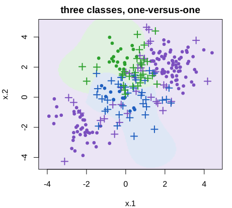
three classes: support vectors per class 38 37 30 training errors 38
three classes: support vectors per class [40 69 31]  training error 0.160
hand-counted votes reproduce predict(): True
lab-r-three.svg.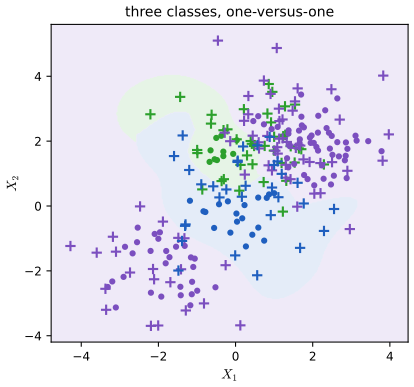
lab-py-three.svg.The third class, shifted up by 2, overlaps both others heavily, so 15% (R) and 16% (Python) of the training points are misclassified. In Python the three pairwise decision values, counted as votes, give exactly the predictions of predict() (Algorithm 9.2). Both functions also do support vector regression when the response is numerical.
9.6.5 Application to Gene Expression Data
The Khan data contain the expression of 2308 genes for 63 training and 20 test tissue samples of four types of small round blue cell tumours. With \(p\gg n\) a linear kernel is enough: there are many hyperplanes that separate the training data, and more flexibility would only add variance. In Python the data come from the R package ISLR2, written once to cache/ by the R script.
R
dat <- data.frame(x = Khan$xtrain, y = as.factor(Khan$ytrain))
out <- svm(y ~ ., data = dat, kernel = "linear", cost = 10)
summary(out)
table(out$fitted, dat$y)
dat.te <- data.frame(x = Khan$xtest, y = as.factor(Khan$ytest))
pred.te <- predict(out, newdata = dat.te)
table(pred.te, dat.te$y)
raw <- svm(Khan$xtrain, as.factor(Khan$ytrain), kernel = "linear", cost = 10, scale = FALSE)
cat("unscaled genes (as in the Python lab): support vectors", raw$nSV, " test errors",
    sum(predict(raw, Khan$xtest) != Khan$ytest), "\n")
# one-versus-all (Section 9.4.2), which svm() does not offer: four "class k against the rest" fits
ova <- sapply(1:4, function(k) {
  f <- svm(Khan$xtrain, factor(Khan$ytrain == k), kernel = "linear", cost = 10, scale = FALSE)
  dv <- attr(predict(f, Khan$xtest, decision.values = TRUE), "decision.values")
  if (startsWith(colnames(dv), "TRUE")) dv else -dv        # orient so that f > 0 means "class k"
})
pred.ova <- max.col(ova)
Python
khan_linear = SVC(kernel="linear", C=10).fit(khan["xtrain"], khan["ytrain"])
print(confusion_table(khan_linear.predict(khan["xtrain"]), khan["ytrain"]))
print(confusion_table(khan_linear.predict(khan["xtest"]), khan["ytest"]))
print("support vectors per class:", khan_linear.n_support_)
# with every gene standardised first, as e1071::svm() does by default in the R lab
sc = e1071_scale(khan["xtrain"])
khan_scaled = SVC(kernel="linear", C=10).fit(sc(khan["xtrain"]), khan["ytrain"])
print("standardised genes: support vectors", khan_scaled.n_support_, " test errors",
      np.sum(khan_scaled.predict(sc(khan["xtest"])) != khan["ytest"]))
# one-versus-all (Section 9.4.2): SVC itself always fits the K(K - 1)/2 pairwise classifiers, even with
# decision_function_shape="ovr"; OneVsRestClassifier fits K "class k against the rest" classifiers
ova = OneVsRestClassifier(SVC(kernel="linear", C=10)).fit(khan["xtrain"], khan["ytrain"])
print("one-versus-all: test errors", np.sum(ova.predict(khan["xtest"]) != khan["ytest"]))
Number of Support Vectors: 58
( 20 20 11 7 )
pred.te 1 2 3 4
1 3 0 0 0
2 0 6 2 0
3 0 0 4 0
4 0 0 0 5
unscaled genes (as in the Python lab): support vectors 18 20 9 7 test errors 2
one-versus-all: test errors 0Truth 1 2 3 4 Predicted 1 3 0 0 0 2 0 6 2 0 3 0 0 4 0 4 0 0 0 5 support vectors per class: [ 7 18 9 20] standardised genes: support vectors [ 7 20 11 20] test errors 2 one-versus-all: test errors 0
No training errors (not shown) and two test errors, both type-3 tumours called type 2, in both editions: R with standardised genes (the default) and Python without. Each language also fits the other edition's version, with the same result. (e1071 lists the support-vector counts in the order in which the classes first appear in the data, scikit-learn in sorted order: 20 20 11 7 and 7 20 11 20 are the same counts.) The one-versus-all fits of Section 9.4.2, four "class \(k\) against the rest" SVMs, classify all 20 test samples correctly here, in both languages; with 20 test samples that is suggestive, not conclusive.
Notes on the book
The Python lab's Out[24] does not match its own text
After the grid search over \(C\in\{0.1,\dots,1000\}\) and \(\gamma\in\{0.5,\dots,4\}\) (In[24], p. 391 of the 2023 edition) the book prints {'C': 100, 'gamma': 1}, but the next sentence says the best choice is "C=1 and gamma=0.5", and the test table that follows (69, 6, 6, 19) is the one of \(C=1,\gamma=0.5\). Rerunning the cell gives {'C': 1, 'gamma': 0.5}: the five-fold accuracy of \((C,\gamma)=(100,1)\) is 0.89, below the 0.91 of \((1,0.5)\), \((1,1)\) and \((1000,0.5)\). The printed output is stale.
The Python lab: decision_function_shape='ovr' is not one-versus-rest fitting
Section 9.6.4 of the 2023 edition says that SVC() "will perform multi-class classification using either the one-versus-one approach (when decision_function_shape=='ovo') or one-versus-rest (when decision_function_shape=='ovr')". In fact SVC always trains the \(\binom K2\) one-versus-one classifiers; the option only changes the shape of the decision values it returns (an \(n\times K\) table built from the pairwise votes), and the predictions are the same. With the Khan data the fitted support vectors and coefficients are identical under both settings. A one-versus-all fit as in Section 9.4.2 needs OneVsRestClassifier; it gives 0 test errors on the Khan data, against 2 for one-versus-one (Section 9.6.5 here).
The linear kernel and "Pearson correlation"
Section 9.3.2 (p. 382, both editions) says that the linear kernel "essentially quantifies the similarity of a pair of observations using Pearson (standard) correlation". The inner product \(\sum_jx_{ij}x_{i'j}\) is a correlation only after each observation's vector of \(p\) values has been centred (across its features) and scaled to length 1; otherwise it grows with the lengths of the two vectors. Inner product and correlation give quite different similarities for raw data, for example two expression profiles that differ by a constant factor are perfectly correlated but have very different inner products with a third.
Small budgets are infeasible for non-separable data
Section 9.2.2 treats the budget \(C\) as a tuning parameter that can be taken from 0 upwards. For data that no hyperplane separates, (9.12)–(9.15) has no solution with \(M>0\) when \(C\) is below the smallest total hinge loss \(\min\sum_i\max[0,1-y_if(x_i)]\) (Result 9.4); for the R lab's 20 overlapping points that is \(C<4.99\). In the cost form used by the software this shows up as a fit that stops changing beyond some cost: on those 20 points every cost from about 10 up gives the same hyperplane, which is why tune() reports identical errors for costs 1 to 100 (cost 1 is already very close to it).
The R lab scales the features without saying so
The R lab passes scale = FALSE in its first fits and explains the argument, but the later calls (the separable data with cost = 1e5, all radial fits, the three-class fit and the Khan data) use the default scale = TRUE. The kernels and \(\gamma\) values discussed in Sections 9.6.2–9.6.4 therefore apply to standardised features, while the Python lab's identically named fits use the raw ones. The numbers printed in each edition are right for its own code.
Exercises
Conceptual exercises 1–3 and applied exercises 4–8, in the book's numbering (the two editions have the same exercises; the Python edition generates the data of Exercise 5 with default_rng(5)). The applied solutions are the last sections of ch09_lab.R and ch09_lab.py. So that both languages see the same data, simulated inputs come from the deterministic sequence \(u_i=\mathrm{frac}(i\sqrt{p_k})\) (\(p_k\) the \(k\)-th prime) instead of a random number generator, normal variables are \(\Phi^{-1}(u_i)\), cross-validation folds are fixed by row number (row \(i\) in fold \(i\bmod10\)), and the OJ training set is a fixed permutation. All numbers below are identical in R and Python.
R
qrand <- function(n, k, start = 1) {
  a <- sqrt(c(2, 3, 5, 7, 11, 13, 17, 19, 23, 29, 31, 37)[k]) %% 1
  (seq(start, length.out = n) * a) %% 1
}
cv_error <- function(x, y, ..., K = 10) {               # K folds, row i in fold (i - 1) mod K
  fold <- (seq_along(y) - 1) %% K
  wrong <- 0
  for (k in 0:(K - 1)) {
    fit <- svm(x[fold != k, , drop = FALSE], y[fold != k], scale = FALSE, ...)
    wrong <- wrong + sum(predict(fit, x[fold == k, , drop = FALSE]) != y[fold == k])
  }
  wrong / length(y)
}
err <- function(fit, x, y) mean(predict(fit, x) != y)
Python
def qrand(n, k, start=1):
    """n numbers in [0, 1) from stream k: frac(i * sqrt(p_k)), i = start, ..., start + n - 1, p_k the
    k-th prime (a Weyl sequence). The exercises use it so that R and Python get identical data."""
    a = np.sqrt([2, 3, 5, 7, 11, 13, 17, 19, 23, 29, 31, 37][k - 1]) % 1
    return (np.arange(start, start + n) * a) % 1

def cv_error(make_model, X, y, K=10):
    """K-fold cross-validated misclassification rate, row i in fold (i mod K) (as in the R lab)."""
    fold = np.arange(len(y)) % K
    wrong = 0
    for k in range(K):
        m = make_model().fit(X[fold != k], y[fold != k])
        wrong += np.sum(m.predict(X[fold == k]) != y[fold == k])
    return wrong / len(y)
Exercise 9.1. In the plane, sketch the hyperplane \(1+3X_1-X_2=0\) and mark where \(1+3X_1-X_2>0\) and \(<0\). On the same plot do the same for \(-2+X_1+2X_2=0\).
Solution
The first hyperplane is the line \(X_2=1+3X_1\) (slope 3, through \((0,1)\) and \((-\tfrac13,0)\)). Since the coefficient of \(X_2\) is \(-1\), \(1+3X_1-X_2>0\) means \(X_2<1+3X_1\): the region below (to the right of) the line; above it the expression is negative. Its normal \((3,-1)\) points into the positive side (Result 9.1). The second is the line \(X_2=1-X_1/2\) (through \((0,1)\) and \((2,0)\)); \(-2+X_1+2X_2>0\) means \(X_2>1-X_1/2\), the region above it, with normal \((1,2)\). The two lines cross at \((0,1)\) and divide the plane into four regions with the four sign combinations.
Exercise 9.2. (a) Sketch the curve \((1+X_1)^2+(2-X_2)^2=4\). (b) Mark where the left side is \(>4\) and where it is \(\le4\). (c) A classifier predicts blue if \((1+X_1)^2+(2-X_2)^2>4\) and red otherwise: classify \((0,0)\), \((-1,1)\), \((2,2)\), \((3,8)\). (d) Show the boundary is linear in \(X_1,X_1^2,X_2,X_2^2\).
Solution
(a) A circle with centre \((-1,2)\) and radius 2. (b) \(>4\): outside the circle; \(\le4\): the closed disc. (c) \((0,0)\): \(1+4=5>4\), blue. \((-1,1)\): \(0+1=1\), red. \((2,2)\): \(9+0=9\), blue. \((3,8)\): \(16+36=52\), blue. (d) Expanding, \((1+X_1)^2+(2-X_2)^2-4=1+2X_1+X_1^2-4X_2+X_2^2\), so the classifier is "blue if \(1+2X_1+X_1^2-4X_2+X_2^2>0\)": a hyperplane in the four features \(X_1,X_1^2,X_2,X_2^2\) with \(\beta_0=1\), \(\bb=(2,1,-4,1)\). This is the enlarged feature space of (9.16).
Exercise 9.3. Seven points: red \((3,4),(2,2),(4,4),(1,4)\) and blue \((2,1),(4,3),(4,1)\). (a) Sketch them. (b) Sketch and give the equation of the optimal separating hyperplane. (c) State the rule "red if \(\beta_0+\beta_1X_1+\beta_2X_2>0\)". (d) Mark the margin. (e) Name the support vectors. (f) Why does a small move of observation 7 not change the hyperplane? (g) Give a separating hyperplane that is not optimal. (h) Add a point that makes the classes non-separable.
Solution
(a), (b) The red points lie on or above the line \(X_2=X_1\), the blue ones below it. The closest opposite pairs are \((2,2)\) red with \((2,1)\) blue and \((4,4)\) red with \((4,3)\) blue, each pair one unit apart vertically. The maximal margin hyperplane runs halfway between the parallel lines \(X_2=X_1\) (through the red pair) and \(X_2=X_1-1\) (through the blue pair): \(X_2=X_1-0.5\), that is \(0.5-X_1+X_2=0\).
(c) Red if \(0.5-X_1+X_2>0\), blue otherwise: \(\beta_0=0.5\), \(\beta_1=-1\), \(\beta_2=1\). (d) The margin lines are \(X_2=X_1\) and \(X_2=X_1-1\); the margin is the distance from \((2,2)\) to the hyperplane, \(|0.5-2+2|/\sqrt2=1/(2\sqrt2)=0.354\). (e) The support vectors are observations 2 \((2,2)\), 3 \((4,4)\), 5 \((2,1)\) and 6 \((4,3)\). (f) Observation 7 \((4,1)\) is at distance \(|0.5-4+1|/\sqrt2=1.77\), far beyond the margin; its multiplier is 0 (Filling the gap 9.3), so a small move that keeps it outside the margin leaves the solution unchanged. (g) For example \(0.2-X_1+X_2=0\): every red point gives a positive value (at least 0.2) and every blue one a negative value (at most \(-0.8\)), but the margin is only \(0.2/\sqrt2=0.14\). (h) A blue point at \((2,3)\) lies inside the triangle of the red points \((1,4),(2,2),(3,4)\), so no line can separate it from them. Confirmed numerically by solving the quadratic programme of Result 9.2.
Exercise 9.4. Simulate two classes with 100 observations and two features separated by a visible non-linear boundary. Show that an SVM with a polynomial kernel (degree above 1) or a radial kernel beats the support vector classifier on the training data. Which is best on test data?
Solution
Points uniform on \([-2,2]^2\), class \(+1\) when \(X_2-(X_1^2-1.5)+0.3Z>0\) (a parabola, blurred by noise \(Z\sim\N(0,1)\)); 100 training and 100 test points; cost 1, no scaling; the polynomial kernel is \((1+\langle x,z\rangle)^2\) as in (9.22).
R
# Exercise 4
n <- 200
x1 <- 4 * qrand(n, 1) - 2; x2 <- 4 * qrand(n, 2) - 2; z <- qnorm(qrand(n, 3))
y4 <- as.factor(ifelse(x2 - (x1^2 - 1.5) + 0.3 * z > 0, 1, -1))
X4 <- cbind(x1, x2); tr <- seq_len(n) <= 100
f_lin <- svm(X4[tr, ], y4[tr], kernel = "linear", cost = 1, scale = FALSE)
f_pol <- svm(X4[tr, ], y4[tr], kernel = "polynomial", degree = 2, gamma = 1, coef0 = 1, cost = 1, scale = FALSE)
f_rbf <- svm(X4[tr, ], y4[tr], kernel = "radial", gamma = 1, cost = 1, scale = FALSE)
ex4 <- sapply(list(f_lin, f_pol, f_rbf), function(f) c(err(f, X4[tr, ], y4[tr]), err(f, X4[!tr, ], y4[!tr])))
print(round(ex4, 2))                                    # columns: linear, polynomial, radial; rows: training, test
Python
# Exercise 4: a curved boundary; 100 training and 100 test points
n = 200
x1, x2, z = 4 * qrand(n, 1) - 2, 4 * qrand(n, 2) - 2, norm.ppf(qrand(n, 3))
y = np.where(x2 - (x1 ** 2 - 1.5) + 0.3 * z > 0, 1, -1)
X, tr = np.column_stack([x1, x2]), np.arange(n) < 100
ex4 = []
for name, model in [("linear", SVC(kernel="linear", C=1)),
                    ("polynomial, d = 2", SVC(kernel="poly", degree=2, gamma=1, coef0=1, C=1)),
                    ("radial, gamma = 1", SVC(kernel="rbf", gamma=1, C=1))]:
    model.fit(X[tr], y[tr])
    e = [np.mean(model.predict(X[tr]) != y[tr]), np.mean(model.predict(X[~tr]) != y[~tr])]
    print("Exercise 4, %-18s training error %.2f, test error %.2f" % (name, *e))
    ex4 += e
training error test error linear 0.25 0.28 polynomial, d = 2 0.06 0.04 radial, gamma = 1 0.05 0.07
Both kernels cut the training error from 0.25 to about 0.05; on the test data the quadratic kernel, which has exactly the shape of the true boundary, is best (0.04), the radial kernel a little worse (0.07), and the linear classifier far behind (0.28).
Exercise 9.5. With \(n=500\), \(p=2\) and a quadratic boundary (\(X_1,X_2\) uniform on \([-0.5,0.5]\), class 1 when \(X_1^2-X_2^2>0\)), compare logistic regression on \(X_1,X_2\), logistic regression with non-linear functions of them, the support vector classifier, and an SVM with a non-linear kernel, by their predicted labels on the training data.
Solution
A little noise, \(0.02Z\), is added to \(X_1^2-X_2^2\) so that the classes overlap slightly and the logistic fit with quadratic terms has a finite maximum (without it the classes are separated by the quadratic model and the coefficients diverge). Radial kernel with \(\gamma=10\), cost 10.
R
# Exercise 5
n <- 500
x1 <- qrand(n, 4) - 0.5; x2 <- qrand(n, 5) - 0.5; z <- qnorm(qrand(n, 6))
y5 <- as.integer(x1^2 - x2^2 + 0.02 * z > 0)
lin <- glm(y5 ~ x1 + x2, family = binomial)
quad <- glm(y5 ~ x1 + x2 + I(x1^2) + I(x2^2) + I(x1 * x2), family = binomial)
svc5 <- svm(cbind(x1, x2), as.factor(y5), kernel = "linear", cost = 1, scale = FALSE)
rbf5 <- svm(cbind(x1, x2), as.factor(y5), kernel = "radial", gamma = 10, cost = 10, scale = FALSE)
ex5 <- c(mean((fitted(lin) > 0.5) != y5), mean((fitted(quad) > 0.5) != y5),
         err(svc5, cbind(x1, x2), y5), err(rbf5, cbind(x1, x2), y5))
print(round(ex5, 3)); print(round(coef(quad), 3))
Python
# Exercise 5: logistic regression with non-linear features against an SVM
n = 500
x1, x2, z = qrand(n, 4) - 0.5, qrand(n, 5) - 0.5, norm.ppf(qrand(n, 6))
y = (x1 ** 2 - x2 ** 2 + 0.02 * z > 0).astype(int)
X = np.column_stack([x1, x2])
lin = sm.GLM(y, sm.add_constant(X), family=sm.families.Binomial()).fit()
Q = np.column_stack([x1, x2, x1 ** 2, x2 ** 2, x1 * x2])
quad = sm.GLM(y, sm.add_constant(Q), family=sm.families.Binomial()).fit()
svc = SVC(kernel="linear", C=1).fit(X, y)
rbf = SVC(kernel="rbf", gamma=10, C=10).fit(X, y)
e5 = [np.mean((lin.fittedvalues > 0.5) != y), np.mean((quad.fittedvalues > 0.5) != y),
      np.mean(svc.predict(X) != y), np.mean(rbf.predict(X) != y)]
print("Exercise 5: training errors, logistic linear %.3f, logistic quadratic %.3f, SVC %.3f, radial SVM %.3f" % tuple(e5))
print("  quadratic logistic coefficients:", quad.params.round(3))
training error: logistic (X1, X2) 0.468 logistic (quadratic) 0.080 SVC 0.468 radial SVM 0.086 quadratic logistic coefficients: -0.152 0.058 0.361 83.089 -81.876 -0.402
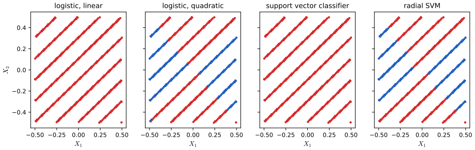
Exercise 5 (Python): predicted classes of the four methods. Both linear methods give up: the classes occupy opposite quadrant pairs, no line does better than predicting the majority class everywhere, and the training error is the minority proportion 0.468. The logistic model with \(X_1^2\), \(X_2^2\) and \(X_1X_2\) recovers the boundary almost exactly (coefficients near \(+83\) and \(-82\) on the squares, so \(\hat f\approx83(X_1^2-X_2^2)\)), with error 0.080, close to the noise level; the radial SVM does as well (0.086) without being told the form of the boundary. Non-linear features make logistic regression as flexible as a kernel SVM when the right features are known.
Exercise 9.6. Investigate the claim at the end of Section 9.6.1: for barely separable data, a small cost that misclassifies a few training points may do better on test data than a huge cost that misclassifies none. Report training errors, cross-validation errors and test errors over a range of costs.
Solution
Training data: 100 points uniform on \([-2,2]^2\), labelled by the side of the line \(X_2=X_1\), with a gap of 0.3 around it, plus two class-\(+1\) points just below the line at \((1.2,1.05)\) and \((1.5,1.38)\). The data remain separable, but only by a tilted line. Test data: 2000 new points labelled by the true line.
R
# Exercise 6
x1 <- 4 * qrand(200, 7) - 2; x2 <- 4 * qrand(200, 8) - 2
X6 <- cbind(x1, x2)[abs(x2 - x1) > 0.3, ][1:100, ]
X6 <- rbind(X6, c(1.2, 1.05), c(1.5, 1.38))
y6 <- as.factor(c(ifelse(X6[1:100, 2] > X6[1:100, 1], 1, -1), 1, 1))
xt1 <- 4 * qrand(2000, 7, start = 1001) - 2; xt2 <- 4 * qrand(2000, 8, start = 1001) - 2
Xt6 <- cbind(xt1, xt2); yt6 <- ifelse(xt2 > xt1, 1, -1)
ex6 <- t(sapply(c(0.01, 0.1, 1, 10, 100, 1000, 10000), function(cost) {
  f <- svm(X6, y6, kernel = "linear", cost = cost, scale = FALSE)
  c(cost = cost, train_errors = sum(predict(f, X6) != y6), cv = cv_error(X6, y6, kernel = "linear", cost = cost),
    test = err(f, Xt6, yt6))
}))
print(ex6)
Python
# Exercise 6: barely separable training data; two class-1 points sit just below the true line
x1, x2 = 4 * qrand(200, 7) - 2, 4 * qrand(200, 8) - 2
gap = np.abs(x2 - x1) > 0.3
X = np.column_stack([x1, x2])[gap][:100]
X = np.vstack([X, [[1.2, 1.05], [1.5, 1.38]]])
y = np.r_[np.where(X[:100, 1] > X[:100, 0], 1, -1), 1, 1]
xt1, xt2 = 4 * qrand(2000, 7, start=1001) - 2, 4 * qrand(2000, 8, start=1001) - 2
Xt, yt = np.column_stack([xt1, xt2]), np.where(xt2 > xt1, 1, -1)
costs = [0.01, 0.1, 1, 10, 100, 1000, 10000]
rows = []
for c in costs:
    m = SVC(kernel="linear", C=c).fit(X, y)
    rows.append([c, np.sum(m.predict(X) != y), cv_error(lambda: SVC(kernel="linear", C=c), X, y),
                 np.mean(m.predict(Xt) != yt)])
t6 = pd.DataFrame(rows, columns=["cost", "training errors", "CV error", "test error"])
print("Exercise 6\n", t6.to_string(index=False))
cost training errors CV error test error 0.01 0 0.049020 0.0425 0.10 0 0.019608 0.0230 1.00 2 0.019608 0.0150 10.00 0 0.019608 0.0220 100.00 0 0.000000 0.0535 1000.00 0 0.000000 0.0535 10000.00 0 0.000000 0.0535Costs of 100 and more give the hard-margin solution: no training errors, and it tilts to accommodate the two awkward points, with test error 0.054. Cost 1 gives up on those two points (2 training errors) and has the lowest test error, 0.015, more than three times smaller. The claim holds. Cross-validation does not find it here, however: its error is smallest (0) for the large costs. When one of the two awkward points is left out, the other one still tilts the hard-margin line enough to classify it correctly, so no fold ever sees the price of the tilt. With so few influential points cross-validation is noisy, and the training error is a poor guide in both directions.
Exercise 9.7. Predict whether a car's gas mileage in the Auto data is above the median: (a) create the binary response; (b) fit support vector classifiers for several costs and report cross-validation errors; (c) repeat with radial and polynomial kernels for several \(\gamma\), degrees and costs; (d) make plots.
Solution
The seven predictors other than
mpgandname(cylinders, displacement, horsepower, weight, acceleration, year, origin), standardised; ten folds by row number. Leavingmpgin would give a trivial perfect classifier.R
# Exercise 7
Auto7 <- na.omit(Auto)
y7 <- as.factor(as.integer(Auto7$mpg > median(Auto7$mpg)))
X7 <- scale(as.matrix(Auto7[, c("cylinders", "displacement", "horsepower", "weight", "acceleration", "year", "origin")]))
cv_lin <- sapply(c(0.01, 0.1, 1, 10, 100), function(cost) cv_error(X7, y7, kernel = "linear", cost = cost))
cv_rbf <- t(sapply(c(0.01, 0.1, 1), function(g) sapply(c(0.1, 1, 10, 100), function(cost)
  cv_error(X7, y7, kernel = "radial", gamma = g, cost = cost))))
cv_pol <- t(sapply(2:3, function(d) sapply(c(0.01, 0.1, 1, 10), function(cost)
  cv_error(X7, y7, kernel = "polynomial", degree = d, gamma = 1, coef0 = 1, cost = cost))))
print(round(cv_lin, 4)); print(round(cv_rbf, 4)); print(round(cv_pol, 4))
Python
# Exercise 7: high or low mileage in the Auto data, ten folds by row number
Auto = common.isl_data("Auto", na_values="?").dropna().reset_index(drop=True)
y = np.where(Auto["mpg"] > Auto["mpg"].median(), 1, 0)
X = Auto[["cylinders", "displacement", "horsepower", "weight", "acceleration", "year", "origin"]].to_numpy(float)
X = e1071_scale(X)(X)
cv_lin = [cv_error(lambda: SVC(kernel="linear", C=c), X, y) for c in (0.01, 0.1, 1, 10, 100)]
cv_rbf = [[cv_error(lambda: SVC(kernel="rbf", gamma=g, C=c), X, y) for c in (0.1, 1, 10, 100)] for g in (0.01, 0.1, 1)]
cv_pol = [[cv_error(lambda: SVC(kernel="poly", degree=d, gamma=1, coef0=1, C=c), X, y) for c in (0.01, 0.1, 1, 10)] for d in (2, 3)]
linear, cost 0.01 0.1 1 10 100: 0.0918 0.1020 0.1097 0.0944 0.0918 radial gamma 0.01, cost 0.1 1 10 100: 0.1148 0.0918 0.0918 0.0867 radial gamma 0.1: 0.0918 0.0918 0.0791 0.0893 radial gamma 1: 0.0867 0.0714 0.0816 0.0918 polynomial degree 2, cost 0.01 0.1 1 10: 0.0969 0.0944 0.0995 0.1148 polynomial degree 3: 0.0791 0.0893 0.0995 0.1327
A linear boundary already misclassifies only about 9% to 11% of the cars, with little dependence on the cost. The radial kernel does best, 7.1% at \(\gamma=1\), cost 1; very flexible fits (radial with large cost, polynomial of degree 3 with cost 10) get worse again (13.3%). With 392 cars, differences of one or two percentage points are four to eight cars and should not be over-read. For (d), pairs of predictors can be plotted with the fitted classes, as in the lab's
plot_fit/plot_svmapplied to two columns at a time.Exercise 9.8. OJ data (1070 purchases of Citrus Hill or Minute Maid orange juice): (a) a training set of 800 observations and a test set of the rest; (b) a support vector classifier with cost 0.01 for
Purchaseon all other variables: how many support vectors? (c) training and test error rates; (d) choose the cost in \([0.01,10]\) by cross-validation; (e) errors at that cost; (f) the same with a radial kernel (default \(\gamma\)); (g) with a polynomial kernel of degree 2; (h) which is best?Solution
The training set is rows \(377i\bmod1070\), \(i=0,\dots,799\) (a fixed permutation); the 17 predictors (Store7 as a 0/1 column) are standardised with the training means and standard deviations, as
svm()does by default. "Default \(\gamma\)" issvm()'s \(1/p=1/17\) (scikit-learn's default differs, so it is given explicitly), and the degree-2 polynomial kernel issvm()'s \((\gamma\langle x,z\rangle)^2\). Costs \(0.01,0.0316,0.1,\dots,10\).R
# Exercise 8
X8 <- model.matrix(Purchase ~ ., data = OJ)[, -1]
perm <- (0:(nrow(OJ) - 1) * 377) %% nrow(OJ)
tr <- seq_len(nrow(OJ)) %in% (perm[1:800] + 1)
Xtr <- scale(X8[tr, ])
Xte <- scale(X8[!tr, ], center = attr(Xtr, "scaled:center"), scale = attr(Xtr, "scaled:scale"))
ytr <- OJ$Purchase[tr]; yte <- OJ$Purchase[!tr]
grid8 <- c(0.01, 0.0316, 0.1, 0.316, 1, 3.16, 10)
p8 <- ncol(X8)
kernels <- list(linear = list(kernel = "linear"), radial = list(kernel = "radial", gamma = 1 / p8),
                polynomial = list(kernel = "polynomial", degree = 2, gamma = 1 / p8, coef0 = 0))
ex8 <- c()
for (nm in names(kernels)) {
  fit <- function(cost) do.call(svm, c(list(x = Xtr, y = ytr, cost = cost, scale = FALSE), kernels[[nm]]))
  f0 <- fit(0.01)
  cv <- sapply(grid8, function(cost) do.call(cv_error, c(list(x = Xtr, y = ytr, cost = cost), kernels[[nm]])))
  cbest <- grid8[which.min(cv)]
  fb <- fit(cbest)
  row <- c(sum(f0$nSV), err(f0, Xtr, ytr), err(f0, Xte, yte), cbest, err(fb, Xtr, ytr), err(fb, Xte, yte))
  cat(sprintf("Exercise 8, %-10s cost 0.01: %d SVs, train %.4f test %.4f; best cost %g: train %.4f test %.4f\n",
              nm, row[1], row[2], row[3], row[4], row[5], row[6]))
  ex8 <- c(ex8, row)
}
Python
# Exercise 8: the OJ data, 800 training rows chosen by a fixed permutation
OJ = common.isl_data("OJ")
y = OJ["Purchase"].to_numpy()
X = OJ.drop(columns="Purchase").assign(Store7=(OJ["Store7"] == "Yes").astype(float)).to_numpy(float)
perm = (np.arange(len(y)) * 377) % len(y)
tr = np.zeros(len(y), bool)
tr[perm[:800]] = True
sc = e1071_scale(X[tr])
Xtr, Xte, ytr, yte = sc(X[tr]), sc(X[~tr]), y[tr], y[~tr]
p = X.shape[1]
grid = [0.01, 0.0316, 0.1, 0.316, 1, 3.16, 10]
kernels = {"linear": dict(kernel="linear"), "radial": dict(kernel="rbf", gamma=1 / p),
           "polynomial": dict(kernel="poly", degree=2, gamma=1 / p, coef0=0)}
out8 = []
for name, kw in kernels.items():
    m = SVC(C=0.01, **kw).fit(Xtr, ytr)
    e0 = [np.mean(m.predict(Xtr) != ytr), np.mean(m.predict(Xte) != yte)]
    cv = [cv_error(lambda: SVC(C=c, **kw), Xtr, ytr) for c in grid]
    cbest = grid[int(np.argmin(cv))]
    mb = SVC(C=cbest, **kw).fit(Xtr, ytr)
    e1 = [np.mean(mb.predict(Xtr) != ytr), np.mean(mb.predict(Xte) != yte)]
    print("Exercise 8, %-10s cost 0.01: %d support vectors, errors train %.4f test %.4f; best cost %g: train %.4f test %.4f"
          % (name, m.n_support_.sum(), *e0, cbest, *e1))
    out8 += [m.n_support_.sum(), *e0, cbest, *e1]
cost 0.01: SVs train test best cost train test linear 438 0.1638 0.1741 3.16 0.1613 0.1667 radial 621 0.3850 0.4037 1 0.1437 0.1741 polynomial 625 0.3850 0.4037 10 0.2100 0.1926
(b), (c) With cost 0.01 the linear classifier uses 438 of the 800 purchases as support vectors (a very wide margin) and errs on 16.4% of the training and 17.4% of the test purchases; the radial and polynomial kernels at that cost predict Citrus Hill for everyone (error = the Minute Maid share). (d), (e) After tuning: linear 16.7% test error, radial 17.4%, polynomial 19.3%. (h) The linear classifier is best, or at least as good as any; customer loyalty to Citrus Hill (
LoyalCH) and the price difference carry most of the signal, and they act roughly linearly. Test sets of 270 purchases cannot distinguish 16.7% from 17.4%.
Demonstrations for this chapter
Each demonstration runs in the browser on the book's data and links back to these notes. The ▶ Demo boxes above open them already set to the case under discussion.
| Demonstration | What you can see | Sections |
|---|---|---|
| The budget C: from the maximal margin to the soft margin | The support vector classifier in the book's budget form on the R lab's 20 points: the hyperplane and margins, the slack \(\epsilon_i\) of every point, the support vectors, \(M\) and their number against \(C\), and the equivalent cost and \(\lambda\); click to add points. Presets: 1 budget 0, the maximal margin; 2 a small budget; 3 a large budget; 4 overlapping classes, smallest budget; 5 overlapping classes, budget 12. | 9.1.4, 9.2.2, 9.6.1 |
| Radial kernels on the Heart data: training and test ROC curves | Linear and radial SVMs fitted to 207 patients for any \(\gamma\) and cost: the ROC curves and AUC on the training and test patients, the AUC against \(\gamma\), the scores by disease status, and LDA for comparison. Presets: 1 support vector classifier and LDA; 2 \(\gamma=0.001\); 3 \(\gamma=0.01\); 4 \(\gamma=0.1\); 5 \(\gamma=1\). | 9.3.2, 9.3.3, 9.6.3 |
| Hinge loss against logistic loss: who pulls on the boundary | The support vector classifier (9.25) and ridge-penalised logistic regression with the same \(\lambda\) on the Python lab's 50 points: both boundaries, every observation on its loss curve (Figure 9.12), the weight of each observation in each fit, and what happens when the well-classified points move away. Presets: 1 \(\lambda=0.05\); 2 \(\lambda=0.5\); 3 \(\lambda=5\); 4 pushing points away; 5 \(\lambda=2\). | 9.5 |
Related demonstrations in the companion courses: the whole regularisation path of the SVM on the mixture data and maximum margin, soft margin and support vector regression with an SMO solver; and, for ROC curves, the threshold and the ROC curve on the Default data (Chapter 4).
References
- James, G., Witten, D., Hastie, T. and Tibshirani, R. (2021). An Introduction to Statistical Learning with Applications in R, 2nd edition. Springer, New York. Chapter 9, pp. 367–402. www.statlearning.com.
- James, G., Witten, D., Hastie, T., Tibshirani, R. and Taylor, J. (2023). An Introduction to Statistical Learning with Applications in Python. Springer, Cham. Chapter 9.
- Boser, B. E., Guyon, I. M. and Vapnik, V. N. (1992). A training algorithm for optimal margin classifiers. Proceedings of the Fifth Annual Workshop on Computational Learning Theory, 144–152.
- Chang, C.-C. and Lin, C.-J. (2011). LIBSVM: a library for support vector machines. ACM Transactions on Intelligent Systems and Technology, 2(3), 27.
- Cortes, C. and Vapnik, V. (1995). Support-vector networks. Machine Learning, 20, 273–297.
- Fan, R.-E., Chen, P.-H. and Lin, C.-J. (2005). Working set selection using second order information for training support vector machines. Journal of Machine Learning Research, 6, 1889–1918.
- Hastie, T., Tibshirani, R. and Friedman, J. (2009). The Elements of Statistical Learning, 2nd edition. Springer, New York. Sections 4.5 and 12.1–12.3.
- Khan, J., Wei, J. S., Ringnér, M. et al. (2001). Classification and diagnostic prediction of cancers using gene expression profiling and artificial neural networks. Nature Medicine, 7, 673–679.
- Platt, J. (1998). Sequential minimal optimization: a fast algorithm for training support vector machines. Microsoft Research Technical Report MSR-TR-98-14.
- Platt, J. (1999). Probabilistic outputs for support vector machines and comparisons to regularized likelihood methods. In Advances in Large Margin Classifiers, MIT Press, 61–74.
- Schölkopf, B. and Smola, A. J. (2002). Learning with Kernels. MIT Press, Cambridge, MA.
- Zhang, T. (2004). Statistical behavior and consistency of classification methods based on convex risk minimization. Annals of Statistics, 32, 56–85.
The numerical statements in the text (the printed lab output of both editions, the equivalence of the budget, cost and penalty forms, the dual representation and the conditions on the multipliers, the kernel identities, the ROC areas, the agreement of the R and Python labs and the exercise results) were confirmed numerically.