Inference About Independence
Two questions run through this chapter: are two variables independent, and if not, how strongly are they related? The answer depends on what kind of variables they are. For two binary variables the natural measure is the odds ratio, and independence can be tested with a likelihood ratio, a Pearson or a Wald statistic; for two categorical variables with more levels the first two tests generalise with \((I-1)(J-1)\) degrees of freedom; for two continuous variables the correlation is the usual measure, with the warning that zero correlation does not mean independence; and for a continuous and a categorical variable independence means equal conditional distributions, tested by comparing empirical distribution functions. The book's appendix explains why the odds ratio, and not the difference of risks, is the quantity a case-control study can estimate. The chapter is short and states its results without proof; these notes supply the proofs, including the degrees of freedom and the exact and limiting null distributions of the Kolmogorov-Smirnov statistic, and check every number numerically.
Ch. 1 Probability Ch. 2 Random variables Ch. 3 Expectation Ch. 4 Inequalities Ch. 5 Convergence Ch. 6 Models and inference Ch. 7 Estimating the CDF Ch. 8 Bootstrap Ch. 9 Parametric inference Ch. 10 Hypothesis testing Ch. 11 Bayesian inference Ch. 12 Decision theory Ch. 13 Regression Ch. 14 Multivariate models Ch. 15 Independence Ch. 16 Causal inference Ch. 17 Directed graphs Ch. 18 Undirected graphs Ch. 19 Log-linear models Ch. 20 Curve estimation Ch. 21 Orthogonal functions Ch. 22 Classification Ch. 23 Stochastic processes Ch. 24 Simulation
How to read these notes
They follow the book. Sections carry the book's numbers (15.1 to 15.6) and every displayed equation that appears in the book carries the book's own equation number, e.g. \((15.4)\). Numbered items keep the book's numbers (Definition 15.1, Theorem 15.9, Example 15.10); equations without a number are steps that the book skips.
Filling the gaps. Wherever the book says "it can be shown", leaves a proof as an exercise or quotes a result from the literature, an orange Filling the gap box gives the full argument. Proofs and derivations start hidden: open one with its bar, or use the button below.
Figures and demonstrations. The chapter has no figures: its displays are tables. Five supplementary figures (15.S1 to 15.S5), made by the Python code, illustrate the gaps with exact calculations and with the book's data. The ▶ Demo boxes open an interactive demonstration already set to the case being discussed.
Main reference
L. Wasserman, All of Statistics: A Concise Course in Statistical Inference, Springer (2004), Chapter 15, pages 239–249 (book website: www.stat.cmu.edu/~larry/all-of-statistics). Section, equation, example and exercise numbers below refer to this book. Further reading is listed in the references.
The explanations, derivations, figures and code are my own; equations are cited by their numbers in the book.
Companion courses
Tests of independence and measures of association appear, at other levels and in other words, in companion courses on this site. The overlapping material is:
- Statistical Methods for Modern Biology, Chapter 2: two categorical variables and the chi-square test of independence (Section 2.7.1, Filling the gap 2.10) and Pearson's theorem (Filling the gap 2.6); Chapter 9: correspondence analysis of a contingency table (Section 9.4), which decomposes the Pearson residuals of our Section 15.2 by a singular value decomposition (Filling the gap 9.8), and another derivation of the \((I-1)(J-1)\) degrees of freedom (Filling the gap 9.10); Chapter 3: the empirical cdf and the one-sample Kolmogorov-Smirnov distance (Filling the gap 3.7).
- Statistical Learning: Theory and Methods, Chapter 14: association rules (Section 14.2), whose "lift" (Definition 14.1) is the ratio \(p_{11}/(p_{1\cdot}p_{\cdot1})\), equal to 1 exactly under independence; and Section 4.4, logistic regression, whose coefficient for a binary input is a log odds ratio.
- First-year notes, two proportions: the pooled \(z\)-test (Theorem 9.1), whose square is Pearson's statistic for a \(2\times2\) table (Filling the gap 15.3).
Within this course, the chapter leans on Chapter 10: Pearson's test for one multinomial (Section 10.4), the likelihood ratio test and Wilks' theorem (Theorem 10.22, Filling the gap 10.12) and the permutation test (Section 10.5); on Chapter 7 for the sample correlation and its standard error (Example 7.13, Filling the gap 7.10) and Kolmogorov's limit for one sample (Filling the gap 7.5); and on the delta method (Theorem 5.15, Theorem 9.28). New here: the degrees of freedom of the test of independence by a direct projection argument (Filling the gap 15.7), the bias of the log odds ratio and why adding 1/2 removes it (15.5), the test of zero correlation as a test of independence (15.9), the exact null distribution of the two-sample Kolmogorov-Smirnov statistic and a complete proof of Kolmogorov's limit for equal sample sizes (15.11), and the conditions under which an odds ratio approximates a relative risk (15.12).
The chapter at a glance
- 15.1 For two binary variables, independence is \(\psi=1\) for the odds ratio (Theorem 15.2, 15.1). The likelihood ratio statistic \(T\) and Pearson's \(U\) are both approximately \(\chisq1\) (Theorems 15.3, 15.4, 15.2, 15.3); \(\log\hpsi\) has standard error \(\sqrt{\sum1/X_{ij}}\) (Theorem 15.6, 15.4); adding 1/2 to the cells removes its first-order bias (15.5); intervals built on the log scale are more accurate (15.6).
- 15.2 For an \(I\times J\) table the same two statistics are approximately \(\chisq{(I-1)(J-1)}\) (Theorem 15.9, 15.7), and adjusted residuals show which cells carry the association (15.8).
- 15.3 Independence implies zero correlation but not conversely; under independence \(\sqrt n\,r\) is approximately \(N(0,1)\) for any distribution with finite variances, which makes the test of \(\rho=0\) a valid test of independence (15.9).
- 15.4 A continuous \(Z\) is independent of a discrete \(Y\) exactly when the conditional cdfs agree (Theorem 15.11, 15.10); the two-sample Kolmogorov-Smirnov test has an exact, distribution-free null law and Kolmogorov's limit (Theorem 15.12, 15.11).
- 15.5 The odds ratio is the same whether the data come from a cross-section, a cohort or a case-control study; the relative risk is close to it when the disease is rare (Theorem 15.13, 15.12).
Notation. \(Y\indep Z\) means that \(Y\) and \(Z\) are independent and \(Y\nindep Z\) that they are dependent. A dot in a subscript means a sum over that index: \(X_{i\cdot}=\sum_jX_{ij}\), \(X_{\cdot j}=\sum_iX_{ij}\), \(n=X_{\cdot\cdot}\). \(\Phi\) is the standard Normal cdf and \(z_{\alpha}=\Phi^{-1}(1-\alpha)\); \(\chisq{k}\) is the chi-squared distribution with \(k\) degrees of freedom and \(\chisq{k,\alpha}\) its upper \(\alpha\) quantile. \(\convp\) and \(\convd\) denote convergence in probability and in distribution.
Prerequisites. The multinomial distribution and its MLE (Chapter 14 of the book; the covariance matrix is derived in Filling the gap 3.6), the multivariate central limit theorem and delta method (Theorem 5.12, Theorem 5.15), the likelihood ratio test (Section 10.6) and the empirical distribution function (Chapter 7).
Independence and association
p. 239 Two random variables \(Y\) and \(Z\) are independent if \(\P(Y\in A,Z\in B)=\P(Y\in A)\P(Z\in B)\) for all sets \(A,B\) (Definition 2.8); otherwise they are dependent, also called associated or related. The chapter asks two questions: how to test \(H_0:Y\indep Z\), and how to measure the strength of a dependence. The book insists on one warning from the start: association is not causation. If \(Y\) and \(Z\) are associated, \(Y\) may cause \(Z\), \(Z\) may cause \(Y\), or a third variable may drive both; Chapter 16 of the book makes this precise.
What independence means in practice depends on the types of the two variables, and the chapter treats four cases in turn: both binary, both categorical, both continuous, and one of each.
15.1 Two Binary Variables
pp. 239–240 Let \(Y,Z\in\{0,1\}\) and observe iid pairs \((Y_1,Z_1),\dots,(Y_n,Z_n)\). The data are summarised by a \(2\times2\) table of counts, rows indexed by \(Z\) and columns by \(Y\):
| \(Y=0\) | \(Y=1\) | ||
|---|---|---|---|
| \(Z=0\) | \(X_{00}\) | \(X_{01}\) | \(X_{0\cdot}\) |
| \(Z=1\) | \(X_{10}\) | \(X_{11}\) | \(X_{1\cdot}\) |
| \(X_{\cdot0}\) | \(X_{\cdot1}\) | \(n\) |
with \(X_{ij}\) the number of observations with \(Z=i\) and \(Y=j\) (the book's text has the indices the other way round; see the notes on the book). Write \(p_{ij}=\P(Z=i,Y=j)\). The vector \(X=(X_{00},X_{01},X_{10},X_{11})\) is \(\Mult(n,p)\) with \(p=(p_{00},p_{01},p_{10},p_{11})\), and its unrestricted MLE is \(\hat p=X/n\) (Theorem 14.5 of the book).
Definition 15.1 (odds ratio and log odds ratio) p. 240, (15.1)–(15.2)
\[ \psi=\frac{p_{00}\,p_{11}}{p_{01}\,p_{10}}, \tag{15.1} \] \[ \gamma=\log\psi. \tag{15.2} \]Both need \(p_{01}p_{10}>0\); we assume all four cells have positive probability. The appendix explains the name: \(\psi\) is the ratio of the odds of \(Y=1\) when \(Z=1\) to the odds of \(Y=1\) when \(Z=0\).
Theorem 15.2 (four descriptions of independence) p. 240
If all \(p_{ij}>0\), the following are equivalent: (1) \(Y\indep Z\); (2) \(\psi=1\); (3) \(\gamma=0\); (4) \(p_{ij}=p_{i\cdot}\,p_{\cdot j}\) for all \(i,j\in\{0,1\}\).
Filling the gap 15.1: proof of Theorem 15.2 (Exercise 15.1) p. 240
The proof rests on one identity: for any \(2\times2\) table of probabilities,
\[ p_{00}p_{11}-p_{01}p_{10}=p_{00}-p_{0\cdot}\,p_{\cdot0}. \]So the determinant of the table, which vanishes exactly when \(\psi=1\), is also the gap between a cell and the product of its margins.
Proof
The identity. Expand, using \(p_{00}+p_{01}+p_{10}+p_{11}=1\):
\[ p_{0\cdot}p_{\cdot0}=(p_{00}+p_{01})(p_{00}+p_{10})=p_{00}(p_{00}+p_{01}+p_{10})+p_{01}p_{10}=p_{00}(1-p_{11})+p_{01}p_{10}, \]so \(p_{00}-p_{0\cdot}p_{\cdot0}=p_{00}p_{11}-p_{01}p_{10}\).
(1) \(\Leftrightarrow\) (4). For random variables taking finitely many values, independence is equivalent to the factorisation of the joint probability mass function (Result 2.11), which is (4). For two binary variables one cell suffices: if \(p_{00}=p_{0\cdot}p_{\cdot0}\), then \(p_{01}=p_{0\cdot}-p_{00}=p_{0\cdot}(1-p_{\cdot0})=p_{0\cdot}p_{\cdot1}\), and in the same way \(p_{10}=p_{1\cdot}p_{\cdot0}\) and \(p_{11}=p_{1\cdot}p_{\cdot1}\).
(2) \(\Leftrightarrow\) (4). Since \(p_{01}p_{10}>0\), the identity gives
\[ \psi=1\iff p_{00}p_{11}-p_{01}p_{10}=0\iff p_{00}=p_{0\cdot}p_{\cdot0}, \]which is (4) by the previous step.
(2) \(\Leftrightarrow\) (3). \(\log\) is a bijection from \((0,\infty)\) to \(\R\) with \(\log1=0\). ∎
Two remarks. The positivity assumption matters: if \(p_{00}=1\) the variables are (trivially) independent but \(\psi=0/0\) is undefined. And the sign of \(\gamma\) is the sign of the association: by the identity, \(\gamma>0\iff p_{00}>p_{0\cdot}p_{\cdot0}\), i.e. the "agreeing" cells \((0,0)\) and \((1,1)\) are more probable than under independence.
p. 240 To test
\[ H_0:\ Y\indep Z\qquad\text{versus}\qquad H_1:\ Y\nindep Z \tag{15.3} \]the book first uses the likelihood ratio test: under \(H_1\) the MLE is \(\hat p=X/n\); under \(H_0\) the MLE is computed subject to \(p_{ij}=p_{i\cdot}p_{\cdot j}\).
Theorem 15.3 (likelihood ratio test of independence) p. 241, (15.4)
The likelihood ratio statistic for (15.3) is
\[ T=2\sum_{i=0}^1\sum_{j=0}^1X_{ij}\log\Big(\frac{X_{ij}X_{\cdot\cdot}}{X_{i\cdot}X_{\cdot j}}\Big). \tag{15.4} \]Under \(H_0\), \(T\convd\chisq1\), so rejecting when \(T>\chisq{1,\alpha}\) is an approximate level \(\alpha\) test.
Filling the gap 15.2: proof of Theorem 15.3 (Exercise 15.2) p. 241
Assume all \(p_{ij}>0\) and use the convention \(0\log0=0\). (a) Under \(H_0\) the MLE is \(\hat p_{ij}^{0}=\hat a_i\hat b_j\) with \(\hat a_i=X_{i\cdot}/n\) and \(\hat b_j=X_{\cdot j}/n\): the product of the observed margins. (b) Twice the log of the likelihood ratio is (15.4). (c) The full model has 3 free parameters and the null model 2, so Wilks' theorem gives the limit \(\chisq{3-2}=\chisq1\).
Proof
(a) Under \(H_0\), \(p_{ij}=a_ib_j\) with \(a_i=\P(Z=i)\), \(b_j=\P(Y=j)\), \(a_0+a_1=b_0+b_1=1\). The log-likelihood separates:
\[ \ell_0(a,b)=\sum_{i,j}X_{ij}\log(a_ib_j)=\sum_iX_{i\cdot}\log a_i+\sum_jX_{\cdot j}\log b_j. \]Each sum is a multinomial log-likelihood in its own parameter (counts \(X_{i\cdot}\) out of \(n\), counts \(X_{\cdot j}\) out of \(n\)), maximised separately at \(\hat a_i=X_{i\cdot}/n\) and \(\hat b_j=X_{\cdot j}/n\) (Theorem 14.5 of the book: Lagrange multipliers, or Gibbs' inequality \(\sum_ic_i\log a_i\le\sum_ic_i\log(c_i/n)\) for \(c_i\ge0\), \(\sum c_i=n\), which is the non-negativity of a Kullback-Leibler divergence).
(b) The likelihood ratio statistic is
\[ T=2\big[\ell(\hat p)-\ell_0(\hat a,\hat b)\big]=2\sum_{i,j}X_{ij}\log\frac{X_{ij}/n}{(X_{i\cdot}/n)(X_{\cdot j}/n)}=2\sum_{i,j}X_{ij}\log\frac{X_{ij}\,n}{X_{i\cdot}X_{\cdot j}}, \]which is (15.4) with \(n=X_{\cdot\cdot}\).
(c) The parameter space \(\{p:p_{ij}>0,\sum p_{ij}=1\}\) is an open subset of a 3-dimensional affine space; the null set \(\{a\,b^\T\}\) is the image of the open set \((a_0,b_0)\in(0,1)^2\) under a smooth one-to-one map with a Jacobian of rank 2, so it is a smooth 2-dimensional surface. Under \(H_0\) with \(p\) in the interior, the regularity conditions of Wilks' theorem hold for the multinomial (an exponential family), and Theorem 10.22 (proof in Filling the gap 10.12) gives \(T\convd\chisq{3-2}\). A direct proof, which needs no general theory, is Filling the gap 15.7 with \(I=J=2\). ∎
Other sampling designs. If the row totals are fixed in advance (two independent binomial samples, as in a cohort study, Section 15.5), the null hypothesis becomes "equal column probabilities in both rows" (homogeneity); the likelihood factorises by row, the null MLE of the common probability is \(X_{\cdot j}/n\), and the statistic is again (15.4), with \(2-1=1\) degree of freedom. So the test is valid for the case-control data of Example 15.5.
Theorem 15.4 (Pearson's test of independence) p. 241, (15.5)
Pearson's statistic is
\[ U=\sum_{i=0}^1\sum_{j=0}^1\frac{(X_{ij}-E_{ij})^2}{E_{ij}},\qquad E_{ij}=\frac{X_{i\cdot}X_{\cdot j}}{n}. \tag{15.5} \]Under \(H_0\), \(U\convd\chisq1\); reject when \(U>\chisq{1,\alpha}\). The \(E_{ij}=n\hat a_i\hat b_j\) are the expected counts under the fitted independence model: \(U\) compares observed and expected counts.
Filling the gap 15.3: Pearson's statistic for a 2×2 table, its closed form, and why \(U\approx T\) p. 241
(a) In a \(2\times2\) table all four deviations \(X_{ij}-E_{ij}\) have the same absolute value \(|X_{00}X_{11}-X_{01}X_{10}|/n\), so
\[ U=\frac{n\,(X_{00}X_{11}-X_{01}X_{10})^2}{X_{0\cdot}X_{1\cdot}X_{\cdot0}X_{\cdot1}}. \](b) \(U\) is the square of the pooled two-sample \(z\) statistic for comparing \(\P(Y=0\given Z=0)\) with \(\P(Y=0\given Z=1)\) (first-year notes, Theorem 9.1). (c) Under \(H_0\), \(T-U\convp0\), so the two tests agree for large \(n\); the limit \(\chisq1\) of either is proved in Filling the gap 15.7.
Proof
(a) The \(E_{ij}\) have the same margins as the \(X_{ij}\), so the deviations \(d_{ij}=X_{ij}-E_{ij}\) have zero row and column sums; in a \(2\times2\) table this forces \(d_{00}=-d_{01}=-d_{10}=d_{11}\). Compute one:
\[ d_{00}=X_{00}-\frac{(X_{00}+X_{01})(X_{00}+X_{10})}{n}=\frac{X_{00}(X_{00}+X_{01}+X_{10}+X_{11})-(X_{00}+X_{01})(X_{00}+X_{10})}{n}=\frac{X_{00}X_{11}-X_{01}X_{10}}{n}. \]Then \(U=d_{00}^2\sum_{ij}1/E_{ij}\), and
\[ \sum_{i,j}\frac1{E_{ij}}=n\Big(\frac1{X_{0\cdot}}+\frac1{X_{1\cdot}}\Big)\Big(\frac1{X_{\cdot0}}+\frac1{X_{\cdot1}}\Big)=\frac{n\cdot n\cdot n}{X_{0\cdot}X_{1\cdot}X_{\cdot0}X_{\cdot1}}, \]which gives the formula.
(b) Let \(\hat\pi_i=X_{i0}/X_{i\cdot}\) (rows \(i=0,1\)) and \(\bar\pi=X_{\cdot0}/n\). The pooled statistic is
\[ z=\frac{\hat\pi_0-\hat\pi_1}{\sqrt{\bar\pi(1-\bar\pi)(1/X_{0\cdot}+1/X_{1\cdot})}}. \]Now
\[ \hat\pi_0-\hat\pi_1=\frac{X_{00}X_{11}-X_{01}X_{10}}{X_{0\cdot}X_{1\cdot}},\qquad\bar\pi(1-\bar\pi)\Big(\frac1{X_{0\cdot}}+\frac1{X_{1\cdot}}\Big)=\frac{X_{\cdot0}X_{\cdot1}}{nX_{0\cdot}X_{1\cdot}}, \]and squaring gives (a).
(c) For \(x\ge0\), \(e>0\), Taylor's theorem with the Lagrange remainder applied to \(f(x)=2x\log(x/e)\) (\(f(e)=0\), \(f'(e)=2\), \(f''(x)=2/x\), \(f'''(x)=-2/x^2\)) gives
\[ 2x\log\frac xe=2(x-e)+\frac{(x-e)^2}{e}-\frac{(x-e)^3}{3\xi^2} \]for some \(\xi\) between \(x\) and \(e\). Sum over cells with \(x=X_{ij}\), \(e=E_{ij}\): the linear terms add to 0 (same margins), so
\[ T=U-\sum_{ij}\frac{(X_{ij}-E_{ij})^3}{3\xi_{ij}^2}. \]Under \(H_0\), \(X_{ij}-E_{ij}=O_P(\sqrt n)\) (Filling the gap 15.7) and \(X_{ij}/E_{ij}\convp1\), so \(\xi_{ij}\ge E_{ij}/2\) with probability tending to 1, and each remainder is at most
\[ \frac{4|X_{ij}-E_{ij}|^3}{3E_{ij}^2}=O_P\Big(\frac{n^{3/2}}{n^2}\Big)=O_P(n^{-1/2}). \]Hence \(T-U\convp0\). ∎
The rate \(n^{-1/2}\) was confirmed by simulation: the median of \(|T-U|\) for a \(3\times4\) table drops by a factor 3.15 (close to \(\sqrt{10}\)) when \(n\) goes from 2,000 to 20,000.
Example 15.5 (tonsillectomy and Hodgkin's disease) pp. 241–242
Data of Johnson and Johnson (1972):
| Hodgkin's disease | no disease | total | |
|---|---|---|---|
| tonsillectomy | 90 | 165 | 255 |
| no tonsillectomy | 84 | 307 | 391 |
| total | 174 | 472 | 646 |
The expected count of the first cell is \(255\cdot174/646=68.7\) against 90 observed. The statistics are \(T=14.75\) and \(U=14.96\), with p-values \(\P(\chisq1>14.75)=0.00012\) and \(\P(\chisq1>14.96)=0.00011\): strong evidence that tonsillectomy and Hodgkin's disease are associated. As the book stresses, this is not evidence that tonsillectomy causes the disease: if, say, the sickest patients were more likely to have had their tonsils removed, the association could come entirely from that. The data come from a case-control study (174 patients, 472 controls); Filling the gap 15.2 and 15.12 show that the test and the odds ratio below remain valid for that design.
p. 242 The tests answer "is there an association?"; the odds ratio says how strong it is.
Theorem 15.6 (MLE and standard errors of the odds ratio) p. 242, (15.6)–(15.8)
The MLEs of \(\psi\) and \(\gamma\) are
\[ \hpsi=\frac{X_{00}X_{11}}{X_{01}X_{10}},\qquad\hgam=\log\hpsi. \tag{15.6} \]Their asymptotic standard errors, by the delta method, are
\[ \hse(\hgam)=\sqrt{\frac1{X_{00}}+\frac1{X_{01}}+\frac1{X_{10}}+\frac1{X_{11}}}, \tag{15.7} \] \[ \hse(\hpsi)=\hpsi\,\hse(\hgam). \tag{15.8} \]Filling the gap 15.4: proof of Theorem 15.6 (Exercise 15.3) p. 242
Assume all \(p_{ij}>0\). (a) \(\hpsi\) and \(\hgam\) are MLEs by equivariance. (b) \(\sqrt n(\hgam-\gamma)\convd N(0,\tau^2)\) with \(\tau^2=\sum_{ij}1/p_{ij}\), and \(n\,\hse(\hgam)^2\convp\tau^2\), so \((\hgam-\gamma)/\hse(\hgam)\convd N(0,1)\). (c) The same holds for \(\hpsi\) with (15.8). (d) The formula (15.7) is also correct when the row totals or the column totals are fixed by design.
Proof
(a) \(\psi=g(p)\) with \(g(p)=p_{00}p_{11}/(p_{01}p_{10})\), and the MLE of a function of the parameter is the function of the MLE (Theorem 9.14); \(\hat p=X/n\) gives \(\hpsi=g(X/n)\), which is (15.6) because the factors \(1/n\) cancel. On the event that some \(X_{ij}=0\) the MLE is \(0\), \(\infty\) or undefined; that event has probability \(\le\sum_{ij}(1-p_{ij})^n\to0\).
(b) Write \(X=\sum_{k=1}^n\xi_k\) with \(\xi_k\) the indicator vector of the cell of observation \(k\): iid with mean \(p\) and covariance \(\Sigma=\mathrm{diag}(p)-pp^\T\) (Filling the gap 3.6). By the multivariate CLT (Theorem 5.12), \(\sqrt n(\hat p-p)\convd N(0,\Sigma)\). The map \(h(p)=\log p_{00}-\log p_{01}-\log p_{10}+\log p_{11}\) is differentiable at \(p\) with gradient
\[ \nabla h=\Big(\frac1{p_{00}},-\frac1{p_{01}},-\frac1{p_{10}},\frac1{p_{11}}\Big)=\Big(\frac{s_{ij}}{p_{ij}}\Big),\qquad s=(1,-1,-1,1). \]By the multivariate delta method (Theorem 5.15, proof in Filling the gap 5.12), \(\sqrt n(\hgam-\gamma)\convd N(0,\nabla h^\T\Sigma\nabla h)\), and
\[ \nabla h^\T\Sigma\,\nabla h=\sum_{ij}p_{ij}\frac{s_{ij}^2}{p_{ij}^2}-\Big(\sum_{ij}p_{ij}\frac{s_{ij}}{p_{ij}}\Big)^2=\sum_{ij}\frac1{p_{ij}}-\Big(\sum_{ij}s_{ij}\Big)^2=\sum_{ij}\frac1{p_{ij}}, \]since \(\sum s_{ij}=1-1-1+1=0\). So \(\se(\hgam)\approx\sqrt{\sum_{ij}1/(np_{ij})}\), and replacing \(np_{ij}\) by its estimate \(X_{ij}\) gives (15.7). Because \(X_{ij}/(np_{ij})\convp1\), \(n\,\hse^2=\sum_{ij}n/X_{ij}\convp\tau^2\) (continuous mapping), and Slutsky's theorem (Theorem 5.5) gives the standardised limit.
(c) Apply the one-dimensional delta method to \(\hpsi=e^{\hgam}\): the derivative of \(e^\gamma\) is \(e^\gamma=\psi\), so \(\se(\hpsi)\approx\psi\,\se(\hgam)\), estimated by (15.8).
(d) If the rows are two independent binomials, \(X_{i1}\sim\Bin(m_i,\pi_i)\), then \(\gamma=\mathrm{logit}\,\pi_1-\mathrm{logit}\,\pi_0\) with \(\mathrm{logit}\,\pi=\log\{\pi/(1-\pi)\}\). The delta method for one binomial gives
\[ \V(\mathrm{logit}\,\hat\pi_i)\approx\frac1{m_i\pi_i(1-\pi_i)}=\frac1{m_i\pi_i}+\frac1{m_i(1-\pi_i)}, \]the reciprocals of the two expected counts of row \(i\); the two rows are independent, so the variances add and (15.7) appears again. By symmetry the same holds for fixed column totals (case-control sampling). ∎
The delta method is first order. Listing all tables with \(n=100\) and \(n=200\) under the cell probabilities of Example 15.5 gives the exact variance of \(\hgam\) (over tables without a zero cell): it exceeds \(\sum_{ij}1/(np_{ij})\) by 10.0% and 4.5%, an excess that halves when \(n\) doubles, as a remainder of order \(1/n\) should.
p. 242 Remark 15.7. In small samples \(\hpsi\) and \(\hgam\) can have very large variance, and one often uses the modified estimator
\[ \tpsi=\frac{(X_{00}+\frac12)(X_{11}+\frac12)}{(X_{01}+\frac12)(X_{10}+\frac12)}. \tag{15.9} \]Filling the gap 15.5: what "very large variance" means, and why exactly 1/2 p. 242, Remark 15.7
(a) For every \(n\), \(\hpsi\) is infinite or undefined with positive probability, so its mean and variance do not exist; the same is true of \(\hgam\). (b) Conditionally on all cells being positive, \(\hgam\) has bias
\[ \E(\hgam)-\gamma=-\frac1{2n}\Big(\frac1{p_{00}}+\frac1{p_{11}}-\frac1{p_{01}}-\frac1{p_{10}}\Big)+O(n^{-2}). \](c) With \(c>0\) added to every cell,
\[ \tgam_c=\log\frac{(X_{00}+c)(X_{11}+c)}{(X_{01}+c)(X_{10}+c)} \]is always finite and
\[ \E(\tgam_c)-\gamma=\Big(c-\frac12\Big)\sum_{ij}\frac{s_{ij}}{np_{ij}}+O(n^{-2}),\qquad s=(1,-1,-1,1), \]so \(c=1/2\) is the only constant that removes the term of order \(1/n\) for every \(p\) (Haldane, 1956; Anscombe, 1956).
Proof
(a) \(\P(X_{01}=0)=(1-p_{01})^n>0\); on that event the denominator of \(\hpsi\) is 0.
(b) and (c) rest on one expansion. Let \(X\sim\Bin(n,q)\) with \(0<q<1\), \(\mu=nq\), \(D=X-\mu\), and \(c\ge0\). Then
\[ \E\big[\log(X+c)\,\I(X>0)\big]=\log\mu+\frac{c-(1-q)/2}{\mu}+O(n^{-2}). \]Proof of the expansion. On \(A=\{|D|\le\mu/2\}\) (which implies \(X>0\)), Taylor's theorem for \(\log\) at \(\mu\) with \(h=D+c\) gives
\[ \log(X+c)=\log\mu+\frac h\mu-\frac{h^2}{2\mu^2}+\frac{h^3}{3\mu^3}-\frac{h^4}{4\eta^4}, \]with \(\eta\) between \(\mu\) and \(\mu+h\). On \(A\), \(\mu+h=X+c\ge\mu/2\), so \(\eta\ge\mu/2\) and the last term is at most \(4h^4/\mu^4\) in absolute value. The binomial central moments are \(\E D=0\), \(\E D^2=\mu(1-q)\), \(\E D^3=O(n)\) and \(\E D^4=O(n^2)\), so
\[ \E h=c,\qquad\E h^2=\mu(1-q)+c^2,\qquad\E h^3=O(n),\qquad\E h^4=O(n^2). \]The cubic and quartic terms therefore contribute \(O(n)/n^3+O(n^2)/n^4=O(n^{-2})\). Off \(A\): Hoeffding's inequality gives \(\P(A^c)\le2e^{-nq^2/2}\), while on \(\{X>0\}\) both \(|\log(X+c)|\) and the Taylor polynomial are bounded by a polynomial in \(n\) (for \(c>0\), \(|\log(X+c)|\le\log(n+c)+|\log c|\)); so replacing the expectation over \(A\) by the expectation over all outcomes changes it by \(o(n^{-k})\) for every \(k\). Collecting terms,
\[ \log\mu+\frac c\mu-\frac{\mu(1-q)+c^2}{2\mu^2}+O(n^{-2})=\log\mu+\frac{c-(1-q)/2}\mu+O(n^{-2}). \]Now each \(X_{ij}\) is \(\Bin(n,p_{ij})\) and \(\tgam_c=\sum_{ij}s_{ij}\log(X_{ij}+c)\). By linearity of expectation (no independence between cells is needed),
\[ \begin{aligned}\E\tgam_c&=\sum_{ij}s_{ij}\log(np_{ij})+\sum_{ij}s_{ij}\frac{c-(1-p_{ij})/2}{np_{ij}}+O(n^{-2})\\&=\gamma+\Big(c-\frac12\Big)\sum_{ij}\frac{s_{ij}}{np_{ij}}+\frac1{2n}\sum_{ij}s_{ij}+O(n^{-2}),\end{aligned} \]using \(\sum s_{ij}\log(np_{ij})=\gamma\) (the \(\log n\) cancel because \(\sum s_{ij}=0\)) and, again, \(\sum s_{ij}=0\) in the last sum. That is (c). For (b), take \(c=0\) and condition on the event \(B\) that all cells are positive: \(\P(B^c)\) is exponentially small, so conditioning changes the expectation by \(o(n^{-k})\). ∎
Numbers, from listing every table under the cell probabilities of Example 15.5 (Figure 15.S1(c)): at \(n=200\) the exact conditional bias of \(\hgam\) is 0.00598 against 0.00581 from the formula, while the bias of \(\tgam=\tgam_{1/2}\) is \(2.1\times10^{-5}\); at \(n=100\) the two are 0.0124 and \(8.9\times10^{-5}\). The variance formula (15.7) with 1/2 added to each cell is the usual companion of (15.9).
pp. 242–243 The Wald test of \(\gamma=0\) uses \(W=\hgam/\hse(\hgam)\) and rejects when \(|W|>z_{\alpha/2}\); a \(1-\alpha\) interval for \(\gamma\) is \(\hgam\pm z_{\alpha/2}\hse(\hgam)\). For \(\psi\) there are two intervals: \(\hpsi\pm z_{\alpha/2}\hse(\hpsi)\), or, transforming the interval for \(\gamma\),
\[ \exp\big\{\hgam-z_{\alpha/2}\hse(\hgam)\big\},\ \exp\big\{\hgam+z_{\alpha/2}\hse(\hgam)\big\}. \tag{15.10} \]The book says the second is usually more accurate.
Filling the gap 15.6: why the log-scale interval is better, measured exactly p. 242
(a) Both intervals have asymptotic coverage \(1-\alpha\), and the Wald test is asymptotically equivalent to \(T\) and \(U\) under \(H_0\). (b) The interval (15.10) respects the parameter space (it lies in \((0,\infty)\)) and is equivariant: the interval for \(1/\psi\) obtained by swapping the rows is exactly the reciprocal of the interval for \(\psi\). The direct interval is neither; its lower limit can be negative. (c) The sampling distribution of \(\hpsi\) is skewed to the right (approximately lognormal), so an interval symmetric around \(\hpsi\) is too short on the right; the direct interval is the first-order linearisation of (15.10) and loses its correction terms. (d) Exactly, under the cell probabilities of Example 15.5: at \(n=30\) the coverages of the 95% intervals are 0.947 (15.10) and 0.861 (direct); at \(n=50\), 0.958 and 0.894; at \(n=100\), 0.953 and 0.920; at \(n=150\), 0.952 and 0.931 (Figure 15.S1(b)).
Proof and computation
(a) The coverage of either interval is \(\P(|\hgam-\gamma|\le z\,\hse)\) or \(\P(|\hpsi-\psi|\le z\,\hpsi\,\hse)\), and both standardised quantities converge to \(N(0,1)\) by Filling the gap 15.4. Under \(H_0\), \(W^2=\hgam^2/\hse^2\) and \(U\) both converge to \(\chisq1\); they are not equal in finite samples, but they differ by \(o_P(1)\) (expand \(\hgam\) to first order around \(\gamma=0\): \(\hgam\approx\) a linear function of \(\hat p-p\) that is proportional to \(d_{00}\) of Filling the gap 15.3).
(b) Swapping the rows replaces \(\hgam\) by \(-\hgam\) and leaves \(\hse(\hgam)\) unchanged, so (15.10) maps to its reciprocal. The direct interval has lower limit \(\hpsi(1-z\,\hse)\), negative whenever \(\hse>1/z\) (e.g. \(\hse(\hgam)>0.51\) at the 95% level, which happens with small cells).
(c) If \(\hgam\approx N(\gamma,s^2)\) then \(\hpsi=e^{\hgam}\) is approximately lognormal with skewness \((e^{s^2}+2)\sqrt{e^{s^2}-1}\approx3s\). Expanding, \(e^{\hgam\pm zs}=\hpsi(1\pm zs+z^2s^2/2\pm\dots)\): the direct interval keeps only the first two terms and drops the asymmetric second-order term \(\hpsi z^2s^2/2\), which shifts the interval to the right.
(d) Because \(X\) takes finitely many values, the coverage is a finite sum: list all \(\binom{n+3}3\) tables \((x_{00},x_{01},x_{10},x_{11})\) with total \(n\), weight each by its multinomial probability, and add up those whose interval contains the true \(\psi\). Tables with a zero cell, where \(\hgam\) is infinite or undefined, count as misses for both intervals; that is the cause of the low coverage of (15.10) for \(n\le20\) in Figure 15.S1(b) (a zero cell has probability 0.11 at \(n=20\)), and the 1/2-corrected interval does not suffer from it. The code is exact_coverage_2x2. ∎
The same enumeration gives the exact size of the three tests of independence (Figure 15.S1(a), margins 0.4 and 0.27): at \(n=20\), 0.077 for \(T\), 0.047 for \(U\), 0.014 for \(W\); at \(n=100\), 0.053, 0.051 and 0.046. Pearson's \(U\) is closest to its nominal level, the likelihood ratio test is liberal and the Wald test conservative in small samples.
Example 15.8 (Example 15.5 continued) pp. 242–243
\(\hpsi=90\cdot307/(165\cdot84)=1.99\) and \(\hgam=\log1.99=0.69\), with
\[ \hse(\hgam)=\sqrt{\tfrac1{90}+\tfrac1{84}+\tfrac1{165}+\tfrac1{307}}=0.18,\qquad W=\frac{0.69}{0.18}=3.84,\qquad\P(|Z|>3.84)=0.0001. \]With 2 in place of \(z_{0.025}\), the book's intervals are \((0.33,1.05)\) for \(\gamma\) and \((e^{0.33},e^{1.05})=(1.39,2.86)\) for \(\psi\). With \(z_{0.025}=1.96\): \((0.337,1.042)\) for \(\gamma\), \((1.40,2.84)\) by (15.10), and \((1.29,2.70)\) by the direct method. The odds of a past tonsillectomy were about twice as high among Hodgkin's patients as among the controls. The book phrases this as "twice as likely to have Hodgkin's disease", which reads the odds ratio as a ratio of risks; for a case-control study that is justified only by the rare-disease approximation of Theorem 15.13 (see the notes on the book).
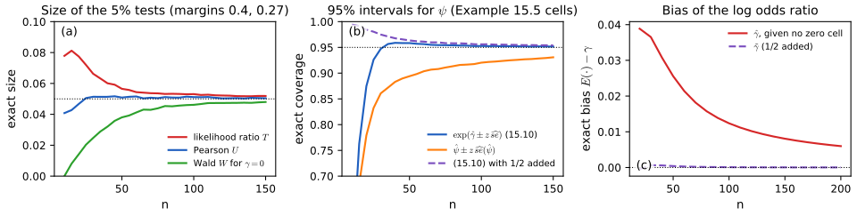
fig_15_s1. Download: PDF · SVGSee also: Chapter 10, Exercise 10.11 (an odds ratio interval for a drug trial) and Chapter 11, Exercise 11.4 (the log odds ratio, Bayesian and frequentist); Statistical Learning, logistic regression, whose slope for a binary input is \(\hgam\).
15.2 Two Discrete Variables
p. 243 Now \(Z\in\{1,\dots,I\}\) and \(Y\in\{1,\dots,J\}\), and the data form an \(I\times J\) table with \(X_{ij}\) the number of observations with \(Z=i\) and \(Y=j\). We test
\[ H_0:\ Y\indep Z\qquad\text{versus}\qquad H_1:\ Y\nindep Z. \tag{15.11} \]Theorem 15.9 (tests of independence for an I×J table) pp. 243–244, (15.12)–(15.13)
The likelihood ratio statistic for (15.11) is
\[ T=2\sum_{i=1}^I\sum_{j=1}^JX_{ij}\log\Big(\frac{X_{ij}X_{\cdot\cdot}}{X_{i\cdot}X_{\cdot j}}\Big), \tag{15.12} \]and Pearson's statistic is
\[ U=\sum_{i=1}^I\sum_{j=1}^J\frac{(X_{ij}-E_{ij})^2}{E_{ij}},\qquad E_{ij}=\frac{X_{i\cdot}X_{\cdot j}}{n}. \tag{15.13} \]Under \(H_0\), both converge in distribution to \(\chisq\nu\) with \(\nu=(I-1)(J-1)\).
Filling the gap 15.7: proof of Theorem 15.9, with the degrees of freedom derived pp. 243–244
Assume \(p_{ij}=a_ib_j\) with all \(a_i,b_j>0\). (a) The null MLE is \(\hat a_i\hat b_j=(X_{i\cdot}/n)(X_{\cdot j}/n)\), and (15.12) is twice the log likelihood ratio. (b) Parameter counting: \(IJ-1\) free parameters minus \((I-1)+(J-1)\) leaves \((I-1)(J-1)\). (c) The vector of Pearson residuals \(R_{ij}=(X_{ij}-E_{ij})/\sqrt{E_{ij}}\) converges to \(N(0,\Gamma)\) with
\[ \Gamma=(I_I-uu^\T)\otimes(I_J-vv^\T),\qquad u=(\sqrt{a_1},\dots,\sqrt{a_I})^\T,\quad v=(\sqrt{b_1},\dots,\sqrt{b_J})^\T, \]a projection of rank \((I-1)(J-1)\); hence \(U=\sum R_{ij}^2\convd\chisq{(I-1)(J-1)}\). (d) \(T-U\convp0\), so \(T\) has the same limit.
Proof
(a) As in Filling the gap 15.2: the null log-likelihood is \(\sum_iX_{i\cdot}\log a_i+\sum_jX_{\cdot j}\log b_j\), maximised by the observed margins, and \(T=2[\ell(\hat p)-\ell_0(\hat a,\hat b)]\) simplifies to (15.12).
(b) The full model has \(IJ\) probabilities with one constraint; the null model is parameterised by \(a\) (\(I-1\) free values) and \(b\) (\(J-1\)), through a smooth one-to-one map. Wilks' theorem (Theorem 10.22) then gives \(\chisq{(I-1)(J-1)}\) for \(T\). Part (c) proves the same limit for \(U\) directly.
(c) Let observation \(k\) have row indicator \(\rho_k\in\R^I\) and column indicator \(\kappa_k\in\R^J\) (each a vector with a single 1). Under \(H_0\), \(\rho_k\indep\kappa_k\), \(\E\rho_k=a\), \(\E\kappa_k=b\). With \(\hat a=\bar\rho\), \(\hat b=\bar\kappa\) and \(\hat P=n^{-1}\sum_k\rho_k\kappa_k^\T\) (the table of proportions), an exact algebraic identity holds:
\[ \hat P-\hat a\hat b^\T=\frac1n\sum_{k=1}^n(\rho_k-a)(\kappa_k-b)^\T-(\hat a-a)(\hat b-b)^\T. \](Expand both products: the terms \(\hat ab^\T\), \(a\hat b^\T\) and \(ab^\T\) cancel.) The matrices \(\xi_k=(\rho_k-a)(\kappa_k-b)^\T\) are iid with mean \(\E(\rho_k-a)\,\E(\kappa_k-b)^\T=0\) by independence, and the covariance of their vectorisation is, again by independence,
\[ \E\big[(\rho-a)(\rho-a)^\T\otimes(\kappa-b)(\kappa-b)^\T\big]=\Sigma_a\otimes\Sigma_b,\qquad\Sigma_a=\mathrm{diag}(a)-aa^\T,\ \Sigma_b=\mathrm{diag}(b)-bb^\T. \]By the multivariate CLT, \(n^{-1/2}\sum_k\xi_k\convd N(0,\Sigma_a\otimes\Sigma_b)\). The second term, multiplied by \(\sqrt n\), is \(\sqrt n(\hat a-a)\) (which converges in distribution, hence is bounded in probability) times \((\hat b-b)^\T\convp0\), so it tends to 0 in probability. Now
\[ R_{ij}=\frac{X_{ij}-n\hat a_i\hat b_j}{\sqrt{n\hat a_i\hat b_j}}=\frac{\sqrt n\,(\hat P_{ij}-\hat a_i\hat b_j)}{\sqrt{\hat a_i\hat b_j}}, \]and \(\sqrt{\hat a_i\hat b_j}\convp\sqrt{a_ib_j}\); by Slutsky's theorem the vector \(R\) converges to \(N(0,\Gamma)\) with \(\Gamma=D^{-1/2}(\Sigma_a\otimes\Sigma_b)D^{-1/2}\), \(D=\mathrm{diag}(a)\otimes\mathrm{diag}(b)\). The Kronecker product respects products, so
\[ \Gamma=\big(\mathrm{diag}(a)^{-1/2}\Sigma_a\,\mathrm{diag}(a)^{-1/2}\big)\otimes\big(\mathrm{diag}(b)^{-1/2}\Sigma_b\,\mathrm{diag}(b)^{-1/2}\big)=(I_I-uu^\T)\otimes(I_J-vv^\T), \]since \(\mathrm{diag}(a)^{-1/2}aa^\T\mathrm{diag}(a)^{-1/2}=uu^\T\). Each factor is the orthogonal projection onto the complement of a unit vector (\(\|u\|^2=\sum a_i=1\)), of rank \(I-1\) and \(J-1\). A Kronecker product of symmetric idempotent matrices is symmetric and idempotent, \((P\otimes Q)^2=P^2\otimes Q^2=P\otimes Q\), and its rank (its trace) is \(\mathrm{tr}P\cdot\mathrm{tr}Q=(I-1)(J-1)\). Finally, if \(V\sim N(0,\Pi)\) with \(\Pi\) a projection of rank \(r\), then \(\|V\|^2\sim\chisq r\) (write \(\Pi=QQ^\T\) with \(Q\) having \(r\) orthonormal columns: \(V\) has the law of \(QW\), \(W\sim N(0,I_r)\), and \(\|QW\|^2=\|W\|^2\); see also Filling the gap 10.9). The continuous mapping theorem gives \(U=\|R\|^2\convd\chisq{(I-1)(J-1)}\).
(d) The Taylor argument of Filling the gap 15.3(c) works for any \(I\times J\) table: the linear terms sum to zero because \(E\) and \(X\) have the same margins, and the cubic remainder is \(O_P(n^{-1/2})\) because \(X_{ij}-E_{ij}=\sqrt{E_{ij}}R_{ij}=O_P(\sqrt n)\). ∎
The rank deficiency has a plain meaning: the residual table has zero row sums and zero column sums when each residual is weighted by \(\sqrt{E_{ij}}\), and these \(I+J-1\) independent linear constraints leave \(IJ-(I+J-1)=(I-1)(J-1)\) free directions. The covariance \(\Gamma\) and the convergence of the simulated residual covariance to it were confirmed numerically (maximum deviation 0.04 at \(n=20{,}000\) for a \(3\times4\) table). For the same result proved through correspondence analysis, see Statistical Methods for Modern Biology, Filling the gap 9.10.
Example 15.10 (Hodgkin's disease: histology and response) p. 244
Patients with Hodgkin's disease (Dunsmore et al., 1987), classified by histological type and by response to treatment:
| type | positive | partial | none | total |
|---|---|---|---|---|
| LP | 74 | 18 | 12 | 104 |
| NS | 68 | 16 | 12 | 96 |
| MC | 154 | 54 | 58 | 266 |
| LD | 18 | 10 | 44 | 72 |
\(U=75.89\) and \(T=68.30\), each on \((4-1)(3-1)=6\) degrees of freedom, with p-values \(2.5\times10^{-14}\) and \(9.1\times10^{-13}\): response and histological type are strongly associated. The smallest expected count is 13.1, so the \(\chi^2\) approximation is safe.
Filling the gap 15.8: where is the association? Adjusted residuals p. 244
A significant test says that independence fails, not how. Under \(H_0\) the Pearson residual \(R_{ij}\) has limiting variance \((1-a_i)(1-b_j)\), not 1, so the adjusted residual
\[ \tilde R_{ij}=\frac{X_{ij}-E_{ij}}{\sqrt{E_{ij}(1-\hat a_i)(1-\hat b_j)}} \]is approximately \(N(0,1)\) for each cell, and cells with \(|\tilde R_{ij}|\) above 2 or 3 show where the table departs from independence.
Proof and the example
The diagonal entry of \(\Gamma=(I-uu^\T)\otimes(I-vv^\T)\) for cell \((i,j)\) is \((1-u_i^2)(1-v_j^2)=(1-a_i)(1-b_j)\) (Filling the gap 15.7(c)), so \(R_{ij}\convd N(0,(1-a_i)(1-b_j))\); dividing by the consistent estimate \(\sqrt{(1-\hat a_i)(1-\hat b_j)}\) gives \(N(0,1)\) by Slutsky's theorem. ∎
In Example 15.10 the adjusted residuals are \(+8.1\) for (LD, no response) and \(-6.2\) for (LD, positive response), with \(+2.9\) and \(+2.7\) for positive response in types LP and NS (Figure 15.S2(a)): the association is mostly that lymphocyte-depleted (LD) disease responds badly. With 12 cells, a few residuals beyond 2 are expected by chance alone; values of 6 to 8 are not. The squared Pearson residuals add up to \(U\); correspondence analysis (Statistical Methods for Modern Biology, Filling the gap 9.8) decomposes \(U/n\) into the squared singular values of the residual table to display the same pattern in a plane.
Small expected counts. Theorem 15.9 is a large-sample result. When expected counts are small the \(\chi^2\) approximation can be poor, and the remedy is to compute the null distribution directly: simulate tables under independence, either from the fitted model (multinomial with \(\hat a_i\hat b_j\)) or by permuting the column labels of the \(n\) individuals, which fixes both margins and gives the exact conditional null distribution (Fisher's exact test generalises this to any \(I\times J\) table). For a sparse \(3\times3\) table with \(n=25\) and every expected count below 5, \(U=6.87\) has \(\chi^2_4\) p-value 0.143 and permutation p-value 0.163, while \(T=6.22\) has \(\chi^2_4\) p-value 0.183 but permutation p-value 0.268 (Figure 15.S2(c)): Pearson's statistic is closer to its limit, as in the \(2\times2\) case.
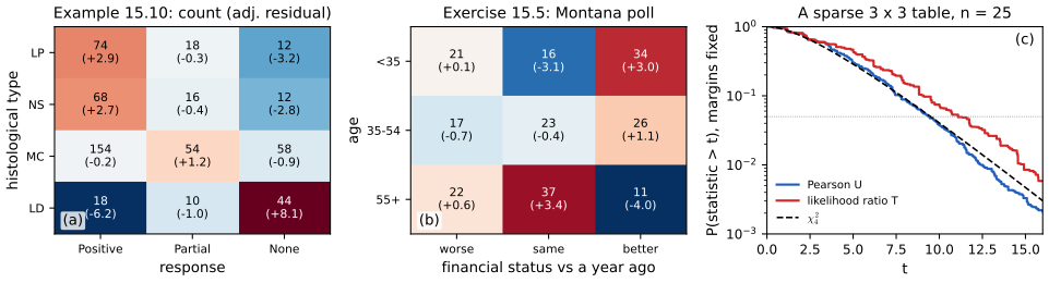
fig_15_s2. Download: PDF · SVGSee also: Statistical Methods for Modern Biology, two categorical variables and the correspondence analysis demo; Statistical Learning, association rules and their lift (Definition 14.1): a lift of 1 is the independence of two items.
15.3 Two Continuous Variables
p. 244 If \((Y,Z)\) is bivariate Normal, dependence is measured by the correlation \(\rho\), and tests, estimates and intervals for \(\rho\) are those of Section 14.2 of the book: the sample correlation \(r=\hat\rho\) (the plug-in estimator of Example 7.13) and Fisher's interval, which transforms by \(f(r)=\tfrac12\log\{(1+r)/(1-r)\}=\operatorname{arctanh}r\), uses the standard error \(1/\sqrt{n-3}\), and transforms back. Without Normality, the book notes, the same methods give inferences about \(\rho\), but \(\rho=0\) no longer implies independence; the converse remains true: correlated variables are dependent.
Filling the gap 15.9: correlation and independence, and testing one with the other p. 244
Assume \(0<\V(Y),\V(Z)<\infty\). (a) If \(Y\indep Z\) then \(\rho=0\); hence \(\rho\ne0\) implies dependence. (b) The converse fails, even when both margins are Normal: with \(Z\sim N(0,1)\) and an independent random sign \(S=\pm1\), \(Y=SZ\) is \(N(0,1)\), \(\Corr(Y,Z)=0\), yet \(|Y|=|Z|\). (c) If \((Y,Z)\) is bivariate Normal, \(\rho=0\) does imply independence. (d) The key fact for testing. If \(Y\indep Z\), whatever their distributions, \(\sqrt n\,r\convd N(0,1)\). So "reject when \(\sqrt n|r|>z_{\alpha/2}\)", or its Fisher version \(\sqrt{n-3}\,|\operatorname{arctanh}r|>z_{\alpha/2}\), is an asymptotically level \(\alpha\) test of independence for any distribution with finite variances. (e) It is not a valid test of \(\rho=0\) when the variables are dependent but uncorrelated: in general \(\sqrt n\,r\convd N(0,\E[\tilde Y^2\tilde Z^2])\) with \(\tilde Y,\tilde Z\) the standardised variables, and for the pair of (b) the variance is 3, so the 5% test rejects with probability tending to \(2\Phi(-1.96/\sqrt3)=0.258\). (f) For bivariate Normal data, \(\sqrt n(r-\rho)\convd N(0,(1-\rho^2)^2)\), and \(\operatorname{arctanh}\) is exactly the transformation that makes the variance free of \(\rho\): \(\sqrt n(\operatorname{arctanh}r-\operatorname{arctanh}\rho)\convd N(0,1)\). (g) Under bivariate Normal independence, \(t=r\sqrt{n-2}/\sqrt{1-r^2}\) has exactly the \(t_{n-2}\) distribution.
Proof
(a) Independence gives \(\E(YZ)=\E Y\,\E Z\) (Result 3.4), so the covariance is 0. The contrapositive is the second statement.
(b) By symmetry of \(Z\),
\[ \P(SZ\le y)=\tfrac12\P(Z\le y)+\tfrac12\P(-Z\le y)=\Phi(y). \]Also \(\Cov(Y,Z)=\E(SZ^2)=\E S\,\E Z^2=0\). But
\[ \P(|Y|\le1,|Z|>1)=0\ne\P(|Y|\le1)\,\P(|Z|>1). \]So the pair is not jointly Normal: joint Normality is a property of the pair, not of the margins (Filling the gap 3.3 gives other examples).
(c) With \(\rho=0\) the bivariate Normal density \(f(y,z)\) has a diagonal covariance matrix and factorises into the two Normal margins, which is independence (Result 2.11).
(d) and (e). Standardise: \(\tilde Y=(Y-\mu_Y)/\sigma_Y\), \(\tilde Z=(Z-\mu_Z)/\sigma_Z\); \(r\) is unchanged. Write
\[ r=\frac{\overline{\tilde Y\tilde Z}-\overline{\tilde Y}\,\overline{\tilde Z}}{\sqrt{(\overline{\tilde Y^2}-\overline{\tilde Y}^2)(\overline{\tilde Z^2}-\overline{\tilde Z}^2)}}. \]When \(\rho=0\), \(\E(\tilde Y\tilde Z)=0\), and if also \(\E[\tilde Y^2\tilde Z^2]<\infty\) the CLT gives \(\sqrt n\,\overline{\tilde Y\tilde Z}\convd N(0,\E[\tilde Y^2\tilde Z^2])\). The correction \(\sqrt n\,\overline{\tilde Y}\,\overline{\tilde Z}\) is \(O_P(1)\cdot o_P(1)\to0\), and the denominator tends to 1 in probability (law of large numbers), so by Slutsky \(\sqrt n\,r\convd N(0,\E[\tilde Y^2\tilde Z^2])\). Under independence \(\E[\tilde Y^2\tilde Z^2]=\E\tilde Y^2\,\E\tilde Z^2=1\) (finite whenever the variances are), which is (d); since \(\sqrt{n-3}\operatorname{arctanh}r=\sqrt n\,r\,(1+o_P(1))\), the Fisher version has the same limit. For \(Y=SZ\), \(\E[\tilde Y^2\tilde Z^2]=\E[Z^4]=3\), which is (e). This is the influence-function variance of Filling the gap 7.10 evaluated at \(\rho=0\).
(f) The general influence-function variance of \(r\) is \(\E\big[(\tilde Y\tilde Z-\tfrac\rho2(\tilde Y^2+\tilde Z^2))^2\big]\) (Filling the gap 7.10). For the bivariate Normal, \(\E\tilde Y^4=3\), \(\E\tilde Y^3\tilde Z=3\rho\) and \(\E\tilde Y^2\tilde Z^2=1+2\rho^2\) (Isserlis' theorem), so it equals
\[ (1+2\rho^2)-\rho(3\rho+3\rho)+\frac{\rho^2}4\big(3+3+2(1+2\rho^2)\big)=1-2\rho^2+\rho^4=(1-\rho^2)^2. \]With \(f(\rho)=\operatorname{arctanh}\rho\), \(f'(\rho)=1/(1-\rho^2)\), and the delta method gives the variance \(f'(\rho)^2(1-\rho^2)^2=1\). The refinement \(1/(n-3)\) in place of \(1/n\) comes from the next terms of the expansion (Fisher, 1921; Hotelling, 1953); in a simulation with \(n=20\) and \(\rho=0.6\), \(\sqrt{17}(\operatorname{arctanh}r-\operatorname{arctanh}\rho)\) had standard deviation 1.01.
(g) Condition on \(Z_1,\dots,Z_n\). Under independence the \(Y_i\) are still iid \(N(\mu,\sigma^2)\), so the simple linear regression of \(Y\) on \(Z\) satisfies the Normal linear model with true slope 0, and its slope \(t\)-statistic has the \(t_{n-2}\) distribution. Algebraically that statistic equals \(r\sqrt{n-2}/\sqrt{1-r^2}\) (the slope is \(r\,s_Y/s_Z\) and the residual sum of squares is \((1-r^2)\sum(Y_i-\bar Y)^2\)). The conditional law does not depend on the \(Z\) values, so it is also the unconditional law. ∎
Rank methods. Replacing the observations by their ranks gives Spearman's rank correlation, and counting concordant minus discordant pairs gives Kendall's \(\tau\). Under independence the ranks of the \(Y\)'s are a uniformly random permutation of the ranks of the \(Z\)'s, so the null distribution of either statistic is the same for every pair of continuous distributions, and the permutation test built on it is exact (Section 10.5). These tests detect monotone dependence; none of the three detects the dependence of (b), which has no monotone trend at all.
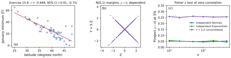
fig_15_s3. Download: PDF · SVGSee also: Chapter 7, the standard error of the sample correlation and the plug-in functionals demo for the correlation of the Old Faithful data.
15.4 One Continuous Variable and One Discrete
pp. 244–245 Let \(Y\in\{1,\dots,I\}\) be discrete and \(Z\) continuous, and let \(F_i(z)=\P(Z\le z\given Y=i)\) be the conditional cdf of \(Z\) in group \(i\).
Theorem 15.11 (independence means equal conditional distributions) p. 245
If \(\P(Y=i)>0\) for every \(i\), then \(Y\indep Z\) if and only if \(F_1=\dots=F_I\).
Filling the gap 15.10: proof of Theorem 15.11 p. 245
One direction is immediate; for the other, equality of the conditional cdfs gives the factorisation \(\P(Z\le z,Y=i)=\P(Z\le z)\P(Y=i)\), and a factorisation on half-lines extends to all Borel sets.
Proof
Write \(\pi_i=\P(Y=i)>0\) (needed for \(F_i\) to be defined). If \(Y\indep Z\), then \(F_i(z)=\P(Z\le z,Y=i)/\pi_i=\P(Z\le z)\) for every \(i\): all \(F_i\) equal the marginal cdf.
Conversely, let \(F_i=F\) for all \(i\). By the law of total probability \(\P(Z\le z)=\sum_i\pi_iF_i(z)\), which is \(F(z)\), so
\[ \P(Z\le z,Y=i)=\pi_iF(z)=\P(Y=i)\,\P(Z\le z)\quad\text{for all }z,i. \]Fix \(i\). The two finite measures \(\mu_1(A)=\P(Z\in A,Y=i)\) and \(\mu_2(A)=\pi_i\P(Z\in A)\) on the Borel sets agree on the half-lines \((-\infty,z]\), which form a class closed under intersection that generates the Borel \(\sigma\)-field, and on \(\R\) itself; by Dynkin's \(\pi\)-\(\lambda\) theorem they agree on every Borel set. Summing over \(i\in B\) gives \(\P(Z\in A,Y\in B)=\P(Z\in A)\P(Y\in B)\) for all \(A\) and \(B\). ∎
Continuity of \(Z\) is not used: the theorem holds for any real \(Z\).
p. 245 So testing independence means testing \(H_0:F_1=\dots=F_I\). For \(I=2\), with \(n_1\) and \(n_2\) observations in the two groups, let
\[ \Fh_1(z)=\frac1{n_1}\sum_{k=1}^n\I(Z_k\le z)\I(Y_k=1),\qquad\Fh_2(z)=\frac1{n_2}\sum_{k=1}^n\I(Z_k\le z)\I(Y_k=2) \]be the two empirical cdfs, and use the two-sample Kolmogorov-Smirnov statistic \(D=\sup_x|\Fh_1(x)-\Fh_2(x)|\).
Theorem 15.12 (Kolmogorov-Smirnov limit) p. 245, (15.14)
Let
\[ H(t)=1-2\sum_{j=1}^\infty(-1)^{j-1}e^{-2j^2t^2}. \tag{15.14} \]Under \(H_0:F_1=F_2\), with \(F_1\) continuous and \(n_1,n_2\to\infty\),
\[ \P\Big(\sqrt{\tfrac{n_1n_2}{n_1+n_2}}\,D\le t\Big)\to H(t). \]So rejecting when \(\sqrt{n_1n_2/(n_1+n_2)}\,D>H^{-1}(1-\alpha)\) is an approximate level \(\alpha\) test; \(H^{-1}(0.95)=1.358\).
Filling the gap 15.11: the exact null distribution of \(D\), and a proof of Kolmogorov's limit p. 245
(a) Distribution-free. Under \(H_0\) with a continuous common cdf, the law of \(D\) depends only on \(n_1,n_2\): it is the law of \(\max_{(i,j)}|i/n_1-j/n_2|\) along a uniformly random lattice path from \((0,0)\) to \((n_1,n_2)\). (b) Exact computation. A recursion over the \((n_1+1)(n_2+1)\) lattice points gives \(\P(D\ge d)\) exactly. (c) Equal sizes, closed form (Gnedenko and Korolyuk, 1951). For \(n_1=n_2=n\) and integers \(m\ge1\),
\[ \P\Big(D\ge\frac mn\Big)=\frac2{\binom{2n}n}\sum_{j\ge1}(-1)^{j-1}\binom{2n}{n-jm}. \](d) The limit. For \(n_1=n_2=n\to\infty\), (c) converges to \(1-H(t)\). (e) For unequal sizes the same limit holds by the functional central limit theorem. (f) Ties. For discrete data the test that uses the continuous-data null law is conservative; the permutation distribution of \(D\) is exact in all cases.
Proof
(a) Under \(H_0\), given the group sizes, \(Z_1,\dots,Z_n\) are iid with continuous cdf \(F\), so there are no ties with probability 1 and, by exchangeability, every assignment of the \(n_1\) group-1 labels to the positions of the sorted pooled sample is equally likely: \(\binom n{n_1}\) arrangements, each with probability \(1/\binom n{n_1}\). Walk through the sorted pooled sample, stepping right for a group-1 value and up for a group-2 value; after reaching the point \((i,j)\) we have passed \(i\) values of group 1 and \(j\) of group 2, so \(\Fh_1-\Fh_2=i/n_1-j/n_2\) at that pooled value, and these are the only values the difference takes. Hence \(D\,n_1n_2=\max|in_2-jn_1|\) over the path, a function of the arrangement alone, and \(F\) has disappeared.
(b) A uniformly random arrangement can be generated step by step: at \((i,j)\), the next value belongs to group 1 with probability \((n_1-i)/(n-i-j)\), the fraction of group-1 values among those not yet placed (drawing without replacement). Let \(P(i,j)\) be the probability of reaching \((i,j)\) with \(|i'n_2-j'n_1|<K\) at every point visited so far. Then \(P(0,0)=1\),
\[ P(i,j)=P(i-1,j)\,\frac{n_1-i+1}{n-i-j+1}+P(i,j-1)\,\frac{n_2-j+1}{n-i-j+1} \]for points inside the band, and the probability that falls on a point with \(|in_2-jn_1|\ge K\) is added to \(\P(Dn_1n_2\ge K)\). This is ks_exact_sf; it agrees with scipy's exact two-sample p-values to \(10^{-9}\).
(c) With \(n_1=n_2=n\), let \(S_k\) be (number of group-1 values) minus (number of group-2 values) among the first \(k\) pooled values: a path of \(2n\) steps \(\pm1\) from 0 to 0, all \(\binom{2n}n\) such bridges equally likely, and \(D=\max_k|S_k|/n\). Fix \(m\ge1\). Reflection. The bridges that reach level \(m\) are in one-to-one correspondence with all \(\pm1\) paths of length \(2n\) from 0 to \(2m\): reflect the part after the first visit to \(m\) about \(m\) (and back again for the inverse). Those paths have \(n+m\) up-steps, so there are \(\binom{2n}{n+m}=\binom{2n}{n-m}\) of them. Alternating visits. Let \(A_j\) be the set of bridges that visit \(m\), later \(-m\), later \(m\), and so on, \(j\) alternating visits starting with \(m\); let \(B_j\) be the same starting with \(-m\). Reflecting successively after the first visits to \(m,3m,\dots,(2j-1)m\) maps \(A_j\) one-to-one onto the paths from 0 to \(2jm\) (a later visit to \(-m\) becomes a visit to \(3m\) after the first reflection, and so on), so \(|A_j|=|B_j|=\binom{2n}{n-jm}\). Inclusion-exclusion. For a bridge, let \(L\) be the length of its greedy sequence of alternating barrier visits (the first visit to either barrier, then the first later visit to the other one, and so on). The greedy choice is optimal, so the longest alternating chain starting with the barrier visited first has length \(L\) and the longest starting with the other barrier has length \(L-1\). Hence
\[ \sum_{j\ge1}(-1)^{j-1}\big(\I_{A_j}+\I_{B_j}\big)=\sum_{j=1}^{L}(-1)^{j-1}+\sum_{j=1}^{L-1}(-1)^{j-1}=\begin{cases}1&L\ge1\\0&L=0,\end{cases} \]because the two alternating sums have lengths of different parity, one equal to 1 and the other to 0. The left side is therefore the indicator of \(\max_k|S_k|\ge m\). Summing over all bridges and dividing by \(\binom{2n}n\) gives (c). The formula agrees with the recursion (b) for all \(n\le25\).
(d) Fix \(t>0\) and let \(m=\lceil t\sqrt{2n}\rceil\), so that \(\{\sqrt{n/2}\,D\ge t\}=\{\max|S_k|\ge m\}\) (because \(\sqrt{n/2}\,D=\max|S_k|/\sqrt{2n}\)). For \(0\le k\le n\),
\[ \frac{\binom{2n}{n-k}}{\binom{2n}n}=\prod_{i=1}^k\frac{n-i+1}{n+i}=\prod_{i=1}^k\Big(1-\frac{2i-1}{n+i}\Big). \]Using \(\log(1-x)=-x+O(x^2)\) and \((2i-1)/(n+i)=(2i-1)/n+O(i^2/n^2)\), the logarithm equals \(-k^2/n+O(k^3/n^2+k/n)\), which for \(k=jm\) with \(m\sim t\sqrt{2n}\) tends to \(-2j^2t^2\). Each term of (c) therefore converges to \(2(-1)^{j-1}e^{-2j^2t^2}\). For domination, \(1-x\le e^{-x}\) and \(n+i\le2n\) give \(\binom{2n}{n-k}/\binom{2n}n\le e^{-k^2/(2n)}\le e^{-j^2t^2}\) when \(k=jm\ge jt\sqrt{2n}\), and \(\sum_je^{-j^2t^2}<\infty\). By dominated convergence for series,
\[ \P\big(\sqrt{n/2}\,D\ge t\big)\to2\sum_{j\ge1}(-1)^{j-1}e^{-2j^2t^2}=1-H(t). \]Since \(H\) is continuous, the same limit holds for \(\P(\sqrt{n/2}\,D>t)\), which is Theorem 15.12 for \(n_1=n_2\). Numerically, at \(n=5000\) the exact probabilities are within 0.01 of the limit for \(t\) between 0.6 and 1.8.
(e) For unequal sizes, by Donsker's theorem (Billingsley, 1999; van der Vaart, 1998, Chapter 19) \(\sqrt{n_1}(\Fh_1-F)\) and \(\sqrt{n_2}(\Fh_2-F)\) converge jointly to \(B_1\circ F\) and \(B_2\circ F\) with \(B_1,B_2\) independent Brownian bridges (the covariance \(\min(u,v)-uv\) computed in Chapter 7). If \(n_1/n\to\lambda\in(0,1)\),
\[ \sqrt{\tfrac{n_1n_2}n}\,(\Fh_1-\Fh_2)=\sqrt{\tfrac{n_2}n}\,\sqrt{n_1}(\Fh_1-F)-\sqrt{\tfrac{n_1}n}\,\sqrt{n_2}(\Fh_2-F)\convd\big(\sqrt{1-\lambda}\,B_1-\sqrt\lambda\,B_2\big)\circ F, \]and \(\sqrt{1-\lambda}B_1-\sqrt\lambda B_2\) is a Gaussian process with covariance \((1-\lambda+\lambda)(\min(u,v)-uv)\): again a Brownian bridge \(B\). For continuous \(F\), \(\sup_x|B(F(x))|=\sup_{u}|B(u)|\), whose distribution is \(H\) (Kolmogorov, 1933); by (d) this is the same \(H\) obtained from the equal-size case. Because the limit does not depend on \(\lambda\), a subsequence argument removes the assumption that \(n_1/n\) converges: \(\min(n_1,n_2)\to\infty\) suffices. Both sizes must grow: with \(n_1\) fixed the limit is a different distribution.
(f) If \(F\) has atoms, write \(Z_k=F^{-1}(U_k)\) with \(U_k\) iid uniform. \(F^{-1}\) is non-decreasing, so the empirical cdfs of the \(Z\)'s are those of the \(U\)'s evaluated only at the points \(F(x)\), and \(D(Z)\le D(U)\): the statistic is stochastically smaller than under continuity, and using the continuous-data critical value is conservative. The permutation test (shuffle the group labels over the observed pooled values, Section 10.5) is exact whether or not there are ties. ∎
How good is \(H\) for moderate samples? The exact size of the test "reject when the scaled statistic exceeds \(H^{-1}(0.95)\)" never exceeds 0.05 for \(n_1=n_2\) up to 120 or for \(n_2=2n_1\), and oscillates between about 0.02 and 0.05 because \(D\) is discrete (Figure 15.S4(c)); the test is slightly conservative. For more than two groups, the same idea leads to \(k\)-sample versions (Kiefer, 1959), or to pairwise comparisons with a multiple-testing correction.
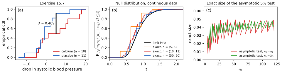
fig_15_s4. Download: PDF · SVGSee also: the one-sample Kolmogorov-Smirnov distance, the DKW band and Kolmogorov's limit in Chapter 7 (Theorem 7.5, Filling the gap 7.5, the DKW band demo); Statistical Methods for Modern Biology, Filling the gap 3.7 and the empirical cdf demo.
15.5 Appendix
pp. 245–246 Odds. The odds of an event \(A\) are \(\odds(A)=\P(A)/(1-\P(A))\), and \(\P(A)=\odds(A)/(1+\odds(A))\). Let \(E\) be exposure (to smoking, radiation, ...) and \(D\) disease. The odds ratio
\[ \psi=\frac{\odds(D\given E)}{\odds(D\given E^c)} \]equals 1 exactly when disease and exposure are independent. With rows \(E^c,E\) and columns \(D^c,D\), so that \(p_{11}=\P(E,D)\), we have \(\P(D\given E)=p_{11}/(p_{10}+p_{11})\), \(\P(D\given E^c)=p_{01}/(p_{00}+p_{01})\), \(\odds(D\given E)=p_{11}/p_{10}\), \(\odds(D\given E^c)=p_{01}/p_{00}\), and therefore \(\psi=p_{00}p_{11}/(p_{01}p_{10})\), Definition 15.1 again.
pp. 246–248 Three ways to collect the data. (i) Multinomial (cross-sectional) sampling: a random sample of \(n\) people, each classified by exposure and disease; \(X\sim\Mult(n,p)\) and \(\hpsi=X_{00}X_{11}/(X_{01}X_{10})\). (ii) Prospective (cohort) sampling: fixed numbers \(x_{0\cdot}\) unexposed and \(x_{1\cdot}\) exposed people are followed, and the numbers who fall ill are \(X_{01}\sim\Bin(x_{0\cdot},r_0)\) and \(X_{11}\sim\Bin(x_{1\cdot},r_1)\), with \(r_0=\P(D\given E^c)\), \(r_1=\P(D\given E)\); the cell probabilities are not all estimable, but \(\psi\) is a function of \(r_1\) and \(r_0\), and plugging in \(X_{11}/X_{1\cdot}\) and \(X_{01}/X_{0\cdot}\) gives the same \(\hpsi\). (iii) Case-control (retrospective) sampling: fixed numbers of diseased (cases) and healthy people (controls), each asked about past exposure; with \(e_0=\P(E\given D^c)\) and \(e_1=\P(E\given D)\), the exposed counts are \(X_{10}\sim\Bin(X_{\cdot0},e_0)\) and \(X_{11}\sim\Bin(X_{\cdot1},e_1)\). This is far more efficient for a rare disease. Surprisingly, \(\psi\) is still estimable, because
\[ \frac{\odds(E\given D)}{\odds(E\given D^c)}=\frac{p_{11}/p_{01}}{p_{10}/p_{00}}=\psi, \]and the estimate is once more \(X_{00}X_{11}/(X_{01}X_{10})\). The risk difference \(r_1-r_0\) is not estimable from a case-control study, since by Bayes' theorem it involves \(\P(D)\), which the design fixes arbitrarily. The relative risk \(\xi=r_1/r_0\) is not estimable either, but it is close to \(\psi\) for a rare disease:
Theorem 15.13 (the rare disease assumption) p. 248
Let \(\xi=\P(D\given E)/\P(D\given E^c)\). Then \(\psi/\xi\to1\) as \(\P(D)\to0\) (with the exposure probability \(\P(E)\) held fixed in \((0,1)\); see below).
Filling the gap 15.12: the three designs, non-estimability, and a proof of Theorem 15.13 with its missing condition pp. 246–248
(a) In all three designs \(\hpsi=X_{00}X_{11}/(X_{01}X_{10})\), its standard error is (15.7), and the tests of Section 15.1 are valid (Filling the gaps 15.2 and 15.4(d)). (b) In a case-control design the risk difference is not identified: two populations with the same \(\P(E\given D)\) and \(\P(E\given D^c)\), and so the same distribution of the data, can have different risk differences. (c) Exactly,
\[ \frac\psi\xi=\frac{1-\P(D\given E^c)}{1-\P(D\given E)}. \]So \(\psi/\xi\to1\) whenever both conditional risks tend to 0, which follows from \(\P(D)\to0\) if \(\P(E)\) stays bounded away from 0 and 1. Without that condition the theorem can fail. (d) When the disease is rare, case-control sampling estimates \(\psi\) with far smaller variance than the other designs of the same size.
Proof
(a) The estimates were derived above; the standard error and the tests were treated in the cited boxes, each for fixed row or fixed column totals.
(b) In a case-control study the data distribution depends only on \(\P(E\given D)=e_1\) and \(\P(E\given D^c)=e_0\). By Bayes' theorem, with \(\delta=\P(D)\) and \(\P(E)=e_1\delta+e_0(1-\delta)\),
\[ \P(D\given E)-\P(D\given E^c)=\frac{e_1\delta}{e_1\delta+e_0(1-\delta)}-\frac{(1-e_1)\delta}{(1-e_1)\delta+(1-e_0)(1-\delta)}, \]which varies with \(\delta\). For example, with \(e_1=0.4\) and \(e_0=0.25\) the risk difference is 0.008 when \(\delta=0.01\) and 0.119 when \(\delta=0.2\): the same data distribution, two different answers.
(c) With \(r_1=\P(D\given E)\) and \(r_0=\P(D\given E^c)\), \(\psi=\{r_1/(1-r_1)\}/\{r_0/(1-r_0)\}\) and \(\xi=r_1/r_0\), so \(\psi/\xi=(1-r_0)/(1-r_1)\). If \(c\le\P(E)\le1-c\) for some \(c>0\), then
\[ \P(D)=r_1\P(E)+r_0\P(E^c)\ge c\max(r_1,r_0), \]so \(\P(D)\to0\) forces \(r_0,r_1\to0\) and \(\psi/\xi\to1\); quantitatively, for \(\P(D)<c\),
\[ \Big|\frac\psi\xi-1\Big|\le\frac{\max(r_0,r_1)}{1-r_1}\le\frac{\P(D)}{c-\P(D)}. \]Counterexample without the condition: take \(r_1=1/2\) and \(\P(E)=r_0=\varepsilon\). Then \(\P(D)=\varepsilon/2+\varepsilon(1-\varepsilon)\to0\), but \(\psi/\xi=(1-\varepsilon)/(1/2)\to2\). The condition is natural (it says the exposure is not itself vanishingly rare), but it is needed.
(d) By (15.7) the variance of \(\hgam\) is about \(\sum1/\E X_{ij}\), dominated by the smallest expected cell. In a cross-sectional or cohort study of a rare disease the diseased cells are tiny (with \(\P(D\given E^c)=0.01\), \(\psi=2\), \(\P(E)=0.4\) and \(n=646\), about 4 unexposed and 5 exposed cases are expected); a case-control study with 174 cases and 472 controls has no small cell. In a simulation of 20,000 studies of each kind from this population (Figure 15.S5(b)), the standard deviation of the corrected log odds ratio was 0.72 (multinomial), 0.73 (cohort of 323 + 323) and 0.18 (case-control), the last matching \(\sqrt{\sum1/\E X_{ij}}=0.180\) for the case-control design. ∎
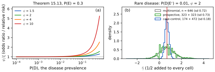
fig_15_s5. Download: PDF · SVGNotes on the book
One slip of Chapter 15 is in the author's errata lists; the other points are mine, each with its evidence. All the numbers of Examples 15.5, 15.8 and 15.10 were recomputed and are correct.
Page 245, line −2: "as" should be "has"
"Suppose event \(A\) as probability \(\P(A)\)" should read "has probability". Listed in the author's errata.
Page 240: the indices of \(X_{ij}\)
The text defines \(X_{ij}\) as the number of observations with \(Y=i\) and \(Z=j\), but the table above it puts rows for \(Z\) and columns for \(Y\), and \(p_{ij}\) is defined as \(\P(Z=i,Y=j)\). Section 15.2 uses "\(Z=i\) and \(Y=j\)", which matches the tables. Nothing depends on it, because independence is symmetric and \(\psi\) is unchanged by transposing the table. Not in the errata lists.
Pages 240, 245 and 248: three missing conditions
Theorem 15.2 needs \(p_{01}p_{10}>0\) (better, all cells positive) for \(\psi\) to be defined (Filling the gap 15.1). Theorem 15.11 needs \(\P(Y=i)>0\) for \(F_i\) to be defined. Theorem 15.12 needs a continuous common cdf and both \(n_1\) and \(n_2\) to grow; "\(n\to\infty\)" alone allows one group to stay small, and with ties the limit law is stochastically smaller (Filling the gap 15.11(e)–(f)). Theorem 15.13 needs \(\P(E)\) to stay away from 0 and 1; a counterexample is in Filling the gap 15.12(c). Not in the errata lists.
Pages 242–243, Example 15.8: "twice as likely" and the factor 2
The book concludes that "tonsillectomy patients were twice as likely to have Hodgkin's disease". The estimate is an odds ratio from a case-control study, in which \(\P(D\given E)\) is not estimable (Section 15.5); a statement about likelihoods (a relative risk) follows only through the rare-disease approximation of Theorem 15.13, plausible here but not stated. What the data say directly is that the odds of a past tonsillectomy were twice as high among the cases as among the controls. Also, the intervals use 2 in place of \(z_{0.025}=1.96\); with 1.96 the interval for \(\psi\) is \((1.40,2.84)\) rather than \((1.39,2.86)\). Not in the errata lists.
Page 244, Section 15.3: Fisher's interval without Normality, and "than"
The book says that without Normality "we can still use the methods in Section 14.2 to draw inferences about the correlation". The standard error \(1/\sqrt{n-3}\) of Fisher's method is derived for bivariate Normal data; for other distributions the asymptotic variance of \(\sqrt n(r-\rho)\) is the influence-function variance of Filling the gap 7.10, which can be very different (for the uncorrelated pair \(Y=SZ\) of Filling the gap 15.9 it is 3 instead of 1, and the nominal 5% test rejects 25.8% of the time, Figure 15.S3(c)). The methods remain valid as tests of independence, and a bootstrap interval (Chapter 8) is the safe choice for \(\rho\). In the same paragraph, "correlated than we can conclude" should read "then". Not in the errata lists.
15.6 Exercises
All seven exercises of Chapter 15 (Wasserman, 2004, pp. 248–249), restated in my own words, with complete solutions (hidden). Computational answers come from the chapter code (functions ex4 to ex7). The data sets of Exercises 15.5 to 15.7 are the book's montana.dat, temp.dat and calcium.dat, from the book's website.
Exercise 15.1. Prove Theorem 15.2.
Solution
See Filling the gap 15.1. The identity \(p_{00}p_{11}-p_{01}p_{10}=p_{00}-p_{0\cdot}p_{\cdot0}\) shows that \(\psi=1\) if and only if the cell \((0,0)\) factorises; for binary variables one factorised cell forces the other three, which is independence; and \(\gamma=0\iff\psi=1\).
Exercise 15.2. Prove Theorem 15.3.
Solution
See Filling the gap 15.2: under independence the log-likelihood splits into two multinomial log-likelihoods, maximised by the observed margins, so the null MLE is \(\hat p^0_{ij}=X_{i\cdot}X_{\cdot j}/n^2\); twice the log of the likelihood ratio is (15.4); the models have 3 and 2 free parameters, so Wilks' theorem gives \(\chisq1\). A direct proof of the limit, valid for any \(I\times J\) table, is Filling the gap 15.7.
Exercise 15.3. Prove Theorem 15.6.
Solution
See Filling the gap 15.4: equivariance of the MLE gives (15.6); the multivariate delta method with gradient \((1/p_{00},-1/p_{01},-1/p_{10},1/p_{11})\) and the multinomial covariance \(\mathrm{diag}(p)-pp^\T\) gives the asymptotic variance \(\sum_{ij}1/(np_{ij})\), estimated by \(\sum1/X_{ij}\), which is (15.7); the delta method for \(e^\gamma\) gives (15.8).
Exercise 15.4. A newspaper report on a study of death sentencing in Maryland gave (approximately) the following counts of murder cases by the race of the victim and the sentence. Analyse the data with the tools of this chapter, interpret the results, and explain why these data alone cannot support a causal conclusion.
death sentence no death sentence black victim 14 641 white victim 62 594 Solution
Rates. A death sentence was given in \(14/655=2.1\%\) of black-victim cases and \(62/656=9.5\%\) of white-victim cases.
Tests. \(T=34.53\) and \(U=32.10\) on 1 degree of freedom, p-values \(4\times10^{-9}\) and \(1.5\times10^{-8}\). The expected counts are all above 37, so the \(\chi^2\) approximation is reliable.
Odds ratio. \(\hpsi=(14\cdot594)/(641\cdot62)=0.209\) and \(\hgam=-1.564\), with
\[ \hse(\hgam)=\sqrt{\tfrac1{14}+\tfrac1{641}+\tfrac1{62}+\tfrac1{594}}=0.301, \]so \(W=-5.19\) (p-value \(2\times10^{-7}\)). 95% intervals: \((-2.155,-0.974)\) for \(\gamma\) and \((0.116,0.378)\) for \(\psi\) by (15.10). Equivalently, the odds of a death sentence were \(1/0.209=4.8\) times higher, with interval \((2.6,8.6)\), when the victim was white. Since death sentences are rare, the odds ratio is close to the ratio of rates, \(2.1/9.5=0.23\).
Interpretation. In these cases, the race of the victim and the sentence are strongly associated: a death sentence was about four to five times as frequent when the victim was white.
Why not causation. The cases differ in many ways besides the victim's race, and some of those ways affect the sentence: the circumstances of the crime (murders during another felony, multiple victims, other aggravating factors that make a case eligible for the death penalty), the county (prosecutors in different jurisdictions seek the death penalty at very different rates, and the racial make-up of victims differs between jurisdictions), the race and criminal record of the defendant, and the prosecutor's decision to seek a death sentence at all. Any of these could produce the association, or reverse it within subgroups (Simpson's paradox). A causal claim needs either randomisation, impossible here, or an analysis that adjusts for these confounders (Chapter 16 of the book), which is what the authors of the full study attempted with much more information. The counts are also, as the book notes, an approximate re-creation from a newspaper article.
Exercise 15.5. Analyse the relation between Age and Financial status in the Montana outlook poll (the book's
montana.dat).Solution
The poll asked a sample of Montana residents whether their personal finances were worse, the same or better than a year earlier. Dropping the 2 respondents with a missing answer leaves 207. The table (rows age under 35, 35 to 54, 55 and over; columns worse, same, better):
age worse same better total under 35 21 16 34 71 35 to 54 17 23 26 66 55 and over 22 37 11 70 \(U=20.68\) and \(T=22.06\) on \((3-1)(3-1)=4\) degrees of freedom, p-values 0.0004 and 0.0002; every expected count is at least 19.1, so the approximation is sound, and a permutation test agrees (no permutation in 2000 reaches the observed \(U\)). The adjusted residuals (Figure 15.S2(b)) locate the association: the under-35s answer "better" more often than independence predicts (\(+3.0\)) and "same" less often (\(-3.1\)); the over-55s answer "same" more often (\(+3.4\)) and "better" much less often (\(-4.0\)); the middle group is unremarkable. Younger respondents were more likely to report improving finances, older respondents stable ones. As always, this is an association in a survey, and age is entangled with income, employment and retirement.
Exercise 15.6. Estimate the correlation between January temperature and latitude for 56 US cities (the book's
temp.dat), with estimates, tests and confidence intervals.Solution
Estimate. \(r=-0.848\): cities further north have colder Januaries (Figure 15.S3(a)).
Tests of \(\rho=0\). The \(t\) statistic is \(t=r\sqrt{54}/\sqrt{1-r^2}=-11.76\) on 54 degrees of freedom, p-value \(1.6\times10^{-16}\); the Fisher statistic is \(\sqrt{53}\operatorname{arctanh}(r)=-9.09\); a permutation test with 10,000 shuffles finds nothing as extreme (p-value \(\le1/10001\)). Rank methods agree: Spearman's \(r_s=-0.815\), Kendall's \(\tau=-0.683\). By Filling the gap 15.9(d), these are valid tests of independence without any Normality assumption.
Intervals. Fisher: \(\operatorname{arctanh}(-0.848)=-1.250\), interval \(-1.250\pm1.96/\sqrt{53}\), transformed back: \((-0.908,-0.753)\). Delta method: \(r\pm1.96(1-r^2)/\sqrt{56}=(-0.922,-0.774)\). Bootstrap (2000 resamples of the cities): standard error 0.062, percentile interval \((-0.939,-0.705)\), noticeably wider than Fisher's.
Comment. The scatter plot shows why the bootstrap is wider: the relation is not a clean bivariate Normal cloud. Several Pacific-coast cities (Seattle, Portland, San Francisco) are much warmer than their latitude predicts, because of the ocean; longitude matters too. Fisher's interval assumes bivariate Normality and is too optimistic here; the bootstrap interval, which does not, is the safer report.
Exercise 15.7. Test whether calcium intake and the drop in blood pressure are associated, using the book's
calcium.dat.Solution
In a randomised experiment, 10 men took a calcium supplement and 11 a placebo for 12 weeks; the response is the drop in systolic blood pressure (begin minus end). Treatment is binary and the response continuous, so this is Section 15.4: test \(H_0:F_{\rm calcium}=F_{\rm placebo}\).
Kolmogorov-Smirnov. \(D=0.409\), reached at a drop of 5 (half of the calcium group had a drop above 5, against 1 of 11 on placebo; Figure 15.S4(a)). The scaled statistic is \(\sqrt{110/21}\cdot0.409=0.936\), below \(H^{-1}(0.95)=1.358\). P-values: 0.345 from \(H\); 0.287 from the exact null law for continuous data; and 0.242 from the exact permutation distribution over all \(\binom{21}{10}=352{,}716\) splits, which is the right one here because the drops are whole numbers with ties.
Means. The mean drops are 5.0 (calcium) and \(-0.27\) (placebo); Welch's \(t=1.60\), p-value 0.13.
Conclusion. No significant association at the usual levels. With 10 and 11 men the tests have little power, so this is weak evidence of no effect rather than evidence of none; the direction (larger drops on calcium) is the one the study hoped for. Because treatment was randomised, an association here, had it been found, could be read causally.
Demonstrations for this chapter
Each demonstration runs in the browser and links back to these notes. The ▶ Demo boxes above open them already set to the case under discussion.
| Demonstration | What you can see | Sections and results |
|---|---|---|
| The odds ratio and its interval | Any \(2\times2\) table: \(\hpsi\), \(\hgam\), the standard error, the Wald, likelihood ratio and Pearson tests, and three intervals for \(\psi\); the exact sampling distribution of \(\hgam\) and the exact coverage of the intervals against \(n\), by listing every table. Presets: 1 Example 15.8; 2 Exercise 15.4; 3 a zero cell; 4 small studies; 5 independence. | 15.1; Filling the gaps 15.4, 15.5, 15.6 |
| The chi-squared test of independence, simulated | Any \(I\times J\) table: \(T\), \(U\), adjusted residuals as colours, and the null distribution simulated from the fitted independence model or by permutation with both margins fixed, against \(\chisq{(I-1)(J-1)}\). Presets: 1 Example 15.5; 2 Example 15.10; 3 Exercise 15.5; 4 a sparse table; 5 Exercise 15.4. | 15.2; Filling the gaps 15.7, 15.8 |
| The two-sample Kolmogorov-Smirnov test | Two empirical cdfs and \(D\); the exact null law for continuous data against Kolmogorov's limit \(H\); exact, asymptotic and permutation p-values, critical values and the exact size of the asymptotic test; Welch's \(t\)-test for comparison. Presets: 1 Exercise 15.7; 2 coronary risk, age; 3 blood pressure; 4 small samples under the null; 5 equal means, unequal spreads. | 15.4; Filling the gap 15.11; Exercise 15.7 |
Related demonstrations: in this course, the Chapter 10 permutation test demo and the Chapter 7 DKW band demo; in Statistical Methods for Modern Biology, the Pearson statistic, correspondence analysis and empirical cdf demos. The Python code that produces every figure of this page is code/ch15_independence.py (see the code index); the data of the demonstrations are in data/ch15-independence.json.
References
- Wasserman, L. (2004). All of Statistics: A Concise Course in Statistical Inference. Springer, New York. Chapter 15, pp. 239–249. www.stat.cmu.edu/~larry/all-of-statistics.
- Agresti, A. (2002). Categorical Data Analysis, 2nd edition. Wiley, Hoboken.
- Anscombe, F. J. (1956). On estimating binomial response relations. Biometrika, 43(3/4), 461–464.
- Billingsley, P. (1999). Convergence of Probability Measures, 2nd edition. Wiley, New York.
- Breslow, N. E. and Day, N. E. (1980). Statistical Methods in Cancer Research, Volume 1: The Analysis of Case-Control Studies. International Agency for Research on Cancer, Lyon.
- Cornfield, J. (1951). A method of estimating comparative rates from clinical data: applications to cancer of the lung, breast, and cervix. Journal of the National Cancer Institute, 11(6), 1269–1275.
- Dunsmore, I. R. et al. (1987). Source of the Hodgkin's disease histology data of Example 15.10, as cited by Wasserman (2004).
- Feller, W. (1968). An Introduction to Probability Theory and Its Applications, Volume 1, 3rd edition. Wiley, New York. (The reflection principle.)
- Fisher, R. A. (1915). Frequency distribution of the values of the correlation coefficient in samples from an indefinitely large population. Biometrika, 10(4), 507–521.
- Fisher, R. A. (1921). On the "probable error" of a coefficient of correlation deduced from a small sample. Metron, 1, 3–32.
- Gnedenko, B. V. and Korolyuk, V. S. (1951). On the maximum discrepancy between two empirical distributions. Doklady Akademii Nauk SSSR, 80, 525–528.
- Haldane, J. B. S. (1956). The estimation and significance of the logarithm of a ratio of frequencies. Annals of Human Genetics, 20(4), 309–311.
- Hotelling, H. (1953). New light on the correlation coefficient and its transforms. Journal of the Royal Statistical Society, Series B, 15(2), 193–232.
- Johnson, S. K. and Johnson, R. E. (1972). Tonsillectomy history in Hodgkin's disease. New England Journal of Medicine, 287(22), 1122–1125.
- Kendall, M. G. (1938). A new measure of rank correlation. Biometrika, 30(1/2), 81–93.
- Kiefer, J. (1959). K-sample analogues of the Kolmogorov-Smirnov and Cramér-V. Mises tests. The Annals of Mathematical Statistics, 30(2), 420–447.
- Kolmogorov, A. N. (1933). Sulla determinazione empirica di una legge di distribuzione. Giornale dell'Istituto Italiano degli Attuari, 4, 83–91.
- Lyle, R. M. et al. (1987). Blood pressure and metabolic effects of calcium supplementation in normotensive white and black men. Journal of the American Medical Association, 257(13), 1772–1776. (The calcium data.)
- Pearson, K. (1900). On the criterion that a given system of deviations from the probable in the case of a correlated system of variables is such that it can be reasonably supposed to have arisen from random sampling. Philosophical Magazine, Series 5, 50(302), 157–175.
- Peixoto, J. L. (1990). A property of well-formulated polynomial regression models. The American Statistician, 44(1), 26–30. (The temperature data.)
- Rousseauw, J., du Plessis, J., Benade, A., Jordaan, P., Kotze, J. and Ferreira, J. (1983). Coronary risk factor screening in three rural communities. South African Medical Journal, 64, 430–436. (The coronary risk data,
coris.dat.) - Smirnov, N. V. (1939). On the estimation of the discrepancy between empirical curves of distribution for two independent samples. Bulletin Mathématique de l'Université de Moscou, 2(2), 3–14.
- Spearman, C. (1904). The proof and measurement of association between two things. The American Journal of Psychology, 15(1), 72–101.
- van der Vaart, A. W. (1998). Asymptotic Statistics. Cambridge University Press, Cambridge.
- Wilks, S. S. (1938). The large-sample distribution of the likelihood ratio for testing composite hypotheses. The Annals of Mathematical Statistics, 9(1), 60–62.
The numerical statements in the text (the statistics, p-values, odds ratios and intervals of the examples and exercises, the exact sizes, coverages and biases obtained by listing every table, the limiting covariance of the residuals, the exact and limiting null distributions of the Kolmogorov-Smirnov statistic, and the simulations of the appendix) were confirmed numerically.