Model Assessment and Selection
Every flexible method has a knob: the number of inputs, a penalty, a bandwidth, the number of neighbours. Turning it trades bias against variance, and the training error, which always improves as the knob turns toward more flexibility, is no guide to where to stop. This chapter is about the two questions that follow: which setting to choose (model selection) and how well the chosen model will predict (model assessment). It derives how much the training error flatters a fit (its optimism) and how Cp, AIC and effective degrees of freedom correct for it, where BIC and minimum description length come from, what the Vapnik–Chervonenkis bounds promise, and why cross-validation and the bootstrap, the two workhorses that reuse the data, estimate the average error over training sets rather than the error of the model actually fitted.
Ch. 1 Introduction Ch. 2 Supervised learning Ch. 3 Linear regression Ch. 4 Linear classification Ch. 5 Basis expansions Ch. 6 Kernel smoothing Ch. 7 Model assessment Ch. 8 Inference and averaging Ch. 9 Additive models and trees Ch. 10 Boosting Ch. 11 Neural networks Ch. 12 SVMs Ch. 13 Nearest neighbours Ch. 14 Unsupervised learning Ch. 15 Random forests Ch. 16 Ensembles Ch. 17 Graphical models Ch. 18 High-dimensional problems
How to read these notes
They follow the book. Sections carry the book's numbers (7.1, 7.3.1, ...) and every displayed equation that appears in the book carries the book's own equation number, e.g. \((7.21)\), so you can read these notes next to the book. Equations without a number are steps that the book skips.
Filling the gaps. Wherever the book says that something "can be shown", leaves it to an exercise, or calls a derivation "complex", an orange Filling the gap box or a proof gives the full argument. Proofs and derivations start hidden: open one with its bar, or use the button below.
Figures and demonstrations. Every figure of the chapter that is computed from data or a simulation is reproduced from scratch by the Python code; the schematic Figures 7.2, 7.8 and 7.12 are not, and Figure 7.8 (a hypothetical learning curve) is replaced by a computed one. The ▶ Demo boxes open an interactive demonstration already set to the case being discussed.
Main reference
T. Hastie, R. Tibshirani and J. Friedman, The Elements of Statistical Learning: Data Mining, Inference, and Prediction, 2nd edition, Springer (2009), Chapter 7, pages 219–260 (book website, with the data sets: hastie.su.domains/ElemStatLearn). Section, equation, figure and exercise numbers below refer to this book. Further reading is listed in the references.
The explanations, derivations, figures and code are my own; equations are cited by their numbers in the book.
Companion courses
Parts of this chapter also appear in the two companion courses on this site. The overlapping material is:
- Section 7.3 (the bias–variance decomposition): Bayesian and Probabilistic Machine Learning, Section 3.2 and Result 3.8; Foundations of Deep Learning, Section 4.3 and Result 4.12.
- Sections 7.4–7.5 (the optimism of the training error, AIC): Foundations of Deep Learning, Result 1.3 and Section 1.2.6; Bayesian and Probabilistic Machine Learning, Section 1.3 with Filling the gap 1.3.
- Section 7.6 (effective number of parameters, (7.34)): Bayesian and Probabilistic Machine Learning, Section 3.5.3 and Result 3.20; Foundations of Deep Learning, Result 9.4.
- Section 7.7 (Bayes factors, the Laplace approximation and BIC): Bayesian and Probabilistic Machine Learning, Section 3.4, Result 4.18 and Result 4.19.
- Section 7.8 (entropy and coding): Bayesian and Probabilistic Machine Learning, Section 1.6 and Result 1.22 (Gibbs' inequality).
- Section 7.10 (leave-one-out cross-validation without refitting): Foundations of Deep Learning, Result 1.7.
- Section 7.11 (what a bootstrap sample contains): Foundations of Deep Learning, Filling the gap 9.11.
Where a proof there is the same, these notes state the result, sketch the argument and link to it. New here: in-sample against extra-sample error, the optimism identity for 0–1 and deviance loss, why a search inflates the degrees of freedom, AIC derived from the likelihood expansion, BIC by Laplace's method, Shannon's bound and MDL, the VC dimension of half-spaces and the origin of the VC bound, the leave-one-out identity and GCV, the wrong way to cross-validate, the .632 and .632+ estimators, and four corrections to the book (listed in Notes on the book).
The chapter at a glance
- 7.2 Test error \(\Err_\cT\) (conditional on the training set), expected error \(\Err=\E\Err_\cT\) and training error \(\err\) (Definition 7.1); the training error falls steadily with complexity, the test error does not (Figure 7.1).
- 7.3 At a point, expected squared error = noise + squared bias + variance (Result 7.1), with explicit forms for \(k\)-NN and least squares (Results 7.2, 7.3); the squared bias splits into model bias and estimation bias (Result 7.4). For 0–1 loss bias and variance interact (Result 7.5).
- 7.4–7.6 The average optimism of the training error is \(\frac2N\sum_i\Cov(\hy_i,y_i)\) (Result 7.6), \(2d\sigma^2/N\) for a linear fit (Result 7.7), which gives Cp; AIC is the likelihood version (Filling the gap 7.3); \(\df=\Tr\bS\) (Result 7.8), and a search spends more degrees of freedom than it keeps (Filling the gap 7.4).
- 7.7–7.8 BIC is \(-2\times\) a Laplace approximation of the log evidence (Result 7.9); it is consistent, AIC is not (Result 7.10); MDL rests on Shannon's bound (Result 7.11).
- 7.9 Half-spaces in \(\R^p\) have VC dimension \(p+1\) (Result 7.12); the VC bound (7.46) comes from a uniform relative-deviation inequality and Sauer's lemma (Filling the gap 7.7).
- 7.10 \(K\)-fold CV; for linear smoothers leave-one-out needs one fit (Result 7.13) and GCV is Cp with \(\hat\sigma^2=\err\); screening must happen inside the folds (Figure 7.10).
- 7.11 A bootstrap sample holds a point with probability \(1-(1-1/N)^N\to0.632\) (Result 7.14); where the .632 and .632+ weights come from (Filling the gaps 7.9, 7.10).
- 7.12 CV estimates \(\Err\), not \(\Err_\cT\): in the simplest model it is independent of \(\Err_\cT\) (Result 7.15).
Notation. Training set \(\cT=\{(x_i,y_i)\}_{i=1}^N\), drawn independently from a joint distribution \(F\); a new pair \((X^0,Y^0)\sim F\) independent of \(\cT\). \(\hf\) is fitted on \(\cT\); \(\hy_i=\hf(x_i)\), \(\by=(y_1,\dots,y_N)^\T\), \(\hat\by\) likewise. In the additive-error model \(Y=f(X)+\varepsilon\), \(\E\varepsilon=0\), \(\Var\varepsilon=\sigma_\varepsilon^2\) (written \(\sigma^2\) when no confusion arises). \(d\) is a number of parameters, \(\bS\) a smoother matrix, \(\bH=\bX(\bX^\T\bX)^{-1}\bX^\T\) the hat matrix.
Prerequisites. Least squares and ridge regression (Chapter 3 of the book), smoothing splines and smoother matrices (Chapter 5), the multivariate Gaussian, maximum likelihood and Taylor's theorem.
7.1 Introduction
p. 219 A learning method is only as good as its predictions on data it has not seen. Measuring that performance matters twice: it tells us which method, or which setting of a method, to use, and it tells us how much to trust the one we end up with. This chapter develops the main tools for both jobs. It starts from the trade-off between bias and variance that model complexity controls, because that trade-off is what every assessment method is trying to locate.
7.2 Bias, Variance and Model Complexity
pp. 219–223 Let \(Y\) be a response, \(X\) a vector of inputs and \(\hf(X)\) a prediction rule built from a training set \(\cT\). Errors are measured by a loss \(L(Y,\hf(X))\); for a quantitative response the usual choices are
\[ L(Y,\hf(X))=\begin{cases}(Y-\hf(X))^2&\text{squared error,}\\ |Y-\hf(X)|&\text{absolute error.}\end{cases} \tag{7.1} \]Definition 7.1 (test error, expected test error, training error) pp. 220–221, (7.2)–(7.8)
The test error or generalisation error of the rule fitted to \(\cT\) is its expected loss on a new, independent draw, with \(\cT\) held fixed:
\[ \Err_\cT=\E\big[L(Y,\hf(X))\given\cT\big]. \tag{7.2} \]The expected prediction error (expected test error) also averages over the training sets that could have been drawn:
\[ \Err=\E\big[L(Y,\hf(X))\big]=\E\big[\Err_\cT\big]. \tag{7.3} \]The training error is the average loss on the training sample itself,
\[ \err=\frac1N\sum_{i=1}^NL(y_i,\hf(x_i)). \tag{7.4} \]For a categorical response \(G\in\{1,\dots,K\}\) with estimated class probabilities \(\hat p_k(X)\) and rule \(\hat G(X)=\argmax_k\hat p_k(X)\), the usual losses are
\[ L(G,\hat G(X))=I\big(G\ne\hat G(X)\big)\quad\text{(0–1 loss)}, \tag{7.5} \] \[ L(G,\hat p(X))=-2\sum_{k=1}^KI(G=k)\log\hat p_k(X)=-2\log\hat p_G(X)\quad(-2\times\text{log-likelihood}), \tag{7.6} \]and the training error under (7.6) is the deviance per observation,
\[ \err=-\frac2N\sum_{i=1}^N\log\hat p_{g_i}(x_i). \tag{7.7} \]More generally, for a response with density \(\Pr_{\theta(X)}(Y)\) whose parameter depends on the inputs,
\[ L(Y,\theta(X))=-2\log\Pr_{\theta(X)}(Y). \tag{7.8} \]The factor \(-2\) is chosen so that for Gaussian errors with known variance (7.8) is squared error: \[ -2\log\Pr_{\mu}(y)=\log(2\pi\sigma^2)+(y-\mu)^2/\sigma^2, \] a constant plus \((y-\mu)^2\) in units of \(\sigma^2\). For the rest of the chapter \(Y\) and \(f(X)\) stand for any of these cases, with squared error as the main example.
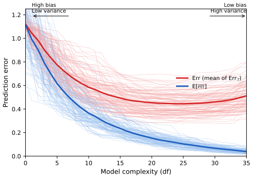
fig_7_1. Reproduces Hastie, Tibshirani and Friedman (2009), Figure 7.1. Download: PDF · SVGFigure 7.1 shows the two facts the chapter is built on. First, the training error is a poor guide: it decreases with complexity, typically to zero, and a model with zero training error has adapted to the noise. Second, the conditional test errors \(\Err_\cT\) of different training sets are spread widely around their mean \(\Err\). We would like to estimate \(\Err_\cT\), the error of the model we actually have; Section 7.12 shows that the methods of this chapter effectively estimate \(\Err\) instead.
Filling the gap 7.1: for nested least-squares fits the training error can only fall p. 221
Let \(V_1\subset V_2\) be the column spaces of two nested designs and \(\hat\by_j=\bH_j\by\) the projections onto them. Then \(\err_2\le\err_1\) for every \(\by\).
Proof
\(\hat\by_2\) is the closest point of \(V_2\) to \(\by\), and \(\hat\by_1\in V_1\subset V_2\) is a candidate, so \(\|\by-\hat\by_2\|^2\le\|\by-\hat\by_1\|^2\). Dividing by \(N\) gives the claim. The same argument works for any family of fits that minimise the training loss over nested sets: best subsets of increasing size, or the lasso and ridge written in constrained form, \(\sum|\beta_j|\le t\) or \(\sum\beta_j^2\le t\), as \(t\) grows (which in penalised form means a decreasing penalty). The test error has no such monotonicity: see Result 7.1. ∎
Two goals must be kept apart. Model selection estimates the performance of competing models (or settings \(\alpha\) of one model) in order to choose; model assessment estimates the prediction error of the finally chosen model. With plenty of data, both are done by splitting it at random into a training set (to fit), a validation set (to compare and choose) and a test set (to assess the chosen model once, at the end); a typical split is 50%, 25%, 25%. The test set must stay locked away until the end, for the reason in the next box.
Filling the gap 7.2: why a test set used for choosing underestimates the error p. 222
Let \(\hat e_1,\dots,\hat e_M\) be unbiased estimates of the true errors \(e_1,\dots,e_M\) of \(M\) models, all computed on the same test set, and let \(\hat m=\argmin_m\hat e_m\). Then \(\E\hat e_{\hat m}\le\min_me_m\le\E e_{\hat m}\): the reported error of the chosen model is biased downward, and so is it relative to the chosen model's own true error.
Proof
For every \(m\), \(\min_j\hat e_j\le\hat e_m\); taking expectations, \(\E\hat e_{\hat m}=\E\min_j\hat e_j\le\E\hat e_m=e_m\). This holds for every \(m\), so \(\E\hat e_{\hat m}\le\min_me_m\). The second inequality holds because \(e_{\hat m}\ge\min_me_m\) for every outcome. Equality in the first requires the minimum to be attained by the same model in almost every sample, which fails as soon as the estimates are noisy and the true errors close; the gap grows with \(M\) and with the noise of the estimates. The same mechanism makes the minimum of a cross-validation curve optimistic (Section 7.11.1). ∎
The methods of this chapter replace the validation step when data are too scarce to split three ways: either analytically (AIC, BIC, MDL, SRM) or by reusing the sample (cross-validation, the bootstrap).
7.3 The Bias–Variance Decomposition
pp. 223–226 Take the additive model \(Y=f(X)+\varepsilon\) with \(\E\varepsilon=0\), \(\Var\varepsilon=\sigma_\varepsilon^2\), \(\varepsilon\) independent of the training data, and squared-error loss.
See also (companion courses): Result 3.8 of Bayesian and Probabilistic Machine Learning and Result 4.12 of Foundations of Deep Learning; in this course, Section 2.9 and Result 2.18.
Result 7.1 (bias–variance decomposition at a point) p. 223, (7.9)
\[ \begin{aligned}\Err(x_0)&=\E\big[(Y-\hf(x_0))^2\given X=x_0\big]\\&=\sigma_\varepsilon^2+\big[\E\hf(x_0)-f(x_0)\big]^2+\E\big[\hf(x_0)-\E\hf(x_0)\big]^2\\&=\sigma_\varepsilon^2+\Bias^2\big(\hf(x_0)\big)+\Var\big(\hf(x_0)\big)\\&=\text{irreducible error}+\text{bias}^2+\text{variance}.\end{aligned} \tag{7.9} \]The expectations are over the training sets (which determine \(\hf\)) and over the new response \(Y\) at \(x_0\).
Proof
Write \[ Y-\hf(x_0)=\varepsilon+\big(f(x_0)-\E\hf(x_0)\big)+\big(\E\hf(x_0)-\hf(x_0)\big), \] a sum of three terms: the new noise, a constant, and a mean-zero random variable that depends on the training set only. Square and take expectations. The three squares give \(\sigma_\varepsilon^2\), the squared bias and the variance. The cross terms vanish: \(\E[\varepsilon\cdot c]=0\); \[ \E[\varepsilon(\E\hf-\hf)]=\E\varepsilon\cdot\E(\E\hf-\hf)=0 \] because the new noise is independent of the training set; and \(\E[c(\E\hf-\hf)]=c\cdot0\). ∎
Result 7.2 (\(k\)-nearest neighbours) p. 223, (7.10)
With the training inputs fixed and \(x_{(1)},\dots,x_{(k)}\) the \(k\) training inputs closest to \(x_0\),
\[ \Err(x_0)=\E\big[(Y-\hf_k(x_0))^2\given X=x_0\big]=\sigma_\varepsilon^2+\Big[f(x_0)-\frac1k\sum_{\ell=1}^kf(x_{(\ell)})\Big]^2+\frac{\sigma_\varepsilon^2}k. \tag{7.10} \]Proof
\(\hf_k(x_0)=\frac1k\sum_{\ell}y_{(\ell)}\) with \(y_{(\ell)}=f(x_{(\ell)})+\varepsilon_{(\ell)}\). With fixed inputs the neighbours are fixed, so \(\E\hf_k(x_0)=\frac1k\sum_\ell f(x_{(\ell)})\) and, the errors being independent with variance \(\sigma_\varepsilon^2\), \(\Var\hf_k(x_0)=\frac1{k^2}\cdot k\sigma_\varepsilon^2=\sigma_\varepsilon^2/k\). Substitute into (7.9). Increasing \(k\) lowers the variance like \(1/k\) and typically raises the bias, since farther neighbours have values \(f(x_{(\ell)})\) less like \(f(x_0)\); \(k\) is inversely related to complexity (and \(N/k\) is the effective number of parameters, Exercise 7.6). ∎
Result 7.3 (least squares with \(p\) parameters) pp. 223–224, (7.11)–(7.12)
Let \(\hf_p(x)=x^\T\hat\beta\) be fitted by least squares on the fixed \(N\times p\) design \(\bX\) of full rank, and \(\bh(x_0)=\bX(\bX^\T\bX)^{-1}x_0\), so that \(\hf_p(x_0)=\bh(x_0)^\T\by\). Then
\[ \Err(x_0)=\E\big[(Y-\hf_p(x_0))^2\given X=x_0\big]=\sigma_\varepsilon^2+\big[f(x_0)-\E\hf_p(x_0)\big]^2+\|\bh(x_0)\|^2\sigma_\varepsilon^2, \tag{7.11} \]and averaged over the training inputs (the in-sample error)
\[ \frac1N\sum_{i=1}^N\Err(x_i)=\sigma_\varepsilon^2+\frac1N\sum_{i=1}^N\big[f(x_i)-\E\hf(x_i)\big]^2+\frac pN\sigma_\varepsilon^2. \tag{7.12} \]Proof
\[ \Var\hf_p(x_0)=\Var(\bh(x_0)^\T\by)=\bh(x_0)^\T(\sigma_\varepsilon^2\bI)\bh(x_0)=\sigma_\varepsilon^2\|\bh(x_0)\|^2, \] and (7.9) gives (7.11). At \(x_0=x_i\), \(\bh(x_i)\) is the \(i\)-th column of the symmetric idempotent hat matrix \(\bH=\bX(\bX^\T\bX)^{-1}\bX^\T\), so \(\|\bh(x_i)\|^2=(\bH^\T\bH)_{ii}=\bH_{ii}\). Hence
\[ \frac1N\sum_i\|\bh(x_i)\|^2=\frac1N\Tr\bH=\frac1N\Tr\big((\bX^\T\bX)^{-1}\bX^\T\bX\big)=\frac pN, \]which is (7.12). The variance at a single point can be far above \(p\sigma^2/N\) (at a high-leverage input) or below it; only the average is fixed. ∎
For ridge regression \(\hf_\alpha(x_0)=x_0^\T(\bX^\T\bX+\alpha\bI)^{-1}\bX^\T\by\) the decomposition (7.11) holds with the weights \(\bh(x_0)=\bX(\bX^\T\bX+\alpha\bI)^{-1}x_0\) (the book prints a transpose in place of the inverse here; see Notes on the book), and with a different bias. For a linear family the bias can be split further. Let
\[ \beta_*=\argmin_\beta\E\big(f(X)-X^\T\beta\big)^2 \tag{7.13} \]be the coefficients of the best linear approximation to \(f\) in the population.
Result 7.4 (model bias and estimation bias) p. 224, (7.14)
For any linear fit \(\hf_\alpha(x_0)=x_0^\T\hat\beta_\alpha\) whose mean \(\E\hat\beta_\alpha\) (over the training responses) is a fixed vector, and \(x_0\) drawn from the input distribution,
\[ \E_{x_0}\big[f(x_0)-\E\hf_\alpha(x_0)\big]^2=\E_{x_0}\big[f(x_0)-x_0^\T\beta_*\big]^2+\E_{x_0}\big[x_0^\T\beta_*-x_0^\T\E\hat\beta_\alpha\big]^2=\Ave[\text{Model Bias}]^2+\Ave[\text{Estimation Bias}]^2. \tag{7.14} \]Proof
Add and subtract \(x_0^\T\beta_*\): \[ f(x_0)-x_0^\T\E\hat\beta_\alpha=\big(f(x_0)-x_0^\T\beta_*\big)+x_0^\T\big(\beta_*-\E\hat\beta_\alpha\big). \] Squaring, the cross term is \[ 2\,\E_{x_0}\big[(f(x_0)-x_0^\T\beta_*)x_0^\T\big](\beta_*-\E\hat\beta_\alpha). \] The minimiser of (7.13) satisfies the normal equations \(\E\big[X(f(X)-X^\T\beta_*)\big]=0\) (differentiate the convex quadratic), so the bracket vanishes and the cross term is zero. Two remarks the book leaves implicit. (i) For least squares on fixed training inputs, \(\E\hat\beta=(\bX^\T\bX)^{-1}\bX^\T\bf\) is the best linear approximation for the empirical distribution of the training inputs; it equals \(\beta_*\), and the estimation bias is exactly zero, when the average in (7.14) is taken over the training inputs (or in the limit \(N\to\infty\)). (ii) For ridge, \(\E\hat\beta_\alpha=(\bX^\T\bX+\alpha\bI)^{-1}\bX^\T\bf\) is shrunk away from that vector, which creates a positive estimation bias in exchange for a smaller variance; the model bias, the first term, does not depend on the fitting method at all and can only be reduced by enlarging the class of models. The identity was confirmed numerically for a ridge fit. ∎
Figure 7.2 of the book draws this geometry schematically (the truth, its projection onto the model space, the spread of the fitted model around that projection, and a shrunken fit closer in total error); it contains nothing computed and is not reproduced. Shrinking or dropping parameters adds estimation bias; it pays when the variance it removes is larger.
7.3.1 Example: Bias–Variance Tradeoff
pp. 226–228 Two simulated problems with \(N=80\) training points and 20 inputs uniform on \([0,1]^{20}\): in the first, \(Y=1\) if \(X_1>1/2\) and 0 otherwise, fitted by \(k\)-nearest neighbours; in the second, \(Y=1\) if \(X_1+\dots+X_{10}>5\) and 0 otherwise, fitted by the best subset linear regression of size \(p\). Each is scored by squared error ("regression") and by the 0–1 loss of the rule \(\hat G=I(\hf>1/2)\) ("classification"). These four scenarios reappear in Sections 7.9.1, 7.10, 7.11.1 and 7.12.
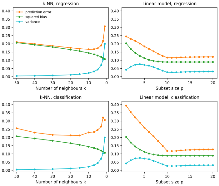
fig_7_3 (the shared simulation is scenario_study). Reproduces Hastie, Tibshirani and Friedman (2009), Figure 7.3. Download: PDF · SVGThe reproduction matches the book closely: for \(k\)-NN regression the error is 0.306 at \(k=1\), smallest (0.166) at \(k=9\) and 0.211 at \(k=50\); for subset regression it is 0.245 at \(p=1\) and levels off at about 0.115 from \(p=10\). Under 0–1 loss the \(k\)-NN error is flat at about 0.21 between \(k=15\) and \(k=30\) although the squared bias keeps rising, and the linear classifier improves much more dramatically from \(p=1\) (0.393) than the regression does. The next result explains why.
Result 7.5 (0–1 loss: bias and variance interact; Exercise 7.2) p. 226, pp. 257–258, (7.62)–(7.63)
Let \(Y\in\{0,1\}\) with \(\Pr(Y=1\given x_0)=f(x_0)\), the Bayes rule \(G(x_0)=I(f(x_0)>\tfrac12)\) with error \[ \Err_B(x_0)=\Pr(Y\ne G(x_0)\given X=x_0)=\min\{f(x_0),1-f(x_0)\}, \] and a rule \(\hat G(x_0)=I(\hf(x_0)>\tfrac12)\) built from a training set independent of the new \(Y\). Then
\[ \Err(x_0)=\Pr\big(Y\ne\hat G(x_0)\given X=x_0\big)=\Err_B(x_0)+|2f(x_0)-1|\,\Pr\big(\hat G(x_0)\ne G(x_0)\given X=x_0\big). \tag{7.62} \]If moreover \(\hf(x_0)\sim N\big(\E\hf(x_0),\Var\hf(x_0)\big)\), then
\[ \Pr\big(\hat G(x_0)\ne G(x_0)\given X=x_0\big)=\Phi\left(\frac{\sgn\big(\tfrac12-f(x_0)\big)\big(\E\hf(x_0)-\tfrac12\big)}{\sqrt{\Var\hf(x_0)}}\right). \tag{7.63} \]Proof, and what it says
Fix \(x_0\) and drop it from the notation. Since the new \(Y\) is independent of \(\hat G\), condition on \(\hat G\): if \(\hat G=1\) the error probability is \(1-f\), if \(\hat G=0\) it is \(f\). Suppose \(f>\tfrac12\), so \(G=1\) and \(\Err_B=1-f\). Then
\[ \Err=(1-f)\Pr(\hat G=1)+f\Pr(\hat G=0)=(1-f)+\big[f-(1-f)\big]\Pr(\hat G=0)=\Err_B+(2f-1)\Pr(\hat G\ne G). \]If \(f\lt \tfrac12\), the same computation with the roles exchanged gives \[ \Err=f+(1-2f)\Pr(\hat G=1)=\Err_B+(1-2f)\Pr(\hat G\ne G). \] Both are (7.62). (If \(f=\tfrac12\) every rule has error \(\tfrac12\) and the second term is 0.)
For (7.63): when \(f>\tfrac12\), \(\hat G\ne G\) means \(\hf\le\tfrac12\), with probability \(\Phi\big((\tfrac12-\E\hf)/\sqrt{\Var\hf}\big)\); here \(\sgn(\tfrac12-f)=-1\), so the argument is \(\sgn(\tfrac12-f)(\E\hf-\tfrac12)/\sqrt{\Var\hf}\). When \(f\lt \tfrac12\), \(\hat G\ne G\) means \(\hf>\tfrac12\), with probability \[ 1-\Phi\big((\tfrac12-\E\hf)/\sqrt{\Var\hf}\big)=\Phi\big((\E\hf-\tfrac12)/\sqrt{\Var\hf}\big), \] and now \(\sgn(\tfrac12-f)=+1\).
Reading it. The bias enters only through which side of \(\tfrac12\) the mean \(\E\hf\) lies on ("boundary bias"): a mean of 0.6 when \(f=0.9\) has squared bias 0.09 but costs nothing as long as the variance is small. Bias and variance combine as a ratio inside \(\Phi\), not as a sum. When \(\E\hf\) is on the correct side the numerator is negative and reducing the variance reduces the error; when it is on the wrong side the numerator is positive and increasing the variance helps, because it makes a correct decision more likely. Averaging over \(x_0\), large squared bias can coexist with near-Bayes error, which is what the bottom-left panel of Figure 7.3 shows. Both identities were confirmed numerically. ∎
The lesson is that a tuning parameter should be chosen by an estimate of the prediction error for the loss that matters, not by a bias–variance calculation done for another loss.
7.4 Optimism of the Training Error Rate
pp. 228–230 Which quantities are fixed and which are random is the whole difficulty here, so the definitions come first.
See also (companion course): Result 1.3 of Foundations of Deep Learning, the same identity for polynomial fits.
Definition 7.2 (extra-sample and in-sample error, optimism) pp. 228–229, (7.15)–(7.20)
With the training set \(\cT\) fixed and \((X^0,Y^0)\sim F\) a new pair, the generalisation error and its average over training sets are
\[ \Err_\cT=\E_{X^0,Y^0}\big[L(Y^0,\hf(X^0))\given\cT\big], \tag{7.15} \] \[ \Err=\E_\cT\E_{X^0,Y^0}\big[L(Y^0,\hf(X^0))\given\cT\big]. \tag{7.16} \]The training error is
\[ \err=\frac1N\sum_{i=1}^NL(y_i,\hf(x_i)). \tag{7.17} \]\(\Err_\cT\) is an extra-sample error: the test inputs need not coincide with the training inputs. The in-sample error keeps the inputs and draws new responses \(Y_i^0\) at each \(x_i\), independent of \(\cT\):
\[ \Err_{\rm in}=\frac1N\sum_{i=1}^N\E_{Y^0}\big[L(Y_i^0,\hf(x_i))\given\cT\big]. \tag{7.18} \]The optimism and the average optimism are
\[ \op\equiv\Err_{\rm in}-\err, \tag{7.19} \] \[ \omega\equiv\E_\by(\op), \tag{7.20} \]where \(\E_\by\) averages over the training responses with the training inputs held fixed.
The training error is usually below \(\Err_\cT\) because the same data fit the model and score it (Exercise 2.9 shows \(\E\err\le\E\Err\) for least squares). The in-sample version isolates the part of the gap caused by the fit adapting to the responses, leaving out the part caused by new inputs falling elsewhere.
Result 7.6 (the optimism is a covariance; Exercise 7.4) p. 229, (7.21)–(7.22)
With the inputs fixed, independent responses, and \(\hy_i=\hf(x_i)\),
\[ \omega=\frac2N\sum_{i=1}^N\Cov(\hy_i,y_i), \tag{7.21} \] \[ \E_\by(\Err_{\rm in})=\E_\by(\err)+\frac2N\sum_{i=1}^N\Cov(\hy_i,y_i), \tag{7.22} \]in each of the following cases: (a) squared-error loss, any fitting rule; (b) 0–1 loss with \(y_i\in\{0,1\}\) and \(\hy_i\in\{0,1\}\) the classification at \(x_i\); (c) deviance loss (7.8) for an exponential family \(\Pr_\theta(y)=\exp\{y\theta-b(\theta)+c(y)\}\), with \(\hy_i\) replaced by the fitted natural parameter \(\hat\theta_i\). For binary data, (c) means the fitted log-odds \(\log\{\hat p_i/(1-\hat p_i)\}\), not the fitted probability \(\hat p_i\) (see Notes on the book).
Proof
(a) Write \(\mu_i=\E y_i\) (\(=f(x_i)\)). The new response \(Y_i^0\) has the same distribution as \(y_i\) and is independent of \(\hy_i\), so
\[ \E_{Y^0}(Y_i^0-\hy_i)^2=\Var(y_i)+(\mu_i-\hy_i)^2. \]For the training term, \[ (y_i-\hy_i)^2=(y_i-\mu_i)^2+(\mu_i-\hy_i)^2+2(y_i-\mu_i)(\mu_i-\hy_i), \] whose expectation is \[ \Var(y_i)+\E(\mu_i-\hy_i)^2-2\E\big[(y_i-\mu_i)\hy_i\big], \] since \(\E(y_i-\mu_i)\mu_i=0\). Subtracting, the first two terms cancel and
\[ \E\big[\E_{Y^0}(Y_i^0-\hy_i)^2-(y_i-\hy_i)^2\big]=2\E\big[(y_i-\mu_i)\hy_i\big]=2\Cov(\hy_i,y_i). \]Average over \(i\). This is the "add and subtract \(f(x_i)\) and \(\E\hf(x_i)\)" computation of Exercise 7.4; no assumption on the fit is needed, and the errors need not be Gaussian or even independent of each other (only \(Y_i^0\) must be independent of the training data).
(b) If \(y,\hy\in\{0,1\}\) then \(I(y\ne\hy)=(y-\hy)^2\), so (b) is (a) applied to binary variables.
(c) The deviance loss is \(-2\{y\hat\theta-b(\hat\theta)+c(y)\}\). The terms \(b(\hat\theta_i)\) are the same in the training and in-sample errors; \(c(Y^0_i)\) and \(c(y_i)\) have equal expectations. What is left is \(-2\hat\theta_i(\E Y_i^0-y_i)=-2\hat\theta_i(\mu_i-y_i)\), whose expectation is \(2\Cov(\hat\theta_i,y_i)\). For binary data \(\theta=\log\{p/(1-p)\}\). An exact enumeration of all \(2^{10}\) outcomes for a smoothed-proportion classifier confirms (b) and (c) and shows that with \(\hat p_i\) in place of the log-odds the covariance formula gives 0.067 instead of the true average optimism 0.306. ∎
So the training error underestimates the in-sample error by an amount that grows with how strongly each \(y_i\) pulls its own fitted value: the harder we fit, the larger \(\Cov(\hy_i,y_i)\).
Result 7.7 (linear fits; Exercise 7.1) pp. 229–230, (7.23)–(7.24)
If \(\hat\by=\bH\by\) is the least-squares fit on \(d\) inputs or basis functions chosen without looking at \(\by\) (\(\bH\) a projection of rank \(d\)), and \(\by=\bf+\be\) with \(\Cov\be=\sigma_\varepsilon^2\bI\), then
\[ \sum_{i=1}^N\Cov(\hy_i,y_i)=d\,\sigma_\varepsilon^2, \tag{7.23} \] \[ \E_\by(\Err_{\rm in})=\E_\by(\err)+2\cdot\frac dN\sigma_\varepsilon^2. \tag{7.24} \]Proof
\[ \Cov(\hat\by,\by)=\Cov(\bH\by,\by)=\bH\Cov(\by)=\sigma_\varepsilon^2\bH, \] so \(\sum_i\Cov(\hy_i,y_i)=\sigma_\varepsilon^2\Tr\bH=d\sigma_\varepsilon^2\), the trace of a projection being its rank. Then (7.22) gives (7.24). One can also see (7.24) directly: \[ \E\,\|\by-\bH\by\|^2=\|(\bI-\bH)\bf\|^2+\sigma_\varepsilon^2(N-d) \] and \[ \E\,\|\by^0-\bH\by\|^2=N\sigma_\varepsilon^2+\|(\bI-\bH)\bf\|^2+d\sigma_\varepsilon^2; \] the difference divided by \(N\) is \(2d\sigma_\varepsilon^2/N\). The optimism grows linearly in \(d\) and shrinks like \(1/N\). Approximate versions hold for other error models such as binary data with deviance loss (Filling the gap 7.3). ∎
Two estimation strategies follow. One estimates the optimism and adds it to \(\err\) (Section 7.5: Cp, AIC, BIC); this works for a special class of fits, those linear in their parameters. The other estimates the extra-sample error directly (cross-validation and the bootstrap, Sections 7.10–7.11), for any loss and any fitting procedure. The in-sample error is rarely of direct interest, since future inputs will not repeat the training inputs, but for comparing models only the relative size matters, and there it is usually adequate.
7.5 Estimates of In-Sample Prediction Error
pp. 230–232 In-sample estimates have the form
\[ \widehat{\Err}_{\rm in}=\err+\hat\omega, \tag{7.25} \]with \(\hat\omega\) an estimate of the average optimism. With \(d\) parameters and squared-error loss, (7.24) gives the Cp statistic
\[ C_p=\err+2\cdot\frac dN\hat\sigma_\varepsilon^2, \tag{7.26} \]with \(\hat\sigma_\varepsilon^2\) estimated from a low-bias model (for instance the residual mean square of the largest model, \(\mathrm{RSS}/(N-d_{\max})\)). For a linear fit with \(d\) fixed in advance and an unbiased \(\hat\sigma_\varepsilon^2\), \(C_p\) is unbiased for \(\E\Err_{\rm in}\), since the penalty is linear in \(\hat\sigma_\varepsilon^2\).
The Akaike information criterion is the corresponding estimate for log-likelihood loss. With \(\Pr_\theta(Y)\) a family of densities containing the true one, \(\hat\theta\) the maximum likelihood estimate and
\[ \loglik=\sum_{i=1}^N\log\Pr_{\hat\theta}(y_i) \tag{7.28} \]the maximised log-likelihood, the relation analogous to (7.24) holds as \(N\to\infty\):
\[ -2\cdot\E\big[\log\Pr_{\hat\theta}(Y)\big]\approx-\frac2N\cdot\E[\loglik]+2\cdot\frac dN. \tag{7.27} \]For logistic regression with the binomial log-likelihood this gives
\[ \AIC=-\frac2N\cdot\loglik+2\cdot\frac dN. \tag{7.29} \]For a family of models \(f_\alpha\) with training errors \(\err(\alpha)\) and \(d(\alpha)\) parameters,
\[ \AIC(\alpha)=\err(\alpha)+2\cdot\frac{d(\alpha)}N\hat\sigma_\varepsilon^2 \tag{7.30} \]estimates the test-error curve, and the chosen model is \(f_{\hat\alpha}\) with \(\hat\alpha=\argmin_\alpha\AIC(\alpha)\).
See also (companion course): Filling the gap 1.3 of Bayesian and Probabilistic Machine Learning (an outline of where the AIC and BIC penalties come from).
Filling the gap 7.3: AIC from the expansion of the log-likelihood p. 230, (7.27)
Setting. \(Y_1,\dots,Y_N\) independent with density \(g\) (for regression, read everything conditionally on fixed inputs; the argument is the same). The model \(\{\Pr_\theta:\theta\in\Theta\subset\R^d\}\) contains \(g=\Pr_{\theta_0}\), \(\theta_0\) interior; \(\theta\mapsto\log\Pr_\theta(y)\) is twice continuously differentiable; the Fisher information per observation \(\mathcal I=-\E\nabla^2\log\Pr_{\theta_0}(Y)\) is positive definite; the MLE \(\hat\theta\) is consistent with \(\sqrt N(\hat\theta-\theta_0)\to N(0,\mathcal I^{-1})\), and the quadratic forms below are uniformly integrable (so that limits of expectations are expectations of limits). Then the expected log-likelihood of a new sample at \(\hat\theta\) and the maximised log-likelihood satisfy
\[ \E\Big[\sum_{i=1}^N\E_{Y^0}\log\Pr_{\hat\theta}(Y_i^0)\Big]=\E[\loglik]-d+o(1), \]which, multiplied by \(-2/N\), is (7.27).
Derivation
Let \(\lambda(\theta)=\E_{Y^0}\log\Pr_\theta(Y^0)\), the expected log-likelihood of one new observation; it is maximised at \(\theta_0\) (Gibbs' inequality: \(\lambda(\theta_0)-\lambda(\theta)=\KL(\Pr_{\theta_0}\|\Pr_\theta)\ge0\)), so \(\nabla\lambda(\theta_0)=0\) and \(-\nabla^2\lambda(\theta_0)=\mathcal I\). Let \(\ell(\theta)=\sum_i\log\Pr_\theta(y_i)\), so \(\loglik=\ell(\hat\theta)\) and \(\nabla\ell(\hat\theta)=0\). Write \(\delta=\hat\theta-\theta_0\).
Step 1 (the new sample). Expand \(\lambda\) about \(\theta_0\): \(N\lambda(\hat\theta)=N\lambda(\theta_0)-\tfrac N2\delta^\T\mathcal I\delta+o_p(1)\), since \(\delta=O_p(N^{-1/2})\).
Step 2 (the training sample). Expand \(\ell\) about its maximiser \(\hat\theta\): \(\ell(\theta_0)=\ell(\hat\theta)-\tfrac12\delta^\T\{-\nabla^2\ell(\tilde\theta)\}\delta\) for some \(\tilde\theta\) between them, and \(-\nabla^2\ell(\tilde\theta)/N\to\mathcal I\) by the law of large numbers and consistency. So \(\ell(\hat\theta)=\ell(\theta_0)+\tfrac N2\delta^\T\mathcal I\delta+o_p(1)\).
Step 3 (subtract and average). \[ \ell(\hat\theta)-N\lambda(\hat\theta)=\{\ell(\theta_0)-N\lambda(\theta_0)\}+N\delta^\T\mathcal I\delta+o_p(1). \] The first brace has expectation exactly 0 (each term of \(\ell(\theta_0)\) has mean \(\lambda(\theta_0)\)). And \(N\delta^\T\mathcal I\delta\to\chi^2_d\) in distribution, because \(\mathcal I^{1/2}\sqrt N\delta\to N(0,\bI_d)\); with uniform integrability its expectation tends to \(d\). Hence \(\E[\ell(\hat\theta)]-\E[N\lambda(\hat\theta)]\to d\).
What it means. Half of the \(d\) comes from the training sample over-rewarding \(\hat\theta\) (Step 2), half from the new sample penalising the distance of \(\hat\theta\) from \(\theta_0\) (Step 1): the same "twice" as in (7.24). For the Gaussian linear model with known \(\sigma^2\), \[ -2\log\Pr_\mu(y)=\log(2\pi\sigma^2)+(y-\mu)^2/\sigma^2, \] so \(-\frac2N\loglik=\log(2\pi\sigma^2)+\err/\sigma^2\) and (7.27) is exactly (7.24) divided by \(\sigma^2\), with no approximation; AIC with known variance and Cp then pick the same model. If the family does not contain \(g\), the same steps with \(\theta_0\) the Kullback–Leibler projection give the correction \(\Tr(\mathcal K\mathcal J^{-1})\) (Takeuchi's information criterion), with \(\mathcal J=-\E\nabla^2\log\Pr_{\theta_0}\) and \(\mathcal K=\Var\nabla\log\Pr_{\theta_0}\); it equals \(d\) when \(\mathcal K=\mathcal J\). A simulation of logistic regression with \(N=400\), \(d=5\) gave an average optimism of the deviance of 0.0248 against \(2d/N=0.025\). ∎
For nonlinear models and adaptive procedures, \(d\) must be replaced by a measure of complexity (Section 7.6). In particular (7.23) fails when the inputs are chosen with the help of \(\by\): choosing the best-fitting \(d\) of \(p\) inputs fits more than \(d\) parameters' worth.
Filling the gap 7.4: a search spends more degrees of freedom than it keeps p. 231
Let the \(q\) inputs be orthonormal columns, \(\bx_j^\T\bx_k=\delta_{jk}\), let \(\by=\be\sim N(0,\sigma^2\bI)\) (no signal), and let the fit use the single best input: \(J=\argmax_j|\bx_j^\T\by|\), \(\hat\by=(\bx_J^\T\by)\bx_J\). Then
\[ \frac1{\sigma^2}\sum_{i=1}^N\Cov(\hy_i,y_i)=\E\Big[\max_{1\le j\le q}Z_j^2\Big],\qquad Z_1,\dots,Z_q\ \text{independent}\ N(0,1), \]which is 1 for \(q=1\) but 1.64 for \(q=2\), 3.46 for \(q=8\) and 4.92 for \(q=20\). One parameter is kept, but the optimism is that of about five.
Proof
Since \(\E\by=0\), \[ \sum_i\Cov(\hy_i,y_i)=\E[\by^\T\hat\by]=\E[(\bx_J^\T\by)^2]=\E[\max_j(\bx_j^\T\by)^2]. \] The \(\bx_j^\T\by\) are jointly Gaussian with covariance \(\sigma^2\bx_j^\T\bx_k=\sigma^2\delta_{jk}\), so they are independent \(N(0,\sigma^2)\); divide by \(\sigma^2\). The numbers are \(\int_0^\infty\{1-F_{\chi^2_1}(t)^q\}\,\d t\), computed by numerical integration. In general the degrees of freedom of a selection rule depend on \(\bf\) (with one dominant input the search almost always picks it and \(\df\approx1\)), which is why no fixed penalty can correct for a search. The optimism demo estimates \(\df\) for forward stepwise on the prostate design: about 16 for an 8-input model chosen from 20 candidates. ∎
Figure 7.4 applies AIC to the phoneme example of Section 5.2.3: a logistic regression on the 256-point log-periodogram, with the coefficient function \(\beta(f)=\sum_{m=1}^Mh_m(f)\theta_m\) expanded in \(M\) natural cubic splines with equally spaced knots, so \(d(M)=M\) (plus an intercept).
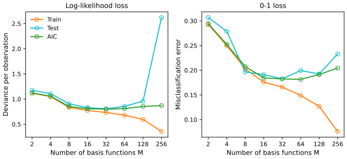
fig_7_4. Reproduces Hastie, Tibshirani and Friedman (2009), Figure 7.4. Download: PDF · SVGThe identity \(\frac2N\sum_i\Cov(\hy_i,y_i)=\frac{2d}N\sigma_\varepsilon^2\) is exact for linear models with additive errors and squared-error loss, and approximate for linear models with log-likelihood loss. For 0–1 loss it has no general justification (Efron, 1986): in Result 7.6(b) the covariance is between \(y_i\) and a thresholded fit, which is not \(d\sigma^2\) for any natural \(\sigma^2\). It is nevertheless often used, and in the right panel it chooses a reasonable model.
7.6 The Effective Number of Parameters
pp. 232–233 Stack the responses into \(\by\) and the fitted values into \(\hat\by\). A linear fitting method is one with
\[ \hat\by=\bS\by, \tag{7.31} \]where the \(N\times N\) matrix \(\bS\) depends on the inputs but not on \(\by\): least squares on a fixed basis, ridge regression, smoothing splines, kernel smoothers, \(k\)-nearest neighbours.
Definition 7.3 (effective degrees of freedom) p. 232, (7.32)–(7.33)
\[ \df(\bS)=\Tr(\bS), \tag{7.32} \]and, for any fitting rule under the additive-error model with \(\Var\varepsilon=\sigma_\varepsilon^2\),
\[ \df(\hat\by)=\frac{\sum_{i=1}^N\Cov(\hy_i,y_i)}{\sigma_\varepsilon^2}. \tag{7.33} \]Result 7.8 (the trace is the right count; Exercise 7.5) p. 233, (7.65)
For a linear smoother \(\hat\by=\bS\by\) and \(\Cov\by=\sigma_\varepsilon^2\bI\),
\[ \sum_{i=1}^N\Cov(\hy_i,y_i)=\Tr(\bS)\,\sigma_\varepsilon^2, \tag{7.65} \]so (7.32) and (7.33) agree, and Cp with \(d=\Tr\bS\) is unbiased for \(\E\Err_{\rm in}\). If \(\bS\) is the orthogonal projection onto a space spanned by \(M\) features, \(\Tr\bS=M\).
Proof and examples
\(\Cov(\hat\by,\by)=\bS\Cov(\by,\by)=\sigma_\varepsilon^2\bS\); sum the diagonal. For a projection, the eigenvalues are \(M\) ones and \(N-M\) zeros. Examples in this course: ridge regression, \(\df(\lambda)=\sum_jd_j^2/(d_j^2+\lambda)\) in terms of the singular values of the centred inputs (Result 3.13, Result 3.20, which also gives the lasso's degrees of freedom); smoothing splines, \(\df_\lambda=\sum_k1/(1+\lambda d_k)\) (Section 5.4.1); local regression (Result 6.7); and \(k\)-nearest neighbours, \(\Tr\bS=N/k\) (Result 2.2, Exercise 7.6). For a nonlinear rule, (7.33) is the definition; Stein's lemma turns it into \(\df=\E\sum_i\partial\hy_i/\partial y_i\) for Gaussian errors and almost differentiable fits, which explains Filling the gap 7.4: a selection rule jumps when the chosen subset changes, and the jumps carry the extra covariance. The identity (7.65) was confirmed by simulation for ridge regression. ∎
For models such as neural networks fitted by minimising \(R(w)+\alpha\sum_mw_m^2\) (weight decay), the effective number of parameters is
\[ \df(\alpha)=\sum_{m=1}^M\frac{\theta_m}{\theta_m+\alpha}, \tag{7.34} \]with \(\theta_m\) the eigenvalues of the Hessian \(\partial^2R(w)/\partial w\partial w^\T\) at the solution (Bishop, 1995). The derivation fixes a convention that the book leaves implicit.
See also (companion courses): Result 3.20 of Bayesian and Probabilistic Machine Learning (\(\gamma\), the number of well-determined parameters) and Result 9.4 of Foundations of Deep Learning.
Filling the gap 7.5: where (7.34) comes from, and the factor 2 p. 233
Suppose \(R(w)=\sum_i(y_i-g(x_i;w))^2/c\) for some constant \(c>0\), and the fit minimises \(R(w)+\tfrac\alpha2\sum_mw_m^2\). Linearise the model about the solution, \(g(x_i;w)\approx g_i+\bm j_i^\T(w-\hat w)\), so that locally the fit is ridge regression in the Jacobian rows \(\bm j_i^\T\). Then the Hessian is \(\bm\Theta=\partial^2R/\partial w\partial w^\T=\frac2c\mathbf J^\T\mathbf J\) and the smoother matrix of the linearised problem is \(\bS=\mathbf J(\mathbf J^\T\mathbf J+\tfrac{c\alpha}2\bI)^{-1}\mathbf J^\T\), whose trace is \(\sum_m\theta_m/(\theta_m+\alpha)\) with \(\theta_m\) the eigenvalues of \(\bm\Theta\).
Derivation
The stationarity condition of \(R(w)+\tfrac\alpha2\|w\|^2\) for the linearised model is \(\tfrac2c\mathbf J^\T(\mathbf J w-\tilde\by)=-\alpha w\) for a working response \(\tilde\by\), i.e. \(w=(\mathbf J^\T\mathbf J+\tfrac{c\alpha}2\bI)^{-1}\mathbf J^\T\tilde\by\), and the fitted values are \(\mathbf J w=\bS\tilde\by\). With the eigendecomposition \(\mathbf J^\T\mathbf J=\mathbf V\diag(\nu_m)\mathbf V^\T\), \(\Tr\bS=\sum_m\nu_m/(\nu_m+c\alpha/2)\). Since \(\theta_m=2\nu_m/c\), \(\nu_m/(\nu_m+c\alpha/2)=\theta_m/(\theta_m+\alpha)\). So (7.34) holds when the penalty is \(\tfrac\alpha2\sum w_m^2\), Bishop's convention. With the penalty \(\alpha\sum w_m^2\) written in the book, the same steps give \(\sum_m\theta_m/(\theta_m+2\alpha)\) (Notes on the book). Example: for ridge regression \(R=\|\by-\bX w\|^2\) (\(c=1\)) and penalty \(\alpha\|w\|^2\), the trace of the smoother is \(\sum d_j^2/(d_j^2+\alpha)=\sum\theta_j/(\theta_j+2\alpha)\) with \(\theta_j=2d_j^2\); numerically, 3.748 against 3.870 for the formula as printed. The approximation itself treats the network as linear in its weights near the solution, so it is only as good as that local quadratic picture. ∎
7.7 The Bayesian Approach and BIC
pp. 233–235 The Bayesian information criterion applies, like AIC, when fitting maximises a log-likelihood:
\[ \BIC=-2\cdot\loglik+(\log N)\cdot d. \tag{7.35} \](Half of it is the Schwarz criterion; Schwarz, 1978.) For the Gaussian model with known \(\sigma_\varepsilon^2\), \(-2\loglik\) equals \(\sum_i(y_i-\hf(x_i))^2/\sigma_\varepsilon^2=N\err/\sigma_\varepsilon^2\) up to a constant, so
\[ \BIC=\frac N{\sigma_\varepsilon^2}\Big[\err+(\log N)\cdot\frac dN\sigma_\varepsilon^2\Big]. \tag{7.36} \]BIC is AIC (Cp) with the factor 2 replaced by \(\log N\); since \(\log N>2\) once \(N>e^2\approx7.4\), BIC penalises complexity more and prefers smaller models. With the multinomial log-likelihood the same relation holds for classification with the deviance; the misclassification rate has no likelihood behind it and does not fit the BIC framework. The motivation, though, is quite different from AIC's. Given candidate models \(\cM_1,\dots,\cM_M\) with parameters \(\theta_m\), priors \(\Pr(\theta_m\given\cM_m)\) and data \(\mathbf Z=\{x_i,y_i\}_1^N\), the posterior probability of a model is
\[ \Pr(\cM_m\given\mathbf Z)\propto\Pr(\cM_m)\cdot\Pr(\mathbf Z\given\cM_m)\propto\Pr(\cM_m)\cdot\int\Pr(\mathbf Z\given\theta_m,\cM_m)\Pr(\theta_m\given\cM_m)\,\d\theta_m. \tag{7.37} \]Two models are compared by the posterior odds
\[ \frac{\Pr(\cM_m\given\mathbf Z)}{\Pr(\cM_\ell\given\mathbf Z)}=\frac{\Pr(\cM_m)}{\Pr(\cM_\ell)}\cdot\frac{\Pr(\mathbf Z\given\cM_m)}{\Pr(\mathbf Z\given\cM_\ell)}, \tag{7.38} \]and the data enter only through the Bayes factor
\[ \mathrm{BF}(\mathbf Z)=\frac{\Pr(\mathbf Z\given\cM_m)}{\Pr(\mathbf Z\given\cM_\ell)}. \tag{7.39} \]See also (companion course): Section 3.4 (Bayesian model comparison) and Results 4.18–4.19 (the Laplace approximation of the evidence and BIC) of Bayesian and Probabilistic Machine Learning, where the same derivation is done in full.
Result 7.9 (BIC is a Laplace approximation of the log evidence) p. 234, (7.40)
Suppose the log-likelihood \(\ell(\theta)=\log\Pr(\mathbf Z\given\theta,\cM_m)\) of a \(d_m\)-parameter model has a unique interior maximiser \(\hat\theta_m\), with \(-\nabla^2\ell(\hat\theta_m)=N\hat{\mathcal J}\) where \(\hat{\mathcal J}\) converges to a positive definite matrix; the prior density is continuous and positive at the limit of \(\hat\theta_m\); and the likelihood away from \(\hat\theta_m\) is negligible compared with its peak (the usual conditions of Laplace's method). Then
\[ \log\Pr(\mathbf Z\given\cM_m)=\log\Pr(\mathbf Z\given\hat\theta_m,\cM_m)-\frac{d_m}2\cdot\log N+O(1). \tag{7.40} \]So with the loss \(-2\log\Pr(\mathbf Z\given\hat\theta_m,\cM_m)\), \(-2\log\Pr(\mathbf Z\given\cM_m)=\BIC_m+O(1)\), and with equal prior model probabilities the model of smallest BIC has (approximately) the largest posterior probability.
Derivation by Laplace's method
Write the evidence as \(\int e^{\ell(\theta)}\pi(\theta)\,\d\theta\). Near \(\hat\theta\) a second-order Taylor expansion with \(\nabla\ell(\hat\theta)=0\) gives \[ \ell(\theta)=\ell(\hat\theta)-\tfrac N2(\theta-\hat\theta)^\T\hat{\mathcal J}(\theta-\hat\theta)+r(\theta), \] where \(r\) is of third order in \(\theta-\hat\theta\) times \(N\). Substitute \(u=\sqrt N(\theta-\hat\theta)\), \(\d\theta=N^{-d/2}\d u\):
\[ \int e^{\ell(\theta)}\pi(\theta)\,\d\theta=e^{\ell(\hat\theta)}N^{-d/2}\int e^{-\frac12u^\T\hat{\mathcal J}u+r(\hat\theta+u/\sqrt N)}\,\pi(\hat\theta+u/\sqrt N)\,\d u. \]For fixed \(u\), \(r(\hat\theta+u/\sqrt N)=O(N^{-1/2})\to0\) and \(\pi(\hat\theta+u/\sqrt N)\to\pi(\hat\theta)\); the conditions above make the contribution of large \(u\) negligible, so the last integral tends to \[ \pi(\hat\theta)\int e^{-\frac12u^\T\hat{\mathcal J}u}\d u=\pi(\hat\theta)(2\pi)^{d/2}|\hat{\mathcal J}|^{-1/2}. \] Taking logarithms,
\[ \log\Pr(\mathbf Z\given\cM)=\ell(\hat\theta)-\frac d2\log N+\Big[\log\pi(\hat\theta)+\frac d2\log(2\pi)-\frac12\log|\hat{\mathcal J}|\Big]+o(1). \]The bracket stays bounded as \(N\) grows; dropping it is the "other simplification" that turns Laplace's approximation into (7.40). It is also why BIC can be poor for moderate \(N\): the dropped term depends on the prior and on the information matrix, and can differ substantially between models. For the Gaussian linear model with a Gaussian prior and known variance, Laplace's formula (with the posterior mode and the posterior precision) is exact; the computation of the difference \(\log\Pr(\mathbf Z\given\cM)-[\ell(\hat\theta)-\frac d2\log N]\) gave \(-2.19,-2.18,-2.24,-2.24\) at \(N=10^2,10^3,10^4,10^5\): bounded, as claimed. ∎
Computing \(\BIC_m\) for each model gives approximate posterior model probabilities,
\[ \Pr(\cM_m\given\mathbf Z)\approx\frac{e^{-\frac12\BIC_m}}{\sum_{\ell=1}^Me^{-\frac12\BIC_\ell}}, \tag{7.41} \]which assess the relative merits of the models as well as picking the best one. A difference of 2 in BIC is a factor \(e\approx2.7\) in the odds, a difference of 6 a factor of 20.
Result 7.10 (BIC is consistent, AIC is not) p. 235
Compare two nested Gaussian linear models with known \(\sigma^2\): \(\cM_0\) with \(d_0\) parameters inside \(\cM_1\) with \(d_1=d_0+k\), on designs with \(\bX^\T\bX/N\) converging to a positive definite matrix. (a) If \(\cM_0\) is true, AIC chooses \(\cM_1\) with probability \(\Pr(\chi^2_k>2k)\) for every \(N\) (0.157 for \(k=1\)), while BIC chooses it with probability \(\Pr(\chi^2_k>k\log N)\to0\). (b) If \(\cM_0\) is false and \(\cM_1\) true, both choose \(\cM_1\) with probability tending to 1.
Proof
The criteria differ by \(\Delta=\frac{\mathrm{RSS}_0-\mathrm{RSS}_1}{\sigma^2}-c_Nk\) with \(c_N=2\) (AIC) or \(\log N\) (BIC); \(\cM_1\) is chosen when \(\Delta>0\). \(\mathrm{RSS}_0-\mathrm{RSS}_1=\|(\bH_1-\bH_0)\by\|^2\), and \(\bH_1-\bH_0\) is the projection onto a \(k\)-dimensional space. (a) Under \(\cM_0\), \((\bH_1-\bH_0)\bf=0\), so \((\mathrm{RSS}_0-\mathrm{RSS}_1)/\sigma^2\sim\chi^2_k\) exactly, and the two probabilities follow. (b) Under \(\cM_1\) with \(\cM_0\) false, \(\|(\bH_1-\bH_0)\bf\|^2=N\delta_N\) with \(\delta_N\to\delta>0\) by the design assumption, so the statistic is a noncentral \(\chi^2_k\) with noncentrality \(N\delta_N/\sigma^2\): it grows linearly in \(N\), faster than \(k\log N\), and both criteria pick \(\cM_1\) with probability tending to 1. Hence BIC selects the true model among finitely many nested candidates with probability tending to 1; AIC keeps a fixed probability of overfitting. For finite \(N\) the heavier penalty is a liability when small effects matter: the optimism demo shows BIC choosing models with two inputs far more often than Cp. ∎
7.8 Minimum Description Length
pp. 235–237 Minimum description length (Rissanen, 1983) arrives at a criterion of the same form as BIC from data compression: a model is a way of encoding the data, and the best model gives the shortest code. Suppose messages \(z_1,\dots,z_m\) are encoded in an alphabet of \(A\) symbols, for example binary (\(A=2\)):
| Message | \(z_1\) | \(z_2\) | \(z_3\) | \(z_4\) | \((7.42)\) |
|---|---|---|---|---|---|
| Code | 0 | 10 | 110 | 111 |
This is an instantaneous prefix code: no codeword is the beginning of another, so the receiver knows when a message ends. Frequent messages should get short codewords.
See also (companion course): Section 1.6 (information theory) and Result 1.22 (Gibbs' inequality) of Bayesian and Probabilistic Machine Learning.
Result 7.11 (Kraft's inequality and Shannon's bound) p. 236, (7.43)
A prefix code with codeword lengths \(l_i\) over an alphabet of size \(A\) satisfies \(\sum_iA^{-l_i}\le1\). If message \(z_i\) is sent with probability \(\Pr(z_i)\), the average length satisfies
\[ \E(\text{length})\ge-\sum_i\Pr(z_i)\log_A\Pr(z_i), \tag{7.43} \]with equality if and only if \(\Pr(z_i)=A^{-l_i}\) for all \(i\). Conversely, lengths \(l_i=\lceil-\log_A\Pr(z_i)\rceil\) satisfy Kraft's inequality, so a prefix code with average length below the entropy plus one exists.
Proof
Kraft. Let \(L=\max l_i\). Codewords are nodes of the complete \(A\)-ary tree of depth \(L\); a codeword of length \(l_i\) has \(A^{L-l_i}\) descendants at depth \(L\), and by the prefix property these sets are disjoint. There are \(A^L\) leaves, so \(\sum_iA^{L-l_i}\le A^L\).
Lower bound. Put \(p_i=\Pr(z_i)\), \(q_i=A^{-l_i}/s\) with \(s=\sum_jA^{-l_j}\le1\). Then
\[ \sum_ip_il_i+\sum_ip_i\log_Ap_i=\sum_ip_i\log_A\frac{p_i}{A^{-l_i}}=\sum_ip_i\log_A\frac{p_i}{q_i}-\log_As\ge0, \]because the first sum is a Kullback–Leibler divergence (nonnegative by Gibbs' inequality, Jensen applied to the concave logarithm) and \(-\log_As\ge0\). Equality needs \(p=q\) and \(s=1\), i.e. \(p_i=A^{-l_i}\).
Achievability. \(l_i\ge-\log_Ap_i\) gives \(\sum_iA^{-l_i}\le\sum_ip_i=1\), and Kraft's inequality is also sufficient for a prefix code to exist (assign codewords in order of increasing length, each time taking the first free node). Since \(l_i\lt -\log_Ap_i+1\), the average length is below the entropy plus one; Huffman's algorithm finds the shortest possible average length. For (7.42) with probabilities \(\tfrac12,\tfrac14,\tfrac18,\tfrac18\), \(p_i=2^{-l_i}\) exactly and the average length 1.75 bits equals the entropy. ∎
So transmitting a random variable with density \(\Pr(z)\) takes about \(-\log_2\Pr(z)\) bits; switching to natural logarithms only changes the unit. (For a continuous \(z\) sent to precision \(\delta z\), the probability of the cell is about \(\Pr(z)\delta z\), and \[ -\log\{\Pr(z)\delta z\}=-\log\Pr(z)-\log\delta z: \] the constant \(-\log\delta z\) can be ignored when comparing models.) For model selection, with a model \(\cM\), parameters \(\theta\) and data \(\mathbf Z=(\bX,\by)\) where the receiver already knows the inputs, the message length for the outputs is
\[ \text{length}=-\log\Pr(\by\given\theta,\cM,\bX)-\log\Pr(\theta\given\cM): \tag{7.44} \]the cost of the discrepancies between data and model plus the cost of the parameters. For a single \(y\sim N(\theta,\sigma^2)\) with prior \(\theta\sim N(0,1)\) and no inputs,
\[ \text{length}=\text{constant}+\log\sigma+\frac{(y-\theta)^2}{2\sigma^2}+\frac{\theta^2}2, \tag{7.45} \]where the constant is \(\log(2\pi)\). (The book prints \((y-\theta)^2/\sigma^2\); the Gaussian log density has \(2\sigma^2\) in the denominator, see Notes on the book.) A smaller \(\sigma\) shortens the average message, since \(y\) is then more concentrated around \(\theta\). Minimising (7.44) is maximising \(\Pr(\by\given\theta)\Pr(\theta)\), the posterior density: MDL is MAP estimation, and since BIC approximates the log posterior probability of a model, BIC can be read as (approximate) model choice by minimum description length.
Filling the gap 7.6: why a parameter costs \(\tfrac12\log N\) pp. 236–237
In the two-part code the parameter must itself be sent, to some precision \(\delta\) per coordinate. Under the conditions of Result 7.9, the precision that minimises the total length is of order \(N^{-1/2}\), and the minimal total length is \(-\ell(\hat\theta)+\frac d2\log N+O(1)\): exactly half the BIC.
Derivation
Send \(\tilde\theta\), the MLE rounded to a grid of mesh \(\delta\). Its cost is about \[ -\log\{\pi(\tilde\theta)\delta^d\}=-\log\pi(\tilde\theta)-d\log\delta \] (the probability of its grid cell under the prior). Sending the data with \(\tilde\theta\) instead of \(\hat\theta\) costs \[ -\ell(\tilde\theta)\approx-\ell(\hat\theta)+\tfrac N2(\tilde\theta-\hat\theta)^\T\hat{\mathcal J}(\tilde\theta-\hat\theta), \] and the rounding error has components of order \(\delta\), so the extra term is about \(cN\delta^2\) for a constant \(c>0\). The total \(-\ell(\hat\theta)+cN\delta^2-d\log\delta+O(1)\) is minimised at \(\delta^2=d/(2cN)\), where \(-d\log\delta=\frac d2\log N+O(1)\) and \(cN\delta^2=d/2\). Coarser precision wastes bits on the data, finer on the parameters; the balance is the estimation precision \(N^{-1/2}\), and it puts \(\frac d2\log N\) on the parameters. ∎
The MDL view as stated selects the model of highest posterior probability; many Bayesians would rather average over the posterior (or sample from it) than select a single model.
7.9 Vapnik–Chervonenkis Dimension
pp. 237–239 In-sample estimates need the number of parameters, and the effective number of Section 7.6 does not cover every nonlinear method. The Vapnik–Chervonenkis theory measures the complexity of a class of functions \(\{f(x,\alpha)\}\) in a way that does not count parameters, and bounds the optimism uniformly over the class. Parameter counting can mislead in both directions: the one-parameter class \(I(\sin\alpha x>0)\), \(x\in\R\), is at least as rich as the two-parameter class of half-lines \(I(\alpha_0+\alpha_1x>0)\) (Figure 7.5).
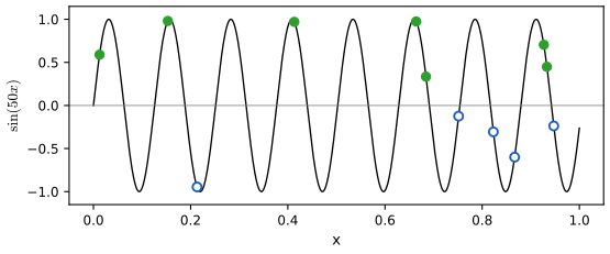
fig_7_5. Reproduces Hastie, Tibshirani and Friedman (2009), Figure 7.5. Download: PDF · SVGDefinition 7.4 (shattering and VC dimension) p. 238
A set of points is shattered by a class of indicator functions if every one of the \(2^n\) assignments of binary labels to the \(n\) points is realised exactly by some member of the class. The VC dimension of \(\{f(x,\alpha)\}\) is the largest \(n\) for which some configuration of \(n\) points is shattered (infinite if there is no largest). For real-valued functions \(\{g(x,\alpha)\}\), the VC dimension is that of the indicator class \(\{I(g(x,\alpha)-\beta>0)\}\), with \(\beta\) ranging over the values of \(g\).
Result 7.12 (half-spaces in \(\R^p\) have VC dimension \(p+1\)) p. 238, Figure 7.6
The class \[ \{I(\alpha_0+\alpha^\T x>0):\alpha_0\in\R,\alpha\in\R^p\} \] shatters some set of \(p+1\) points and no set of \(p+2\) points. In the plane, lines shatter three points in general position but no four points.
Proof
\(p+1\) points are shattered. Take \(0,\mathbf e_1,\dots,\mathbf e_p\) (the origin and the unit vectors) with any labels \(y_0,\dots,y_p\in\{0,1\}\). Put \(\alpha_0=y_0-\tfrac12\) and \(\alpha_j=y_j-\tfrac12-\alpha_0\). Then \(\alpha_0+\alpha^\T0=y_0-\tfrac12\) and \(\alpha_0+\alpha^\T\mathbf e_j=y_j-\tfrac12\), positive exactly when the label is 1.
No \(p+2\) points are shattered (Radon's theorem). Given \(x_1,\dots,x_{p+2}\in\R^p\), the \(p+2\) vectors \((x_i,1)\in\R^{p+1}\) are linearly dependent: \(\sum_ic_i(x_i,1)=0\) with \(c\ne0\). The last coordinate gives \(\sum_ic_i=0\), so both \(P=\{i:c_i>0\}\) and \(Q=\{i:c_i\le0\}\) are nonempty; with \(s=\sum_{i\in P}c_i>0\), the point \(z=\sum_{i\in P}\frac{c_i}sx_i=\sum_{i\in Q}\frac{-c_i}sx_i\) is a convex combination of the points of \(P\) and also of those of \(Q\). Label \(P\) with 1 and \(Q\) with 0. A half-space realising it would have \(\alpha_0+\alpha^\T x_i>0\) on \(P\), hence \(\alpha_0+\alpha^\T z>0\) (convex combination), and \(\alpha_0+\alpha^\T x_i\le0\) on \(Q\), hence \(\alpha_0+\alpha^\T z\le0\): impossible. In the plane (\(p=2\)) the XOR configuration of Figure 7.6 is the case \(P\)=one diagonal, \(Q\)=the other. A linear-programming check of all labellings confirmed both statements, and found an unrealisable labelling for each of 100 random four-point sets. ∎
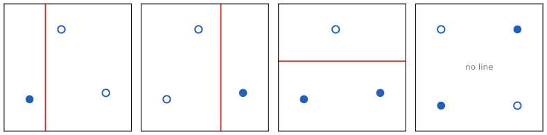
fig_7_6. Reproduces Hastie, Tibshirani and Friedman (2009), Figure 7.6. Download: PDF · SVGA linear indicator in \(p\) dimensions thus has VC dimension \(p+1\), its number of free parameters; the family \(I(\sin\alpha x>0)\) has infinite VC dimension (Exercise 7.8). With \(h\) the VC dimension of the class fitted to \(N\) points, the following holds with probability at least \(1-\eta\) over training sets, simultaneously for all members of the class:
\[ \Err_\cT\le\err+\frac\epsilon2\Big(1+\sqrt{1+\frac{4\cdot\err}\epsilon}\Big)\quad\text{(binary classification)},\qquad \Err_\cT\le\frac{\err}{(1-c\sqrt\epsilon)_+}\quad\text{(regression)}, \] \[ \text{where}\quad\epsilon=a_1\frac{h\,[\log(a_2N/h)+1]-\log(\eta/4)}N,\quad 0\lt a_1\le4,\ 0\lt a_2\le2. \tag{7.46} \]These bounds are taken from Cherkassky and Mulier (2007). The classification bound with \(a_1=4\), \(a_2=2\) is Vapnik's worst case and is a theorem (next box); smaller constants and the regression bound, with \(c=1\) and \(a_1=a_2=1\) recommended for practice, are practical versions whose validity needs further assumptions on the loss (bounded or light-tailed). \((u)_+=\max(u,0)\), and the regression bound is infinite when \(c\sqrt\epsilon\ge1\). A tuning-free alternative for regression is
\[ \Err_\cT\le\err\Big(1-\sqrt{\rho-\rho\log\rho+\frac{\log N}{2N}}\Big)_+^{-1},\qquad\rho=\frac hN. \tag{7.47} \]Filling the gap 7.7: where the classification bound (7.46) comes from p. 239
Vapnik's relative deviation inequality (Vapnik, 1998), stated without proof: for a class of indicator losses \(Q(z,\alpha)\in\{0,1\}\) with risks \(R(\alpha)=\E Q\) and empirical risks \(R_{\rm emp}(\alpha)\) on \(N\) independent observations,
\[ \Pr\Big\{\sup_\alpha\frac{R(\alpha)-R_{\rm emp}(\alpha)}{\sqrt{R(\alpha)}}>\varepsilon\Big\}\lt 4\,\Pi(2N)\,e^{-N\varepsilon^2/4}, \]where the growth function \(\Pi(n)\) is the largest number of distinct labellings the class produces on \(n\) points. Sauer's lemma bounds it by the VC dimension \(h\): \(\Pi(n)\le\sum_{i=0}^h\binom ni\le(en/h)^h\) for \(n\ge h\). Together they give (7.46) with \(a_1=4\), \(a_2=2\).
Proof of Sauer's lemma and of the bound
Sauer's lemma. Let \(\mathcal F\) be the set of labellings (subsets) the class induces on \(n\) points, with VC dimension at most \(h\); write \(\Phi_h(n)=\sum_{i\le h}\binom ni\). Induction on \(n\) (trivial for \(n=0\) or \(h=0\)). Remove one point \(x\): let \(\mathcal F_1\) be the restrictions of the sets in \(\mathcal F\) to the other \(n-1\) points, and \(\mathcal F_2\) the subsets \(A\) of the other points with both \(A\) and \(A\cup\{x\}\) in \(\mathcal F\). Each element of \(\mathcal F_1\) comes from one or two sets of \(\mathcal F\), two exactly for those in \(\mathcal F_2\), so \(|\mathcal F|=|\mathcal F_1|+|\mathcal F_2|\). \(\mathcal F_1\) has VC dimension at most \(h\); if \(\mathcal F_2\) shattered a set \(T\), \(\mathcal F\) would shatter \(T\cup\{x\}\), so \(\mathcal F_2\) has VC dimension at most \(h-1\). By induction \[ |\mathcal F|\le\Phi_h(n-1)+\Phi_{h-1}(n-1)=\Phi_h(n) \] (Pascal's rule). For the closed form, with \(t=h/n\le1\): \[ \Phi_h(n)\,t^h\le\sum_{i\le h}\binom nit^i\le(1+t)^n\le e^{tn}=e^h, \] so \(\Phi_h(n)\le(en/h)^h\).
The bound. Set the right side of Vapnik's inequality equal to \(\eta\) and use Sauer: \[ \varepsilon^2=\frac4N\{\log\Pi(2N)-\log(\eta/4)\}\le4\,\frac{h[\log(2N/h)+1]-\log(\eta/4)}N, \] which is \(\epsilon\) of (7.46) with \(a_1=4\), \(a_2=2\). With probability at least \(1-\eta\), every \(\alpha\) has \(R-R_{\rm emp}\le\sqrt{\epsilon R}\). Put \(r=\sqrt R\): \(r^2-\sqrt\epsilon\,r-R_{\rm emp}\le0\), so \(r\le\tfrac12\big(\sqrt\epsilon+\sqrt{\epsilon+4R_{\rm emp}}\big)\); squaring,
\[ R\le R_{\rm emp}+\frac\epsilon2+\frac{\sqrt\epsilon\sqrt{\epsilon+4R_{\rm emp}}}2=R_{\rm emp}+\frac\epsilon2\Big(1+\sqrt{1+\frac{4R_{\rm emp}}\epsilon}\Big), \]the classification bound of (7.46) with \(R=\Err_\cT\), \(R_{\rm emp}=\err\). Because it holds for all members of the class at once, it remains valid for the member chosen by minimising \(\err\), unlike (7.24), which is for a fixed model. The counting bound and the solved quadratic were checked numerically. ∎
The bounds grow with \(h\) and shrink with \(N\), in qualitative agreement with the AIC correction \(d/N\). Structural risk minimisation (SRM) fits a nested sequence of classes of VC dimensions \(h_1\lt h_2\lt \cdots\) and chooses the one with the smallest upper bound. Such bounds are usually very loose, which matters less for selection, where only relative sizes count; the practical obstacle is computing \(h\), for which often only a crude upper bound is available. The support vector classifier (Section 12.2 of the book) is a case where SRM can be carried out.
7.9.1 Example (Continued)
pp. 239–241 Figure 7.7 uses AIC, BIC and SRM to choose \(k\) or \(p\) in the four scenarios of Figure 7.3. For each of 100 training sets the criterion picks \(\hat\alpha\); its test error \(\Err_\cT(\hat\alpha)\) on 10,000 test points is compared with the best and worst possible choices for that training set, through
\[ 100\times\frac{\Err_\cT(\hat\alpha)-\min_\alpha\Err_\cT(\alpha)}{\max_\alpha\Err_\cT(\alpha)-\min_\alpha\Err_\cT(\alpha)}. \]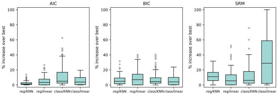
fig_7_7, selection_study. Reproduces Hastie, Tibshirani and Friedman (2009), Figure 7.7. Download: PDF · SVGFor linear regression the complexity is the number of inputs, which undercharges for the search over subsets (Filling the gap 7.4); the same count is used as the VC dimension of the linear classifier. For \(k\)-NN, \(N/k\) is the exact effective degrees of freedom under an additive-error model (Exercise 7.6), whether or not it is the VC dimension. As in the book, AIC works well in all four scenarios despite the lack of theory for 0–1 loss, BIC nearly as well, and SRM is mixed (here, poor for class/linear). The book reports SRM results as sensitive to the constants, with \(a_1=a_2=1\) the most favourable and (7.47) giving almost the same; I did not explore other constants.
7.10 Cross-Validation
p. 241 Cross-validation is probably the simplest and most widely used estimate of prediction error. It estimates the extra-sample error \(\Err=\E[L(Y,\hf(X))]\) directly; one might hope that it estimates the conditional error \(\Err_\cT\) of the training set at hand, but Section 7.12 shows that it does well only for \(\Err\).
7.10.1 K-Fold Cross-Validation
pp. 241–245 Split the data into \(K\) roughly equal parts. For the \(k\)-th part, fit the model to the other \(K-1\) parts and compute its error in predicting the \(k\)-th; do this for \(k=1,\dots,K\) and combine. With \(\kappa:\{1,\dots,N\}\to\{1,\dots,K\}\) the random assignment of observations to parts and \(\hf^{-k}\) the fit with the \(k\)-th part removed,
\[ \CV(\hf)=\frac1N\sum_{i=1}^NL\big(y_i,\hf^{-\kappa(i)}(x_i)\big). \tag{7.48} \]\(K=5\) or 10 are typical; \(K=N\) is leave-one-out cross-validation (\(\kappa(i)=i\)). For a family of models \(f(x,\alpha)\),
\[ \CV(\hf,\alpha)=\frac1N\sum_{i=1}^NL\big(y_i,\hf^{-\kappa(i)}(x_i,\alpha)\big) \tag{7.49} \]estimates the test-error curve; we choose \(\hat\alpha\) to minimise it and refit \(f(x,\hat\alpha)\) to all the data.
See also (companion courses): Section 1.2.6 of Foundations of Deep Learning and Section 1.3 of Bayesian and Probabilistic Machine Learning (validation sets and cross-validation).
Which \(K\)? Each fold's fit uses \(N(K-1)/K\) observations, so CV estimates the error of a rule trained on fewer points than we have. Whether that matters depends on the learning curve, the error as a function of the training-set size: if it is still falling steeply at \(N\), CV is biased upward. Leave-one-out has almost no such bias. The book adds that it can have high variance, because the \(N\) training sets are so alike, and is expensive; 5- or 10-fold CV is the usual compromise (Breiman and Spector, 1992; Kohavi, 1995). The variance claim is not universal: in the simulation of Figure 7.14 the standard deviation over training sets at \(p=10\) is 0.0216 for leave-one-out and 0.0222 for 10-fold CV. The book's Figure 7.8 is a hand-drawn learning curve; Figure 7.S1 computes one.
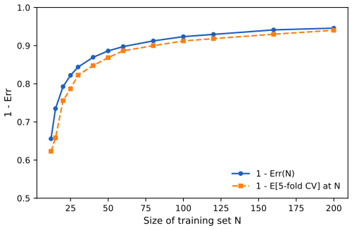
fig_7_s1. Download: PDF · SVG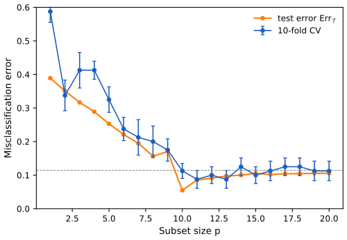
fig_7_9. Reproduces Hastie, Tibshirani and Friedman (2009), Figure 7.9. Download: PDF · SVGGeneralised cross-validation approximates leave-one-out for linear fits under squared error. With
\[ \hat\by=\bS\by, \tag{7.50} \]many linear fitting methods satisfy
\[ \frac1N\sum_{i=1}^N\big[y_i-\hf^{-i}(x_i)\big]^2=\frac1N\sum_{i=1}^N\Big[\frac{y_i-\hf(x_i)}{1-S_{ii}}\Big]^2, \tag{7.51} \]and GCV replaces each \(S_{ii}\) by their average:
\[ \GCV(\hf)=\frac1N\sum_{i=1}^N\Big[\frac{y_i-\hf(x_i)}{1-\Tr(\bS)/N}\Big]^2. \tag{7.52} \]Result 7.13 (leave-one-out from one fit; Exercise 7.3) pp. 244, 258, (7.51), (7.64)
Call a linear smoother self-stable if the leave-one-out fit at \(x_i\) equals the full-data fit applied to \(\by\) with \(y_i\) replaced by that leave-one-out value. Then
\[ y_i-\hf^{-i}(x_i)=\frac{y_i-\hf(x_i)}{1-S_{ii}}. \tag{7.64} \]Every penalised least-squares fit \[ \hf=\argmin_{g\in\mathcal G}\{\sum_j(y_j-g(x_j))^2+J(g)\} \] over a fixed class \(\mathcal G\) is self-stable: least squares on any basis (\(J=0\)), ridge, cubic smoothing splines, penalised splines; so is any weighted least-squares local fit with weights that do not depend on which points are present (local polynomial regression with a fixed metric window). If moreover \(0\le S_{ii}\lt 1\), then \(|y_i-\hf^{-i}(x_i)|\ge|y_i-\hf(x_i)|\).
Proof
The identity. Self-stability says \(\hf^{-i}(x_i)=\sum_{j\ne i}S_{ij}y_j+S_{ii}\hf^{-i}(x_i)\). Since \(\hf(x_i)=\sum_{j\ne i}S_{ij}y_j+S_{ii}y_i\), subtracting gives \(\hf^{-i}(x_i)(1-S_{ii})=\hf(x_i)-S_{ii}y_i\), so \[ y_i-\hf^{-i}(x_i)=\{y_i(1-S_{ii})-\hf(x_i)+S_{ii}y_i\}/(1-S_{ii})=(y_i-\hf(x_i))/(1-S_{ii}). \]
Penalised least squares is self-stable. Let \(g^{-i}\) minimise \(\sum_{j\ne i}(y_j-g(x_j))^2+J(g)\), and let \(\tilde\by\) equal \(\by\) except \(\tilde y_i=g^{-i}(x_i)\). For every \(g\in\mathcal G\),
\[ \sum_j(\tilde y_j-g(x_j))^2+J(g)\ge\sum_{j\ne i}(y_j-g(x_j))^2+J(g)\ge\sum_{j\ne i}(y_j-g^{-i}(x_j))^2+J(g^{-i})=\sum_j(\tilde y_j-g^{-i}(x_j))^2+J(g^{-i}), \]so \(g^{-i}\) minimises the full criterion for the data \(\tilde\by\), i.e. \((\bS\tilde\by)_i=g^{-i}(x_i)\). The same argument with weights applies to a local fit at the target \(x_i\). For least squares one can also use the Sherman–Morrison formula: removing row \(x_i\) from \(\bX^\T\bX\) gives \(\hat\beta^{-i}=\hat\beta-(\bX^\T\bX)^{-1}x_i\,e_i/(1-h_{ii})\) with \(e_i=y_i-x_i^\T\hat\beta\), hence \[ y_i-x_i^\T\hat\beta^{-i}=e_i+h_{ii}e_i/(1-h_{ii})=e_i/(1-h_{ii}). \]
When it fails. If removing \(x_i\) changes the weights of the other points, (7.64) breaks: \(k\)-nearest neighbours (the \((k+1)\)-th neighbour moves in) and local regression with a nearest-neighbour window are linear smoothers that are not self-stable, and a computation with \(k=3\) confirms the failure. This answers Exercise 7.3(c): self-stability is the general condition.
The inequality. With \(0\le S_{ii}\lt 1\), \(1/(1-S_{ii})\ge1\). Symmetric smoothers with eigenvalues in \([0,1]\) (projections, ridge, smoothing splines) have \(S_{ii}=\sum_k\lambda_ku_{ki}^2\in[0,1]\). All three identities were confirmed numerically for least squares, ridge and a penalised spline. ∎
See also: in this course, Result 5.9 (smoothing splines) and Result 6.6 (local regression); in the companion course, Result 1.7 of Foundations of Deep Learning.
GCV needs only the trace of \(\bS\), which is sometimes much easier to compute than its diagonal, and in smoothing it reduces cross-validation's tendency to undersmooth. Its link to AIC is the expansion \(1/(1-x)^2\approx1+2x\): \[ \GCV\approx\err\,(1+2\Tr\bS/N)=\err+2\frac{\Tr\bS}N\err, \] which is Cp with \(d=\Tr\bS\) and the noise variance estimated by the model's own training error (Exercise 7.7).
7.10.2 The Wrong and Right Way to Do Cross-validation
pp. 245–247 With many predictors (genomics, proteomics), a common recipe is: (1) screen the predictors, keeping those most correlated with the class labels; (2) build a classifier on the survivors; (3) cross-validate to tune it and estimate its error. Take \(N=50\) samples in two classes of 25 and \(p=5000\) standard Gaussian predictors independent of the labels, so every classifier has true error 50%. Keeping the 100 predictors most correlated with the labels and using 1-nearest neighbour on them, 5-fold cross-validation of step (2) alone gave, over 50 simulations, an average CV error of 1.6% (the book reports 3%).
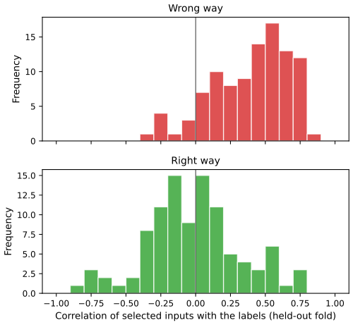
fig_7_10, screening_study. Reproduces Hastie, Tibshirani and Friedman (2009), Figure 7.10. Download: PDF · SVGThe predictors have an unfair advantage: they were chosen using all the samples, so leaving samples out after the selection does not imitate applying the classifier to new data; the selected predictors "have already seen" the held-out labels. The right procedure:
- Divide the samples into \(K\) folds at random.
- For each fold \(k=1,\dots,K\): (a) find the predictors most correlated with the labels using all samples except fold \(k\); (b) build the classifier on those predictors with the same samples; (c) predict the labels of fold \(k\).
- Accumulate the errors of step 2(c) over the folds.
Filling the gap 7.8: what cross-validation estimates, and why the order matters pp. 245–247
Let \(\mathcal A\) be the whole procedure (screening and fitting) that maps a training set to a classifier. If the folds are formed at random and \(\mathcal A\) is applied to each training part without using the held-out part, then for each held-out observation \((x_i,y_i)\) is a fresh draw from \(F\), independent of the classifier \(\mathcal A(\cT^{-\kappa(i)})\), and
\[ \E\,\CV=\E\,\Err\big(\mathcal A\text{ trained on }N(K-1)/K\text{ points}\big). \]If step (1) uses the held-out labels, the held-out pair is no longer independent of the classifier and this identity fails: the expectation is that of a different and (here) fictitious procedure.
Argument, and why unsupervised screening is harmless
For a fixed fold, \(\cT^{-k}\) and the held-out pairs are independent samples from \(F\) (random assignment of exchangeable observations), and \(\mathcal A(\cT^{-k})\) is a function of \(\cT^{-k}\) only. So \[ \E[L(y_i,\mathcal A(\cT^{-k})(x_i))\given\cT^{-k}]=\Err_{\cT^{-k}}, \] and averaging over training parts gives the expected error at training size \(N(K-1)/K\). In the wrong way the screening set \(S(\cT)\) depends on \(y_i\); in the null example, each selected predictor's correlation with the labels is large over all 50 samples, and it stays large on any subset of them, which is Figure 7.10. A screening step that ignores the labels, for example keeping the 1000 predictors of largest variance across all 50 samples, is harmless in the null case: it is a function of the inputs only, and when the labels are independent of the inputs, the held-out labels remain independent of everything the classifier was built from, so the expected CV error is the true 50%. The screening demo shows both ways giving about 50% under variance screening. ∎
In general, with a multistep modelling procedure, cross-validation must be applied to the entire sequence of steps, and samples must be left out before any selection or filtering that uses the labels. Initial unsupervised screening is allowed. The book notes that the blunder appears often in published work; see Ambroise and McLachlan (2002).
7.10.3 Does Cross-Validation Really Work?
pp. 247–249 A second high-dimensional null example: \(N=20\) samples in two classes of 10, \(p=500\) standard Gaussian predictors independent of the labels, and the classifier is a stump, a single split on one predictor chosen to minimise the training misclassification. A plausible-sounding argument says CV must fail: on all 20 samples we find a predictor that splits the data very well, the same predictor should split any 4/5 and 1/5 of the data well, so its CV error is small. Figure 7.11 shows that the argument is wrong.
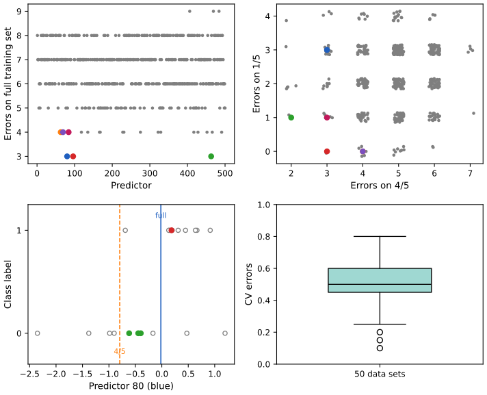
fig_7_11. Reproduces Hastie, Tibshirani and Friedman (2009), Figure 7.11. Download: PDF · SVGThe argument forgot that in cross-validation the model must be completely retrained in each fold: both the choice of predictor and its split point are re-estimated on the 4/5 part. Since the labels are independent of the predictors, a stump's performance on the 4/5 part carries no information about its performance on the other 1/5 (top right), and the refitted split point does not inherit the luck of the full-data one (bottom left). CV then behaves as it should, centred at 50%; but its spread across data sets is large, which is a reason always to report the standard error of a CV estimate. Exercise 7.10 takes away the split points as well, and CV still works.
7.11 Bootstrap Methods
pp. 249–252 The bootstrap (Efron, 1979) assesses statistical accuracy by resampling. From the training set \(\mathbf Z=(z_1,\dots,z_N)\), \(z_i=(x_i,y_i)\), draw \(B\) samples of size \(N\) with replacement, \(\mathbf Z^{*1},\dots,\mathbf Z^{*B}\), refit on each, and study the \(B\) replications \(S(\mathbf Z^{*b})\) of any statistic \(S\) (the book's Figure 7.12 is a schematic of this, not reproduced). For example,
\[ \widehat\Var[S(\mathbf Z)]=\frac1{B-1}\sum_{b=1}^B\big(S(\mathbf Z^{*b})-\bar S^*\big)^2,\qquad\bar S^*=\frac1B\sum_bS(\mathbf Z^{*b}), \tag{7.53} \]a Monte Carlo approximation of the variance of \(S\) when the data are drawn from the empirical distribution \(\hat F\) of \((z_1,\dots,z_N)\). A first idea for prediction error is to fit on each bootstrap sample and score on the original training set:
\[ \widehat\Err_{\rm boot}=\frac1B\frac1N\sum_{b=1}^B\sum_{i=1}^NL\big(y_i,\hf^{*b}(x_i)\big). \tag{7.54} \]This is not a good estimate: the training samples (bootstrap) and the test sample (original) share observations, and an overfitting rule looks unrealistically good on the shared ones. Cross-validation avoids exactly this by keeping training and test parts disjoint.
See also (companion course): Filling the gap 9.11 of Foundations of Deep Learning (what a bootstrap sample contains).
Result 7.14 (the 0.632 probability, and the naive bootstrap for 1-NN) p. 251, (7.55)
\[ \Pr\{\text{observation }i\in\text{bootstrap sample }b\}=1-\Big(1-\frac1N\Big)^N\approx1-e^{-1}=0.632. \tag{7.55} \]The left side decreases in \(N\) to its limit (0.75 at \(N=2\), 0.651 at \(N=10\), 0.634 at \(N=100\)), and a bootstrap sample contains on average \(N\{1-(1-1/N)^N\}\approx0.632N\) distinct observations. For 1-nearest neighbour on two equal classes with labels independent of the inputs, \(\E\widehat\Err_{\rm boot}=\tfrac12(1-1/N)^N\approx0.184\), while the true error is 0.5.
Proof
Each of the \(N\) draws misses observation \(i\) with probability \(1-1/N\), independently, so it is absent with probability \((1-1/N)^N\). Since \[ \log(1-1/N)^N=N\log(1-1/N)=-1-\frac1{2N}-\frac1{3N^2}-\cdots \] increases to \(-1\), \((1-1/N)^N\) increases to \(e^{-1}\) and the probability of inclusion decreases to \(1-e^{-1}\). The expected number of distinct observations is the sum over \(i\) of the inclusion probabilities. For 1-NN, an observation in the bootstrap sample is its own nearest neighbour (distance 0) and is classified correctly; an observation not in the sample gets the label of another observation, independent of its own, and is wrong with probability \(\tfrac12\). Hence \[ \E\widehat\Err_{\rm boot}=\tfrac12\Pr(i\notin\mathbf Z^{*b})=\tfrac12(1-1/N)^N\to0.5\times0.368=0.184. \] The value 0.184 is matched by the bootstrap demo. ∎
Mimicking cross-validation, the leave-one-out bootstrap uses for each observation only the bootstrap samples that do not contain it:
\[ \widehat\Err^{(1)}=\frac1N\sum_{i=1}^N\frac1{|C^{-i}|}\sum_{b\in C^{-i}}L\big(y_i,\hf^{*b}(x_i)\big), \tag{7.56} \]where \(C^{-i}\) is the set of bootstrap samples not containing \(i\) (choose \(B\) large enough that no \(C^{-i}\) is empty, or drop such terms). This removes the overfitting problem of (7.54) but has cross-validation's training-size bias: about \(0.632N\) distinct points per sample, so its bias behaves roughly like that of 2-fold CV, and if the learning curve is steep near \(N/2\) it overestimates the error. The .632 estimator pulls it toward the training error:
\[ \widehat\Err^{(.632)}=.368\cdot\err+.632\cdot\widehat\Err^{(1)}. \tag{7.57} \]Filling the gap 7.9: where the weight .632 comes from p. 251
The book calls the derivation "complex". Here is Efron's (1983) distance argument, with the assumptions under which it is exact. Suppose (i) the expected loss of a prediction at a point depends on the point only through its distance \(\delta\) to the nearest training input, and linearly: \(e(\delta)=e_0+c\,\delta\), with \(e_0\) the error at \(\delta=0\), i.e. the training error; and (ii) the inputs are uniform on an interval (one dimension, boundary effects ignored). Then
\[ \Err-\err\approx0.632\,\big(\widehat\Err^{(1)}-\err\big),\qquad\text{i.e.}\qquad\Err\approx0.368\,\err+0.632\,\widehat\Err^{(1)}. \]Derivation
With \(n\) uniform points, the distance from an independent uniform point to the nearest of them has mean about \(1/(2n)\) (two gaps of mean \(1/n\) on either side, each covered halfway on average). A new test point faces the \(N\) training inputs: \(\E\delta_{\rm test}\approx1/(2N)\). An observation left out of a bootstrap sample faces that sample's distinct points, about \(0.632N\) of them (Result 7.14), which are a random subset of the other observations and hence independent of it: \(\E\delta_{\rm OOB}\approx1/(2\cdot0.632N)\). So \(\E\delta_{\rm test}\approx0.632\,\E\delta_{\rm OOB}\). By (i), \(\Err-e_0=c\,\E\delta_{\rm test}\) and \(\widehat\Err^{(1)}-e_0\approx c\,\E\delta_{\rm OOB}\); with \(e_0=\err\) this is the claim. A simulation with \(N=100\) gives the ratio \(\E\delta_{\rm test}/\E\delta_{\rm OOB}=0.636\). The argument also shows when .632 fails: if the error does not grow with distance but jumps (1-NN with uninformative labels: error 0 at distance 0, \(\tfrac12\) at any positive distance), \(\Err=\widehat\Err^{(1)}=\tfrac12\) while \(\err=0\), and (7.57) gives \(0.632\times0.5=0.316\). This is the example due to Breiman et al. (1984) that motivates the next estimator. ∎
The .632 estimator works well in "light fitting" situations and breaks down in overfit ones such as the 1-NN example. Efron and Tibshirani (1997) improve it by measuring the amount of overfitting. The no-information error rate \(\gamma\) is the error of the rule when inputs and labels are independent; it is estimated by applying the fitted rule to all \(N^2\) combinations of responses and inputs:
\[ \hat\gamma=\frac1{N^2}\sum_{i=1}^N\sum_{i'=1}^NL\big(y_i,\hf(x_{i'})\big). \tag{7.58} \]For two classes, with \(\hat p_1\) the proportion of responses equal to 1 and \(\hat q_1\) the proportion of predictions \(\hf(x_{i'})\) equal to 1,
\[ \hat\gamma=\hat p_1(1-\hat q_1)+(1-\hat p_1)\hat q_1, \tag{7.59} \]because a pair \((i,i')\) is an error exactly when \(y_i=1,\hf(x_{i'})=0\) or \(y_i=0,\hf(x_{i'})=1\), and the double sum factorises into the product of the two marginal proportions. For a rule like 1-NN, \(\hat q_1=\hat p_1\) and \(\hat\gamma=2\hat p_1(1-\hat p_1)\); with \(K\) classes \(\hat\gamma=\sum_\ell\hat p_\ell(1-\hat q_\ell)\). The relative overfitting rate
\[ \hat R=\frac{\widehat\Err^{(1)}-\err}{\hat\gamma-\err} \tag{7.60} \]is 0 with no overfitting (\(\widehat\Err^{(1)}=\err\)) and 1 when the overfitting is as large as the no-information value. The .632+ estimator is
\[ \widehat\Err^{(.632+)}=(1-\hat w)\cdot\err+\hat w\cdot\widehat\Err^{(1)},\qquad\hat w=\frac{.632}{1-.368\hat R}. \tag{7.61} \]The weight runs from .632 at \(\hat R=0\) to 1 at \(\hat R=1\), so the estimate runs from \(\widehat\Err^{(.632)}\) to \(\widehat\Err^{(1)}\). In practice two safeguards are used (Efron and Tibshirani, 1997, and in the code here): \(\widehat\Err^{(1)}\) is replaced by \(\min(\widehat\Err^{(1)},\hat\gamma)\), and \(\hat R\) is set to 0 unless \(\widehat\Err^{(1)}>\err\) and \(\hat\gamma>\err\), which keeps \(\hat R\in[0,1]\).
Filling the gap 7.10: one way to see the .632+ weight p. 252
The weight \(\hat w=.632/(1-.368\hat R)\) is the solution of a fixed-point equation obtained from the .632 rule by correcting its training-error part for overfitting.
Derivation
The .632 rule \(\Err\approx.368\,\err+.632\,\widehat\Err^{(1)}\) uses the training error as the error "at distance 0". For a rule that overfits, the error of points that are in the training set says little about the error of a new point; replace \(\err\) in the .368 term by a value moved a fraction \(\hat R\) of the way from \(\err\) toward the target \(\Err\): \[ \Err\approx.368\{\err+\hat R(\Err-\err)\}+.632\,\widehat\Err^{(1)}. \] Subtracting \(\err\) from both sides, \[ (\Err-\err)(1-.368\hat R)=.632(\widehat\Err^{(1)}-\err), \] i.e. \(\Err\approx\err+\hat w(\widehat\Err^{(1)}-\err)\) with \(\hat w=.632/(1-.368\hat R)\), which is (7.61). The two ends are right: no overfitting (\(\hat R=0\)) returns the .632 rule; complete overfitting (\(\hat R=1\)) returns \(\widehat\Err^{(1)}\). In the 1-NN null example, \(\err=0\), \(\hat\gamma\approx\tfrac12\) (balanced classes) and \(\widehat\Err^{(1)}\approx\tfrac12\), so \(\hat R\approx\hat w\approx1\) and \(\widehat\Err^{(.632+)}\approx0.5\), as it should be; in the demo the 30 simulated data sets give 0.485 on average, slightly low because \(\widehat\Err^{(1)}\) falls a little below \(\hat\gamma\) in some of them. This is a motivation, not a derivation from first principles: Efron and Tibshirani justify the formula by its behaviour in simulations. ∎
7.11.1 Example (Continued)
pp. 252–254 Figure 7.13 repeats Figure 7.7 with 10-fold cross-validation and the .632+ bootstrap as the selection criteria.
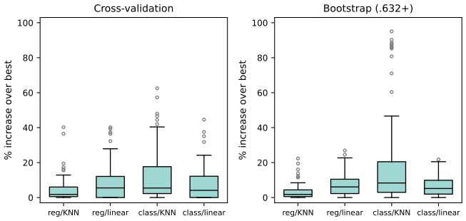
fig_7_13. Reproduces Hastie, Tibshirani and Friedman (2009), Figure 7.13. Download: PDF · SVGFor choosing a model, all of AIC, CV and the bootstrap land close to the best available model in these problems, as the book concludes; only relative sizes matter for selection, so a common bias in a criterion is harmless. For adaptive methods such as trees the effective number of parameters is very hard to estimate, which leaves cross-validation and the bootstrap as the practical choices.
How well each criterion estimates the error of the model it chose is another question. Averaged over the training sets, the value of the criterion at its chosen model differed from that model's test error by the following percentages (positive: overestimate):
| criterion | reg/KNN | reg/linear | class/KNN | class/linear |
|---|---|---|---|---|
| AIC | −7.8 | −16.6 | −40.4 | −71.5 |
| BIC | 4.7 | 3.6 | −30.0 | −59.4 |
| 10-fold CV | −7.2 | −6.7 | −20.8 | −10.6 |
| .632+ bootstrap | −0.4 | 10.0 | 5.3 | 17.3 |
The book reports that AIC overestimated by 38%, 37%, 51% and 30% and CV by 1%, 4%, 0% and 4%. Two things explain why my numbers differ. The level of an in-sample criterion depends entirely on \(\hat\sigma^2\), which the book specifies only loosely; with the recipe used here, \(\hat\sigma^2=[N/(N-d)]\err\) of the least restrictive model, the penalty is small, especially for the 0–1 loss, and AIC sits below the test error. And the minimum of a noisy curve is biased downward (Filling the gap 7.2): choosing \(k\) among 50 values on the CV curve makes the minimum CV value optimistic for the chosen model, most visibly for class/KNN. The book's warning stands in either case: when a reliable estimate of test error is needed, the search over models should itself be cross-validated (nested CV), or a separate test set kept; for trees the book reports that CV and the bootstrap can underestimate by 10% for this reason.
7.12 Conditional or Expected Test Error?
pp. 254–257 Does cross-validation estimate \(\Err_\cT\), the error of the model fitted to the training set at hand, or the expected error \(\Err\)? Figures 7.14 and 7.15 study this in the "reg/linear" scenario, which of the four gave the highest correlation between actual and predicted error.
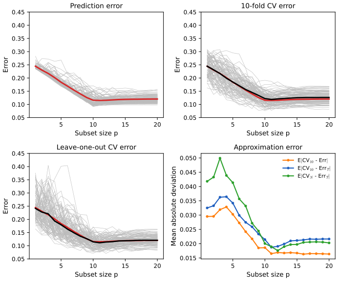
fig_7_14. Reproduces Hastie, Tibshirani and Friedman (2009), Figure 7.14. Download: PDF · SVGOne might have expected leave-one-out to track \(\Err_\cT\), since each of its fits uses almost the whole training set, and 10-fold CV to track \(\Err\), since its training sets differ more. The figure shows the opposite of the first expectation: neither estimates \(\Err_\cT\) well, and both are approximately unbiased for \(\Err\), with 10-fold having the smaller variance here. Similar trends were reported by Efron (1983).
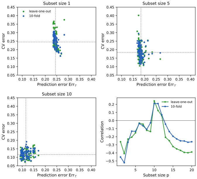
fig_7_15. Reproduces Hastie, Tibshirani and Friedman (2009), Figure 7.15. Download: PDF · SVGTwo features stand out: the CV estimates vary far more across training sets than the conditional errors do, and the two are nearly uncorrelated, mostly slightly negatively, a curious phenomenon observed before. The book adds that the same happens for bootstrap estimates and, it guesses, for any estimate of conditional error. The next result shows that in the simplest models zero correlation is not an accident but exact.
Result 7.15 (in a correct Gaussian linear model, CV carries no information about \(\Err_\cT\))
Let \(\by=\bX\beta+\be\), \(\be\sim N(0,\sigma^2\bI)\), with a fixed \(N\times p\) design of full rank, fitted by least squares, and let new inputs come from any distribution independent of \(\cT\). Then leave-one-out CV and GCV are independent of the conditional error \(\Err_\cT\) (and of the conditional in-sample error). For the location model (\(\bX=\mathbf 1\), \(\hf=\bar y\)) the same holds for \(K\)-fold CV with any fixed folds, and
\[ \Err_\cT=\sigma^2+(\bar y-\mu)^2,\qquad \CV_N=\frac N{(N-1)^2}\sum_{i=1}^N(y_i-\bar y)^2,\qquad \E\,\CV_N=\sigma^2\Big(1+\frac1{N-1}\Big), \]so \(\CV_N\) is exactly unbiased for the expected error of a training set of size \(N-1\) and uncorrelated with \(\Err_\cT\).
Proof
The residual vector \(\mathbf e=(\bI-\bH)\by=(\bI-\bH)\be\) and the estimation error \(\hat\beta-\beta=(\bX^\T\bX)^{-1}\bX^\T\be\) are jointly Gaussian with cross-covariance \(\sigma^2(\bI-\bH)\bX(\bX^\T\bX)^{-1}=0\), hence independent. By Result 7.13, \(\CV_N=\frac1N\sum_ie_i^2/(1-h_{ii})^2\) is a function of \(\mathbf e\), and so is \(\GCV=\frac1N\|\mathbf e\|^2/(1-p/N)^2\). The conditional error is \(\Err_\cT=\sigma^2+\E_{x_0}[(x_0^\T(\hat\beta-\beta))^2]\), a function of \(\hat\beta-\beta\) (and similarly the in-sample error, \(\sigma^2+\|\bX(\hat\beta-\beta)\|^2/N\)). Functions of independent variables are independent. For the location model, \(\bar y-\mu=\bar\varepsilon\) and every \(y_i-\bar y_{-k}\) is a linear function of the deviations \(y_j-\bar y\) (since \(\bar y_{-k}-\bar y=\frac{n_k}{N-n_k}(\bar y-\bar y_k)\)), which are independent of \(\bar y\). Finally \(y_i-\bar y_{-i}=\frac N{N-1}(y_i-\bar y)\) gives the formula for \(\CV_N\), and \(\E\sum_i(y_i-\bar y)^2=(N-1)\sigma^2\) gives \(\E\,\CV_N=N\sigma^2/(N-1)\), which is \(\sigma^2(1+\frac1{N-1})\), the expected error \(\E[\sigma^2+(\bar y_{N-1}-\mu)^2]\) of a mean of \(N-1\) observations. Both independence statements were confirmed by simulation (correlations of order \(10^{-3}\)). ∎
So, given only the training data, CV cannot tell a lucky training set from an unlucky one: what makes \(\Err_\cT\) large (the noise projected onto the model space) is invisible in the residuals, from which CV is computed. With model misspecification and data-driven selection, as in Figure 7.15, the independence breaks and weak, mostly negative, correlations appear. The conclusion is the book's: estimating the test error of a particular training set from that same training set is not possible in general; cross-validation and related methods estimate the expected error \(\Err\) reasonably.
Notes on the book
Four places where the printed text needs a correction, and three where my reproduction differs from the book's numbers for reasons I can only partly identify. Each correction was checked numerically.
Page 224: the ridge weights need an inverse, not a transpose
The text gives the linear weights of ridge regression as \(\bh(x_0)=\bX(\bX^\T\bX+\alpha\bI)^\T x_0\). Since \(\hf_\alpha(x_0)=x_0^\T(\bX^\T\bX+\alpha\bI)^{-1}\bX^\T\by\), the weights are \(\bh(x_0)=\bX(\bX^\T\bX+\alpha\bI)^{-1}x_0\), the analogue of \(\bX(\bX^\T\bX)^{-1}x_0\) in (7.11). (The printed expression is not even correct dimensionally unless read as a typo for the inverse.)
Page 229: for the deviance, (7.21) holds with the fitted log-odds, not the fitted probability
After (7.21) the book says that for entropy loss \(\hy_i\in[0,1]\) is the fitted probability of class 1. For the binomial deviance the exact identity is \(\omega=\frac2N\sum_i\Cov(\hat\theta_i,y_i)\) with \(\hat\theta_i=\log\{\hat p_i/(1-\hat p_i)\}\), the fitted natural parameter (Result 7.6(c)). With the probabilities in its place the formula can be badly off: in an exact enumeration of all \(2^{10}\) outcomes for a smoothed-proportion classifier, the true average optimism of the deviance is 0.306, the log-odds version gives 0.306, and the probability version gives 0.067.
Page 233: (7.34) needs the penalty \(\tfrac\alpha2\sum w_m^2\)
With the penalty \(\alpha\sum_mw_m^2\) as written and \(\theta_m\) the eigenvalues of the Hessian of \(R\), the trace of the linearised smoother is \(\sum_m\theta_m/(\theta_m+2\alpha)\). Formula (7.34) is right for the penalty \(\tfrac\alpha2\sum_mw_m^2\), the convention of Bishop (1995) from which it is taken (Filling the gap 7.5). For ridge regression with \(\alpha=3\) on a random design, the trace is 3.748; \(\sum\theta/(\theta+2\alpha)=3.748\); the printed formula gives 3.870.
Page 236: (7.45) is missing a factor \(\tfrac12\)
For \(y\sim N(\theta,\sigma^2)\) and \(\theta\sim N(0,1)\), \[ -\log\Pr(y\given\theta)-\log\Pr(\theta)=\log(2\pi)+\log\sigma+\frac{(y-\theta)^2}{2\sigma^2}+\frac{\theta^2}2. \] The book prints \((y-\theta)^2/\sigma^2\), which is inconsistent with the \(\theta^2/2\) next to it.
Where my numbers differ from the book's
- Section 7.10.2. The wrong-way CV error averages 1.6% here and 3% in the book; the held-out correlations average 0.36 here and "about 0.28" in the book. The book does not say how the 100 predictors were ranked or how the correlations in Figure 7.10 were signed; with signed correlations of predictors ranked by absolute correlation the mean would be near 0, so some sign convention is needed, and the value depends on it. The qualitative conclusion is unaffected.
- Section 7.11.1. The book reports that AIC overestimated the error of its chosen model by 30–51% and CV by 0–4%; here AIC underestimates by 8–72% and CV by 7–21% (the table in Section 7.11.1). The AIC level depends on \(\hat\sigma^2\), which the book leaves partly unspecified; the CV underestimate is the selection effect of Filling the gap 7.2.
- Figure 7.4, right panel. The book's AIC curve for 0–1 loss implies a penalty of about \(d/N\) (\(\hat\sigma^2\approx\tfrac12\)); I used \(\hat\sigma^2=\tfrac14\), the largest variance of a 0/1 variable.
- A clarification, p. 224. "For linear models fit by ordinary least squares, the estimation bias is zero" is exact when the average in (7.14) is over the training inputs (or as \(N\to\infty\)); with a population average and finite \(N\), \(\E\hat\beta\) is the best linear fit for the training inputs, not \(\beta_*\) (Result 7.4).
Exercises
All 10 exercises of Chapter 7 (Hastie, Tibshirani and Friedman, 2009, pp. 257–259), restated in my own words, with complete solutions (hidden).
Exercise 7.1. Derive the in-sample error estimate (7.24).
Solution
Let \(\hat\by=\bH\by\) with \(\bH\) a fixed projection of rank \(d\), \(\by=\bf+\be\), \(\E\be=0\), \(\Cov\be=\sigma^2\bI\), and \(\by^0=\bf+\be^0\) new responses at the same inputs, independent of \(\by\). For any fixed matrix \(\mathbf A\), \[ \E\|\mathbf A\by\|^2=\|\mathbf A\bf\|^2+\sigma^2\Tr(\mathbf A^\T\mathbf A). \] Training error: \(\by-\hat\by=(\bI-\bH)\by\) and \((\bI-\bH)^\T(\bI-\bH)=\bI-\bH\), so \[ \E\err=\frac1N\{\|(\bI-\bH)\bf\|^2+\sigma^2(N-d)\}. \] In-sample error: \(\by^0-\hat\by=\be^0+(\bI-\bH)\bf-\bH\be\), three terms of which the first and last are independent with mean zero and the middle one is fixed, so \[ \E\Err_{\rm in}=\frac1N\{N\sigma^2+\|(\bI-\bH)\bf\|^2+\sigma^2\Tr\bH\}=\sigma^2+\frac1N\|(\bI-\bH)\bf\|^2+\frac dN\sigma^2. \] Subtracting, \(\E\Err_{\rm in}-\E\err=\frac{2d}N\sigma^2\), which is (7.24). The same result follows from (7.22) and \(\sum_i\Cov(\hy_i,y_i)=\sigma^2\Tr\bH=d\sigma^2\) (Result 7.7). Notice that the model may be wrong (\(\bH\bf\ne\bf\)): the bias terms cancel.
Exercise 7.2. For 0–1 loss with \(Y\in\{0,1\}\) and \(\Pr(Y=1\given x_0)=f(x_0)\), show (7.62), where \(\hat G(x)=I(\hf(x)>\tfrac12)\), \(G(x)=I(f(x)>\tfrac12)\) is the Bayes rule and \(\Err_B(x_0)\) the Bayes error at \(x_0\). Then, approximating \(\hf(x_0)\) by a Gaussian with the same mean and variance, show (7.63).
Solution
This is Result 7.5, proved there. The key steps: conditional on \(\hat G\), the error probability is \(1-f\) or \(f\); writing \(\Pr(\hat G=1)\) or \(\Pr(\hat G=0)\) as \(\Pr(\hat G\ne G)\) on each side of \(\tfrac12\) gives \(\Err=\Err_B+|2f-1|\Pr(\hat G\ne G)\); and \(\Pr(\hat G\ne G)\) is a Gaussian tail probability on the side of \(\tfrac12\) opposite to \(f\), which (7.63) writes with the sign factor. The interpretation (bias and variance combine multiplicatively; on the wrong side of the boundary a larger variance helps) is discussed there. Numerically, with \(f=0.7\), \(\E\hf=0.45\), \(\mathrm{sd}=0.12\), simulation gives \(\Pr(\hat G\ne G)=0.661\) against \(\Phi(0.05/0.12)=0.662\).
Exercise 7.3. Let \(\hf=\bS\by\) be a linear smoother. (a) For least squares projections and cubic smoothing splines, show that the leave-one-out residual is \[ y_i-\hf^{-i}(x_i)=(y_i-\hf(x_i))/(1-S_{ii}), \] (7.64). (b) Deduce \(|y_i-\hf^{-i}(x_i)|\ge|y_i-\hf(x_i)|\). (c) Find general conditions on a smoother for (7.64) to hold.
Solution
(a) Both are penalised least-squares fits over a fixed class (\(J=0\) for least squares, \(J=\lambda\int g''^2\) over the natural cubic splines with knots at the data for smoothing splines, see Result 5.9). By Result 7.13 they are self-stable: the leave-one-out minimiser also minimises the full criterion once \(y_i\) is replaced by its own leave-one-out prediction. One small point for splines: after removing \(x_i\) the natural spline space with knots at the remaining points is smaller, but the minimiser over all twice-differentiable functions of the leave-one-out criterion is a natural spline with knots at the remaining points, which is also a natural spline with knots at all points; so working in the full space loses nothing. The identity then follows by solving \(\hf^{-i}(x_i)=\sum_{j\ne i}S_{ij}y_j+S_{ii}\hf^{-i}(x_i)\). (b) Projections and smoothing-spline smoothers are symmetric with eigenvalues in \([0,1]\), so \(0\le S_{ii}\le1\); if \(S_{ii}\lt 1\) then \(|1-S_{ii}|\le1\) and the inequality follows. (If \(S_{ii}=1\) the fit interpolates \(y_i\) and the leave-one-out residual is not determined by (7.64).) (c) The general condition is self-stability: \(\hf^{-i}(x_i)=(\bS\tilde\by)_i\), where \(\tilde\by\) is \(\by\) with \(y_i\) replaced by \(\hf^{-i}(x_i)\). It holds for every penalised (or weighted) least-squares fit over a class that does not depend on the data points, including Nadaraya–Watson and local polynomial regression with a fixed metric window, and fails when removing a point changes the other points' weights, as for \(k\)-nearest neighbours or nearest-neighbour windows.
Exercise 7.4. For squared error, write \(\Err_{\rm in}=\frac1N\sum_i\E_{Y^0}(Y_i^0-\hf(x_i))^2\) and \(\err=\frac1N\sum_i(y_i-\hf(x_i))^2\). Add and subtract \(f(x_i)\) and \(\E\hf(x_i)\) in each, expand, and show that the average optimism is \(\frac2N\sum_i\Cov(\hy_i,y_i)\).
Solution
Write \(f_i=f(x_i)\), \(\bar f_i=\E\hf(x_i)\), \(\hy_i=\hf(x_i)\), \(\varepsilon_i=y_i-f_i\). Then \(Y_i^0-\hy_i=\varepsilon_i^0+(f_i-\bar f_i)+(\bar f_i-\hy_i)\) and \(y_i-\hy_i=\varepsilon_i+(f_i-\bar f_i)+(\bar f_i-\hy_i)\). Taking expectations of the squares (over \(Y^0\) and \(\by\)), the squares give \(\sigma^2+(f_i-\bar f_i)^2+\Var\hy_i\) in both. The cross terms: in the in-sample case all vanish, because \(\varepsilon_i^0\) is independent of \(\hy_i\) and \(\E(\bar f_i-\hy_i)=0\). In the training case, \(2\E[\varepsilon_i(f_i-\bar f_i)]=0\) and \(2\E[(f_i-\bar f_i)(\bar f_i-\hy_i)]=0\), but \[ 2\E[\varepsilon_i(\bar f_i-\hy_i)]=-2\E[\varepsilon_i\hy_i]=-2\Cov(y_i,\hy_i). \] Hence \[ \E_\by(\Err_{\rm in}-\err)=\frac2N\sum_i\Cov(\hy_i,y_i). \] This is Result 7.6(a), which also covers 0–1 loss and the deviance.
Exercise 7.5. For a linear smoother \(\hat\by=\bS\by\), show (7.65), \(\sum_i\Cov(\hy_i,y_i)=\Tr(\bS)\sigma_\varepsilon^2\), which justifies \(\Tr\bS\) as the effective number of parameters.
Solution
\[ \Cov(\hat\by,\by)=\Cov(\bS\by,\by)=\bS\Cov(\by)=\sigma_\varepsilon^2\bS \] because \(\bS\) does not depend on \(\by\); the diagonal entries are \(\Cov(\hy_i,y_i)=\sigma_\varepsilon^2S_{ii}\), and summing gives the trace (Result 7.8). With (7.22), Cp with \(d=\Tr\bS\) is then unbiased for the in-sample error, which is what makes the trace the right replacement for \(d\). Only uncorrelated, equal-variance errors are needed, not Gaussianity. A simulation with ridge regression gave 5.205 against \(\Tr\bS=5.207\).
Exercise 7.6. Show that, for an additive-error model, the effective degrees of freedom of \(k\)-nearest-neighbour regression is \(N/k\).
Solution
The \(k\)-NN fit at a training input averages the \(k\) nearest training responses, and the point itself, at distance 0, is one of them (the usual convention; ties ignored). So \(\hat\by=\bS\by\) with \(S_{ij}=1/k\) if \(x_j\) is among the \(k\) nearest neighbours of \(x_i\) and 0 otherwise, a matrix that depends on the inputs only. Its diagonal is \(S_{ii}=1/k\) for every \(i\), so \(\Tr\bS=N/k\), and by Exercise 7.5 \(\sum_i\Cov(\hy_i,y_i)/\sigma_\varepsilon^2=N/k\). Intuitively, the data are cut into about \(N/k\) neighbourhoods with one mean each. (If a point were excluded from its own neighbourhood the trace would be 0, which is why the convention matters; see also Result 2.2.) Note that \(\bS\) is not symmetric, so its eigenvalues need not lie in \([0,1]\), but the trace argument does not need that.
Exercise 7.7. Use \(1/(1-x)^2\approx1+2x\) to relate Cp/AIC (7.26) to GCV (7.52); the main difference is the model used to estimate the noise variance.
Solution
With \(x=\Tr(\bS)/N\), \(\GCV=\err/(1-x)^2\), and \(1/(1-x)^2=1+2x+3x^2+\cdots\), so \(\GCV=\err+2\frac{\Tr\bS}N\err+O(x^2)\). Compare \(C_p=\err+2\frac{\Tr\bS}N\hat\sigma^2\): the two coincide to first order in \(\Tr\bS/N\) if \(\hat\sigma^2=\err\). So GCV is Cp with the noise variance estimated by the training error of the model being assessed, while Cp uses one estimate, from a low-bias model, for all models. For a model with large bias, \(\err\) overestimates \(\sigma^2\) and GCV penalises it more; for a flexible model \(\err\) underestimates \(\sigma^2\) but the exact factor \(1/(1-x)^2\) grows faster than \(1+2x\) and compensates. The remainder is at most \(\err\cdot\frac{(3-2x)x^2}{(1-x)^2}\le4\err\,x^2/(1-x)^2\) for \(0\le x\le\tfrac12\); a computation confirmed it for a penalised spline.
Exercise 7.8. Show that \(\{I(\sin(\alpha x)>0)\}\) shatters the points \(z_\ell=10^{-\ell}\), \(\ell=1,\dots,L\), for every \(L\); hence its VC dimension is infinite.
Solution
Given labels \(y_1,\dots,y_L\in\{0,1\}\), take \(\alpha=\pi\big(1+\sum_{i=1}^L(1-y_i)10^i\big)\). Then for each \(j\),
\[ \frac{\alpha z_j}\pi=10^{-j}+\sum_{i\lt j}(1-y_i)10^{i-j}+(1-y_j)+\sum_{i>j}(1-y_i)10^{i-j}. \]The last sum is an integer multiple of \(10\), hence even, and contributes nothing to \(\sin\). The first two terms form \(\epsilon_j=10^{-j}+\sum_{i\lt j}(1-y_i)10^{i-j}\), with \(0\lt \epsilon_j\le\sum_{m=1}^j10^{-m}\lt \tfrac19\). So \(\sin(\alpha z_j)=\sin\big(\pi(1-y_j)+\pi\epsilon_j\big)\). If \(y_j=1\) this is \(\sin(\pi\epsilon_j)>0\); if \(y_j=0\) it is \(\sin(\pi+\pi\epsilon_j)=-\sin(\pi\epsilon_j)\lt 0\). Thus \(I(\sin(\alpha z_j)>0)=y_j\) for every \(j\): every labelling of \(L\) points is realised, for every \(L\), and the VC dimension is infinite. An exact (rational-arithmetic) check confirmed all \(2^L\) labellings for \(L\le10\). The one-parameter family is therefore more complex, in the VC sense, than any finite-dimensional linear class, the point of Figure 7.5.
Exercise 7.9. For the prostate data of Chapter 3, carry out best-subset linear regression as in Table 3.3 (third column). Compute AIC, BIC, five- and tenfold cross-validation, and bootstrap .632 estimates of prediction error, and discuss.
Solution
Method. The 67 training cases with the 8 inputs standardised as in the book; for each size \(k=0,\dots,8\) the best subset by exhaustive search; \(\hat\sigma^2=0.507\), the residual variance of the full model (\(N-9\) degrees of freedom); AIC \(=\err+2d\hat\sigma^2/N\) and BIC \(=\err+(\log N)d\hat\sigma^2/N\) with \(d=k+1\); CV and the bootstrap redo the best-subset search inside every fold or bootstrap sample (the right way); \(B=200\) bootstrap samples; the 30 test cases give an independent check. Code:
prostate_selection.\(k\) best subset \(\err\) AIC BIC CV5 CV10 .632 test 0 (none) 1.437 1.452 1.469 1.539 1.467 1.479 1.057 1 lcavol 0.665 0.695 0.728 0.712 0.704 0.719 0.480 2 + lweight 0.554 0.599 0.649 0.612 0.660 0.655 0.492 3 + svi 0.521 0.582 0.648 0.696 0.668 0.656 0.401 4 + lbph 0.490 0.566 0.649 0.653 0.622 0.646 0.456 5 + pgg45 0.479 0.570 0.670 0.697 0.687 0.635 0.486 6 + lcp 0.456 0.562 0.679 0.703 0.629 0.614 0.549 7 + age 0.439 0.561 0.694 0.640 0.555 0.594 0.517 8 + gleason 0.439 0.576 0.726 0.635 0.561 0.589 0.521 (The subsets are nested here; the size-2 model and its test error 0.492, and the full model's 0.521, agree with Table 3.3.)
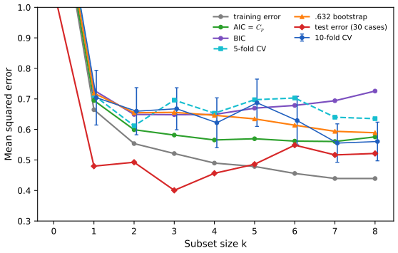
Figure 7.S2 (supplementary, Exercise 7.9). The estimates of the table against subset size; bars on 10-fold CV are one standard error. Code: fig_7_s2. Download: PDF · SVGDiscussion. (i) Every criterion drops sharply from \(k=0\) to \(k=2\) and is nearly flat after that: the differences between sizes 2 and 8 (about 0.05–0.1) are below one standard error of CV (about 0.07–0.08), so the data do not distinguish these models. (ii) The minimisers disagree: AIC 7, BIC 3, CV5 2, CV10 7, .632 8. BIC's heavier penalty points to a smaller model, as expected (Result 7.10); the .632 estimator, whose training-error part favours the largest model, picks the full model. (iii) CV is noisy with only 67 cases: changing from 5 to 10 folds moves the minimum from 2 to 7. The one-standard-error rule with 5-fold CV keeps \(k=2\), the choice of Table 3.3 (which used 10-fold CV with the rule and different random folds); with these 10 folds it keeps \(k=7\). Repeating CV over several random partitions, and applying the one-standard-error rule, is advisable. (iv) As estimates of the error level, all of them are above the test error of the 30 held-out cases (0.40–0.55); the test set is small (its standard errors are about 0.1–0.15), so this reflects chance as much as bias. (v) Since the subsets are chosen by a search, AIC with \(d=k+1\) understates the optimism (Filling the gap 7.4); with only 8 inputs the effect is moderate, and the optimism demo estimates it for forward stepwise on this design.
Exercise 7.10. In the setting of Section 7.10.3, suppose all \(p\) predictors are binary, so there are no split points to estimate, and independent of the labels. With \(p\) very large there is probably a predictor that splits the whole training set perfectly, and it would then split each validation fold perfectly too, giving zero CV error. Does this mean CV fails here?
Solution
No. The argument evaluates, in every fold, the predictor chosen on all the data, which is the wrong way of Section 7.10.2. Done correctly, each fold re-selects the predictor from its own training part, and then CV is exactly unbiased for the error of the procedure, which is \(\tfrac12\).
Exact argument. Let the predictors be independent fair bits, independent of the labels. In fold \(k\), the chosen predictor \(J_k\) (fewest training errors, ties broken by index, either orientation) is a function of the training part only. The held-out values \(x_{iJ_k}\), \(i\) in fold \(k\), are fair bits independent of the training part and of the held-out labels (they are entries of other rows), so each held-out prediction is correct with probability exactly \(\tfrac12\), whatever \(J_k\) is. Hence \(\E\,\CV=\tfrac12\). The intuitive reason the perfect splitter does not help: with \(N=20\) and 5 folds, a predictor that splits the 16 training samples perfectly is one of roughly \(p\cdot2\cdot2^{-16}\) such predictors, of which only a fraction \(2^{-4}\) also split the 4 held-out samples perfectly; the fold has no way to tell which.
Simulation. \(N=20\) (10 per class), \(p=2^{20}\approx10^6\) random binary predictors, 50 data sets (
binary_stump_cv): 45 of the 50 contain a predictor that splits all 20 samples perfectly (the chance is \(1-(1-2^{-19})^{p}\approx0.86\)), yet 5-fold CV averages 0.497. CV gives a good estimate of the test error in this situation, though, as in Figure 7.11, with a large spread across data sets.
Demonstrations for this chapter
Each demonstration runs in the browser on the course's data files and links back to these notes. The ▶ Demo boxes above open them already set to the case under discussion.
| Demonstration | What you can see | Sections and results |
|---|---|---|
| Optimism, Cp and BIC | Monte Carlo on the prostate design: average training error, in-sample error, Cp and BIC by model size; the optimism against \(2d\sigma^2/N\); the effective degrees of freedom \(\sum\Cov(\hy_i,y_i)/\sigma^2\); how often each criterion picks each size; fixed order against forward stepwise, with up to 12 pure-noise inputs. Presets: 1 fixed order; 2 forward stepwise; 3 stepwise with noise inputs; 4 fixed order with noise inputs; 5 AIC against BIC. | 7.4–7.7; Results 7.6–7.8, 7.10, Filling the gap 7.4 |
| Cross-validation the wrong and right way | 50 samples, up to 5000 null or partly informative inputs, correlation or variance screening, 1-NN, 5- or 10-fold CV done both ways, the test error of the final classifier, and the held-out correlations of Figure 7.10. Presets: 1 the book's experiment; 2 Figure 7.10; 3 fewer inputs, ten folds; 4 real signal; 5 unsupervised screening. | 7.10.2, 7.10.3; Filling the gap 7.8 |
| The .632 and .632+ bootstrap | \(k\)-NN classifiers on the Chapter 2 mixture or on uninformative labels; the training error, the naive bootstrap (7.54), the leave-one-out bootstrap (7.56), .632 (7.57), .632+ (7.61), 10-fold and leave-one-out CV against the exact error of each training set, accumulated over many training sets. Presets: 1 1-NN on the mixture; 2 no information; 3 15-NN; 4 small sample; 5 oversmoothing. | 7.11; Result 7.14, Filling the gaps 7.9, 7.10 |
Related demonstrations: in this course, the \(k\)-NN bias–variance demo of Chapter 2; in the companion courses, the bias–variance demo and the evidence demo of Bayesian and Probabilistic Machine Learning, and the model-selection demo of Foundations of Deep Learning. The Python code that produces every figure of this page is code/ch07_model_assessment.py (see the code index).
References
- Hastie, T., Tibshirani, R. and Friedman, J. (2009). The Elements of Statistical Learning: Data Mining, Inference, and Prediction, 2nd edition. Springer, New York. Chapter 7, pp. 219–260. hastie.su.domains/ElemStatLearn.
- Akaike, H. (1973). Information theory and an extension of the maximum likelihood principle. In Second International Symposium on Information Theory, 267–281. Akadémiai Kiadó, Budapest.
- Allen, D. M. (1974). The relationship between variable selection and data augmentation and a method for prediction. Technometrics, 16(1), 125–127.
- Ambroise, C. and McLachlan, G. J. (2002). Selection bias in gene extraction on the basis of microarray gene-expression data. Proceedings of the National Academy of Sciences, 99(10), 6562–6566.
- Bengio, Y. and Grandvalet, Y. (2004). No unbiased estimator of the variance of K-fold cross-validation. Journal of Machine Learning Research, 5, 1089–1105.
- Bishop, C. M. (1995). Neural Networks for Pattern Recognition. Clarendon Press, Oxford.
- Breiman, L. and Spector, P. (1992). Submodel selection and evaluation in regression: the X-random case. International Statistical Review, 60(3), 291–319.
- Breiman, L., Friedman, J., Olshen, R. and Stone, C. (1984). Classification and Regression Trees. Wadsworth, Belmont.
- Cherkassky, V. and Ma, Y. (2003). Comparison of model selection for regression. Neural Computation, 15(7), 1691–1714.
- Cherkassky, V. and Mulier, F. (2007). Learning from Data: Concepts, Theory, and Methods, 2nd edition. Wiley, Hoboken.
- Cover, T. M. and Thomas, J. A. (1991). Elements of Information Theory. Wiley, New York.
- Efron, B. (1979). Bootstrap methods: another look at the jackknife. The Annals of Statistics, 7(1), 1–26.
- Efron, B. (1983). Estimating the error rate of a prediction rule: improvement on cross-validation. Journal of the American Statistical Association, 78(382), 316–331.
- Efron, B. (1986). How biased is the apparent error rate of a prediction rule? Journal of the American Statistical Association, 81(394), 461–470.
- Efron, B. and Tibshirani, R. (1993). An Introduction to the Bootstrap. Chapman and Hall, London.
- Efron, B. and Tibshirani, R. (1997). Improvements on cross-validation: the .632+ bootstrap method. Journal of the American Statistical Association, 92(438), 548–560.
- Friedman, J. H. (1997). On bias, variance, 0/1-loss, and the curse-of-dimensionality. Data Mining and Knowledge Discovery, 1(1), 55–77.
- Furnival, G. M. and Wilson, R. W. (1974). Regressions by leaps and bounds. Technometrics, 16(4), 499–511.
- Golub, G. H., Heath, M. and Wahba, G. (1979). Generalized cross-validation as a method for choosing a good ridge parameter. Technometrics, 21(2), 215–223.
- Hastie, T., Tibshirani, R. and Friedman, J. (2003). A note on "Comparison of model selection for regression" by Cherkassky and Ma. Neural Computation, 15(7), 1477–1480.
- Kohavi, R. (1995). A study of cross-validation and bootstrap for accuracy estimation and model selection. In Proceedings of the 14th International Joint Conference on Artificial Intelligence, 1137–1143.
- Madigan, D. and Raftery, A. E. (1994). Model selection and accounting for model uncertainty in graphical models using Occam's window. Journal of the American Statistical Association, 89(428), 1535–1546.
- Ripley, B. D. (1996). Pattern Recognition and Neural Networks. Cambridge University Press, Cambridge.
- Rissanen, J. (1983). A universal prior for integers and estimation by minimum description length. The Annals of Statistics, 11(2), 416–431.
- Sauer, N. (1972). On the density of families of sets. Journal of Combinatorial Theory, Series A, 13(1), 145–147.
- Schwarz, G. (1978). Estimating the dimension of a model. The Annals of Statistics, 6(2), 461–464.
- Shannon, C. E. (1948). A mathematical theory of communication. Bell System Technical Journal, 27, 379–423 and 623–656.
- Stamey, T., Kabalin, J., McNeal, J., Johnstone, I., Freiha, F., Redwine, E. and Yang, N. (1989). Prostate specific antigen in the diagnosis and treatment of adenocarcinoma of the prostate II: radical prostatectomy treated patients. Journal of Urology, 141(5), 1076–1083.
- Stein, C. M. (1981). Estimation of the mean of a multivariate normal distribution. The Annals of Statistics, 9(6), 1135–1151.
- Stone, M. (1974). Cross-validatory choice and assessment of statistical predictions. Journal of the Royal Statistical Society, Series B, 36(2), 111–147.
- Stone, M. (1977). An asymptotic equivalence of choice of model by cross-validation and Akaike's criterion. Journal of the Royal Statistical Society, Series B, 39(1), 44–47.
- Vapnik, V. (1998). Statistical Learning Theory. Wiley, New York.
- Wahba, G. (1990). Spline Models for Observational Data. SIAM, Philadelphia.
- Zou, H., Hastie, T. and Tibshirani, R. (2007). On the "degrees of freedom" of the lasso. The Annals of Statistics, 35(5), 2173–2192.
The numerical statements in the text (the decompositions of Section 7.3, the optimism identities for squared error, 0–1 loss and the deviance, the degrees of freedom of ridge, \(k\)-NN and weight decay, AIC's correction, the Laplace approximation, Shannon's bound, the shattering results, the leave-one-out identity and GCV, the independence of CV from the conditional error, the 0.632 calculations, and the corrections listed in the notes on the book) were confirmed numerically.