Single-layer Networks: Regression
A linear regression model is the simplest neural network: one layer of adjustable weights between a set of fixed features and an output. Because the model is linear in its weights, everything can be computed in closed form: the maximum likelihood weights solve a linear system, the fitted values are an orthogonal projection, a quadratic penalty shrinks the weights along the directions the data determine least well, and a one-point-at-a-time version of the fit is the simplest instance of stochastic gradient descent. The chapter then asks two questions that recur throughout deep learning: which single prediction should be made from a predictive distribution (decision theory), and why a model that fits each training set well can still predict badly (the bias–variance trade-off).
Ch. 1 Deep learning revolution Ch. 2 Probabilities Ch. 3 Standard distributions Ch. 4 Regression Ch. 5 Classification Ch. 6 Deep neural networks Ch. 7 Gradient descent Ch. 8 Backpropagation Ch. 9 Regularization Ch. 10 Convolutional networks Ch. 11 Structured distributions Ch. 12 Transformers Ch. 13 Graph neural networks Ch. 14 Sampling Ch. 15 Discrete latent variables Ch. 16 Continuous latent variables Ch. 17 GANs Ch. 18 Normalizing flows Ch. 19 Autoencoders Ch. 20 Diffusion models Appendices A to C
How to read these notes
They follow the book. Sections carry the book's numbers (4.1, 4.1.3, ...) and every displayed equation that appears in the book carries the book's own equation number, e.g. \((4.14)\), so you can read these notes next to the book. Equations without a number are steps that the book skips.
Filling the gaps. Wherever the book says that a result "can easily be verified", leaves it to an exercise, or states a property without proof, an orange Filling the gap box or a proof gives the full argument. Proofs and derivations start hidden: open one with its bar, or use the button below.
Figures and demonstrations. Every figure of the chapter that is computed from data or a model is reproduced from scratch by the Python code; the two network diagrams are redrawn. The ▶ Demo boxes open an interactive demonstration already set to the case being discussed.
Main reference
C. M. Bishop and H. Bishop, Deep Learning: Foundations and Concepts, Springer (2024), Chapter 4, pages 111–130 (book website: www.bishopbook.com). Section, equation, figure and exercise numbers below refer to this book. Further reading is listed in the references.
The explanations, derivations, figures and code are my own; equations are cited by their numbers in the book.
Companion course
Most of this chapter also appears, in the language of Bishop (2006), in the companion course Bayesian and Probabilistic Machine Learning. The overlapping material is:
- Sections 4.1.1–4.1.7 (basis functions, maximum likelihood, geometry, sequential learning, ridge regression, multiple outputs): Chapter 3, Section 3.1, with the subsections 3.1.1–3.1.5.
- Section 4.2 (decision theory for regression, the Minkowski loss): Chapter 1, Section 1.5.5.
- Section 4.3 (the bias–variance trade-off, Figures 4.7 and 4.8): Chapter 3, Section 3.2, including a closed form for ridge regression and the link with the Bayesian choice of \(\lambda\).
- Exercise 4.3 (sigmoid and tanh units): Chapter 5, Filling the gap 5.2. Demonstrations of the same ideas: curve fitting, bias and variance, sequential Bayesian regression.
Where a proof there is identical, these notes give the statement and a short argument and link to it. New here: the role of the pseudo-inverse when the basis is degenerate, the conditioning of the normal equations, the convergence behaviour of LMS with a constant learning rate, the effect of penalising the bias, and a correction to the claim that the Minkowski loss gives the mode as \(q\to0\) (Result 4.11).
The chapter at a glance
- 4.1.1 A linear model \(y=\mathbf{w}^\T\bphi(\mathbf{x})\) is a network with one layer of weights on fixed features (Definition 4.1); sigmoid and tanh features span the same functions (Result 4.1).
- 4.1.2–4.1.3 Gaussian noise turns maximum likelihood into least squares; the solution is \(\mathbf{w}_{\rm ML}=\bPhi^\dagger\mathbf{t}\) (Results 4.2, 4.3), the bias absorbs the means, and \(\sigma^2_{\rm ML}\) is biased downwards by the factor \((N-M)/N\) (Result 4.4).
- 4.1.4 The fitted vector is the orthogonal projection of \(\mathbf{t}\) onto the span of the columns of \(\bPhi\) (Result 4.5); the normal equations square the condition number, which is why the SVD or a penalty is used (Filling the gap 4.4).
- 4.1.5 LMS is stochastic gradient descent; it converges for consistent data, hovers within \(O(\eta)\) of \(\mathbf{w}_{\rm ML}\) for noisy data, and needs a decreasing learning rate to converge (Result 4.6).
- 4.1.6–4.1.7 Ridge regression shrinks each singular direction by \(d_i^2/(d_i^2+\lambda)\) (Result 4.7); with several outputs the problem splits into independent problems, whatever the noise covariance (Result 4.8).
- 4.2 The squared loss is minimised by \(\E[t\given\mathbf{x}]\) (Result 4.9), the absolute loss by the median (Result 4.10), and the Minkowski loss with \(q\to0\) by the minimiser of \(\E\ln|f-t|\), which is the mode only in special cases (Result 4.11).
- 4.3 Expected loss = bias\(^2\) + variance + noise (Result 4.12); for ridge regression both terms are explicit (Result 4.13).
Notation. Inputs \(\mathbf{x}\in\R^D\), target \(t\in\R\) (or \(\mathbf{t}\in\R^K\)), data \(\{(\mathbf{x}_n,t_n)\}_{n=1}^N\) collected in the vector \(\mathbf{t}=(t_1,\dots,t_N)^\T\). Basis functions \(\phi_0\equiv1,\phi_1,\dots,\phi_{M-1}\), \(\bphi_n=\bphi(\mathbf{x}_n)\in\R^M\), design matrix \(\bPhi\in\R^{N\times M}\) with rows \(\bphi_n^\T\) and columns \(\bvphi_j\). Gradients are column vectors.
Prerequisites. The Gaussian distribution and maximum likelihood (Chapters 2 and 3 of the book), polynomial curve fitting (Section 1.2), and the matrix calculus and singular value decomposition of the companion course's toolkit.
4.1 Linear Regression
p. 112 In regression we observe \(N\) inputs \(\mathbf{x}_n\in\R^D\) with continuous targets \(t_n\) and want a function \(y(\mathbf{x},\mathbf{w})\) that predicts \(t\) at new inputs. The simplest choice is a linear function of the inputs,
\[ y(\mathbf{x},\mathbf{w})=w_0+w_1x_1+\dots+w_Dx_D, \tag{4.1} \]which is linear in the parameters (the property that makes everything below computable) but also linear in \(\mathbf{x}\), which is a severe restriction.
See also (companion course): Section 3.1, linear basis function models.
4.1.1 Basis functions
Definition 4.1 (linear basis function model) pp. 112–113, (4.2)–(4.6)
Fix functions \(\phi_1,\dots,\phi_{M-1}:\R^D\to\R\), the basis functions, and the constant \(\phi_0(\mathbf{x})=1\). The model is
\[ y(\mathbf{x},\mathbf{w})=w_0+\sum_{j=1}^{M-1}w_j\phi_j(\mathbf{x}) \tag{4.2} \] \[ y(\mathbf{x},\mathbf{w})=\sum_{j=0}^{M-1}w_j\phi_j(\mathbf{x})=\mathbf{w}^\T\bphi(\mathbf{x}), \tag{4.3} \]with \(M\) parameters \(\mathbf{w}=(w_0,\dots,w_{M-1})^\T\); \(w_0\) is the bias (an offset, unrelated to statistical bias). Common choices for a scalar input are the powers \(\phi_j(x)=x^j\), the Gaussian and the sigmoidal basis functions
\[ \phi_j(x)=\exp\Big(-\frac{(x-\mu_j)^2}{2s^2}\Big), \tag{4.4} \] \[ \phi_j(x)=\sigma\Big(\frac{x-\mu_j}{s}\Big), \tag{4.5} \] \[ \sigma(a)=\frac{1}{1+\exp(-a)}. \tag{4.6} \]The model is linear because it is linear in \(\mathbf{w}\); as a function of \(\mathbf{x}\) it can be very nonlinear.
Fixed versus learned features. Before deep learning, the basis functions were designed by hand (feature extraction) so that a simple model on top of them would suffice. This is hard beyond simple problems, and deep networks instead learn the transformation \(\bphi\) from the data (Chapter 6). In this chapter \(\bphi\) is fixed, so the parameters enter linearly. The polynomial of Chapter 1 is the special case \(\phi_j(x)=x^j\).
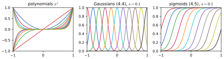
fig_4_2. Reproduces Bishop and Bishop (2024), Figure 4.2. Download: PDF · SVGResult 4.1 (sigmoid and tanh features span the same functions; Exercise 4.3) p. 113, (4.55)–(4.58)
\(\tanh(a)=2\sigma(2a)-1\). Consequently every function \(w_0+\sum_{j=1}^Mw_j\sigma\big((x-\mu_j)/s\big)\) can be written as \(u_0+\sum_{j=1}^Mu_j\tanh\big((x-\mu_j)/2s\big)\) with
\[ u_j=\tfrac12w_j\ (j\ge1),\qquad u_0=w_0+\tfrac12\sum_{j=1}^Mw_j, \]and conversely (\(w_j=2u_j\), \(w_0=u_0-\sum_ju_j\)): the two families define the same set of functions, through an invertible linear map between the parameters.
Proof
Multiply numerator and denominator of \(\tanh a=(e^a-e^{-a})/(e^a+e^{-a})\) by \(e^{-a}\): \(\tanh a=(1-e^{-2a})/(1+e^{-2a})\). On the other hand
\[ 2\sigma(2a)-1=\frac{2}{1+e^{-2a}}-\frac{1+e^{-2a}}{1+e^{-2a}}=\frac{1-e^{-2a}}{1+e^{-2a}}. \]Rearranged, \(\sigma(b)=\tfrac12\{1+\tanh(b/2)\}\). With \(b=(x-\mu_j)/s\), each term \(w_j\sigma(b)=\tfrac12w_j+\tfrac12w_j\tanh\big((x-\mu_j)/2s\big)\); summing over \(j\) and collecting the constants gives the stated \(u_0,u_j\). The map \((w_0,\dots,w_M)\mapsto(u_0,\dots,u_M)\) is linear and triangular with nonzero diagonal, hence invertible, with the inverse given. ∎
The book remarks that the normalisation of a Gaussian basis function is unimportant. That is exactly true for maximum likelihood but not once a penalty is added:
Filling the gap 4.1: rescaling the basis functions p. 113
Replace each \(\phi_j\) by \(c_j\phi_j\) with \(c_j\ne0\), i.e. \(\bPhi\) by \(\bPhi\mathbf{C}\), \(\mathbf{C}=\diag(c_j)\). Is the fitted function the same?
Derivation
Maximum likelihood: yes. The columns of \(\bPhi\mathbf{C}\) span the same subspace as those of \(\bPhi\), and the least-squares fitted vector is the orthogonal projection of \(\mathbf{t}\) onto that subspace (Result 4.5), so the fitted values, and the fitted function \(y(\mathbf{x})=\mathbf{v}^\T\mathbf{C}\bphi(\mathbf{x})\), are unchanged; only the weights change, \(\mathbf{v}=\mathbf{C}^{-1}\mathbf{w}\).
Regularised least squares: no. Minimising \(\tfrac12\|\mathbf{t}-\bPhi\mathbf{C}\mathbf{v}\|^2+\tfrac\lambda2\|\mathbf{v}\|^2\) over \(\mathbf{v}\) is the same, with \(\mathbf{w}=\mathbf{C}\mathbf{v}\), as minimising \(\tfrac12\|\mathbf{t}-\bPhi\mathbf{w}\|^2+\tfrac\lambda2\sum_jw_j^2/c_j^2\): a basis function made larger (\(|c_j|\) big) is penalised less. So with a penalty the scale of each feature matters, which is one reason to standardise features before fitting. ∎
Other bases mentioned in the book are the Fourier basis (each function a single frequency, infinite spatial extent) and wavelets, which are localised in both space and frequency and are usually chosen mutually orthogonal. Most results below hold for any choice of \(\bphi\).
See also (companion course): Filling the gap 5.2 (the same sigmoid/tanh equivalence for hidden units).
4.1.2 Likelihood function
pp. 114–115 Assume the target is a deterministic function plus Gaussian noise of variance \(\sigma^2\):
\[ t=y(\mathbf{x},\mathbf{w})+\epsilon, \tag{4.7} \] \[ p(t\given\mathbf{x},\mathbf{w},\sigma^2)=\N(t\given y(\mathbf{x},\mathbf{w}),\sigma^2). \tag{4.8} \]For independent observations (the column vector \(\mathbf{t}\) of targets, inputs \(\mathbf{X}=\{\mathbf{x}_1,\dots,\mathbf{x}_N\}\)) the likelihood and its logarithm are
\[ p(\mathbf{t}\given\mathbf{X},\mathbf{w},\sigma^2)=\prod_{n=1}^N\N(t_n\given\mathbf{w}^\T\bphi(\mathbf{x}_n),\sigma^2) \tag{4.9} \] \[ \ln p(\mathbf{t}\given\mathbf{X},\mathbf{w},\sigma^2)=-\frac N2\ln\sigma^2-\frac N2\ln(2\pi)-\frac1{\sigma^2}E_D(\mathbf{w}), \tag{4.10} \] \[ E_D(\mathbf{w})=\frac12\sum_{n=1}^N\{t_n-\mathbf{w}^\T\bphi(\mathbf{x}_n)\}^2. \tag{4.11} \]Filling the gap 4.2: from (4.9) to (4.10), and why the noise level does not affect \(\mathbf{w}_{\rm ML}\) p. 115
Derivation
The univariate Gaussian has \(\ln\N(t\given\mu,\sigma^2)=-\tfrac12\ln(2\pi)-\tfrac12\ln\sigma^2-(t-\mu)^2/(2\sigma^2)\). Independence turns the product (4.9) into a sum of \(N\) such terms with \(\mu_n=\mathbf{w}^\T\bphi_n\); the constants add up to \(-\tfrac N2\ln(2\pi)-\tfrac N2\ln\sigma^2\) and the quadratic terms to \(-\sigma^{-2}\cdot\tfrac12\sum_n(t_n-\mu_n)^2=-E_D(\mathbf{w})/\sigma^2\), which is (4.10).
For every fixed \(\sigma^2>0\), (4.10) is a decreasing affine function of \(E_D(\mathbf{w})\), so its maximisers over \(\mathbf{w}\) are exactly the minimisers of \(E_D\), whatever \(\sigma^2\) is. The joint maximisation over \((\mathbf{w},\sigma^2)\) therefore decouples: first minimise \(E_D\) to get \(\mathbf{w}_{\rm ML}\), then maximise over \(\sigma^2\) with \(\mathbf{w}=\mathbf{w}_{\rm ML}\) plugged in (Result 4.4). ∎
See also (companion course): Section 3.1.1, maximum likelihood and least squares.
4.1.3 Maximum likelihood
pp. 115–116 The book writes the gradient of (4.10) as a row vector,
\[ \nabla_{\mathbf{w}}\ln p(\mathbf{t}\given\mathbf{X},\mathbf{w},\sigma^2)=\frac1{\sigma^2}\sum_{n=1}^N\big\{t_n-\mathbf{w}^\T\bphi(\mathbf{x}_n)\big\}\bphi(\mathbf{x}_n)^\T, \tag{4.12} \]sets it to zero,
\[ 0=\sum_{n=1}^Nt_n\bphi(\mathbf{x}_n)^\T-\mathbf{w}^\T\Big(\sum_{n=1}^N\bphi(\mathbf{x}_n)\bphi(\mathbf{x}_n)^\T\Big), \tag{4.13} \]and solves:
\[ \mathbf{w}_{\rm ML}=\big(\bPhi^\T\bPhi\big)^{-1}\bPhi^\T\mathbf{t}. \tag{4.14} \](4.12) is the transpose of the column gradient used everywhere else, including the update (4.21); below we use the column form \(\nabla E_D(\mathbf{w})=-\bPhi^\T(\mathbf{t}-\bPhi\mathbf{w})\).
Definition 4.2 (design matrix and pseudo-inverse) p. 116, (4.15)–(4.16)
The design matrix is the \(N\times M\) matrix \(\Phi_{nj}=\phi_j(\mathbf{x}_n)\):
\[ \bPhi=\begin{pmatrix}\phi_0(\mathbf{x}_1)&\phi_1(\mathbf{x}_1)&\cdots&\phi_{M-1}(\mathbf{x}_1)\\ \phi_0(\mathbf{x}_2)&\phi_1(\mathbf{x}_2)&\cdots&\phi_{M-1}(\mathbf{x}_2)\\ \vdots&\vdots&\ddots&\vdots\\ \phi_0(\mathbf{x}_N)&\phi_1(\mathbf{x}_N)&\cdots&\phi_{M-1}(\mathbf{x}_N)\end{pmatrix}. \tag{4.15} \]Row \(n\) is \(\bphi_n^\T\); column \(j\) is the vector \(\bvphi_j\in\R^N\) of values of \(\phi_j\) at the data. When \(\bPhi\) has full column rank \(M\), its Moore–Penrose pseudo-inverse is
\[ \bPhi^\dagger\equiv\big(\bPhi^\T\bPhi\big)^{-1}\bPhi^\T. \tag{4.16} \]For a general \(\bPhi\) with thin SVD \(\bPhi=\sum_{i=1}^rd_i\mathbf{u}_i\mathbf{v}_i^\T\) (\(r=\rank\bPhi\), \(d_i>0\), orthonormal \(\mathbf{u}_i\in\R^N\), \(\mathbf{v}_i\in\R^M\)) it is \(\bPhi^\dagger=\sum_{i=1}^rd_i^{-1}\mathbf{v}_i\mathbf{u}_i^\T\).
Result 4.2 (the normal equations) pp. 115–116, (4.12)–(4.14)
\(E_D\) is a convex quadratic with gradient and Hessian
\[ \frac{\partial E_D}{\partial w_k}=-\sum_{n=1}^N\Big(t_n-\sum_{j=0}^{M-1}w_j\phi_j(\mathbf{x}_n)\Big)\phi_k(\mathbf{x}_n),\qquad \nabla E_D=\bPhi^\T\bPhi\,\mathbf{w}-\bPhi^\T\mathbf{t},\qquad \nabla\nabla E_D=\bPhi^\T\bPhi. \]Its minimisers are the solutions of the normal equations \(\bPhi^\T\bPhi\,\mathbf{w}=\bPhi^\T\mathbf{t}\). If \(\bPhi\) has full column rank (which needs \(N\ge M\)), the minimiser is unique and equals (4.14). Otherwise the minimisers form the affine set \(\bPhi^\dagger\mathbf{t}+\ker\bPhi\), all with the same fitted values \(\bPhi\mathbf{w}\).
Proof
Expand \(E_D(\mathbf{w})=\tfrac12\|\mathbf{t}-\bPhi\mathbf{w}\|^2=\tfrac12\mathbf{t}^\T\mathbf{t}-\mathbf{w}^\T\bPhi^\T\mathbf{t}+\tfrac12\mathbf{w}^\T\bPhi^\T\bPhi\mathbf{w}\). Using \(\nabla(\mathbf{a}^\T\mathbf{w})=\mathbf{a}\) and \(\nabla(\mathbf{w}^\T\mathbf{A}\mathbf{w})=2\mathbf{A}\mathbf{w}\) for symmetric \(\mathbf{A}\) gives the gradient; the index form is the \(k\)th component, since \((\bPhi^\T\mathbf{r})_k=\sum_n\phi_k(\mathbf{x}_n)r_n\). Differentiating once more gives the Hessian \(\bPhi^\T\bPhi\), which is positive semidefinite: \(\mathbf{v}^\T\bPhi^\T\bPhi\mathbf{v}=\|\bPhi\mathbf{v}\|^2\ge0\).
More directly, for any \(\mathbf{w}^\star\) solving the normal equations and any \(\mathbf{v}\), the exact expansion
\[ E_D(\mathbf{w}^\star+\mathbf{v})=E_D(\mathbf{w}^\star)-\mathbf{v}^\T\bPhi^\T(\mathbf{t}-\bPhi\mathbf{w}^\star)+\tfrac12\|\bPhi\mathbf{v}\|^2=E_D(\mathbf{w}^\star)+\tfrac12\|\bPhi\mathbf{v}\|^2 \]shows that \(\mathbf{w}^\star\) is a global minimiser, and that \(\mathbf{w}^\star+\mathbf{v}\) is another one iff \(\bPhi\mathbf{v}=\mathbf{0}\). Conversely a minimiser has zero gradient, so it solves the normal equations. A solution exists in all cases: \(\bPhi^\dagger\mathbf{t}\) is one (Result 4.3(d)). If \(\bPhi\) has full column rank, \(\ker\bPhi=\{\mathbf{0}\}\), \(\bPhi^\T\bPhi\) is positive definite and hence invertible, and the unique minimiser is (4.14). Transposing (4.13) gives \(\bPhi^\T\mathbf{t}=\bPhi^\T\bPhi\mathbf{w}\), because \(\sum_n\bphi_n\bphi_n^\T=\bPhi^\T\bPhi\) and \(\sum_nt_n\bphi_n=\bPhi^\T\mathbf{t}\). ∎
Result 4.3 (properties of the pseudo-inverse) p. 116
(a) If \(\bPhi\) has full column rank, the SVD formula of Definition 4.2 equals (4.16). (b) If \(\bPhi\) is square and invertible, \(\bPhi^\dagger=\bPhi^{-1}\). (c) Always: \(\bPhi\bPhi^\dagger\bPhi=\bPhi\), \(\bPhi^\dagger\bPhi\bPhi^\dagger=\bPhi^\dagger\), and \(\bPhi\bPhi^\dagger\), \(\bPhi^\dagger\bPhi\) are symmetric (the Penrose conditions, which characterise \(\bPhi^\dagger\) uniquely). (d) \(\bPhi^\dagger\mathbf{t}\) is the least-squares solution of smallest norm. (e) \(\lim_{\lambda\to0^+}(\lambda\mathbf{I}+\bPhi^\T\bPhi)^{-1}\bPhi^\T=\bPhi^\dagger\), with or without full rank.
Proof
Complete \(\{\mathbf{v}_i\}_{i\le r}\) to an orthonormal basis of \(\R^M\) and write \(\mathbf{V}_r,\mathbf{U}_r,\mathbf{D}_r\) for the thin factors, so \(\bPhi=\mathbf{U}_r\mathbf{D}_r\mathbf{V}_r^\T\), \(\bPhi^\dagger=\mathbf{V}_r\mathbf{D}_r^{-1}\mathbf{U}_r^\T\), \(\mathbf{U}_r^\T\mathbf{U}_r=\mathbf{V}_r^\T\mathbf{V}_r=\mathbf{I}_r\).
(a) Full column rank means \(r=M\), so \(\mathbf{V}=\mathbf{V}_r\) is square orthogonal and \(\bPhi^\T\bPhi=\mathbf{V}\mathbf{D}^2\mathbf{V}^\T\). Then \((\bPhi^\T\bPhi)^{-1}\bPhi^\T=\mathbf{V}\mathbf{D}^{-2}\mathbf{V}^\T\mathbf{V}\mathbf{D}\mathbf{U}^\T=\mathbf{V}\mathbf{D}^{-1}\mathbf{U}^\T\).
(b) A square invertible \(\bPhi\) has full column rank, and with \((\mathbf{A}\mathbf{B})^{-1}=\mathbf{B}^{-1}\mathbf{A}^{-1}\): \((\bPhi^\T\bPhi)^{-1}\bPhi^\T=\bPhi^{-1}(\bPhi^\T)^{-1}\bPhi^\T=\bPhi^{-1}\).
(c) \(\bPhi\bPhi^\dagger=\mathbf{U}_r\mathbf{D}_r\mathbf{V}_r^\T\mathbf{V}_r\mathbf{D}_r^{-1}\mathbf{U}_r^\T=\mathbf{U}_r\mathbf{U}_r^\T\) and \(\bPhi^\dagger\bPhi=\mathbf{V}_r\mathbf{V}_r^\T\) are symmetric; then \(\bPhi\bPhi^\dagger\bPhi=\mathbf{U}_r\mathbf{U}_r^\T\mathbf{U}_r\mathbf{D}_r\mathbf{V}_r^\T=\bPhi\) and similarly \(\bPhi^\dagger\bPhi\bPhi^\dagger=\bPhi^\dagger\). (Uniqueness is Penrose's theorem; we do not need it.)
(d) Write any \(\mathbf{w}=\mathbf{V}_r\mathbf{a}+\mathbf{V}_\perp\mathbf{b}\). Since \(\bPhi\mathbf{V}_\perp=\mathbf{0}\) and \(\mathbf{t}=\mathbf{U}_r\mathbf{U}_r^\T\mathbf{t}+(\mathbf{I}-\mathbf{U}_r\mathbf{U}_r^\T)\mathbf{t}\) splits into orthogonal parts, \(\|\mathbf{t}-\bPhi\mathbf{w}\|^2=\|\mathbf{U}_r^\T\mathbf{t}-\mathbf{D}_r\mathbf{a}\|^2+\|(\mathbf{I}-\mathbf{U}_r\mathbf{U}_r^\T)\mathbf{t}\|^2\). The minimum is attained iff \(\mathbf{a}=\mathbf{D}_r^{-1}\mathbf{U}_r^\T\mathbf{t}\), for any \(\mathbf{b}\); and \(\|\mathbf{w}\|^2=\|\mathbf{a}\|^2+\|\mathbf{b}\|^2\) is smallest at \(\mathbf{b}=\mathbf{0}\), i.e. at \(\mathbf{w}=\bPhi^\dagger\mathbf{t}\).
(e) With the full SVD (singular values \(d_i=0\) for \(i>r\)), \((\lambda\mathbf{I}+\bPhi^\T\bPhi)^{-1}\bPhi^\T=\sum_i\frac{d_i}{d_i^2+\lambda}\mathbf{v}_i\mathbf{u}_i^\T\). Each factor tends to \(1/d_i\) if \(d_i>0\) and is identically 0 if \(d_i=0\), which is the SVD formula for \(\bPhi^\dagger\). ∎
The bias parameter. Making \(w_0\) explicit, the error is
\[ E_D(\mathbf{w})=\frac12\sum_{n=1}^N\Big\{t_n-w_0-\sum_{j=1}^{M-1}w_j\phi_j(\mathbf{x}_n)\Big\}^2, \tag{4.17} \]and its stationarity in \(w_0\) gives
\[ w_0=\overline{t}-\sum_{j=1}^{M-1}w_j\overline{\phi_j}, \tag{4.18} \] \[ \overline{t}=\frac1N\sum_{n=1}^Nt_n,\qquad \overline{\phi_j}=\frac1N\sum_{n=1}^N\phi_j(\mathbf{x}_n). \tag{4.19} \]Filling the gap 4.3: the bias absorbs the means p. 116
Derivation, and what it implies
\(\partial E_D/\partial w_0=-\sum_n\{t_n-w_0-\sum_{j\ge1}w_j\phi_j(\mathbf{x}_n)\}=-N\overline{t}+Nw_0+N\sum_{j\ge1}w_j\overline{\phi_j}\); setting it to zero gives (4.18). Because \(E_D\) is convex, (4.18) holds at every minimiser, and substituting it back,
\[ E_D=\frac12\sum_{n=1}^N\Big\{(t_n-\overline{t})-\sum_{j=1}^{M-1}w_j\big(\phi_j(\mathbf{x}_n)-\overline{\phi_j}\big)\Big\}^2 . \]So the non-bias weights are the least-squares fit of the centred targets on the centred features, and the bias then restores the means. Two consequences: (i) adding a constant to every target changes only \(w_0\); (ii) if the features are centred, \(\overline{\phi_j}=0\), the bias column is orthogonal to the others, \(\bPhi^\T\bPhi\) becomes block diagonal and its condition number usually drops, which is why centring speeds up gradient methods (LMS demo, "standardise the input"). The demo readout checks (4.18) at the fitted weights. ∎
Maximising (4.10) over \(\sigma^2\) gives the residual variance
\[ \sigma^2_{\rm ML}=\frac1N\sum_{n=1}^N\{t_n-\mathbf{w}_{\rm ML}^\T\bphi(\mathbf{x}_n)\}^2. \tag{4.20} \]Result 4.4 (the noise variance and its bias) p. 116, (4.20)
If \(E_D(\mathbf{w}_{\rm ML})>0\), (4.20) is the unique maximiser of (4.10) over \(\sigma^2>0\). If the data come from the model, \(\mathbf{t}=\bPhi\mathbf{w}^\star+\bm\epsilon\) with \(\bm\epsilon\sim\N(\mathbf{0},\sigma^2\mathbf{I})\) and \(\bPhi\) of full column rank, then
\[ \E[\sigma^2_{\rm ML}]=\frac{N-M}{N}\,\sigma^2, \]so \(\sigma^2_{\rm ML}\) underestimates the noise, and \(\frac{1}{N-M}\sum_n\{t_n-\mathbf{w}_{\rm ML}^\T\bphi_n\}^2\) is unbiased.
Proof
With \(E=E_D(\mathbf{w}_{\rm ML})\) and \(v=\sigma^2\), \(g(v)=-\tfrac N2\ln v-E/v\) (plus a constant) has \(g'(v)=-\tfrac N{2v}+\tfrac E{v^2}\), which is positive for \(v\lt 2E/N\) and negative after, so \(v=2E/N\) (that is (4.20)) is the unique maximiser.
For the bias, let \(\mathbf{P}=\bPhi(\bPhi^\T\bPhi)^{-1}\bPhi^\T\) (Result 4.5). The residual vector is \(\mathbf{t}-\bPhi\mathbf{w}_{\rm ML}=(\mathbf{I}-\mathbf{P})\mathbf{t}=(\mathbf{I}-\mathbf{P})\bm\epsilon\), because \((\mathbf{I}-\mathbf{P})\bPhi=\mathbf{0}\). With \(\mathbf{I}-\mathbf{P}\) symmetric and idempotent,
\[ \E\|(\mathbf{I}-\mathbf{P})\bm\epsilon\|^2=\E\,\bm\epsilon^\T(\mathbf{I}-\mathbf{P})\bm\epsilon=\Tr\big((\mathbf{I}-\mathbf{P})\E[\bm\epsilon\bm\epsilon^\T]\big)=\sigma^2\Tr(\mathbf{I}-\mathbf{P})=\sigma^2(N-M), \]using \(\Tr\mathbf{P}=\Tr\big((\bPhi^\T\bPhi)^{-1}\bPhi^\T\bPhi\big)=\Tr\mathbf{I}_M=M\). Divide by \(N\). Fitting \(M\) parameters uses up \(M\) of the \(N\) dimensions in which the noise lives; this is the regression version of the \(N/(N-1)\) correction for the variance of a Gaussian (Chapter 2 of the book). Checked by simulation. ∎
See also (companion course): Result 3.1 (normal equations), Filling the gap 3.1 (the bias parameter), Result 3.2 (the noise precision).
4.1.4 Geometry of least squares
pp. 116–117 View \(\mathbf{t}\) as a point of \(\R^N\) and each column \(\bvphi_j\) of \(\bPhi\) as a vector of \(\R^N\). The fitted vector \(\mathbf{y}=\bPhi\mathbf{w}\) (with \(y_n=y(\mathbf{x}_n,\mathbf{w})\)) ranges over the span \(\mathcal{S}\) of the columns, a subspace of dimension \(\rank\bPhi\) (which is \(M\) when the columns are linearly independent, the case the book has in mind). Since \(E_D=\tfrac12\|\mathbf{t}-\mathbf{y}\|^2\), least squares picks the point of \(\mathcal{S}\) closest to \(\mathbf{t}\).
Result 4.5 (least squares is an orthogonal projection; Exercise 4.4) p. 117, (4.59)
Let \(\bPhi\) have full column rank and \(\mathbf{P}=\bPhi(\bPhi^\T\bPhi)^{-1}\bPhi^\T\) (4.59). Then (i) \(\mathbf{P}^\T=\mathbf{P}\) and \(\mathbf{P}^2=\mathbf{P}\); (ii) \(\mathbf{P}\mathbf{v}\in\mathcal{S}\) for every \(\mathbf{v}\), and \(\mathbf{P}\mathbf{s}=\mathbf{s}\) for \(\mathbf{s}\in\mathcal{S}\); (iii) \(\mathbf{v}-\mathbf{P}\mathbf{v}\perp\mathcal{S}\); (iv) \(\|\mathbf{v}-\mathbf{s}\|^2=\|\mathbf{v}-\mathbf{P}\mathbf{v}\|^2+\|\mathbf{P}\mathbf{v}-\mathbf{s}\|^2\) for \(\mathbf{s}\in\mathcal{S}\), so \(\mathbf{P}\mathbf{v}\) is the unique closest point of \(\mathcal{S}\). In particular \(\mathbf{y}=\bPhi\mathbf{w}_{\rm ML}=\mathbf{P}\mathbf{t}\) is the orthogonal projection of \(\mathbf{t}\) onto \(\mathcal{S}\). Without full rank the same holds with \(\mathbf{P}=\bPhi\bPhi^\dagger\).
Proof
(i) \(\mathbf{P}^\T=\bPhi(\bPhi^\T\bPhi)^{-\T}\bPhi^\T=\mathbf{P}\) because \(\bPhi^\T\bPhi\) is symmetric; \(\mathbf{P}^2=\bPhi(\bPhi^\T\bPhi)^{-1}(\bPhi^\T\bPhi)(\bPhi^\T\bPhi)^{-1}\bPhi^\T=\mathbf{P}\). (ii) \(\mathbf{P}\mathbf{v}=\bPhi\tilde{\mathbf{v}}\) with \(\tilde{\mathbf{v}}=(\bPhi^\T\bPhi)^{-1}\bPhi^\T\mathbf{v}\), a combination \(\sum_j\tilde v_j\bvphi_j\) of the columns. Each column is fixed: \(\mathbf{P}\bvphi_j\) is column \(j\) of \(\mathbf{P}\bPhi=\bPhi\), so by linearity \(\mathbf{P}\mathbf{s}=\mathbf{s}\) on \(\mathcal{S}\). (iii) For every column, \(\bvphi_j^\T(\mathbf{v}-\mathbf{P}\mathbf{v})=\big(\bPhi^\T(\mathbf{I}-\mathbf{P})\mathbf{v}\big)_j=0\), since \(\bPhi^\T\mathbf{P}=\bPhi^\T\); hence \(\mathbf{v}-\mathbf{P}\mathbf{v}\) is orthogonal to all of \(\mathcal{S}\). (iv) \(\mathbf{v}-\mathbf{s}=(\mathbf{v}-\mathbf{P}\mathbf{v})+(\mathbf{P}\mathbf{v}-\mathbf{s})\) with the second vector in \(\mathcal{S}\), orthogonal to the first by (iii): Pythagoras. The second term is zero only for \(\mathbf{s}=\mathbf{P}\mathbf{v}\). Finally \(\bPhi\mathbf{w}_{\rm ML}=\bPhi(\bPhi^\T\bPhi)^{-1}\bPhi^\T\mathbf{t}=\mathbf{P}\mathbf{t}\). Without full rank, \(\bPhi\bPhi^\dagger=\mathbf{U}_r\mathbf{U}_r^\T\) is symmetric idempotent with range \(\mathcal{S}\) (Result 4.3(c)), and the same argument applies. ∎
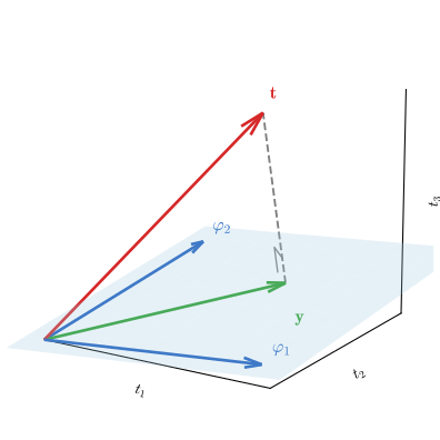
fig_4_3. Reproduces Bishop and Bishop (2024), Figure 4.3. Download: PDF · SVGThe book warns that solving the normal equations directly is numerically delicate when \(\bPhi^\T\bPhi\) is close to singular, recommends the SVD, and notes that a regulariser makes the matrix non-singular. Here is why.
Filling the gap 4.4: conditioning, the SVD, and why a penalty helps p. 117
Derivation
Squared condition number. The singular values of \(\bPhi^\T\bPhi=\mathbf{V}\mathbf{D}^2\mathbf{V}^\T\) are \(d_i^2\), so \(\kappa(\bPhi^\T\bPhi)=d_{\max}^2/d_{\min}^2=\kappa(\bPhi)^2\). A linear solve with condition number \(\kappa\) in double precision (unit roundoff \(u\approx1.1\times10^{-16}\)) can lose about \(\log_{10}\kappa\) digits. Forming \(\bPhi^\T\bPhi\) and solving therefore gives errors of order \(\kappa(\bPhi)^2u\), while methods that work with \(\bPhi\) itself (QR or the SVD) have errors of order \(\kappa(\bPhi)u\) for problems with small residuals (Golub and Van Loan, 1996, Chapter 5). Once \(\kappa(\bPhi)>u^{-1/2}\approx10^8\), the normal equations can return no correct digits at all.
Near-collinear columns give huge weights. If two columns are almost equal, \(\bvphi_j\approx\bvphi_k\), then \(\bPhi(\mathbf{e}_j-\mathbf{e}_k)\approx\mathbf{0}\): a direction with a tiny singular value \(d_{\min}\). Along it, the least-squares solution \(\sum_i d_i^{-1}(\mathbf{u}_i^\T\mathbf{t})\mathbf{v}_i\) has a component of size \(|\mathbf{u}_{\min}^\T\mathbf{t}|/d_{\min}\): the two weights become large and of opposite sign, cancelling in the fit. Small changes in \(\mathbf{t}\) move them wildly.
Truncated SVD. Treating singular values below \(\varepsilon d_{\max}\) as zero (\(\varepsilon=10^{-12}\) in our code and demo) returns the minimum-norm solution of the nearby rank-deficient problem (Result 4.3(d)), which is stable, though the kept small \(d_i\) can still produce large weights.
The penalty. \(\lambda\mathbf{I}+\bPhi^\T\bPhi\) has eigenvalues \(\lambda+d_i^2\ge\lambda>0\): it is invertible for every \(\bPhi\), with condition number at most \((d_{\max}^2+\lambda)/\lambda\). In the SVD form of Result 4.7 each coefficient \(d_i/(d_i^2+\lambda)\le1/(2\sqrt\lambda)\) (because \(d_i^2+\lambda\ge2d_i\sqrt\lambda\)), so \(\|\mathbf{w}_\lambda\|\le\|\mathbf{t}\|/(2\sqrt\lambda)\) whatever the degeneracy.
Numbers. With 24 Gaussian basis functions of width \(s=0.4\) on 25 points (demo preset 4), \(\kappa(\bPhi)\approx10^{18}\): \(\bPhi^\T\bPhi\) is numerically singular. Perturbing \(\mathbf{t}\) by \(10^{-9}\) changes the direct normal-equation solution by a relative \(4\times10^{-6}\) and the truncated-SVD solution by \(2\times10^{-9}\). ∎
See also (companion course): Section 3.1.2, geometry of least squares, and Filling the gap 3.2 (the SVD and numerical trouble).
4.1.5 Sequential learning
pp. 117–118 The solution (4.14) is a batch method: it uses the whole data set at once. For large data sets, or for data arriving as a stream, a sequential (on-line) algorithm updates the weights after each data point. If the error is a sum \(E=\sum_nE_n\), stochastic gradient descent updates
\[ \mathbf{w}^{(\tau+1)}=\mathbf{w}^{(\tau)}-\eta\nabla E_n, \tag{4.21} \]with learning rate \(\eta>0\) and iteration counter \(\tau\), starting from some \(\mathbf{w}^{(0)}\).
Algorithm 4.1 (least-mean-squares, LMS) p. 118, (4.22)
- Choose \(\mathbf{w}^{(0)}\) (e.g. \(\mathbf{0}\)) and a learning rate \(\eta\) (or a schedule \(\eta_\tau\)).
- For \(\tau=0,1,2,\dots\): pick a data point \(n\) (cyclically, or at random), compute the residual \(r=t_n-\mathbf{w}^{(\tau)\T}\bphi_n\) and update \[ \mathbf{w}^{(\tau+1)}=\mathbf{w}^{(\tau)}+\eta\big(t_n-\mathbf{w}^{(\tau)\T}\bphi_n\big)\bphi_n. \tag{4.22} \]
Cost: \(O(M)\) per update, against \(O(NM^2+M^3)\) for the batch solution.
The book gives the update and moves on (stochastic gradient descent is treated in Chapter 7). How it actually behaves is easy to work out for this quadratic error, and the answer explains the familiar rules of thumb: a learning rate that is too large diverges, a constant one never quite converges on noisy data, and a decreasing one does.
Result 4.6 (what LMS does) pp. 117–118
Let \(\mathbf{A}=\bPhi^\T\bPhi\) have full rank, with eigenvalues \(0\lt \lambda_{\min}\le\dots\le\lambda_{\max}\).
(a) One step. \(\nabla E_n(\mathbf{w})=-(t_n-\mathbf{w}^\T\bphi_n)\bphi_n\), so (4.21) is (4.22), and the update multiplies the residual on the presented point by \(1-\eta\|\bphi_n\|^2\). It reduces that residual iff \(0\lt \eta\lt 2/\|\bphi_n\|^2\), and \(\eta=1/\|\bphi_n\|^2\) fits the point exactly.
(b) Batch gradient descent \(\mathbf{w}\leftarrow\mathbf{w}-\eta\nabla E_D\) converges to \(\mathbf{w}_{\rm ML}\) from every start iff \(0\lt \eta\lt 2/\lambda_{\max}\), linearly with rate \(\max(|1-\eta\lambda_{\min}|,|1-\eta\lambda_{\max}|)\); the best fixed rate \(\eta=2/(\lambda_{\max}+\lambda_{\min})\) gives \((\kappa-1)/(\kappa+1)\) with \(\kappa=\lambda_{\max}/\lambda_{\min}\).
(c) Consistent data. If some \(\mathbf{w}^\star\) fits every point exactly (\(t_n=\mathbf{w}^{\star\T}\bphi_n\) for all \(n\)) and \(0\lt \eta\|\bphi_n\|^2\lt 2\) for all \(n\), cyclic LMS with constant \(\eta\) converges to \(\mathbf{w}^\star=\mathbf{w}_{\rm ML}\) geometrically (this is the Kaczmarz method).
(d) Noisy data, constant \(\eta\). If some residual \(r_n=t_n-\mathbf{w}_{\rm ML}^\T\bphi_n\) is nonzero, \(\mathbf{w}_{\rm ML}\) is not a fixed point of an LMS epoch. Under the conditions of (c), the cyclic iterates converge to a cycle of \(N\) points, all at distance \(O(\eta)\) from \(\mathbf{w}_{\rm ML}\) as \(\eta\to0\), but not at \(\mathbf{w}_{\rm ML}\).
(e) Decreasing \(\eta_\tau\). With \(\sum_\tau\eta_\tau=\infty\) and \(\sum_\tau\eta_\tau^2\lt \infty\) (e.g. \(\eta_\tau=\eta/(1+\tau/N)\)), LMS converges to \(\mathbf{w}_{\rm ML}\) (Robbins and Monro, 1951, for randomly sampled points; see Chapter 7 of the book).
Proof of (a)–(d), and the idea behind (e)
(a) \(E_n=\tfrac12(t_n-\mathbf{w}^\T\bphi_n)^2\) has gradient \(-(t_n-\mathbf{w}^\T\bphi_n)\bphi_n\) by the chain rule, giving (4.22). After the step, \(t_n-\mathbf{w}'^\T\bphi_n=r-\eta r\bphi_n^\T\bphi_n=(1-\eta\|\bphi_n\|^2)r\); the factor has modulus below 1 iff \(0\lt \eta\|\bphi_n\|^2\lt 2\), and vanishes at \(\eta=1/\|\bphi_n\|^2\), when \(\mathbf{w}'\) is the projection of \(\mathbf{w}\) onto the hyperplane \(\{\mathbf{v}:\mathbf{v}^\T\bphi_n=t_n\}\).
(b) With \(\mathbf{e}=\mathbf{w}-\mathbf{w}_{\rm ML}\) and \(\nabla E_D=\mathbf{A}\mathbf{w}-\bPhi^\T\mathbf{t}=\mathbf{A}\mathbf{e}\) (normal equations), the step is \(\mathbf{e}'=(\mathbf{I}-\eta\mathbf{A})\mathbf{e}\). In the eigenbasis of \(\mathbf{A}\) each component is multiplied by \(1-\eta\lambda_i\) per step, so \(\mathbf{e}\to\mathbf{0}\) for every start iff \(|1-\eta\lambda_i|\lt 1\) for all \(i\), i.e. \(0\lt \eta\lt 2/\lambda_{\max}\), and the slowest component decays at the stated rate. The rate is minimised when \(1-\eta\lambda_{\min}=-(1-\eta\lambda_{\max})\), i.e. \(\eta=2/(\lambda_{\min}+\lambda_{\max})\), giving \((\lambda_{\max}-\lambda_{\min})/(\lambda_{\max}+\lambda_{\min})\).
(c) Now \(r=(\mathbf{w}^\star-\mathbf{w})^\T\bphi_n\), so \(\mathbf{e}=\mathbf{w}-\mathbf{w}^\star\) obeys \(\mathbf{e}'=(\mathbf{I}-\eta\bphi_n\bphi_n^\T)\mathbf{e}\) and
\[ \|\mathbf{e}'\|^2=\|\mathbf{e}\|^2-\eta\big(2-\eta\|\bphi_n\|^2\big)(\bphi_n^\T\mathbf{e})^2\le\|\mathbf{e}\|^2 . \]One epoch is the linear map \(\mathbf{M}=\prod_{n}(\mathbf{I}-\eta\bphi_n\bphi_n^\T)\) (in visiting order). By the display, \(\|\mathbf{M}\mathbf{v}\|\le\|\mathbf{v}\|\), with equality only if \(\bphi_n^\T\mathbf{v}_k=0\) at every step \(k\), where \(\mathbf{v}_k\) is the vector before step \(k\); but then each step leaves the vector unchanged, so \(\mathbf{v}_k=\mathbf{v}\) and \(\bphi_n^\T\mathbf{v}=0\) for all \(n\), i.e. \(\bPhi\mathbf{v}=\mathbf{0}\), so \(\mathbf{v}=\mathbf{0}\) (full rank). The continuous function \(\mathbf{v}\mapsto\|\mathbf{M}\mathbf{v}\|\) on the compact unit sphere therefore has maximum \(\rho=\|\mathbf{M}\|\lt 1\), and after \(k\) epochs \(\|\mathbf{e}\|\le\rho^k\|\mathbf{e}^{(0)}\|\).
(d) An epoch is now affine, \(\mathbf{w}\mapsto\mathbf{M}\mathbf{w}+\mathbf{c}_\eta\) with the same \(\mathbf{M}\). Since \(\|\mathbf{M}\|\lt 1\), it has a unique fixed point \(\mathbf{w}_\eta=(\mathbf{I}-\mathbf{M})^{-1}\mathbf{c}_\eta\) to which the start-of-epoch iterates converge geometrically, and the points visited within the epoch form the limit cycle. Starting an epoch at \(\mathbf{w}_{\rm ML}\), the first step moves by \(\eta r_n\bphi_n\), so \(\mathbf{w}_{\rm ML}\) is not fixed unless every residual is zero along the way. To size the cycle, expand in \(\eta\): \(\mathbf{M}=\mathbf{I}-\eta\mathbf{A}+O(\eta^2)\), and one epoch from \(\mathbf{w}_{\rm ML}\) ends at \(\mathbf{w}_{\rm ML}+\eta\sum_nr_n\bphi_n+O(\eta^2)=\mathbf{w}_{\rm ML}+O(\eta^2)\), because \(\sum_nr_n\bphi_n=\bPhi^\T(\mathbf{t}-\bPhi\mathbf{w}_{\rm ML})=\mathbf{0}\) (normal equations). Thus \(\mathbf{M}\mathbf{w}_{\rm ML}+\mathbf{c}_\eta=\mathbf{w}_{\rm ML}+\bm\delta\) with \(\bm\delta=O(\eta^2)\), and
\[ \mathbf{w}_\eta-\mathbf{w}_{\rm ML}=(\mathbf{I}-\mathbf{M})^{-1}\bm\delta=\big(\eta\mathbf{A}+O(\eta^2)\big)^{-1}O(\eta^2)=O(\eta). \]Points within the cycle differ from \(\mathbf{w}_\eta\) by at most \(N\) steps of size \(O(\eta)\). Numerically, for the demo's data, the distance from \(\mathbf{w}_\eta\) to \(\mathbf{w}_{\rm ML}\) is 0.0715, 0.0377, 0.0190, 0.0095 for \(\eta=0.1,0.05,0.025,0.0125\): it halves with \(\eta\), so it is of order exactly \(\eta\) and not zero.
(e) The idea: the \(O(\eta)\) cycle of (d) shrinks if \(\eta_\tau\to0\); \(\sum\eta_\tau^2\lt \infty\) makes the accumulated noise from the nonzero residuals summable, while \(\sum\eta_\tau=\infty\) keeps enough total step length to reach \(\mathbf{w}_{\rm ML}\) from any start. A full proof for randomly sampled points is the Robbins–Monro theorem (stochastic approximation); a numerical run gives \(\|\mathbf{w}-\mathbf{w}_{\rm ML}\|=2\times10^{-3}\) after 2000 epochs with \(\eta_\tau=0.8/(1+\tau/N)\), cyclic order, and decreasing. ∎
See also (companion course): Section 3.1.3 and Result 3.4 (the LMS update and the batch step-size condition), and the sequential Bayesian regression demo.
4.1.6 Regularized least squares
p. 118 To control over-fitting, add a penalty with regularisation coefficient \(\lambda\ge0\),
\[ E_D(\mathbf{w})+\lambda E_W(\mathbf{w}), \tag{4.23} \] \[ E_W(\mathbf{w})=\frac12\sum_jw_j^2=\frac12\mathbf{w}^\T\mathbf{w}, \tag{4.24} \] \[ E_D(\mathbf{w})=\frac12\sum_{n=1}^N\{t_n-\mathbf{w}^\T\bphi(\mathbf{x}_n)\}^2, \tag{4.25} \] \[ \frac12\sum_{n=1}^N\{t_n-\mathbf{w}^\T\bphi(\mathbf{x}_n)\}^2+\frac\lambda2\mathbf{w}^\T\mathbf{w}. \tag{4.26} \]In statistics this is ridge regression, a shrinkage method (Hoerl and Kennard, 1970); in machine learning, weight decay. Its minimiser is
\[ \mathbf{w}=\big(\lambda\mathbf{I}+\bPhi^\T\bPhi\big)^{-1}\bPhi^\T\mathbf{t}. \tag{4.27} \]Result 4.7 (ridge regression; Exercise 4.6) p. 118, (4.26)–(4.27)
For \(\lambda>0\), (4.26) is strictly convex and (4.27) is its unique minimiser, for every \(\bPhi\) (any rank, any \(N\) and \(M\)). With the SVD \(\bPhi=\sum_id_i\mathbf{u}_i\mathbf{v}_i^\T\),
\[ \mathbf{w}_\lambda=\sum_i\frac{d_i}{d_i^2+\lambda}(\mathbf{u}_i^\T\mathbf{t})\,\mathbf{v}_i,\qquad \bPhi\mathbf{w}_\lambda=\sum_i\frac{d_i^2}{d_i^2+\lambda}(\mathbf{u}_i^\T\mathbf{t})\,\mathbf{u}_i , \]so the component of the fit along \(\mathbf{u}_i\) is the least-squares component multiplied by the shrinkage factor \(d_i^2/(d_i^2+\lambda)\in(0,1)\): directions that the data determine poorly (small \(d_i\)) are shrunk most. Moreover \(\|\mathbf{w}_\lambda\|\) is nonincreasing in \(\lambda\) (strictly decreasing unless \(\bPhi^\T\mathbf{t}=\mathbf{0}\)), \(\bPhi^\T(\mathbf{t}-\bPhi\mathbf{w}_\lambda)=\lambda\mathbf{w}_\lambda\) (the residual is no longer orthogonal to \(\mathcal{S}\)), and the effective number of parameters \(\Tr\big(\bPhi(\lambda\mathbf{I}+\bPhi^\T\bPhi)^{-1}\bPhi^\T\big)=\sum_id_i^2/(d_i^2+\lambda)\) falls from \(\rank\bPhi\) to 0 as \(\lambda\) grows.
Proof
The gradient of (4.26) is \(-\sum_n\{t_n-\mathbf{w}^\T\bphi_n\}\bphi_n+\lambda\mathbf{w}=-\bPhi^\T\mathbf{t}+\bPhi^\T\bPhi\mathbf{w}+\lambda\mathbf{w}\) (Result 4.2 plus \(\nabla\tfrac\lambda2\mathbf{w}^\T\mathbf{w}=\lambda\mathbf{w}\)). Setting it to zero gives \((\lambda\mathbf{I}+\bPhi^\T\bPhi)\mathbf{w}=\bPhi^\T\mathbf{t}\). The Hessian \(\lambda\mathbf{I}+\bPhi^\T\bPhi\) has eigenvalues \(\lambda+d_i^2\ge\lambda>0\) (with \(d_i=0\) for missing directions), so it is positive definite: the error is strictly convex, the matrix is invertible, and (4.27) is the unique global minimiser.
In the basis \(\{\mathbf{v}_i\}\) (completed to all of \(\R^M\)), \(\lambda\mathbf{I}+\bPhi^\T\bPhi=\sum_i(\lambda+d_i^2)\mathbf{v}_i\mathbf{v}_i^\T\) and \(\bPhi^\T\mathbf{t}=\sum_id_i(\mathbf{u}_i^\T\mathbf{t})\mathbf{v}_i\), which gives the SVD form of \(\mathbf{w}_\lambda\); multiplying by \(\bPhi\) (\(\bPhi\mathbf{v}_i=d_i\mathbf{u}_i\)) gives the fitted values. Then \(\|\mathbf{w}_\lambda\|^2=\sum_id_i^2(\mathbf{u}_i^\T\mathbf{t})^2/(d_i^2+\lambda)^2\), each term nonincreasing in \(\lambda\) and strictly decreasing when \(d_i\mathbf{u}_i^\T\mathbf{t}\ne0\). The residual identity is the stationarity condition rearranged. The trace is \(\sum_i d_i^2/(d_i^2+\lambda)\) since the hat matrix is \(\sum_i\frac{d_i^2}{d_i^2+\lambda}\mathbf{u}_i\mathbf{u}_i^\T\); each term decreases from 1 (if \(d_i>0\)) to 0. ∎
Filling the gap 4.5: should the bias be penalised? p. 118
(4.24) sums over all \(j\), and (4.27) uses \(\lambda\mathbf{I}\), so the bias \(w_0\) is penalised too. That makes the fit depend on the origin of the targets.
Derivation
Penalising \(w_0\). If every target is shifted, \(t_n\to t_n+c\), the unpenalised solution changes only by \(w_0\to w_0+c\) (Filling the gap 4.3). With (4.26), shifting \(w_0\) by \(c\) costs \(\tfrac\lambda2\{(w_0+c)^2-w_0^2\}\), so the optimum moves by less than \(c\) and the fitted curve is pulled towards 0: predictions are not shift-equivariant.
Not penalising \(w_0\). Minimise \(E_D(\mathbf{w})+\tfrac\lambda2\sum_{j\ge1}w_j^2\). The derivative in \(w_0\) is the same as without a penalty, so (4.18) still holds; substituting it, as in Filling the gap 4.3, leaves ridge regression of the centred targets on the centred features for \(w_1,\dots,w_{M-1}\). This version is shift-equivariant. When the targets have mean near zero, as for the sinusoid of Figure 4.7, the two versions differ little; the code follows the book and penalises all weights. ∎
See also (companion course): Section 3.1.4, with Result 3.6 (penalised and constrained forms are equivalent) and the lasso.
4.1.7 Multiple outputs
pp. 119–120 For \(K>1\) targets \(\mathbf{t}=(t_1,\dots,t_K)^\T\), use the same basis for every output:
\[ \mathbf{y}(\mathbf{x},\mathbf{w})=\mathbf{W}^\T\bphi(\mathbf{x}), \tag{4.28} \]with \(\mathbf{W}\) of size \(M\times K\): a network with one layer of weights and \(K\) output nodes (Figure 4.4). With isotropic Gaussian noise,
\[ p(\mathbf{t}\given\mathbf{x},\mathbf{W},\sigma^2)=\N(\mathbf{t}\given\mathbf{W}^\T\bphi(\mathbf{x}),\sigma^2\mathbf{I}). \tag{4.29} \]Stacking the targets as the rows of \(\mathbf{T}\in\R^{N\times K}\), the log likelihood is
\[ \ln p(\mathbf{T}\given\mathbf{X},\mathbf{W},\sigma^2)=\sum_{n=1}^N\ln\N(\mathbf{t}_n\given\mathbf{W}^\T\bphi(\mathbf{x}_n),\sigma^2\mathbf{I})=-\frac{NK}2\ln(2\pi\sigma^2)-\frac1{2\sigma^2}\sum_{n=1}^N\big\|\mathbf{t}_n-\mathbf{W}^\T\bphi(\mathbf{x}_n)\big\|^2, \tag{4.30} \]maximised by
\[ \mathbf{W}_{\rm ML}=\big(\bPhi^\T\bPhi\big)^{-1}\bPhi^\T\mathbf{T}, \tag{4.31} \] \[ \mathbf{w}_k=\big(\bPhi^\T\bPhi\big)^{-1}\bPhi^\T\mathbf{t}_k=\bPhi^\dagger\mathbf{t}_k, \tag{4.32} \]where \(\mathbf{t}_k\) is column \(k\) of \(\mathbf{T}\): one pseudo-inverse serves all \(K\) outputs.
Result 4.8 (multiple outputs decouple, for any noise covariance; Exercise 4.7) pp. 119–120, (4.30)–(4.32), (4.61)–(4.63)
(a) (4.30) holds and is maximised by (4.31); column \(k\) is the single-output solution (4.32). (b) If instead \(p(\mathbf{t}\given\mathbf{x})=\N(\mathbf{t}\given\mathbf{W}^\T\bphi(\mathbf{x}),\bm\Sigma)\) with any positive definite \(\bm\Sigma\), the maximum likelihood \(\mathbf{W}\) is still (4.31), whatever \(\bm\Sigma\) is, and the maximum likelihood covariance is
\[ \bm\Sigma_{\rm ML}=\frac1N\sum_{n=1}^N\big(\mathbf{t}_n-\mathbf{W}_{\rm ML}^\T\bphi(\mathbf{x}_n)\big)\big(\mathbf{t}_n-\mathbf{W}_{\rm ML}^\T\bphi(\mathbf{x}_n)\big)^\T. \tag{4.63} \]Proof
(a) \(\ln\N(\mathbf{t}\given\bm\mu,\sigma^2\mathbf{I}_K)=-\tfrac K2\ln(2\pi\sigma^2)-\|\mathbf{t}-\bm\mu\|^2/(2\sigma^2)\) because \(|\sigma^2\mathbf{I}_K|=\sigma^{2K}\); summing over \(n\) gives (4.30). The sum of squares is the squared Frobenius norm \(\|\mathbf{T}-\bPhi\mathbf{W}\|_F^2=\sum_k\|\mathbf{t}_k-\bPhi\mathbf{w}_k\|^2\), a sum of \(K\) single-output errors, each involving only its own column \(\mathbf{w}_k\). Minimising each separately gives (4.32) by Result 4.2, and stacking the columns gives (4.31).
(b) With \(\bm\Lambda=\bm\Sigma^{-1}\) and residual matrix \(\mathbf{E}=\mathbf{T}-\bPhi\mathbf{W}\),
\[ \ln L(\mathbf{W},\bm\Sigma)=-\frac{NK}2\ln2\pi+\frac N2\ln|\bm\Lambda|-\frac12\Tr\big(\mathbf{E}\bm\Lambda\mathbf{E}^\T\big). \]For fixed \(\bm\Lambda\), the gradient in \(\mathbf{W}\) (toolkit: \(\partial\Tr(\mathbf{E}\bm\Lambda\mathbf{E}^\T)/\partial\mathbf{W}=-2\bPhi^\T\mathbf{E}\bm\Lambda\)) is \(\bPhi^\T(\mathbf{T}-\bPhi\mathbf{W})\bm\Lambda\). Since \(\bm\Lambda\) is invertible, it vanishes iff \(\bPhi^\T(\mathbf{T}-\bPhi\mathbf{W})=\mathbf{0}\), the same equations as in (a), and the objective is concave in \(\mathbf{W}\) (its Hessian is \(-\bm\Lambda\otimes\bPhi^\T\bPhi\)). So \(\mathbf{W}_{\rm ML}\) is (4.31) for every \(\bm\Sigma\), and the joint maximisation decouples as in Filling the gap 4.2. With \(\mathbf{W}=\mathbf{W}_{\rm ML}\) and \(\mathbf{S}=\mathbf{E}^\T\mathbf{E}\), maximise \(\tfrac N2\ln|\bm\Lambda|-\tfrac12\Tr(\bm\Lambda\mathbf{S})\) over positive definite \(\bm\Lambda\): the gradient \(\tfrac N2\bm\Lambda^{-1}-\tfrac12\mathbf{S}\) vanishes at \(\bm\Lambda^{-1}=\mathbf{S}/N\), which is (4.63), and the function is concave (\(\ln|\bm\Lambda|\) is concave, the trace linear), so this is the maximum when \(\mathbf{S}\) is positive definite. This is the same argument as for the covariance of a multivariate Gaussian (Chapter 3 of the book): the mean parameters do not depend on the covariance. Checked numerically with a non-isotropic \(\bm\Sigma\). ∎
See also (companion course): Section 3.1.5 and Result 3.7; the matrix derivatives are in the toolkit.
4.2 Decision theory
pp. 120–123 Maximum likelihood gives a predictive distribution,
\[ p(t\given\mathbf{x},\mathbf{w}_{\rm ML},\sigma^2_{\rm ML})=\N(t\given y(\mathbf{x},\mathbf{w}_{\rm ML}),\sigma^2_{\rm ML}), \tag{4.33} \]but an application often needs a single number \(f(\mathbf{x})\), say a radiation dose. The task splits into an inference stage (learn \(p(t\given\mathbf{x})\)) and a decision stage (choose \(f(\mathbf{x})\) to minimise an expected loss \(L(t,f(\mathbf{x}))\)):
\[ \E[L]=\iint L(t,f(\mathbf{x}))\,p(\mathbf{x},t)\d\mathbf{x}\d t. \tag{4.34} \]For the squared loss \(L=\{f(\mathbf{x})-t\}^2\),
\[ \E[L]=\iint\{f(\mathbf{x})-t\}^2p(\mathbf{x},t)\d\mathbf{x}\d t. \tag{4.35} \]The loss must not be confused with the sum-of-squares error function of Section 4.1: the error function is used in training to fit \(p(t\given\mathbf{x})\); the loss is used afterwards to turn the fitted distribution into a prediction. Treating \(f\) as a completely flexible function, the calculus of variations gives
\[ \frac{\delta\E[L]}{\delta f(\mathbf{x})}=2\int\{f(\mathbf{x})-t\}p(\mathbf{x},t)\d t=0, \tag{4.36} \] \[ f^\star(\mathbf{x})=\frac1{p(\mathbf{x})}\int t\,p(\mathbf{x},t)\d t=\int t\,p(t\given\mathbf{x})\d t=\E_t[t\given\mathbf{x}], \tag{4.37} \]the regression function; for the Gaussian model (4.8),
\[ \E[t\given\mathbf{x}]=\int t\,p(t\given\mathbf{x})\d t=y(\mathbf{x},\mathbf{w}). \tag{4.38} \]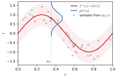
fig_4_5. Reproduces Bishop and Bishop (2024), Figure 4.5. Download: PDF · SVGThe book then expands the square,
\[ \{f(\mathbf{x})-t\}^2=\{f(\mathbf{x})-\E[t\given\mathbf{x}]\}^2+2\{f(\mathbf{x})-\E[t\given\mathbf{x}]\}\{\E[t\given\mathbf{x}]-t\}+\{\E[t\given\mathbf{x}]-t\}^2, \]and states that after integrating over \(t\) the cross term vanishes, leaving
\[ \E[L]=\int\{f(\mathbf{x})-\E[t\given\mathbf{x}]\}^2p(\mathbf{x})\d\mathbf{x}+\int\var[t\given\mathbf{x}]\,p(\mathbf{x})\d\mathbf{x}. \tag{4.39} \]Result 4.9 (the conditional mean minimises the expected squared loss; Exercises 4.8–4.10) pp. 121–122, (4.35)–(4.39), (4.64)–(4.65)
Assume \(\E[t^2]\lt \infty\) and let \(h(\mathbf{x})=\E[t\given\mathbf{x}]\). For every function \(f\) with \(\E[f(\mathbf{x})^2]\lt \infty\), (4.39) holds; hence \(h\) minimises (4.35), the minimum is \(\E[\var(t\given\mathbf{x})]\), and any other minimiser equals \(h\) except on a set of \(\mathbf{x}\) of probability zero. For a vector target \(\mathbf{t}\) and the loss \(\|\mathbf{f}(\mathbf{x})-\mathbf{t}\|^2\) (4.64), the minimiser is \(\mathbf{f}(\mathbf{x})=\E[\mathbf{t}\given\mathbf{x}]\) (4.65) and
\[ \E[L]=\int\big\|\mathbf{f}(\mathbf{x})-\E[\mathbf{t}\given\mathbf{x}]\big\|^2p(\mathbf{x})\d\mathbf{x}+\int\Tr\cov[\mathbf{t}\given\mathbf{x}]\,p(\mathbf{x})\d\mathbf{x}. \]Proof (pointwise, without the calculus of variations), and the link with (4.36)
Pointwise. Fix \(\mathbf{x}\) and a number \(c\). Using \(\int p(t\given\mathbf{x})\d t=1\), \(\int t\,p(t\given\mathbf{x})\d t=h(\mathbf{x})\),
\[ \int(c-t)^2p(t\given\mathbf{x})\d t=c^2-2c\,h(\mathbf{x})+\E[t^2\given\mathbf{x}]=\{c-h(\mathbf{x})\}^2+\var[t\given\mathbf{x}] . \]This is the expansion above integrated over \(t\): the cross term is \(2\{c-h(\mathbf{x})\}\int\{h(\mathbf{x})-t\}p(t\given\mathbf{x})\d t=2\{c-h(\mathbf{x})\}\{h(\mathbf{x})-h(\mathbf{x})\}=0\), because \(c-h(\mathbf{x})\) does not depend on \(t\). Put \(c=f(\mathbf{x})\), multiply by \(p(\mathbf{x})\) and integrate over \(\mathbf{x}\) (\(p(\mathbf{x},t)=p(t\given\mathbf{x})p(\mathbf{x})\)): this is (4.39). Only the first term depends on \(f\); it is nonnegative and zero iff \(f=h\) almost everywhere.
Calculus of variations. For a perturbation \(f+\varepsilon\eta\), \(\frac{\d}{\d\varepsilon}\E[L]\big|_{\varepsilon=0}=2\iint\eta(\mathbf{x})\{f(\mathbf{x})-t\}p(\mathbf{x},t)\d\mathbf{x}\d t=2\int\eta(\mathbf{x})p(\mathbf{x})\{f(\mathbf{x})-h(\mathbf{x})\}\d\mathbf{x}\). This vanishes for all \(\eta\) iff the inner integral in (4.36) is zero, i.e. \(f(\mathbf{x})p(\mathbf{x})=\int t\,p(\mathbf{x},t)\d t\), which is (4.37). Stationarity alone does not prove a minimum; convexity of \(\E[L]\) in \(f\) (or the pointwise identity above) does. See the toolkit for functional derivatives.
Vector targets. \(\|\mathbf{f}-\mathbf{t}\|^2=\sum_k(f_k-t_k)^2\), and each component is a scalar problem: \(f_k=\E[t_k\given\mathbf{x}]\). Adding the scalar identities over \(k\) turns \(\sum_k\var[t_k\given\mathbf{x}]\) into \(\Tr\cov[\mathbf{t}\given\mathbf{x}]\). ∎
The second term of (4.39) is the irreducible noise: no predictor can beat it. The variational argument optimises over all functions; a parametric model can only approach \(h\), but deep networks are flexible enough to approximate it well in practice.
The Minkowski loss. A generalisation of the squared loss is \(L_q=|f(\mathbf{x})-t|^q\), with expectation
\[ \E[L_q]=\iint|f(\mathbf{x})-t|^q\,p(\mathbf{x},t)\d\mathbf{x}\d t, \tag{4.40} \]which is (4.35) for \(q=2\). The book states that its minimiser is the conditional mean for \(q=2\), the conditional median for \(q=1\), and the conditional mode as \(q\to0\). The first two are right; the third is not true in general. As in Result 4.9, the problem splits over \(\mathbf{x}\): for each \(\mathbf{x}\) minimise \(G_q(c)=\int|c-t|^qp(t\given\mathbf{x})\d t\) over the number \(c\).
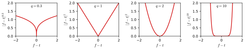
fig_4_6. Reproduces Bishop and Bishop (2024), Figure 4.6. Download: PDF · SVGResult 4.10 (Minkowski loss for \(q\ge1\) and \(q\lt 1\); Exercise 4.12, first part) p. 122, (4.40)
Fix \(\mathbf{x}\), write \(p(t)\) for \(p(t\given\mathbf{x})\), and assume \(\E|t|^q\lt \infty\).
(a) For \(q>1\), \(G_q\) is strictly convex and differentiable, and its unique minimiser \(c^\star\) is the solution of
\[ \int_{-\infty}^{c^\star}(c^\star-t)^{q-1}p(t)\d t=\int_{c^\star}^{\infty}(t-c^\star)^{q-1}p(t)\d t ; \]for \(q=2\) this is the mean.
(b) For \(q=1\), \(G_1\) is convex with one-sided derivatives \(G_1'(c^\pm)=\Pr(t\lt c)-\Pr(t>c)\pm\Pr(t=c)\); its minimisers are exactly the medians, the \(c\) with \(\Pr(t\lt c)\le\tfrac12\le\Pr(t\le c)\). For a density, \(\int_{-\infty}^{c}p=\int_c^\infty p=\tfrac12\).
(c) For \(0\lt q\lt 1\), \(G_q\) is continuous and tends to \(\infty\) as \(|c|\to\infty\), so a minimiser exists, but \(G_q\) need not be convex: it can have several local minima (bimodal densities), and the global minimiser can jump as \(q\) varies.
Proof
(a) For \(q>1\), \(u\mapsto|u|^q\) is strictly convex and continuously differentiable with derivative \(q|u|^{q-1}\sgn u\). A mixture (integral against \(p\)) of strictly convex functions of \(c\) is strictly convex. Differentiation under the integral is justified by dominated convergence (on \(|c|\le C\), \(q|c-t|^{q-1}\le q(1+|c-t|^q)\le q\{1+2^{q-1}(C^q+|t|^q)\}\), which is integrable), so \(G_q'(c)=q\int|c-t|^{q-1}\sgn(c-t)\,p(t)\d t\). Splitting the integral at \(t=c\) and setting \(G_q'=0\) gives the stated condition, which has at most one solution by strict convexity; it has one because \(G_q\to\infty\). For \(q=2\): \(\int_{-\infty}^c(c-t)p=\int_c^\infty(t-c)p\iff\int(c-t)p=0\iff c=\E[t]\).
(b) \(|c-t|\) is convex in \(c\) with right derivative \(+1\) if \(t\le c\) and \(-1\) if \(t>c\) (left derivative: \(+1\) if \(t\lt c\), \(-1\) if \(t\ge c\)). Integrating (monotone convergence for the difference quotients), \(G_1'(c^+)=\Pr(t\le c)-\Pr(t>c)\) and \(G_1'(c^-)=\Pr(t\lt c)-\Pr(t\ge c)\), the formulas stated. A convex function is minimised at \(c\) iff \(G_1'(c^-)\le0\le G_1'(c^+)\), i.e. \(\Pr(t\lt c)\le\tfrac12\le\Pr(t\le c)\). With a density, \(\Pr(t=c)=0\) and this is \(\Pr(t\lt c)=\tfrac12\).
(c) \(|c-t|^q\le|c'-t|^q+|c-c'|^q\) for \(0\lt q\le1\) (subadditivity of \(u\mapsto u^q\)), so \(|G_q(c)-G_q(c')|\le|c-c'|^q\): continuity. For \(|c|\) large, \(G_q(c)\ge\Pr(|t|\le R)(|c|-R)^q\to\infty\). Non-convexity: \(|u|^q\) is concave on each side of 0, and the bimodal density of the demo (0.3 N(−1, 0.2²) + 0.7 N(1.5, 0.7²)) gives \(G_{0.05}\) two local minima, near each peak (demo preset 5, middle panel). ∎
What happens as \(q\to0\). The usual argument (it is also the one in the official solutions to Exercise 4.12) is that \(|u|^q\) is close to 1 except in a small "notch" near \(u=0\), so the expected loss is \(1\) minus a small amount proportional to the density at \(c\), and the best \(c\) is where the density is largest. The flaw is in the word "except": since \(|u|^q=e^{q\ln|u|}=1+q\ln|u|+O(q^2)\), the loss differs from 1 by about \(q\ln|u|\) everywhere, while the notch, where \(|u|^q\le\tfrac12\), has width \(2^{-1/q}\), which is exponentially small in \(1/q\). The global first-order term wins:
Result 4.11 (the limit \(q\to0\) is not the mode in general; Exercise 4.12, last part) p. 122
Let \(p\) be a bounded density with \(\E|t|^{q_0}\lt \infty\) for some \(q_0>0\), and put
\[ \Lambda(c)=\int\ln|c-t|\,p(t)\d t . \](a) \(\Lambda\) is finite and continuous, \(\Lambda(c)\to\infty\) as \(|c|\to\infty\), and \(\{G_q(c)-1\}/q\) decreases to \(\Lambda(c)\) as \(q\downarrow0\), for every \(c\).
(b) Every limit point of minimisers \(c_q\) of \(G_q\) as \(q\to0\) minimises \(\Lambda\). In particular, if \(\Lambda\) has a unique minimiser \(c^\star\), then \(c_q\to c^\star\).
(c) If \(p\) is symmetric about \(m\) and unimodal (nonincreasing in \(|t-m|\)), then \(c^\star=m\), the mode: the book's statement holds, for instance for the Gaussian (4.8). In general \(c^\star\) is not the mode. For the Gamma density \(te^{-t}\) (mode 1, median 1.678, mean 2), \(c^\star=1.347\); for \(0.3\,\N(-1,0.2^2)+0.7\,\N(1.5,0.7^2)\) (mode \(-1\)) \(c^\star=1.412\), on the other peak.
(d) The mode is the limit of a different loss: if \(p\) is continuous with a unique global maximum at \(m\) and \(\limsup_{|t|\to\infty}p(t)\lt p(m)\), the minimisers of \(\E\,\mathbf{1}\{|c-t|>\varepsilon\}\) converge to \(m\) as \(\varepsilon\to0\).
Proof
(a) Finiteness and continuity. Near the singularity, \(\int_{|c-t|\lt 1}|\ln|c-t||\,p(t)\d t\le\|p\|_\infty\int_{-1}^1|\ln|u||\d u=2\|p\|_\infty\); away from it, \(0\le\ln|c-t|\le|c-t|^{q_0}/q_0\) (because \(\ln v\le v^{a}/a\) for \(v\ge1\), \(a>0\)), which is integrable. The same two bounds, uniform for \(c\) in a bounded set, give continuity by dominated convergence (the singular part is uniformly integrable because \(p\) is bounded). Growth: for \(|c|>R+1\), \(\Lambda(c)\ge-2\|p\|_\infty+\Pr(|t|\le R)\ln(|c|-R)\to\infty\). Monotone limit: for real \(s\), \(\psi_q(s)=(e^{qs}-1)/q\) is nondecreasing in \(q>0\) (it is the slope of the chord of the convex function \(q\mapsto e^{qs}\) from 0 to \(q\)) and tends to \(s\) as \(q\to0\). With \(s=\ln|c-t|\), \(\{G_q(c)-1\}/q=\int\psi_q(\ln|c-t|)p(t)\d t\). For \(q\le q_0\) the integrands decrease as \(q\downarrow0\) and are bounded above by the integrable \(\psi_{q_0}\), so the monotone convergence theorem gives the limit \(\Lambda(c)\).
(b) Let \(c^\star\) minimise \(\Lambda\) (it exists: \(\Lambda\) is continuous and tends to \(\infty\)) and let \(c_q\) minimise \(G_q\). By monotonicity, for \(q\le q_0\),
\[ \Lambda(c_q)\le\frac{G_q(c_q)-1}q\le\frac{G_q(c^\star)-1}q\le\frac{G_{q_0}(c^\star)-1}{q_0}=:B, \]so all \(c_q\) lie in the compact set \(\{\Lambda\le B\}\). If \(c_{q_k}\to\bar c\) along \(q_k\to0\), continuity of \(\Lambda\) and the middle inequality give \(\Lambda(\bar c)=\lim\Lambda(c_{q_k})\le\lim\{G_{q_k}(c^\star)-1\}/q_k=\Lambda(c^\star)\). So \(\bar c\) minimises \(\Lambda\); with a unique minimiser, every subsequence converges to \(c^\star\).
(c) Use \(\ln|u|=\int_0^\infty\big(\mathbf{1}\{r\lt |u|\}-\mathbf{1}\{r\lt 1\}\big)\frac{\d r}r\) (check \(|u|>1\) and \(|u|\lt 1\) separately). By Fubini (justified below),
\[ \Lambda(c)-\Lambda(m)=\int_0^\infty\Big[\Pr(|t-m|\le r)-\Pr(|t-c|\le r)\Big]\frac{\d r}{r}. \]For symmetric unimodal \(p\) and \(c>m\) (the case \(c\lt m\) is symmetric), the interval \([c-r,c+r]\) has no more mass than \([m-r,m+r]\): their mass difference is \(\int_{m+r}^{c+r}p(s)\d s-\int_{m-r}^{c-r}p(s')\d s'\), and pairing \(s\) with \(s'=s-2r\), \(|s'-m|=|(s-m)-2r|\le s-m=|s-m|\) because \(s-m\ge r\), so \(p(s')\ge p(s)\). Every integrand is therefore \(\ge0\) and \(\Lambda(c)\ge\Lambda(m)\). (Fubini: the bracket is at most \(4r\|p\|_\infty\) for small \(r\) and at most \(\Pr(|t-m|>r)+\Pr(|t-c|>r)\) for large \(r\), whose integral against \(\d r/r\) over \(r>1\) is \(\E\ln_+|t-m|+\E\ln_+|t-c|\lt \infty\).) The same formula explains the general case: minimising \(\Lambda\) maximises the probability of a window around \(c\) averaged over all radii with the scale-free weight \(\d r/r\), so a broad peak holding most of the mass beats a tall narrow one. The numbers in (c) are computed by adaptive quadrature: for the Gamma density the minimisers of \(G_q\) are 1.3808, 1.3573, 1.3505, 1.3482 at \(q=0.1,0.03,0.01,0.003\), approaching 1.3472, not 1.
(d) \(\E\,\mathbf{1}\{|c-t|>\varepsilon\}=1-\Pr(|t-c|\le\varepsilon)\), so a minimiser maximises the average of \(p\) over \([c-\varepsilon,c+\varepsilon]\). Given \(\delta>0\), the assumptions give \(\eta>0\) with \(p\le p(m)-\eta\) outside \((m-\delta,m+\delta)\). For \(\varepsilon\lt \delta\) small enough, continuity at \(m\) makes the average over \([m-\varepsilon,m+\varepsilon]\) exceed \(p(m)-\eta/2\), while any window centred at \(|c-m|\ge2\delta\) lies outside \((m-\delta,m+\delta)\) and has average at most \(p(m)-\eta\). So minimisers satisfy \(|c_\varepsilon-m|\lt 2\delta\) for small \(\varepsilon\). ∎
Note on the book and the solutions manual
The statement "the conditional mode for \(q\to0\)" (p. 122 and Exercise 4.12) is a long-standing piece of folklore; it is correct for symmetric unimodal densities, such as the Gaussian model of this chapter, where mean, median and mode coincide anyway, but false in general (Result 4.11(c)). The mode is recovered by the shrinking-window 0–1 loss of Result 4.11(d) instead. The solutions manual's "notch" argument overlooks the \(O(q)\) deviation of \(|u|^q\) from 1 outside the notch.
The Gaussian assumption makes \(p(t\given\mathbf{x})\) unimodal. Inverse problems often have multimodal conditional distributions, for which any single summary such as the mean can be poor; mixture density networks (Section 6.5 of the book) model them directly. The analogous decision theory for classification is in Chapter 5.
See also (companion course): Section 1.5.5, loss functions for regression, with Result 1.18 (the conditional mean) and Result 1.19 (Minkowski loss; it states the standard \(q\to0\) heuristic, refined by Result 4.11 here).
4.3 The Bias–Variance Trade-off
pp. 123–128 A flexible model fitted by maximum likelihood to a small data set over-fits; a penalty controls this, but how should \(\lambda\) be chosen? Not by minimising the regularised error over \(\lambda\) as well as \(\mathbf{w}\):
Filling the gap 4.6: minimising over \(\lambda\) too gives \(\lambda=0\) p. 124
Derivation
Let \(V(\lambda)=\min_{\mathbf{w}}\{E_D(\mathbf{w})+\lambda E_W(\mathbf{w})\}\). For \(0\le\lambda_1\lt \lambda_2\) with minimiser \(\mathbf{w}_2\) at \(\lambda_2\), \(V(\lambda_1)\le E_D(\mathbf{w}_2)+\lambda_1E_W(\mathbf{w}_2)\le E_D(\mathbf{w}_2)+\lambda_2E_W(\mathbf{w}_2)=V(\lambda_2)\) since \(E_W\ge0\). So \(V\) is nondecreasing and the joint minimum is at \(\lambda=0\), the unregularised (over-fitted) solution; strictly increasing when \(\mathbf{w}_2\ne\mathbf{0}\). The training error cannot choose model complexity; held-out data, or a Bayesian evidence, can. ∎
The frequentist view of model complexity imagines many data sets \(\mathcal{D}\) of size \(N\) drawn independently from \(p(\mathbf{x},t)\), each giving a fitted function \(f(\mathbf{x};\mathcal{D})\). With the regression function
\[ h(\mathbf{x})=\E[t\given\mathbf{x}]=\int t\,p(t\given\mathbf{x})\d t \tag{4.41} \]the expected squared loss of a fixed \(f\) is, by (4.39),
\[ \E[L]=\int\{f(\mathbf{x})-h(\mathbf{x})\}^2p(\mathbf{x})\d\mathbf{x}+\iint\{h(\mathbf{x})-t\}^2p(\mathbf{x},t)\d\mathbf{x}\d t. \tag{4.42} \]Consider the integrand of the first term for one data set,
\[ \{f(\mathbf{x};\mathcal{D})-h(\mathbf{x})\}^2, \tag{4.43} \]add and subtract \(\E_{\mathcal{D}}[f(\mathbf{x};\mathcal{D})]\) and expand:
\[ \begin{aligned}&\{f(\mathbf{x};\mathcal{D})-\E_{\mathcal{D}}[f(\mathbf{x};\mathcal{D})]+\E_{\mathcal{D}}[f(\mathbf{x};\mathcal{D})]-h(\mathbf{x})\}^2\\&\quad=\{f(\mathbf{x};\mathcal{D})-\E_{\mathcal{D}}[f(\mathbf{x};\mathcal{D})]\}^2+\{\E_{\mathcal{D}}[f(\mathbf{x};\mathcal{D})]-h(\mathbf{x})\}^2\\&\qquad+2\{f(\mathbf{x};\mathcal{D})-\E_{\mathcal{D}}[f(\mathbf{x};\mathcal{D})]\}\{\E_{\mathcal{D}}[f(\mathbf{x};\mathcal{D})]-h(\mathbf{x})\}.\end{aligned} \tag{4.44} \] \[ \E_{\mathcal{D}}\big[\{f(\mathbf{x};\mathcal{D})-h(\mathbf{x})\}^2\big]=\underbrace{\{\E_{\mathcal{D}}[f(\mathbf{x};\mathcal{D})]-h(\mathbf{x})\}^2}_{(\text{bias})^2}+\underbrace{\E_{\mathcal{D}}\big[\{f(\mathbf{x};\mathcal{D})-\E_{\mathcal{D}}[f(\mathbf{x};\mathcal{D})]\}^2\big]}_{\text{variance}}. \tag{4.45} \]Result 4.12 (bias–variance–noise decomposition) pp. 124–125, (4.42)–(4.49)
Let \(\mathcal{D}\) be random and independent of a test pair \((\mathbf{x},t)\sim p(\mathbf{x},t)\), with \(\E[t^2]\lt \infty\) and \(\E_{\mathcal{D}}[f(\mathbf{x};\mathcal{D})^2]\lt \infty\). Then (4.45) holds at every \(\mathbf{x}\), and the expected loss averaged over data sets and test pairs is
\[ \text{expected loss}=(\text{bias})^2+\text{variance}+\text{noise} \tag{4.46} \] \[ (\text{bias})^2=\int\{\E_{\mathcal{D}}[f(\mathbf{x};\mathcal{D})]-h(\mathbf{x})\}^2p(\mathbf{x})\d\mathbf{x} \tag{4.47} \] \[ \text{variance}=\int\E_{\mathcal{D}}\big[\{f(\mathbf{x};\mathcal{D})-\E_{\mathcal{D}}[f(\mathbf{x};\mathcal{D})]\}^2\big]p(\mathbf{x})\d\mathbf{x} \tag{4.48} \] \[ \text{noise}=\iint\{h(\mathbf{x})-t\}^2p(\mathbf{x},t)\d\mathbf{x}\d t . \tag{4.49} \]Proof
(4.45). Fix \(\mathbf{x}\) and write \(\bar f=\E_{\mathcal{D}}[f(\mathbf{x};\mathcal{D})]\), a number. Take \(\E_{\mathcal{D}}\) of (4.44): the cross term is \(2(\bar f-h(\mathbf{x}))\,\E_{\mathcal{D}}[f(\mathbf{x};\mathcal{D})-\bar f]=2(\bar f-h(\mathbf{x}))\cdot0\), because \(\bar f-h(\mathbf{x})\) does not depend on \(\mathcal{D}\) and can be taken out of the expectation.
(4.46). For a fixed data set, (4.42) is Result 4.9 applied to \(f(\cdot;\mathcal{D})\); this uses that \(t\) given \(\mathbf{x}\) has the same distribution whatever \(\mathcal{D}\) is (independence of the test pair). So \(\E_{\mathbf{x},t}[\{f(\mathbf{x};\mathcal{D})-t\}^2]=\int\{f(\mathbf{x};\mathcal{D})-h(\mathbf{x})\}^2p(\mathbf{x})\d\mathbf{x}+\text{noise}\). Average over \(\mathcal{D}\), exchange \(\E_{\mathcal{D}}\) and \(\int\d\mathbf{x}\) (Tonelli: the integrand is nonnegative), and apply (4.45) inside the integral. ∎
Flexible models have small bias and large variance, rigid ones the reverse; the best predictor balances the two. The book illustrates this with the sinusoid: \(L=100\) data sets \(\mathcal{D}^{(l)}\) of \(N=25\) points from \(h(x)=\sin(2\pi x)\) plus noise, each fitted with 24 Gaussian basis functions and a bias (25 parameters) by minimising (4.26). The empirical versions of the averages are
\[ \overline{f}(x)=\frac1L\sum_{l=1}^Lf^{(l)}(x), \tag{4.50} \] \[ (\text{bias})^2=\frac1N\sum_{n=1}^N\{\overline{f}(x_n)-h(x_n)\}^2, \tag{4.51} \] \[ \text{variance}=\frac1N\sum_{n=1}^N\frac1L\sum_{l=1}^L\{f^{(l)}(x_n)-\overline{f}(x_n)\}^2. \tag{4.52} \]Filling the gap 4.7: the estimates (4.50)–(4.52) p. 126
Derivation
The identity is exact for the empirical averages. At each \(x\), \(\frac1L\sum_l\{f^{(l)}-h\}^2=\{\overline f-h\}^2+\frac1L\sum_l\{f^{(l)}-\overline f\}^2\), by the algebra of (4.44) with \(\E_{\mathcal{D}}\) replaced by \(\frac1L\sum_l\): the cross term is \(\frac2L(\overline f-h)\sum_l(f^{(l)}-\overline f)=0\). Our 100 fits satisfy it to \(10^{-12}\).
What they estimate. The \(f^{(l)}(x)\) are independent with mean \(\E_{\mathcal{D}}f\) and variance \(v(x)\). Then \(\E[\frac1L\sum_l\{f^{(l)}-\overline f\}^2]=\frac{L-1}Lv\) (the usual divisor-\(L\) bias) and \(\E[\{\overline f-h\}^2]=\{\E_{\mathcal{D}}f-h\}^2+v/L\): the empirical squared bias is inflated by the variance of the average. With \(L=100\) both corrections are 1% of the variance.
The \(x\)-integral. (4.51)–(4.52) replace \(\int\cdot\,p(x)\d x\) by an average over points drawn from \(p(x)\). In our code \(p(x)\) is uniform on \((0,1)\) and we average over 200 equally spaced points, a quadrature rule for the same integral. The test error of Figure 4.8 is the mean squared error of each \(f^{(l)}\) on 1000 fresh points, averaged over \(l\), and estimates the left side of (4.46): at \(\ln\lambda=0\) it is 0.1197, against \(\text{bias}^2+\text{variance}+\text{noise}=0.0033+0.0233+0.0924\) (the noise term being the mean of \(\{h(x)-t\}^2\) on the same test points). ∎
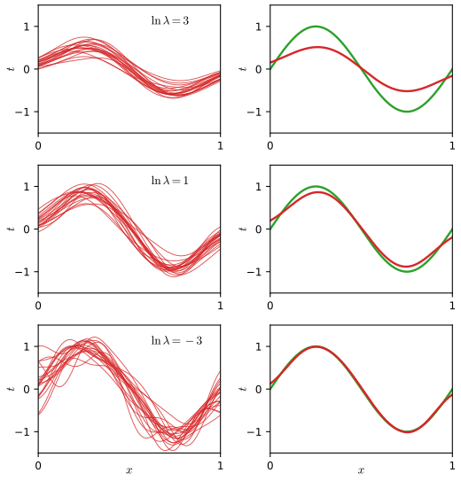
fig_4_7. Reproduces Bishop and Bishop (2024), Figure 4.7. Download: PDF · SVG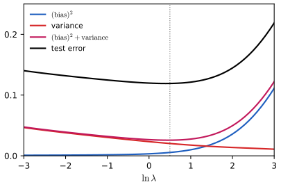
fig_4_8. Reproduces Bishop and Bishop (2024), Figure 4.8. Download: PDF · SVGFor ridge regression with the inputs held fixed, both terms can be written down, which shows the trade-off directly rather than by simulation:
Result 4.13 (bias and variance of ridge regression, fixed design) Section 4.3, complements Figures 4.7 and 4.8
Fix the training inputs, so that \(\bPhi\) is fixed and only the noise varies: \(\mathbf{t}=\mathbf{h}+\bm\epsilon\) with \(\mathbf{h}=(h(\mathbf{x}_n))_n\), \(\bm\epsilon\sim\N(\mathbf{0},\sigma^2\mathbf{I})\). The ridge prediction is linear in the targets, \(f(\mathbf{x};\mathcal{D})=\mathbf{s}(\mathbf{x})^\T\mathbf{t}\) with \(\mathbf{s}(\mathbf{x})=\bPhi(\lambda\mathbf{I}+\bPhi^\T\bPhi)^{-1}\bphi(\mathbf{x})\), so
\[ \E_{\mathcal{D}}[f(\mathbf{x};\mathcal{D})]=\mathbf{s}(\mathbf{x})^\T\mathbf{h},\qquad \text{variance at }\mathbf{x}=\sigma^2\|\mathbf{s}(\mathbf{x})\|^2=\sigma^2\sum_i\frac{d_i^2}{(d_i^2+\lambda)^2}\big(\mathbf{v}_i^\T\bphi(\mathbf{x})\big)^2 . \]The variance decreases strictly in \(\lambda\) (wherever it is nonzero) and tends to 0; as \(\lambda\to\infty\) the mean prediction tends to 0, so the squared bias tends to \(h(\mathbf{x})^2\).
Proof
By (4.27), \(f(\mathbf{x};\mathcal{D})=\bphi(\mathbf{x})^\T(\lambda\mathbf{I}+\bPhi^\T\bPhi)^{-1}\bPhi^\T\mathbf{t}=\mathbf{s}(\mathbf{x})^\T\mathbf{t}\). Linearity of expectation gives the mean \(\mathbf{s}^\T\mathbf{h}\), and \(\var(\mathbf{s}^\T\bm\epsilon)=\mathbf{s}^\T(\sigma^2\mathbf{I})\mathbf{s}\). In the SVD, \(\mathbf{s}(\mathbf{x})=\sum_i\frac{d_i}{d_i^2+\lambda}(\mathbf{v}_i^\T\bphi(\mathbf{x}))\mathbf{u}_i\), and orthonormality of the \(\mathbf{u}_i\) gives the sum; each term decreases strictly in \(\lambda\) when \(d_i\mathbf{v}_i^\T\bphi(\mathbf{x})\ne0\) and tends to 0. Similarly \(\mathbf{s}(\mathbf{x})^\T\mathbf{h}\to0\). Monte Carlo over 20000 noise draws agrees with both formulas. The bias need not be monotone at every \(\mathbf{x}\), but it is small for small \(\lambda\) when \(h\) is close to the span of the basis. ∎
Limits of the decomposition. It averages over imaginary data sets, whereas we have one; and if we really had \(L\) independent training sets we would do better to pool them into one large set. It is still the cleanest way to think about model complexity. Note also that averaging the 100 high-variance fits gave an excellent estimate of \(h\): averaging many solutions is the core of the Bayesian approach, there with respect to the posterior over \(\mathbf{w}\) rather than over data sets, and over-fitting does not arise when parameters are marginalised (Bishop, 2006).
See also (companion course): Section 3.2, the bias–variance decomposition, with Result 3.8, the closed form Result 3.9, and the link with the Bayesian \(\lambda=\alpha/\beta\) in Result 3.10; and the interactive bias–variance demo, which runs this experiment with a slider for \(\ln\lambda\).
Exercises
All 12 exercises of Chapter 4 (Bishop and Bishop, 2024, pp. 128–130), restated in my own words, with complete solutions (hidden). Stars give the book's difficulty. Each solution was worked out independently and then compared with the official solutions manual (version 1.0); the comparison is noted where there is something to say.
Exercise 4.1 (★). For the polynomial \(y(x,\mathbf{w})=\sum_{j=0}^Mw_jx^j\) of Chapter 1 and the sum-of-squares error \(E(\mathbf{w})=\tfrac12\sum_n\{y(x_n,\mathbf{w})-t_n\}^2\), show that the minimising coefficients solve the linear equations
\[ \sum_{j=0}^MA_{ij}w_j=T_i, \tag{4.53} \] \[ A_{ij}=\sum_{n=1}^N(x_n)^{i+j},\qquad T_i=\sum_{n=1}^N(x_n)^it_n. \tag{4.54} \]Solution
\(\partial y(x_n,\mathbf{w})/\partial w_i=x_n^i\), so \(\partial E/\partial w_i=\sum_n\{\sum_jw_jx_n^j-t_n\}x_n^i=\sum_j\big(\sum_nx_n^{i+j}\big)w_j-\sum_nx_n^it_n\). Setting this to zero for \(i=0,\dots,M\) is (4.53)–(4.54). These are the normal equations \(\bPhi^\T\bPhi\mathbf{w}=\bPhi^\T\mathbf{t}\) of Result 4.2 for \(\Phi_{nj}=x_n^j\) (a Vandermonde matrix), since \((\bPhi^\T\bPhi)_{ij}=\sum_nx_n^ix_n^j\); \(E\) is convex, so every solution is a minimiser, and the solution is unique when at least \(M+1\) of the \(x_n\) are distinct (the Vandermonde matrix then has full column rank). Agrees with the manual.
Exercise 4.2 (★). Write down the analogous linear equations for the regularised error \(\widetilde E(\mathbf{w})=\tfrac12\sum_n\{y(x_n,\mathbf{w})-t_n\}^2+\tfrac\lambda2\|\mathbf{w}\|^2\) of Chapter 1.
Solution
The penalty adds \(\lambda w_i\) to \(\partial E/\partial w_i\), so \(\sum_j(A_{ij}+\lambda\delta_{ij})w_j=T_i\) with \(\delta_{ij}\) the Kronecker delta: (4.27) for the polynomial basis. For \(\lambda>0\) the matrix \(\mathbf{A}+\lambda\mathbf{I}\) is positive definite and the solution unique for any data. Agrees with the manual (its \(I_{ij}\) is \(\delta_{ij}\)).
Exercise 4.3 (★). Show that \(\tanh a=(e^a-e^{-a})/(e^a+e^{-a})\) (4.55) satisfies \(\tanh(a)=2\sigma(2a)-1\) (4.56), and hence that a linear combination of logistic sigmoids \(y(x,\mathbf{w})=w_0+\sum_{j=1}^Mw_j\sigma\big((x-\mu_j)/s\big)\) (4.57) equals a combination \(y(x,\mathbf{u})=u_0+\sum_{j=1}^Mu_j\tanh\big((x-\mu_j)/2s\big)\) (4.58); relate the parameters.
Solution
See Result 4.1: \(u_j=w_j/2\) for \(j\ge1\) and \(u_0=w_0+\tfrac12\sum_jw_j\). Agrees with the manual; Result 4.1 adds the inverse map, which shows the two classes of functions are the same.
Exercise 4.4 (★★★). Show that \(\bPhi(\bPhi^\T\bPhi)^{-1}\bPhi^\T\) (4.59) projects any vector onto the span of the columns of \(\bPhi\), and deduce that the least-squares solution corresponds to the orthogonal projection of \(\mathbf{t}\) onto \(\mathcal{S}\) (Figure 4.3).
Solution
See Result 4.5: \(\mathbf{P}\) is symmetric and idempotent, its range is \(\mathcal{S}\), it fixes \(\mathcal{S}\), the residual \(\mathbf{v}-\mathbf{P}\mathbf{v}\) is orthogonal to \(\mathcal{S}\), and \(\bPhi\mathbf{w}_{\rm ML}=\mathbf{P}\mathbf{t}\). The manual shows that \(\mathbf{P}\mathbf{v}\) lies in the span and that the residual is orthogonal to each column; Result 4.5 adds idempotence and the closest-point property (Pythagoras), which together make "orthogonal projection" precise.
Exercise 4.5 (★). Each data point has a weight \(r_n>0\) and the error is
\[ E_D(\mathbf{w})=\frac12\sum_{n=1}^Nr_n\{t_n-\mathbf{w}^\T\bphi(\mathbf{x}_n)\}^2 . \tag{4.60} \]Find the minimiser \(\mathbf{w}^\star\), and interpret the weighting (i) as a data-dependent noise variance and (ii) through replicated data points.
Solution
With \(\mathbf{R}=\diag(r_1,\dots,r_N)\), \(E_D=\tfrac12(\mathbf{t}-\bPhi\mathbf{w})^\T\mathbf{R}(\mathbf{t}-\bPhi\mathbf{w})=\tfrac12\|\mathbf{R}^{1/2}\mathbf{t}-\mathbf{R}^{1/2}\bPhi\mathbf{w}\|^2\): ordinary least squares with design \(\mathbf{R}^{1/2}\bPhi\) and targets \(\mathbf{R}^{1/2}\mathbf{t}\). By Result 4.2,
\[ \mathbf{w}^\star=\big(\bPhi^\T\mathbf{R}\bPhi\big)^{-1}\bPhi^\T\mathbf{R}\mathbf{t}, \]unique when \(\bPhi\) has full column rank (\(\mathbf{R}\) is positive definite). (i) If \(t_n\sim\N(\mathbf{w}^\T\bphi_n,\sigma^2/r_n)\) independently, the negative log likelihood is \(\sum_nr_n(t_n-\mathbf{w}^\T\bphi_n)^2/(2\sigma^2)\) plus terms free of \(\mathbf{w}\): (4.60) up to the factor \(1/\sigma^2\). So \(r_n\) is a relative precision; noisy points count less. (ii) If \(r_n\) is a positive integer, \(r_n\{\cdot\}^2\) is the error of \(r_n\) copies of point \(n\): weighted least squares is ordinary least squares on the replicated data (checked numerically), and non-integer \(r_n\) is the natural extension. Agrees with the manual, whose text calls the precision \(\beta\) (the notation of Bishop 2006); in this book the noise is \(\sigma^2\), so \(r_n\) scales \(1/\sigma^2\).
Exercise 4.6 (★). Setting the gradient of (4.26) to zero, show that its minimiser is (4.27).
Solution
\(\nabla=-\bPhi^\T\mathbf{t}+\bPhi^\T\bPhi\mathbf{w}+\lambda\mathbf{w}=\mathbf{0}\iff(\lambda\mathbf{I}+\bPhi^\T\bPhi)\mathbf{w}=\bPhi^\T\mathbf{t}\). The matrix is positive definite for \(\lambda>0\), so this is the unique stationary point of a strictly convex function, hence the minimum (Result 4.7). Agrees with the manual, which omits the argument that the stationary point is a minimum.
Exercise 4.7 (★★). For a multivariate target with \(p(\mathbf{t}\given\mathbf{W},\bm\Sigma)=\N(\mathbf{t}\given\mathbf{y}(\mathbf{x},\mathbf{W}),\bm\Sigma)\) (4.61), \(\mathbf{y}(\mathbf{x},\mathbf{W})=\mathbf{W}^\T\bphi(\mathbf{x})\) (4.62), show that each column of \(\mathbf{W}_{\rm ML}\) has the form (4.14), whatever \(\bm\Sigma\) is, and that \(\bm\Sigma_{\rm ML}\) is (4.63).
Solution
See Result 4.8(b). The stationarity condition \(\bPhi^\T(\mathbf{T}-\bPhi\mathbf{W})\bm\Sigma^{-1}=\mathbf{0}\) is equivalent to \(\bPhi^\T(\mathbf{T}-\bPhi\mathbf{W})=\mathbf{0}\) because \(\bm\Sigma^{-1}\) is invertible, so \(\mathbf{W}_{\rm ML}=\bPhi^\dagger\mathbf{T}\), column \(k\) being \(\bPhi^\dagger\mathbf{t}_k\); then maximising over \(\bm\Sigma\) with \(\mathbf{W}_{\rm ML}\) plugged in gives the residual covariance (4.63). Agrees with the manual, except for two slips in its text: it says the solution "gives (4.14)" where the matrix version is (4.31), and its reference to the standard covariance result appears as "Chapter ??".
Exercise 4.8 (★). For vector targets and the expected loss \(\E[L(\mathbf{t},\mathbf{f}(\mathbf{x}))]=\iint\|\mathbf{f}(\mathbf{x})-\mathbf{t}\|^2p(\mathbf{x},\mathbf{t})\d\mathbf{x}\d\mathbf{t}\) (4.64), use the calculus of variations to show that the minimiser is \(\mathbf{f}(\mathbf{x})=\E_{\mathbf{t}}[\mathbf{t}\given\mathbf{x}]\) (4.65).
Solution
Perturb \(\mathbf{f}\to\mathbf{f}+\varepsilon\bm\eta\): \(\frac{\d}{\d\varepsilon}\E[L]\big|_0=2\int\bm\eta(\mathbf{x})^\T\big[\int\{\mathbf{f}(\mathbf{x})-\mathbf{t}\}p(\mathbf{x},\mathbf{t})\d\mathbf{t}\big]\d\mathbf{x}\). This is zero for every \(\bm\eta\) iff the bracket vanishes for (almost) every \(\mathbf{x}\): \(\mathbf{f}(\mathbf{x})p(\mathbf{x})=\int\mathbf{t}\,p(\mathbf{x},\mathbf{t})\d\mathbf{t}\), i.e. \(\mathbf{f}(\mathbf{x})=\int\mathbf{t}\,p(\mathbf{t}\given\mathbf{x})\d\mathbf{t}\). The loss is convex in \(\mathbf{f}\), so the stationary point is the minimum (or use the decomposition of Exercise 4.9). Agrees with the manual.
Exercise 4.9 (★). Expanding the square in (4.64), derive the vector analogue of (4.39) and hence that the minimiser is (4.65).
Solution
With \(\mathbf{h}(\mathbf{x})=\E[\mathbf{t}\given\mathbf{x}]\), \(\|\mathbf{f}-\mathbf{t}\|^2=\|\mathbf{f}-\mathbf{h}\|^2+2(\mathbf{f}-\mathbf{h})^\T(\mathbf{h}-\mathbf{t})+\|\mathbf{h}-\mathbf{t}\|^2\). Integrating over \(\mathbf{t}\) with \(p(\mathbf{t}\given\mathbf{x})\), the cross term becomes \(2(\mathbf{f}-\mathbf{h})^\T(\mathbf{h}-\mathbf{h})=0\) and the last term \(\E[\|\mathbf{t}-\mathbf{h}\|^2\given\mathbf{x}]=\Tr\cov[\mathbf{t}\given\mathbf{x}]\). Hence \(\E[L]=\int\|\mathbf{f}-\mathbf{h}\|^2p(\mathbf{x})\d\mathbf{x}+\int\Tr\cov[\mathbf{t}\given\mathbf{x}]\,p(\mathbf{x})\d\mathbf{x}\), minimised exactly by \(\mathbf{f}=\mathbf{h}\) (Result 4.9). The manual writes the second term as \(\var[\mathbf{t}\given\mathbf{x}]\), which for a vector must be read as the trace of the conditional covariance (the sum of the component variances).
Exercise 4.10 (★★). Rederive (4.65) by first expanding (4.64) as in (4.39).
Solution
This repeats Exercise 4.9 (the manual says the same). A variant that adds something: the expansion also identifies the minimum value, \(\min_{\mathbf{f}}\E[L]=\int\Tr\cov[\mathbf{t}\given\mathbf{x}]\,p(\mathbf{x})\d\mathbf{x}\), and shows that the excess loss of any \(\mathbf{f}\) is exactly its mean squared distance \(\int\|\mathbf{f}-\mathbf{h}\|^2p(\mathbf{x})\d\mathbf{x}\) from the regression function, the quantity decomposed into bias and variance in Section 4.3.
Exercise 4.11 (★★). The generalised Gaussian is
\[ p(x\given\sigma^2,q)=\frac{q}{2(2\sigma^2)^{1/q}\Gamma(1/q)}\exp\Big(-\frac{|x|^q}{2\sigma^2}\Big). \tag{4.66} \]Show that it is normalised (4.68), that it reduces to the Gaussian for \(q=2\), and that for \(t=y(\mathbf{x},\mathbf{w})+\epsilon\) with \(\epsilon\) drawn from (4.66) the log likelihood is
\[ \ln p(\mathbf{t}\given\mathbf{X},\mathbf{w},\sigma^2)=-\frac1{2\sigma^2}\sum_{n=1}^N|y(\mathbf{x}_n,\mathbf{w})-t_n|^q-\frac Nq\ln(2\sigma^2)+\const. \tag{4.69} \]Solution
Normalisation. By symmetry \(\int_{-\infty}^\infty e^{-|x|^q/2\sigma^2}\d x=2\int_0^\infty e^{-x^q/2\sigma^2}\d x\). Substitute \(u=x^q/(2\sigma^2)\), \(x=(2\sigma^2u)^{1/q}\), \(\d x=\tfrac1q(2\sigma^2)^{1/q}u^{1/q-1}\d u\):
\[ 2\int_0^\infty e^{-u}\tfrac1q(2\sigma^2)^{1/q}u^{1/q-1}\d u=\frac{2(2\sigma^2)^{1/q}}{q}\Gamma(1/q), \]the reciprocal of the constant in (4.66). \(q=2\): \(\Gamma(1/2)=\sqrt\pi\), so the constant is \(2/(2\sqrt{2\sigma^2}\sqrt\pi)=1/\sqrt{2\pi\sigma^2}\) and the exponent is \(-x^2/2\sigma^2\): \(\N(x\given0,\sigma^2)\). Log likelihood: each \(t_n\) has density (4.66) evaluated at \(t_n-y(\mathbf{x}_n,\mathbf{w})\); summing the logarithms, \(\ln\frac{q}{2\Gamma(1/q)}\) contributes \(N\) times a constant, \(-\tfrac1q\ln(2\sigma^2)\) contributes \(-\tfrac Nq\ln(2\sigma^2)\), and the exponents give the first term of (4.69) (with \(|t_n-y|=|y-t_n|\)). Maximising over \(\mathbf{w}\) is minimising the \(L_q\) error.
Erratum in the book
The gamma function is printed as \(\Gamma(x)=\int_{-\infty}^\infty u^{x-1}e^{-u}\d u\) (4.67). The lower limit must be 0: for \(u\lt 0\), \(u^{x-1}\) is not real for non-integer \(x\) and \(e^{-u}\) grows without bound, so the integral does not exist. The correct definition is \(\Gamma(x)=\int_0^\infty u^{x-1}e^{-u}\d u\), which is the one the manual's solution uses (and the one checked numerically).
Agrees with the manual (whose reference to the gamma-function definition appears as "(??)").
Exercise 4.12 (★★). For the expected Minkowski loss (4.40), write the condition a minimiser \(y(\mathbf{x})\) must satisfy, show that for \(q=1\) it is the conditional median, and that as \(q\to0\) the minimiser is the conditional mode.
Solution
The problem separates over \(\mathbf{x}\). For \(q>1\) the condition is \(\int_{-\infty}^{y}(y-t)^{q-1}p(t\given\mathbf{x})\d t=\int_y^\infty(t-y)^{q-1}p(t\given\mathbf{x})\d t\), and for \(q=1\) it becomes \(\int_{-\infty}^yp=\int_y^\infty p\), the median (Result 4.10, which also covers non-differentiable \(q=1\) and non-convex \(q\lt 1\)). These agree with the manual. The last part, as stated, is not true in general: as \(q\to0\) the minimisers converge to the minimiser of \(\int\ln|y-t|\,p(t\given\mathbf{x})\d t\), which is the mode for symmetric unimodal densities but not otherwise (1.347 instead of 1 for the Gamma density \(te^{-t}\); the other peak for a bimodal example). Full proof and counterexamples: Result 4.11; the mode is the limit of the window loss \(\mathbf{1}\{|y-t|>\varepsilon\}\) as \(\varepsilon\to0\) instead. The manual's argument (a narrow "notch" around \(t=y\)) neglects that \(|y-t|^q-1\approx q\ln|y-t|\) is of order \(q\) everywhere, which dominates the notch's contribution (of width \(2^{-1/q}\)).
Demonstrations for this chapter
Each demonstration runs in the browser, with seeded random numbers so that a class sees the same pictures, and links back to these notes. The ▶ Demo boxes above open them already set to the case under discussion. Each page reproduces the Python code's numbers: the fitted weights agree to \(10^{-13}\), the LMS iterates are identical bit for bit, and the Minkowski minimisers agree to \(10^{-11}\).
| Demonstration | What you can see | Sections and results |
|---|---|---|
| Linear regression with basis functions | Polynomial, Gaussian and sigmoidal bases; each weighted basis function; singular values and shrinkage factors; normal equations against the SVD. Presets: 1 Gaussian basis; 2 over-fitting polynomial; 3 ridge cure; 4 near-collinear basis; 5 sigmoids. | 4.1.1, 4.1.3, 4.1.4, 4.1.6; Results 4.2, 4.3, 4.7 |
| Sequential learning: the LMS algorithm | The path of the two weights of a straight-line fit over the error contours, for constant and decreasing learning rates, cyclic or shuffled order, raw or standardised input, and batch gradient descent. Presets: 1 small \(\eta\); 2 limit cycle; 3 divergence; 4 Robbins–Monro; 5 noise-free (Kaczmarz). | 4.1.5; Result 4.6, Filling the gap 4.3 |
| Decision theory: the Minkowski loss | A Gaussian, a skewed and a bimodal density; the expected loss \(G_q\) and its minimiser as \(q\) moves from 10 to 0.02; mean, median, mode and the true \(q\to0\) limit. Presets: 1 mean; 2 median; 3 symmetric case; 4 skewed, not the mode; 5 bimodal. | 4.2; Results 4.10, 4.11 |
The bias–variance experiment of Figures 4.7 and 4.8 is available interactively in the companion course: bias–variance demo. The Python code that produces every figure of this page is code/ch04_single_layer_regression.py (see the code index).
References
- Bishop, C. M. and Bishop, H. (2024). Deep Learning: Foundations and Concepts. Springer, Cham. Chapter 4, pp. 111–130. www.bishopbook.com.
- Bishop, C. M. (2006). Pattern Recognition and Machine Learning. Springer, New York.
- Deisenroth, M. P., Faisal, A. A. and Ong, C. S. (2020). Mathematics for Machine Learning. Cambridge University Press.
- Geman, S., Bienenstock, E. and Doursat, R. (1992). Neural networks and the bias/variance dilemma. Neural Computation, 4(1), 1–58. doi:10.1162/neco.1992.4.1.1.
- Golub, G. H. and Van Loan, C. F. (1996). Matrix Computations, 3rd edition. Johns Hopkins University Press, Baltimore.
- Hoerl, A. E. and Kennard, R. W. (1970). Ridge regression: biased estimation for nonorthogonal problems. Technometrics, 12(1), 55–67.
- Kaczmarz, S. (1937). Angenäherte Auflösung von Systemen linearer Gleichungen. Bulletin International de l'Académie Polonaise des Sciences et des Lettres A, 35, 355–357.
- Mallat, S. (1999). A Wavelet Tour of Signal Processing, 2nd edition. Academic Press.
- Penrose, R. (1955). A generalized inverse for matrices. Proceedings of the Cambridge Philosophical Society, 51, 406–413.
- Rao, C. R. and Mitra, S. K. (1971). Generalized Inverse of Matrices and Its Applications. Wiley, New York.
- Robbins, H. and Monro, S. (1951). A stochastic approximation method. Annals of Mathematical Statistics, 22(3), 400–407. doi:10.1214/aoms/1177729586.
- Widrow, B. and Hoff, M. E. (1960). Adaptive switching circuits. IRE WESCON Convention Record, 4, 96–104.
The numerical statements in the text (orthogonality of residuals, conditioning, LMS limit cycles and their \(O(\eta)\) size, ridge shrinkage, the Minkowski minimisers and their \(q\to0\) limit, and the bias–variance identities) were confirmed numerically.