Tree-Based Methods
A decision tree cuts the space of the inputs into boxes, one yes-or-no question at a time, and predicts the mean (or the majority class) of the training points in each box. Trees are easy to draw and to explain, but a single tree is a noisy predictor. This chapter grows trees by recursive binary splitting, prunes them back by cost-complexity, and then combines many trees: bagging averages trees grown on bootstrap samples, random forests also restrict each split to a random subset of the inputs, boosting adds small trees fitted to the residuals, and Bayesian additive regression trees perturb a sum of small trees by Markov chain Monte Carlo. The Hitters, Heart, Carseats and Boston data run through the chapter.
Ch. 1 Introduction Ch. 2 Statistical learning Ch. 3 Linear regression Ch. 4 Classification Ch. 5 Resampling Ch. 6 Selection and regularization Ch. 7 Beyond linearity Ch. 8 Trees Ch. 9 SVMs Ch. 10 Deep learning Ch. 11 Survival analysis Ch. 12 Unsupervised learning Ch. 13 Multiple testing
How to read these notes
They follow the book. Sections carry the book's numbers (8.1.1, 8.2.3, ...), and displayed equations that appear in the book carry its equation numbers, e.g. \((8.4)\); equations without a number are steps the book skips. Page numbers refer to the R edition (2021); the Python edition (2023) has the same text, figures and exercises a few pages later.
Filling the gaps. Where the book says that a result "can be shown", states it without proof or skips steps, an orange Filling the gap box gives the complete argument at the level of a first course in statistics. Derivations start hidden: open one with its bar, or use the button below. Green Deeper lines point to the graduate course on the same authors' larger book.
The lab in two languages. Section 8.3 shows each step in R (left) and Python (right), with the output and the figures. The Python version reproduces R's random numbers and the rules of R's tree package, so that the training sets, the cross-validation folds and every single tree are identical in the two languages; only the forests, the boosting and BART, which draw their own random numbers inside compiled code, differ by sampling noise.
Main reference
G. James, D. Witten, T. Hastie and R. Tibshirani, An Introduction to Statistical Learning with Applications in R, 2nd edition, Springer (2021), Chapter 8, pages 327–365, and G. James, D. Witten, T. Hastie, R. Tibshirani and J. Taylor, An Introduction to Statistical Learning with Applications in Python, Springer (2023), Chapter 8 (book website, with the data and the labs: www.statlearning.com). Section, equation, figure and exercise numbers below refer to these books.
The explanations, derivations, figures and code are my own; equations are cited by their numbers in the book.
Companion courses
- Statistical Learning: Theory and Methods (Hastie, Tibshirani and Friedman 2009), the graduate version of this chapter: trees in Section 9.2, bagging in Section 8.7, boosting in Chapter 10 and random forests in Chapter 15. Each section below links to the matching part.
- Bayesian and Probabilistic Machine Learning (Bishop 2006): committees, boosting and tree-based models; the Metropolis–Hastings algorithm and Gibbs sampling behind BART.
- Earlier chapters of this course: the bootstrap (Section 5.2) behind bagging, the lasso (Section 6.2.2), whose penalty (8.4) imitates, and additive models (Section 7.7), which boosted stumps build.
The chapter at a glance
- 8.1.1 A regression tree is a step function (8.9) on a partition into boxes. The boxes are found greedily: each split minimises the RSS (8.3) of its two halves, and one pass over the sorted values finds the best cutpoint of an input (Result 8.1). The large tree is then pruned: for every penalty \(\alpha\) there is a best subtree, and these subtrees are nested (Result 8.2), so cross-validation only has to choose \(\alpha\).
- 8.1.2 Classification trees grow with the Gini index (8.6) or the entropy (8.7). Both are strictly concave in the class proportions, so every split that changes the proportions lowers them, while the error rate (8.5) can stay put (Result 8.3).
- 8.2.1–8.2.2 Averaging \(B\) trees with variance \(\sigma^2\) and pairwise correlation \(\rho\) gives variance \(\rho\sigma^2+(1-\rho)\sigma^2/B\) (Result 8.4): bagging attacks the second term, random forests the first. About \(e^{-1}\approx0.368\) of the observations are left out of each bootstrap sample (Result 8.5), which gives the out-of-bag error for free.
- 8.2.3 Boosting adds shrunken small trees fitted to the residuals; the residuals of Algorithm 8.2 are always \(y_i-\hat f(x_i)\), and boosted stumps are an additive model (Result 8.6).
- 8.2.4 BART is a Bayesian sum of trees; Algorithm 8.3 is a Markov chain whose moves are accepted with a probability that involves the marginal likelihood of the leaves, available in closed form (Result 8.7).
Notation. Data \((x_i,y_i)\), \(i=1,\dots,n\), with \(p\) inputs \(X_1,\dots,X_p\). A tree \(T\) has \(|T|\) leaves (terminal nodes) \(R_1,\dots,R_{|T|}\); \(n_m\) is the number of training points in \(R_m\) and \(\hat y_{R_m}\) their mean response. For a node \(t\), \(\RSS(t)\) is the RSS of its points about their own mean, and \(T_t\) is the branch below it. In classification, \(\hat p_{mk}\) is the proportion of class \(k\) in node \(m\).
Prerequisites. Least squares (Chapter 3), the training and test error and cross-validation (Chapters 2 and 5), the bootstrap (Section 5.2), the lasso as a penalised fit (Chapter 6) and additive models (Section 7.7). For BART, the idea of a posterior distribution and of a Markov chain helps.
p. 327 Tree-based methods stratify the predictor space: they cut it into a few simple regions and predict, for a new point, the mean (regression) or the most common class (classification) of the training points in its region. The rules that define the regions can be drawn as an upside-down tree. A single tree is interpretable but rarely the most accurate method; Section 8.2 combines many trees, which costs interpretability and buys accuracy.
8.1 The Basics of Decision Trees
8.1.1 Regression Trees
pp. 328–330 An example. For the 263 baseball players of the Hitters data whose salary is known, the response is log(Salary), in thousands of dollars (the log makes the right-skewed salaries roughly symmetric), and the inputs are Years in the major leagues and Hits in the previous season. The tree of Figure 8.1 first asks whether Years < 4.5; the players with more experience are then split by Hits < 117.5. The three leaves, or terminal nodes, are the regions of Figure 8.2:
\[ R_1=\{\text{Years}<4.5\},\quad R_2=\{\text{Years}\ge4.5,\ \text{Hits}<117.5\},\quad R_3=\{\text{Years}\ge4.5,\ \text{Hits}\ge117.5\}, \]with mean log salaries 5.107, 5.998 and 6.740, i.e. predicted salaries of \(e^{5.107}\), \(e^{5.998}\) and \(e^{6.740}\) thousand dollars, about $165,000, $403,000 and $845,000. The reading is simple: experience matters most; for experienced players last season's hits matter as well; for newcomers they hardly do. The points where the space is split are internal nodes, and the segments joining nodes are branches.
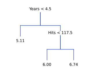
tree(), pruned to three leaves. Each label is the condition for the left branch; the number in each leaf is the mean log salary there. Code: ch08_tree_based_methods.py, fig_8_1. Reproduces James et al. (2021), Figure 8.1. Download: PDF · SVG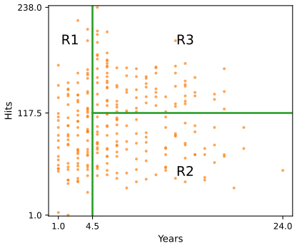
fig_8_2. Reproduces James et al. (2021), Figure 8.2. Download: PDF · SVGDefinition 8.1 (a regression tree, and the RSS it minimises) p. 330, (8.1)
A regression tree divides the predictor space into \(J\) non-overlapping boxes \(R_1,\dots,R_J\) and predicts, for every point of \(R_j\), the mean response \(\hat y_{R_j}\) of the training observations in \(R_j\). The boxes are meant to make the residual sum of squares small:
\[ \sum_{j=1}^{J}\sum_{i\in R_j}\big(y_i-\hat y_{R_j}\big)^2. \tag{8.1} \]Searching over all partitions into \(J\) boxes is computationally infeasible, so the tree is grown by recursive binary splitting: top-down (from the whole space) and greedy (each split is the best one available at that moment, without looking ahead). For an input \(X_j\) and a cutpoint \(s\), let
\[ R_1(j,s)=\{X\given X_j<s\}\quad\text{and}\quad R_2(j,s)=\{X\given X_j\ge s\}; \tag{8.2} \]the first split chooses \(j\) and \(s\) to minimise
\[ \sum_{i:\,x_i\in R_1(j,s)}\big(y_i-\hat y_{R_1}\big)^2+\sum_{i:\,x_i\in R_2(j,s)}\big(y_i-\hat y_{R_2}\big)^2. \tag{8.3} \]The same search is then applied within each resulting region, and so on, until a stopping rule holds (for example, no region with more than five observations).
Result 8.1 (the best constant is the mean, and one pass finds the best cutpoint) pp. 330–331
(a) Within a region, the constant that minimises \(\sum_{i\in R}(y_i-c)^2\) is \(c=\hat y_R\), the mean. (b) For one input, sort the \(n\) observations of the node by \(x\) and let \(S_k\) be the sum of the first \(k\) responses. A cut after the \(k\)-th observation has
\[ \text{(8.3)}=\sum_iy_i^2-\frac{S_k^2}{k}-\frac{(S_n-S_k)^2}{n-k}, \]so all \(n-1\) cutpoints are evaluated in one pass with running sums, after an \(O(n\log n)\) sort. (c) Only cuts between two distinct values of \(x\) matter, and every cut between the same two adjacent values gives the same partition; the convention is the midpoint, which is why Figure 8.1 shows 4.5 and 117.5 for integer inputs.
Filling the gap 8.1: why the mean, the one-pass formula, and why greedy is not optimal pp. 330–331
Derivation
(a) The mean. \[ \sum_{i\in R}(y_i-c)^2=\sum_{i\in R}(y_i-\hat y_R)^2+n_R(\hat y_R-c)^2 \], because the cross term \(2(\hat y_R-c)\sum_i(y_i-\hat y_R)\) vanishes. The second term is zero only for \(c=\hat y_R\). With the boxes fixed, (8.1) is therefore minimised by predicting each box's mean: a tree is least squares on the indicator columns \(\bone(X\in R_j)\), as (8.9) says.
(b) One pass. For a set of \(k\) responses with sum \(S\), \(\sum(y_i-\bar y)^2=\sum y_i^2-S^2/k\). Adding the two sides gives the display, and \(\sum_iy_i^2\) does not depend on the cut, so the best cut maximises \(S_k^2/k+(S_n-S_k)^2/(n-k)\). Moving the cut one observation to the right updates \(S_k\) by one addition. For \(p\) inputs the search costs \(O(pn\log n)\) per node; on the Hitters data the root split Years < 4.5 lowers the RSS from 207.15 to 115.06, the smallest value among the 17 admissible cuts of Years and the 122 of Hits (cuts leaving at least five players on each side). (In floating point one subtracts the node mean first, which is what the code does.)
(c) A qualitative input with \(L\) levels has \(2^{L-1}-1\) splits into two groups. For regression there is a shortcut: order the levels by their mean response; the best split puts a set of consecutive levels in this order on the left (Fisher 1958; Breiman et al. 1984), so only \(L-1\) splits need checking. R's tree() uses this ordering, which is how Carseats' ShelveLoc becomes "Bad, Medium" against "Good" in the lab.
Greedy is not optimal. A split that reduces the RSS little can enable a very good split below it. In the extreme case of an "exclusive or" pattern (\(y=1\) when exactly one of \(X_1>0\), \(X_2>0\) holds), no single split reduces the RSS at all, yet two levels of splits fit the data perfectly. This is why the book grows a large tree first and prunes afterwards, rather than stopping as soon as no split reduces the RSS by much (p. 331).
Deeper: Statistical Learning: Theory and Methods, Result 9.4 (the best constants, and one pass finds the best split point) and Result 9.8 (the ordering trick for categorical predictors).
pp. 331–333 Tree pruning. A tree grown until its leaves are tiny fits the training data well and overfits. Stopping early (split only while the RSS drops by more than a threshold) is short-sighted, for the reason just given. The better strategy is to grow a large tree \(T_0\) and prune it back to a subtree, chosen by cross-validation. There are far too many subtrees to cross-validate each one, so the search is limited to one sequence of subtrees.
Definition 8.2 (cost-complexity, or weakest-link, pruning) pp. 332–333, (8.4)
For each value of a tuning parameter \(\alpha\ge0\), let \(T_\alpha\subseteq T_0\) be the subtree that makes
\[ \sum_{m=1}^{|T|}\ \sum_{i:\,x_i\in R_m}\big(y_i-\hat y_{R_m}\big)^2+\alpha|T| \tag{8.4} \]as small as possible, \(|T|\) being the number of leaves. For \(\alpha=0\) this is the training RSS and \(T_0\) itself is best; as \(\alpha\) grows, leaves cost more and the best subtree shrinks. The penalty plays the role of the lasso's penalty (6.7): it trades fit against complexity, here counted in leaves.
Algorithm 8.1 (building a regression tree) p. 333
- Grow a large tree on the training data by recursive binary splitting, stopping only when each leaf has fewer than some minimum number of observations.
- Apply cost-complexity pruning to obtain the sequence of best subtrees \(T_\alpha\), as a function of \(\alpha\).
- Choose \(\alpha\) by \(K\)-fold cross-validation: for each fold \(k\), (a) repeat steps 1 and 2 on the other folds, and (b) compute the mean squared prediction error on fold \(k\) as a function of \(\alpha\). Average over the folds and pick the \(\alpha\) with the smallest average.
- Return the subtree of step 2 for that \(\alpha\).
Result 8.2 (the best subtrees are nested and found by collapsing weakest links) p. 333, "branches get pruned in a nested and predictable fashion"
For an internal node \(t\) of the current tree let
\[ g(t)=\frac{\RSS(t)-\RSS(T_t)}{|T_t|-1}, \]the decrease in RSS per extra leaf that the branch \(T_t\) buys. Collapsing, again and again, the internal node with the smallest \(g(t)\) gives a nested sequence \[ T_0\supset T^{(1)}\supset\dots\supset\{\text{root}\} \] and increasing values \(\alpha_1\le\alpha_2\le\dots\); the best subtree for \(\alpha\) is \(T^{(k)}\) for \(\alpha_k\le\alpha<\alpha_{k+1}\). On the Years–Hits tree of 8 leaves the sequence is 8, 7, 6, 5, 4, 3, 2, 1 leaves at \(\alpha=0\), 2.29, 3.47, 3.50, 3.79, 9.21, 23.73, 92.10: the three-leaf tree of Figure 8.1 is best for \(9.21\le\alpha<23.73\).
Filling the gap 8.2: why the subtrees are nested, and how cross-validation uses \(\alpha\) pp. 333–334 and footnote 2
Derivation
A branch is kept exactly when it pays for its leaves. Write \(C_\alpha(T)=\RSS(T)+\alpha|T|\). Replacing the branch \(T_t\) by the single leaf \(t\) changes \(C_\alpha\) by \(\RSS(t)-\RSS(T_t)-\alpha(|T_t|-1)\), which is negative (pruning helps) exactly when \(\alpha>g(t)\). The criterion is a sum over leaves, so the best subtree can be found from the bottom up: at each internal node keep the branch if its own best version costs less than the leaf, otherwise collapse. This gives a unique smallest minimiser \(T_\alpha\) for every \(\alpha\).
Nested. If \(\alpha<\alpha'\), every branch collapsed at \(\alpha\) is also collapsed at \(\alpha'\) (its comparison only becomes less favourable as \(\alpha\) grows), so \(T_{\alpha'}\subseteq T_\alpha\). Each \(C_\alpha(T)\) is a straight line in \(\alpha\) with slope \(|T|\); the best subtree is the lowest line, and as \(\alpha\) grows the lowest line can only switch to one of smaller slope. The switching points are the weakest-link values: when the node with the smallest \(g(t)\) is collapsed, the next collapse happens at a value at least as large (Breiman et al. 1984, Section 10.2). So the whole family \(\{T_\alpha\}\) is found in at most \(|T_0|-1\) steps instead of a search over all subtrees.
Numbers. The first link to go in the Years–Hits tree is the split Hits < 50.5 among players with at least 7 years and fewer than 118 hits: it lowers the RSS by only 2.29 (from 17.35 to 15.06), so it survives only for \(\alpha<2.29\). The root split, which lowers the RSS by 92.10 per extra leaf (from 207.15 to 115.06), goes last.
Cross-validation over \(\alpha\) (footnote 2). Each fold grows and prunes its own tree, whose sizes differ from those of the full tree, so the folds are compared at common values of \(\alpha\), not at common sizes. R's cv.tree() takes the \(\alpha\) values of the tree grown on all the training data and, on each fold, keeps the fold's subtree for that \(\alpha\). The CV error is then plotted against the size of the full-data tree at that \(\alpha\), which is what Figure 8.5 shows.
Deeper: Statistical Learning: Theory and Methods, Result 9.5 (a unique smallest optimal subtree for each \(\alpha\)), Result 9.6 (nested, and found by weakest-link pruning) and Filling the gap 9.5 (cross-validation indexed by \(\alpha\)).
pp. 333–335 The Hitters example. The book splits the players at random into 132 training and 131 test players, grows a large tree on nine inputs (Figure 8.4), and computes the training, six-fold cross-validation and test MSE along the pruned sequence (Figure 8.5). Here the split is R's set.seed(1); sample(263, 132), so the trees differ in detail from the book's, but the picture is the same: the CV error falls steeply up to three leaves and is nearly flat afterwards, and the test error is smallest at three leaves.
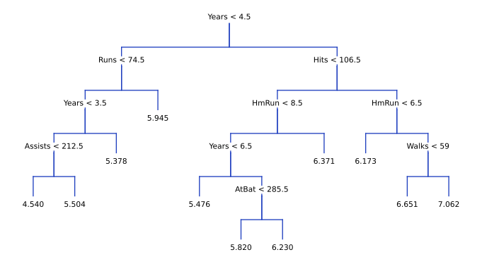
fig_8_4. Reproduces James et al. (2021), Figure 8.4. Download: PDF · SVG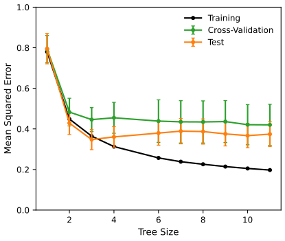
fig_8_5. Reproduces James et al. (2021), Figure 8.5. Download: PDF · SVGDeeper: Statistical Learning: Theory and Methods, Section 9.2.2 (regression trees) and Filling the gap 9.9 (the instability of trees, measured).
8.1.2 Classification Trees
pp. 335–336 A classification tree predicts the most common class among the training points of a leaf, and the class proportions in the leaf are informative too. It is grown by recursive binary splitting, but the RSS is replaced by a measure of how mixed a node is.
Definition 8.3 (classification error, Gini index, entropy) pp. 335–336, (8.5)–(8.7)
With \(\hat p_{mk}\) the proportion of training observations of class \(k\) in region \(m\):
\[ E=1-\max_k\,\hat p_{mk}, \tag{8.5} \] \[ G=\sum_{k=1}^{K}\hat p_{mk}(1-\hat p_{mk}), \tag{8.6} \] \[ D=-\sum_{k=1}^{K}\hat p_{mk}\log\hat p_{mk}. \tag{8.7} \]All three are 0 for a pure node (one class only) and largest when the classes are equally represented: \(E\le1-1/K\), \(G\le1-1/K\), \(D\le\log K\). A split is judged by the weighted average of the measure over the two children, \(\frac{n_L}{n}Q_L+\frac{n_R}{n}Q_R\). The Gini index and the entropy are used to grow trees; any of the three can be used to prune, and the error rate is the natural choice when the goal is accuracy.
Result 8.3 (Gini and entropy reward purer children; the error rate may not) p. 336, "more sensitive to node purity"
For any split of a node, the weighted average of the children's Gini indices is at most the parent's, with equality only if both children have exactly the parent's class proportions; the same holds for the entropy. For the error rate the weighted average is also at most the parent's, but it is equal to it whenever both children have the parent's majority class.
Filling the gap 8.3: concavity, the RestECG split of Figure 8.6, and what the three measures mean pp. 336–338 and Exercise 3
Derivation
Concavity. The parent's proportions are the weighted average of the children's: \(\hat p=\frac{n_L}{n}\hat p_L+\frac{n_R}{n}\hat p_R\) (counts add up). For a concave function \(Q\) of the proportions, Jensen's inequality gives \[ \frac{n_L}{n}Q(\hat p_L)+\frac{n_R}{n}Q(\hat p_R)\le Q(\hat p) \]. \(G(p)=1-\sum_kp_k^2\) is strictly concave (its Hessian is \(-2\bI\)), and so is \(D(p)=-\sum_kp_k\log p_k\) (second derivative \(-1/p_k\) in each coordinate); strictness gives equality only when \(\hat p_L=\hat p_R\). The error rate \(1-\max_kp_k\) is concave but piecewise linear: on the set where class \(k\) is the majority it equals \(1-p_k\), a linear function, and Jensen holds with equality. With two classes, Exercise 3 plots the three as functions of \(\hat p_{m1}\): \(2p(1-p)\), \(-p\log p-(1-p)\log(1-p)\) and \(\min(p,1-p)\).
The RestECG split. In the book's unpruned Heart tree a node of 20 patients, 16 with heart disease, is split into 11 patients (7 Yes) and 9 (9 Yes). Both children predict Yes, so the error rate stays at \(4/20=0.20\). The Gini index falls from \(2\cdot0.8\cdot0.2=0.320\) to \[ \frac{11}{20}\cdot2\cdot\frac{7}{11}\cdot\frac{4}{11}+\frac{9}{20}\cdot0=0.255 \], and the entropy from 0.500 to \(\frac{11}{20}\cdot0.656=0.361\). The split is made because the right child is now certain.
Two readings of the Gini index. (i) Code class \(k\) as the indicator \(\bone(y=k)\); its variance within the node is \(\hat p_{mk}(1-\hat p_{mk})\), so \(G\) is the total variance of the indicators, the classification analogue of the RSS. (ii) If points of the node were labelled at random with probabilities \(\hat p_{mk}\), the probability of a wrong label would be \(\sum_k\hat p_{mk}(1-\hat p_{mk})=G\). Near a pure node the two impurities behave alike: \(-p\log p\approx p\) and \(p(1-p)\approx p\) for small \(p\), which is why they are "quite similar numerically".
The deviance. R's tree() grows classification trees with the deviance \(-2\sum_m\sum_kn_{mk}\log\hat p_{mk}\) (lab, Section 8.3.1), which is \(2n_m\) times the entropy summed over leaves: the same criterion as (8.7), with natural logarithms.
Deeper: Statistical Learning: Theory and Methods, Result 9.7 (why Gini and deviance prefer purer splits) and Filling the gap 9.6 (two interpretations of the Gini index).
pp. 336–338 The Heart data. The response HD (here the column AHD) records heart disease for 303 patients with chest pain; 13 inputs include Age, Sex, Chol and qualitative inputs such as ChestPain (four levels) and Thal (three). A split on a qualitative input sends some levels left and the rest right; the label "ChestPain: nonanginal, nontypical, typical" in Figure 8.6 lists the levels that go left. The 297 patients without missing values are split here into 150 for training and 147 for testing; the tree is grown with the deviance and pruned with the number of misclassifications, and ten-fold cross-validation picks 5 leaves (the book's split gave 6). Like the book's tree, the unpruned tree has splits whose two leaves predict the same class (RestBP < 134 below ExAng, for example), made for the reason of Result 8.3.
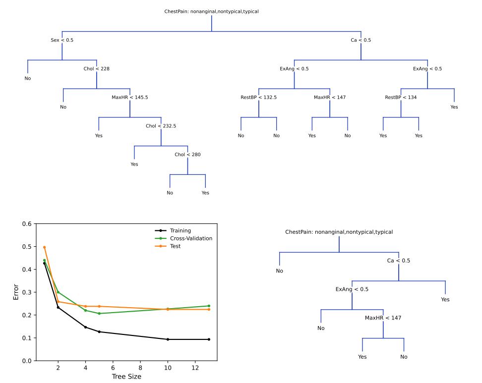
fig_8_6. Reproduces James et al. (2021), Figure 8.6. Download: PDF · SVG8.1.3 Trees Versus Linear Models
pp. 338–339 Linear regression assumes
\[ f(X)=\beta_0+\sum_{j=1}^{p}X_j\beta_j, \tag{8.8} \]and a regression tree assumes
\[ f(X)=\sum_{m=1}^{M}c_m\cdot\bone(X\in R_m), \tag{8.9} \]with \(R_1,\dots,R_M\) a partition of the predictor space. Which is better depends on the truth, and is judged by the test error (Chapter 5). Figure 8.7 shows both cases on simulated data.
Filling the gap 8.4: a tree is least squares on indicators, and a staircase is a poor diagonal p. 338, (8.9)
Derivation
(8.9) is a linear model. Given the regions, (8.9) is linear in the coefficients \(c_m\) with the \(M\) orthogonal indicator columns \(\bone(x_i\in R_m)\); least squares gives \(\hat c_m=\hat y_{R_m}\) (Filling the gap 8.1). What makes trees non-linear and adaptive is that the regions themselves are chosen from the data.
Why a tree struggles with a linear boundary. Every split is parallel to an axis, so a tree draws a boundary as a staircase. To follow the line \(x_1+x_2=0\) on \([-2,2]^2\) to within a band of half-width \(\delta\), the staircase needs steps about \(2\delta\) wide, roughly \(4/(2\delta)\) of them, each costing at least one split; a linear rule needs two coefficients. Conversely, a box-shaped region such as \(\{x_1>-0.5,\ x_2>-0.5\}\) is two splits for a tree and impossible for a single linear boundary. In Figure 8.7 (200 training points, test error on 10,000) logistic regression has test error 0.010 against the tree's 0.073 on the linear problem, and 0.133 against 0.007 on the box.
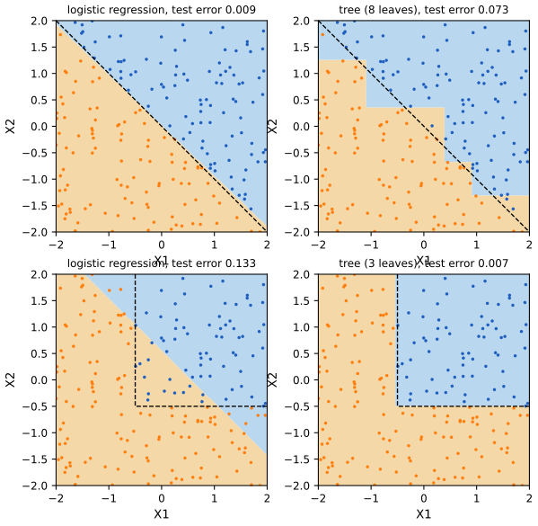
fig_8_7. Reproduces James et al. (2021), Figure 8.7 (with simulated data of my own). Download: PDF · SVGDeeper: Statistical Learning: Theory and Methods, Filling the gap 9.10 (why trees find additive structure hard).
8.1.4 Advantages and Disadvantages of Trees
pp. 339–340 For trees: they are easy to explain (easier than linear regression), they may mirror human decision making, they can be drawn and read by non-experts, and they handle qualitative inputs without dummy variables. Against: a single tree is usually less accurate than the methods of Chapters 3–7, and it is non-robust: a small change in the data can change the tree a lot, because an early split that changes rearranges everything below it (Filling the gap 9.9 of the graduate course measures this instability). Averaging many trees, Section 8.2, turns that weakness into a strength.
8.2 Bagging, Random Forests, Boosting, and Bayesian Additive Regression Trees
p. 340 An ensemble combines many simple models, often called weak learners, into one prediction. All four ensembles of this section use trees as the building block.
8.2.1 Bagging
pp. 340–341 Trees have high variance: two halves of the same data give quite different trees. Averaging reduces variance: \(n\) independent observations of variance \(\sigma^2\) have a mean of variance \(\sigma^2/n\). If we had \(B\) training sets we could average the fits, \(\hat f_{\rm avg}(x)=\frac1B\sum_{b=1}^B\hat f^b(x)\). We have one, so we use the bootstrap (Section 5.2) instead.
Definition 8.4 (bagging) p. 341
Draw \(B\) bootstrap samples (\(n\) observations drawn with replacement from the training data), fit the method to each, giving \(\hat f^{*b}\), and average:
\[ \hat f_{\rm bag}(x)=\frac1B\sum_{b=1}^{B}\hat f^{*b}(x). \]For trees, the \(B\) trees are grown deep and not pruned: each has low bias and high variance, and the averaging removes much of the variance. For classification, each tree votes and the majority class wins. \(B\) is not a critical parameter: a large \(B\) does not overfit, and it is enough to take \(B\) large enough for the error to settle (about 100 on the Heart data).
Result 8.4 (the variance of an average of correlated predictions) pp. 340–341 and p. 344
If \(Z_1,\dots,Z_B\) each have variance \(\sigma^2\) and every pair has correlation \(\rho\), then
\[ \Var\Big(\frac1B\sum_{b=1}^BZ_b\Big)=\rho\sigma^2+\frac{1-\rho}{B}\sigma^2. \]For \(\rho=0\) this is the familiar \(\sigma^2/B\). Bagged trees are identically distributed (each is a tree grown on a bootstrap sample of the same data) but positively correlated, so as \(B\to\infty\) the variance of the bagged prediction falls only to \(\rho\sigma^2\); the bias stays that of one deep tree.
Filling the gap 8.5: the variance formula, why more trees never hurt, and what averaging cannot do pp. 340–341
Derivation
The formula. \[ \Var(\sum_bZ_b)=\sum_b\Var Z_b+\sum_{b\ne b'}\Cov(Z_b,Z_{b'})=B\sigma^2+B(B-1)\rho\sigma^2 \]. Dividing by \(B^2\): \(\sigma^2/B+(1-1/B)\rho\sigma^2\), which is the display.
Which randomness? Here \(Z_b=\hat f^{*b}(x_0)\) at a fixed point, and the variance is over both the training sample and the bootstrap draws. Given the training data the trees are independent draws, so the average converges to the "ideal" bagged predictor \(\E^*\hat f^*(x_0)\) (the mean over all bootstrap samples), and its remaining variance \(\rho\sigma^2\) comes from the training data, which all trees share.
More trees never hurt (squared error). The expected squared error at \(x_0\) of the \(B\)-tree average is \[ \text{bias}^2+\rho\sigma^2+(1-\rho)\sigma^2/B+\sigma^2_\varepsilon \]: the bias does not depend on \(B\), and the variance decreases in \(B\). This is the sense in which bagging "will not lead to overfitting" as \(B\) grows; a single realisation of the test error still wobbles, as in Figure 8.8.
What averaging cannot do. Averaging leaves the bias alone: the bagged tree is about as biased as one deep tree, and nearly unbiased only because deep trees are. And because each bootstrap sample has only about 63% of the distinct observations (Result 8.5), each tree is a little worse than a tree on all the data.
Deeper: Statistical Learning: Theory and Methods, Result 15.1 (variance of an average of correlated variables), Result 8.12 (aggregation cannot increase squared error) and Result 8.13 (when aggregation helps under 0–1 loss).
pp. 341–342 Figure 8.8 shows bagging and a random forest on the Heart data. In this reproduction, after 300 trees the bagged test error is 0.190 and the random forest's 0.204, both below the single pruned tree's 0.238 (dashed); the out-of-bag errors are 0.200 and 0.193. With only 147 test patients, one patient is 0.7 percentage points, and the ordering of bagging and the forest is within that noise (in the book the forest is ahead).
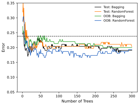
fig_8_8. Reproduces James et al. (2021), Figure 8.8. Download: PDF · SVGpp. 342–343 Out-of-bag error estimation. Each bagged tree is fitted to a bootstrap sample, which leaves out about one third of the observations. Predicting observation \(i\) with only the trees for which it was out of bag (about \(B/3\) of them), and averaging (or voting), gives an OOB prediction for every observation, and from them the OOB MSE or error rate. It is a valid estimate of the test error, because no observation is predicted by a tree that saw it.
Result 8.5 (about one third out of bag) p. 342 and footnote 3 (Exercise 5.2)
The probability that a given observation is not in a bootstrap sample of size \(n\) is \((1-1/n)^n\), which increases to \(e^{-1}=0.3679\) as \(n\to\infty\): 0.3666 for the 150 Heart training patients, 0.3672 for the 253 Boston training tracts. So each tree uses on average \(1-(1-1/n)^n\approx63.2\%\) of the distinct observations, and each observation is out of bag for about \(0.368B\) trees.
Filling the gap 8.6: the one-third, and why the OOB error is close to leave-one-out pp. 342–343
Derivation
The probability. Each of the \(n\) draws picks observation \(i\) with probability \(1/n\), independently, so \(\Pr(i\text{ never drawn})=(1-1/n)^n\). Since \[ \log(1-1/n)^n=n\log(1-1/n)=-1-\frac{1}{2n}-\frac1{3n^2}-\dots \], the limit is \(e^{-1}\), approached from below (Exercise 5.2 of Chapter 5). The number of trees for which \(i\) is out of bag is Binomial\((B,(1-1/n)^n)\): about 110 of 300 trees, with standard deviation about 8.
OOB versus leave-one-out (p. 343). For large \(B\), the OOB prediction of \(y_i\) is the average of trees grown on bootstrap samples that do not contain \(i\). Such a sample is a bootstrap sample of size \(n\) drawn from the other \(n-1\) observations. So the OOB prediction approximates the bagged predictor fitted without observation \(i\), evaluated at \(x_i\): exactly the leave-one-out prediction of the bagged model, except that its bootstrap samples are drawn from \(n-1\) points and that only about \(0.37B\) trees take part. Leave-one-out cross-validation of a bagged model would need \(n\) further forests; the OOB error comes free with one.
In the lab. R's randomForest() prints the OOB MSE as "Mean of squared residuals": 11.40 for bagging on the Boston training half (Python: 11.37). The test MSE on the other half is 23.42. The two estimate the same kind of error from different observations; that they are so far apart on this split shows how variable either estimate is with about 250 observations.
Deeper: Statistical Learning: Theory and Methods, Filling the gap 15.2 (how many trees are out of bag for a case) and Result 15.2 (the OOB estimate becomes leave-one-out cross-validation).
p. 343 Variable importance. A bagged model is no longer one tree that can be drawn. A summary of each input's importance is the total decrease in RSS (regression) or in the Gini index (classification) over all splits on that input, averaged over the \(B\) trees. Figure 8.9 shows it for the Heart data, relative to the largest.
Filling the gap 8.7: what the importances add up, and the permutation importance of the lab p. 343 and p. 359
Derivation
Impurity importance (IncNodePurity, mean decrease Gini). In one tree, a split of node \(t\) into \(t_L,t_R\) lowers the RSS by \(\Delta(t)=\RSS(t)-\RSS(t_L)-\RSS(t_R)\ge0\). Summing over all splits telescopes: \[ \sum_t\Delta(t)=\RSS(\text{root})-\RSS(\text{leaves}) \]. So the importances of the inputs add up to the total drop in training RSS achieved by the tree, shared among the inputs that made it, averaged over trees. (Each tree is measured on its own bootstrap sample, so "RSS" here is that sample's.) For classification, replace the RSS by \(n_t\) times the Gini index of the node.
Its bias. Deep trees keep splitting until the leaves are pure, and the late splits mostly fit noise. An input with many distinct values (Chol, RestBP, Age) offers many cutpoints for this, so its impurity importance is inflated relative to a binary input (Sex, Fbs). On the Heart data the continuous MaxHR ties with ChestPain for first place in Figure 8.9, whereas the book's figure has Thal, Ca and ChestPain first.
Permutation importance (%IncMSE in R). For each tree, compute the MSE on its out-of-bag observations, then again after randomly permuting the values of input \(j\) among those observations; the increase measures how much the forest relies on \(X_j\) for prediction. R averages the increases over trees and divides by their standard error. The Python lab computes both measures by hand (Forest.importance); scikit-learn's feature_importances_ is the impurity importance divided by its total.
Deeper: Statistical Learning: Theory and Methods, Filling the gap 15.3 (what the Gini importance adds up) and Result 15.3 (permutation importance in a linear model).
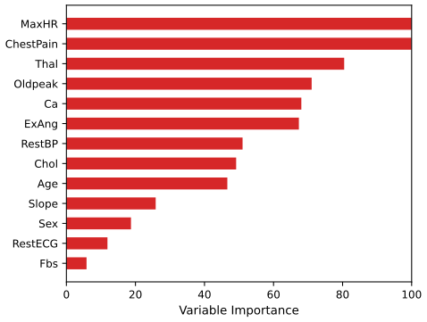
fig_8_9. Reproduces James et al. (2021), Figure 8.9. Download: PDF · SVG8.2.2 Random Forests
Definition 8.5 (random forest) pp. 343–345
As in bagging, grow \(B\) deep trees on bootstrap samples; but every time a split is considered, draw a fresh random sample of \(m\) of the \(p\) inputs, and let the split use only those. Typically \(m\approx\sqrt p\) (4 of the 13 Heart inputs); \(m=p\) is bagging. R's randomForest() uses \(m=\lfloor p/3\rfloor\) for regression and \(\lfloor\sqrt p\rfloor\) for classification by default.
p. 344 The rationale is Result 8.4. If one input is very strong, nearly every bagged tree uses it in the top split, the bagged trees look alike, and their predictions are highly correlated: \(\rho\) is large and averaging cannot remove \(\rho\sigma^2\). Forcing each split to choose from a random subset gives the other inputs a chance, decorrelates the trees, and makes their average less variable.
Filling the gap 8.8: the fraction \((p-m)/p\), and the trade-off in \(m\) p. 344
Derivation
The fraction. A random subset of \(m\) of the \(p\) inputs contains a given input with probability \(\binom{p-1}{m-1}/\binom pm=m/p\). So on average a fraction \((p-m)/p\) of the splits cannot even consider the strongest input: \(9/13=0.69\) for the Heart data with \(m=4\). The subsets are drawn afresh at every split, so the strong input still appears in most trees, but not at every node, and not always at the top.
The trade-off. In \(\rho\sigma^2+(1-\rho)\sigma^2/B\), a smaller \(m\) lowers \(\rho\); but each tree, choosing its splits among fewer candidates, fits worse, so its own variance \(\sigma^2\) and its bias tend to grow. For large \(B\) only \(\rho\sigma^2\) and the bias remain, and \(m\) is tuned (by OOB error, or cross-validation) to balance them. A small \(m\) helps most when there are many correlated inputs, as in the gene-expression example of Figure 8.10, where the 500 genes of highest variance are used. In the forest demonstration, \(m=1\) gives the least correlated trees but a worse test error.
Deeper: Statistical Learning: Theory and Methods, Section 15.4.1 (variance and the decorrelation effect), Filling the gap 15.1 (why trees from the same data are correlated) and Result 15.5 (more trees never hurt in squared error).
p. 345 Figure 8.10 (not reproduced) applies random forests with \(m=p\), \(p/2\) and \(\sqrt p\) to a gene-expression data set of 349 tissue samples and 15 classes, which is not distributed with the book; the analogue on the Boston data is Exercise 7 below (its figure). As with bagging, a forest does not overfit as \(B\) grows; \(B\) is taken large enough for the error to settle.
8.2.3 Boosting
pp. 345–346 Boosting also combines many trees, but grows them sequentially: each tree is fitted to what the previous trees have not explained, on the original data (no bootstrap). A large tree fitted to the data at once learns fast and may overfit; boosting learns slowly.
Algorithm 8.2 (boosting for regression trees) p. 347, (8.10)–(8.12)
- Set \(\hat f(x)=0\) and \(r_i=y_i\) for all \(i\) in the training set.
- For \(b=1,2,\dots,B\): (a) fit a tree \(\hat f^b\) with \(d\) splits (\(d+1\) leaves) to the training data \((X,r)\); (b) update the fit by a shrunken version of the new tree, \[ \hat f(x)\leftarrow\hat f(x)+\lambda\hat f^b(x); \tag{8.10} \] (c) update the residuals, \[ r_i\leftarrow r_i-\lambda\hat f^b(x_i). \tag{8.11} \]
- Output the boosted model \[ \hat f(x)=\sum_{b=1}^{B}\lambda\hat f^b(x). \tag{8.12} \]
Three tuning parameters: the number of trees \(B\) (boosting can overfit if \(B\) is too large, usually slowly; choose \(B\) by cross-validation); the shrinkage \(\lambda\), a small positive number such as 0.01 or 0.001 (a small \(\lambda\) needs a large \(B\)); and the number of splits \(d\), the interaction depth (\(d=1\), stumps, often works well).
Result 8.6 (what Algorithm 8.2 computes) pp. 346–347 and Exercise 2
(a) After every step, \(r_i=y_i-\hat f(x_i)\): the trees are always fitted to the current residuals, and (8.12) is the fit after \(B\) steps. (b) Each tree's leaf values are means of the current residuals, so the mean residual shrinks geometrically: \(\bar r\leftarrow(1-\lambda)\bar r\), and after \(b\) trees started from \(\hat f=0\), \(\bar r=(1-\lambda)^b\,\bar y\). (c) With stumps (\(d=1\)) each tree is a function of one input, and grouping the trees by their input gives an additive model \(\hat f(x)=\sum_{j=1}^{p}f_j(x_j)\). (d) A tree with \(d\) splits involves at most \(d\) inputs, so the boosted model has interactions of order at most \(d\).
Filling the gap 8.9: residuals, the slow start, stumps, and why boosting can overfit pp. 346–348
Derivation
(a) By induction: at the start \(r_i=y_i=y_i-0\). If \(r_i=y_i-\hat f(x_i)\) before step \(b\), then after (8.10) and (8.11) \[ r_i-\lambda\hat f^b(x_i)=y_i-(\hat f(x_i)+\lambda\hat f^b(x_i)) \]. So boosting with squared error is forward stagewise fitting: each tree is the least-squares tree for the current residuals, and only a fraction \(\lambda\) of it is kept.
(b) The slow start. A least-squares tree gives each leaf the mean residual of its points, so \(\sum_i\hat f^b(x_i)=\sum_mn_m\bar r_m=\sum_ir_i\): the tree reproduces the overall mean residual, and (8.11) multiplies it by \(1-\lambda\). Started from \(\hat f=0\), as Algorithm 8.2 is written, the fit must first learn the overall level of \(y\): on the Hitters data (mean log salary 5.93) with \(\lambda=0.001\), after 2000 trees the mean residual is still \(0.999^{2000}\times5.93=0.80\). Software starts from \(\hat f=\bar y\) instead (gbm() and scikit-learn both do), which removes this term; the boosting demonstration has both starts.
(c) Stumps make an additive model (Exercise 2). A stump on input \(j\) with cut \(s\) is \(\hat f^b(x)=c_1\bone(x_j<s)+c_2\bone(x_j\ge s)\), a function of \(x_j\) alone. Group the terms of (8.12) by input: \[ \hat f(x)=\sum_{j=1}^p\big(\sum_{b:\ j_b=j}\lambda\hat f^b(x_j)\big)=\sum_jf_j(x_j) \], each \(f_j\) a step function of one input. This is the additive model of Section 7.7, fitted one step at a time.
(d) Interaction order. The prediction of a tree on a leaf depends on the inputs used along the path to it; \(d\) splits use at most \(d\) distinct inputs, so each tree, and hence the sum, contains interactions of at most \(d\) inputs.
Why boosting can overfit but bagging cannot. Bagging averages: adding a tree moves the average towards a fixed limit. Boosting adds: each new tree reduces the training RSS a little more, and the training error keeps falling towards zero (Figure 8.13, and the boosting demonstration with \(\lambda=1\)). With small \(\lambda\) each step is tiny, so the overfitting arrives late, which is why "slow learning" works well; the number of trees then acts like a regularisation parameter, in the way the lasso's \(\lambda\) does.
Deeper: Statistical Learning: Theory and Methods, Result 10.1 (with squared error, each stage fits the current residuals), Result 10.9 (a tree with \(J\) leaves has interaction order at most \(J-1\); boosted stumps are additive), Section 10.12.1 (shrinkage) and Filling the gap 10.6 (shrinkage, stagewise fitting and the lasso).
pp. 347–348 Figure 8.11 (not reproduced; same gene-expression data as Figure 8.10) shows boosting with \(\lambda=0.01\) and depth 1 slightly ahead of depth 2, and both ahead of a random forest, with standard errors of about 0.02 that make the differences insignificant. Because each boosted tree takes the earlier trees into account, smaller trees are typically enough.
See also: boosting for classification, which the book omits, in Bayesian and Probabilistic Machine Learning, Section 14.3 (AdaBoost and the exponential error) and Statistical Learning: Theory and Methods, Section 10.10 (gradient boosting for any loss).
8.2.4 Bayesian Additive Regression Trees
pp. 348–350 BART uses \(K\) trees, like boosting builds a sum of trees in which each tree tries to capture what the others have not, and, like bagging, builds each tree in a random way. Write \(\hat f^b_k(x)\) for the prediction of the \(k\)-th tree at iteration \(b\), and \(\hat f^b(x)=\sum_{k=1}^K\hat f^b_k(x)\).
Algorithm 8.3 (Bayesian additive regression trees) p. 351
- Let \[ \hat f^1_1(x)=\hat f^1_2(x)=\dots=\hat f^1_K(x)=\frac1{nK}\sum_{i=1}^ny_i \].
- Compute \[ \hat f^1(x)=\sum_{k=1}^K\hat f^1_k(x)=\frac1n\sum_{i=1}^ny_i \].
- For \(b=2,\dots,B\): for \(k=1,2,\dots,K\): (i) for \(i=1,\dots,n\) compute the current partial residual \[ r_i=y_i-\sum_{k'<k}\hat f^b_{k'}(x_i)-\sum_{k'>k}\hat f^{b-1}_{k'}(x_i); \] (ii) fit a new tree \(\hat f^b_k\) to \(r_i\) by randomly perturbing the \(k\)-th tree of the previous iteration, \(\hat f^{b-1}_k\), favouring perturbations that improve the fit. Then compute \(\hat f^b(x)=\sum_{k=1}^K\hat f^b_k(x)\).
- Compute the mean after \(L\) burn-in iterations, \[ \hat f(x)=\frac{1}{B-L}\sum_{b=L+1}^{B}\hat f^b(x). \]
A perturbation changes the structure (adds or prunes a branch) and changes the prediction in each leaf (Figure 8.12, a schematic not reproduced here). The trees are kept small. The first \(L\) iterations (burn-in, e.g. \(L=100\) to 200) are discarded; percentiles of \(\hat f^{L+1}(x),\dots,\hat f^B(x)\) measure the uncertainty of the prediction. Typical settings: \(K=200\), \(B=1000\), \(L=100\).
p. 350 The book states, without details, that BART is a Bayesian method, that each perturbation is a draw of a tree from a posterior distribution, and that Algorithm 8.3 is a Markov chain Monte Carlo algorithm. The box below gives those details for the version that R's BART package runs (and that the Python lab writes out).
Result 8.7 (BART is Bayesian backfitting with closed-form leaf integrals) pp. 348–351
Model: \(y_i=\sum_{k=1}^Kg(x_i;T_k,M_k)+\varepsilon_i\), \(\varepsilon_i\sim\N(0,\sigma^2)\), where tree \(T_k\) has leaf values \(M_k=(\mu_{k1},\mu_{k2},\dots)\). Given all the other trees and \(\sigma\), tree \(k\) only sees the partial residuals \(r_i\) of step 3(i), as if it were the only tree. With prior \(\mu\sim\N(0,\tau^2)\) on each leaf value, a leaf containing \(n_\ell\) partial residuals with sum \(s_\ell\) has
\[ \mu\given\text{rest}\ \sim\ \N\Big(\frac{s_\ell/\sigma^2}{1/\tau^2+n_\ell/\sigma^2},\ \frac{1}{1/\tau^2+n_\ell/\sigma^2}\Big), \]and the tree structure can be compared with the leaf values integrated out: up to a factor common to all trees, each leaf contributes
\[ \sqrt{\frac{\sigma^2}{\sigma^2+n_\ell\tau^2}}\ \exp\Big(\frac{\tau^2s_\ell^2}{2\sigma^2(\sigma^2+n_\ell\tau^2)}\Big). \]A proposed birth (split a leaf into two) or death (merge two sibling leaves) is accepted with the Metropolis–Hastings probability, which multiplies the ratio of these leaf integrals by the ratio of tree priors and of proposal probabilities; then all leaf values are drawn from the normal above, and after a sweep over the \(K\) trees \(\sigma^2\) is drawn from its inverse-gamma conditional.
Filling the gap 8.10: the priors, the two closed forms, the acceptance probability, and "favouring perturbations that improve the fit" pp. 349–351
Derivation
Priors (Chipman, George and McCulloch 2010; the defaults of R's gbart()). A node at depth \(d\) is split with probability \(0.95(1+d)^{-2}\), which keeps trees small (a root splits with probability 0.95, a node at depth 2 with 0.11); the split input and cutpoint are uniform among those available. After centring \(y\), each \(\mu\sim\N(0,\tau^2)\) with \(\tau=(\max y-\min y)/(2k\sqrt K)\), \(k=2\): a sum of \(K\) leaf values then has standard deviation \(\sqrt K\tau\), half the range of \(y\) divided by \(k\), so each tree is shrunk to a small contribution. \(\sigma^2\sim\nu\lambda/\chi^2_\nu\) with \(\nu=3\) and \(\lambda\) set so that \(\Pr(\sigma<\hat\sigma_{\rm OLS})=0.9\).
Why one tree sees only the partial residuals. Given the other trees, \[ r_i=y_i-\sum_{k'\ne k}g(x_i;T_{k'},M_{k'})=g(x_i;T_k,M_k)+\varepsilon_i \]: the conditional model for tree \(k\) is a single-tree regression on \(r\). Updating the trees in turn from their conditionals is a Gibbs sampler, the Bayesian analogue of backfitting (Algorithm 7.2 in Section 7.7).
The leaf posterior. In a leaf, \(r_i\given\mu\sim\N(\mu,\sigma^2)\) independently. The log posterior of \(\mu\) is, up to a constant, \[ -\frac{\mu^2}{2\tau^2}-\sum_i\frac{(r_i-\mu)^2}{2\sigma^2}=-\frac a2\mu^2+\frac{s_\ell}{\sigma^2}\mu+\text{const} \] with \(a=1/\tau^2+n_\ell/\sigma^2\): a normal with precision \(a\) and mean \((s_\ell/\sigma^2)/a\), which shrinks the leaf mean \(s_\ell/n_\ell\) towards 0.
The leaf integral. \[ \int\prod_i\N(r_i;\mu,\sigma^2)\,\N(\mu;0,\tau^2)\,d\mu \]: the vector of residuals is jointly normal with covariance \(\sigma^2\bI+\tau^2\bone\bone^\T\). Its determinant is \(\sigma^{2n_\ell}(1+n_\ell\tau^2/\sigma^2)\) and, by the Sherman–Morrison formula, its inverse is \[ \sigma^{-2}\big(\bI-\frac{\tau^2}{\sigma^2+n_\ell\tau^2}\bone\bone^\T\big) \]. The factor \(\sum_ir_i^2\) is the same for every tree structure (every observation is in exactly one leaf), and what remains depends on the leaf only through \(n_\ell\) and \(s_\ell\): the display of Result 8.7.
The acceptance probability of a birth. Splitting leaf \(\eta\) at depth \(d\) into \(\eta_L,\eta_R\) is accepted with probability \(\min(1,A)\),
\[ A=\underbrace{\frac{p_d\,(1-p_{d+1})^2}{1-p_d}}_{\text{prior}}\cdot\underbrace{\frac{P(\text{death})/N_{\rm nog}}{P(\text{birth})/N_{\rm leaves}}}_{\text{proposal}}\cdot\underbrace{\frac{\mathcal L(\eta_L)\mathcal L(\eta_R)}{\mathcal L(\eta)}}_{\text{fit}}, \]with \(p_d=0.95(1+d)^{-2}\), \(\mathcal L\) the leaf integrals, \(N_{\rm leaves}\) the number of leaves that can be split now and \(N_{\rm nog}\) the number of nodes with two leaf children after the birth (the choice of input and cutpoint cancels between prior and proposal). A death uses the reciprocal. The "fit" factor is large when the two new leaves have clearly different mean residuals: this is the precise sense of "perturbations that improve the fit are favoured". Because a perturbation can also be rejected, or can prune, the chain explores tree structures rather than greedily refitting, which the book credits for BART's resistance to overfitting.
The noise variance. Given all trees, the residuals \(e_i=y_i-\hat f(x_i)\) are \(\N(0,\sigma^2)\) and the prior is scaled inverse-\(\chi^2\), so \[ \sigma^2\given\text{rest}=(\nu\lambda+\sum_ie_i^2)/\chi^2_{\nu+n} \].
The posterior mean. After burn-in the iterates are (dependent) draws from the posterior of \(f\), and step 4 averages them: the posterior mean, the Bayes estimate under squared error. On the Boston training half, the Python sampler written for the lab gives a test MSE of 15.39 and R's gbart() 15.92 (two runs of a Monte Carlo method with different random numbers), and both rank the inputs similarly by how often they are used in the trees, with nox near the top and crim last.
See also: the Metropolis–Hastings algorithm and Gibbs sampling in Bayesian and Probabilistic Machine Learning, Section 11.2.2 and Section 11.3, and Gibbs sampling in Statistical Learning: Theory and Methods, Section 8.6. The graduate course does not cover BART.
pp. 350–352 Figure 8.13 compares BART (probit version for the binary Heart response) with boosting as the number of iterations grows. After the burn-in the BART errors settle, with a small gap between training and test error; boosting's training error falls to zero, while its test error, after reaching its smallest value (0.163 after 244 stumps here), creeps back up to 0.19.
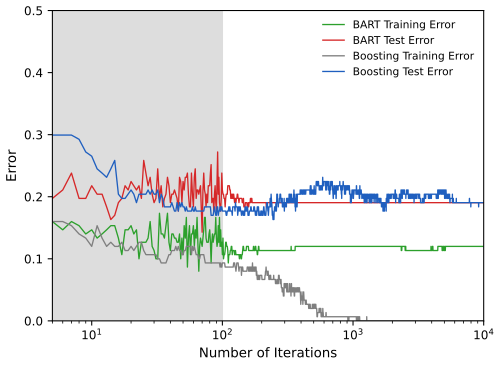
fig_8_13. Reproduces James et al. (2021), Figure 8.13. Download: PDF · SVG8.2.5 Summary of Tree Ensemble Methods
pp. 351–352 Trees are attractive weak learners: flexible, and able to mix qualitative and quantitative inputs.
| Method | Data each tree sees | How trees are grown | Combined by | Main tuning |
|---|---|---|---|---|
| Bagging | bootstrap sample | independently, deep, all inputs at every split | average or vote | \(B\) (large enough) |
| Random forest | bootstrap sample | independently, deep, \(m\) random inputs per split | average or vote | \(m\), \(B\) |
| Boosting | original data, current residuals | sequentially, small, shrunk by \(\lambda\) | sum (8.12) | \(B\), \(\lambda\), \(d\) |
| BART | original data, partial residuals | sequentially, small, random perturbations | sum, averaged over iterations | \(K\), \(B\), \(L\) (defaults work) |
The book's reading: bagged trees are similar to each other, so bagging can get stuck and explores the space of models poorly; random forests decorrelate the trees and explore more; boosting learns slowly from what is left over; BART perturbs its trees to avoid local minima.
8.3 Lab: Decision Trees
p. 353 The lab fits classification and regression trees to the Carseats and Boston data, prunes them by cross-validation, and compares bagging, random forests, boosting and BART on the Boston data. The two editions use different software: the R lab of James et al. 2021 uses the tree, randomForest, gbm and BART packages; the Python lab of James et al. 2023 uses scikit-learn and the authors' own BART code. Here the R version follows the R lab, and the Python version runs the same analyses with numpy, pandas, scipy and scikit-learn, writing out what scikit-learn does not provide (see the boxes "The helper functions"). The complete files are code/ch08_lab.R and code/ch08_lab.py; the excerpts below are taken from them verbatim.
Where the two languages differ, and why
- Same numbers: every tree.
RRandomreproduces R'sset.seed()andsample()exactly, so the training halves and the folds ofcv.tree()are the same in both languages, andRTreegrows and prunes with the rules of R'streepackage. All tree results agree exactly: the 27-leaf Carseats tree with training error 9%, the test confusion tables (accuracy 0.77, 0.775 and 0.77), the cross-validation errors 75, 75, 75, 74, 82, 83, 83, 85, 82, the 7-leaf Boston tree with test MSE 35.29, and the trees of Exercises 8 and 9. R'spredict(..., type = "class")breaks ties between classes at random; the Python code draws those ties from the same random stream. - Different random numbers: forests, boosting, BART.
randomForest(),gbm()andgbart()draw their random numbers in compiled code, so the Python versions (bootstrap samples from numpy, scikit-learn's boosting, the BART sampler of the lab) cannot match them draw for draw. The algorithms are set up the same way, and the numbers agree to within the run-to-run variation of each method: bagging 23.42 (R) and 23.06 (Python), random forest 20.07 and 19.65, boosting 18.39 and 18.32, BART 15.92 and 15.39. - Factors. R's trees split a factor by grouping its levels; scikit-learn needs numbers, so for the forests and boosting a factor becomes 0/1 columns, and "all inputs" means 11 columns for Carseats instead of R's 10 variables (Exercise 8).
- Boosting settings.
gbm()'sinteraction.depth = 4means 4 splits per tree, grown best-first, on a random half of the training data for every tree, with at least 10 observations per leaf;gbm_like()sets scikit-learn'sGradientBoostingRegressorto the same (max_leaf_nodes = 5,subsample = 0.5,min_samples_leaf = 10). The Python edition'smax_depth = 3instead allows up to 7 splits (8 leaves) and uses all the data for every tree. - The Python edition's own analysis (a 50/50 and a 70/30 split from scikit-learn, sklearn trees on 0/1 columns, pruning with
ccp_alpha) is reproduced at the end ofch08_lab.py(python_edition); its numbers are in the box The Python edition's analysis.
8.3.1 Fitting Classification Trees
Setup. In R the data come from the ISLR2 package; in Python from the book's CSV files, with string columns turned into factors (pandas categoricals, levels in alphabetical order, as R).
R
suppressPackageStartupMessages({
  library(ISLR2)
  library(tree)
  library(randomForest)
  library(gbm)
  library(BART)
  library(glmnet)
  library(class)
})
options(digits = 6, width = 100)
Python
def factors(df):
    """The book's CSV files store factors as strings: make them pandas categoricals (levels sorted, as R)."""
    df = df.copy()
    for c in df.columns:
        if df[c].dtype == object:
            df[c] = pd.Categorical(df[c])
    return df
A tree for High = (Sales > 8). Sales, in thousands of units, is turned into a binary response, and a tree is grown on the other ten variables.
R
Carseats$High <- factor(ifelse(Carseats$Sales <= 8, "No", "Yes"))   # High = Sales above 8 (thousand units)
tree.carseats <- tree(High ~ . - Sales, Carseats)
print(summary(tree.carseats))
s <- summary(tree.carseats)
keep("car_size", s$size); keep("car_dev", s$dev); keep("car_err", s$misclass[1] / 400)
Python
    Carseats = factors(common.isl_data("Carseats"))
    High = pd.Series(pd.Categorical(np.where(Carseats["Sales"] <= 8, "No", "Yes")), name="High")
    X = Carseats.drop(columns="Sales")                   # the formula High ~ . - Sales
    tree_carseats = RTree().fit(X, High)
    s = print_summary(tree_carseats)
    keep("car_size", s["size"]); keep("car_dev", s["dev"]); keep("car_err", s["error_rate"])
Variables actually used in tree construction: [1] "ShelveLoc" "Price" "Income" "CompPrice" "Population" "Advertising" [7] "Age" "US" Number of terminal nodes: 27 Residual mean deviance: 0.458 = 171 / 373 Misclassification error rate: 0.09 = 36 / 400 (both languages)
The training error is 9%. The deviance is \(-2\sum_m\sum_kn_{mk}\log\hat p_{mk}\) over the leaves, \(2n\) times the entropy (8.7) (Filling the gap 8.3), and the residual mean deviance divides it by \(n-|T_0|=400-27\). Printed, the tree lists each node with its split, size, deviance, majority class and class proportions; the root split is on shelving location.
  1) root 400 541.00 No ( 0.5900 0.4100 )
    2) ShelveLoc: Bad,Medium 315 391.00 No ( 0.6889 0.3111 )
      4) Price < 92.5 46  56.50 Yes ( 0.3043 0.6957 )
        8) Income < 57 10  12.20 No ( 0.7000 0.3000 )
         16) CompPrice < 110.5 5   0.00 No ( 1.0000 0.0000 ) *
         ...
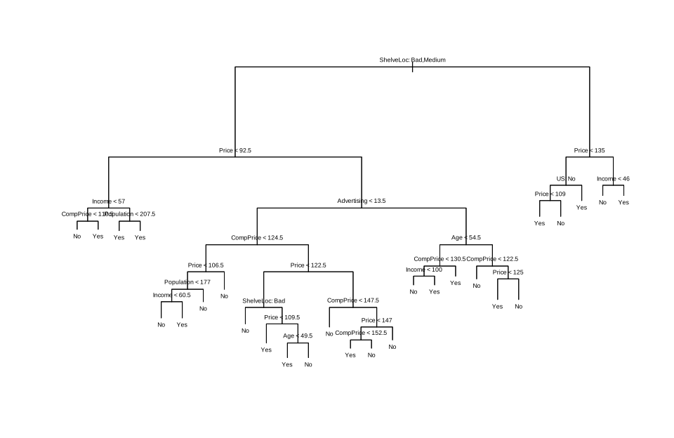
plot(tree.carseats); text(tree.carseats, pretty = 0), lab-r-carseats-tree.svg.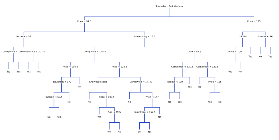
draw_tree(tree_carseats, ax), lab-py-carseats-tree.svg.The helper functions: RRandom, R's random numbers (Python)
class RRandom:
    """R's default generator: Mersenne-Twister seeded by set.seed(), with R's sample().

    unif() is R's unif_rand(); sample(n, size, replace) is R's sample(n, size, replace) for R >= 3.6
    (rejection sampling of random bits). RRandom(1).sample(506, 253) is set.seed(1); sample(506, 253).
    """
    N, M = 624, 397

    def __init__(self, seed):
        s = seed & 0xffffffff
        for _ in range(50):                      # set.seed() scrambles the seed first
            s = (69069 * s + 1) & 0xffffffff
        mt = []
        for _ in range(625):
            s = (69069 * s + 1) & 0xffffffff
            mt.append(s)
        self.mt, self.mti = mt[1:], self.N

    def _genrand(self):
        mt = self.mt
        if self.mti >= self.N:
            for kk in range(self.N):
                y = (mt[kk] & 0x80000000) | (mt[(kk + 1) % self.N] & 0x7fffffff)
                mt[kk] = mt[(kk + self.M) % self.N] ^ (y >> 1) ^ (0x9908b0df if y & 1 else 0)
            self.mti = 0
        y = mt[self.mti]
        self.mti += 1
        y ^= y >> 11
        y ^= (y << 7) & 0x9d2c5680
        y ^= (y << 15) & 0xefc60000
        y ^= y >> 18
        return y * 2.3283064365386963e-10

    def unif(self):
        v = self._genrand()
        return min(max(v, 0.5 * 2.328306437080797e-10), 1.0 - 0.5 * 2.328306437080797e-10)

    def _index(self, dn):                        # R_unif_index(): a uniform integer in 0..dn-1
        bits = int(math.ceil(math.log2(dn)))
        while True:
            v = 0
            for _ in range(0, bits + 1, 16):
                v = 65536 * v + int(self.unif() * 65536)
            v &= (1 << bits) - 1
            if v < dn:
                return v

    def sample(self, n, size=None, replace=False):
        """R's sample(n, size, replace): 1-based integers."""
        size = n if size is None else size
        if replace:
            return np.array([self._index(n) + 1 for _ in range(size)])
        x, out, m = list(range(n)), [], n
        for _ in range(size):
            j = self._index(m)
            out.append(x[j] + 1)
            m -= 1
            x[j] = x[m]
        return np.array(out)
The helper functions: RTree, growing a tree with R's rules (Python, the core)
    def _split_dev_sorted(self, ys, pos):
        """Deviance of the two children for each split position (left = first pos observations)."""
        n = len(ys)
        if self.ylevels is None:                 # RSS of both sides from running sums (8.3)
            z = ys - ys.mean()
            s1, s2 = np.cumsum(z), np.cumsum(z * z)
            nl = pos.astype(float)
            sl, ql = s1[pos - 1], s2[pos - 1]
            sr, qr = s1[-1] - sl, s2[-1] - ql
            return (ql - sl ** 2 / nl) + (qr - sr ** 2 / (n - nl))
        Y = np.eye(self.K)[ys]
        Cl = np.cumsum(Y, 0)[pos - 1]
        return self._class_dev(Cl) + self._class_dev(Y.sum(0) - Cl)

    def _best_split(self, idx):
        y, n, mc, best = self.y[idx], len(idx), self.mincut, None

        def better(c):
            return best is None or c < best[0] - 1e-9 * max(1.0, abs(best[0]))
        for j, kind in enumerate(self.kinds):
            x = self.X[idx, j]
            if kind == "numeric":
                o = np.argsort(x, kind="stable")
                xs, ys = x[o], y[o]
                pos = np.arange(mc, n - mc + 1)
                pos = pos[xs[pos - 1] < xs[pos]]          # cut only between distinct values
                if not len(pos):
                    continue
                dev = self._split_dev_sorted(ys, pos)
                k = int(np.argmin(dev))
                if better(dev[k]):
                    lab = "%g" % (0.5 * (xs[pos[k] - 1] + xs[pos[k]]))
                    best = (dev[k], j, float(lab), lab)
            else:
                lev = np.unique(x).astype(int)
                if len(lev) < 2:
                    continue
                if self.ylevels is None or self.K == 2:   # order the levels, then cut the ordered list
                    score = [y[x == l].mean() if self.ylevels is None else (y[x == l] == 1).mean() for l in lev]
                    order = lev[np.argsort(score, kind="stable")]
                    cands = [set(order[:m].tolist()) for m in range(1, len(order))]
                else:                                     # every subset of levels
                    cands = [set(lev[[b for b in range(len(lev)) if mask >> b & 1]].tolist())
                             for mask in range(1, 2 ** (len(lev) - 1))]
                for left in cands:
                    inl = np.isin(x, list(left))
                    if inl.sum() < mc or n - inl.sum() < mc:
                        continue
                    dev = self._dev(y[inl]) + self._dev(y[~inl])
                    if better(dev):
                        best = (dev, j, left, None)
        return best

    def _grow(self, node, idx):
        s = self._summary(idx)
        s["leaf"] = True
        self.nodes[node] = s
        self.where[idx] = node
        if s["n"] < self.minsize:
            return
        b = self._best_split(idx)
        if b is None or s["dev"] - b[0] < self.mindev * self.rootdev:
            return
        dev, j, rule, lab = b
        x = self.X[idx, j]
        left = x < rule if self.kinds[j] == "numeric" else np.isin(x, list(rule))
        s.update(leaf=False, var=j, rule=rule, cut=lab)
        self._grow(2 * node, idx[left])
        self._grow(2 * node + 1, idx[~left])
Filling the gap 8.11: the rules of R's tree() pp. 353–357
Details
The R lab grows its trees with tree()'s default controls, which decide how large \(T_0\) is. From the package's documentation and its output (checked against every tree of this lab): a node is split only if it has at least minsize = 10 observations; each child must have at least mincut = 5; a numeric input is cut at the midpoint of two adjacent distinct values; and the split must lower the deviance by at least mindev = 0.01 times the deviance of the root. The documentation describes the last rule as a condition on the node's own deviance, but the trees R builds follow the rule on the decrease: in the training tree of this section, a node of 13 cars with 12 of one class (deviance 7.05) is not split, although a split would leave children of 5 and 8 cars, because the best split lowers the deviance by 2.05, less than \(0.01\times270.0\). RTree applies the rules in this form and reproduces all of R's trees in the lab. To grow a larger tree, R's tree.control(nobs, mindev = 0) removes the last rule (p. 357).
Test error. Half the cars train the tree; the other half test it. R's sample() draws the training rows; RRandom(2).sample() draws the same rows.
R
set.seed(2)
train <- sample(1:nrow(Carseats), 200)
Carseats.test <- Carseats[-train, ]
High.test <- Carseats$High[-train]
tree.carseats <- tree(High ~ . - Sales, Carseats, subset = train)
tree.pred <- predict(tree.carseats, Carseats.test, type = "class")   # ties between classes: at random
print(table(tree.pred, High.test))
keep("car_test_acc", mean(tree.pred == High.test))
Python
    rng = RRandom(2)                                     # set.seed(2)
    train = rng.sample(len(Carseats), 200) - 1           # sample(1:nrow(Carseats), 200), 0-based
    test = np.setdiff1d(np.arange(len(Carseats)), train)
    tree_carseats = RTree().fit(X.iloc[train], High.iloc[train])
    tree_pred = tree_carseats.predict(X.iloc[test], type="class", rng=rng)   # ties broken as R does
    High_test = High.iloc[test].astype(str).to_numpy()
    print(pd.crosstab(pd.Series(tree_pred, name="tree.pred"), pd.Series(High_test, name="High.test")))
    keep("car_test_acc", np.mean(tree_pred == High_test))
High.test
tree.pred No Yes
No 104 33
Yes 13 50 accuracy (104 + 50) / 200 = 0.77 (both languages)
Pruning by cross-validation. cv.tree(..., FUN = prune.misclass) runs Algorithm 8.1 with ten folds, the number of misclassifications guiding both the pruning and the cross-validation; k is \(\alpha\) in (8.4).
R
set.seed(7)
cv.carseats <- cv.tree(tree.carseats, FUN = prune.misclass)
print(cv.carseats)
Python
    rng = RRandom(7)                                     # set.seed(7)
    rand = rng.sample(10, len(train), replace=True)      # the folds cv.tree() draws
    cv_carseats = cv_tree(tree_carseats, X.iloc[train], High.iloc[train], rand, method="misclass")
    print(cv_carseats)
$size 21 19 14 9 8 5 3 2 1 $dev 75 75 75 74 82 83 83 85 82 $k -Inf 0.0 1.0 1.4 2.0 3.0 4.0 9.0 18.0 (both languages)
Despite its name, dev is the number of cross-validation errors out of 200; the 9-leaf tree has the fewest, 74. The value \(k=0\) is not a mistake: with the misclassification count, a split whose two leaves predict the same class reduces the cost by nothing, \(g(t)=0\), so it is pruned at once (21 leaves at \(k=-\infty\), 19 at \(k=0\)).
The helper functions: weakest-link pruning and cv_tree (Python)
    def prune_path(self, method="deviance", newX=None, newy=None):
        """The weakest-link sequence: at each step collapse the internal node t with the smallest
        g(t) = (R(t) - R(T_t)) / (|T_t| - 1). Returns a list of (alpha, node collapsed, leaves, cost),
        the cost being measured on new data when newX is given."""
        R = self._node_cost(method)
        Rn = R if newX is None else self._node_cost(method, newX, newy)
        leaf = {k: v["leaf"] for k, v in self.nodes.items()}

        def stats_(t):
            if leaf[t]:
                return R[t], Rn[t], 1
            a, b = stats_(2 * t), stats_(2 * t + 1)
            return a[0] + b[0], a[1] + b[1], a[2] + b[2]

        def alive(t):
            while t > 1:
                t //= 2
                if leaf[t]:
                    return False
            return True
        _, rn0, s0 = stats_(1)
        seq = [(-np.inf, None, s0, rn0)]
        while not leaf[1]:
            best, bt = None, None
            for t in sorted(q for q in self.nodes if not leaf[q] and alive(q)):
                rt, _, st = stats_(t)
                g = (R[t] - rt) / (st - 1)
                if best is None or g < best:
                    best, bt = g, t
            leaf[bt] = True
            _, rn0, s0 = stats_(1)
            seq.append((best, bt, s0, rn0))
        return seq

def cv_tree(tree, X, y, rand, method="deviance"):
    """cv.tree(tree, rand, FUN): fold labels rand (R draws them with sample(10, n, replace = TRUE));
    on each fold a tree is grown with the default controls, pruned at the k of the full tree, and its
    deviance (or number of errors) on the held-out fold is added up."""
    init = tree.prune_sequence(method)
    X = pd.DataFrame(X).reset_index(drop=True)
    y = pd.Series(y).reset_index(drop=True)
    dev = np.zeros(len(init["k"]))
    for i in pd.unique(rand):
        tl = RTree().fit(X[rand != i], y[rand != i])
        dev += tl.prune_sequence(method, k=init["k"], newX=X[rand == i], newy=y[rand == i])["dev"]
    return dict(size=init["size"], dev=dev, k=init["k"])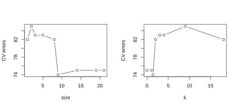
lab-r-carseats-cv.svg.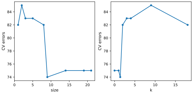
lab-py-carseats-cv.svg.R
prune.carseats <- prune.misclass(tree.carseats, best = 9)
open_svg("lab-r-carseats-pruned", 7, 4.5)
plot(prune.carseats)
text(prune.carseats, pretty = 0, cex = 0.7)
invisible(dev.off())
tree.pred <- predict(prune.carseats, Carseats.test, type = "class")
print(table(tree.pred, High.test))
keep("car_prune9_acc", mean(tree.pred == High.test))
prune.carseats <- prune.misclass(tree.carseats, best = 14)
tree.pred <- predict(prune.carseats, Carseats.test, type = "class")
print(table(tree.pred, High.test))
keep("car_prune14_acc", mean(tree.pred == High.test))
Python
    prune_carseats = tree_carseats.prune(9, method="misclass")
    fig, ax = plt.subplots(figsize=(8, 4.5))
    draw_tree(prune_carseats, ax, fontsize=8)
    common.savefig(fig, 8, "lab-py-carseats-pruned", formats=("svg",))
    tree_pred = prune_carseats.predict(X.iloc[test], type="class", rng=rng)
    print(pd.crosstab(pd.Series(tree_pred, name="tree.pred"), pd.Series(High_test, name="High.test")))
    keep("car_prune9_acc", np.mean(tree_pred == High_test))
    prune_carseats = tree_carseats.prune(14, method="misclass")
    tree_pred = prune_carseats.predict(X.iloc[test], type="class", rng=rng)
    print(pd.crosstab(pd.Series(tree_pred, name="tree.pred"), pd.Series(High_test, name="High.test")))
    keep("car_prune14_acc", np.mean(tree_pred == High_test))
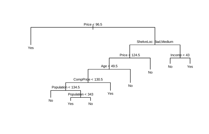
best = 9: No 97 25 / Yes 20 58 accuracy 0.775 best = 14: No 102 31 / Yes 15 52 accuracy 0.77 (both languages)
The pruned 9-leaf tree is easier to read and slightly more accurate on the test cars (77.5% against 77%); the 14-leaf tree is back at 77%. On 200 test cars these differences are one or two cars.
lab-r-carseats-pruned.svg.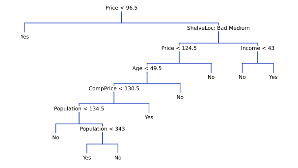
lab-py-carseats-pruned.svg.The Python edition's analysis, reproduced
The Python lab of James et al. (2023) uses scikit-learn's trees on 0/1 columns and its own random splits. python_edition() in ch08_lab.py repeats it with scikit-learn 1.5:
| Step (Python edition) | Printed in the book | Here |
|---|---|---|
| depth-3 entropy tree on all 400 cars: training accuracy | 0.7275 | 0.7900 |
| its mean log loss (called "deviance" there) | 0.4711 | 0.4711 |
| validation accuracy (200 test cars) | 0.685 | 0.685 |
| full tree on a 50/50 split: leaves; test accuracy | 35; 0.735 | 35; 0.735 |
pruned by 10-fold CV over ccp_alpha: leaves; CV accuracy; test accuracy | 30; 0.685; 0.72 | 30; 0.685; 0.72 |
| Boston, 70/30 split: pruned depth-3 tree, test MSE | 28.07 | 28.07 |
| bagging, 100 / 500 trees; random forest \(m=6\) | 14.63 / 14.61; 20.04 | 14.68 / 14.57; 20.00 |
| boosting, depth 3, 5000 trees, \(\lambda=0.001\) / 0.2 | 14.48 / 14.50 | 14.48 / 14.50 |
Everything deterministic matches. The forests differ in the second decimal because scikit-learn's random forest draws its bootstrap samples differently in recent versions. The first line is a misprint in the book (see Notes on the book).
8.3.2 Fitting Regression Trees
pp. 356–357 A regression tree for the median house value medv (in thousands of dollars) of Boston census tracts, grown on half of the 506 tracts.
R
# ================================================================== 8.3.2 regression trees
set.seed(1)
train <- sample(1:nrow(Boston), nrow(Boston) / 2)
tree.boston <- tree(medv ~ ., Boston, subset = train)
print(summary(tree.boston))
open_svg("lab-r-boston-tree", 7, 4.5)
plot(tree.boston)
text(tree.boston, pretty = 0, cex = 0.75)
invisible(dev.off())
print(tree.boston)
Python
    Boston = common.isl_data("Boston", index_col=0)
    rng = RRandom(1)                                     # set.seed(1)
    train = rng.sample(len(Boston), len(Boston) // 2) - 1
    test = np.setdiff1d(np.arange(len(Boston)), train)
    Xb, yb = Boston.drop(columns="medv"), Boston["medv"]
    tree_boston = RTree().fit(Xb.iloc[train], yb.iloc[train])
    s = print_summary(tree_boston)
    print(tree_boston.text())
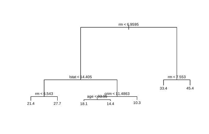
Variables actually used in tree construction: "rm" "lstat" "crim" "age"
Number of terminal nodes: 7
Residual mean deviance: 10.4 = 2550 / 246
1) root 253 19400 21.8
2) rm < 6.9595 222 6790 19.4
4) lstat < 14.405 135 1820 22.5
8) rm < 6.543 111 763 21.4 *
9) rm > 6.543 24 256 27.7 *
5) lstat > 14.405 87 1550 14.5
10) crim < 11.4863 61 614 16.2
20) age < 93.95 30 246 18.1 *
21) age > 93.95 31 164 14.4 *
11) crim > 11.4863 26 303 10.3 *
3) rm > 6.9595 31 1930 39.2
6) rm < 7.553 16 505 33.4 *
7) rm > 7.553 15 317 45.4 * (both languages)
Only four of the twelve inputs are used. For regression the deviance is the RSS. Larger houses (rm, the average number of rooms) and fewer low-status residents (lstat) go with higher values: tracts with rm \(\ge7.553\) are predicted at $45,400.
lab-r-boston-tree.svg.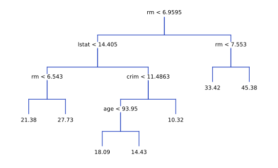
lab-py-boston-tree.svg.R
cv.boston <- cv.tree(tree.boston)                    # the folds continue the random stream of set.seed(1)
print(cv.boston)
keep("bos_cv_size", cv.boston$size); keep("bos_cv_dev", cv.boston$dev)
open_svg("lab-r-boston-cv", 4.5, 3.6)
plot(cv.boston$size, cv.boston$dev, type = "b", xlab = "size", ylab = "CV deviance (RSS)")
invisible(dev.off())
prune.boston <- prune.tree(tree.boston, best = 5)
print(prune.boston)

yhat <- predict(tree.boston, newdata = Boston[-train, ])
boston.test <- Boston[-train, "medv"]
cat("regression tree, test MSE:", mse(yhat, boston.test), "\n")
keep("bos_tree_mse", mse(yhat, boston.test))
keep("bos_prune5_mse", mse(predict(prune.boston, newdata = Boston[-train, ]), boston.test))
Python
    cv_boston = cv_tree(tree_boston, Xb.iloc[train], yb.iloc[train], rng.sample(10, len(train), replace=True))
    print(cv_boston)
    keep("bos_cv_size", cv_boston["size"]); keep("bos_cv_dev", cv_boston["dev"])
    prune_boston = tree_boston.prune(5)
    print(prune_boston.text())
    yhat = tree_boston.predict(Xb.iloc[test])
    boston_test = yb.iloc[test].to_numpy()
    print("regression tree, test MSE: %.4f" % mse(yhat, boston_test))
    keep("bos_tree_mse", mse(yhat, boston_test)); keep("bos_prune5_mse", mse(prune_boston.predict(Xb.iloc[test]), boston_test))
$size 7 6 5 4 3 2 1 $dev 4380.85 4544.82 5601.05 6171.92 6919.61 10419.47 19630.87 regression tree, test MSE: 35.2869 (pruned to 5 leaves: 35.901) (both languages)
Cross-validation picks the unpruned tree, whose test MSE is 35.29: its predictions are within about \(\sqrt{35.29}=5.94\), i.e. $5,940, of the true median value, in the root-mean-square sense. The folds of cv.tree() continue the random stream started by set.seed(1), and the Python code continues it in the same way.
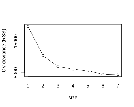
plot(cv.boston$size, cv.boston$dev, type = "b"), lab-r-boston-cv.svg.8.3.3 Bagging and Random Forests
pp. 357–359 Bagging is a random forest with \(m=p\), so both come from randomForest() in R and from Forest in Python (deep regression trees, nodes of at most 5 tracts not split, as randomForest()).
R
bag.boston <- randomForest(medv ~ ., data = Boston, subset = train, mtry = 12, importance = TRUE)
print(bag.boston)
yhat.bag <- predict(bag.boston, newdata = Boston[-train, ])
cat("bagging, 500 trees, test MSE:", mse(yhat.bag, boston.test), "\n")
keep("bag_mse", mse(yhat.bag, boston.test)); keep("bag_oob", tail(bag.boston$mse, 1))
bag.boston <- randomForest(medv ~ ., data = Boston, subset = train, mtry = 12, ntree = 25)
yhat.bag <- predict(bag.boston, newdata = Boston[-train, ])
cat("bagging, 25 trees, test MSE:", mse(yhat.bag, boston.test), "\n")
keep("bag25_mse", mse(yhat.bag, boston.test))

set.seed(1)
rf.boston <- randomForest(medv ~ ., data = Boston, subset = train, mtry = 6, importance = TRUE)
yhat.rf <- predict(rf.boston, newdata = Boston[-train, ])
cat("random forest, mtry = 6, test MSE:", mse(yhat.rf, boston.test), "\n")
keep("rf_mse", mse(yhat.rf, boston.test))
print(importance(rf.boston))
keep("rf_incmse", importance(rf.boston)[, 1]); keep("rf_purity", importance(rf.boston)[, 2])
Python
    Xn, yn = Xb.to_numpy(float), yb.to_numpy(float)
    bag_boston = Forest(m=12, ntree=500, seed=1).fit(Xn[train], yn[train])
    yhat_bag = bag_boston.predict(Xn[test])
    print("bagging, 500 trees: OOB MSE %.4f, test MSE %.4f" % (bag_boston.oob_error(), mse(yhat_bag, boston_test)))
    keep("bag_mse", mse(yhat_bag, boston_test)); keep("bag_oob", bag_boston.oob_error())
    bag25 = Forest(m=12, ntree=25, seed=2).fit(Xn[train], yn[train])
    print("bagging, 25 trees, test MSE: %.4f" % mse(bag25.predict(Xn[test]), boston_test))
    keep("bag25_mse", mse(bag25.predict(Xn[test]), boston_test))
    rf_boston = Forest(m=6, ntree=500, seed=1).fit(Xn[train], yn[train])
    yhat_rf = rf_boston.predict(Xn[test])
    print("random forest, m = 6, test MSE: %.4f" % mse(yhat_rf, boston_test))
    keep("rf_mse", mse(yhat_rf, boston_test))
    imp = rf_boston.importance().set_index(Xb.columns)
    print(imp.round(3))
keep("rf_incmse", imp["%IncMSE"]); keep("rf_purity", imp["IncNodePurity"])| Boston, test MSE on the R split | R (book) | R (here) | Python |
|---|---|---|---|
| regression tree (7 leaves) | 35.29 | 35.29 | 35.29 |
| bagging, 500 trees (OOB MSE) | 23.42 (11.40) | 23.42 (11.40) | 23.06 (11.37) |
| bagging, 25 trees | 25.75 | 25.75 | 24.62 |
| random forest, \(m=6\) | 20.07 | 20.07 | 19.65 |
The installed R packages reproduce the book's printed numbers exactly, and the importance table too (crim 19.436, 1070.42; rm 35.095, 8270.34; lstat 28.725, 5813.05; ...). Python's forests, with their own random numbers, land close. Both rank rm and lstat far ahead of the other inputs in both measures (Filling the gap 8.7).
The helper functions: Forest, bagging and random forests with OOB error and importance (Python)
class Forest:
    """Bagging (m = p) or a random forest (m < p), grown like R's randomForest().

    Each tree is grown on a bootstrap sample of the n rows (drawn with replacement), considering m
    randomly chosen inputs at every split, until the nodes are pure or have at most nodesize rows
    (5 for regression, 1 for classification), and is not pruned. The trees are scikit-learn trees.
    """

    def __init__(self, m, ntree=500, nodesize=None, classification=False, seed=0):
        self.m, self.ntree, self.classification, self.seed = m, ntree, classification, seed
        self.nodesize = nodesize if nodesize is not None else (1 if classification else 5)

    def fit(self, X, y):
        from sklearn.tree import DecisionTreeClassifier, DecisionTreeRegressor
        X, y = np.asarray(X, float), np.asarray(y)
        rng = np.random.default_rng(self.seed)
        n = len(y)
        self.trees, self.inbag = [], np.zeros((self.ntree, n), int)
        Tree = DecisionTreeClassifier if self.classification else DecisionTreeRegressor
        for b in range(self.ntree):
            idx = rng.integers(0, n, n)
            self.inbag[b] = np.bincount(idx, minlength=n)
            tr = Tree(max_features=self.m, min_samples_split=self.nodesize + 1,
                      random_state=int(rng.integers(2 ** 31 - 1)))
            self.trees.append(tr.fit(X[idx], y[idx]))
        self.X, self.y = X, y
        if self.classification:
            self.classes = self.trees[0].classes_
        return self

    def tree_predictions(self, Xn):
        """B x n matrix: each tree's prediction (class index for classification)."""
        Xn = np.asarray(Xn, float)
        if self.classification:
            return np.array([np.searchsorted(self.classes, t.predict(Xn)) for t in self.trees])
        return np.array([t.predict(Xn) for t in self.trees])

    def _combine(self, P, mask=None):
        """Average (regression) or majority vote (classification) of the rows of P, optionally only
        over the trees where mask is True."""
        mask = np.ones(P.shape, bool) if mask is None else mask
        if not self.classification:
            cnt = mask.sum(0)
            return np.where(cnt > 0, (P * mask).sum(0) / np.maximum(cnt, 1), np.nan)
        votes = np.stack([((P == k) & mask).sum(0) for k in range(len(self.classes))], 1)
        return np.where(mask.sum(0) > 0, votes.argmax(1), -1)

    def predict(self, Xn):
        out = self._combine(self.tree_predictions(Xn))
        return self.classes[out] if self.classification else out

    def oob_prediction(self):
        return self._combine(self.tree_predictions(self.X), self.inbag == 0)

    def oob_error(self):
        p = self.oob_prediction()
        if self.classification:
            ok = p >= 0
            return np.mean(self.classes[p[ok]] != self.y[ok])
        return np.nanmean((p - self.y) ** 2)

    def importance(self, permute_seed=1):
        """R's importance(): %IncMSE (mean increase in out-of-bag MSE when the input is permuted among
        each tree's out-of-bag rows, divided by its standard error) and IncNodePurity (total decrease
        in RSS from splits on the input, averaged over the trees)."""
        rng = np.random.default_rng(permute_seed)
        p = self.X.shape[1]
        purity = np.zeros(p)
        diffs = np.zeros((self.ntree, p))
        for b, t in enumerate(self.trees):
            tr = t.tree_
            for nd in range(tr.node_count):
                if tr.children_left[nd] >= 0:
                    l, r = tr.children_left[nd], tr.children_right[nd]
                    w = tr.weighted_n_node_samples
                    purity[tr.feature[nd]] += w[nd] * tr.impurity[nd] - w[l] * tr.impurity[l] - w[r] * tr.impurity[r]
            oob = np.flatnonzero(self.inbag[b] == 0)
            if not len(oob) or self.classification:
                continue
            Xo, yo = self.X[oob], self.y[oob]
            base = np.mean((t.predict(Xo) - yo) ** 2)
            for j in range(p):
                Xp = Xo.copy()
                Xp[:, j] = rng.permutation(Xp[:, j])
                diffs[b, j] = np.mean((t.predict(Xp) - yo) ** 2) - base
        mean = diffs.mean(0)
        se = np.sqrt(np.maximum((diffs ** 2).mean(0) - mean ** 2, 1e-300) / self.ntree)
        return pd.DataFrame({"%IncMSE": mean / se, "IncNodePurity": purity / self.ntree})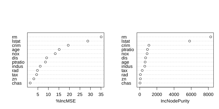
varImpPlot(rf.boston), lab-r-varimp.svg.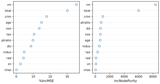
lab-py-varimp.svg.8.3.4 Boosting
pp. 359–360 Boosted regression trees with 5000 trees of interaction depth 4 (Algorithm 8.2), squared-error loss (distribution = "gaussian").
R
boost.boston <- gbm(medv ~ ., data = Boston[train, ], distribution = "gaussian",
                    n.trees = 5000, interaction.depth = 4)        # shrinkage: gbm's default, 0.1
print(summary(boost.boston, plotit = FALSE))
keep("gbm_relinf_rm", summary(boost.boston, plotit = FALSE)["rm", "rel.inf"])
keep("gbm_relinf_lstat", summary(boost.boston, plotit = FALSE)["lstat", "rel.inf"])
open_svg("lab-r-pdp", 8, 3.6)
par(mfrow = c(1, 2))
print(plot(boost.boston, i = "rm"), split = c(1, 1, 2, 1), more = TRUE)
print(plot(boost.boston, i = "lstat"), split = c(2, 1, 2, 1))
invisible(dev.off())
yhat.boost <- predict(boost.boston, newdata = Boston[-train, ], n.trees = 5000)
cat("boosting, shrinkage 0.1 (the default), test MSE:", mse(yhat.boost, boston.test), "\n")
keep("gbm_mse", mse(yhat.boost, boston.test))
boost.boston <- gbm(medv ~ ., data = Boston[train, ], distribution = "gaussian",
                    n.trees = 5000, interaction.depth = 4, shrinkage = 0.2, verbose = FALSE)
yhat.boost <- predict(boost.boston, newdata = Boston[-train, ], n.trees = 5000)
cat("boosting, shrinkage 0.2, test MSE:", mse(yhat.boost, boston.test), "\n")
keep("gbm02_mse", mse(yhat.boost, boston.test))
set.seed(1)
boost.slow <- gbm(medv ~ ., data = Boston[train, ], distribution = "gaussian",
                  n.trees = 5000, interaction.depth = 4, shrinkage = 0.001)
yhat.boost <- predict(boost.slow, newdata = Boston[-train, ], n.trees = 5000)
cat("boosting, shrinkage 0.001, test MSE:", mse(yhat.boost, boston.test), "\n")
keep("gbm0001_mse", mse(yhat.boost, boston.test))
Python
    boost_boston = gbm_like(5000, depth=4, shrinkage=0.1, seed=1).fit(Xn[train], yn[train])
    rel = pd.Series(100 * boost_boston.feature_importances_, Xb.columns).sort_values(ascending=False)
    print(rel.round(3))
    keep("gbm_relinf_rm", rel["rm"]); keep("gbm_relinf_lstat", rel["lstat"])
    fig, ax = plt.subplots(1, 2, figsize=(8, 3.6))
    for a, v in zip(ax, ("rm", "lstat")):
        j = list(Xb.columns).index(v)
        grid = np.linspace(Xn[train, j].min(), Xn[train, j].max(), 100)
        a.plot(grid, partial_dependence(boost_boston, Xn[train], j, grid))
        a.set(xlabel=v, ylabel="partial dependence of medv")
    common.savefig(fig, 8, "lab-py-pdp", formats=("svg",))
    yhat_boost = boost_boston.predict(Xn[test])
    print("boosting, shrinkage 0.1, test MSE: %.4f" % mse(yhat_boost, boston_test))
    keep("gbm_mse", mse(yhat_boost, boston_test))
    boost02 = gbm_like(5000, depth=4, shrinkage=0.2, seed=2).fit(Xn[train], yn[train])
    print("boosting, shrinkage 0.2, test MSE: %.4f" % mse(boost02.predict(Xn[test]), boston_test))
    keep("gbm02_mse", mse(boost02.predict(Xn[test]), boston_test))
    boost_slow = gbm_like(5000, depth=4, shrinkage=0.001, seed=1).fit(Xn[train], yn[train])
    print("boosting, shrinkage 0.001, test MSE: %.4f" % mse(boost_slow.predict(Xn[test]), boston_test))
keep("gbm0001_mse", mse(boost_slow.predict(Xn[test]), boston_test))| Boston, boosting | R (book) | R (here) | Python |
|---|---|---|---|
| relative influence of rm / lstat | 44.48 / 32.70 | 44.48 / 32.70 | 41.69 / 30.37 |
| test MSE, shrinkage 0.1 (the default) | 18.39 | 18.39 | 18.32 |
| test MSE, shrinkage 0.2 | 16.55 | 17.39 | 19.09 |
| test MSE, shrinkage 0.001 | (not run) | 21.50 | 21.37 |
The book attributes 18.39 to the shrinkage 0.001; it was in fact computed with gbm()'s default 0.1 (Notes on the book): with 0.001, 5000 trees are not enough and the test MSE is 21.5. The run with shrinkage 0.2 starts from the random state left by the first run in R, which changes its half-samples; between versions and languages it varies from 16.6 to 19.1, a reminder that one train/test split and one random run decide such comparisons only roughly.
The helper functions: gbm_like and partial_dependence (Python)
def gbm_like(n_trees, depth=1, shrinkage=0.1, classification=False, seed=0):
    """scikit-learn's gradient boosting with the defaults of R's gbm(): interaction.depth = d splits per
    tree (max_leaf_nodes = d + 1, grown best-first), half of the training rows drawn afresh for every
    tree (bag.fraction = 0.5), at least 10 rows per leaf, squared error or Bernoulli deviance."""
    from sklearn.ensemble import GradientBoostingClassifier, GradientBoostingRegressor
    G = GradientBoostingClassifier if classification else GradientBoostingRegressor
    return G(n_estimators=n_trees, learning_rate=shrinkage, max_leaf_nodes=depth + 1, max_depth=None,
             subsample=0.5, min_samples_leaf=10, random_state=seed)


def partial_dependence(model, X, j, grid):
    """Partial dependence of the fit on input j: the average prediction over the data with input j
    set to each grid value (the other inputs are 'integrated out' over their observed values)."""
    X = np.asarray(X, float)
    out = []
    for g in grid:
        Xc = X.copy()
        Xc[:, j] = g
        out.append(model.predict(Xc).mean())
    return np.array(out)
Filling the gap 8.12: relative influence and partial dependence p. 360
Details
Relative influence (summary(boost.boston)) is the impurity importance of Filling the gap 8.7 for a boosted model: the RSS reductions of all splits on an input, summed over the trees and scaled to add to 100. scikit-learn's feature_importances_ is the same quantity scaled to add to 1.
Partial dependence. For an input \(X_j\), the partial dependence function is \(\bar f_j(x)=\frac1n\sum_{i=1}^n\hat f(x,x_{i,-j})\): set \(X_j=x\) for every observation, keep their other inputs, and average the predictions. It shows the effect of \(X_j\) "after integrating out the other variables" (the book's words), averaged over their observed values. For an additive model \(\hat f=\sum_kf_k(x_k)\) it recovers \(f_j\) up to a constant; when \(X_j\) interacts with other inputs it is an average of differently shaped curves. Here medv rises steeply with rm above 7 rooms and falls with lstat up to about 20%.
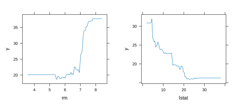
plot(boost.boston, i = "rm") and i = "lstat", lab-r-pdp.svg.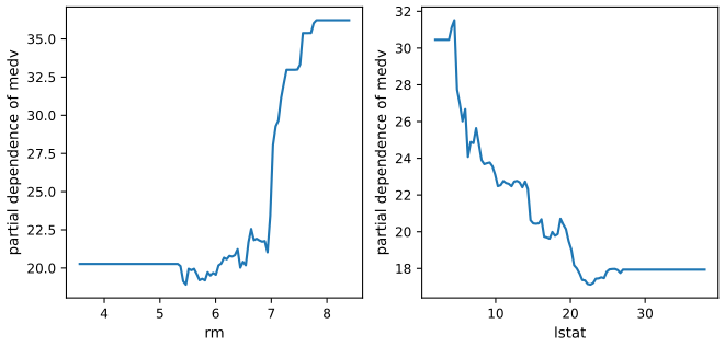
lab-py-pdp.svg.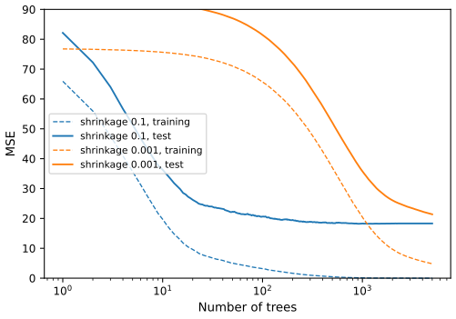
staged_predict), as in the Python edition, for shrinkage 0.1 and 0.001; lab-py-boost-curve.svg.8.3.5 Bayesian Additive Regression Trees
pp. 360–361 BART with its default settings: 200 trees, 100 burn-in iterations, 1000 kept draws.
R
x <- Boston[, 1:12]
y <- Boston[, "medv"]
xtrain <- x[train, ]; ytrain <- y[train]
xtest <- x[-train, ]; ytest <- y[-train]
set.seed(1)
quiet(bartfit <- gbart(xtrain, ytrain, x.test = xtest))
yhat.bart <- bartfit$yhat.test.mean
cat("BART, test MSE:", mse(ytest, yhat.bart), "\n")
keep("bart_mse", mse(ytest, yhat.bart)); keep("bart_sigma", mean(bartfit$sigma[-(1:100)]))
ord <- order(bartfit$varcount.mean, decreasing = TRUE)
print(bartfit$varcount.mean[ord])
keep("bart_varcount", bartfit$varcount.mean)
Python
    bartfit = BART(seed=1).fit(Xn[train], yn[train], Xn[test])   # K = 200, 100 burn-in, 1000 draws
    yhat_bart = bartfit.yhat_test.mean(0)
    print("BART, test MSE: %.4f" % mse(yhat_bart, boston_test))
    keep("bart_mse", mse(yhat_bart, boston_test)); keep("bart_sigma", bartfit.sigma.mean())
    vc = pd.Series(bartfit.varcount.mean(0), Xb.columns)
    print(vc.sort_values(ascending=False).round(2))
    keep("bart_varcount", vc)
R: BART, test MSE: 15.9191 (book: 15.95)
nox 22.97 lstat 21.65 rad 21.64 rm 20.73 tax 20.02 ptratio 19.62 chas 19.28 age 19.28
indus 19.07 zn 15.58 dis 13.80 crim 11.61
Python: BART, test MSE: 15.3929
nox 25.63 rad 23.83 tax 23.68 lstat 22.79 rm 22.43 chas 21.83 ptratio 21.68 age 20.72
indus 20.27 zn 16.03 dis 15.31 crim 12.37
BART has the lowest test MSE of the lab's methods in both languages. The last numbers are the average number of splits on each input over the 200 trees of a draw; unlike the importance measures above, they count how often an input is used, not how much it helps (rm and lstat, the most important inputs for the forests, are used about as often as chas, a 0/1 input).
The helper functions: BART, the sampler of Algorithm 8.3 (Python, the main loop and the birth–death move)
            for t in range(K):
                T = trees[t]
                r = resp - (fit - tfit[t])                       # partial residual, step 3(a)i
                self._move(T, leaf[t], r, XI, sig2, tau2, rng, leafT[t] if nt else None, XIt)
                L, nn = leaf[t], len(T.var)
                cnt, sm = np.bincount(L, minlength=nn), np.bincount(L, weights=r, minlength=nn)
                b = np.array(T.bots())
                a = 1.0 / tau2 + cnt[b] / sig2                     # leaf posterior precision
                mu = sm[b] / sig2 / a + rng.standard_normal(len(b)) / np.sqrt(a)
                muv = np.zeros(nn)
                muv[b] = mu
                for bi, mi in zip(b, mu):
                    T.mu[bi] = mi
                new = muv[L]
                fit += new - tfit[t]
                tfit[t] = new
                if nt:
                    newT = muv[leafT[t]]
                    fitT += newT - tfitT[t]
                    tfitT[t] = newT

    def _move(self, T, L, r, XI, sig2, tau2, rng, LT, XIt):
        """One birth or death proposal for tree T, accepted with the Metropolis-Hastings probability."""
        bots = T.bots()
        good = [b for b in bots if len(T.goodvars(b))]
        pb = 0.0 if not good else (1.0 if len(bots) == 1 else 0.5)
        if rng.random() < pb:                                       # birth
            i = good[rng.integers(len(good))]
            gv = T.goodvars(i)
            v = gv[rng.integers(len(gv))]
            c = T.lo[i][v] + rng.integers(T.hi[i][v] - T.lo[i][v])
            inn = L == i
            gl = inn & (XI[:, v] <= c)
            gr = inn & ~gl
            nl, nr = int(gl.sum()), int(gr.sum())
            if nl < self.minobs or nr < self.minobs:
                return
            sl, sr = r[gl].sum(), r[gr].sum()
            d1 = T.depth[i] + 1
            lo_l, hi_l, lo_r, hi_r = T.lo[i].copy(), T.hi[i].copy(), T.lo[i].copy(), T.hi[i].copy()
            hi_l[v], lo_r[v] = c, c + 1
            PGn = self._pgrow(T.depth[i], T.lo[i], T.hi[i])
            PGl, PGr = self._pgrow(d1, lo_l, hi_l), self._pgrow(d1, lo_r, hi_r)
            par = T.parent[i]
            par_nog = par != -1 and T.left[T.left[par]] == -1 and T.left[T.right[par]] == -1
            nog_new = len(T.nogs()) + 1 - int(par_nog)
            good_new = len(good) - 1 + (PGl > 0) + (PGr > 0)
            PDy = 0.5 if good_new > 0 else 1.0                      # P(death) in the proposed tree
            la = (np.log(PGn) + np.log1p(-PGl) + np.log1p(-PGr) - np.log1p(-PGn)
                  + np.log(PDy) - np.log(nog_new) - np.log(pb) + np.log(len(good))
                  + self._lml(nl, sl, sig2, tau2) + self._lml(nr, sr, sig2, tau2)
                  - self._lml(nl + nr, sl + sr, sig2, tau2))
            if np.log(rng.random()) < la:
                li, ri = T.new_node(i, d1, lo_l, hi_l), T.new_node(i, d1, lo_r, hi_r)
                T.var[i], T.cut[i], T.left[i], T.right[i] = v, c, li, ri
                L[gl], L[gr] = li, ri
                if LT is not None:
                    tin = LT == i
                    tl = tin & (XIt[:, v] <= c)
                    LT[tl], LT[tin & ~tl] = li, ri
Notes on the book
The default shrinkage of boosting is 0.1, not 0.001 (both editions)
The R lab (p. 360) says of gbm() "The default value is 0.001" and attributes the test MSE 18.39 to it; the Python lab (Section 8.3.4 of the 2023 edition) says the same of learning_rate. In gbm since version 2.1 and in scikit-learn the default is 0.1. The R lab's first boosting call sets no shrinkage, so it runs with 0.1: with the installed gbm 2.2.3 it reproduces the book's 18.39 and its relative influences (rm 44.482, lstat 32.703) exactly, whereas shrinkage = 0.001 gives 21.50 (5000 trees are then too few). The Python lab does pass learning_rate=0.001 explicitly, so its numbers are right; only the sentence about the default is wrong.
The Python lab's training accuracy of the depth-3 tree: 0.79, not 0.7275
Out[6] of the Python lab prints 0.7275 for accuracy_score(High, clf.predict(X)) with DecisionTreeClassifier(criterion='entropy', max_depth=3) on all 400 cars, and the next sentence says the training error rate is 21%. The tree is fully determined (its mean log loss, 0.4711 in Out[7], is reproduced exactly), and its training accuracy is 0.79, i.e. an error of 21% as the text says; 0.7275 matches no depth (depth 1: 0.7075, depth 2: 0.765, depth 4: 0.8375).
The Python lab's "deviance" is the mean log loss
The Python lab defines the deviance as \(-2\sum_m\sum_kn_{mk}\log\hat p_{mk}\) and then computes np.sum(log_loss(High, clf.predict_proba(X))) = 0.4711. log_loss returns the average of \(-\log\hat p\) over the 400 cars (the np.sum of a single number changes nothing), which is the deviance divided by \(2n\): the deviance is \(2\times400\times0.4711=376.85\). The R lab's "residual mean deviance" divides by \(n-|T|\) instead.
Function names in the Python edition
Exercise 9(d) of the Python edition asks for export_tree(); the scikit-learn function, used in the lab, is export_text(). Exercises 8(d) and 8(e) refer to feature_importance_; the attribute is feature_importances_. The lab's "Let's take a look at the pruned true" means "tree".
What mindev does in R's tree()
Not an error of the book, but useful for reading the lab: tree.control()'s help page says that the within-node deviance must be at least mindev times that of the root for the node to be split. The trees that tree() builds follow a different rule: the best split must reduce the deviance by at least that amount (Filling the gap 8.11). Every tree of this lab, including the book's 27-leaf Carseats tree and 7-leaf Boston tree, is reproduced with the second rule and not with the first.
Exercises
Conceptual exercises 1–6 and applied exercises 7–12, in the book's numbering (the two editions have the same exercises; the Python edition names scikit-learn functions where the R edition names R functions). The applied solutions are the last section of ch08_lab.R and of ch08_lab.py. Training sets are drawn with R's set.seed(1), which the Python code reproduces, so the trees agree exactly; forests, boosting and BART differ by their random numbers.
Exercise 8.1. Invent a partition of the plane into at least six regions that recursive binary splitting could produce, draw it with its cutpoints and regions, and draw the corresponding tree.
Solution
One example, with inputs \(X_1,X_2\in[0,6]\) and cutpoints \(t_1=2\), \(t_2=3\), \(t_3=4\), \(t_4=1\), \(t_5=5\):
- Root: \(X_1<t_1\). Left (\(X_1<2\)): split \(X_2<t_2\) into \(R_1=\{X_1<2,X_2<3\}\) and \(R_2=\{X_1<2,X_2\ge3\}\).
- Right (\(X_1\ge2\)): split \(X_1<t_3\). For \(2\le X_1<4\): split \(X_2<t_4\) into \(R_3=\{2\le X_1<4,X_2<1\}\) and \(R_4=\{2\le X_1<4,X_2\ge1\}\). For \(X_1\ge4\): split \(X_2<t_5\) into \(R_5=\{X_1\ge4,X_2<5\}\) and \(R_6=\{X_1\ge4,X_2\ge5\}\).
Drawn as a partition: a vertical line at \(X_1=2\) across the square, a horizontal segment at \(X_2=3\) to its left, a vertical line at \(X_1=4\) on its right, a horizontal segment at \(X_2=1\) between \(X_1=2\) and 4, and one at \(X_2=5\) right of \(X_1=4\). Each cut divides one rectangle that already exists completely into two, in the order of the tree, which is what makes the partition reachable by recursive binary splitting (in the top-left panel of Figure 8.3 no single cut divides the square into two rectangles, so it cannot be produced). The tree has 5 internal nodes and 6 leaves; the tree demonstration shows a real one of this kind, with 8 leaves.
Exercise 8.2. Explain why boosting with depth-one trees (stumps) gives an additive model \(f(X)=\sum_{j=1}^pf_j(X_j)\), starting from (8.12).
Solution
By (8.12), \(\hat f(x)=\sum_{b=1}^B\lambda\hat f^b(x)\). A stump has one split, on some input \(j_b\) at cutpoint \(s_b\), and two leaf values, so \[ \hat f^b(x)=c_{b1}\bone(x_{j_b}<s_b)+c_{b2}\bone(x_{j_b}\ge s_b) \] depends on \(x_{j_b}\) only. Grouping the terms by input,
\[ \hat f(x)=\sum_{j=1}^p\ \underbrace{\sum_{b:\ j_b=j}\lambda\big(c_{b1}\bone(x_j<s_b)+c_{b2}\bone(x_j\ge s_b)\big)}_{f_j(x_j)}, \]a sum of functions of one input each: an additive model whose \(f_j\) are step functions with jumps at the cutpoints used on \(X_j\) (Result 8.6(c)). The boosting demonstration draws the four largest \(f_j\) for the Hitters data. With \(d\ge2\) a tree can multiply conditions on two inputs (a leaf \(\{x_1<a,\ x_2<b\}\)), which is not additive.
Exercise 8.3. With two classes, plot the Gini index, the classification error and the entropy against \(\hat p_{m1}\).
Solution
With \(p=\hat p_{m1}\) and \(\hat p_{m2}=1-p\): \(G=2p(1-p)\), \(E=1-\max(p,1-p)=\min(p,1-p)\), \(D=-p\log p-(1-p)\log(1-p)\). All three vanish at \(p=0\) and 1 and peak at \(p=1/2\) (values 0.5, 0.5 and \(\log2=0.693\)). The error is a tent of straight lines; the Gini index and the entropy are strictly concave, which is what makes them prefer purer children (Result 8.3). Scaled to the same maximum, entropy and Gini are close.
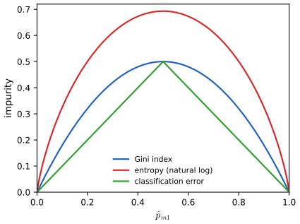
Exercise 3: Gini index, entropy (natural logarithm) and classification error for two classes. Code: fig_ex_8_3. Download: PDF · SVGExercise 8.4. (a) Sketch the tree that corresponds to the partition in the left panel of Figure 8.14 (the numbers are the means of \(Y\)). (b) Draw the partition that corresponds to the tree in the right panel.
Solution
(a) The root splits on \(X_1<1\); the right side (\(X_1\ge1\)) is a leaf with mean 5. On the left, \(X_2<1\): above it (\(X_2\ge1\)) a leaf with 15. Below, \(X_1<0\): a leaf with 3 on its left; on its right, \(X_2<0\) separates 10 (below) from 0 (above).
(b) The root splits at \(X_2=1\). Below it, \(X_1<1\) gives \(-1.80\) (left) and \(0.63\) (right). Above it, \(X_2<2\): between \(X_2=1\) and 2, \(X_1<0\) gives \(-1.06\) and \(0.21\); above \(X_2=2\) the mean is \(2.49\).
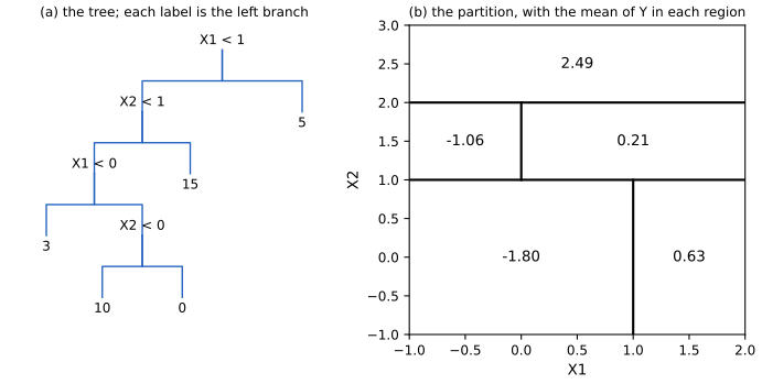
Exercise 4: (a) the tree for the left panel of Figure 8.14; (b) the partition for its right panel. Code: fig_ex_8_4. Download: PDF · SVGExercise 8.5. Ten bootstrapped trees give \(\Pr(\text{Red}\given X)=\) 0.1, 0.15, 0.2, 0.2, 0.55, 0.6, 0.6, 0.65, 0.7, 0.75. What is the class by majority vote, and by the average probability?
Solution
Majority vote: six of the ten trees give a probability above 0.5 and vote Red, four vote Green: Red. Average probability: \[ (0.1+0.15+0.2+0.2+0.55+0.6+0.6+0.65+0.7+0.75)/10=4.5/10=0.45<0.5 \]: Green. The two rules disagree because the Green votes are confident (0.1 to 0.2) and the Red votes are not (0.55 to 0.75). Averaging probabilities uses that information and tends to give better-calibrated probabilities; scikit-learn's random forest averages probabilities, R's
randomForest()counts votes.Exercise 8.6. Explain in detail the algorithm used to fit a regression tree.
Solution
1. Grow. Start with all training observations in one node. For every input \(X_j\) and every cutpoint \(s\) between two adjacent distinct values, compute the RSS (8.3) of the two halves \(\{X_j<s\}\), \(\{X_j\ge s\}\), each predicted by its mean; one sorted pass per input suffices (Result 8.1). Make the best split, then repeat within each child, and so on, until a stopping rule holds (too few observations in a node, children too small, or too small a decrease in RSS). 2. Prune. For each \(\alpha\ge0\) the subtree minimising \(\RSS(T)+\alpha|T|\) (8.4) is found by weakest-link pruning, which collapses, one at a time, the internal node with the smallest decrease in RSS per leaf removed; this gives a nested sequence of subtrees and the \(\alpha\) at which each appears (Result 8.2). 3. Choose \(\alpha\) by \(K\)-fold cross-validation: for each fold, grow and prune on the other folds and compute the test MSE on this fold at each \(\alpha\); average and take the \(\alpha\) with the smallest CV error. 4. Return the subtree of the full-data sequence for that \(\alpha\). 5. Predict a new \(x\) by dropping it down the tree to a leaf and returning the leaf's mean (Algorithm 8.1).
Exercise 8.7. Boston data: plot the test error of random forests for a range of
mtry(\(m\)) and of numbers of trees, in the style of Figure 8.10, and describe the results.Solution
R
# Exercise 7: random forests on the Boston data for several mtry, test MSE against the number of trees
p <- 12
ex7 <- sapply(c(12, 6, 3), function(m) {
  set.seed(1)
  randomForest(Boston[train, -13], Boston$medv[train], xtest = Boston[-train, -13],
               ytest = Boston$medv[-train], mtry = m, ntree = 500)$test$mse
})
open_svg("lab-r-ex7", 6, 4)
matplot(1:500, ex7, type = "l", lty = 1, col = c("orange", "blue", "darkgreen"), xlab = "Number of trees",
        ylab = "Test MSE", ylim = c(10, 30))
legend("topright", c("m = p = 12", "m = p/2 = 6", "m = 3"), col = c("orange", "blue", "darkgreen"), lty = 1)
invisible(dev.off())
cat("Exercise 7: test MSE after 500 trees, m = 12, 6, 3:", round(ex7[500, ], 3), "\n")
keep("ex7_500", ex7[500, ])
Python
    # Exercise 7: random forests on the Boston data for several m, test MSE against the number of trees
    ex7 = {}
    for m in (12, 6, 3):
        P = Forest(m, ntree=500, seed=7).fit(Xb[train], yb[train]).tree_predictions(Xb[test])
        ex7[m] = ((np.cumsum(P, 0) / np.arange(1, 501)[:, None] - yb[test]) ** 2).mean(1)
    fig, ax = plt.subplots(figsize=(6, 4))
    for m, col, lab in ((12, "orange", "m = p = 12"), (6, "blue", "m = p/2 = 6"), (3, "darkgreen", "m = 3")):
        ax.plot(np.arange(1, 501), ex7[m], color=col, label=lab)
    ax.set(xlabel="Number of trees", ylabel="Test MSE", ylim=(10, 30))
    ax.legend()
    common.savefig(fig, 8, "lab-py-ex7", formats=("svg",))
    print("Exercise 7: test MSE after 500 trees, m = 12, 6, 3:", [round(ex7[m][-1], 3) for m in (12, 6, 3)])
    keep("ex7_500", [ex7[m][-1] for m in (12, 6, 3)])
test MSE after 500 trees, m = 12, 6, 3: R 23.54 20.21 18.49 Python 23.03 19.30 18.55
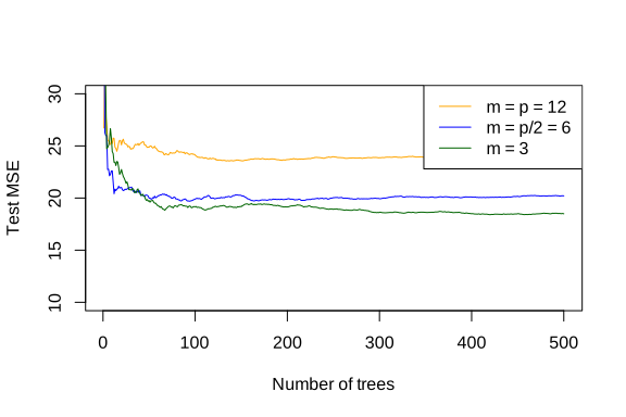
R: lab-r-ex7.svg.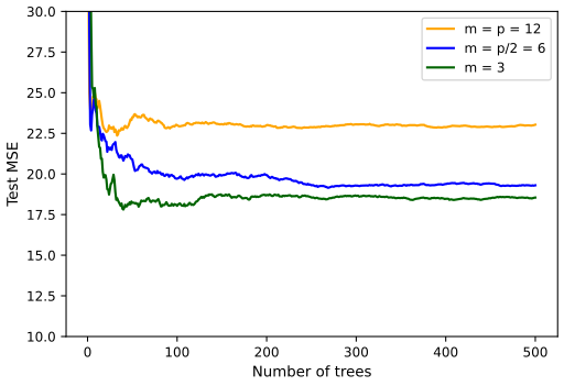
Python: lab-py-ex7.svg.In both languages the test error drops quickly over the first 30 to 50 trees and is flat after about 100: more trees do not overfit. Smaller \(m\) is better on this split: \(m=3\approx\sqrt p\) beats \(m=6\), which beats bagging (\(m=12\)), by several units of MSE, larger than the differences between the two languages' random numbers. The strong inputs rm and lstat dominate the bagged trees, and decorrelating them pays (Filling the gap 8.8).
Exercise 8.8. Carseats, Sales as a quantitative response: (a) split into training and test sets; (b) fit a regression tree, plot and interpret it, and give its test MSE; (c) use cross-validation to choose the tree size: does pruning help? (d) bagging, with test MSE and importance; (e) random forests, with the effect of \(m\); (f) BART.
Solution
R
# Exercise 8: regression trees and ensembles for Sales in Carseats
Carseats$High <- NULL
set.seed(1)
tr8 <- sample(1:nrow(Carseats), nrow(Carseats) / 2)
te8 <- Carseats[-tr8, ]
t8 <- tree(Sales ~ ., Carseats, subset = tr8)
print(summary(t8))
open_svg("lab-r-ex8-tree", 10, 6)
plot(t8); text(t8, pretty = 0, cex = 0.55)
invisible(dev.off())
cat("Exercise 8(b): tree with", summary(t8)$size, "leaves, test MSE", mse(predict(t8, te8), te8$Sales), "\n")
keep("ex8_size", summary(t8)$size); keep("ex8_tree_mse", mse(predict(t8, te8), te8$Sales))
cv8 <- cv.tree(t8)
print(cv8)
best8 <- cv8$size[which.min(cv8$dev)]
p8 <- prune.tree(t8, best = best8)
cat("Exercise 8(c): CV picks", best8, "leaves; pruned test MSE", mse(predict(p8, te8), te8$Sales), "\n")
keep("ex8_cv_dev", cv8$dev); keep("ex8_best", best8); keep("ex8_prune_mse", mse(predict(p8, te8), te8$Sales))
set.seed(1)
bag8 <- randomForest(Sales ~ ., data = Carseats, subset = tr8, mtry = 10, importance = TRUE)
cat("Exercise 8(d): bagging test MSE", mse(predict(bag8, te8), te8$Sales), "\n")
print(round(importance(bag8), 2))
keep("ex8_bag_mse", mse(predict(bag8, te8), te8$Sales))
rf8 <- sapply(1:10, function(m) {
  set.seed(1)
  mse(predict(randomForest(Sales ~ ., data = Carseats, subset = tr8, mtry = m), te8), te8$Sales)
})
cat("Exercise 8(e): random forest test MSE for m = 1..10:", round(rf8, 3), "\n")
keep("ex8_rf_mse", rf8)
set.seed(1)
quiet(bart8 <- gbart(Carseats[tr8, -1], Carseats$Sales[tr8], x.test = Carseats[-tr8, -1]))
cat("Exercise 8(f): BART test MSE", mse(bart8$yhat.test.mean, te8$Sales), "\n")
keep("ex8_bart_mse", mse(bart8$yhat.test.mean, te8$Sales))
lm8 <- lm(Sales ~ ., data = Carseats, subset = tr8)          # for comparison: least squares
cat("Exercise 8: least squares test MSE", mse(predict(lm8, te8), te8$Sales), "\n")
keep("ex8_lm_mse", mse(predict(lm8, te8), te8$Sales))
Python
    # Exercise 8: regression trees and ensembles for Sales in Carseats
    Car = factors(common.isl_data("Carseats"))
    rng = RRandom(1)
    tr8 = rng.sample(len(Car), len(Car) // 2) - 1
    te8 = np.setdiff1d(np.arange(len(Car)), tr8)
    X8, y8 = Car.drop(columns="Sales"), Car["Sales"]
    t8 = RTree().fit(X8.iloc[tr8], y8.iloc[tr8])
    print_summary(t8)
    fig, ax = plt.subplots(figsize=(11, 6))
    draw_tree(t8, ax, digits=2, fontsize=6.5)
    common.savefig(fig, 8, "lab-py-ex8-tree", formats=("svg",))
    m8 = mse(t8.predict(X8.iloc[te8]), y8.iloc[te8])
    print("Exercise 8(b): tree with %d leaves, test MSE %.5f" % (len(t8.leaves()), m8))
    keep("ex8_size", len(t8.leaves())); keep("ex8_tree_mse", m8)
    cv8 = cv_tree(t8, X8.iloc[tr8], y8.iloc[tr8], rng.sample(10, len(tr8), replace=True))
    best8 = int(cv8["size"][np.argmin(cv8["dev"])])
    p8 = t8.prune(best8)
    print("Exercise 8(c): CV deviance", np.round(cv8["dev"], 3), "picks", best8, "leaves; pruned test MSE %.5f"
          % mse(p8.predict(X8.iloc[te8]), y8.iloc[te8]))
    keep("ex8_cv_dev", cv8["dev"]); keep("ex8_best", best8); keep("ex8_prune_mse", mse(p8.predict(X8.iloc[te8]), y8.iloc[te8]))
    D8 = dummies(X8)                                     # scikit-learn needs numbers: 0/1 columns for the factors
    Z8, Zn = D8.to_numpy(), list(D8.columns)
    bag8 = Forest(Z8.shape[1], ntree=500, seed=8).fit(Z8[tr8], y8.iloc[tr8])
    print("Exercise 8(d): bagging test MSE %.5f" % mse(bag8.predict(Z8[te8]), y8.iloc[te8]))
    print(bag8.importance().set_index(pd.Index(Zn)).round(2))
    keep("ex8_bag_mse", mse(bag8.predict(Z8[te8]), y8.iloc[te8]))
    rf8 = [mse(Forest(m, ntree=500, seed=8).fit(Z8[tr8], y8.iloc[tr8]).predict(Z8[te8]), y8.iloc[te8])
           for m in range(1, Z8.shape[1] + 1)]
    print("Exercise 8(e): random forest test MSE for m = 1..%d:" % Z8.shape[1], np.round(rf8, 3))
    keep("ex8_rf_mse", rf8)
    F8 = dummies(X8, drop_first=False).to_numpy()
    bart8 = BART(seed=8).fit(F8[tr8], y8.iloc[tr8], F8[te8])
    print("Exercise 8(f): BART test MSE %.5f" % mse(bart8.yhat_test.mean(0), y8.iloc[te8]))
    keep("ex8_bart_mse", mse(bart8.yhat_test.mean(0), y8.iloc[te8]))
    A8 = np.column_stack([np.ones(len(Z8)), Z8])            # for comparison: least squares
    lm8 = mse(A8[te8] @ np.linalg.lstsq(A8[tr8], y8.iloc[tr8], rcond=None)[0], y8.iloc[te8])
    print("Exercise 8: least squares test MSE %.5f" % lm8)
    keep("ex8_lm_mse", lm8)
Carseats Sales, 200/200 split R Python (b) regression tree: leaves; test MSE 18; 4.922 18; 4.922 (c) CV deviance, sizes 18, 17, 16, 15, ... 831.3, 852.4, 868.7, 862.3, ... identical (d) bagging (all inputs), test MSE 2.605 2.687 (e) random forest, \(m=1,2,3,4,6,10\) 4.80, 3.52, 3.01, 2.84, 2.68, 2.59 4.61, 3.72, 3.17, 2.96, 2.76, 2.68 (f) BART, test MSE 1.451 1.457 least squares, all inputs, test MSE 0.988 0.988 (b) The tree (18 leaves) splits first on ShelveLoc (Good against Bad and Medium) and then mostly on Price, with Age, Advertising and CompPrice lower down: better shelf locations and lower prices sell more. Test MSE 4.92, i.e. about 2.2 thousand units in root-mean-square error.
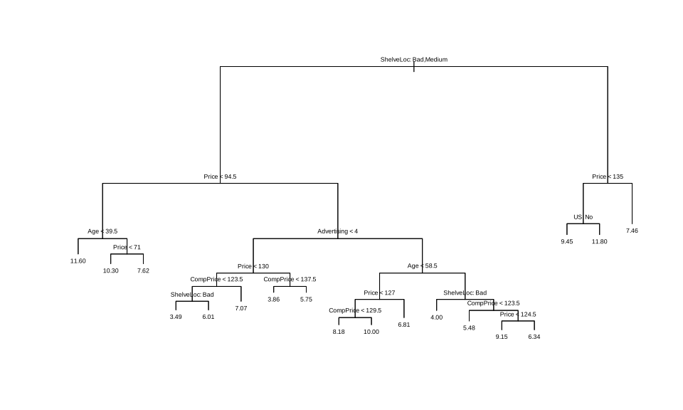
R: lab-r-ex8-tree.svg.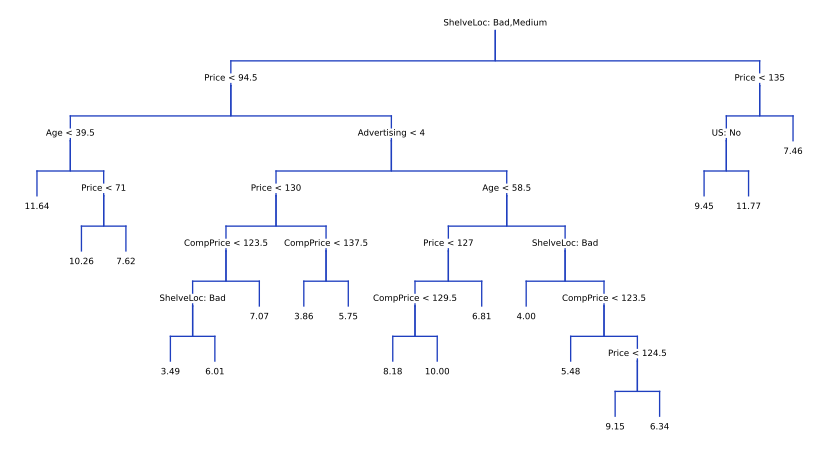
Python: lab-py-ex8-tree.svg.(c) Cross-validation picks the full 18-leaf tree, so pruning does not improve the test MSE here. (d) Bagging halves the test MSE, to 2.6. Both importance measures put Price and ShelveLoc far ahead, then CompPrice, Age and Advertising; Population, Education and Urban hardly matter (Population's %IncMSE is even negative: permuting it changes nothing beyond noise). (e) The test MSE falls steadily as \(m\) grows, from 4.8 at \(m=1\) to 2.6 at \(m=10\): with only two strong inputs, a split that cannot see Price or ShelveLoc is a wasted split, so here bagging (\(m=p\)) is as good as any forest. (f) BART is the best of the tree methods by far, 1.45: a sum of small trees captures a smooth, nearly additive dependence much better than deep trees do. But least squares with all inputs does better still (test MSE 0.988, identical in both languages): Sales is close to linear in these inputs, the situation of the top row of Figure 8.7, where a linear model beats trees.
Exercise 8.9. OJ data: (a) a training set of 800 purchases; (b) a tree for Purchase, its training error and size; (c) interpret one leaf; (d) plot and interpret the tree; (e) test confusion matrix and error; (f)–(h) cross-validation over the size; (i) prune to the best size (or 5 leaves); (j)–(k) compare training and test errors of the pruned and unpruned trees.
Solution
R
# Exercise 9: classification trees on the OJ data
set.seed(1)
tr9 <- sample(1:nrow(OJ), 800)
t9 <- tree(Purchase ~ ., OJ, subset = tr9)
print(summary(t9))
print(t9)
open_svg("lab-r-ex9-tree", 7, 4.5)
plot(t9); text(t9, pretty = 0, cex = 0.7)
invisible(dev.off())
pred9 <- predict(t9, OJ[-tr9, ], type = "class")
print(table(pred9, OJ$Purchase[-tr9]))
keep("ex9_size", summary(t9)$size); keep("ex9_train_err", summary(t9)$misclass[1] / 800)
keep("ex9_test_err", mean(pred9 != OJ$Purchase[-tr9]))
cv9 <- cv.tree(t9, FUN = prune.misclass)
print(cv9)
keep("ex9_cv_size", cv9$size); keep("ex9_cv_dev", cv9$dev)
open_svg("lab-r-ex9-cv", 4.5, 3.6)
plot(cv9$size, cv9$dev / 800, type = "b", xlab = "Tree size", ylab = "CV classification error")
invisible(dev.off())
best9 <- cv9$size[which.min(cv9$dev)]
if (best9 == max(cv9$size)) best9 <- 5           # CV keeps the full tree: prune to five leaves instead
p9 <- prune.misclass(t9, best = best9)
pred9p <- predict(p9, OJ[-tr9, ], type = "class")
cat("Exercise 9: pruned to", best9, "leaves; training error", summary(p9)$misclass[1] / 800,
    "test error", mean(pred9p != OJ$Purchase[-tr9]), "\n")
keep("ex9_best", best9); keep("ex9_prune_train_err", summary(p9)$misclass[1] / 800)
keep("ex9_prune_test_err", mean(pred9p != OJ$Purchase[-tr9]))
Python
    # Exercise 9: classification trees on the OJ data
    OJ = factors(common.isl_data("OJ"))
    rng = RRandom(1)
    tr9 = rng.sample(len(OJ), 800) - 1
    te9 = np.setdiff1d(np.arange(len(OJ)), tr9)
    X9, y9 = OJ.drop(columns="Purchase"), OJ["Purchase"]
    t9 = RTree().fit(X9.iloc[tr9], y9.iloc[tr9])
    s9 = print_summary(t9)
    print(t9.text())
    pred9 = t9.predict(X9.iloc[te9], "class", rng=rng)
    print(pd.crosstab(pd.Series(pred9, name="pred"), pd.Series(y9.iloc[te9].astype(str).to_numpy(), name="truth")))
    keep("ex9_size", s9["size"]); keep("ex9_train_err", s9["error_rate"])
    keep("ex9_test_err", np.mean(pred9 != y9.iloc[te9].astype(str).to_numpy()))
    cv9 = cv_tree(t9, X9.iloc[tr9], y9.iloc[tr9], rng.sample(10, 800, replace=True), method="misclass")
    print("Exercise 9(f): size", cv9["size"], "CV errors", cv9["dev"])
    keep("ex9_cv_size", cv9["size"]); keep("ex9_cv_dev", cv9["dev"])
    best9 = int(cv9["size"][np.argmin(cv9["dev"])])
    if best9 == cv9["size"].max():
        best9 = 5                                        # CV keeps the full tree: prune to five leaves instead
    p9 = t9.prune(best9, method="misclass")
    pred9p = p9.predict(X9.iloc[te9], "class", rng=rng)
    e_tr, e_te = p9.summary()["error_rate"], np.mean(pred9p != y9.iloc[te9].astype(str).to_numpy())
    print("Exercise 9: pruned to %d leaves; training error %.4f, test error %.6f" % (best9, e_tr, e_te))
    keep("ex9_best", best9); keep("ex9_prune_train_err", e_tr); keep("ex9_prune_test_err", e_te)
1) root 800 1070.0 CH ( 0.6062 0.3937 ) 2) LoyalCH < 0.5036 365 442.0 MM ( 0.2932 0.7068 ) 4) LoyalCH < 0.280875 177 140.0 MM ( 0.1356 0.8644 ) 8) LoyalCH < 0.0356415 59 10.1 MM ( 0.0169 0.9831 ) * 9) LoyalCH > 0.0356415 118 116.0 MM ( 0.1949 0.8051 ) * 5) LoyalCH > 0.280875 188 258.0 MM ( 0.4415 0.5585 ) 10) PriceDiff < 0.05 79 84.8 MM ( 0.2278 0.7722 ) 20) SpecialCH < 0.5 64 52.0 MM ( 0.1406 0.8594 ) * 21) SpecialCH > 0.5 15 20.2 CH ( 0.6000 0.4000 ) * 11) PriceDiff > 0.05 109 147.0 CH ( 0.5963 0.4037 ) * 3) LoyalCH > 0.5036 435 338.0 CH ( 0.8690 0.1310 ) 6) LoyalCH < 0.764572 174 201.0 CH ( 0.7356 0.2644 ) 12) ListPriceDiff < 0.235 72 99.8 MM ( 0.5000 0.5000 ) 24) PctDiscMM < 0.196196 55 73.1 CH ( 0.6182 0.3818 ) * 25) PctDiscMM > 0.196196 17 12.3 MM ( 0.1176 0.8824 ) * 13) ListPriceDiff > 0.235 102 65.4 CH ( 0.9020 0.0980 ) * 7) LoyalCH > 0.764572 261 91.2 CH ( 0.9579 0.0421 ) * (R; Python prints the same tree)(b) Nine leaves; the tree uses LoyalCH, PriceDiff, SpecialCH, ListPriceDiff and PctDiscMM; training error 127/800 = 0.159 (residual mean deviance 0.743). (c) Leaf 8: the 59 customers with brand loyalty to Citrus Hill below 0.036; 98.3% of them bought Minute Maid, the leaf predicts MM, and its deviance (10.1) is small because it is nearly pure. (d) Loyalty to Citrus Hill is by far the most important input: the first three levels of the tree split on it; price differences and promotions only matter for customers with intermediate loyalty.
pred   CH  MM
  CH  160  38
  MM    8  64          test error 46/270 = 0.170 (both languages)
size   9   8   7   4   2   1
CV   150 150 149 158 172 315 errors out of 800 (both languages)
(e) Test error 0.170. (f)–(h) Ten-fold cross-validation is lowest at 7 leaves (149 errors), with 8 and 9 leaves one error behind: the size hardly matters between 7 and 9, while 1 leaf (always CH) makes 315 errors. (i) The pruned tree has 7 leaves. (j) Its training error, 130/800 = 0.1625, is higher than the unpruned tree's 0.159, as it must be (a subtree cannot fit the training data better). (k) Its test error, 44/270 = 0.163, is lower than the unpruned tree's 0.170, by two customers.
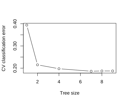
Exercise 9(g), R: CV classification error against tree size, lab-r-ex9-cv.svg.Exercise 8.10. Hitters, log(Salary), first 200 players for training: (c)–(d) boosting with 1000 trees over a range of \(\lambda\), with training and test MSE; (e) compare with two methods of Chapters 3 and 6; (f) the most important inputs; (g) bagging.
Solution
R
# Exercise 10: boosting for log(Salary) in the Hitters data, first 200 players for training
H <- na.omit(Hitters)
H$Salary <- log(H$Salary)
Htr <- H[1:200, ]; Hte <- H[-(1:200), ]
lams <- c(0.001, 0.002, 0.005, 0.01, 0.02, 0.05, 0.1, 0.2, 0.3, 0.5, 0.7, 1)
ex10 <- t(sapply(lams, function(l) {
  set.seed(1)
  b <- gbm(Salary ~ ., data = Htr, distribution = "gaussian", n.trees = 1000, shrinkage = l)
  c(train = mse(predict(b, Htr, n.trees = 1000), Htr$Salary), test = mse(predict(b, Hte, n.trees = 1000), Hte$Salary))
}))
print(cbind(lambda = lams, ex10))
keep("ex10_train", ex10[, 1]); keep("ex10_test", ex10[, 2])
open_svg("lab-r-ex10", 8, 3.6)
par(mfrow = c(1, 2))
plot(lams, ex10[, 1], log = "x", type = "b", xlab = "shrinkage", ylab = "training MSE")
plot(lams, ex10[, 2], log = "x", type = "b", xlab = "shrinkage", ylab = "test MSE")
invisible(dev.off())
lm10 <- lm(Salary ~ ., data = Htr)
Xtr10 <- model.matrix(Salary ~ ., Htr)[, -1]; Xte10 <- model.matrix(Salary ~ ., Hte)[, -1]
# ridge regression with lambda chosen by exact leave-one-out (standardised inputs, closed form)
mu <- colMeans(Xtr10); sdv <- apply(Xtr10, 2, sd)
Z <- scale(Xtr10, mu, sdv); Zte <- scale(Xte10, mu, sdv); yc <- Htr$Salary - mean(Htr$Salary)
loo <- sapply(10^seq(-2, 4, length.out = 121), function(l) {
  Hm <- Z %*% solve(crossprod(Z) + l * diag(ncol(Z)), t(Z))
  mean(((yc - Hm %*% yc) / (1 - diag(Hm) - 1 / nrow(Z)))^2)
})
lbest <- 10^seq(-2, 4, length.out = 121)[which.min(loo)]
br <- solve(crossprod(Z) + lbest * diag(ncol(Z)), crossprod(Z, yc))
cat("Exercise 10(e): test MSE: boosting (shrinkage 0.01)", ex10[lams == 0.01, 2], " least squares",
    mse(predict(lm10, Hte), Hte$Salary), " ridge (lambda", signif(lbest, 4), ")",
    mse(mean(Htr$Salary) + Zte %*% br, Hte$Salary), "\n")
keep("ex10_lm_mse", mse(predict(lm10, Hte), Hte$Salary)); keep("ex10_ridge_lambda", lbest)
keep("ex10_ridge_mse", mse(mean(Htr$Salary) + Zte %*% br, Hte$Salary))
set.seed(1)
b10 <- gbm(Salary ~ ., data = Htr, distribution = "gaussian", n.trees = 1000, shrinkage = 0.01)
print(head(summary(b10, plotit = FALSE), 5))
set.seed(1)
bag10 <- randomForest(Salary ~ ., data = Htr, mtry = 19)
cat("Exercise 10(g): bagging test MSE", mse(predict(bag10, Hte), Hte$Salary), "\n")
keep("ex10_bag_mse", mse(predict(bag10, Hte), Hte$Salary))
Python
    # Exercise 10: boosting for log(Salary) in the Hitters data, first 200 players for training
    H = factors(common.isl_data("Hitters")).dropna().reset_index(drop=True)
    H["Salary"] = np.log(H["Salary"])
    XH = dummies(H.drop(columns="Salary"))
    Xtr, Xte = XH.iloc[:200].to_numpy(), XH.iloc[200:].to_numpy()
    ytr, yte = H["Salary"].iloc[:200].to_numpy(), H["Salary"].iloc[200:].to_numpy()
    lams = [0.001, 0.002, 0.005, 0.01, 0.02, 0.05, 0.1, 0.2, 0.3, 0.5, 0.7, 1]
    ex10 = []
    for lam in lams:
        g = gbm_like(1000, depth=1, shrinkage=lam, seed=10).fit(Xtr, ytr)
        ex10.append((mse(g.predict(Xtr), ytr), mse(g.predict(Xte), yte)))
    ex10 = np.array(ex10)
    print(pd.DataFrame(ex10, index=lams, columns=["train", "test"]).round(5))
    keep("ex10_train", ex10[:, 0]); keep("ex10_test", ex10[:, 1])
    fig, ax = plt.subplots(1, 2, figsize=(8, 3.6))
    for a, k, lab in ((ax[0], 0, "training MSE"), (ax[1], 1, "test MSE")):
        a.plot(lams, ex10[:, k], "o-", ms=4)
        a.set(xscale="log", xlabel="shrinkage", ylabel=lab)
    common.savefig(fig, 8, "lab-py-ex10", formats=("svg",))
    A = np.column_stack([np.ones(200), Xtr])
    beta = np.linalg.lstsq(A, ytr, rcond=None)[0]
    lm_mse = mse(np.column_stack([np.ones(len(yte)), Xte]) @ beta, yte)
    mu, sd = Xtr.mean(0), Xtr.std(0, ddof=1)             # ridge with exact leave-one-out, as in the R lab
    Z, Zte, yc = (Xtr - mu) / sd, (Xte - mu) / sd, ytr - ytr.mean()
    grid = 10 ** np.linspace(-2, 4, 121)
    loo = []
    for l in grid:
        Hm = Z @ np.linalg.solve(Z.T @ Z + l * np.eye(Z.shape[1]), Z.T)
        loo.append(np.mean(((yc - Hm @ yc) / (1 - np.diag(Hm) - 1 / len(yc))) ** 2))
    lbest = grid[int(np.argmin(loo))]
    br = np.linalg.solve(Z.T @ Z + lbest * np.eye(Z.shape[1]), Z.T @ yc)
    ridge_mse = mse(ytr.mean() + Zte @ br, yte)
    print("Exercise 10(e): test MSE: boosting (shrinkage 0.01) %.6f, least squares %.6f, ridge (lambda %.4g) %.6f"
          % (ex10[lams.index(0.01), 1], lm_mse, lbest, ridge_mse))
    keep("ex10_lm_mse", lm_mse); keep("ex10_ridge_lambda", lbest); keep("ex10_ridge_mse", ridge_mse)
    g = gbm_like(1000, depth=1, shrinkage=0.01, seed=10).fit(Xtr, ytr)
    print(pd.Series(100 * g.feature_importances_, XH.columns).sort_values(ascending=False).head(5).round(3))
    bag10 = Forest(Xtr.shape[1], ntree=500, seed=10).fit(Xtr, ytr)
    print("Exercise 10(g): bagging test MSE %.6f" % mse(bag10.predict(Xte), yte))
    keep("ex10_bag_mse", mse(bag10.predict(Xte), yte))
\(\lambda\) 0.001 0.005 0.01 0.02 0.05 0.1 0.2 0.5 1 training, R 0.361 0.171 0.140 0.113 0.080 0.051 0.025 0.005 0.001 test, R 0.338 0.289 0.280 0.266 0.265 0.253 0.301 0.326 0.563 test, Python 0.336 0.290 0.277 0.265 0.261 0.287 0.272 0.330 0.564 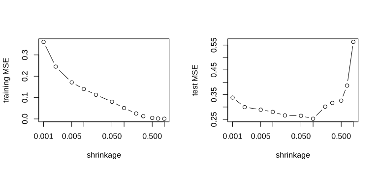
R: lab-r-ex10.svg.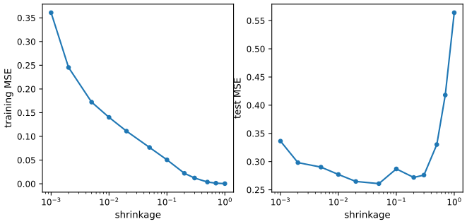
Python: lab-py-ex10.svg.(c)–(d) With 1000 stumps the training MSE falls steadily as \(\lambda\) grows (to nearly 0 at \(\lambda=1\)), while the test MSE is U-shaped: too small a \(\lambda\) has not learned enough in 1000 trees, too large a \(\lambda\) overfits. The minimum, about 0.25–0.26, lies between \(\lambda=0.02\) and 0.1; the exact place moves with the random half-samples (R and Python differ there). (e) Least squares on all 19 inputs has test MSE 0.492 and ridge regression with \(\lambda\) chosen by exact leave-one-out (\(\lambda=4.47\) on standardised inputs) 0.461, identical in both languages; boosting, at 0.28 for \(\lambda=0.01\), is far better, because log salary depends on career length in a strongly non-linear way. (f) The career totals dominate: CAtBat (27% of the relative influence in R, 25% in Python), then CHits, CRBI, CWalks and CRuns. (g) Bagging does even better than boosting here: test MSE 0.230 in both languages.
Exercise 8.11. Caravan, first 1000 customers for training: (b) boosting with 1000 trees and shrinkage 0.01, and the most important inputs; (c) predict a purchase when the estimated probability exceeds 20%: what fraction of the predicted buyers buy, compared with KNN and logistic regression?
Solution
R
# Exercise 11: boosting on the Caravan data, first 1000 customers for training
Cv <- Caravan
Cv$Purchase <- as.numeric(Cv$Purchase == "Yes")
Ctr <- Cv[1:1000, ]; Cte <- Cv[-(1:1000), ]
set.seed(1)
b11 <- suppressWarnings(gbm(Purchase ~ ., data = Ctr, distribution = "bernoulli", n.trees = 1000, shrinkage = 0.01))
print(head(summary(b11, plotit = FALSE), 6))
p11 <- predict(b11, Cte, n.trees = 1000, type = "response")
print(table(predicted = p11 > 0.2, purchase = Cte$Purchase))
keep("ex11_boost_prec", sum(p11 > 0.2 & Cte$Purchase == 1) / sum(p11 > 0.2)); keep("ex11_boost_npred", sum(p11 > 0.2))
lg11 <- suppressWarnings(glm(Purchase ~ ., data = Ctr, family = binomial))
q11 <- suppressWarnings(predict(lg11, Cte, type = "response"))
print(table(predicted = q11 > 0.2, purchase = Cte$Purchase))
keep("ex11_logit_prec", sum(q11 > 0.2 & Cte$Purchase == 1) / sum(q11 > 0.2)); keep("ex11_logit_npred", sum(q11 > 0.2))
Xs <- scale(Caravan[, -86])
set.seed(1)
k11 <- knn(Xs[1:1000, ], Xs[-(1:1000), ], Caravan$Purchase[1:1000], k = 5)
print(table(predicted = k11, purchase = Cte$Purchase))
keep("ex11_knn_prec", sum(k11 == "Yes" & Cte$Purchase == 1) / sum(k11 == "Yes"))
Python
    # Exercise 11: boosting on the Caravan data, first 1000 customers for training
    Cv = common.isl_data("Caravan")
    yC = (Cv["Purchase"] == "Yes").to_numpy(int)
    XC = Cv.drop(columns="Purchase").to_numpy(float)
    g11 = gbm_like(1000, depth=1, shrinkage=0.01, classification=True, seed=11).fit(XC[:1000], yC[:1000])
    print(pd.Series(100 * g11.feature_importances_, Cv.columns[:-1]).sort_values(ascending=False).head(6).round(3))
    p11 = g11.predict_proba(XC[1000:])[:, 1]
    print(pd.crosstab(pd.Series(p11 > 0.2, name="predicted"), pd.Series(yC[1000:], name="purchase")))
    keep("ex11_boost_prec", np.mean(yC[1000:][p11 > 0.2])); keep("ex11_boost_npred", int((p11 > 0.2).sum()))
    lg = sm.GLM(yC[:1000], sm.add_constant(XC[:1000]), family=sm.families.Binomial()).fit()
    q11 = lg.predict(sm.add_constant(XC[1000:]))
    print(pd.crosstab(pd.Series(q11 > 0.2, name="predicted"), pd.Series(yC[1000:], name="purchase")))
    keep("ex11_logit_prec", np.mean(yC[1000:][q11 > 0.2])); keep("ex11_logit_npred", int((q11 > 0.2).sum()))
    XCs = (XC - XC.mean(0)) / XC.std(0, ddof=1)
    k11 = KNeighborsClassifier(5).fit(XCs[:1000], yC[:1000]).predict(XCs[1000:])
    print(pd.crosstab(pd.Series(k11, name="predicted"), pd.Series(yC[1000:], name="purchase")))
    keep("ex11_knn_prec", np.mean(yC[1000:][k11 == 1]))
Caravan, 4822 test customers (6.0% buy) R: predicted buyers; of them buy Python boosting, \(\hat p>0.2\) 156; 33 (21.2%) 158; 33 (20.9%) logistic regression, \(\hat p>0.2\) 408; 58 (14.2%) 407; 58 (14.3%) KNN, \(K=5\), standardised inputs 37; 10 (27.0%) 37; 10 (27.0%) (b) The most influential inputs are PPERSAUT (contribution to car policies), MKOOPKLA (purchasing-power class), MOPLHOOG (higher education), MBERMIDD and PBRAND. (c) About one in five customers predicted to buy does buy with boosting, against one in seven for logistic regression at the same threshold and a base rate of one in seventeen. KNN with \(K=5\) is more precise (27%) but finds far fewer buyers (10 against 33). The logistic fit on 1000 customers with 85 inputs is unstable (R warns that some fitted probabilities are 0 or 1), which costs it one customer of difference between the languages; see Section 4.7.6 for the same comparison with the roles of the two sets exchanged.
Exercise 8.12. Apply boosting, bagging, random forests and BART to a data set of your choice and compare them with a simple method.
Solution
The Auto data: mpg from cylinders, displacement, horsepower, weight, acceleration, year and origin, on a random half of the 392 cars.
R
# Exercise 12: the Auto data, mpg from the seven other numeric variables
A <- Auto[, 1:8]
set.seed(1)
tr12 <- sample(1:nrow(A), nrow(A) / 2)
lm12 <- lm(mpg ~ ., A, subset = tr12)
set.seed(1); bag12 <- randomForest(mpg ~ ., A, subset = tr12, mtry = 7)
set.seed(1); rf12 <- randomForest(mpg ~ ., A, subset = tr12)
set.seed(1); gb12 <- gbm(mpg ~ ., data = A[tr12, ], distribution = "gaussian", n.trees = 2000,
                         interaction.depth = 2, shrinkage = 0.01)
set.seed(1); quiet(bt12 <- gbart(A[tr12, -1], A$mpg[tr12], x.test = A[-tr12, -1]))
ex12 <- c(lm = mse(predict(lm12, A[-tr12, ]), A$mpg[-tr12]), bagging = mse(predict(bag12, A[-tr12, ]), A$mpg[-tr12]),
          forest = mse(predict(rf12, A[-tr12, ]), A$mpg[-tr12]),
          boosting = mse(predict(gb12, A[-tr12, ], n.trees = 2000), A$mpg[-tr12]),
          BART = mse(bt12$yhat.test.mean, A$mpg[-tr12]))
print(round(ex12, 3))
keep("ex12", ex12)
Python
    # Exercise 12: the Auto data, mpg from the seven other numeric variables
    Au = common.isl_data("Auto", na_values="?").dropna().reset_index(drop=True)
    XA, yA = Au.iloc[:, 1:8].to_numpy(float), Au["mpg"].to_numpy(float)
    tr12 = RRandom(1).sample(len(yA), len(yA) // 2) - 1
    te12 = np.setdiff1d(np.arange(len(yA)), tr12)
    A1 = np.column_stack([np.ones(len(yA)), XA])
    b12 = np.linalg.lstsq(A1[tr12], yA[tr12], rcond=None)[0]
    ex12 = {"lm": mse(A1[te12] @ b12, yA[te12]),
            "bagging": mse(Forest(7, seed=12).fit(XA[tr12], yA[tr12]).predict(XA[te12]), yA[te12]),
            "forest": mse(Forest(2, seed=12).fit(XA[tr12], yA[tr12]).predict(XA[te12]), yA[te12]),
            "boosting": mse(gbm_like(2000, depth=2, shrinkage=0.01, seed=12).fit(XA[tr12], yA[tr12]).predict(XA[te12]), yA[te12]),
            "BART": mse(BART(seed=12).fit(XA[tr12], yA[tr12], XA[te12]).yhat_test.mean(0), yA[te12])}
    print("Exercise 12: test MSE", {k: round(v, 3) for k, v in ex12.items()})
    keep("ex12", list(ex12.values()))
test MSE least squares bagging random forest boosting BART R 9.878 7.000 6.935 7.533 6.633 Python 9.878 6.864 6.944 7.313 6.606
All four ensembles beat least squares (test MSE 9.88, identical in both languages) by about 25–33%, because mpg depends non-linearly on weight, horsepower and year and the inputs interact. The ensembles are within about 1 of one another, with BART slightly ahead with its default settings and boosting (2000 trees of depth 2, \(\lambda=0.01\), not tuned) slightly behind; on 196 test cars these differences are not decisive.
Demonstrations for this chapter
Each demonstration runs in the browser on the book's data and links back to these notes. The ▶ Demo boxes above open them already set to the case under discussion.
| Demonstration | What you can see | Sections |
|---|---|---|
| Growing and pruning a regression tree on the Hitters data | The regions of the tree in the Years–Hits plane, the tree, the RSS (8.3) of every candidate cutpoint of any node, and the cost-complexity criterion (8.4) of every subtree of the weakest-link sequence. Presets: 1 the first split; 2 Figure 8.1; 3 the full tree; 4 the weakest link; 5 the root alone. | 8.1.1 |
| Bagging against a random forest on the Heart data | Test and out-of-bag error against the number of trees, the input of each tree's first split, and how alike the trees are, for any \(m\), number of trees and seed. Presets: 1 Figure 8.8; 2 \(m=p\); 3 \(m=1\); 4 few trees; 5 another seed. | 8.2.1, 8.2.2 |
| Boosting regression trees on the Hitters data | Algorithm 8.2 with any \(\lambda\), \(d\) and \(B\): training and test MSE along the path, the test MSE against \(\lambda\), and the additive functions built by stumps (or the relative influence for deeper trees). Presets: 1 Exercise 10; 2 \(\lambda=1\); 3 \(\lambda=0.001\); 4 \(d=4\); 5 starting at zero. | 8.2.3, Ex. 10 |
Related demonstrations in the graduate course: growing and pruning a classification tree on the spam data, bagging classification trees, the out-of-bag error of a random forest and gradient boosting with subsampling and robust losses.
References
- James, G., Witten, D., Hastie, T. and Tibshirani, R. (2021). An Introduction to Statistical Learning with Applications in R, 2nd edition. Springer, New York. Chapter 8, pp. 327–365. www.statlearning.com.
- James, G., Witten, D., Hastie, T., Tibshirani, R. and Taylor, J. (2023). An Introduction to Statistical Learning with Applications in Python. Springer, Cham. Chapter 8.
- Breiman, L. (1996). Bagging predictors. Machine Learning, 24, 123–140.
- Breiman, L. (2001). Random forests. Machine Learning, 45, 5–32.
- Breiman, L., Friedman, J., Olshen, R. and Stone, C. (1984). Classification and Regression Trees. Wadsworth, Belmont.
- Chipman, H. A., George, E. I. and McCulloch, R. E. (2010). BART: Bayesian additive regression trees. Annals of Applied Statistics, 4(1), 266–298.
- Fisher, W. D. (1958). On grouping for maximum homogeneity. Journal of the American Statistical Association, 53, 789–798.
- Friedman, J. H. (2001). Greedy function approximation: a gradient boosting machine. Annals of Statistics, 29, 1189–1232.
- Hastie, T., Tibshirani, R. and Friedman, J. (2009). The Elements of Statistical Learning, 2nd edition. Springer, New York. Chapters 8, 9, 10 and 15.
- Sparapani, R., Spanbauer, C. and McCulloch, R. (2021). Nonparametric machine learning and efficient computation with Bayesian additive regression trees: the BART R package. Journal of Statistical Software, 97(1), 1–66.
The numerical statements in the text (the trees and their pruning sequences, the agreement of the R and Python labs, the out-of-bag fraction, the impurity calculations, the boosting identities and the exercise results) were confirmed numerically.