Unsupervised Learning
With no response to predict, the questions change: is there an informative low-dimensional picture of the data, and are there subgroups among the observations? Principal components analysis answers the first. It finds the directions in which the data vary most, which are also the subspaces closest to the data, and it measures how much of the variation a few components capture. The same low-rank idea fills in missing entries of a data matrix (matrix completion, the engine of recommender systems). Clustering answers the second, by K-means, which partitions the data into a chosen number of groups, or by hierarchical clustering, which builds a tree of nested groups. The USArrests and NCI60 data run through the chapter, and the lab is shown in R and Python side by side.
Ch. 1 Introduction Ch. 2 Statistical learning Ch. 3 Linear regression Ch. 4 Classification Ch. 5 Resampling Ch. 6 Selection and regularization Ch. 7 Beyond linearity Ch. 8 Trees Ch. 9 SVMs Ch. 10 Deep learning Ch. 11 Survival analysis Ch. 12 Unsupervised learning Ch. 13 Multiple testing
How to read these notes
They follow the book. Sections carry the book's numbers (12.2, 12.4.1, ...), and every displayed equation that appears in the book carries the book's own number, e.g. \((12.10)\). Both editions share the text, the figures and the exercises of this chapter; they differ only in the lab (Section 12.5), which is shown here in both languages.
Filling the gaps. The book states that principal components come from an eigen decomposition "outside the scope of this book", that they solve the approximation problem (12.6) ("it can be shown"), and that the K-means and matrix-completion algorithms never increase their objectives. An orange Filling the gap box gives each complete argument at the level of a first course in linear algebra and statistics. The derivations start hidden: open one with its bar, or use the button below.
Figures and demonstrations. All 19 figures of the chapter are recomputed by the Python code, from the data or from documented simulations. The ▶ Demo boxes open an interactive demonstration already set to the case being discussed.
Main references
G. James, D. Witten, T. Hastie and R. Tibshirani, An Introduction to Statistical Learning with Applications in R, 2nd edition, Springer (2021), Chapter 12; and G. James, D. Witten, T. Hastie, R. Tibshirani and J. Taylor, An Introduction to Statistical Learning with Applications in Python, Springer (2023), Chapter 12. Book website, with the data sets: www.statlearning.com. Section, equation, figure and exercise numbers below refer to these books; "James et al. (2021)" means text shared by both editions.
The explanations, derivations, figures and code are my own; equations are cited by their numbers in the book.
Companion courses
This course is the applied, introductory companion of the graduate course Statistical Learning: Theory and Methods (Hastie, Tibshirani and Friedman 2009), whose Chapter 14 treats this chapter's methods in more depth (proximity matrices and dissimilarities, combinatorial clustering, K-means as coordinate descent, Gaussian mixtures as soft K-means, K-medoids, principal curves, spectral clustering and kernel, sparse and non-negative factorisations). The ▷ Deeper lines below point to the matching sections.
- Statistical Methods for Modern Biology (Holmes and Huber 2019): clustering, its dissimilarities, k-means, hierarchical clustering and how to choose the number of clusters, Chapter 5; principal components, the SVD, biplots and their scalings, Chapter 7.
- Bayesian and Probabilistic Machine Learning (Bishop 2006): PCA as maximum variance and as minimum error, with probabilistic PCA and factor analysis, Chapter 12; K-means as the limit of a Gaussian mixture fitted by EM, Section 9.1 and Section 9.3.2.
- Within this course: principal components regression, which uses the scores of this chapter as predictors, Section 6.3.1; and the NCI60 picture of Chapter 1.
The chapter at a glance
- 12.1 Without a response there is no test error to check against, so unsupervised learning is exploratory and its results are harder to validate.
- 12.2 The first principal component is the unit vector \(\bphi_1\) maximising the variance of \(\bX\bphi_1\): the top eigenvector of the covariance matrix, with variance its eigenvalue (Result 12.1). The first \(M\) components give the best rank-\(M\) approximation of the centred data (Result 12.2), the variance splits into explained and residual parts, and the PVEs sum to one (Result 12.3). The components depend on the units unless the variables are standardised, and each is unique only up to sign (Result 12.4).
- 12.3 Missing entries are imputed by Algorithm 12.1, which alternates a rank-\(M\) fit and a refill of the missing cells; each pass can only lower the error on the observed cells (Result 12.5).
- 12.4 K-means minimises the within-cluster variation, which equals twice the sum of squared distances to the cluster means (12.18); each step of Algorithm 12.2 can only lower it (Result 12.6). Hierarchical clustering fuses the two closest clusters again and again; the fusion height measures dissimilarity, but horizontal position in the dendrogram does not (Result 12.7). Complete, single and average linkage never produce inversions, centroid linkage can (Result 12.8). Cuts of one tree are nested; the best K-means clusters need not be (Result 12.9). Correlation-based distance is squared Euclidean distance between standardised profiles (Result 12.10).
- 12.5 The lab, in R and Python: PCA of USArrests, matrix completion written out, K-means and hierarchical clustering of simulated data, and PCA and clustering of the NCI60 cancer cell lines.
Notation. \(\bX\) is the \(n\times p\) data matrix with rows \(x_i\) (observations) and columns \(X_j\) (features), centred so that every column has mean zero. Its covariance matrix is \(\bS=\frac1n\bX^\T\bX\) with the book's divisor \(n\) in (12.8)–(12.9); R's prcomp() and scikit-learn's explained_variance_ divide by \(n-1\), which multiplies every variance by the same factor and changes nothing else. The singular value decomposition (SVD) is \(\bX=\bU\bD\bV^\T\), with orthonormal columns in \(\bU\) (\(n\times r\)) and \(\bV\) (\(p\times r\)), \(\bD=\diag(d_1\ge\dots\ge d_r\gt0)\), \(r=\rank\bX\). \(\|\cdot\|\) is the Euclidean (or, for matrices, Frobenius) norm.
Prerequisites. Chapter 6 of the book (principal components regression, Section 6.3.1), and the matrix algebra of eigenvalues and eigenvectors of a symmetric matrix; the gap boxes recall what is needed.
12.1 The Challenge of Unsupervised Learning
Section 12.1 In supervised learning we observe features \(X_1,\dots,X_p\) and a response \(Y\) on the same \(n\) observations, and the goal is to predict \(Y\). In unsupervised learning there is no \(Y\): only the features. The aims become descriptive: find an informative way to look at the data, and find subgroups among the observations (or among the variables). This chapter covers the two workhorses, principal components analysis (PCA), for visualisation and as a pre-processing step, and clustering, for discovering subgroups.
The difficulty is that there is no answer to check against. A supervised model can be judged by its error on observations it did not see (Chapter 5); a picture or a set of clusters cannot, because the "true" structure is unknown. Unsupervised learning is therefore usually part of an exploratory data analysis, and its results are hypotheses to be confirmed on new data. The applications are everywhere: subtypes of a cancer from gene expression, groups of shoppers with similar purchase histories, and recommendations built from the ratings of similar customers.
12.2 Principal Components Analysis
Section 12.2 Principal components were met in Section 6.3.1 as the predictors of principal components regression: a few linear combinations of many correlated variables that keep most of their variability. Here the same components are used on their own, without a response, to visualise data, to summarise them, and to impute missing values.
12.2.1 What Are Principal Components?
With \(p\) features there are \(\binom p2=p(p-1)/2\) scatter plots of pairs of them (45 for \(p=10\)), each showing a small part of the information. PCA looks instead for a few directions in feature space along which the observations vary the most, and plots the data in those directions.
Definition 12.1 (principal component loadings and scores) Section 12.2.1, (12.1)–(12.4)
The first principal component of the features is the normalised linear combination
\[ Z_1=\phi_{11}X_1+\phi_{21}X_2+\dots+\phi_{p1}X_p,\qquad \sum_{j=1}^p\phi_{j1}^2=1, \tag{12.1} \]with the largest variance. The \(\phi_{j1}\) are its loadings and \(\bphi_1=(\phi_{11},\dots,\phi_{p1})^\T\) its loading vector. On centred data the values
\[ z_{i1}=\phi_{11}x_{i1}+\phi_{21}x_{i2}+\dots+\phi_{p1}x_{ip} \tag{12.2} \]are the scores, and \(\bphi_1\) solves
\[ \max_{\phi_{11},\dots,\phi_{p1}}\ \frac1n\sum_{i=1}^n\Big(\sum_{j=1}^p\phi_{j1}x_{ij}\Big)^2\quad\text{subject to}\quad\sum_{j=1}^p\phi_{j1}^2=1. \tag{12.3} \]Because the columns are centred, the scores have mean zero and the objective is their sample variance. The second principal component \(Z_2\), with scores
\[ z_{i2}=\phi_{12}x_{i1}+\phi_{22}x_{i2}+\dots+\phi_{p2}x_{ip}, \tag{12.4} \]is the normalised combination of largest variance among those uncorrelated with \(Z_1\); the third is uncorrelated with both; and so on. In matrix form the scores are \(\bz_m=\bX\bphi_m\).
The normalisation matters: without it the variance could be made as large as we like by multiplying the loadings by a constant. Geometrically, \(\bphi_1\) is a direction in feature space and \(z_{i1}\) is the coordinate of the projection of \(x_i\) on the line through the origin in that direction (Figure 6.14 shows it for two features). The book says that (12.3) "can be solved via an eigen decomposition", leaving the details out. They are short.
Result 12.1 (the principal components are the eigenvectors of the covariance matrix) Section 12.2.1 and footnote 2
Let \(\bS=\frac1n\bX^\T\bX\) have eigenvalues \(\lambda_1\ge\lambda_2\ge\dots\ge\lambda_p\ge0\) with orthonormal eigenvectors \(\be_1,\dots,\be_p\). (a) The maximum of (12.3) is \(\lambda_1\), attained at \(\bphi_1=\be_1\). (b) A combination \(\bX\bphi\) is uncorrelated with \(Z_1\) exactly when \(\bphi\perp\bphi_1\) (if \(\lambda_1\gt0\)); the \(m\)-th loading vector is \(\be_m\), and the variance of \(Z_m\) is \(\lambda_m\). (c) In terms of the SVD \(\bX=\bU\bD\bV^\T\): \(\bphi_m=\bv_m\), \(\bz_m=d_m\bu_m\) and \(\lambda_m=d_m^2/n\). (d) At most \(\min(n-1,p)\) eigenvalues are positive, so there are at most \(\min(n-1,p)\) components with nonzero variance.
Filling the gap 12.1: from maximal variance to eigenvectors Section 12.2.1
Derivation
The objective as a quadratic form. With \(\bz=\bX\bphi\), the objective of (12.3) is \(\frac1n\|\bX\bphi\|^2=\bphi^\T\big(\frac1n\bX^\T\bX\big)\bphi=\bphi^\T\bS\bphi\). \(\bS\) is symmetric and \(\bphi^\T\bS\bphi=\frac1n\|\bX\bphi\|^2\ge0\), so \(\bS\) has real eigenvalues \(\lambda_1\ge\dots\ge\lambda_p\ge0\) and an orthonormal basis of eigenvectors \(\be_1,\dots,\be_p\) (the spectral theorem): \(\bS=\sum_k\lambda_k\be_k\be_k^\T\).
(a) The maximum. Write any unit vector as \(\bphi=\sum_kc_k\be_k\) with \(\sum_kc_k^2=\|\bphi\|^2=1\). Then
\[ \bphi^\T\bS\bphi=\sum_k\lambda_kc_k^2\le\lambda_1\sum_kc_k^2=\lambda_1, \]with equality for \(\bphi=\be_1\) (that is \(c_1=1\)). If \(\lambda_1\gt\lambda_2\), equality forces \(c_2=\dots=c_p=0\), so the maximiser is \(\pm\be_1\): unique up to sign. (The same answer comes from a Lagrange multiplier: setting the gradient of \(\bphi^\T\bS\bphi-\lambda(\bphi^\T\bphi-1)\) to zero gives \(\bS\bphi=\lambda\bphi\), so a maximiser must be an eigenvector, and the objective there is \(\bphi^\T\bS\bphi=\lambda\): take the largest.)
(b) Uncorrelated means orthogonal. Both score vectors have mean zero, so their sample covariance is \(\frac1n\bz_1^\T(\bX\bphi)=\frac1n\bphi_1^\T\bX^\T\bX\bphi=\bphi_1^\T\bS\bphi=\lambda_1\bphi_1^\T\bphi\), using \(\bS\bphi_1=\lambda_1\bphi_1\). If \(\lambda_1\gt0\) this is zero exactly when \(\bphi^\T\bphi_1=0\). Among unit vectors orthogonal to \(\be_1\) we have \(c_1=0\), hence \(\bphi^\T\bS\bphi=\sum_{k\ge2}\lambda_kc_k^2\le\lambda_2\), with equality at \(\be_2\). Repeating the argument, the \(m\)-th component maximises over unit vectors orthogonal to \(\be_1,\dots,\be_{m-1}\), giving \(\be_m\) with variance \(\be_m^\T\bS\be_m=\lambda_m\).
(c) The SVD. From \(\bX=\bU\bD\bV^\T\), \(\bX^\T\bX=\bV\bD\bU^\T\bU\bD\bV^\T=\bV\bD^2\bV^\T\), so the columns \(\bv_m\) of \(\bV\) are eigenvectors of \(\bS\) with eigenvalues \(d_m^2/n\). The scores are \(\bX\bv_m=\bU\bD\bV^\T\bv_m=d_m\bu_m\): the columns of \(\bU\) are the scores standardised to length one, which is how the lab recovers prcomp()'s scores from svd().
(d) How many components. The positive eigenvalues number \(\rank\bX\). Since the columns are centred, \(\bone^\T\bX=\mathbf 0\): every column lies in the \((n-1)\)-dimensional subspace orthogonal to \(\bone\), so \(\rank\bX\le n-1\); and \(\rank\bX\le p\) because there are \(p\) columns. For the NCI60 data (\(n=64\), \(p=6830\)) there are 63 components, which is why the PVE curve of Figure 12.18 ends at 63. ∎
The USArrests data. For each of the 50 US states (1973): arrests per 100,000 residents for Murder, Assault and Rape, and UrbanPop, the percentage of the population living in urban areas. After standardising the four variables (mean 0, standard deviation 1), the loading vectors are those of Table 12.1 and the first two components give the biplot of Figure 12.1, which shows the scores (state names) and the loadings (arrows) in one picture.
| PC1, \(\bphi_1\) | PC2, \(\bphi_2\) | PC3 | PC4 | |
|---|---|---|---|---|
| Murder | 0.5358995 | −0.4181809 | 0.3412327 | 0.6492278 |
| Assault | 0.5831836 | −0.1879856 | 0.2681484 | −0.7434075 |
| UrbanPop | 0.2781909 | 0.8728062 | 0.3780158 | 0.1338777 |
| Rape | 0.5434321 | 0.1673186 | −0.8177779 | 0.0890243 |
| variance \(\lambda_m\) (divisor \(n-1\)) | 2.4802 | 0.9898 | 0.3566 | 0.1734 |
Table 12.1 of the book is the first two columns: our values agree with it to all seven printed decimals. The signs are those that make each loading vector sum to a positive number (Result 12.4); prcomp() prints PC1 with all signs reversed.
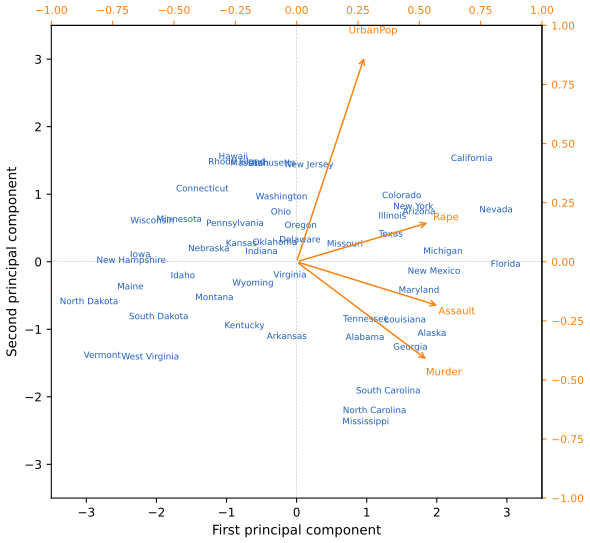
States far to the right (Florida, Nevada, California) have high crime rates on all three counts; North Dakota and Vermont, far left, have low ones; California is also highly urbanised (high PC2), Mississippi and the Carolinas much less so; Indiana, near the origin, is average on both.
12.2.2 Another Interpretation of Principal Components
The loading vectors are the directions of greatest variance; equivalently, they span the lines and planes that are closest to the data. The first loading vector defines the line through the origin with the smallest average squared distance to the \(n\) points; the first two span the closest plane (Figure 12.2), the first three the closest three-dimensional subspace, and so on. Together, the first \(M\) score and loading vectors give the approximation
\[ x_{ij}\approx\sum_{m=1}^Mz_{im}\phi_{jm}, \tag{12.5} \]and this is the best possible approximation of its kind: among all \(\bA\in\R^{n\times M}\), \(\bB\in\R^{p\times M}\), the problem
\[ \min_{\bA,\bB}\ \sum_{j=1}^p\sum_{i=1}^n\Big(x_{ij}-\sum_{m=1}^Ma_{im}b_{jm}\Big)^2 \tag{12.6} \]is solved by \(\hat a_{im}=z_{im}\), \(\hat b_{jm}=\phi_{jm}\), so its smallest value is
\[ \sum_{j=1}^p\sum_{i=1}^n\Big(x_{ij}-\sum_{m=1}^Mz_{im}\phi_{jm}\Big)^2. \tag{12.7} \]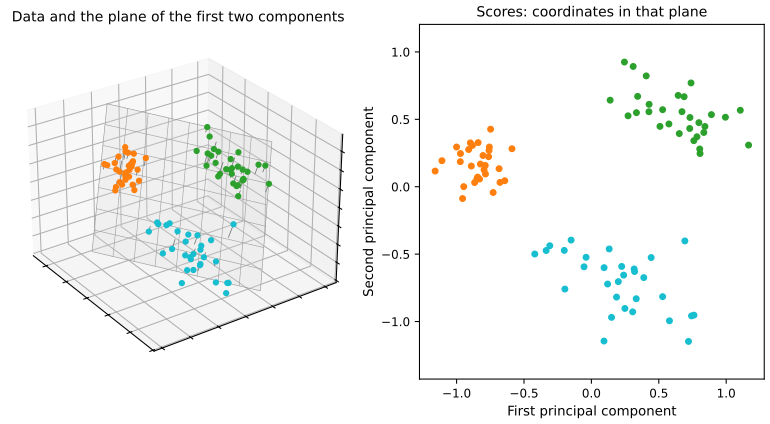
Result 12.2 (principal components give the best low-rank approximation) Section 12.2.2, (12.6)–(12.7) and footnote 4
For every \(M\le r=\rank\bX\), the minimum of (12.6) is \(\sum_{m\gt M}d_m^2=n\sum_{m\gt M}\lambda_m\), attained at \(\bA=\bZ_M=[\bz_1,\dots,\bz_M]\), \(\bB=\bPhi_M=[\bphi_1,\dots,\bphi_M]\), so that \(\bZ_M\bPhi_M^\T=\sum_{m\le M}d_m\bu_m\bv_m^\T\) (the truncated SVD). Every other minimiser has the same product \(\bA\bB^\T\) when \(\lambda_M\gt\lambda_{M+1}\): \(\bA\bB^\T=(\bA\bR)(\bB\bR^{-\T})^\T\) for any invertible \(\bR\), so the factors themselves are not unique. With \(M=r\) the representation is exact.
Filling the gap 12.2: why the first \(M\) components solve (12.6) Section 12.2.2 ("it can be shown")
Derivation
Step 1: reduce to orthonormal \(\bB\). The product \(\bA\bB^\T\) has rank at most \(M\), and conversely every matrix of rank at most \(M\) can be written \(\bA\bB^\T\) with \(\bB\) having \(M\) orthonormal columns that span its row space. So we may assume \(\bB^\T\bB=\bI_M\).
Step 2: the best \(\bA\) for a given \(\bB\). Row \(i\) of the objective is \(\|x_i-\bB a_i\|^2\), a least-squares problem in \(a_i\) with design \(\bB\): its solution is \(a_i=(\bB^\T\bB)^{-1}\bB^\T x_i=\bB^\T x_i\), so \(\bA=\bX\bB\). Then \(\bX\bB\bB^\T\) projects each row on the column space of \(\bB\), and by Pythagoras
\[ \|\bX-\bX\bB\bB^\T\|^2=\|\bX\|^2-\|\bX\bB\bB^\T\|^2=\|\bX\|^2-\|\bX\bB\|^2=\|\bX\|^2-\tr(\bB^\T\bX^\T\bX\bB). \]Step 3: maximise the trace. Write \(\bX^\T\bX=\sum_k\mu_k\be_k\be_k^\T\) with \(\mu_k=n\lambda_k=d_k^2\). Then \(\tr(\bB^\T\bX^\T\bX\bB)=\sum_m\bb_m^\T\bX^\T\bX\bb_m=\sum_k\mu_kh_k\) with \(h_k=\sum_{m=1}^M(\be_k^\T\bb_m)^2\). Each \(h_k\) is the squared length of the projection of the unit vector \(\be_k\) on the column space of \(\bB\), so \(0\le h_k\le1\), and \(\sum_kh_k=\sum_m\|\bb_m\|^2=M\). A sum \(\sum_k\mu_kh_k\) with decreasing weights \(\mu_k\), under these two constraints, is largest when the first \(M\) of the \(h_k\) equal 1 and the rest 0: the maximum is \(\mu_1+\dots+\mu_M\), attained at \(\bB=[\be_1,\dots,\be_M]=\bPhi_M\). (This is Ky Fan's maximum principle.)
Conclusion. The minimum of (12.6) is \(\|\bX\|^2-\sum_{m\le M}d_m^2=\sum_{m\gt M}d_m^2\), with \(\bB=\bPhi_M\) and \(\bA=\bX\bPhi_M=\bZ_M\). If \(\mu_M\gt\mu_{M+1}\), only the column space of \(\bPhi_M\) achieves the maximum, so the product \(\bA\bB^\T\) is unique although the factors are not (footnote 4 of the book). The same result (the Eckart-Young theorem) says that the truncated SVD is the closest rank-\(M\) matrix to \(\bX\); it is the engine of Algorithm 12.1. ∎
12.2.3 The Proportion of Variance Explained
How much is lost by keeping only the first few components? Assuming centred variables, the total variance is
\[ \sum_{j=1}^p\Var(X_j)=\sum_{j=1}^p\frac1n\sum_{i=1}^nx_{ij}^2, \tag{12.8} \]and the variance explained by the \(m\)-th component is
\[ \frac1n\sum_{i=1}^nz_{im}^2=\frac1n\sum_{i=1}^n\Big(\sum_{j=1}^p\phi_{jm}x_{ij}\Big)^2. \tag{12.9} \]Definition 12.2 (proportion of variance explained) Section 12.2.3, (12.10)
The PVE of the \(m\)-th principal component is
\[ \frac{\sum_{i=1}^nz_{im}^2}{\sum_{j=1}^p\sum_{i=1}^nx_{ij}^2}=\frac{\sum_{i=1}^n\big(\sum_{j=1}^p\phi_{jm}x_{ij}\big)^2}{\sum_{j=1}^p\sum_{i=1}^nx_{ij}^2}, \tag{12.10} \]and the cumulative PVE of the first \(M\) components is the sum of their PVEs.
The variance of the data splits into the variance of the first \(M\) components and the mean squared error of the \(M\)-dimensional approximation (12.5):
\[ \underbrace{\sum_{j=1}^p\frac1n\sum_{i=1}^nx_{ij}^2}_{\text{variance of data}}=\underbrace{\sum_{m=1}^M\frac1n\sum_{i=1}^nz_{im}^2}_{\text{variance of first }M\text{ PCs}}+\underbrace{\frac1n\sum_{j=1}^p\sum_{i=1}^n\Big(x_{ij}-\sum_{m=1}^Mz_{im}\phi_{jm}\Big)^2}_{\text{MSE of the approximation}}. \tag{12.11} \]Result 12.3 (the variance decomposition, and why the PVEs sum to one) Section 12.2.3, (12.11)
(a) (12.11) holds for every \(M\). (b) The PVE of component \(m\) is \(\lambda_m/\sum_k\lambda_k=d_m^2/\sum_kd_k^2\). (c) The PVEs of all \(r\) components sum to one, and the cumulative PVE of the first \(M\) is \(1-\RSS/\TSS\), where \(\TSS=\sum_{ij}x_{ij}^2\) and \(\RSS\) is (12.7): it is the \(R^2\) of the rank-\(M\) approximation. (d) So maximising the variance of the first \(M\) components (Section 12.2.1) and minimising the approximation error (Section 12.2.2) are the same problem. For standardised data \(\sum_k\lambda_k=p\) (the trace of the correlation matrix, with the divisor \(n-1\)).
Filling the gap 12.3: proof of (12.11) and of "the PVEs sum to one" Section 12.2.3
Derivation
(a) Pythagoras, row by row. The approximation (12.5) is \(\hat\bX=\bZ_M\bPhi_M^\T=\bX\bPhi_M\bPhi_M^\T\): each row \(x_i\) is replaced by its orthogonal projection on the span of \(\bphi_1,\dots,\bphi_M\). The residual \(x_i-\hat x_i\) is orthogonal to that span, hence to \(\hat x_i\), so \(\|x_i\|^2=\|\hat x_i\|^2+\|x_i-\hat x_i\|^2\). Since \(\bPhi_M\) has orthonormal columns, \(\|\hat x_i\|^2=\|\bPhi_M^\T x_i\|^2=\sum_{m\le M}z_{im}^2\). Summing over \(i\) and dividing by \(n\) gives (12.11).
(b) The PVE as an eigenvalue ratio. By (12.9) and Result 12.1, the variance of \(Z_m\) is \(\lambda_m\). The total variance (12.8) is \(\frac1n\sum_{ij}x_{ij}^2=\tr\bS=\sum_k\lambda_k\), because the trace of a symmetric matrix is the sum of its eigenvalues. So \(\PVE_m=\lambda_m/\sum_k\lambda_k\).
(c) Sum to one. \(\sum_{m=1}^r\PVE_m=\sum_{m\le r}\lambda_m/\sum_k\lambda_k=1\), the eigenvalues beyond \(r\) being zero; equivalently, with \(M=r\) the residual term of (12.11) is zero, since the first \(r\) loading vectors span the row space of \(\bX\). Dividing (12.11) by the total variance gives cumulative PVE \(=1-\RSS/\TSS\).
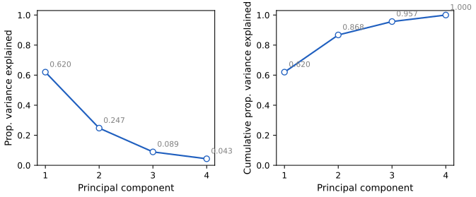
Numbers. For the standardised USArrests data (divisor \(n-1\)) the variances are 2.4802, 0.9898, 0.3566 and 0.1734; they sum to 4 = \(p\), and the PVEs are 0.6201, 0.2474, 0.0891 and 0.0434: 62.0% and 24.7%, together 86.8%, as in the book. ∎
12.2.4 More on PCA
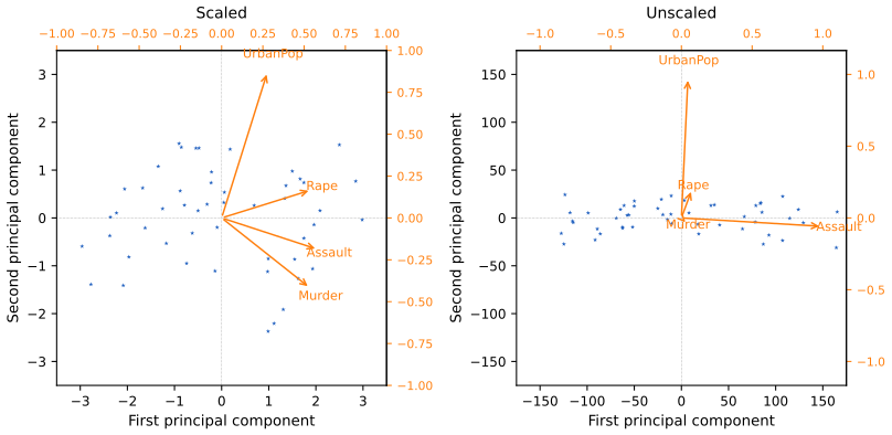
Scaling the variables. Before PCA the variables must be centred; whether they are also scaled (each divided by its standard deviation) changes the answer. In linear regression, rescaling a predictor by \(c\) just rescales its coefficient by \(1/c\); PCA has no such invariance. The USArrests variances are 18.97 (Murder), 87.73 (Rape), 6945.17 (Assault) and 209.52 (UrbanPop), only because of the units (arrests per 100,000 against a percentage). Without scaling, PC1 is almost Assault alone (loading 0.995) and PC2 almost UrbanPop (0.977), as on the right of Figure 12.4. Had Assault been counted per 100 people, its variance would be 0.0069 and it would almost disappear from the first components. To avoid answers that depend on arbitrary units we usually scale; when all variables share the same units (for instance expression levels of genes), one may choose not to.
Result 12.4 (scaling, units and signs) Section 12.2.4
(a) PCA of the standardised variables is the eigen decomposition of the correlation matrix; it is unchanged if any variable is multiplied by a nonzero constant (a change of units), except for the sign of that variable's loadings. PCA of the unscaled variables (the covariance matrix) is not: multiplying \(X_j\) by \(c\) changes the components unless \(X_j\) is uncorrelated with the others. (b) If \(\lambda_m\) is a simple eigenvalue, \(\bphi_m\) is unique up to sign, and flipping it flips \(\bz_m\), leaving every product \(z_{im}\phi_{jm}\) in (12.5) unchanged. If two eigenvalues are equal, the loading vectors are not unique at all: any orthonormal basis of their eigenspace will do.
Filling the gap 12.4: what scaling does to the eigenvectors, and why signs are arbitrary Section 12.2.4
Derivation
(a) Units. Changing units multiplies the columns by constants: \(\bX\mapsto\bX\bD_c\) with \(\bD_c=\diag(c_1,\dots,c_p)\), and the covariance matrix becomes \(\bD_c\bS\bD_c\). Its eigenvectors are in general not those of \(\bS\); for two variables with covariance \(\begin{pmatrix}a&b\\b&c\end{pmatrix}\) the first eigenvector tilts towards the variable with the larger variance, and as \(c_j\to\infty\) it converges to the \(j\)-th coordinate axis (that is Figure 12.4, right). The exception: if \(X_j\) is uncorrelated with the others, \(\be_j\) stays an eigenvector whatever \(c_j\), only its rank among the eigenvalues changes. Standardising replaces \(x_{ij}\) by \(x_{ij}/s_j\), with covariance matrix the correlation matrix \(\bR=\bD_s^{-1}\bS\bD_s^{-1}\), \(\bD_s=\diag(s_j)\). Now \(c_jX_j\) has standard deviation \(|c_j|s_j\), so its standardised version is \(\sign(c_j)\,x_{ij}/s_j\): only the sign can change, and with it the sign of row \(j\) of every loading vector. The correlation matrix, and hence everything in the left panel of Figure 12.4, does not depend on the units.
(b) Signs. If \(\bS\bphi=\lambda\bphi\) then also \(\bS(-\bphi)=\lambda(-\bphi)\), and both have length one: (12.3) cannot tell \(\bphi\) from \(-\bphi\). When \(\lambda_m\) is simple its eigenspace is a line, which contains exactly two unit vectors, \(\pm\bphi_m\). The scores \(\bz_m=\bX\bphi_m\) change sign with \(\bphi_m\), so \(z_{im}\phi_{jm}=(-z_{im})(-\phi_{jm})\). Software picks a sign by an internal convention: prcomp() returns USArrests' PC1 with negative loadings, scikit-learn returns it positive but flips PC2; these notes and the book choose signs so that each loading vector sums to a positive number. If \(\lambda_m=\lambda_{m+1}\), any rotation of \((\bphi_m,\bphi_{m+1})\) within their plane gives equally valid loading vectors, a non-uniqueness that the book does not need because sample eigenvalues are almost never tied. ∎
Uniqueness of the principal components. As Result 12.4(b) shows, two programs can return loading vectors of opposite signs and both be right; the lab meets this when prcomp()'s biplot comes out as the mirror image of Figure 12.1.
Deciding how many principal components to use. An \(n\times p\) matrix has \(\min(n-1,p)\) components, and the aim is to use the smallest number that gives a good understanding of the data. The usual tool is the scree plot (Figure 12.3, left): look for an elbow, a point after which each further component adds little. For USArrests the elbow is after PC2: PC3 explains under 10% and PC4 under 5%. This is admittedly ad hoc, and the question has no objective answer in an unsupervised analysis: look at the first few components, and keep going only while new interesting patterns appear. In a supervised use such as principal components regression, by contrast, the number of components is a tuning parameter chosen by cross-validation (Section 6.3.1).
12.2.5 Other Uses for Principal Components
Regression (principal components regression, Result 6.12), classification and clustering can all be run on the \(n\times M\) matrix of the first \(M\ll p\) score vectors instead of the full \(n\times p\) data. This often gives less noisy results, because the signal in a data set tends to be concentrated in its first few components while the noise is spread over all of them. The lab clusters the NCI60 cell lines on their first five score vectors (Section 12.5.4).
12.3 Missing Values and Matrix Completion
Section 12.3 Suppose 20 of the 200 entries of USArrests had been lost. None of the methods of this book accepts missing values. Dropping the incomplete rows wastes data; replacing \(x_{ij}\) by the mean of the observed values of column \(j\) is common but ignores what the other variables of observation \(i\) say about it. Principal components can exploit the correlation between the variables to impute the missing entries: this is matrix completion. It is appropriate when values are missing at random (a scale's battery was flat), not when the missingness is informative (the patient was too heavy for the scale).
Sometimes the missingness is the point: a matrix of the ratings that \(n\) customers gave to \(p\) films is mostly empty, and filling it in is what a recommender system does. Netflix's early data had \(n=480{,}189\) customers and \(p=17{,}770\) films, with about 99% of the entries missing.
Principal components with missing values. With \(\mathcal O\) the set of observed pairs \((i,j)\), the natural analogue of (12.6) is
\[ \min_{\bA\in\R^{n\times M},\,\bB\in\R^{p\times M}}\ \sum_{(i,j)\in\mathcal O}\Big(x_{ij}-\sum_{m=1}^Ma_{im}b_{jm}\Big)^2. \tag{12.12} \]A solution gives both imputations \(\hat x_{ij}=\sum_m\hat a_{im}\hat b_{jm}\) for \((i,j)\notin\mathcal O\) and (approximately) the principal components. Unlike (12.6), (12.12) has no closed-form solution, but the following algorithm works well.
Algorithm 12.1 (iterative algorithm for matrix completion) Section 12.3, (12.13)–(12.14)
- Create a complete matrix \(\tX\) with \(\tilde x_{ij}=x_{ij}\) if \((i,j)\in\mathcal O\) and \(\tilde x_{ij}=\bar x_j\) (the mean of the observed values of column \(j\)) otherwise.
- Repeat until the objective (12.14) stops decreasing:
- Solve \[ \min_{\bA,\bB}\ \sum_{j=1}^p\sum_{i=1}^n\Big(\tilde x_{ij}-\sum_{m=1}^Ma_{im}b_{jm}\Big)^2 \tag{12.13} \] by computing the principal components of \(\tX\) (its truncated SVD, Result 12.2).
- For each \((i,j)\notin\mathcal O\), set \(\tilde x_{ij}\leftarrow\sum_{m=1}^M\hat a_{im}\hat b_{jm}\).
- Compute the objective \[ \sum_{(i,j)\in\mathcal O}\Big(x_{ij}-\sum_{m=1}^M\hat a_{im}\hat b_{jm}\Big)^2. \tag{12.14} \]
- Return the imputed entries \(\tilde x_{ij}\), \((i,j)\notin\mathcal O\).
This is the "hard impute" algorithm of Mazumder, Hastie and Tibshirani (2010). The book states in a footnote that each iteration decreases (12.14), but that the global minimum of (12.12) is not guaranteed. The first claim has a two-line proof.
Result 12.5 (Algorithm 12.1 never increases its objective) Section 12.3, footnote 6
Let \(F(\bZ)=\sum_{(i,j)\in\mathcal O}(x_{ij}-z_{ij})^2\) for \(n\times p\) matrices \(\bZ\) of rank at most \(M\), and let \(\bZ_t\) be the rank-\(M\) fit \(\hat\bA\hat\bB^\T\) of iteration \(t\). Then \(F(\bZ_t)\le F(\bZ_{t-1})\) for every \(t\), and \(F(\bZ_1)\) is at most the objective of the column-mean fill \(\bZ_0=\bone\bar x^\T\). The objective converges, but possibly to a local minimum of (12.12), and the result depends on the starting values.
Filling the gap 12.5: why each pass lowers (12.14) Section 12.3
Derivation
The filled matrix. After step 2(b) of iteration \(t-1\), the working matrix is \(\tX_t\): observed entries \(x_{ij}\), missing entries copied from \(\bZ_{t-1}\). (At the start \(\bZ_0=\bone\bar x^\T\), the matrix whose every row is the vector of column means; it has rank one, so it is a legitimate rank-\(M\) candidate for every \(M\ge1\).)
A majoriser. Define \(G_t(\bZ)=\|\tX_t-\bZ\|^2\), the objective of (12.13). Split it over observed and missing cells:
\[ G_t(\bZ)=\underbrace{\sum_{(i,j)\in\mathcal O}(x_{ij}-z_{ij})^2}_{F(\bZ)}+\sum_{(i,j)\notin\mathcal O}\big(z_{t-1,ij}-z_{ij}\big)^2\ \ge\ F(\bZ), \]with equality at \(\bZ=\bZ_{t-1}\), where the second sum vanishes: \(G_t(\bZ_{t-1})=F(\bZ_{t-1})\).
The descent. Step 2(a) chooses \(\bZ_t\) to minimise \(G_t\) over rank-\(M\) matrices (Result 12.2), so
\[ F(\bZ_t)\le G_t(\bZ_t)\le G_t(\bZ_{t-1})=F(\bZ_{t-1}). \]The first inequality is the majoriser property, the second the optimality of step 2(a). This is a majorise-minimise (MM) algorithm, the same principle as the EM algorithm. A non-increasing sequence bounded below by 0 converges, so the stopping rule is eventually met. But (12.12) is not convex (the set of rank-\(M\) matrices is not convex), so the limit can be a local minimum.
The labs' stopping rule. Both labs track \(\text{MSS}_t=F(\bZ_t)/|\mathcal O|\) and stop when \((\text{MSS}_{t-1}-\text{MSS}_t)/\text{mss0}\lt10^{-7}\), with mss0 the mean square of the observed entries (dividing by mss0 makes the rule unit-free). The R lab starts \(\text{MSS}_0\) at \(F(\bZ_0)/|\mathcal O|\), the objective of the column-mean fill; the Python lab at mss0 itself, which is \(F(\mathbf 0)/|\mathcal O|\), the objective of the zero matrix. Both are values of \(F\) at rank-\(\le M\) matrices, so the first relative decrease is positive either way, but it differs, and so can the number of iterations. ∎
Illustration on USArrests. On the standardised data, the book hides one randomly chosen variable in each of 20 randomly chosen states (10% of the entries) and runs Algorithm 12.1 with \(M=1\). The 20 entries of Figure 12.5 are exactly those of the R lab (set.seed(15), Section 12.5.2): the algorithm stops after 8 iterations with correlation 0.6535 between imputed and true values.
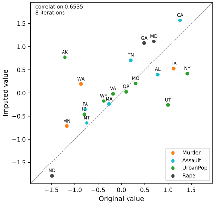
Over 100 random patterns of 20 hidden entries, the book reports an average correlation of \(0.63\pm0.11\) between the true and imputed values, against \(0.79\pm0.08\) for the unattainable "gold standard" that uses the rank-one approximation \(z_{i1}\phi_{j1}\) of the complete data. Our 100 patterns give \(0.641\pm0.115\) and \(0.798\pm0.073\), in agreement. Figure 12.6 shows that the completed matrix also recovers the principal components themselves.
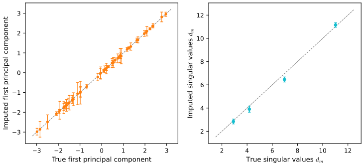
Two remarks from the book. Four variables are few for this method, which is why only one value per state was hidden and \(M=1\) was used (try \(M=2\) in the demonstration: the observed cells are fitted better and the hidden ones much worse). And \(M\) must be chosen: hide a few extra known entries and pick the \(M\) that recovers them best, a validation-set approach (Chapter 5).
Recommender systems. Applied to a ratings matrix, \(\hat x_{ij}=\sum_m\hat a_{im}\hat b_{jm}\) predicts customer \(i\)'s rating of film \(j\). The \(M\) components can be read as "cliques" and "genres": \(\hat a_{im}\) measures how strongly customer \(i\) belongs to clique \(m\), a group of customers who like genre \(m\), and \(\hat b_{jm}\) how strongly film \(j\) belongs to genre \(m\) (romance, western, action, ...). Methods of this kind, made efficient for very sparse matrices (for instance by adding a nuclear-norm penalty, "soft impute"), are at the heart of many recommender systems.
12.4 Clustering Methods
Section 12.4 Clustering partitions the observations into groups such that observations within a group are similar and observations in different groups are not. What "similar" means is a modelling decision, often a scientific one. Examples: unknown subtypes of breast cancer among tissue samples, or market segments among customers. PCA and clustering both simplify the data, but differently: PCA looks for a low-dimensional representation that explains much of the variance, clustering for homogeneous subgroups. The two best-known methods are K-means, for a number \(K\) of clusters fixed in advance, and hierarchical clustering, which builds a tree (a dendrogram) that shows the clusterings for every \(K\) from 1 to \(n\) at once. Observations can be clustered on the basis of the features, or features on the basis of the observations by transposing the data matrix.
12.4.1 K-Means Clustering
Let \(C_1,\dots,C_K\) be the sets of indices of the observations in the \(K\) clusters: they are disjoint and their union is \(\{1,\dots,n\}\). A good clustering has small within-cluster variation \(W(C_k)\):
\[ \min_{C_1,\dots,C_K}\ \Big\{\sum_{k=1}^KW(C_k)\Big\}. \tag{12.15} \]Definition 12.3 (the K-means problem) Section 12.4.1, (12.16)–(12.17)
With squared Euclidean distance, the within-cluster variation of \(C_k\) is the sum of all pairwise squared distances in the cluster, divided by its size:
\[ W(C_k)=\frac1{|C_k|}\sum_{i,i'\in C_k}\sum_{j=1}^p(x_{ij}-x_{i'j})^2, \tag{12.16} \]and K-means clustering is the problem
\[ \min_{C_1,\dots,C_K}\ \Big\{\sum_{k=1}^K\frac1{|C_k|}\sum_{i,i'\in C_k}\sum_{j=1}^p(x_{ij}-x_{i'j})^2\Big\}. \tag{12.17} \]Solving (12.17) exactly is hopeless except for tiny problems: the number of ways to partition \(n\) observations into \(K\) nonempty clusters is the Stirling number of the second kind, about \(K^n/K!\) (the book says "almost \(K^n\)"; see Note 6). For \(n=10\) and \(K=4\) it is already 34,105. A simple algorithm finds a local optimum.
Algorithm 12.2 (K-means clustering) Section 12.4.1
- Randomly assign a number from 1 to \(K\) to each observation: the initial cluster assignments.
- Iterate until the assignments stop changing:
- For each cluster, compute its centroid, the vector of the \(p\) feature means of its observations.
- Assign each observation to the cluster whose centroid is closest in Euclidean distance.
The key to the algorithm is the identity
\[ \frac1{|C_k|}\sum_{i,i'\in C_k}\sum_{j=1}^p(x_{ij}-x_{i'j})^2=2\sum_{i\in C_k}\sum_{j=1}^p(x_{ij}-\bar x_{kj})^2,\qquad\bar x_{kj}=\frac1{|C_k|}\sum_{i\in C_k}x_{ij}. \tag{12.18} \]Result 12.6 (the identity (12.18), and why K-means never increases its objective) Section 12.4.1, Exercise 1
(a) (12.18) holds, so the objective (12.17) is twice the within-cluster sum of squares \(\WSS=\sum_k\sum_{i\in C_k}\|x_i-\bar x_k\|^2\), the quantity R's kmeans() reports as tot.withinss and scikit-learn's KMeans as inertia_. (b) Neither step 2(a) nor step 2(b) of Algorithm 12.2 can increase (12.17), and the algorithm stops after finitely many iterations at a partition where each observation is closest to its own centroid: a local optimum. (c) Different starting assignments can lead to different local optima, so the algorithm should be run from many starts, keeping the best.
Filling the gap 12.6: proof of (12.18) and of the descent property Section 12.4.1
Derivation
(a) The identity. Fix a cluster \(C\) of size \(m\) and a feature \(j\); write \(y_i=x_{ij}-\bar x_{j}\), so that \(\sum_{i\in C}y_i=0\). Since \(x_{ij}-x_{i'j}=y_i-y_{i'}\),
\[ \sum_{i,i'\in C}(y_i-y_{i'})^2=\sum_{i,i'}\big(y_i^2+y_{i'}^2-2y_iy_{i'}\big)=2m\sum_{i\in C}y_i^2-2\Big(\sum_{i\in C}y_i\Big)^2=2m\sum_{i\in C}y_i^2. \]Divide by \(m=|C|\) and sum over \(j\): that is (12.18). (The double sum counts each pair twice and includes \(i=i'\), which contributes zero.)
(b) Descent. For any partition \(C\) and any centres \(\mathbf m_1,\dots,\mathbf m_K\) let \(\Phi(C,\mathbf m)=\sum_k\sum_{i\in C_k}\|x_i-\mathbf m_k\|^2\). For a fixed cluster, \(\sum_{i\in C_k}\|x_i-\mathbf m\|^2=\sum_{i\in C_k}\|x_i-\bar x_k\|^2+|C_k|\,\|\bar x_k-\mathbf m\|^2\) (the cross term vanishes because the deviations from \(\bar x_k\) sum to zero), so the mean is the best centre and \(\WSS(C)=\min_{\mathbf m}\Phi(C,\mathbf m)\). Now one iteration, from partition \(C\) to \(C'\):
- step 2(a) sets \(\mathbf m_k=\bar x_k\), so \(\Phi(C,\mathbf m)=\WSS(C)\);
- step 2(b) gives each observation the centre nearest to it, which cannot increase any term: \(\Phi(C',\mathbf m)\le\Phi(C,\mathbf m)\);
- the next step 2(a) replaces \(\mathbf m\) by the means of \(C'\): \(\WSS(C')\le\Phi(C',\mathbf m)\).
Hence \(\WSS(C')\le\WSS(C)\), and (12.17) \(=2\,\WSS\) never increases. If an observation is reassigned, it moves to a strictly closer centre, so \(\Phi\) and therefore \(\WSS\) strictly decrease; there are finitely many partitions, so no partition can come back and the algorithm stops. At the end no observation would rather be in another cluster: a local optimum, not necessarily the global one.
Counting partitions. The number of ways to split \(n\) labelled observations into \(K\) nonempty unlabelled clusters is the Stirling number \(S(n,K)=\frac1{K!}\sum_{j=0}^K(-1)^j\binom Kj(K-j)^n\). The \(j=0\) term dominates for large \(n\), so \(S(n,K)\approx K^n/K!\): the \(K^n\) labelled assignments, divided by the \(K!\) relabellings of the same partition. ∎
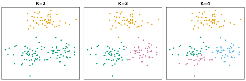
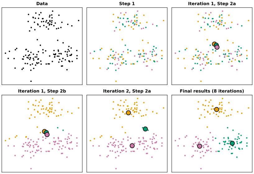
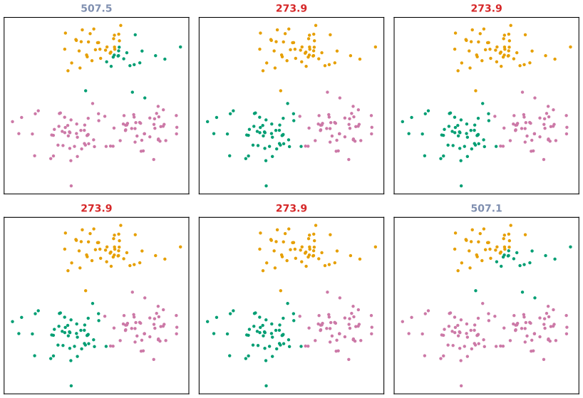
K-means takes its name from step 2(a). In practice: run it from many random starts (R's nstart, scikit-learn's n_init, 20 or 50) and keep the best; set a seed so that the result can be reproduced; and remember that \(K\) must be chosen (Section 12.4.3).
12.4.2 Hierarchical Clustering
Hierarchical clustering does not require \(K\) in advance, and it produces a tree-shaped summary of the data, the dendrogram. We describe the most common, bottom-up or agglomerative, version: the tree is built from the leaves to the trunk.
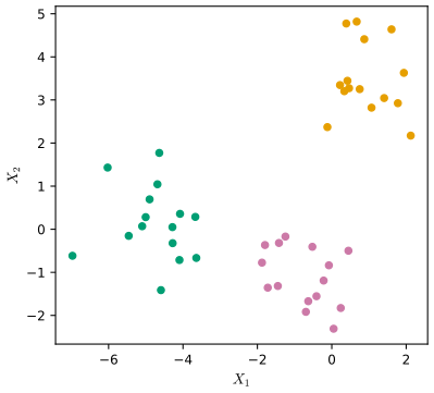
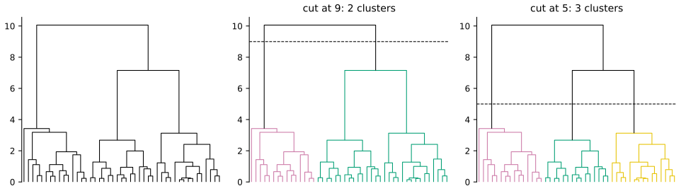
Interpreting a dendrogram. Figure 12.10 shows 45 observations from three classes; Figure 12.11 the dendrogram of complete-linkage clustering. Each leaf is an observation; moving up, leaves fuse into branches and branches into larger branches. The lower two observations fuse, the more similar they are.
Result 12.7 (reading a dendrogram) Section 12.4.2
(a) For any two observations, the height at which the branches containing them first fuse measures how different they are; for complete linkage it is the largest dissimilarity between the two fused groups. (b) The horizontal order of the leaves carries no information: at each of the \(n-1\) fusions the two branches can be swapped, giving \(2^{n-1}\) drawings of the same tree. (c) A horizontal cut at height \(h\) gives one cluster per branch it crosses; cutting at a greater height can only merge clusters.
Filling the gap 12.7: fusion heights and the \(2^{n-1}\) orderings Section 12.4.2
Derivation
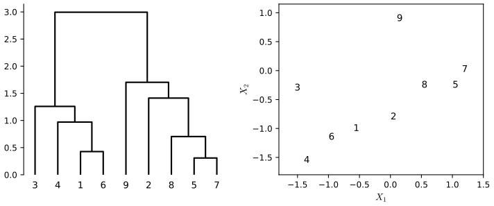
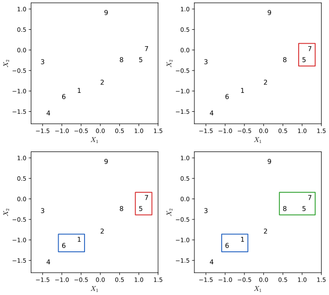
(a) Two observations \(i\) and \(i'\) end up in the same cluster at the fusion of a group \(A\ni i\) with a group \(B\ni i'\); the tree records that fusion at height \(D(A,B)\), the linkage dissimilarity. For complete linkage, \(D(A,B)=\max_{a\in A,b\in B}d(a,b)\ge d(i,i')\), and every pair across \(A\) and \(B\) gets the same height. So in Figure 12.12 observation 9 fuses with the group \(\{2,8,5,7\}\) at one height (1.70 in our version): the tree says that 9 is exactly as similar to 2 as to 8, 5 or 7, although 9 and 2 are drawn side by side.
(b) A dendrogram on \(n\) leaves has \(n-1\) internal nodes (each fusion reduces the number of clusters by one, from \(n\) to 1). Each node has a left and a right branch that can be exchanged without changing which groups fuse at which height; the \(n-1\) exchanges are independent, so there are \(2^{n-1}\) left-to-right orders of the leaves for the same tree (Exercise 2(e)). Proximity along the horizontal axis can therefore not mean similarity.
(c) Cutting at height \(h\) undoes all fusions above \(h\); a higher cut undoes a subset of those, so its clusters are unions of the lower cut's clusters: the clusterings for different \(K\) are nested, which is what "hierarchical" means. (If the fusion heights are monotone, which Result 12.8 guarantees for complete, single and average linkage, cutting into \(K\) clusters is the same as undoing the last \(K-1\) fusions.) ∎
Cutting the tree. A horizontal cut gives the clusters: in Figure 12.11 the height of the cut plays the role of \(K\). One dendrogram gives every number of clusters from 1 (no cut) to \(n\) (cut at height 0), and people often choose one by eye from the fusion heights. But the clusterings at different heights are nested (Result 12.7(c)), and the true groups may not be. The book's example: a group of men and women, evenly split among Americans, Japanese and French people. The best split into two might be by sex and the best split into three by nationality; then no tree can represent both, and hierarchical clustering can do worse than K-means for a given number of clusters (Result 12.9).
The algorithm. Choose a dissimilarity between observations (usually Euclidean distance). Start with each observation in its own cluster; fuse the two most similar clusters; repeat until one cluster remains.
Algorithm 12.3 (hierarchical clustering) Section 12.4.2
- Begin with the \(n\) observations, a dissimilarity measure, and all \(\binom n2=n(n-1)/2\) pairwise dissimilarities. Treat each observation as its own cluster.
- For \(i=n,n-1,\dots,2\):
- Among the \(i\) clusters, find the pair of clusters that are least dissimilar and fuse them. Their dissimilarity is the height of the fusion in the dendrogram.
- Compute the new dissimilarities between the \(i-1\) remaining clusters.
Step 2(b) needs a dissimilarity between groups of observations: the linkage.
| Linkage | Dissimilarity between clusters \(A\) and \(B\) (Table 12.3 of the book, in our words) |
|---|---|
| Complete | The largest of the dissimilarities \(d(a,b)\), \(a\in A\), \(b\in B\) (maximal intercluster dissimilarity). |
| Single | The smallest of them. Single linkage tends to produce long, trailing clusters to which single observations are added one at a time ("chaining"). |
| Average | Their mean, \(\frac1{|A||B|}\sum_{a\in A,b\in B}d(a,b)\). |
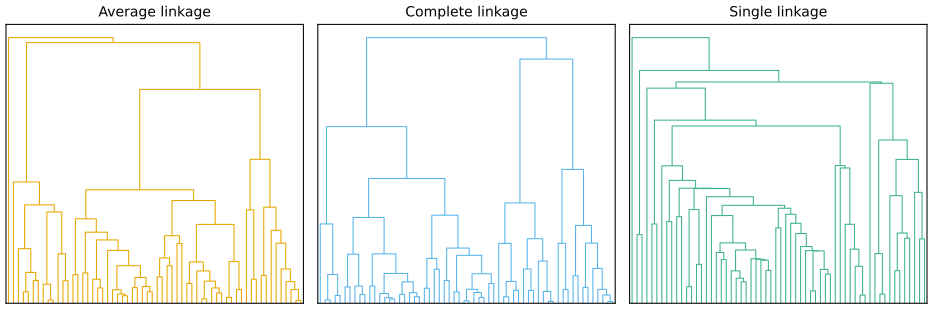
| Centroid | The dissimilarity between the centroids (mean vectors) of \(A\) and \(B\). Popular in genomics, but it can produce inversions: a fusion below an earlier one. |
Average and complete linkage are generally preferred to single linkage because they give more balanced dendrograms (Figure 12.14); the dendrogram depends strongly on the linkage, and on the dissimilarity.
Result 12.8 (no inversions for complete, single and average linkage) Section 12.4.2 and Table 12.3
With complete, single or average linkage the fusion heights of Algorithm 12.3 never decrease, so the dendrogram has no inversions and every horizontal cut is well defined. With centroid linkage an inversion can occur: for three points at the corners of an equilateral triangle with side 1, the first fusion is at height 1 and the second at \(\sqrt3/2\approx0.866\).
Filling the gap 12.8: why the three linkages are monotone, and the inversion Section 12.4.2
Derivation
Monotone heights. Suppose that at some step the closest pair is \((A,B)\) with \(D(A,B)=h\), so every current inter-cluster dissimilarity is at least \(h\). For any other cluster \(C\), the new dissimilarity is
\[ D(A\cup B,C)=\begin{cases}\max\{D(A,C),D(B,C)\}&\text{complete}\\ \min\{D(A,C),D(B,C)\}&\text{single}\\ \frac{|A|D(A,C)+|B|D(B,C)}{|A|+|B|}&\text{average}\end{cases} \](for single and complete linkage the max or min over the pairs of \(A\cup B\) and \(C\) is the max or min of the two groups' values; for average linkage the mean over \(|A\cup B||C|\) pairs is the size-weighted mean of the two means). In all three cases \(D(A\cup B,C)\) lies between \(D(A,C)\) and \(D(B,C)\), both \(\ge h\), so it is \(\ge h\). The dissimilarities between untouched clusters do not change and are \(\ge h\). Hence the next fusion height is \(\ge h\).
The inversion. Centroid linkage has no such "between" property. Put three points at the corners of an equilateral triangle with side 1: all three pairwise distances are 1, so the first fusion, of two corners, is at height 1. Their centroid is the midpoint of that side, whose distance to the third corner is the height of the triangle, \(\sqrt3/2\lt1\). The second fusion happens lower than the first: the branch would have to be drawn hanging below its own children. In the demonstration, centroid linkage produces between 3 and 6 inversions on each of the data sets. ∎
Result 12.9 (cuts of a tree are nested; the best K-means partitions need not be) Section 12.4.2
The clusters obtained by cutting one dendrogram into \(K\) and into \(K-1\) groups are always nested. The partitions minimising (12.17) for \(K-1\) and \(K\) need not be. Example: six equal groups (two sexes in each of three countries), sex shifting the first feature by \(\pm a\) and the countries placed at the corners of an equilateral triangle of side \(s\) in two other features, with little noise. If \(s^2/6\lt a^2\lt s^2/4\), the best two clusters are the sexes and the best three are the countries, while average or complete linkage (which first joins the two sexes of each country, at distance \(2a\lt s\)) gives the countries at \(K=3\) and two countries against one at \(K=2\).
Filling the gap 12.9: the men-and-women example in numbers Section 12.4.2
Derivation
Ignore the noise and let \(N\) be the number of people, \(N/6\) in each cell. The corners of an equilateral triangle of side \(s\) are at distance \(s/\sqrt3\) from its centre, so the squared distance to the centre is \(s^2/3\).
- \(K=2\), by sex: within each sex the countries spread around the triangle's centre: \(\WSS=N s^2/3\).
- \(K=2\), one country against two: the single country spreads only along the sex axis (\(a^2\) each); the other cluster spreads along it too and around the midpoint of a side (\(s^2/4\) each): \(\WSS=\frac N3a^2+\frac{2N}3(a^2+\frac{s^2}4)=N(a^2+\frac{s^2}6)\).
- \(K=3\), by country: \(\WSS=Na^2\).
- \(K=3\), the best partition that refines the split by sex: keep one sex whole and split the other into one country against two: \(\WSS=\frac N2\cdot\frac{s^2}3+\frac N3\cdot\frac{s^2}4=\frac{Ns^2}4\) (the single country contributes nothing).
So the sexes beat the countries at \(K=2\) when \(s^2/3\lt a^2+s^2/6\), that is \(a^2\gt s^2/6\), and the countries win at \(K=3\) when \(a^2\lt s^2/4\). Our simulated data use \(s=1\), \(a=0.46\) (\(a^2=0.21\), between \(1/6\) and \(1/4\)) with 15 people per cell and noise standard deviation 0.07. The best K-means solutions have (12.17) \(=2\,\WSS\) equal to 62.11 (by sex) and 40.65 (by country); complete linkage gives 70.74 at \(K=2\) (one country against two) and 40.65 at \(K=3\). The K-means solution for \(K=3\) is not obtained by splitting either cluster of the solution for \(K=2\): every country is cut in half by sex. ∎
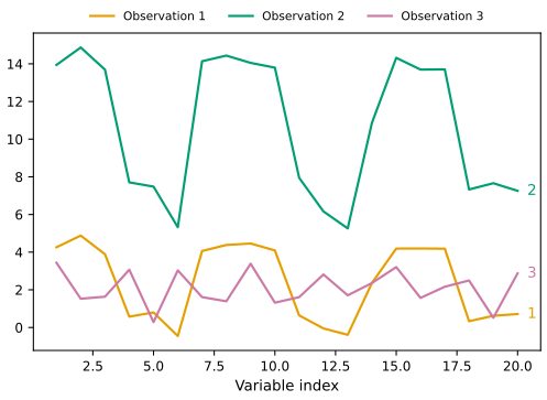
Choice of dissimilarity measure. Euclidean distance is not the only choice. Correlation-based distance treats two observations as similar if their features are highly correlated, even when the values themselves are far apart: it compares the shapes of the profiles, not their levels (Figure 12.15). Here the correlation is computed across the features of two observations, an unusual use of correlation, which is normally computed between variables.
Result 12.10 (correlation-based distance is Euclidean distance between standardised profiles) Section 12.4.2, Exercise 7
If each observation is standardised across its \(p\) features (mean 0, standard deviation 1 with divisor \(p-1\)), then \(\|x_i-x_{i'}\|^2=2(p-1)(1-r_{ii'})\), where \(r_{ii'}\) is the correlation between the two profiles. So clustering with the dissimilarity \(1-r_{ii'}\) is clustering with squared Euclidean distance after standardising each row.
Filling the gap 12.10: one line of algebra Exercise 7
Derivation
After standardising each row, \(\sum_jx_{ij}=0\) and \(\sum_jx_{ij}^2=p-1\), and the correlation of two rows is \(r_{ii'}=\sum_jx_{ij}x_{i'j}/(p-1)\). Then
\[ \|x_i-x_{i'}\|^2=\sum_jx_{ij}^2+\sum_jx_{i'j}^2-2\sum_jx_{ij}x_{i'j}=2(p-1)-2(p-1)r_{ii'}=2(p-1)(1-r_{ii'}). \]With the divisor \(p\) instead, the constant is \(2p\). On USArrests (\(p=4\)), the ratio \(\|x_i-x_{i'}\|^2/(1-r_{ii'})\) equals 6 for all 1,225 pairs of states once each state is standardised; if only the columns are standardised (the usual scaling of variables), the ratio ranges from 0.2 to 11,670, so the two dissimilarities are then quite different (Exercise 7 in the lab). ∎
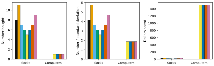
The choice matters and should follow the scientific question. For an online retailer clustering shoppers by purchase counts, Euclidean distance would group together the infrequent shoppers, who bought little of anything; correlation-based distance groups shoppers with similar preferences (items A and B but never C or D), whatever their volume. A related decision is whether to scale the variables first. A shopper buys many pairs of socks and rarely a computer, so raw counts let socks drive the dissimilarities; after scaling each item to standard deviation one, both items count equally; counted in dollars, computers dominate (Figure 12.16). The same question arises for K-means.
12.4.3 Practical Issues in Clustering
Small decisions with big consequences. Should the observations or features be standardised? Which dissimilarity and which linkage? Where to cut the dendrogram, or which \(K\) for K-means? Each choice can change the result strongly. Try several, and look for the solution that is most useful or interpretable: there is no single right answer, and any solution that exposes something interesting deserves attention.
Validating the clusters. Clustering always finds clusters. Whether they are real subgroups or the clustering of noise is hard to tell; methods that attach a \(p\)-value to a cluster exist, but there is no consensus on the best one.
Other considerations. K-means and hierarchical clustering put every observation in some cluster. If a few observations belong to no group, these outliers can distort the clusters badly; mixture models, a "soft" version of K-means, handle them better. Clusterings are also not robust: removing a random subset of the observations and clustering again can give quite different clusters.
A tempered approach. Cluster with several choices of the parameters and look for patterns that persist; cluster subsets of the data to assess robustness; and report clusters as a starting point for hypotheses and further study, ideally on independent data, not as the truth about the data set.
12.5 Lab: Unsupervised Learning
The lab runs PCA and matrix completion on USArrests, K-means and hierarchical clustering on simulated data, and both on the NCI60 cancer cell lines. Every step is shown in R (left; the R lab of James et al. 2021) and Python (right; the Python lab of James et al. 2023), written from scratch for this course: code/ch12_lab.R and code/ch12_lab.py. The Python version uses numpy, pandas, scipy, scikit-learn and matplotlib only; the Python edition's ISLP helpers are replaced by scipy's own linkage(), dendrogram() and cut_tree(). Both files run from start to finish; the outputs below are what they print.
Where R and Python agree, and where they differ
- Identical results wherever the computation is deterministic: the USArrests means and variances, the loading vectors (up to sign), the PVEs, the SVD, the hierarchical clusterings of the same data, and the exercises (the exercises' "random" data are generated by the same formula in both languages, so even Exercises 10 and 11 agree, except K-means with \(K=4\) in Exercise 10). Given the same hidden entries and the same scaling, the matrix-completion iterations agree to every printed digit: the Python file reruns the R lab's entries and prints R's 8 iterations and correlation 0.653504.
- Scaling.
scale()andprcomp(scale = TRUE)divide by the standard deviation with divisor \(n-1\); scikit-learn'sStandardScalerby the one with divisor \(n\). The PVEs are the same, but Python's scores are larger by \(\sqrt{n/(n-1)}\) (standard deviation of the first scores 1.5909 against R's 1.5749 for USArrests), and so are the NCI60 distances and fusion heights (\(\sqrt{64/63}\)): R cuts the NCI60 tree into four clusters at height 139, the Python edition at 140, the same cut. - Random numbers. The two editions simulate different data for the clustering examples and hide different entries in the matrix-completion example (R: correlation 0.6535 after 8 iterations; Python: 0.7114 after 9). R's
kmeans()starts from random centres and uses the Hartigan-Wong algorithm; scikit-learn'sKMeansuses k-means++ starts and Lloyd's algorithm (Algorithm 12.2). On NCI60 with \(K=4\) they stop at different local optima: R's solution has within-cluster sum of squares 344,567 (the R edition's table, up to the numbering of the clusters), Python's 345,903 on R's scale, and the Python edition printed a third partition. The printed inertias of the Python edition (78.06 and 75.04) also depend on the version of scikit-learn; version 1.5 gives 76.85 and 75.06. - Signs.
prcomp()andPCA()choose different signs for the loading vectors (Result 12.4): R's biplot is flipped on PC1, Python's on PC2, and each lab flips back to Figure 12.1.
Setup. Packages (R) and imports (Python). USArrests comes with R; the Python edition downloads it with statsmodels.datasets.get_rdataset(), which needs an internet connection, so the Python file reads a copy exported once from R (as for NCI60, from the R package ISLR2).
R
suppressPackageStartupMessages({
  library(ISLR2)    # NCI60 and Boston (USArrests is in base R)
})
.this_dir <- local({
  a <- grep("^--file=", commandArgs(FALSE), value = TRUE)
  if (length(a)) dirname(normalizePath(sub("^--file=", "", a[1]))) else getwd()
})
img_dir <- file.path(.this_dir, "..", "img", "ch12")
dir.create(img_dir, showWarnings = FALSE, recursive = TRUE)
step <- function(k, title) cat(sprintf("\n== [%s] %s\n", k, title))
options(width = 100, digits = 6)
Python
import os

for _v in ("OPENBLAS_NUM_THREADS", "MKL_NUM_THREADS", "OMP_NUM_THREADS"):
    os.environ.setdefault(_v, "1")

import warnings

import numpy as np
import pandas as pd
from scipy.cluster.hierarchy import linkage, dendrogram, cut_tree
from scipy.stats import norm, ttest_ind
from sklearn.cluster import KMeans, AgglomerativeClustering
from sklearn.decomposition import PCA
from sklearn.preprocessing import StandardScaler

from common import isl_data, savefig, plt, RED, BLUE, ORANGE, GREY
from ch12_unsupervised_learning import usarrests, nci60

warnings.filterwarnings("ignore")
pd.set_option("display.width", 100)
pd.set_option("display.max_columns", 20)
np.set_printoptions(linewidth=100, suppress=True)


def step(k, title):
    print("\n== [%s] %s" % (k, title))
12.5.1 Principal Components Analysis
Step 1: the data. The means differ a lot (on average three times as many rapes as murders and eight times as many assaults as rapes), and so do the variances: without scaling, Assault would drive the components (Result 12.4). Note R's var() and pandas' .var() both divide by \(n-1\).
R
# -- [1] The USArrests data: 50 states, arrests per 100,000 residents and percent urban population
step(1, "The USArrests data")
states <- row.names(USArrests)
head(states, 4)
names(USArrests)
apply(USArrests, 2, mean)
apply(USArrests, 2, var)
Python
# -- [1] The USArrests data: 50 states, arrests per 100,000 residents and percent urban population
step(1, "The USArrests data")
USArrests = usarrests()
print(list(USArrests.index[:4]))
print(list(USArrests.columns))
print(USArrests.mean())
print(USArrests.var())
R output
[1] "Alabama"  "Alaska"   "Arizona"  "Arkansas"
[1] "Murder"   "Assault"  "UrbanPop" "Rape"
  Murder  Assault UrbanPop     Rape
   7.788  170.760   65.540   21.232
   Murder   Assault  UrbanPop      Rape
  18.9705 6945.1657  209.5188   87.7292
Python output
['Alabama', 'Alaska', 'Arizona', 'Arkansas']
['Murder', 'Assault', 'UrbanPop', 'Rape']
Murder        7.788
Assault     170.760
UrbanPop     65.540
Rape         21.232
dtype: float64
Murder        18.970465
Assault     6945.165714
UrbanPop     209.518776
Rape          87.729159
dtype: float64
Step 2: principal components. prcomp(scale = TRUE) centres and scales; its rotation holds the loading vectors as columns and x the scores. In Python, StandardScaler then PCA(): components_ holds the loading vectors as rows. Then the biplot, the standard deviations of the scores, and the PVE (\(\lambda_m/\sum_k\lambda_k\)): 62.0%, 24.7%, 8.9% and 4.3% in both languages.
R
# -- [2] Principal components with prcomp(): centre and scale the columns first
step(2, "Principal components")
pr.out <- prcomp(USArrests, scale = TRUE)
names(pr.out)
pr.out$center
pr.out$scale
pr.out$rotation                       # the loading vectors phi_1, ..., phi_4 (columns)
dim(pr.out$x)                         # the score vectors z_1, ..., z_4 (columns)
pr.out$rotation <- -pr.out$rotation   # flip both signs to get the orientation of Figure 12.1
pr.out$x <- -pr.out$x
pdf(file.path(img_dir, "lab-r-biplot.pdf"), width = 6, height = 6)
biplot(pr.out, scale = 0, cex = 0.6)
invisible(dev.off())
pr.out$sdev
pr.var <- pr.out$sdev^2
pve <- pr.var / sum(pr.var)
pve
pdf(file.path(img_dir, "lab-r-pve.pdf"), width = 8, height = 3.8)
par(mfrow = c(1, 2))
plot(pve, xlab = "Principal Component", ylab = "Proportion of Variance Explained",
     ylim = c(0, 1), type = "b")
plot(cumsum(pve), xlab = "Principal Component", ylab = "Cumulative Proportion of Variance Explained",
     ylim = c(0, 1), type = "b")
invisible(dev.off())
Python
# -- [2] Principal components with scikit-learn: centre and scale the columns first
step(2, "Principal components")
scaler = StandardScaler(with_std=True, with_mean=True)
USArrests_scaled = scaler.fit_transform(USArrests)      # divides by the 1/n standard deviation
pcaUS = PCA()
pcaUS.fit(USArrests_scaled)
print(pcaUS.mean_.round(12))
print(pcaUS.components_)                  # the loading vectors phi_1, ..., phi_4 (rows)
scores = pcaUS.transform(USArrests_scaled)
print(scores.shape)
scores[:, 1] *= -1                        # flip PC2 (scores and loadings) to get Figure 12.1
pcaUS.components_[1] *= -1
fig, ax = plt.subplots(figsize=(6, 6))
ax.scatter(scores[:, 0], scores[:, 1], s=10, color=BLUE)
for k, nm in enumerate(USArrests.columns):
    ax.arrow(0, 0, 2 * pcaUS.components_[0, k], 2 * pcaUS.components_[1, k], color=ORANGE, head_width=0.05)
    ax.text(2.15 * pcaUS.components_[0, k], 2.15 * pcaUS.components_[1, k], nm, color=ORANGE)
ax.set_xlabel("PC1"); ax.set_ylabel("PC2")
savefig(fig, 12, "lab-py-biplot")
print(scores.std(0, ddof=1))
print(pcaUS.explained_variance_)          # the variances of the scores (divisor n - 1)
print(pcaUS.explained_variance_ratio_)    # the PVE (12.10)
fig, axes = plt.subplots(1, 2, figsize=(9, 3.8))
ticks = np.arange(pcaUS.n_components_) + 1
axes[0].plot(ticks, pcaUS.explained_variance_ratio_, marker="o")
axes[0].set_ylabel("Proportion of Variance Explained")
axes[1].plot(ticks, pcaUS.explained_variance_ratio_.cumsum(), marker="o")
axes[1].set_ylabel("Cumulative Proportion of Variance Explained")
for a in axes:
    a.set_xlabel("Principal Component"); a.set_ylim([0, 1]); a.set_xticks(ticks)
savefig(fig, 12, "lab-py-pve")
R output
[1] "sdev"     "rotation" "center"   "scale"    "x"
  Murder  Assault UrbanPop     Rape
   7.788  170.760   65.540   21.232
  Murder  Assault UrbanPop     Rape
 4.35551 83.33766 14.47476  9.36638
               PC1       PC2       PC3        PC4
Murder   -0.535899 -0.418181  0.341233  0.6492278
Assault  -0.583184 -0.187986  0.268148 -0.7434075
UrbanPop -0.278191  0.872806  0.378016  0.1338777
Rape     -0.543432  0.167319 -0.817778  0.0890243
[1] 50  4
[1] 1.574878 0.994869 0.597129 0.416449
[1] 0.6200604 0.2474413 0.0891408 0.0433575
Python output
[-0.  0. -0.  0.]
[[ 0.53589947  0.58318363  0.27819087  0.54343209]
 [-0.41818087 -0.1879856   0.87280619  0.16731864]
 [-0.34123273 -0.26814843 -0.37801579  0.81777791]
 [-0.6492278   0.74340748 -0.13387773 -0.08902432]]
(50, 4)
[1.5908673  1.00496987 0.6031915  0.4206774 ]
[2.53085875 1.00996444 0.36383998 0.17696948]
[0.62006039 0.24744129 0.0891408  0.04335752]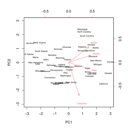
biplot(pr.out, scale = 0) after flipping both signs, the same picture as Figure 12.1. Download: PDF · SVG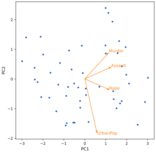
12.5.2 Matrix Completion
Step 3: Algorithm 12.1 written out. First the SVD: the columns of \(\bV\) (R's sX$v; the rows of numpy's third output) are the loading vectors up to sign, and \(\bU\bD\) gives the scores (the printed maximum difference is rounding error). Then 20 entries are hidden, one variable in each of 20 states, and Algorithm 12.1 runs with \(M=1\), each step labelled as in the algorithm. The relative decrease of MSS falls below \(10^{-7}\) after 8 iterations in R and 9 in Python (whose text says eight; Note 4). The Python file then reruns the R lab's entries, scaled as R does: the same 8 iterations and the same correlation, 0.653504. Every MSS is smaller than the one before, as Result 12.5 guarantees.
R
# -- [3] Matrix completion: the SVD, then Algorithm 12.1 by hand
step(3, "Matrix completion")
X <- data.matrix(scale(USArrests))
pcob <- prcomp(X)
summary(pcob)
sX <- svd(X)                           # X = U diag(d) V^T
round(sX$v, 3)                         # = the loadings, up to sign
max(abs(abs(sX$u %*% diag(sX$d)) - abs(pcob$x)))   # U d = the scores, up to sign
nomit <- 20
set.seed(15)
ina <- sample(seq(50), nomit)          # 20 states ...
inb <- sample(1:4, nomit, replace = TRUE)          # ... and one variable in each
ina
inb
Xna <- X
index.na <- cbind(ina, inb)
Xna[index.na] <- NA
fit.svd <- function(X, M = 1) {        # the best rank-M approximation of X
  s <- svd(X)
  s$u[, 1:M, drop = FALSE] %*% (s$d[1:M] * t(s$v[, 1:M, drop = FALSE]))
}
Xhat <- Xna                            # step 1: fill in the column means
xbar <- colMeans(Xna, na.rm = TRUE)
Xhat[index.na] <- xbar[inb]
thresh <- 1e-7
rel_err <- 1
iter <- 0
ismiss <- is.na(Xna)
mssold <- mean((scale(Xna, xbar, FALSE)[!ismiss])^2)
mss0 <- mean(Xna[!ismiss]^2)
while (rel_err > thresh) {
  iter <- iter + 1
  Xapp <- fit.svd(Xhat, M = 1)         # step 2(a)
  Xhat[ismiss] <- Xapp[ismiss]         # step 2(b)
  mss <- mean(((Xna - Xapp)[!ismiss])^2)              # step 2(c): (12.14) / |O|
  rel_err <- (mssold - mss) / mss0
  mssold <- mss
  cat("Iter:", iter, "MSS:", format(mss, digits = 6), "Rel. Err:", format(rel_err, digits = 4), "\n")
}
cor(Xapp[ismiss], X[ismiss])
Python
# -- [3] Matrix completion: the SVD, then Algorithm 12.1 by hand
step(3, "Matrix completion")
X = USArrests_scaled
U, D, V = np.linalg.svd(X, full_matrices=False)   # X = U diag(D) V; the rows of V are the loadings
print(U.shape, D.shape, V.shape)
print(V.round(3))
print(np.abs(np.abs(U * D[None, :]) - np.abs(pcaUS.transform(X))).max())   # U D = the scores, up to sign
n_omit = 20
np.random.seed(15)
r_idx = np.random.choice(np.arange(X.shape[0]), n_omit, replace=False)    # 20 states ...
c_idx = np.random.choice(np.arange(X.shape[1]), n_omit, replace=True)     # ... one variable in each
print(r_idx, c_idx)
Xna = X.copy()
Xna[r_idx, c_idx] = np.nan


def low_rank(X, M=1):
    """The best rank-M approximation of X."""
    U, D, V = np.linalg.svd(X, full_matrices=False)
    return (U[:, :M] * D[None, :M]) @ V[:M]


def complete(Xna, X, M=1, thresh=1e-7, start="py", verbose=True):
    """Algorithm 12.1 with the labs' stopping rule; returns the correlation of imputed and true values."""
    Xhat = Xna.copy()
    Xbar = np.nanmean(Xhat, axis=0)
    ismiss = np.isnan(Xna)
    Xhat[ismiss] = np.broadcast_to(Xbar, Xna.shape)[ismiss]              # step 1: column means
    mss0 = np.mean(Xna[~ismiss] ** 2)
    mssold = mss0 if start == "py" else np.mean((Xna - Xbar)[~ismiss] ** 2)
    rel_err, count = 1.0, 0
    while rel_err > thresh:
        count += 1
        Xapp = low_rank(Xhat, M=M)                                           # step 2(a)
        Xhat[ismiss] = Xapp[ismiss]                                          # step 2(b)
        mss = np.mean(((Xna - Xapp)[~ismiss]) ** 2)                         # step 2(c)
        rel_err = (mssold - mss) / mss0
        mssold = mss
        if verbose:
            print("Iteration: %d, MSS: %.6f, Rel.Err %.3e" % (count, mss, rel_err))
    return np.corrcoef(Xapp[ismiss], X[ismiss])[0, 1]


print(round(complete(Xna, X), 4))
# The R lab removes other entries (R's random numbers) from a matrix scaled with the n - 1 standard
# deviation. With R's entries and R's scaling, the iterations are exactly those of the R lab:
XR = (USArrests - USArrests.mean()) / USArrests.std(ddof=1)
XR = XR.to_numpy()
ina = np.array([37, 47, 42, 34, 38, 5, 25, 12, 20, 46, 1, 43, 50, 23, 2, 44, 10, 26, 21, 32]) - 1
inb = np.array([3, 1, 2, 4, 2, 2, 3, 3, 4, 3, 2, 1, 3, 1, 3, 3, 4, 2, 2, 3]) - 1
XRna = XR.copy()
XRna[ina, inb] = np.nan
print(round(complete(XRna, XR, start="R"), 6))
R output
Importance of components:
                        PC1   PC2    PC3    PC4
Standard deviation     1.57 0.995 0.5971 0.4164
Proportion of Variance 0.62 0.247 0.0891 0.0434
Cumulative Proportion  0.62 0.868 0.9566 1.0000
       [,1]   [,2]   [,3]   [,4]
[1,] -0.536 -0.418  0.341  0.649
[2,] -0.583 -0.188  0.268 -0.743
[3,] -0.278  0.873  0.378  0.134
[4,] -0.543  0.167 -0.818  0.089
[1] 3.33067e-15
 [1] 37 47 42 34 38  5 25 12 20 46  1 43 50 23  2 44 10 26 21 32
 [1] 3 1 2 4 2 2 3 3 4 3 2 1 3 1 3 3 4 2 2 3
Iter: 1 MSS: 0.38217 Rel. Err: 0.6194
Iter: 2 MSS: 0.370505 Rel. Err: 0.01161
Iter: 3 MSS: 0.369278 Rel. Err: 0.001221
Iter: 4 MSS: 0.369123 Rel. Err: 0.0001543
Iter: 5 MSS: 0.369101 Rel. Err: 2.199e-05
Iter: 6 MSS: 0.369097 Rel. Err: 3.376e-06
Iter: 7 MSS: 0.369097 Rel. Err: 5.465e-07
Iter: 8 MSS: 0.369097 Rel. Err: 9.253e-08
[1] 0.653504
Python output
(50, 4) (4,) (4, 4)
[[-0.536 -0.583 -0.278 -0.543]
 [-0.418 -0.188  0.873  0.167]
 [ 0.341  0.268  0.378 -0.818]
 [ 0.649 -0.743  0.134  0.089]]
3.552713678800501e-15
[35 37 41 26 38 43  3 33 30 36 14 16 20  9 44 47 49 22 25 42] [3 3 0 1 0 1 3 1 0 0 3 1 1 0 0 2 2 0 1 2]
Iteration: 1, MSS: 0.395497, Rel.Err 5.986e-01
Iteration: 2, MSS: 0.382364, Rel.Err 1.333e-02
Iteration: 3, MSS: 0.380944, Rel.Err 1.441e-03
Iteration: 4, MSS: 0.380767, Rel.Err 1.794e-04
Iteration: 5, MSS: 0.380742, Rel.Err 2.576e-05
Iteration: 6, MSS: 0.380738, Rel.Err 4.224e-06
Iteration: 7, MSS: 0.380737, Rel.Err 7.649e-07
Iteration: 8, MSS: 0.380737, Rel.Err 1.475e-07
Iteration: 9, MSS: 0.380737, Rel.Err 2.952e-08
0.7114
Iteration: 1, MSS: 0.382170, Rel.Err 6.194e-01
Iteration: 2, MSS: 0.370505, Rel.Err 1.161e-02
Iteration: 3, MSS: 0.369278, Rel.Err 1.221e-03
Iteration: 4, MSS: 0.369123, Rel.Err 1.543e-04
Iteration: 5, MSS: 0.369101, Rel.Err 2.199e-05
Iteration: 6, MSS: 0.369097, Rel.Err 3.376e-06
Iteration: 7, MSS: 0.369097, Rel.Err 5.465e-07
Iteration: 8, MSS: 0.369097, Rel.Err 9.253e-08
0.653504
For real problems the R edition recommends the softImpute package, which adds a penalty on the size of the singular values and scales to very large sparse matrices.
12.5.3 Clustering
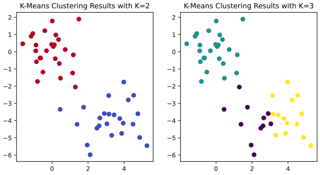
Step 4: K-means. 50 points in two groups (the first 25 shifted by \((3,-4)\)), then K-means with \(K=2\) and \(K=3\). R uses the R edition's seeds and reproduces its numbers exactly: cluster sizes 10, 23 and 17 (printed as 17, 23, 10 in the book, the same partition numbered differently), between-cluster share 79.3%, and tot.withinss 104.33 with one start against 97.98 with 20. The Python data come from numpy's generator, so they differ: there one point of the first group (observation 22, at \((1.29,-2.05)\)) lands in the other cluster with \(K=2\) (Note 5). In both languages the reported criterion is the within-cluster sum of squares, half of (12.17) (Result 12.6).
R
# -- [4] K-means clustering of simulated data with two groups
step(4, "K-means clustering")
set.seed(2)
x <- matrix(rnorm(50 * 2), ncol = 2)
x[1:25, 1] <- x[1:25, 1] + 3
x[1:25, 2] <- x[1:25, 2] - 4
km.out <- kmeans(x, 2, nstart = 20)
km.out$cluster
pdf(file.path(img_dir, "lab-r-kmeans.pdf"), width = 8, height = 4)
par(mfrow = c(1, 2))
plot(x, col = (km.out$cluster + 1), main = "K-Means Clustering Results with K = 2",
     xlab = "", ylab = "", pch = 20, cex = 2)
set.seed(4)
km.out <- kmeans(x, 3, nstart = 20)
plot(x, col = (km.out$cluster + 1), main = "K-Means Clustering Results with K = 3",
     xlab = "", ylab = "", pch = 20, cex = 2)
invisible(dev.off())
km.out$size
km.out$centers
km.out$withinss
km.out$betweenss / km.out$totss
set.seed(4)
km.out <- kmeans(x, 3, nstart = 1)
km.out$tot.withinss
km.out <- kmeans(x, 3, nstart = 20)
km.out$tot.withinss
2 * km.out$tot.withinss                # the objective (12.17) is twice tot.withinss
Python
# -- [4] K-means clustering of simulated data with two groups
step(4, "K-means clustering")
np.random.seed(0)
X = np.random.standard_normal((50, 2))
X[:25, 0] += 3
X[:25, 1] -= 4
kmeans = KMeans(n_clusters=2, random_state=2, n_init=20).fit(X)
print(kmeans.labels_)
fig, axes = plt.subplots(1, 2, figsize=(8, 4))
axes[0].scatter(X[:, 0], X[:, 1], c=kmeans.labels_, cmap="coolwarm")
axes[0].set_title("K-Means Clustering Results with K=2")
kmeans = KMeans(n_clusters=3, random_state=3, n_init=20).fit(X)
axes[1].scatter(X[:, 0], X[:, 1], c=kmeans.labels_, cmap="viridis")
axes[1].set_title("K-Means Clustering Results with K=3")
savefig(fig, 12, "lab-py-kmeans")
print(np.bincount(kmeans.labels_))
kmeans1 = KMeans(n_clusters=3, random_state=3, n_init=1).fit(X)
kmeans20 = KMeans(n_clusters=3, random_state=3, n_init=20).fit(X)
print(round(kmeans1.inertia_, 4), round(kmeans20.inertia_, 4))
print(round(2 * kmeans20.inertia_, 4))      # the objective (12.17) is twice the inertia
R output
 [1] 1 1 1 1 1 1 1 1 1 1 1 1 1 1 1 1 1 1 1 1 1 1 1 1 1 2 2 2 2 2 2 2 2 2 2 2 2 2 2 2 2 2 2 2 2 2 2 2
[49] 2 2
[1] 10 23 17
      [,1]       [,2]
1  2.30015 -2.6962202
2 -0.38204 -0.0874075
3  3.77896 -4.5620080
[1] 19.5614 52.6770 25.7409
[1] 0.793126
[1] 104.332
[1] 97.9793
[1] 195.959
Python output
[0 0 0 0 0 0 0 0 0 0 0 0 0 0 0 0 0 0 0 0 0 1 0 0 0 1 1 1 1 1 1 1 1 1 1 1 1 1 1 1 1 1 1 1 1 1 1 1 1
 1]
[11 25 14]
76.8513 75.0626
150.1252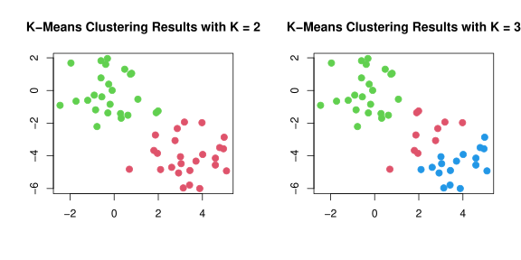
Step 5: hierarchical clustering. Complete, average and single linkage on Euclidean distances; cutree() and cut_tree() cut the trees. With two clusters, complete and average linkage separate the two groups (exactly in R; up to one to three points in Python), while single linkage puts a single observation in a cluster of its own, in both languages. Then the same after scaling the features, and complete linkage with the correlation-based dissimilarity \(1-r\) between observations on 30 points with 3 features (with only two features every correlation between observations would be \(\pm1\)). Python's linkage() takes the dissimilarities in "condensed" form, the upper triangle as a vector; AgglomerativeClustering gives the same clusters as the cut tree.
R
# -- [5] Hierarchical clustering: three linkages, cutting the tree, scaling, correlation distance
step(5, "Hierarchical clustering")
hc.complete <- hclust(dist(x), method = "complete")
hc.average <- hclust(dist(x), method = "average")
hc.single <- hclust(dist(x), method = "single")
pdf(file.path(img_dir, "lab-r-hclust.pdf"), width = 10, height = 4)
par(mfrow = c(1, 3))
plot(hc.complete, main = "Complete Linkage", xlab = "", sub = "", cex = .7)
plot(hc.average, main = "Average Linkage", xlab = "", sub = "", cex = .7)
plot(hc.single, main = "Single Linkage", xlab = "", sub = "", cex = .7)
invisible(dev.off())
cutree(hc.complete, 2)
cutree(hc.average, 2)
cutree(hc.single, 2)
cutree(hc.single, 4)
round(tail(hc.complete$height, 4), 4)  # the last fusion heights
xsc <- scale(x)
table(cutree(hclust(dist(xsc), method = "complete"), 2), cutree(hc.complete, 2))
x <- matrix(rnorm(30 * 3), ncol = 3)   # 30 observations, 3 features, no true clusters
dd <- as.dist(1 - cor(t(x)))           # correlation between observations, not variables
hc.cor <- hclust(dd, method = "complete")
round(tail(hc.cor$height, 3), 4)
Python
# -- [5] Hierarchical clustering: three linkages, cutting the tree, scaling, correlation distance
step(5, "Hierarchical clustering")
linkage_comp = linkage(X, method="complete")      # Euclidean distances by default
linkage_avg = linkage(X, method="average")
linkage_sing = linkage(X, method="single")
cargs = {"color_threshold": -np.inf, "above_threshold_color": "black"}
fig, axes = plt.subplots(1, 3, figsize=(12, 4))
for ax, L, t in zip(axes, (linkage_comp, linkage_avg, linkage_sing), ("Complete", "Average", "Single")):
    dendrogram(L, ax=ax, leaf_font_size=6, **cargs)
    ax.set_title(t + " Linkage")
savefig(fig, 12, "lab-py-hclust")
print(cut_tree(linkage_comp, n_clusters=4).T)
print(cut_tree(linkage_comp, height=5).T)
for L in (linkage_comp, linkage_avg, linkage_sing):
    print(cut_tree(L, n_clusters=2).ravel())
print(linkage_comp[-4:, 2].round(4))           # the last fusion heights
hc = AgglomerativeClustering(n_clusters=4, linkage="complete").fit(X)
print(pd.crosstab(hc.labels_, cut_tree(linkage_comp, n_clusters=4).ravel()))
X_scale = StandardScaler().fit_transform(X)
print(pd.crosstab(cut_tree(linkage(X_scale, "complete"), 2).ravel(), cut_tree(linkage_comp, 2).ravel()))
X3 = np.random.standard_normal((30, 3))        # 30 observations, 3 features, no true clusters
corD = 1 - np.corrcoef(X3)                     # correlation between observations (rows)
iu = np.triu_indices(30, 1)
linkage_cor = linkage(corD[iu], method="complete")   # linkage() takes the condensed distances
print(linkage_cor[-3:, 2].round(4))
R output
 [1] 1 1 1 1 1 1 1 1 1 1 1 1 1 1 1 1 1 1 1 1 1 1 1 1 1 2 2 2 2 2 2 2 2 2 2 2 2 2 2 2 2 2 2 2 2 2 2 2
[49] 2 2
 [1] 1 1 1 1 1 1 1 1 1 1 1 1 1 1 1 1 1 1 1 1 1 1 1 1 1 2 2 2 2 2 2 2 1 2 2 2 2 2 2 2 2 2 2 1 2 1 2 2
[49] 2 2
 [1] 1 1 1 1 1 1 1 1 1 1 1 1 1 1 1 2 1 1 1 1 1 1 1 1 1 1 1 1 1 1 1 1 1 1 1 1 1 1 1 1 1 1 1 1 1 1 1 1
[49] 1 1
 [1] 1 1 1 1 1 1 1 1 1 1 1 1 1 1 1 2 1 1 1 1 1 1 1 1 1 3 3 3 3 3 3 3 3 3 3 3 3 3 3 3 3 4 3 3 3 3 3 3
[49] 3 3
[1] 3.8417 4.7213 4.9206 9.6589

     1  2
  1 25  0
  2  0 25
[1] 1.6526 1.9952 1.9998
Python output
[[0 1 0 0 1 1 0 1 0 0 2 0 0 0 1 1 0 0 1 0 0 2 0 2 2 3 2 3 3 3 3 2 3 3 3 3 2 3 3 3 3 2 3 3 3 3 3 3
  3 3]]
[[0 0 0 0 0 0 0 0 0 0 1 0 0 0 0 0 0 0 0 0 0 1 0 1 1 2 1 2 2 2 2 1 2 2 2 2 1 2 2 2 2 1 2 2 2 2 2 2
  2 2]]
[0 0 0 0 0 0 0 0 0 0 1 0 0 0 0 0 0 0 0 0 0 1 0 1 1 1 1 1 1 1 1 1 1 1 1 1 1 1 1 1 1 1 1 1 1 1 1 1 1
 1]
[0 0 0 0 0 0 0 0 0 0 0 0 0 0 0 0 0 0 0 0 0 1 0 0 0 1 1 1 1 1 1 1 1 1 1 1 1 1 1 1 1 1 1 1 1 1 1 1 1
 1]
[0 0 0 0 0 0 0 0 0 0 0 0 0 0 0 0 0 0 0 0 0 0 0 0 0 0 0 0 0 0 0 0 0 0 0 0 0 0 0 0 0 0 1 0 0 0 0 0 0
 0]
[3.5766 4.6159 6.1543 9.0897]
col_0   0  1  2   3
row_0
0       0  0  8   0
1      14  0  0   0
2       0  0  0  21
3       0  7  0   0
col_0   0   1
row_0
0      21   0
1       0  29
[1.4183 1.9804 2.    ]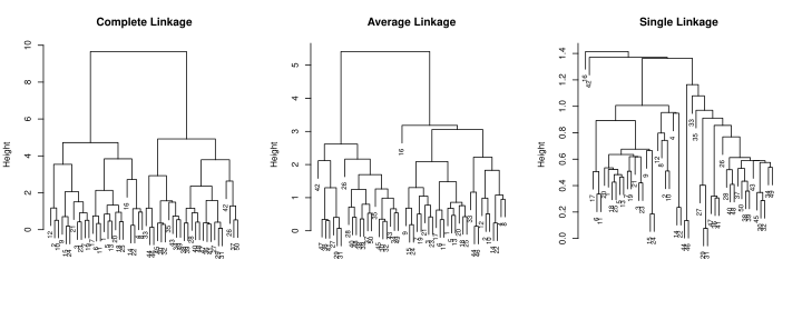
plot(hclust(...)) for complete, average and single linkage. Download: PDF · SVG12.5.4 NCI60 Data Example
Step 6: PCA of the NCI60 data. 64 cancer cell lines, 6,830 gene expression measurements each, with cancer types used only to colour the plots afterwards. PCA on the scaled genes (one could argue for not scaling: all genes are measured in the same units). R's and Python's scores have opposite signs on PC1 and PC2 and differ by the factor \(\sqrt{64/63}=1.0079\) (19.6824 against 19.8380); the PVEs agree: 11.4% for PC1, 38.5% for the first seven together, 100% at the 63rd component.
R
# -- [6] The NCI60 data: principal components of 64 cell lines x 6830 genes
step(6, "NCI60: principal components")
nci.labs <- NCI60$labs
nci.data <- NCI60$data
dim(nci.data)
nci.labs[1:4]
table(nci.labs)
pr.out <- prcomp(nci.data, scale = TRUE)
round(pr.out$x[1:3, 1:3], 4)
Cols <- function(vec) {
  cols <- rainbow(length(unique(vec)))
  cols[as.numeric(as.factor(vec))]
}
pdf(file.path(img_dir, "lab-r-nci-pcs.pdf"), width = 8, height = 4)
par(mfrow = c(1, 2))
plot(pr.out$x[, 1:2], col = Cols(nci.labs), pch = 19, xlab = "Z1", ylab = "Z2")
plot(pr.out$x[, c(1, 3)], col = Cols(nci.labs), pch = 19, xlab = "Z1", ylab = "Z3")
invisible(dev.off())
summary(pr.out)$importance[, 1:6]
pve <- 100 * pr.out$sdev^2 / sum(pr.out$sdev^2)
round(cumsum(pve)[c(5, 7, 10, 20, 63, 64)], 4)
Python
# -- [6] The NCI60 data: principal components of 64 cell lines x 6830 genes
step(6, "NCI60: principal components")
nci_data, nci_labs = nci60()
nci_labs = pd.Series(nci_labs, name="label")
print(nci_data.shape)
print(list(nci_labs[:4]))
print(nci_labs.value_counts().to_dict())
nci_scaled = StandardScaler().fit_transform(nci_data)
nci_pca = PCA()
nci_scores = nci_pca.fit_transform(nci_scaled)
print(nci_scores[:3, :3].round(4))
fig, axes = plt.subplots(1, 2, figsize=(10, 4.2))
cancer_types = sorted(nci_labs.unique())
groups = np.array([cancer_types.index(l) for l in nci_labs])
for ax, j in zip(axes, (1, 2)):
    ax.scatter(nci_scores[:, 0], nci_scores[:, j], c=groups, cmap="tab20", s=30)
    ax.set_xlabel("PC1"); ax.set_ylabel("PC%d" % (j + 1))
savefig(fig, 12, "lab-py-nci-pcs")
print(nci_pca.explained_variance_ratio_[:6].round(5))
print((100 * nci_pca.explained_variance_ratio_.cumsum()[[4, 6, 9, 19, 62, 63]]).round(4))
R output
[1]   64 6830
[1] "CNS"   "CNS"   "CNS"   "RENAL"
nci.labs
     BREAST         CNS       COLON K562A-repro K562B-repro    LEUKEMIA MCF7A-repro MCF7D-repro
          7           5           7           1           1           6           1           1
   MELANOMA       NSCLC     OVARIAN    PROSTATE       RENAL     UNKNOWN
          8           9           6           2           9           1
        PC1    PC2      PC3
V1 -19.6824 3.5277  -9.7354
V2 -22.9081 6.3909 -13.3725
V3 -27.2408 2.4458  -3.5053
                            PC1      PC2      PC3      PC4      PC5      PC6
Standard deviation     27.85347 21.48136 19.82046 17.03256 15.97181 15.72108
Proportion of Variance  0.11359  0.06756  0.05752  0.04248  0.03735  0.03619
Cumulative Proportion   0.11359  0.18115  0.23867  0.28115  0.31850  0.35468
[1]  31.8495  38.5344  46.1256  64.7892 100.0000 100.0000
Python output
(64, 6830)
['CNS', 'CNS', 'CNS', 'RENAL']
{'RENAL': 9, 'NSCLC': 9, 'MELANOMA': 8, 'BREAST': 7, 'COLON': 7, 'OVARIAN': 6, 'LEUKEMIA': 6, 'CNS': 5, 'PROSTATE': 2, 'UNKNOWN': 1, 'K562B-repro': 1, 'K562A-repro': 1, 'MCF7A-repro': 1, 'MCF7D-repro': 1}
[[ 19.838   -3.5556  -9.8124]
 [ 23.0892  -6.4415 -13.4783]
 [ 27.4561  -2.4651  -3.5331]]
[0.11359 0.06756 0.05752 0.04248 0.03735 0.03619]
[ 31.8495  38.5344  46.1256  64.7892 100.     100.    ]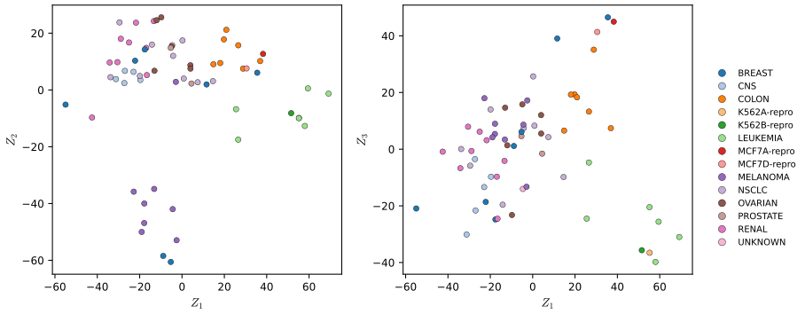
prcomp() as in the book. Cell lines of the same cancer type tend to lie close together, which could not have been seen in any of the \(\binom{6830}2\) scatter plots of pairs of genes. Reproduces James et al. (2021), Figure 12.17. Download: PDF · SVG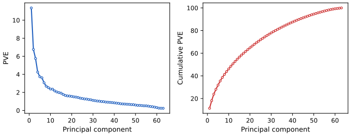
Step 7: clustering the cell lines. Hierarchical clustering of the scaled data with complete, average and single linkage (Figure 12.19), then the complete-linkage tree cut into four clusters. All leukemia lines fall in one cluster (with the two K562 lines), while the breast cancer lines are spread over three. Four clusters result from any cut between the fusion heights 137.56 and 141.25, so the R lab's line at 139 is a valid cut. K-means with \(K=4\) on the same data disagrees with the cut tree: R's solution reproduces the leukemia cluster exactly and splits the large cluster of 40 lines in three, scikit-learn's adds one more line to the leukemia cluster, and (Section 12.2.5) clustering on the first five score vectors gives yet another, but related, partition.
R
# -- [7] Clustering the NCI60 cell lines
step(7, "NCI60: clustering")
sd.data <- scale(nci.data)
data.dist <- dist(sd.data)
pdf(file.path(img_dir, "lab-r-nci-hclust.pdf"), width = 10, height = 12)
par(mfrow = c(3, 1))
plot(hclust(data.dist), xlab = "", sub = "", ylab = "", labels = nci.labs, main = "Complete Linkage",
     cex = 0.6)
plot(hclust(data.dist, method = "average"), labels = nci.labs, main = "Average Linkage",
     xlab = "", sub = "", ylab = "", cex = 0.6)
plot(hclust(data.dist, method = "single"), labels = nci.labs, main = "Single Linkage",
     xlab = "", sub = "", ylab = "", cex = 0.6)
invisible(dev.off())
hc.out <- hclust(dist(sd.data))
hc.clusters <- cutree(hc.out, 4)
table(hc.clusters, nci.labs)[, c("BREAST", "CNS", "COLON", "LEUKEMIA", "MELANOMA", "NSCLC",
                                 "OVARIAN", "RENAL")]
round(tail(hc.out$height, 4), 2)       # four clusters for any cut between 137.56 and 141.25
pdf(file.path(img_dir, "lab-r-nci-cut.pdf"), width = 10, height = 5)
plot(hc.out, labels = nci.labs, cex = 0.55, xlab = "", sub = "")
abline(h = 139, col = "red")
invisible(dev.off())
hc.out
set.seed(2)
km.out <- kmeans(sd.data, 4, nstart = 20)
km.clusters <- km.out$cluster
table(km.clusters, hc.clusters)
km.out$tot.withinss
hc.pc <- hclust(dist(pr.out$x[, 1:5]))
table(cutree(hc.pc, 4), nci.labs)[, c("BREAST", "CNS", "COLON", "LEUKEMIA", "MELANOMA", "NSCLC",
                                      "OVARIAN", "RENAL")]
Python
# -- [7] Clustering the NCI60 cell lines
step(7, "NCI60: clustering")
trees = {m: linkage(nci_scaled, method=m) for m in ("complete", "average", "single")}
comp_cut = cut_tree(trees["complete"], n_clusters=4).ravel()
show = ["BREAST", "CNS", "COLON", "LEUKEMIA", "MELANOMA", "NSCLC", "OVARIAN", "RENAL"]
print(pd.crosstab(pd.Series(comp_cut, name="Complete"), nci_labs)[show])
print(trees["complete"][-4:, 2].round(2))      # the data are scaled with 1/n: heights x sqrt(64/63)
fig, ax = plt.subplots(figsize=(11, 5))
dendrogram(trees["complete"], ax=ax, labels=np.asarray(nci_labs), leaf_font_size=6,
           color_threshold=140, above_threshold_color="black")
ax.axhline(140, c="r", linewidth=2)
savefig(fig, 12, "lab-py-nci-cut")
nci_kmeans = KMeans(n_clusters=4, random_state=0, n_init=20).fit(nci_scaled)
print(pd.crosstab(pd.Series(comp_cut, name="HClust"), pd.Series(nci_kmeans.labels_, name="K-means")))
print(round(nci_kmeans.inertia_ * 63 / 64, 1))  # on R's scale, to compare with R's tot.withinss
hc_pca = linkage(nci_scores[:, :5], method="complete")
print(pd.crosstab(pd.Series(cut_tree(hc_pca, n_clusters=4).ravel(), name="Complete-PCA"), nci_labs)[show])
R output
           nci.labs
hc.clusters BREAST CNS COLON LEUKEMIA MELANOMA NSCLC OVARIAN RENAL
          1      2   3     2        0        8     8       6     8
          2      3   2     0        0        0     1       0     1
          3      0   0     0        6        0     0       0     0
          4      2   0     5        0        0     0       0     0
[1] 137.56 141.25 142.92 162.21

Call:
hclust(d = dist(sd.data))

Cluster method   : complete
Distance         : euclidean
Number of objects: 64

           hc.clusters
km.clusters  1  2  3  4
          1  0  0  8  0
          2 11  0  0  9
          3 20  7  0  0
          4  9  0  0  0
[1] 344567
   nci.labs
    BREAST CNS COLON LEUKEMIA MELANOMA NSCLC OVARIAN RENAL
  1      0   2     7        2        1     8       5     7
  2      5   3     0        0        7     1       1     2
  3      0   0     0        4        0     0       0     0
  4      2   0     0        0        0     0       0     0
Python output
label     BREAST  CNS  COLON  LEUKEMIA  MELANOMA  NSCLC  OVARIAN  RENAL
Complete
0              2    3      2         0         8      8        6      8
1              3    2      0         0         0      1        0      1
2              0    0      0         6         0      0        0      0
3              2    0      5         0         0      0        0      0
[138.65 142.36 144.05 163.49]
K-means  0   1   2  3
HClust
0        1  20  10  9
1        0   7   0  0
2        8   0   0  0
3        0   0   9  0
345902.9
label         BREAST  CNS  COLON  LEUKEMIA  MELANOMA  NSCLC  OVARIAN  RENAL
Complete-PCA
0                  0    2      7         2         1      8        5      7
1                  5    3      0         0         7      1        1      2
2                  0    0      0         4         0      0        0      0
3                  2    0      0         0         0      0        0      0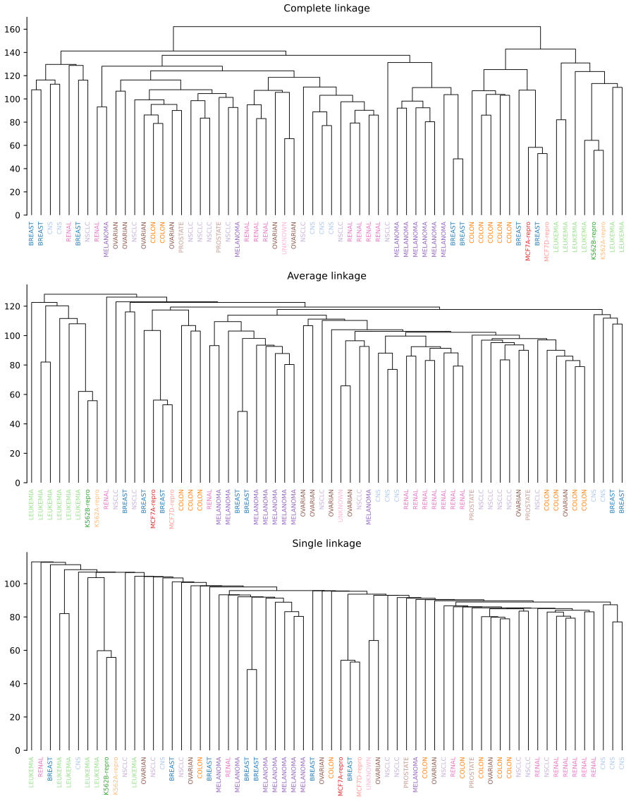
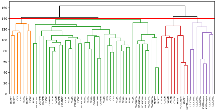
Notes on the book
Points where the text, a figure or a lab of either edition does not match what the computations give, each with the evidence. None changes the methods.
Note 1. Figure 12.6, right panel: singular values, not variances or loadings
The axes of the right panel read "True PC Variances" and "Imputed PC Variances", and the caption says that it shows the imputed principal component loadings against the true loadings. The four plotted values, about 11, 7, 4.2 and 2.9 on the true axis, are neither: loadings lie in \([-1,1]\), and the variances of the components of the standardised data are 2.48, 0.99, 0.36 and 0.17. They are the singular values of the standardised data matrix, \(d_m=\sqrt{(n-1)\lambda_m}\): 11.02, 6.96, 4.18 and 2.92. Our Figure 12.6 plots and labels them as such.
Note 2. "The 50 × 2 data matrix" (R edition, Section 12.5.2)
The R lab says "We now omit 20 entries in the 50 × 2 data matrix at random". The USArrests matrix is \(50\times4\), and the code picks a column from 1:4; the Python edition has "50 × 4".
Note 3. Exercise 6 (R edition): \(p\) regressions, not \(M\)
The R edition asks to show that the loading vectors can be obtained "by performing \(M\) separate least squares linear regressions", one feature of the data matrix being the response in each. There is one regression per feature, so \(p\) of them (each with the \(M\) score vectors as predictors): see the solution of Exercise 6. The Python edition says \(p\).
Note 4. "After eight iterations" (Python edition, Section 12.5.2)
The Python lab prints nine iterations (the eighth has relative error \(1.48\times10^{-7}\), still above the threshold \(10^{-7}\); the ninth \(2.95\times10^{-8}\)) and then says "after eight iterations, the relative error has fallen below thresh". The sentence was carried over from the R edition, where the run stops after eight. Our Python lab reproduces the nine iterations digit for digit.
Note 5. "Perfectly separated" (Python edition, Section 12.5.3)
After KMeans(n_clusters=2, ...) the Python lab states that K-means "perfectly separated the observations into two clusters", but the labels it prints just above give the 22nd observation (index 21) the label of the second group. That point, \((1.29,-2.05)\), was drawn from the shifted group but lies nearer the other group's centroid; with any \(K=2\) clustering of these data it goes to the other cluster. The R edition's data (another random sample) are perfectly separated, and the sentence comes from there.
Note 6. The number of partitions, and "decrease" (Section 12.4.1)
The text says there are "almost \(K^n\) ways to partition \(n\) observations into \(K\) clusters". The number of partitions into \(K\) nonempty clusters is the Stirling number \(S(n,K)\approx K^n/K!\) (Filling the gap 12.6): \(K^n\) counts labelled assignments, each partition being counted \(K!\) times. For \(n=10\), \(K=4\): 34,105 partitions against \(4^{10}=1{,}048{,}576\). The conclusion (far too many to search) stands. The same paragraph says that Algorithm 12.2 "is guaranteed to decrease the value of the objective at each step"; it cannot increase it, and decreases it strictly only while observations change cluster, as the next sentences of the book say.
Note 7. tot.withinss and inertia_ are half of (12.17)
Both labs describe km.out$tot.withinss (R) and kmeans.inertia_ (Python) as "the total within-cluster sum of squares, which we seek to minimize by performing K-means clustering (12.17)". By (12.18) the objective (12.17) is twice that sum (Result 12.6): 195.96 rather than 97.98 for the R lab's best \(K=3\) solution. The two have the same minimisers, so nothing else changes; but the objective values printed above the panels of Figure 12.9 (235.8, 310.9, 320.9) cannot be checked, since the simulated data are not published.
Note 8. Eigenvalues of \(\bX^\T\bX\) are not the variances (footnote 2), and a typo
Footnote 2 of Section 12.2.1 says that the loading vectors are the eigenvectors of \(\bX^\T\bX\) "and the variances of the components are the eigenvalues". The eigenvectors are right, but the eigenvalues of \(\bX^\T\bX\) are \(d_m^2\), which is \(n\) times the variances (12.9), or \(n-1\) times those that prcomp() reports (Result 12.1(c)); the variances are the eigenvalues of \(\bX^\T\bX/n\). Also, the R edition writes "UrpanPop" for UrbanPop below Figure 12.4.
12.6 Exercises
Conceptual exercises 1–6 and applied exercises 7–13, in the book's numbering (the two editions have the same exercises, with the R and Python function names swapped). The applied solutions, and the computations for Exercises 2 and 3, are the last sections of ch12_lab.R and ch12_lab.py. Where an exercise asks for random data, both files use the same deterministic formula in place of a random number generator, so that the two languages give the same numbers:
R
# A deterministic stand-in for random numbers, so that R and Python use the same "random" data:
# u = fractional part of |sin(12.9898 i + 78.233 j + 37.719 s)| x 43758.5453.
hash_u <- function(i, j, s = 0) {
  v <- abs(sin(12.9898 * i + 78.233 * j + 37.719 * s)) * 43758.5453
  pmin(pmax(v - floor(v), 1e-12), 1 - 1e-12)
}
Python
def hash_u(i, j, s=0):
    """A deterministic stand-in for random numbers, identical in R and Python (see ch12_lab.R)."""
    v = np.abs(np.sin(12.9898 * np.asarray(i, float) + 78.233 * np.asarray(j, float) + 37.719 * s)) * 43758.5453
    return np.clip(v - np.floor(v), 1e-12, 1 - 1e-12)
Exercise 12.1. (a) Prove the identity (12.18). (b) Use it to argue that every iteration of Algorithm 12.2 decreases (more precisely, does not increase) the objective (12.17).
Solution
(a) For one cluster and one feature, with \(y_i=x_{ij}-\bar x_{kj}\) summing to zero over the cluster, \(\sum_{i,i'}(y_i-y_{i'})^2=2|C_k|\sum_iy_i^2-2(\sum_iy_i)^2=2|C_k|\sum_iy_i^2\); divide by \(|C_k|\) and sum over \(j\). (b) By (a), (12.17) is \(2\sum_k\sum_{i\in C_k}\|x_i-\bar x_k\|^2\). Step 2(a) puts each centre at its cluster mean, the point that minimises the sum of squared distances to the cluster's observations; step 2(b) moves each observation to the nearest centre, which cannot increase its squared distance; recomputing the means can only lower the sum further. The full argument, with termination, is Filling the gap 12.6.
Exercise 12.2. Four observations have the dissimilarities \(d_{12}=0.3\), \(d_{13}=0.4\), \(d_{14}=0.7\), \(d_{23}=0.5\), \(d_{24}=0.8\), \(d_{34}=0.45\). (a) Sketch the complete-linkage dendrogram, with fusion heights. (b) The same with single linkage. (c), (d) Cut each into two clusters. (e) Draw a dendrogram equivalent to (a) with the leaves rearranged.
Solution
(a) Complete linkage: \(\{1\},\{2\}\) fuse at 0.3 (the smallest dissimilarity). New dissimilarities: \(D(\{1,2\},3)=\max(0.4,0.5)=0.5\), \(D(\{1,2\},4)=\max(0.7,0.8)=0.8\); with \(d_{34}=0.45\) the smallest, \(\{3\},\{4\}\) fuse at 0.45. Finally \(D(\{1,2\},\{3,4\})=\max(0.4,0.5,0.7,0.8)=0.8\). (b) Single linkage: \(\{1,2\}\) at 0.3; then \(D(\{1,2\},3)=\min(0.4,0.5)=0.4\lt0.45\), so 3 joins at 0.4; then 4 joins at \(\min(0.7,0.8,0.45)=0.45\). (c) Complete: \(\{1,2\}\) and \(\{3,4\}\). (d) Single: \(\{1,2,3\}\) and \(\{4\}\). (e) Swapping the two branches at every fusion gives the leaf order 4, 3, 2, 1 with the same fusions at the same heights (right panel below); any of the \(2^3=8\) orders obtained by swaps is equivalent.
R
# -- [E2] Exercise 2: complete and single linkage from a dissimilarity matrix
step("E2", "Exercise 2")
D2 <- as.dist(matrix(c(0, 0.3, 0.4, 0.7, 0.3, 0, 0.5, 0.8, 0.4, 0.5, 0, 0.45, 0.7, 0.8, 0.45, 0), 4))
hc2c <- hclust(D2, method = "complete")
hc2s <- hclust(D2, method = "single")
hc2c$merge; hc2c$height
hc2s$merge; hc2s$height
cutree(hc2c, 2)
cutree(hc2s, 2)
Python
# -- [E2] Exercise 2: complete and single linkage from a dissimilarity matrix
step("E2", "Exercise 2")
D2 = np.array([[0, 0.3, 0.4, 0.7], [0.3, 0, 0.5, 0.8], [0.4, 0.5, 0, 0.45], [0.7, 0.8, 0.45, 0]])
iu = np.triu_indices(4, 1)
for m in ("complete", "single"):
    L2 = linkage(D2[iu], method=m)
    print(m, L2[:, :3].round(2).tolist(), cut_tree(L2, n_clusters=2).ravel() + 1)
R output
     [,1] [,2]
[1,]   -1   -2
[2,]   -3   -4
[3,]    1    2
[1] 0.30 0.45 0.80
     [,1] [,2]
[1,]   -1   -2
[2,]   -3    1
[3,]   -4    2
[1] 0.30 0.40 0.45
[1] 1 1 2 2
[1] 1 1 1 2
Python output
complete [[0.0, 1.0, 0.3], [2.0, 3.0, 0.45], [4.0, 5.0, 0.8]] [1 1 2 2]
single [[0.0, 1.0, 0.3], [2.0, 4.0, 0.4], [3.0, 5.0, 0.45]] [1 1 1 2]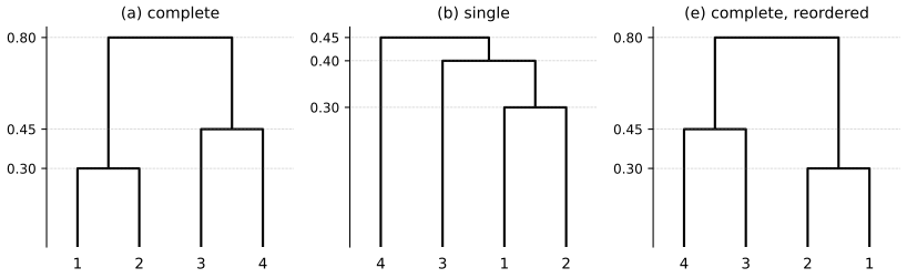
Exercise 2: complete linkage (a), single linkage (b), and the tree of (a) with both fusions swapped (e). Download: PDF · SVG Exercise 12.3. K-means by hand with \(K=2\) on six observations: \((1,4)\), \((1,3)\), \((0,4)\), \((5,1)\), \((6,2)\), \((4,0)\). (a) Plot them. (b) Assign random labels. (c) Compute the centroids. (d) Reassign each observation to the nearest centroid. (e) Repeat (c) and (d) until nothing changes. (f) Colour the plot by the final clusters.
Solution
We take observations 1, 3, 5 in cluster 1 and 2, 4, 6 in cluster 2 as the "random" start (any start gives the same end here). (c) Centroids \((2.33,3.33)\) and \((3.33,1.33)\). (d) Observations 1, 2, 3 are closer to the first, 4, 5, 6 to the second. (e) New centroids \((0.67,3.67)\) and \((5,1)\); the assignments do not change, so the algorithm stops with clusters \(\{1,2,3\}\) and \(\{4,5,6\}\), the two visible groups. (12.17) is \(2\times(1.33+4)=10.67\).
R
# -- [E3] Exercise 3: K-means by hand, K = 2, from a fixed starting assignment
step("E3", "Exercise 3")
x3 <- cbind(c(1, 1, 0, 5, 6, 4), c(4, 3, 4, 1, 2, 0))
lab <- c(1, 2, 1, 2, 1, 2)             # observations 1, 3, 5 start in cluster 1
repeat {
  cent <- rbind(colMeans(x3[lab == 1, , drop = FALSE]), colMeans(x3[lab == 2, , drop = FALSE]))
  print(cent)
  d1 <- rowSums(sweep(x3, 2, cent[1, ])^2)
  d2 <- rowSums(sweep(x3, 2, cent[2, ])^2)
  new <- ifelse(d1 <= d2, 1, 2)
  print(new)
  if (all(new == lab)) break
  lab <- new
}
Python
# -- [E3] Exercise 3: K-means by hand, K = 2, from a fixed starting assignment
step("E3", "Exercise 3")
x3 = np.array([[1, 4], [1, 3], [0, 4], [5, 1], [6, 2], [4, 0]], float)
lab = np.array([1, 2, 1, 2, 1, 2])                # observations 1, 3, 5 start in cluster 1
while True:
    cent = np.array([x3[lab == k].mean(0) for k in (1, 2)])
    print(cent.round(5).tolist())
    new = np.where(((x3 - cent[0]) ** 2).sum(1) <= ((x3 - cent[1]) ** 2).sum(1), 1, 2)
    print(new)
    if np.array_equal(new, lab):
        break
    lab = new
R output
        [,1]    [,2]
[1,] 2.33333 3.33333
[2,] 3.33333 1.33333
[1] 1 1 1 2 2 2
         [,1]    [,2]
[1,] 0.666667 3.66667
[2,] 5.000000 1.00000
[1] 1 1 1 2 2 2
Python output
[[2.33333, 3.33333], [3.33333, 1.33333]]
[1 1 1 2 2 2]
[[0.66667, 3.66667], [5.0, 1.0]]
[1 1 1 2 2 2]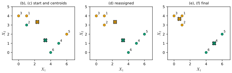
Exercise 3: the start and its centroids, the first reassignment, and the final clusters (the crosses are the centroids). Download: PDF · SVG Exercise 12.4. Single- and complete-linkage dendrograms of the same data. (a) Clusters \(\{1,2,3\}\) and \(\{4,5\}\) fuse in both: which fusion is higher? (b) The same for \(\{5\}\) and \(\{6\}\).
Solution
(a) The single-linkage height is the smallest of the six dissimilarities \(d_{ij}\), \(i\in\{1,2,3\}\), \(j\in\{4,5\}\); the complete-linkage height is the largest. So the complete-linkage fusion is at least as high, and strictly higher unless all six dissimilarities are equal. Without the data one cannot rule out that tie, so strictly "not enough information", but complete is never lower. (b) Both linkages give \(d_{56}\) for two single observations: the same height.
Exercise 12.5. Describe the K-means clusters (\(K=2\)) of the eight shoppers of Figure 12.16 for each of the three scalings.
Solution
Raw counts: socks vary over a range of 6 pairs and computers by at most 1, so socks dominate the distances and the clusters are "many socks" against "few socks", ignoring computers. With our numbers: shoppers 1, 2, 8 (8, 11 and 9 pairs) against the rest. Scaled by the standard deviations (1.92 for socks, 0.53 for computers): one computer is now worth almost two standard deviations, and the clusters are the four computer buyers against the four others. Dollars: a computer costs 1500 dollars and a pair of socks 3, so the clusters are again computer buyers against the rest, now with socks playing no role at all. (Checked numerically with K-means on our eight shoppers.)
Exercise 12.6. Suppose the first \(M\) score vectors \(\bz_1,\dots,\bz_M\) are known. Using (12.6), explain why the loading vectors can be found by separate least-squares regressions, one feature of the data matrix being the response in each and the score vectors the predictors.
Solution
With \(\bA=\bZ_M\) fixed, (12.6) is \(\sum_{j=1}^p\|X_j-\bZ_M b_j\|^2\), where \(X_j\) is column \(j\) of \(\bX\) and \(b_j=(b_{j1},\dots,b_{jM})^\T\) is row \(j\) of \(\bB\). The terms involve disjoint unknowns, so each is minimised separately: \(b_j\) is the least-squares coefficient vector of the regression of \(X_j\) on \(\bz_1,\dots,\bz_M\) (no intercept, the data being centred). There are \(p\) such regressions, one per feature (not \(M\): Note 3). Since the score vectors are orthogonal with \(\bz_m^\T\bz_m=d_m^2\), the solution is \(b_{jm}=\bz_m^\T X_j/d_m^2\), and \(\bX^\T\bz_m=\bX^\T\bX\bphi_m=d_m^2\bphi_m\) gives \(b_{jm}=\phi_{jm}\): the regressions return the loadings.
Exercise 12.7. Show on USArrests that, after standardising each observation, \(1-r_{ij}\) is proportional to the squared Euclidean distance between observations \(i\) and \(j\).
Solution
Standardising each state across its four values, the ratio of squared distance to \(1-r\) is exactly \(2(p-1)=6\) for all 1,225 pairs (Result 12.10). If instead the variables are standardised, as usual, the ratio varies from 0.2 to 11,670: the proportionality needs row standardisation.
R
# -- [E7] Exercise 7: correlation-based against squared Euclidean distance
step("E7", "Exercise 7")
xs <- t(scale(t(as.matrix(USArrests))))   # each STATE centred and scaled across its 4 values
d7 <- as.matrix(dist(xs))^2
r7 <- cor(t(xs))
ratio <- d7[upper.tri(d7)] / (1 - r7[upper.tri(r7)])
summary(ratio)                          # constant 2 (p - 1) = 6
xc <- scale(USArrests)                  # columns scaled only: not proportional
dc <- as.matrix(dist(xc))^2
rc <- cor(t(xc))
summary(dc[upper.tri(dc)] / (1 - rc[upper.tri(rc)]))
Python
# -- [E7] Exercise 7: correlation-based against squared Euclidean distance
step("E7", "Exercise 7")
A = USArrests.to_numpy(float)
xs = (A - A.mean(1, keepdims=True)) / A.std(1, ddof=1, keepdims=True)   # each STATE standardised
iu = np.triu_indices(50, 1)
d7 = ((xs[:, None, :] - xs[None, :, :]) ** 2).sum(2)[iu]
r7 = np.corrcoef(xs)[iu]
print(pd.Series(d7 / (1 - r7)).describe().round(4).to_dict())     # constant 2 (p - 1) = 6
xc = (A - A.mean(0)) / A.std(0, ddof=1)                            # columns scaled only
dc = ((xc[:, None, :] - xc[None, :, :]) ** 2).sum(2)[iu]
print(pd.Series(dc / (1 - np.corrcoef(xc)[iu])).describe().round(2).to_dict())
R output
   Min. 1st Qu.  Median    Mean 3rd Qu.    Max.
      6       6       6       6       6       6
    Min.  1st Qu.   Median     Mean  3rd Qu.     Max.
    0.20     3.81     7.47    35.72    14.46 11670.38
Python output
{'count': 1225.0, 'mean': 6.0, 'std': 0.0, 'min': 6.0, '25%': 6.0, '50%': 6.0, '75%': 6.0, 'max': 6.0}
{'count': 1225.0, 'mean': 35.72, 'std': 367.87, 'min': 0.2, '25%': 3.81, '50%': 7.47, '75%': 14.46, 'max': 11670.38}
Exercise 12.8. Compute the PVE of the USArrests components (a) from the output of the PCA (
sdev,explained_variance_ratio_) and (b) directly from (12.10) with the loadings.Solution
Both give 0.62006, 0.24744, 0.08914, 0.04336, as they must by Result 12.3(b), provided (12.10) is applied to the same centred and scaled data.
R
# -- [E8] Exercise 8: the PVE from sdev and directly from (12.10)
step("E8", "Exercise 8")
pr8 <- prcomp(USArrests, scale = TRUE)
pve.a <- pr8$sdev^2 / sum(pr8$sdev^2)
Xs <- scale(USArrests)
pve.b <- colSums((Xs %*% pr8$rotation)^2) / sum(Xs^2)
rbind(pve.a, pve.b)
Python
# -- [E8] Exercise 8: the PVE from the fitted PCA and directly from (12.10)
step("E8", "Exercise 8")
pca8 = PCA().fit(USArrests_scaled)
pve_b = ((USArrests_scaled @ pca8.components_.T) ** 2).sum(0) / (USArrests_scaled ** 2).sum()
print(np.vstack([pca8.explained_variance_ratio_, pve_b]).round(6))
R output
          PC1      PC2       PC3       PC4
pve.a 0.62006 0.247441 0.0891408 0.0433575
pve.b 0.62006 0.247441 0.0891408 0.0433575
Python output
[[0.62006  0.247441 0.089141 0.043358]
 [0.62006  0.247441 0.089141 0.043358]]
Exercise 12.9. Hierarchically cluster the states with complete linkage and Euclidean distance; cut into three clusters; repeat after scaling the variables; what does scaling change, and should one scale?
Solution
Unscaled, the three clusters are essentially three levels of Assault (cluster means 272.6, 173.3 and 87.6 assaults per 100,000, with 16, 14 and 20 states), because Assault's variance dwarfs the others. After scaling, all four variables count and the clusters change (cross-tabulation below): the 20 low-Assault states of unscaled cluster 3 stay together but are joined by 11 others, while unscaled clusters 1 and 2 are reshuffled, urbanisation and rape now separating states with similar assault rates. Since the variables are in different units (counts per 100,000 and a percentage), scaling is the sensible choice here.
R
# -- [E9] Exercise 9: hierarchical clustering of the states, unscaled and scaled
step("E9", "Exercise 9")
hc9 <- hclust(dist(USArrests), method = "complete")
c9 <- cutree(hc9, 3)
split(state.abb, c9)
hc9s <- hclust(dist(scale(USArrests)), method = "complete")
c9s <- cutree(hc9s, 3)
table(unscaled = c9, scaled = c9s)
round(sapply(split(as.data.frame(USArrests), c9), colMeans), 1)
Python
# -- [E9] Exercise 9: hierarchical clustering of the states, unscaled and scaled
step("E9", "Exercise 9")
abb = ["AL", "AK", "AZ", "AR", "CA", "CO", "CT", "DE", "FL", "GA", "HI", "ID", "IL", "IN", "IA", "KS", "KY",
       "LA", "ME", "MD", "MA", "MI", "MN", "MS", "MO", "MT", "NE", "NV", "NH", "NJ", "NM", "NY", "NC", "ND",
       "OH", "OK", "OR", "PA", "RI", "SC", "SD", "TN", "TX", "UT", "VT", "VA", "WA", "WV", "WI", "WY"]
c9 = cut_tree(linkage(A, "complete"), n_clusters=3).ravel()
for k in range(3):
    print(k + 1, [a for a, c in zip(abb, c9) if c == k])
c9s = cut_tree(linkage(xc, "complete"), n_clusters=3).ravel()
print(pd.crosstab(pd.Series(c9 + 1, name="unscaled"), pd.Series(c9s + 1, name="scaled")))
print(USArrests.groupby(c9 + 1).mean().T.round(1))
R output
$`1`
 [1] "AL" "AK" "AZ" "CA" "DE" "FL" "IL" "LA" "MD" "MI" "MS" "NV" "NM" "NY" "NC" "SC"

$`2`
 [1] "AR" "CO" "GA" "MA" "MO" "NJ" "OK" "OR" "RI" "TN" "TX" "VA" "WA" "WY"

$`3`
 [1] "CT" "HI" "ID" "IN" "IA" "KS" "KY" "ME" "MN" "MT" "NE" "NH" "ND" "OH" "PA" "SD" "UT" "VT" "WV"
[20] "WI"

        scaled
unscaled  1  2  3
       1  6  9  1
       2  2  2 10
       3  0  0 20
             1     2    3
Murder    11.8   8.2  4.3
Assault  272.6 173.3 87.6
UrbanPop  68.3  70.6 59.8
Rape      28.4  22.8 14.4
Python output
1 ['AL', 'AK', 'AZ', 'CA', 'DE', 'FL', 'IL', 'LA', 'MD', 'MI', 'MS', 'NV', 'NM', 'NY', 'NC', 'SC']
2 ['AR', 'CO', 'GA', 'MA', 'MO', 'NJ', 'OK', 'OR', 'RI', 'TN', 'TX', 'VA', 'WA', 'WY']
3 ['CT', 'HI', 'ID', 'IN', 'IA', 'KS', 'KY', 'ME', 'MN', 'MT', 'NE', 'NH', 'ND', 'OH', 'PA', 'SD', 'UT', 'VT', 'WV', 'WI']
scaled    1  2   3
unscaled
1         6  9   1
2         2  2  10
3         0  0  20
              1      2     3
Murder     11.8    8.2   4.3
Assault   272.6  173.3  87.6
UrbanPop   68.3   70.6  59.8
Rape       28.4   22.8  14.4
Exercise 12.10. Simulate 20 observations in each of three classes on 50 variables with mean shifts; (b) plot the first two principal component scores; K-means with (c) \(K=3\), (d) \(K=2\), (e) \(K=4\), (f) \(K=3\) on the first two score vectors, (g) \(K=3\) after scaling each variable.
Solution
Class 2 is shifted by \(+1.2\) on the first 25 variables and class 3 by \(-1.2\) on the last 25. The first two components explain 19.3% and 10.7% of the variance and separate the classes well. (c) K-means with \(K=3\) recovers the classes except for one observation of class 1. (d) With \(K=2\), classes 1 and 3 are merged (apart from that observation). (e) With \(K=4\), one class is split in two: class 3 (11 and 9) in R, class 2 (4 and 16) in Python, two local optima of nearly equal quality; this is the one place where the two languages differ. (f) On the first two score vectors, the same clusters as (c): the class structure lives in those two dimensions. (g) After scaling, again the same: the variables already have similar spreads.
R
# -- [E10] Exercise 10: three simulated classes, PCA and K-means
step("E10", "Exercise 10")
I10 <- matrix(rep(1:60, 50), 60)
J10 <- matrix(rep(1:50, each = 60), 60)
x10 <- qnorm(hash_u(I10, J10, 10))      # 60 x 50 "standard normal" values
cls <- rep(1:3, each = 20)
x10[cls == 2, 1:25] <- x10[cls == 2, 1:25] + 1.2    # class 2 shifted up on the first 25 variables
x10[cls == 3, 26:50] <- x10[cls == 3, 26:50] - 1.2  # class 3 shifted down on the last 25
pr10 <- prcomp(x10)
round(summary(pr10)$importance[2, 1:3], 4)
pdf(file.path(img_dir, "lab-r-ex10.pdf"), width = 4.5, height = 4.2)
plot(pr10$x[, 1:2], col = cls + 1, pch = 19, xlab = "Z1", ylab = "Z2")
invisible(dev.off())
set.seed(10)
table(cls, kmeans(x10, 3, nstart = 20)$cluster)
table(cls, kmeans(x10, 2, nstart = 20)$cluster)
table(cls, kmeans(x10, 4, nstart = 20)$cluster)
table(cls, kmeans(pr10$x[, 1:2], 3, nstart = 20)$cluster)
table(cls, kmeans(scale(x10), 3, nstart = 20)$cluster)
Python
# -- [E10] Exercise 10: three simulated classes, PCA and K-means
step("E10", "Exercise 10")
I10, J10 = np.meshgrid(np.arange(1, 61), np.arange(1, 51), indexing="ij")
x10 = norm.ppf(hash_u(I10, J10, 10))          # the same 60 x 50 values as the R lab
cls = np.repeat([1, 2, 3], 20)
x10[cls == 2, :25] += 1.2
x10[cls == 3, 25:] -= 1.2
pca10 = PCA().fit(x10)
z10 = pca10.transform(x10)
print(pca10.explained_variance_ratio_[:3].round(4))
fig, ax = plt.subplots(figsize=(4.5, 4.2))
ax.scatter(z10[:, 0], z10[:, 1], c=cls, cmap="brg", s=25)
ax.set_xlabel("PC1"); ax.set_ylabel("PC2")
savefig(fig, 12, "lab-py-ex10")
for data, K in ((x10, 3), (x10, 2), (x10, 4), (z10[:, :2], 3), (StandardScaler().fit_transform(x10), 3)):
    km = KMeans(n_clusters=K, n_init=20, random_state=10).fit(data)
    print(pd.crosstab(pd.Series(cls, name="cls"), km.labels_ + 1).to_string())
R output
   PC1    PC2    PC3
0.1933 0.1072 0.0445

cls  1  2  3
  1  0  1 19
  2  0 20  0
  3 20  0  0

cls  1  2
  1 19  1
  2  0 20
  3 20  0

cls  1  2  3  4
  1  0 19  1  0
  2  0  0 20  0
  3 11  0  0  9

cls  1  2  3
  1  1 19  0
  2 20  0  0
  3  0  0 20

cls  1  2  3
  1  1  0 19
  2 20  0  0
  3  0 20  0
Python output
[0.1933 0.1072 0.0444]
col_0   1   2   3
cls
1       0   1  19
2       0  20   0
3      20   0   0
col_0   1   2
cls
1      19   1
2       0  20
3      20   0
col_0   1  2   3   4
cls
1      19  0   0   1
2       0  4   0  16
3       0  0  20   0
col_0   1   2   3
cls
1       0   1  19
2       0  20   0
3      20   0   0
col_0   1   2   3
cls
1       0   1  19
2       0  20   0
3      20   0   0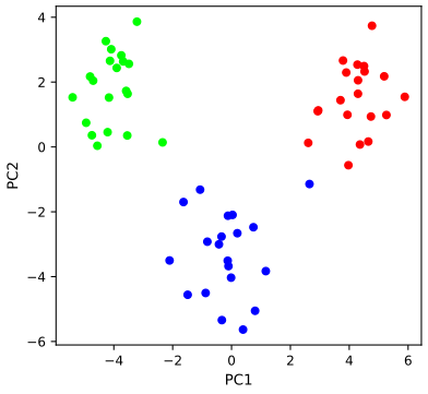
Exercise 10: the first two score vectors of the simulated data, coloured by class. Download: PDF · SVG Exercise 12.11. Write a matrix-completion function (Algorithm 12.1) with a relative-error stopping rule, a maximum number of iterations and an option to print progress. On the standardised Boston data, hide nested sets of 5%, 10%, ..., 30% of the entries, run the algorithm with \(M=1,\dots,8\), and plot the error averaged over 10 repetitions.
Solution
The error is the mean squared difference between imputed and true values on the hidden entries (the data are standardised, so column-mean imputation would give about 1). With \(M=1\) to 3 it is about 0.52–0.71, best at \(M=3\) when few entries are missing and at \(M=1\) when many are; it grows with the fraction missing for \(M=2,3\), whose extra components are fitted to fewer observed values. From \(M=4\) on the error jumps above 1.7, worse than mean imputation: hard impute with many components overfits the observed entries and extrapolates wildly into the hidden ones, the effect seen with \(M=2\) on USArrests in the demonstration. Both languages give the same table (the hidden sets come from the shared formula).
R
# -- [E11] Exercise 11: a matrix completion function, tested on the Boston data
step("E11", "Exercise 11")
mat_complete <- function(Xna, M = 1, thresh = 1e-7, maxit = 500, verbose = FALSE) {
  ismiss <- is.na(Xna)
  xbar <- colMeans(Xna, na.rm = TRUE)
  Xhat <- Xna
  Xhat[ismiss] <- matrix(xbar, nrow(Xna), ncol(Xna), byrow = TRUE)[ismiss]
  mss0 <- mean(Xna[!ismiss]^2)
  mssold <- mean((scale(Xna, xbar, FALSE)[!ismiss])^2)
  rel_err <- 1
  iter <- 0
  while (rel_err > thresh && iter < maxit) {
    iter <- iter + 1
    Xapp <- fit.svd(Xhat, M)
    Xhat[ismiss] <- Xapp[ismiss]
    mss <- mean(((Xna - Xapp)[!ismiss])^2)
    rel_err <- (mssold - mss) / mss0
    mssold <- mss
    if (verbose) cat("Iter:", iter, "MSS:", mss, "Rel. Err:", rel_err, "\n")
  }
  list(Xhat = Xhat, iter = iter, mss = mss)
}
XB <- scale(as.matrix(Boston))
N <- length(XB)
fracs <- seq(0.05, 0.30, by = 0.05)
err <- array(0, c(10, length(fracs), 8))
for (r in 1:10) {
  ord <- order(hash_u(seq_len(N), 0, 100 + r))   # a fixed random order of the entries; nested sets
  for (a in seq_along(fracs)) {
    miss <- ord[seq_len(round(fracs[a] * N))]
    Xna <- XB
    Xna[miss] <- NA
    for (M in 1:8) {
      fit <- mat_complete(Xna, M)
      err[r, a, M] <- mean((fit$Xhat[miss] - XB[miss])^2)
    }
  }
}
E11 <- apply(err, c(2, 3), mean)
dimnames(E11) <- list(paste0(100 * fracs, "%"), paste0("M=", 1:8))
round(E11, 3)
Python
# -- [E11] Exercise 11: a matrix completion function, tested on the Boston data
step("E11", "Exercise 11")


def mat_complete(Xna, M=1, thresh=1e-7, maxit=500, verbose=False):
    ismiss = np.isnan(Xna)
    xbar = np.nanmean(Xna, 0)
    Xhat = np.where(ismiss, xbar, Xna)
    mss0 = np.mean(Xna[~ismiss] ** 2)
    mssold = np.mean((Xna - xbar)[~ismiss] ** 2)
    rel_err, it = 1.0, 0
    while rel_err > thresh and it < maxit:
        it += 1
        Xapp = low_rank(Xhat, M)
        Xhat[ismiss] = Xapp[ismiss]
        mss = np.mean(((Xna - Xapp)[~ismiss]) ** 2)
        rel_err = (mssold - mss) / mss0
        mssold = mss
        if verbose:
            print("Iter:", it, "MSS:", mss, "Rel. Err:", rel_err)
    return Xhat, it, mss


Boston = isl_data("Boston", index_col=0)
XB = Boston.to_numpy(float)
XB = (XB - XB.mean(0)) / XB.std(0, ddof=1)
N = XB.size
fracs = np.arange(1, 7) * 0.05
err = np.zeros((10, 6, 8))
for r in range(1, 11):
    order = np.argsort(hash_u(np.arange(1, N + 1), 0, 100 + r), kind="stable")   # R's column-major order
    for a, f in enumerate(fracs):
        miss = order[:int(round(f * N))]
        rows, cols = miss % XB.shape[0], miss // XB.shape[0]
        Xna = XB.copy()
        Xna[rows, cols] = np.nan
        for M in range(1, 9):
            Xhat, _, _ = mat_complete(Xna, M)
            err[r - 1, a, M - 1] = np.mean((Xhat[rows, cols] - XB[rows, cols]) ** 2)
E11 = pd.DataFrame(err.mean(0), index=["%d%%" % round(100 * f) for f in fracs],
                   columns=["M=%d" % M for M in range(1, 9)])
print(E11.round(3))
fig, ax = plt.subplots(figsize=(5.5, 3.8))
for M in range(1, 9):
    ax.plot(100 * fracs, E11.iloc[:, M - 1], marker="o", label="M = %d" % M)
ax.axhline(1, color=GREY, ls=":", lw=1)
ax.set_yscale("log"); ax.set_xlabel("% of entries missing"); ax.set_ylabel("mean squared error, missing entries")
ax.legend(fontsize=7, ncol=2)
savefig(fig, 12, "lab-py-ex11")
R output
      M=1   M=2   M=3   M=4   M=5   M=6   M=7   M=8
5%  0.596 0.563 0.517 1.717 3.867 4.286 3.861 5.226
10% 0.604 0.573 0.539 2.318 3.278 3.976 3.802 4.152
15% 0.605 0.584 0.567 2.422 3.327 3.341 3.459 3.956
20% 0.603 0.592 0.620 2.378 3.072 3.381 3.489 3.846
25% 0.598 0.606 0.674 2.426 2.988 3.386 3.467 3.560
30% 0.607 0.634 0.710 2.595 2.860 3.576 3.368 3.366
Python output
       M=1    M=2    M=3    M=4    M=5    M=6    M=7    M=8
5%   0.596  0.563  0.517  1.717  3.867  4.286  3.861  5.226
10%  0.604  0.573  0.539  2.318  3.278  3.976  3.802  4.152
15%  0.605  0.584  0.567  2.422  3.327  3.341  3.459  3.956
20%  0.603  0.592  0.620  2.378  3.072  3.381  3.489  3.846
25%  0.598  0.606  0.674  2.426  2.988  3.386  3.467  3.560
30%  0.607  0.634  0.710  2.595  2.860  3.576  3.368  3.366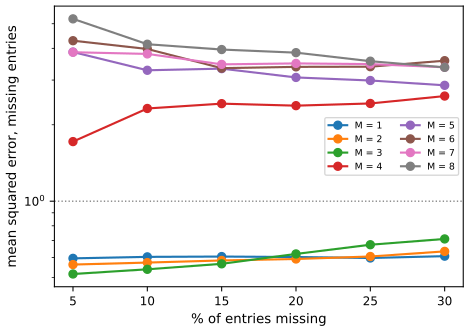
Exercise 11: mean squared imputation error on the hidden entries of the standardised Boston data, averaged over 10 repetitions, for \(M=1,\dots,8\); the dotted line is the error of column-mean imputation. Download: PDF · SVG Exercise 12.12. Implement Algorithm 12.1 with
prcomp()(R) orPCA()(Python) instead of the SVD.Solution
prcomp(X, center = FALSE)gives exactly the SVD fit, so the algorithm is unchanged (correlation 0.653504 on the lab's entries). With centring (the default ofprcomp(), and always the case for scikit-learn'sPCA()), the reconstructioninverse_transformadds back the column means: the fit becomes "column means plus rank \(M\)", a slightly different model, and the correlation becomes 0.653040. Both languages agree.R
# -- [E12] Exercise 12: Algorithm 12.1 with prcomp() in place of svd()
step("E12", "Exercise 12")
fit.pca <- function(X, M = 1, center = FALSE) {
  p <- prcomp(X, center = center, scale. = FALSE)
  app <- p$x[, 1:M, drop = FALSE] %*% t(p$rotation[, 1:M, drop = FALSE])
  if (center) sweep(app, 2, p$center, "+") else app
}
impute_with <- function(fitfun, Xna, M = 1) {
  ismiss <- is.na(Xna)
  xbar <- colMeans(Xna, na.rm = TRUE)
  Xhat <- Xna
  Xhat[ismiss] <- matrix(xbar, nrow(Xna), ncol(Xna), byrow = TRUE)[ismiss]
  mss0 <- mean(Xna[!ismiss]^2)
  mssold <- mean((scale(Xna, xbar, FALSE)[!ismiss])^2)
  rel_err <- 1
  while (rel_err > 1e-7) {
    Xapp <- fitfun(Xhat, M)
    Xhat[ismiss] <- Xapp[ismiss]
    mss <- mean(((Xna - Xapp)[!ismiss])^2)
    rel_err <- (mssold - mss) / mss0
    mssold <- mss
  }
  Xhat
}
Xna <- X
Xna[index.na] <- NA
c(svd = cor(impute_with(fit.svd, Xna)[ismiss], X[ismiss]),
  prcomp = cor(impute_with(function(X, M) fit.pca(X, M), Xna)[ismiss], X[ismiss]),
  prcomp.centred = cor(impute_with(function(X, M) fit.pca(X, M, TRUE), Xna)[ismiss], X[ismiss]))
Python
# -- [E12] Exercise 12: Algorithm 12.1 with PCA() in place of the SVD
step("E12", "Exercise 12")


def fit_pca(X, M=1):
    """PCA() centres the columns, so its rank-M reconstruction is mean + rank-M (an affine fit)."""
    p = PCA(n_components=M).fit(X)
    return p.inverse_transform(p.transform(X))


def impute_with(fitfun, Xna, M=1):
    ismiss = np.isnan(Xna)
    xbar = np.nanmean(Xna, 0)
    Xhat = np.where(ismiss, xbar, Xna)
    mss0 = np.mean(Xna[~ismiss] ** 2)
    mssold = np.mean((Xna - xbar)[~ismiss] ** 2)
    rel_err = 1.0
    while rel_err > 1e-7:
        Xapp = fitfun(Xhat, M)
        Xhat[ismiss] = Xapp[ismiss]
        mss = np.mean(((Xna - Xapp)[~ismiss]) ** 2)
        rel_err = (mssold - mss) / mss0
        mssold = mss
    return Xhat


print({"svd": round(np.corrcoef(impute_with(low_rank, XRna)[ina, inb], XR[ina, inb])[0, 1], 6),
       "PCA (centred)": round(np.corrcoef(impute_with(fit_pca, XRna)[ina, inb], XR[ina, inb])[0, 1], 6)})
R output
           svd         prcomp prcomp.centred
      0.653504       0.653504       0.653040
Python output
{'svd': 0.653504, 'PCA (centred)': 0.65304}Exercise 12.13. The file Ch12Ex13.csv holds 1,000 genes (rows) for 40 tissue samples (columns): 20 healthy, then 20 diseased. (b) Cluster the samples hierarchically with correlation-based distance; do they separate into the two groups, and does it depend on the linkage? (c) Which genes differ most between the groups?
Solution
(b) With complete or average linkage the 20 diseased samples all fall in one cluster, but so do about half of the healthy ones: the separation is partial. Single linkage puts one sample on its own and everything else together. So the answer depends on the linkage, and correlation-based clustering alone does not separate the groups cleanly. (c) A two-sample (Welch) \(t\)-test for each gene, with a Bonferroni correction for the 1,000 tests (threshold \(0.05/1000\)), flags 105 genes: 95 of genes 501–600 and genes 11–20. The genes with the largest \(|t|\) are all in 501–600, which is where the diseased samples' expression is shifted (mean 2.03 against 0.00). The false discovery rate of Chapter 13 would be a less conservative alternative to Bonferroni.
R
# -- [E13] Exercise 13: gene expression of 40 tissue samples (20 healthy, 20 diseased)
step("E13", "Exercise 13")
g13 <- read.csv(file.path(.this_dir, "isl-data", "Ch12Ex13.csv"), header = FALSE)
dim(g13)                               # 1000 genes (rows) x 40 samples (columns)
dcor <- as.dist(1 - cor(g13))          # correlation between samples
grp <- rep(1:2, each = 20)
for (m in c("complete", "average", "single")) {
  cat(m, ":", cutree(hclust(dcor, method = m), 2), "\n")
}
tt <- apply(g13, 1, function(g) t.test(g[1:20], g[21:40])$statistic)
pv <- apply(g13, 1, function(g) t.test(g[1:20], g[21:40])$p.value)
sum(pv < 0.05 / 1000)                  # genes significant after a Bonferroni correction
head(order(-abs(tt)), 10)              # the ten genes with the largest |t|
range(which(pv < 0.05 / 1000))
Python
# -- [E13] Exercise 13: gene expression of 40 tissue samples (20 healthy, 20 diseased)
step("E13", "Exercise 13")
g13 = isl_data("Ch12Ex13", header=None).to_numpy(float)
print(g13.shape)                               # 1000 genes (rows) x 40 samples (columns)
dcor = 1 - np.corrcoef(g13.T)                  # correlation between samples
iu = np.triu_indices(40, 1)
for m in ("complete", "average", "single"):
    print(m, ":", cut_tree(linkage(dcor[iu], method=m), n_clusters=2).ravel() + 1)
t13, p13 = ttest_ind(g13[:, :20], g13[:, 20:], axis=1, equal_var=False)
print((p13 < 0.05 / 1000).sum())               # genes significant after a Bonferroni correction
print(np.argsort(-np.abs(t13))[:10] + 1)       # the ten genes with the largest |t|
print(np.flatnonzero(p13 < 0.05 / 1000)[[0, -1]] + 1)
R output
[1] 1000   40
complete : 1 2 1 1 2 1 2 1 2 2 1 1 2 1 1 2 2 2 2 1 2 2 2 2 2 2 2 2 2 2 2 2 2 2 2 2 2 2 2 2
average : 1 1 1 1 2 2 1 2 1 2 2 2 2 2 2 1 2 2 1 1 2 2 2 2 2 2 2 2 2 2 2 2 2 2 2 2 2 2 2 2
single : 1 1 1 1 1 1 1 1 1 1 1 1 1 1 1 1 1 1 2 1 1 1 1 1 1 1 1 1 1 1 1 1 1 1 1 1 1 1 1 1
[1] 105
 [1] 502 589 600 590 565 551 593 584 538 569
[1]  11 600
Python output
(1000, 40)
complete : [1 2 1 1 2 1 2 1 2 2 1 1 2 1 1 2 2 2 2 1 2 2 2 2 2 2 2 2 2 2 2 2 2 2 2 2 2 2 2 2]
average : [1 1 1 1 2 2 1 2 1 2 2 2 2 2 2 1 2 2 1 1 2 2 2 2 2 2 2 2 2 2 2 2 2 2 2 2 2 2 2 2]
single : [1 1 1 1 1 1 1 1 1 1 1 1 1 1 1 1 1 1 2 1 1 1 1 1 1 1 1 1 1 1 1 1 1 1 1 1 1 1 1 1]
105
[502 589 600 590 565 551 593 584 538 569]
[ 11 600]
Demonstrations for this chapter
Each demonstration runs in the browser on the book's data and links back to these notes. The ▶ Demo boxes above open them already set to the case under discussion.
| Demonstration | What you can see | Sections |
|---|---|---|
| PCA of the USArrests data: scaling, units and signs | The biplot, the PVE and the loadings with the variables standardised or not, Assault counted per 100,000, 10,000, 1,000 or 100 people, any two of the four components, and the signs of the book, of prcomp() and of scikit-learn. Presets: 1 Figure 12.1; 2 unscaled; 3 unscaled, Assault per 100 people; 4 the same standardised; 5 prcomp()'s signs. | 12.2.1, 12.2.3, 12.2.4 |
| Matrix completion by iterated principal components | Algorithm 12.1 on the standardised USArrests data, one iteration at a time: imputed against true values, the objective (12.14) on the observed entries, and the error on the hidden ones against mean imputation and the complete-data approximation. Presets: 1 the R lab; 2 the Python lab; 3 step by step; 4 \(M=2\); 5 a value hidden in every state. | 12.3, 12.5.2 |
| K-means against hierarchical clustering: nested or not | The clusters of K-means and of a cut dendrogram side by side for \(K=1\) to 8, with (12.17) for both, the adjusted Rand index between them, and whether each K-means solution is nested in the previous one; four linkages (with the inversions of centroid linkage) and four data sets. Presets: 1 men and women, \(K=2\); 2 \(K=3\); 3 NCI60 scores, \(K=4\); 4 USArrests, average linkage; 5 single linkage chaining. | 12.4.1, 12.4.2, 12.5.4 |
Related demonstrations in the companion courses: the PCA explorer, the SVD and the best rank-k approximation, k-means, k-medoids and PAM step by step, linkages and dendrograms and how many clusters? in Statistical Methods for Modern Biology; spectral clustering in Statistical Learning: Theory and Methods; K-means and EM and PCA and probabilistic PCA in Bayesian and Probabilistic Machine Learning.
References
- James, G., Witten, D., Hastie, T. and Tibshirani, R. (2021). An Introduction to Statistical Learning with Applications in R, 2nd edition. Springer, New York. Chapter 12, pp. 497–552. www.statlearning.com.
- James, G., Witten, D., Hastie, T., Tibshirani, R. and Taylor, J. (2023). An Introduction to Statistical Learning with Applications in Python. Springer, Cham. Chapter 12.
- Eckart, C. and Young, G. (1936). The approximation of one matrix by another of lower rank. Psychometrika, 1, 211–218.
- Hartigan, J. A. and Wong, M. A. (1979). Algorithm AS 136: a K-means clustering algorithm. Journal of the Royal Statistical Society, Series C, 28, 100–108.
- Hastie, T., Tibshirani, R. and Friedman, J. (2009). The Elements of Statistical Learning, 2nd edition. Springer, New York. Chapter 14.
- Hotelling, H. (1933). Analysis of a complex of statistical variables into principal components. Journal of Educational Psychology, 24, 417–441.
- Jolliffe, I. T. (2002). Principal Component Analysis, 2nd edition. Springer, New York.
- Kaufman, L. and Rousseeuw, P. J. (1990). Finding Groups in Data: An Introduction to Cluster Analysis. Wiley, New York.
- Lloyd, S. P. (1982). Least squares quantization in PCM. IEEE Transactions on Information Theory, 28, 129–137.
- MacQueen, J. (1967). Some methods for classification and analysis of multivariate observations. Proceedings of the Fifth Berkeley Symposium on Mathematical Statistics and Probability, 1, 281–297.
- Mazumder, R., Hastie, T. and Tibshirani, R. (2010). Spectral regularization algorithms for learning large incomplete matrices. Journal of Machine Learning Research, 11, 2287–2322.
- Pearson, K. (1901). On lines and planes of closest fit to systems of points in space. Philosophical Magazine, 2, 559–572.
- Ross, D. T. et al. (2000). Systematic variation in gene expression patterns in human cancer cell lines. Nature Genetics, 24, 227–235.
The numerical statements in the text (Table 12.1 and the PVEs, the variance decomposition and the low-rank approximation, the matrix-completion runs and their monotone objectives, the K-means identity, the linkage heights and the men-and-women example, the agreement of the R and Python labs, and the exercise results) were confirmed numerically.