Linear Regression
Linear regression predicts a number from one or more inputs with a straight line, a plane, or a sum of simple terms. It is old, but it is the base on which most of the book is built, and it is the place to learn the questions every model must answer: is there any relationship at all, how strong is it, which inputs matter, how precise are the estimates and the predictions, and when do the assumptions fail. This chapter answers them on the Advertising data, adds qualitative inputs, interactions and curved terms, shows how to read residual plots, leverage and the variance inflation factor, and ends by comparing linear regression with K-nearest neighbours. Every formula the book quotes without proof is derived here, and the lab runs in R and in Python side by side.
Ch. 1 Introduction Ch. 2 Statistical learning Ch. 3 Linear regression Ch. 4 Classification Ch. 5 Resampling Ch. 6 Selection and regularization Ch. 7 Beyond linearity Ch. 8 Trees Ch. 9 SVMs Ch. 10 Deep learning Ch. 11 Survival analysis Ch. 12 Unsupervised learning Ch. 13 Multiple testing
How to read these notes
They follow the book. Sections carry the book's numbers (3.1, 3.2.2, ...) and every displayed equation that appears in the book carries its number, e.g. \((3.4)\); equations without a number are steps the book skips. Page numbers are those of the R edition. A short section before 3.1 collects the seven questions about the Advertising data that the chapter sets out to answer.
Two editions, one course. The R edition (James et al. 2021) and the Python edition (James et al. 2023) share their text, figures and exercises; only the labs differ. Text shared by both is cited as “James et al. (2021), Section …”. The lab (Section 3.6) is given in both languages side by side, and every place where the two languages behave differently is marked by an orange R versus Python note.
Filling the gaps. The book keeps the mathematics light: it says that the least-squares formulas, the standard errors, the F-statistic or the leverage bounds “can be shown”. An orange Filling the gap box gives each argument at the level of a first course in statistics. Derivations start hidden: open one with its bar, or use the button below. Where the graduate course on this site treats a topic in more depth, a Deeper line points to the exact section.
Figures and demonstrations. All twenty figures of the chapter are recomputed by the Python code: eleven from the book's data and nine from simulations whose settings are stated in the captions and in the code. Every table of the chapter is recomputed too. The ▶ Demo boxes open an interactive demonstration already set to the case being discussed.
Main reference
G. James, D. Witten, T. Hastie and R. Tibshirani, An Introduction to Statistical Learning with Applications in R, 2nd edition, Springer (2021), Chapter 3, pages 59–128; and G. James, D. Witten, T. Hastie, R. Tibshirani and J. Taylor, An Introduction to Statistical Learning with Applications in Python, Springer (2023), Chapter 3. Book website, with the data and the official labs: www.statlearning.com. Section, equation, figure, table and exercise numbers below refer to these books.
The explanations, derivations, figures and code are my own; equations are cited by their numbers in the book.
Companion courses
Linear regression is treated from other angles in three companion courses on this site:
- Statistical Learning: Theory and Methods (Hastie, Tibshirani and Friedman 2009, the graduate book by the same authors), Chapter 3: least squares in matrix form and the hat matrix (Section 3.2), the exact sampling distribution behind the t and F tests (Results 3.4 and 3.5), the Gauss–Markov theorem (Section 3.2.2), multiple regression as a sequence of simple regressions (Section 3.2.3) and subset selection (Section 3.3); least squares against nearest neighbours (Section 2.3) and the curse of dimensionality (Section 2.5).
- Bayesian and Probabilistic Machine Learning (Bishop 2006): least squares as maximum likelihood (Section 3.1.1) and its geometry (Section 3.1.2).
- Statistical Methods for Modern Biology (Holmes and Huber 2019), in R: the t-test (Section 6.5), multiple testing (Section 6.7), and linear models with several factors and the analysis of variance (Section 8.7).
New here: the book's data sets (Advertising, Credit, Auto, Boston and Carseats), every number of the chapter's tables recomputed, the R and Python code side by side, and the gentler level of the introductory book.
The chapter at a glance
- 3.1 Simple regression \(Y\approx\beta_0+\beta_1X\). Least squares gives the slope \(\sum(x_i-\bar x)(y_i-\bar y)/\sum(x_i-\bar x)^2\) (Filling the gap 3.1); the estimates are unbiased with standard errors (3.8) (3.2), which give t-based confidence intervals and tests (3.3). The fit is summarised by the RSE and by \(R^2\), which equals the squared correlation (3.4).
- 3.2 Multiple regression. Each coefficient is the effect of its input with the others held fixed, which is why newspaper advertising matters alone but not next to radio (3.5). The F-statistic tests all coefficients at once and is needed because many individual tests produce false alarms (3.6); \(R^2\) is the squared correlation between \(Y\) and the fit (3.7); prediction intervals are wider than confidence intervals by the irreducible error (3.8).
- 3.3 Dummy variables for qualitative inputs (3.9), interactions and the hierarchical principle (3.10), polynomial terms, and six problems: non-linearity, correlated errors (3.12), unequal variances (3.13), outliers, high leverage (3.11) and collinearity (3.14).
- 3.4–3.5 The seven questions answered for the Advertising data; linear regression against K-nearest neighbours, and why KNN suffers as the number of inputs grows (3.15).
- 3.6 The lab, in R and Python: the Boston and Carseats data, with every difference between the two languages marked. Notes on the book lists a swapped pair of coefficients in Table 3.8 and slips in both labs.
Notation. \(n\) observations, \(p\) predictors; \(x_i\) the input of observation \(i\) (a number in simple regression, a vector \((x_{i1},\dots,x_{ip})\) in multiple regression), \(y_i\) its response. \(\bar x\), \(\bar y\) are sample means, \(S_{xx}=\sum_i(x_i-\bar x)^2\), \(S_{yy}=\sum_i(y_i-\bar y)^2\), \(S_{xy}=\sum_i(x_i-\bar x)(y_i-\bar y)\). Hats mark estimates. In matrix form \(\bX\) is the \(n\times(p+1)\) matrix whose rows are \((1,x_{i1},\dots,x_{ip})\), \(\by=(y_1,\dots,y_n)^\T\).
Prerequisites. Chapter 2 of the book (the regression function, the bias–variance trade-off, K-nearest neighbours); means, variances and covariances; the normal and t distributions. The matrix algebra of Section 3.2 uses only products, transposes and inverses.
The seven questions
pp. 59–60 The Advertising data (Chapter 2 of the book) give the sales of a product in \(n=200\) markets, in thousands of units, together with the budgets spent on TV, radio and newspaper advertising in each market, in thousands of dollars. Suppose we must advise on next year's advertising. The chapter is organised around seven questions that such advice needs, and that linear regression answers:
- Is there any relationship between advertising and sales at all?
- If so, how strong is it?
- Which of the three media are associated with sales?
- How large is the association of each medium, and how precisely do we know it?
- How accurately can we predict future sales?
- Is the relationship linear?
- Do the media reinforce each other (a synergy, or in statistical language an interaction)?
The answers are collected in Section 3.4, once the tools have been built.
3.1 Simple Linear Regression
Definition 3.1 (simple linear regression) pp. 61–63, (3.1), (3.2), (3.5)
With one predictor \(X\) and a quantitative response \(Y\), simple linear regression assumes the approximately linear relationship
\[ Y\approx\beta_0+\beta_1X, \tag{3.1} \]read “\(Y\) is regressed on \(X\)”. The unknown constants \(\beta_0\) (the intercept) and \(\beta_1\) (the slope) are the coefficients or parameters. Once they are estimated, a prediction at \(X=x\) is
\[ \hat y=\hat\beta_0+\hat\beta_1x. \tag{3.2} \]As a model for the data, the relationship is written with an explicit error,
\[ Y=\beta_0+\beta_1X+\epsilon, \tag{3.5} \]where \(\epsilon\) has mean zero and is usually assumed independent of \(X\). Equation (3.5) is the population regression line: \(\beta_0\) is the mean of \(Y\) when \(X=0\) and \(\beta_1\) the change in the mean of \(Y\) for a one-unit increase in \(X\).
3.1.1 Estimating the Coefficients
pp. 61–62 From \(n\) pairs \((x_1,y_1),\dots,(x_n,y_n)\) we want a line close to the points. With the prediction \(\hat y_i=\hat\beta_0+\hat\beta_1x_i\), the \(i\)th residual is \(e_i=y_i-\hat y_i\), and the residual sum of squares is
\[ \RSS=e_1^2+e_2^2+\dots+e_n^2=(y_1-\hat\beta_0-\hat\beta_1x_1)^2+\dots+(y_n-\hat\beta_0-\hat\beta_1x_n)^2. \tag{3.3} \]The least-squares line chooses \(\hat\beta_0,\hat\beta_1\) to make RSS as small as possible. The minimisers are
\[ \hat\beta_1=\frac{\sum_{i=1}^n(x_i-\bar x)(y_i-\bar y)}{\sum_{i=1}^n(x_i-\bar x)^2}=\frac{S_{xy}}{S_{xx}},\qquad \hat\beta_0=\bar y-\hat\beta_1\bar x. \tag{3.4} \]On the Advertising data, regressing sales on TV gives \(\hat\beta_0=7.03\) and \(\hat\beta_1=0.0475\): an extra $1,000 of TV advertising goes with about 47.5 more units sold (Figure 3.1).
Filling the gap 3.1: the least-squares estimates (3.4) p. 62, “using some calculus, one can show that the minimizers are”
Setting the two partial derivatives of RSS to zero gives (3.4); an exact identity then shows that it is the unique minimum, that the line passes through \((\bar x,\bar y)\), and that the RSS contours of Figure 3.2 are ellipses.
Derivation
Step 1: the two equations. Treat \(\RSS(b_0,b_1)=\sum_i(y_i-b_0-b_1x_i)^2\) as a function of the candidate intercept and slope. Differentiating,
\[ \frac{\partial\RSS}{\partial b_0}=-2\sum_i(y_i-b_0-b_1x_i),\qquad \frac{\partial\RSS}{\partial b_1}=-2\sum_ix_i(y_i-b_0-b_1x_i). \]The first equals zero when \(\sum_iy_i=nb_0+b_1\sum_ix_i\), that is \(b_0=\bar y-b_1\bar x\). Put this into the second: \(\sum_ix_i\big[(y_i-\bar y)-b_1(x_i-\bar x)\big]=0\), so \(b_1=\sum_ix_i(y_i-\bar y)/\sum_ix_i(x_i-\bar x)\). Since \(\sum_i\bar x(y_i-\bar y)=0\) and \(\sum_i\bar x(x_i-\bar x)=0\), we may replace \(x_i\) by \(x_i-\bar x\) in both sums, which gives (3.4). (We need \(S_{xx}>0\): the \(x_i\) must not all be equal.)
Step 2: it is the minimum, and the only one. Write any candidate as \(b_0=\hat\beta_0+d_0\), \(b_1=\hat\beta_1+d_1\). Then \(y_i-b_0-b_1x_i=e_i-(d_0+d_1x_i)\), where the \(e_i\) are the least-squares residuals. The two equations of Step 1 say exactly that \(\sum_ie_i=0\) and \(\sum_ix_ie_i=0\), so the cross term vanishes when we square and add:
\[ \RSS(b_0,b_1)=\RSS(\hat\beta_0,\hat\beta_1)+\sum_i(d_0+d_1x_i)^2=\RSS(\hat\beta_0,\hat\beta_1)+n\,(d_0+d_1\bar x)^2+S_{xx}\,d_1^2. \](The last step expands \(d_0+d_1x_i=(d_0+d_1\bar x)+d_1(x_i-\bar x)\).) Both added terms are non-negative and vanish only when \(d_1=0\) and \(d_0=0\). So (3.4) is the unique global minimiser, and the level sets of RSS are ellipses centred at \((\hat\beta_0,\hat\beta_1)\), tilted because of the cross term \(2n\bar x\,d_0d_1\) (Figure 3.2: \(\bar x=147\) is far from zero, so the ellipses are long and tilted).
Step 3: consequences. (a) At \(x=\bar x\) the line gives \(\hat\beta_0+\hat\beta_1\bar x=\bar y\): the least-squares line always passes through \((\bar x,\bar y)\) (Exercise 6). (b) Dividing numerator and denominator of \(\hat\beta_1\) by \(n-1\), the slope is the sample covariance over the sample variance of \(x\), or \(\hat\beta_1=r\,s_y/s_x\) with \(r\) the correlation (3.18). (c) The residuals sum to zero and are uncorrelated with \(x\). ∎
Confirmed numerically: the closed forms agree with a QR-based least-squares solver to machine precision on the Advertising data (function simple_ls in the code).
Deeper: Statistical Learning: Theory and Methods, Result 3.1 (the normal equations for any number of inputs) and Result 3.2 (least squares as an orthogonal projection).
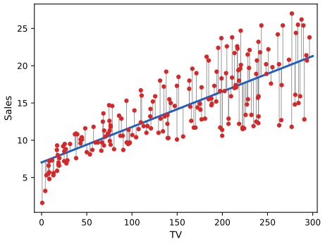
fig_3_1. Reproduces James et al. (2021), Figure 3.1. Download: PDF · SVG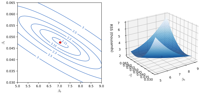
3.1.2 Assessing the Accuracy of the Coefficient Estimates
pp. 63–65 If the truth is (3.5), the population regression line is fixed, but the least-squares line changes from one data set to the next. Figure 3.3 shows this on simulated data from
\[ Y=2+3X+\epsilon. \tag{3.6} \]The analogy is the sample mean \(\hat\mu=\bar y\) as an estimate of a population mean \(\mu\): it is unbiased (on average over many data sets it equals \(\mu\)), and its typical error is measured by its standard error,
\[ \Var(\hat\mu)=\SE(\hat\mu)^2=\frac{\sigma^2}{n}, \tag{3.7} \]where \(\sigma\) is the standard deviation of each \(y_i\) and the observations are uncorrelated. The least-squares estimates are unbiased in the same sense, and their standard errors are
\[ \SE(\hat\beta_0)^2=\sigma^2\Big[\frac1n+\frac{\bar x^2}{\sum_{i=1}^n(x_i-\bar x)^2}\Big],\qquad \SE(\hat\beta_1)^2=\frac{\sigma^2}{\sum_{i=1}^n(x_i-\bar x)^2}, \tag{3.8} \]with \(\sigma^2=\Var(\epsilon)\), valid when the errors have a common variance and are uncorrelated. The slope is estimated more precisely when the \(x_i\) are spread out. In practice \(\sigma\) is unknown and is replaced by the residual standard error \(\RSE=\sqrt{\RSS/(n-2)}\).
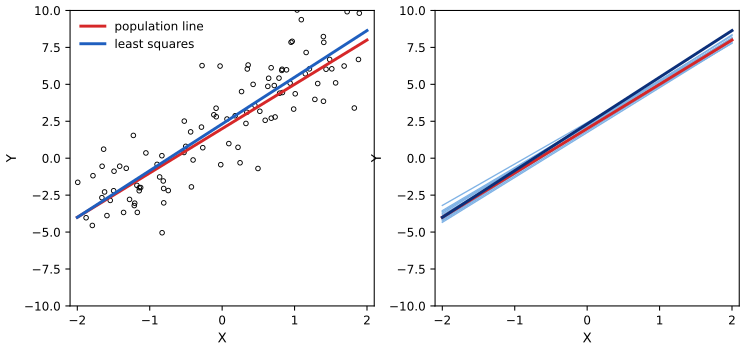
fig_3_3. Reproduces James et al. (2021), Figure 3.3. Download: PDF · SVGFilling the gap 3.2: unbiasedness, the standard errors (3.8) and why RSS is divided by \(n-2\) pp. 65–66
Both estimates are weighted sums of the \(y_i\) with known weights; their means and variances follow from the rules for sums of uncorrelated variables. The same computation shows that \(\E(\RSS)=(n-2)\sigma^2\), so \(\RSE^2\) is an unbiased estimate of \(\sigma^2\).
Derivation
Setting. The \(x_i\) are treated as fixed, \(y_i=\beta_0+\beta_1x_i+\epsilon_i\) with \(\E\epsilon_i=0\), \(\Var\epsilon_i=\sigma^2\) and \(\Cov(\epsilon_i,\epsilon_j)=0\) for \(i\ne j\).
The slope. Since \(\sum_i(x_i-\bar x)\bar y=0\), the slope is \(\hat\beta_1=\sum_ic_iy_i\) with weights \(c_i=(x_i-\bar x)/S_{xx}\). These weights satisfy \(\sum_ic_i=0\), \(\sum_ic_ix_i=\sum_ic_i(x_i-\bar x)=1\) and \(\sum_ic_i^2=1/S_{xx}\). Hence
\[ \E\hat\beta_1=\sum_ic_i(\beta_0+\beta_1x_i)=\beta_1,\qquad \Var\hat\beta_1=\sum_ic_i^2\,\sigma^2=\frac{\sigma^2}{S_{xx}}, \]using that the variance of a sum of uncorrelated terms is the sum of the variances. Equivalently \(\hat\beta_1-\beta_1=\sum_ic_i\epsilon_i\).
The intercept. \(\hat\beta_0=\bar y-\hat\beta_1\bar x=\sum_i(1/n-\bar xc_i)y_i\), so \(\E\hat\beta_0=\beta_0+\beta_1\bar x-\beta_1\bar x=\beta_0\) and
\[ \Var\hat\beta_0=\sigma^2\sum_i\Big(\frac1n-\bar xc_i\Big)^2=\sigma^2\Big[\frac1n-\frac{2\bar x}{n}\sum_ic_i+\bar x^2\sum_ic_i^2\Big]=\sigma^2\Big[\frac1n+\frac{\bar x^2}{S_{xx}}\Big]. \]The same bookkeeping gives \(\Cov(\hat\beta_0,\hat\beta_1)=-\bar x\,\sigma^2/S_{xx}\): when \(\bar x>0\) an overestimated slope comes with an underestimated intercept, the tilt of the ellipses in Figure 3.2. With all weights equal to \(1/n\) the same rule gives (3.7). If \(\bar x=0\), \(\hat\beta_0=\bar y\) and \(\SE(\hat\beta_0)=\SE(\hat\mu)\), as the book remarks.
Why \(n-2\). The residuals are \(e_i=(\epsilon_i-\bar\epsilon)-(x_i-\bar x)(\hat\beta_1-\beta_1)\). Squaring and summing, and using \(\sum_i(x_i-\bar x)(\epsilon_i-\bar\epsilon)=S_{xx}(\hat\beta_1-\beta_1)\),
\[ \RSS=\sum_i(\epsilon_i-\bar\epsilon)^2-S_{xx}(\hat\beta_1-\beta_1)^2,\qquad \E\RSS=(n-1)\sigma^2-S_{xx}\cdot\frac{\sigma^2}{S_{xx}}=(n-2)\sigma^2. \]So \(\E(\RSE^2)=\sigma^2\). Fitting two coefficients uses up two “degrees of freedom”: the residuals are forced to satisfy the two equations \(\sum e_i=0\) and \(\sum x_ie_i=0\), so they are a little smaller than the errors. ∎
A remark on wording. The book says the standard error is “the average amount” by which the estimate differs from the truth. Precisely, it is the root mean square difference, \(\sqrt{\E(\hat\beta_1-\beta_1)^2}\); for a normal estimate the average absolute difference is \(\sqrt{2/\pi}\approx0.80\) times the standard error.
pp. 66–68 A 95% confidence interval is a range computed from the data that contains the true parameter in 95% of repeated samples. For the slope it is approximately
\[ \hat\beta_1\pm2\cdot\SE(\hat\beta_1), \tag{3.9} \]that is, the interval
\[ \big[\hat\beta_1-2\cdot\SE(\hat\beta_1),\ \hat\beta_1+2\cdot\SE(\hat\beta_1)\big] \tag{3.10} \]contains \(\beta_1\) with probability about 0.95, and similarly
\[ \hat\beta_0\pm2\cdot\SE(\hat\beta_0). \tag{3.11} \]For the Advertising data the 95% intervals are \([6.130, 7.935]\) for \(\beta_0\) and \([0.042, 0.053]\) for \(\beta_1\). Standard errors also give hypothesis tests. The usual one compares
\[ H_0:\ \text{there is no relationship between } X \text{ and } Y \tag{3.12} \]with
\[ H_a:\ \text{there is some relationship between } X \text{ and } Y, \tag{3.13} \]that is \(H_0:\beta_1=0\) against \(H_a:\beta_1\ne0\), through the t-statistic
\[ t=\frac{\hat\beta_1-0}{\SE(\hat\beta_1)}, \tag{3.14} \]the number of standard errors by which \(\hat\beta_1\) is away from zero. If \(\beta_1=0\), \(t\) has a t-distribution with \(n-2\) degrees of freedom, and the p-value is the probability, computed under \(H_0\), of a value at least as large as \(|t|\). A small p-value says that an association this strong would be unlikely by chance alone.
| Coefficient | Std. error | t-statistic | p-value | |
|---|---|---|---|---|
| Intercept | 7.0326 | 0.4578 | 15.36 | < 0.0001 |
| TV | 0.0475 | 0.0027 | 17.67 | < 0.0001 |
Filling the gap 3.3: where the “2” comes from, the exact t-interval and the t-test pp. 66–68 and footnote 3
With normal errors, \((\hat\beta_1-\beta_1)/\SE(\hat\beta_1)\) has exactly a t-distribution with \(n-2\) degrees of freedom. The exact 95% interval replaces the 2 of (3.9) by the 97.5% point of that distribution, 1.972 for \(n=200\); this is what the book's printed intervals use.
Derivation
Three facts under \(\epsilon_i\sim N(0,\sigma^2)\) independent: (i) \(\hat\beta_1=\beta_1+\sum_ic_i\epsilon_i\) is a linear combination of normals, so \(\hat\beta_1\sim N(\beta_1,\sigma^2/S_{xx})\) (Filling the gap 3.2); (ii) \(\RSS/\sigma^2\) has a chi-squared distribution with \(n-2\) degrees of freedom; (iii) \(\RSS\) is independent of \(\hat\beta_1\). Facts (ii) and (iii) come from writing the residual vector as an orthogonal projection of the error vector; the full argument is in the graduate course (link below).
The pivot. By definition a \(t_{\nu}\) variable is \(Z/\sqrt{W/\nu}\) with \(Z\sim N(0,1)\) and \(W\sim\chi^2_\nu\) independent. Take \(Z=(\hat\beta_1-\beta_1)/(\sigma/\sqrt{S_{xx}})\) and \(W=\RSS/\sigma^2\), \(\nu=n-2\):
\[ T=\frac{Z}{\sqrt{W/(n-2)}}=\frac{\hat\beta_1-\beta_1}{\RSE/\sqrt{S_{xx}}}=\frac{\hat\beta_1-\beta_1}{\SE(\hat\beta_1)}\sim t_{n-2}. \]The unknown \(\sigma\) cancels: that is why the t-distribution, and not the normal, is the right reference when \(\sigma\) is estimated.
The interval. With \(q=t_{n-2}^{(0.975)}\), \(\Pr(-q\le T\le q)=0.95\); solving the two inequalities for \(\beta_1\) gives \(\Pr\big(\hat\beta_1-q\,\SE\le\beta_1\le\hat\beta_1+q\,\SE\big)=0.95\). The interval is random and \(\beta_1\) is fixed: “95%” is the proportion of samples whose interval covers the truth. For \(n=200\), \(q=1.972\): \(7.0326\pm1.972\times0.4578=[6.130,7.935]\) and \(0.0475\pm1.972\times0.0027=[0.042,0.053]\), the book's numbers. With the rounded factor 2 the intercept interval would be \([6.117,7.948]\).
The test. Under \(H_0:\beta_1=0\), \(t=\hat\beta_1/\SE(\hat\beta_1)\sim t_{n-2}\), and the two-sided p-value is \(2\Pr(T_{n-2}\ge|t|)\). Rejecting when \(p<0.05\) is the same as rejecting when the 95% interval excludes 0. For \(n=30\) (28 degrees of freedom) the cut-offs for 5% and 1% are \(|t|>2.05\) and \(|t|>2.76\), the “around 2 and 2.75” of p. 68. For TV, \(t=0.0475/0.0027=17.67\), and \(p\approx10^{-42}\).
Without normal errors the same statements hold approximately when \(n\) is large, by the central limit theorem applied to \(\sum_ic_i\epsilon_i\). ∎
Deeper: Statistical Learning: Theory and Methods, Result 3.4 and Filling the gap 3.1 there (the joint distribution of the estimates and of RSS, with proof of facts (ii) and (iii)), and Result 3.5 (the t and F tests).
See also (companion course): Statistical Methods for Modern Biology, Section 6.5 (the t-test, in R).
3.1.3 Assessing the Accuracy of the Model
pp. 68–71 Once \(H_0\) is rejected, we want to know how well the line fits. Even the true line cannot predict \(Y\) exactly because of \(\epsilon\). The residual standard error estimates the standard deviation of \(\epsilon\):
\[ \RSE=\sqrt{\frac{1}{n-2}\RSS}=\sqrt{\frac{1}{n-2}\sum_{i=1}^n(y_i-\hat y_i)^2}, \tag{3.15} \]with
\[ \RSS=\sum_{i=1}^n(y_i-\hat y_i)^2. \tag{3.16} \]For sales on TV, \(\RSE=3.26\): actual sales deviate from the line by about 3,260 units, which is 23% of the mean sales of 14,000 units. The RSE is in the units of \(Y\), so it is hard to judge in the abstract. The \(R^2\) statistic is a proportion instead,
\[ R^2=\frac{\TSS-\RSS}{\TSS}=1-\frac{\RSS}{\TSS}, \tag{3.17} \]where \(\TSS=\sum_i(y_i-\bar y)^2\) is the total sum of squares, the variability of \(Y\) before the regression. \(R^2\) is the fraction of that variability explained by \(X\). Here \(R^2=0.612\). What counts as a good \(R^2\) depends on the field: close to 1 in some physical experiments, well below 0.1 in much of biology, psychology or marketing. The correlation
\[ \Cor(X,Y)=\frac{\sum_{i=1}^n(x_i-\bar x)(y_i-\bar y)}{\sqrt{\sum_{i=1}^n(x_i-\bar x)^2}\sqrt{\sum_{i=1}^n(y_i-\bar y)^2}} \tag{3.18} \]also measures linear association, and in simple regression \(R^2=r^2\) with \(r=\Cor(X,Y)\): for TV, \(r=0.782\) and \(r^2=0.612\).
| Quantity | Value |
|---|---|
| Residual standard error | 3.26 |
| \(R^2\) | 0.612 |
| F-statistic | 312.1 |
Filling the gap 3.4: the decomposition \(\TSS=\RSS+\ESS\), and \(R^2=r^2\) p. 71, “it can be shown that in the simple linear regression setting, \(R^2=r^2\)” (also Exercise 7)
The total variability splits exactly into an unexplained part (RSS) and an explained part \(\ESS=\sum_i(\hat y_i-\bar y)^2\); this is why \(0\le R^2\le1\). In simple regression the explained part is \(S_{xy}^2/S_{xx}\), and \(R^2\) collapses to the squared correlation.
Derivation
The decomposition. Write \(y_i-\bar y=e_i+(\hat y_i-\bar y)\). Squaring and summing,
\[ \TSS=\RSS+\ESS+2\sum_ie_i(\hat y_i-\bar y). \]Since \(\hat y_i-\bar y=\hat\beta_1(x_i-\bar x)\) (the line passes through \((\bar x,\bar y)\)), the cross term is \(2\hat\beta_1\sum_ie_i(x_i-\bar x)=0\) by the normal equations of Filling the gap 3.1. Hence \(\TSS=\RSS+\ESS\), and \(R^2=\ESS/\TSS\in[0,1]\). (This needs the intercept: without it \(\sum e_i\) need not vanish, and software then defines \(R^2\) with \(\sum y_i^2\) in place of TSS.)
\(R^2=r^2\). \[ \ESS=\hat\beta_1^2S_{xx}=(S_{xy}/S_{xx})^2S_{xx}=S_{xy}^2/S_{xx}. \] Therefore
\[ R^2=\frac{\ESS}{\TSS}=\frac{S_{xy}^2}{S_{xx}S_{yy}}=\Big(\frac{S_{xy}}{\sqrt{S_{xx}}\sqrt{S_{yy}}}\Big)^2=r^2. \]With the simplification of Exercise 7 (\(\bar x=\bar y=0\)) the sums become \(\sum x_iy_i\), \(\sum x_i^2\), \(\sum y_i^2\) and the computation is the same.
The F-statistic of Table 3.2. In simple regression \[ F=\ESS/(\RSS/(n-2))=(n-2)R^2/(1-R^2), \] which also equals \(t^2\) for the slope: \(198\times0.612/0.388=312.1=17.67^2\). ∎
Confirmed numerically for TV, radio and newspaper.
3.2 Multiple Linear Regression
pp. 71–72 With three media we could run three simple regressions (Tables 3.1 and 3.3). That is unsatisfactory: there is no single prediction from three budgets, and each simple regression ignores the other two media, which misleads when the budgets are correlated across markets.
| Coefficient | Std. error | t-statistic | p-value | |
|---|---|---|---|---|
| Intercept | 9.312 | 0.563 | 16.54 | < 0.0001 |
| radio | 0.203 | 0.020 | 9.92 | < 0.0001 |
| Intercept | 12.351 | 0.621 | 19.88 | < 0.0001 |
| newspaper | 0.055 | 0.017 | 3.30 | 0.00115 |
Definition 3.2 (multiple linear regression) p. 72, (3.19)–(3.20)
With \(p\) predictors the model gives each predictor its own slope,
\[ Y=\beta_0+\beta_1X_1+\beta_2X_2+\dots+\beta_pX_p+\epsilon. \tag{3.19} \]\(\beta_j\) is the average change in \(Y\) for a one-unit increase in \(X_j\) with all other predictors held fixed. For the Advertising data,
\[ \texttt{sales}=\beta_0+\beta_1\times\texttt{TV}+\beta_2\times\texttt{radio}+\beta_3\times\texttt{newspaper}+\epsilon. \tag{3.20} \]3.2.1 Estimating the Regression Coefficients
pp. 72–75 Given estimates, predictions are
\[ \hat y=\hat\beta_0+\hat\beta_1x_1+\hat\beta_2x_2+\dots+\hat\beta_px_p, \tag{3.21} \]and least squares again minimises the residual sum of squares
\[ \RSS=\sum_{i=1}^n(y_i-\hat y_i)^2=\sum_{i=1}^n(y_i-\hat\beta_0-\hat\beta_1x_{i1}-\hat\beta_2x_{i2}-\dots-\hat\beta_px_{ip})^2. \tag{3.22} \]The book does not write the solution down because it needs matrices; it is short, and Filling the gap 3.5 gives it. With two predictors the fit is a plane (Figure 3.4).
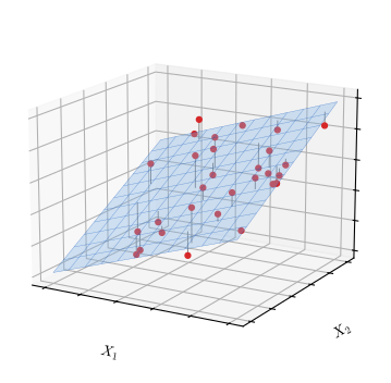
fig_3_4. Reproduces James et al. (2021), Figure 3.4. Download: PDF · SVG| Coefficient | Std. error | t-statistic | p-value | |
|---|---|---|---|---|
| Intercept | 2.939 | 0.3119 | 9.42 | < 0.0001 |
| TV | 0.046 | 0.0014 | 32.81 | < 0.0001 |
| radio | 0.189 | 0.0086 | 21.89 | < 0.0001 |
| newspaper | −0.001 | 0.0059 | −0.18 | 0.8599 |
TV and radio have nearly the same slopes as in their simple regressions, but newspaper's slope drops from 0.055 (clearly non-zero) to \(-0.001\) (p = 0.86). There is no contradiction. The correlation matrix (Table 3.5) shows that newspaper and radio budgets are correlated (0.35): markets that spend on newspapers tend to spend on radio, and radio sells. Alone, newspaper gets the credit for radio. The book's illustration: ice-cream sales “predict” shark attacks until temperature is added to the model.
| TV | radio | newspaper | sales | |
|---|---|---|---|---|
| TV | 1.0000 | 0.0548 | 0.0567 | 0.7822 |
| radio | 1.0000 | 0.3541 | 0.5762 | |
| newspaper | 1.0000 | 0.2283 | ||
| sales | 1.0000 |
Filling the gap 3.5: the multiple-regression estimates, their standard errors, and what “holding the others fixed” means p. 73, “most easily represented using matrix algebra. For this reason, we do not provide them here”
In matrix form \(\hb=(\bX^\T\bX)^{-1}\bX^\T\by\) and \(\Var(\hb)=\sigma^2(\bX^\T\bX)^{-1}\). Each coefficient is also a simple regression: \(\hat\beta_j\) is the slope of \(y\) on the part of \(x_j\) that the other predictors cannot explain. That is what holding the others fixed means, and it explains newspaper exactly.
Derivation
Matrix form. Stack the responses in \(\by\) (length \(n\)) and the rows \((1,x_{i1},\dots,x_{ip})\) in \(\bX\) (\(n\times(p+1)\)). Then the fitted values are \(\bX\bb\) and \(\RSS(\bb)=(\by-\bX\bb)^\T(\by-\bX\bb)\). Its gradient is \(-2\bX^\T(\by-\bX\bb)\); setting it to zero gives the normal equations \(\bX^\T\bX\hb=\bX^\T\by\), and if the columns of \(\bX\) are linearly independent,
\[ \hb=(\bX^\T\bX)^{-1}\bX^\T\by. \]It is the minimum by the same argument as in Filling the gap 3.1: \(\RSS(\hb+\bd)=\RSS(\hb)+\|\bX\bd\|^2\). With one predictor, \(\bX^\T\bX=\begin{pmatrix}n&\sum x_i\\\sum x_i&\sum x_i^2\end{pmatrix}\) and the formula reduces to (3.4).
Mean and variance. \[ \hb=(\bX^\T\bX)^{-1}\bX^\T(\bX\bb+\boldsymbol\epsilon)=\bb+(\bX^\T\bX)^{-1}\bX^\T\boldsymbol\epsilon, \] so \(\E\hb=\bb\) and, with \(\Var(\boldsymbol\epsilon)=\sigma^2\bI\), \[ \Var(\hb)=(\bX^\T\bX)^{-1}\bX^\T(\sigma^2\bI)\bX(\bX^\T\bX)^{-1}=\sigma^2(\bX^\T\bX)^{-1}. \] The standard error of \(\hat\beta_j\) is \(\RSE\) times the square root of the \(j\)th diagonal entry of \((\bX^\T\bX)^{-1}\), with \(\RSE^2=\RSS/(n-p-1)\) unbiased for \(\sigma^2\) (one degree of freedom per coefficient, as in Filling the gap 3.2).
Each coefficient as a simple regression. Regress \(x_j\) on the other predictors (with an intercept) and call the residuals \(r_{1j},\dots,r_{nj}\): the part of \(x_j\) not explained by the others. Then
\[ \hat\beta_j=\frac{\sum_ir_{ij}y_i}{\sum_ir_{ij}^2},\qquad \Var(\hat\beta_j)=\frac{\sigma^2}{\sum_ir_{ij}^2}. \]Proof. Write the fit as \(\hat\by=\bX_{-j}\boldsymbol\gamma+\hat\beta_j\bx_j\) and \(\bx_j=\br_j+\bX_{-j}\bd\), where \(\bX_{-j}\) holds the other columns. The residual vector \(\by-\hat\by\) is orthogonal to every column of \(\bX\) (normal equations), hence to \(\br_j\), and \(\br_j\) is orthogonal to the columns of \(\bX_{-j}\). So \(\br_j^\T\by=\br_j^\T\hat\by=\hat\beta_j\br_j^\T\bx_j=\hat\beta_j\br_j^\T\br_j\). The variance follows as in Filling the gap 3.2, since \(\br_j\) does not depend on \(\by\). ∎
Newspaper. Regressing newspaper on TV and radio leaves residuals that carry 87% of its variance, and the slope of sales on those residuals is \(-0.0010\): exactly the coefficient of Table 3.4. The simple slope of Table 3.3 splits exactly as
\[ 0.0547=\underbrace{-0.0010}_{\text{newspaper}}+\underbrace{0.1885\times0.241}_{\text{radio}}+\underbrace{0.0458\times0.223}_{\text{TV}}, \]where 0.241 and 0.223 are the slopes of radio and of TV on newspaper. Almost all of newspaper's simple association is radio's effect, carried by the correlation of the budgets. (This “omitted variable” identity holds exactly for least-squares fits on the same data.)
Confirmed numerically on the Advertising data.
Deeper: Statistical Learning: Theory and Methods, Section 3.2 (least squares in matrix form, the hat matrix and the geometry of projections) and Section 3.2.3 (multiple regression from simple regressions, the Gram–Schmidt view of the adjusted predictors above); Section 3.2.2 (the Gauss–Markov theorem: least squares has the smallest variance among unbiased linear estimators).
See also (companion courses): Bayesian and Probabilistic Machine Learning, Section 3.1.1 (least squares as the maximum-likelihood estimate under normal errors) and Section 3.1.2 (its geometry).
3.2.2 Some Important Questions
p. 75 Four questions guide a multiple regression: (1) is at least one predictor useful? (2) do all predictors help, or only some? (3) how well does the model fit? (4) what should we predict, and how accurately?
One: is there a relationship between the response and the predictors?
pp. 75–78 We test \(H_0:\beta_1=\beta_2=\dots=\beta_p=0\) against \(H_a\): at least one \(\beta_j\) is non-zero, with the F-statistic
\[ F=\frac{(\TSS-\RSS)/p}{\RSS/(n-p-1)}. \tag{3.23} \]If the model is right, \(\E\{\RSS/(n-p-1)\}=\sigma^2\), and under \(H_0\) also \(\E\{(\TSS-\RSS)/p\}=\sigma^2\), so \(F\) is near 1; under \(H_a\) the numerator is larger on average. With normal errors and \(H_0\) true, \(F\) follows an F-distribution with \(p\) and \(n-p-1\) degrees of freedom. For the Advertising data \(F=570\) (Table 3.6), and the p-value is about \(10^{-96}\).
| Quantity | Value |
|---|---|
| Residual standard error | 1.69 |
| \(R^2\) | 0.897 |
| F-statistic | 570 |
To test that a particular set of \(q\) coefficients is zero, say \(H_0:\beta_{p-q+1}=\dots=\beta_p=0\), fit the model without those \(q\) predictors, call its residual sum of squares \(\RSS_0\), and use
\[ F=\frac{(\RSS_0-\RSS)/q}{\RSS/(n-p-1)}. \tag{3.24} \]With \(q=1\) this is exactly the square of the t-statistic of the dropped variable (footnote 7 of the book): the t-tests of Table 3.4 measure the effect of adding each variable last. Why then look at the overall F at all? Because with many predictors some individual p-values will be small by chance. With \(p=100\) predictors none of which matters, about five p-values below 0.05 are expected, and at least one is almost certain; the F-test, in contrast, has a 5% false alarm rate whatever \(p\) and \(n\). The F-test needs \(p<n\); when \(p>n\) least squares cannot even be fitted (Chapter 6).
Filling the gap 3.6: the F-statistic (3.23) and (3.24), and why separate t-tests are not enough p. 76, “one can show that”; p. 77, footnote 7
Both expectations quoted on p. 76 follow from one formula for the expected value of a squared projection. With normal errors the two sums of squares are independent chi-squared variables, so \(F\) has an F-distribution; with \(q=1\), \(F=t^2\). Separate tests at level 5% on 100 useless predictors raise at least one false alarm with probability close to \(1-0.95^{100}=0.994\).
Derivation
A projection identity. Let \(\bH=\bX(\bX^\T\bX)^{-1}\bX^\T\), the matrix that maps \(\by\) to \(\hat\by\). It is symmetric with \(\bH^2=\bH\) (projecting twice changes nothing) and trace \(p+1\). For any such projection \(\bP\) of rank \(k\) and \(\by=\boldsymbol\mu+\boldsymbol\epsilon\) with \(\Var\boldsymbol\epsilon=\sigma^2\bI\),
\[ \E\|\bP\by\|^2=\|\bP\boldsymbol\mu\|^2+\E\,\boldsymbol\epsilon^\T\bP\boldsymbol\epsilon=\|\bP\boldsymbol\mu\|^2+\sigma^2\tr\bP=\|\bP\boldsymbol\mu\|^2+k\sigma^2. \]The denominator. \(\RSS=\|(\bI-\bH)\by\|^2\) with \(\bI-\bH\) of rank \(n-p-1\) and \((\bI-\bH)\bX\bb=\mathbf0\), so \(\E\RSS=(n-p-1)\sigma^2\).
The numerator. With \(\bJ=\bone\bone^\T/n\) (which replaces each \(y_i\) by \(\bar y\)), \(\TSS-\RSS=\ESS=\|(\bH-\bJ)\by\|^2\), and \(\bH-\bJ\) is a projection of rank \(p\) (the column of ones lies in the column space of \(\bX\)). So
\[ \E(\TSS-\RSS)=p\,\sigma^2+\sum_{i=1}^n\big(f(x_i)-\bar f\big)^2,\qquad f(x_i)=\beta_0+\textstyle\sum_j\beta_jx_{ij}. \]Under \(H_0\) the regression function is constant and the second term is zero, giving \(\E\{(\TSS-\RSS)/p\}=\sigma^2\); under \(H_a\) the second term is positive (unless the predictors are constant), so the numerator of \(F\) tends to exceed \(\sigma^2\).
The distribution. With normal errors, \(\ESS/\sigma^2\sim\chi^2_p\) under \(H_0\) and \(\RSS/\sigma^2\sim\chi^2_{n-p-1}\), and they are independent because \(\bH-\bJ\) and \(\bI-\bH\) project onto orthogonal subspaces. A ratio of independent chi-squared variables, each divided by its degrees of freedom, is by definition F-distributed. The same argument with \(\bH-\bH_0\) (\(\bH_0\) the hat matrix of the smaller model, rank difference \(q\)) gives (3.24).
\(F=t^2\) when \(q=1\). By Filling the gap 3.5, adding \(x_j\) last adds the direction \(\br_j\) to the column space, so \(\RSS_0-\RSS=(\br_j^\T\by)^2/\|\br_j\|^2=\hat\beta_j^2\|\br_j\|^2\), while \(\SE(\hat\beta_j)^2=\RSE^2/\|\br_j\|^2\). Hence \[ F=(\RSS_0-\RSS)/\RSE^2=\hat\beta_j^2/\SE(\hat\beta_j)^2=t_j^2. \] For newspaper: \((-0.177)^2=0.031\), and (3.24) for dropping newspaper gives the same 0.031.
Many t-tests. If 100 independent tests are each run at level 0.05 with every null true, \[ \Pr(\text{at least one } p<0.05)=1-0.95^{100}=0.994, \] and the expected number of false alarms is 5. The t-statistics of one regression are not exactly independent, but the conclusion does not change. In 300 simulated data sets with \(n=500\) and 100 useless predictors, 295 had at least one individual p-value below 0.05, while the F-test rejected in 20 (close to the nominal 15). ∎
Confirmed numerically: the two expectations and the F-distribution under \(H_0\) by simulation, and \(F=t^2\) on the Advertising data.
Deeper: Statistical Learning: Theory and Methods, Result 3.5 and Filling the gap 3.2 there (the exact t and F distributions, and the F-test for groups of coefficients).
See also (companion course): Statistical Methods for Modern Biology, Section 6.7 (multiple testing) and Section 6.8.1 (the Bonferroni correction); Chapter 13 of the book returns to the subject.
Two: deciding on important variables
pp. 78–79 Choosing the predictors that are truly associated with the response is variable selection, the subject of Chapter 6. Models can be compared with Mallows' \(C_p\), the Akaike information criterion (AIC), the Bayesian information criterion (BIC) and adjusted \(R^2\), or by plotting residuals. Trying all \(2^p\) subsets is out of reach even for moderate \(p\) (\(2^{30}=1{,}073{,}741{,}824\)), so three greedy searches are classical:
Algorithm 3.1 (classical variable selection) p. 79
- Forward selection. Start from the null model (intercept only). Fit the \(p\) simple regressions and add the variable with the smallest RSS; then add the variable that gives the smallest RSS for the two-variable model; continue until a stopping rule is met.
- Backward selection. Start from all variables; remove the one with the largest p-value, refit, and repeat until all remaining p-values are below a threshold. Impossible when \(p>n\).
- Mixed selection. Proceed forwards, but after each addition remove any variable whose p-value has risen above a threshold; stop when every variable in the model has a small p-value and every variable outside would have a large one if added.
Forward selection is greedy and can keep a variable that later becomes redundant; mixed selection corrects this.
Deeper: Statistical Learning: Theory and Methods, Section 3.3 (best-subset, forward- and backward-stepwise and forward-stagewise selection, with the leaps-and-bounds algorithm and the prostate cancer example).
Three: model fit
pp. 79–81 RSE and \(R^2\) are read as in simple regression. In multiple regression \(R^2=\Cor(Y,\hat Y)^2\), and the least-squares fit maximises this correlation among all linear functions of the predictors. \(R^2\) can only grow when a variable is added: with TV, radio and newspaper \(R^2=0.8972\), with TV and radio alone 0.89719. That tiny increase, together with the large p-value, says newspaper can be dropped. The general RSE is
\[ \RSE=\sqrt{\frac{1}{n-p-1}\RSS}, \tag{3.25} \]which reduces to (3.15) when \(p=1\). It can increase when a variable is added (1.681 for TV and radio, 1.686 with newspaper too), because the small drop in RSS does not pay for the lost degree of freedom.
Filling the gap 3.7: \(R^2=\Cor(Y,\hat Y)^2\), least squares maximises the correlation, and \(R^2\) never falls when a variable is added p. 79, “it turns out that it equals \(\Cor(Y,\hat Y)^2\) … it maximizes this correlation”
The fitted values have the same mean as \(y\) and are uncorrelated with the residuals; both facts give the identity, and an inequality of Cauchy–Schwarz type gives the maximum.
Derivation
The identity. The normal equations say \(\sum_ie_i=0\) and \(\sum_ie_ix_{ij}=0\) for each \(j\); hence the mean of the \(\hat y_i\) is \(\bar y\) and \(\sum_ie_i(\hat y_i-\bar y)=0\). So \(\sum_i(y_i-\bar y)(\hat y_i-\bar y)=\sum_i(\hat y_i-\bar y)^2=\ESS\), and
\[ \Cor(y,\hat y)^2=\frac{\ESS^2}{\TSS\cdot\ESS}=\frac{\ESS}{\TSS}=R^2, \]using \(\TSS=\RSS+\ESS\) exactly as in Filling the gap 3.4.
The maximum. Let \(z_i=b_0+\sum_jb_jx_{ij}\) be any linear function of the predictors. Its deviations \(z_i-\bar z\) are again a linear combination of the predictor columns and the ones column, so \(\sum_ie_i(z_i-\bar z)=0\), and therefore \(\sum_i(y_i-\bar y)(z_i-\bar z)=\sum_i(\hat y_i-\bar y)(z_i-\bar z)\). By the Cauchy–Schwarz inequality this is at most \(\sqrt{\ESS}\sqrt{\sum_i(z_i-\bar z)^2}\), so
\[ \Cor(y,z)\le\frac{\sqrt{\ESS}}{\sqrt{\TSS}}=\sqrt{R^2}, \]with equality when \(z\) is an increasing linear function of \(\hat y\).
Adding a variable. The larger model's RSS is a minimum over a larger set of coefficient vectors (the smaller model is the special case with the new coefficient equal to zero), so it cannot be larger. TSS does not change, so \(R^2\) cannot fall. The adjusted \(R^2\), \(1-\frac{\RSS/(n-p-1)}{\TSS/(n-1)}=1-\RSE^2/s_y^2\), moves in the opposite direction to the RSE and can fall: 0.8962 for TV and radio, 0.8956 with newspaper. ∎
Confirmed numerically: on the Advertising data, \(\Cor(y,\hat y)^2\) equals \(R^2\), and none of 500 random perturbations of the coefficients gives a larger correlation.
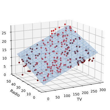
fig_3_5. Reproduces James et al. (2021), Figure 3.5. Download: PDF · SVGFour: predictions
pp. 81–82 A prediction from (3.21) carries three kinds of uncertainty: the coefficients are estimates (reducible error, measured by a confidence interval for \(f(X)\)); the linear form is only an approximation (model bias, ignored here); and even a perfectly known \(f\) cannot predict the error \(\epsilon\) of a new observation (irreducible error). A prediction interval for a new \(Y\) includes the last source and is always wider. With $100,000 on TV and $20,000 on radio (model with TV and radio), the 95% confidence interval for the mean sales over many such cities is [10,985, 11,528] units and the 95% prediction interval for the sales of one city is [7,930, 14,580] (14,583 unrounded); both are centred at 11,256.
Filling the gap 3.8: the formulas for the confidence and the prediction interval pp. 81–82
At a new input \(x_0\) (with a leading 1), \(\hat f(x_0)=x_0^\T\hb\) has variance \(\sigma^2x_0^\T(\bX^\T\bX)^{-1}x_0\). The prediction error \(Y_0-\hat f(x_0)\) adds the variance \(\sigma^2\) of the new error. Hence
\[ \text{CI: }\ \hat f(x_0)\pm t_{n-p-1}^{(0.975)}\,\RSE\sqrt{x_0^\T(\bX^\T\bX)^{-1}x_0},\qquad \text{PI: }\ \hat f(x_0)\pm t_{n-p-1}^{(0.975)}\,\RSE\sqrt{1+x_0^\T(\bX^\T\bX)^{-1}x_0}. \]Derivation
Confidence interval. \(\hat f(x_0)=x_0^\T\hb\) is a fixed linear combination of the coefficients, so by Filling the gap 3.5 its mean is \(f(x_0)\) and its variance \(x_0^\T\Var(\hb)x_0=\sigma^2x_0^\T(\bX^\T\bX)^{-1}x_0\). In simple regression this is
\[ \Var\hat f(x_0)=\sigma^2\Big[\frac1n+\frac{(x_0-\bar x)^2}{S_{xx}}\Big], \](combine \(\Var\hat\beta_0\), \(\Var\hat\beta_1\) and \(\Cov(\hat\beta_0,\hat\beta_1)\) of Filling the gap 3.2): smallest at \(x_0=\bar x\), growing quadratically away from it. Replacing \(\sigma\) by RSE and the normal quantile by the t quantile gives the interval, exactly as in Filling the gap 3.3.
Prediction interval. A new response is \(Y_0=f(x_0)+\epsilon_0\) with \(\epsilon_0\) independent of the training data. Then \(Y_0-\hat f(x_0)=\epsilon_0-(\hat f(x_0)-f(x_0))\) has mean 0 and variance \(\sigma^2+\Var\hat f(x_0)\). Under normal errors it is normal and independent of RSS, so the same t argument applies with \(\sqrt{1+x_0^\T(\bX^\T\bX)^{-1}x_0}\).
What this means. As \(n\) grows the confidence interval shrinks to a point (the term \(x_0^\T(\bX^\T\bX)^{-1}x_0\) is of order \(1/n\)), while the prediction interval tends to \(f(x_0)\pm1.96\sigma\): no amount of data removes the irreducible error. For the TV and radio model at \((100,20)\): \(\hat f=11.256\), \(\RSE\sqrt{x_0^\T(\bX^\T\bX)^{-1}x_0}=0.138\) and \(\RSE\sqrt{1+\dots}=1.687\), so the intervals are \(11.256\pm1.972\times0.138=[10.985,11.528]\) and \(11.256\pm1.972\times1.687=[7.930,14.583]\). ∎
Confirmed numerically against the book's intervals and against the interval functions of R (predict) and Python (get_prediction) in the lab.
Deeper: Statistical Learning: Theory and Methods, Filling the gap 3.3 (pointwise intervals for \(f(x_0)\) and a band that covers the whole regression function simultaneously).
3.3 Other Considerations in the Regression Model
3.3.1 Qualitative Predictors
pp. 83–87 The Credit data record, for 400 credit-card holders, the average balance (the response) and quantitative predictors (age, number of cards, years of education, income in thousands of dollars, credit limit, credit rating; Figure 3.6), and four qualitative ones: own (house ownership), student, status (married or not) and region (East, South, West).
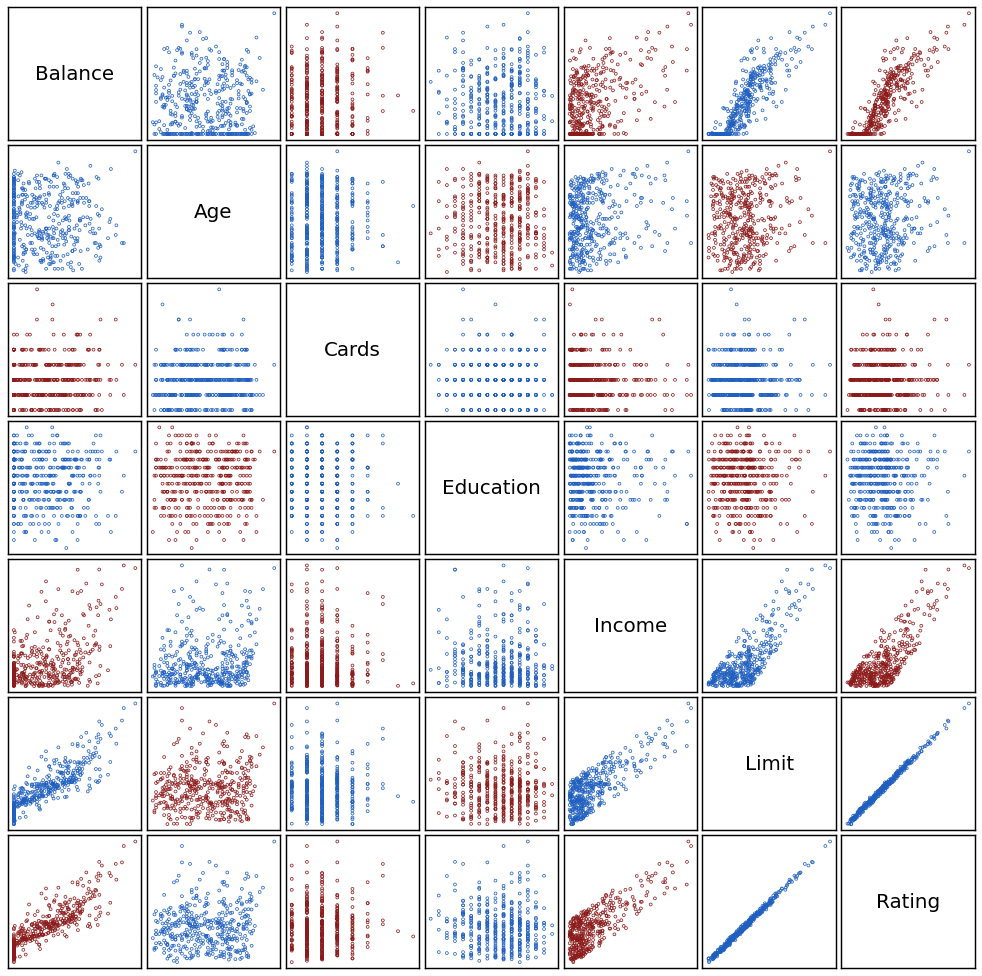
fig_3_6. Reproduces James et al. (2021), Figure 3.6. Download: PDF · SVG
Definition 3.3 (dummy variables) pp. 83–86, (3.26)–(3.30)
A qualitative predictor (a factor) with two levels enters through one indicator or dummy variable; in machine learning this is called one-hot encoding. For house ownership,
\[ x_i=\begin{cases}1&\text{if the } i\text{th person owns a house}\\0&\text{if the } i\text{th person does not own a house,}\end{cases} \tag{3.26} \] \[ y_i=\beta_0+\beta_1x_i+\epsilon_i=\begin{cases}\beta_0+\beta_1+\epsilon_i&\text{if the } i\text{th person owns a house}\\\beta_0+\epsilon_i&\text{if the } i\text{th person does not.}\end{cases} \tag{3.27} \]A factor with \(k\) levels needs \(k-1\) dummies; the level without one is the baseline. For region with baseline East,
\[ x_{i1}=\begin{cases}1&\text{if from the South}\\0&\text{otherwise,}\end{cases} \tag{3.28} \] \[ x_{i2}=\begin{cases}1&\text{if from the West}\\0&\text{otherwise,}\end{cases} \tag{3.29} \] \[ y_i=\beta_0+\beta_1x_{i1}+\beta_2x_{i2}+\epsilon_i=\begin{cases}\beta_0+\beta_1+\epsilon_i&\text{South}\\\beta_0+\beta_2+\epsilon_i&\text{West}\\\beta_0+\epsilon_i&\text{East.}\end{cases} \tag{3.30} \]Owners carry on average $19.73 more debt than non-owners ($529.53 against $509.80), but with p = 0.669 there is no evidence of a real difference (Table 3.7). Coding owners as 1 and non-owners as \(-1\) instead gives \(\hat\beta_0=519.67\), halfway between the two means, and \(\hat\beta_1=9.87\), half the difference; the predictions do not change.
| Coefficient | Std. error | t-statistic | p-value | |
|---|---|---|---|---|
| Intercept | 509.80 | 33.13 | 15.389 | < 0.0001 |
| own[Yes] | 19.73 | 46.05 | 0.429 | 0.6690 |
| Coefficient | Std. error | t-statistic | p-value | |
|---|---|---|---|---|
| Intercept | 531.00 | 46.32 | 11.464 | < 0.0001 |
| region[South] | −12.50 | 56.68 | −0.221 | 0.8260 |
| region[West] | −18.69 | 65.02 | −0.287 | 0.7740 |
The estimated mean balance is $531.00 in the East; people in the South carry $12.50 less, and in the West $18.69 less. Neither difference is significant, and the F-test of \(H_0:\beta_1=\beta_2=0\), which does not depend on the coding, has p = 0.96: no evidence that balance depends on region. Dummy variables mix freely with quantitative predictors. Other codings (contrasts) give the same fit with differently interpreted coefficients.
Filling the gap 3.9: why dummy coefficients are group means, and why the choice of baseline does not matter pp. 84–86
A regression on an intercept and the \(k-1\) dummies of one factor fits each group by its own sample mean. Any other coding spans the same set of fitted vectors, so it gives the same predictions, the same RSS and the same F-test; only the meaning of the individual coefficients changes.
Derivation
Group means. With an intercept and dummies for levels 2 to \(k\), the fitted value for anyone in level \(\ell\) is \(\beta_0\) (level 1) or \(\beta_0+\beta_\ell\). So the model allows any value \(m_\ell\) per group, and RSS \(=\sum_\ell\sum_{i\in\ell}(y_i-m_\ell)^2\) is minimised group by group by the sample mean \(\bar y_\ell\) (the sum of squared deviations from a constant is smallest at the mean). Hence \(\hat\beta_0=\bar y_1\) and \(\hat\beta_\ell=\bar y_\ell-\bar y_1\). For region: \(\bar y_{\text{East}}=531.00\), \(\bar y_{\text{South}}=518.50\), \(\bar y_{\text{West}}=512.31\), giving \(-12.50\) for South and \(-18.69\) for West.
Changing the coding. Any coding that can represent every set of group means (another baseline, the \(\pm1\) coding, sum-to-zero contrasts) is a reparametrisation of the same \(k\) group means: the columns of the new model matrix span the same space as the old. Least squares projects \(\by\) onto that space, so the fitted values and RSS are the same. The F-statistic for “all group means equal” compares this RSS with the RSS of the intercept-only model, so it is the same too, while the t-tests of individual coefficients answer different questions under different codings. With the \(\pm1\) coding of own: \(\beta_0+\beta_1=\bar y_{\text{own}}\) and \(\beta_0-\beta_1=\bar y_{\text{not}}\), so \(\hat\beta_0=(529.54+509.80)/2=519.67\) and \(\hat\beta_1=9.87\). (The book's 519.665 and 9.865 halve the rounded means.)
Why \(k-1\) dummies. With an intercept and all \(k\) dummies, the dummies add up to the column of ones: the columns are linearly dependent, \(\bX^\T\bX\) is singular, and the coefficients are not identifiable (the “dummy variable trap”). ∎
See also (companion course): Statistical Methods for Modern Biology, Section 8.7 (multi-factor designs, model matrices and the analysis of variance in R).
3.3.2 Extensions of the Linear Model
pp. 87–92 The standard model is additive (the effect of \(X_j\) does not depend on the other predictors) and linear (a one-unit change in \(X_j\) has the same effect whatever the value of \(X_j\)). Both assumptions can be relaxed while staying inside linear regression.
Removing the additive assumption
Figure 3.5 suggested that TV and radio reinforce each other. Starting from \(Y=\beta_0+\beta_1X_1+\beta_2X_2+\epsilon\), add an interaction term, the product \(X_1X_2\):
\[ Y=\beta_0+\beta_1X_1+\beta_2X_2+\beta_3X_1X_2+\epsilon. \tag{3.31} \] \[ Y=\beta_0+(\beta_1+\beta_3X_2)X_1+\beta_2X_2+\epsilon=\beta_0+\tilde\beta_1X_1+\beta_2X_2+\epsilon, \tag{3.32} \]with \(\tilde\beta_1=\beta_1+\beta_3X_2\): the slope of \(X_1\) now depends on \(X_2\). (The book's example: units produced \[ \approx1.2+3.4\times\text{lines}+0.22\times\text{workers}+1.4\times(\text{lines}\times\text{workers}), \] so one more production line adds \(3.4+1.4\times\text{workers}\) units.) For the Advertising data,
\[ \texttt{sales}=\beta_0+\beta_1\times\texttt{TV}+\beta_2\times\texttt{radio}+\beta_3\times(\texttt{radio}\times\texttt{TV})+\epsilon=\beta_0+(\beta_1+\beta_3\times\texttt{radio})\times\texttt{TV}+\beta_2\times\texttt{radio}+\epsilon. \tag{3.33} \]| Coefficient | Std. error | t-statistic | p-value | |
|---|---|---|---|---|
| Intercept | 6.7502 | 0.248 | 27.23 | < 0.0001 |
| TV | 0.0191 | 0.002 | 12.70 | < 0.0001 |
| radio | 0.0289 | 0.009 | 3.24 | 0.0014 |
| TV×radio | 0.0011 | 0.000 | 20.73 | < 0.0001 |
The interaction is overwhelming (t = 20.7), and \(R^2\) rises from 89.7% to 96.8%: the interaction explains \((96.8-89.7)/(100-89.7)=69\%\) of the variability the additive model left over. An extra $1,000 of TV goes with \[ (\hat\beta_1+\hat\beta_3\times\texttt{radio})\times1000=19+1.1\times\texttt{radio} \] more units, and an extra $1,000 of radio with \(29+1.1\times\texttt{TV}\) more units.
The hierarchical principle: if an interaction is in the model, keep both main effects, even if their p-values are large. The coefficients of the main effects alone are then of little interest, and leaving them out changes the meaning of the interaction (Filling the gap 3.10).
A qualitative-by-quantitative interaction is especially easy to read. For balance on income and student status, without an interaction,
\[ \texttt{balance}_i\approx\beta_0+\beta_1\times\texttt{income}_i+\begin{cases}\beta_2&\text{student}\\0&\text{not}\end{cases}=\beta_1\times\texttt{income}_i+\begin{cases}\beta_0+\beta_2&\text{student}\\\beta_0&\text{not,}\end{cases} \tag{3.34} \]two parallel lines; with the product of income and the student dummy,
\[ \texttt{balance}_i\approx\beta_0+\beta_1\times\texttt{income}_i+\begin{cases}\beta_2+\beta_3\times\texttt{income}_i&\text{student}\\0&\text{not}\end{cases}=\begin{cases}(\beta_0+\beta_2)+(\beta_1+\beta_3)\times\texttt{income}_i&\text{student}\\\beta_0+\beta_1\times\texttt{income}_i&\text{not,}\end{cases} \tag{3.35} \]two lines with their own intercepts and slopes (Figure 3.7).
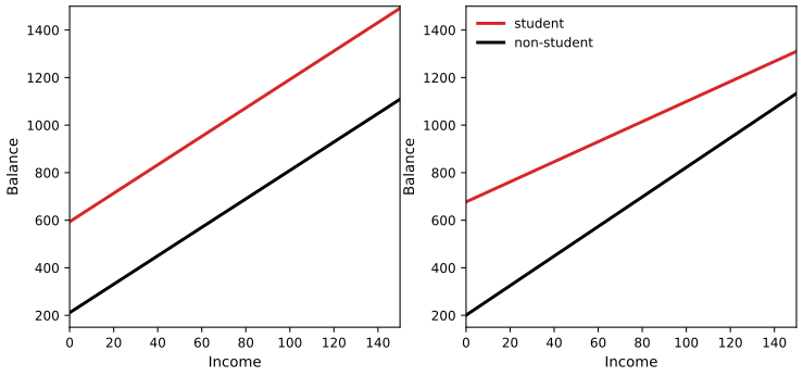
fig_3_7. Reproduces James et al. (2021), Figure 3.7. Download: PDF · SVGFilling the gap 3.10: why the hierarchical principle p. 89, “leaving them out tends to alter the meaning of the interaction”
A model with \(X_1X_2\) but without \(X_1\) forces the slope of \(X_1\) to be exactly zero when \(X_2=0\). Where zero lies on the scale of \(X_2\) is often arbitrary (a budget in dollars or above a minimum, a temperature in Celsius or Fahrenheit), so the model would change with the units. With both main effects the model is the same whatever origin is used.
Derivation
Shifting the origin. Replace \(X_2\) by \(X_2'=X_2-c\). The full model (3.31) becomes
\[ \beta_0+\beta_1X_1+\beta_2(X_2'+c)+\beta_3X_1(X_2'+c)=(\beta_0+c\beta_2)+(\beta_1+c\beta_3)X_1+\beta_2X_2'+\beta_3X_1X_2', \]again of the form (3.31): the set of possible regression functions is the same, only \(\beta_0\) and \(\beta_1\) are relabelled (and the fit, \(R^2\) and the interaction's t-test are unchanged). Now drop \(X_1\): \(\beta_0+\beta_2X_2+\beta_3X_1X_2\). In terms of \(X_2'\) it is \(\beta_0+c\beta_2+\beta_2X_2'+\beta_3X_1X_2'+c\beta_3X_1\), which contains an \(X_1\) term again. So “no main effect of \(X_1\)” is not a statement about the data but about where the zero of \(X_2\) was put.
What the main-effect coefficients mean. In (3.31), \(\beta_1\) is the slope of \(X_1\) at \(X_2=0\). In Table 3.9, \(\hat\beta_1=0.0191\) is the effect of TV in a market with no radio budget, a corner of the data. Its p-value answers that narrow question, not whether TV matters, which is why a large p-value for a main effect is no reason to drop it. Centring the predictors before forming the product makes \(\beta_1\) the slope at the average \(X_2\), and also reduces the correlation between \(X_1X_2\) and the main effects. ∎
Non-linear relationships
In the Auto data, mpg falls with horsepower along a curve (Figure 3.8). Polynomial regression adds powers of the predictor:
\[ \texttt{mpg}=\beta_0+\beta_1\times\texttt{horsepower}+\beta_2\times\texttt{horsepower}^2+\epsilon. \tag{3.36} \]This is still a linear model, with \(X_1=\texttt{horsepower}\) and \(X_2=\texttt{horsepower}^2\): it is linear in the coefficients, so ordinary least squares fits it. \(R^2\) rises from 0.606 to 0.688 and the quadratic term is highly significant (Table 3.10). A degree-5 polynomial wiggles without a clear gain. Chapter 7 develops non-linear fits further.
| Coefficient | Std. error | t-statistic | p-value | |
|---|---|---|---|---|
| Intercept | 56.9001 | 1.8004 | 31.6 | < 0.0001 |
| horsepower | −0.4662 | 0.0311 | −15.0 | < 0.0001 |
| horsepower2 | 0.0012 | 0.0001 | 10.1 | < 0.0001 |
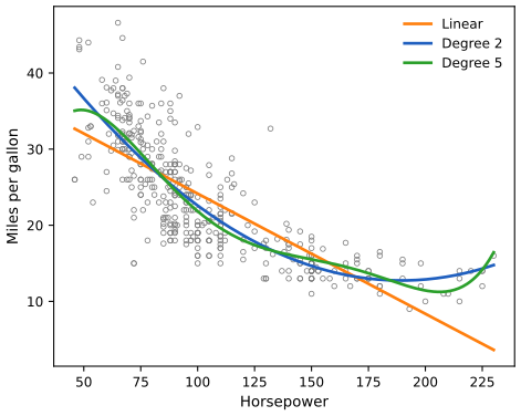
fig_3_8. Reproduces James et al. (2021), Figure 3.8. Download: PDF · SVGDeeper: Statistical Learning: Theory and Methods, Section 5.2 (piecewise polynomials and splines, which replace global polynomials).
3.3.3 Potential Problems
pp. 92–103 Six problems are common: non-linearity, correlated errors, non-constant error variance, outliers, high-leverage points and collinearity.
1. Non-linearity of the data
A residual plot (residuals \(e_i\) against the fitted values \(\hat y_i\), or against \(x_i\) in simple regression) should show no pattern. The U-shape for the linear fit of mpg on horsepower (Figure 3.9, left) reveals the curvature; the quadratic fit leaves little pattern (right). Remedies: transformations such as \(\log X\), \(\sqrt X\), \(X^2\), or the methods of Chapter 7.
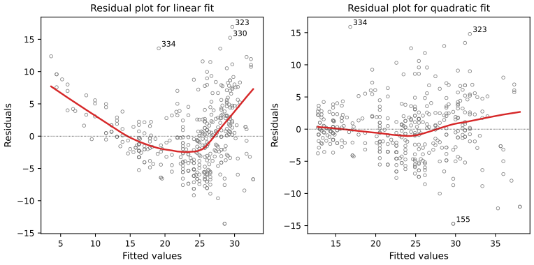
fig_3_9. Reproduces James et al. (2021), Figure 3.9; the labelled observations are the book's. Download: PDF · SVG2. Correlation of error terms
Standard errors, intervals and p-values assume uncorrelated errors. If errors are positively correlated, the computed standard errors are too small, intervals too narrow and p-values too small: unwarranted confidence. If the data were accidentally duplicated, the estimates would not change but the intervals would shrink by a factor of about \(\sqrt2\). Correlation is common in time series, where residuals plotted in time order show tracking (Figure 3.10), and wherever observations share family, diet or environment; good design is the best protection.
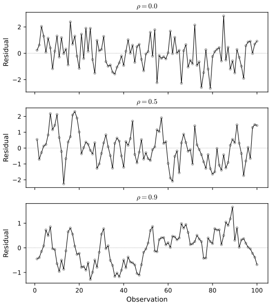
fig_3_10. Reproduces James et al. (2021), Figure 3.10. Download: PDF · SVGFilling the gap 3.12: how much correlated errors shrink the standard errors p. 94, “narrower by a factor of \(\sqrt2\)”
Duplicating the data halves \((\bX^\T\bX)^{-1}\) and barely changes \(\RSE\), so every standard error is divided by about \(\sqrt2\). For errors that follow the autoregression of Figure 3.10, the true variance of an average is larger than the naive \(\sigma^2/n\) by the factor \((1+\rho)/(1-\rho)\), which is 19 for \(\rho=0.9\).
Derivation
Duplication. Stacking the data twice turns \(\bX^\T\bX\) into \(2\bX^\T\bX\) and RSS into \(2\,\RSS\), while the residual degrees of freedom go from \(n-p-1\) to \(2n-p-1\). So \[ \SE_{\text{dup}}^2=\frac{2\RSS}{2n-p-1}\cdot\frac{(\bX^\T\bX)^{-1}_{jj}}{2}=\SE^2\cdot\frac{n-p-1}{2n-p-1}\approx\SE^2/2. \] For the Advertising regression (\(n=200\), \(p=3\)) the factor is \(\sqrt{196/396}=0.704\), close to \(1/\sqrt2=0.707\).
Autocorrelated errors. If \(\Cov(\epsilon_s,\epsilon_t)=\sigma^2\rho^{|s-t|}\), the mean of \(n\) consecutive errors has
\[ \Var(\bar\epsilon)=\frac{\sigma^2}{n^2}\sum_{s,t}\rho^{|s-t|}=\frac{\sigma^2}{n}\Big[1+2\sum_{k=1}^{n-1}\Big(1-\frac kn\Big)\rho^k\Big]\approx\frac{\sigma^2}{n}\cdot\frac{1+\rho}{1-\rho} \]for large \(n\). A standard error computed as if the errors were independent is too small by the factor \(\sqrt{(1+\rho)/(1-\rho)}\): 1.7 for \(\rho=0.5\) and 4.4 for \(\rho=0.9\). The same inflation affects the slope when the predictor also changes slowly over time. ∎
3. Non-constant variance of error terms
Often the error variance grows with the mean, heteroscedasticity, seen as a funnel in the residual plot (Figure 3.11, left). A concave transformation of the response such as \(\log Y\) or \(\sqrt Y\) shrinks the large responses more and can stabilise the variance (right). If the \(i\)th response is an average of \(n_i\) raw observations, its variance is \(\sigma^2/n_i\), and weighted least squares with weights \(w_i=n_i\) is the remedy.
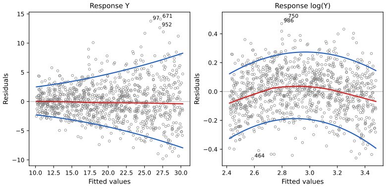
fig_3_11. Reproduces James et al. (2021), Figure 3.11. Download: PDF · SVGFilling the gap 3.13: why the log stabilises the variance, and why weights \(w_i=n_i\) pp. 96–97
If the noise is proportional to the mean, the log turns it into additive noise of constant size. If the variances are known up to a constant, weighting each squared residual by the inverse variance is the same as ordinary least squares on rescaled data with constant variance.
Derivation
The log. If \(Y=\mu(x)e^{u}\) with \(u\) of mean 0 and variance \(\tau^2\), then \(\log Y=\log\mu(x)+u\) has constant variance \(\tau^2\), while \(\Var(Y)\approx\mu(x)^2\tau^2\) grows with the mean. More generally, a first-order Taylor expansion gives \(\Var g(Y)\approx g'(\mu)^2\Var(Y)\) (the delta method): if \(\Var(Y)\propto\mu^2\), \(g=\log\) makes it constant; if \(\Var(Y)\propto\mu\) (counts), \(g=\sqrt{\ }\) does.
Weighted least squares. Suppose \(\Var(\epsilon_i)=\sigma^2/w_i\) with known \(w_i\). Multiply the \(i\)th equation by \(\sqrt{w_i}\): \(\sqrt{w_i}y_i=\sqrt{w_i}(\beta_0+\sum_j\beta_jx_{ij})+\sqrt{w_i}\epsilon_i\), and the new errors have the constant variance \(\sigma^2\). Ordinary least squares on the rescaled data minimises \(\sum_iw_i(y_i-\beta_0-\sum_j\beta_jx_{ij})^2\), and by the Gauss–Markov theorem this is the most precise linear unbiased estimator. An average of \(n_i\) uncorrelated raw observations has variance \(\sigma^2/n_i\), hence \(w_i=n_i\). ∎
Confirmed numerically on the simulated data of Figure 3.11.
4. Outliers
An outlier is a point whose \(y_i\) is far from the value the model predicts. In Figure 3.12 the outlier (observation 20) has an ordinary \(x\) value and barely moves the line, but it inflates the RSE from 0.79 to 1.09 and lowers \(R^2\) from 0.892 to 0.811, and every interval and p-value uses the RSE. To judge how large a residual is, divide it by its estimated standard error: the studentized residual. Values beyond 3 in absolute value deserve a look. Remove a point only if it is a recording error; an outlier may instead reveal a missing predictor.
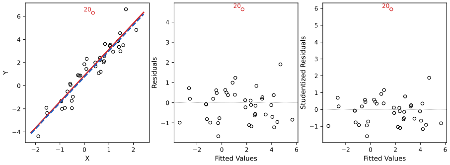
fig_3_12, outlier_data. Reproduces James et al. (2021), Figure 3.12 (the book's RSE and \(R^2\) with and without the outlier are 1.09 and 0.77, 0.805 and 0.892; ours are 1.09 and 0.79, 0.811 and 0.892). Download: PDF · SVG5. High leverage points
A point has high leverage if its \(x_i\) is unusual. Observation 41 in Figure 3.13 (left) is far to the right; removing it changes the line much more than removing the outlier did. With several predictors a point can be ordinary in each coordinate and still unusual jointly (centre). The leverage statistic of simple regression is
\[ h_i=\frac1n+\frac{(x_i-\bar x)^2}{\sum_{i'=1}^n(x_{i'}-\bar x)^2}. \tag{3.37} \]It always lies between \(1/n\) and 1, and the average leverage is \((p+1)/n\); a leverage far above \((p+1)/n\) is suspect. Observation 41 is both high-leverage and an outlier (right panel): a dangerous combination.
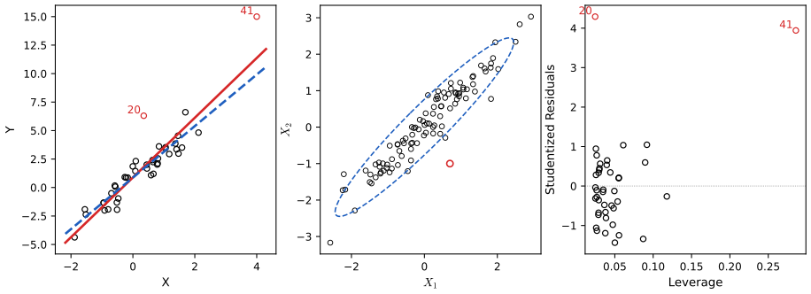
fig_3_13. Reproduces James et al. (2021), Figure 3.13. Download: PDF · SVGFilling the gap 3.11: the leverage statistic, its bounds and average, its multiple-regression form, and studentized residuals p. 99, “there is a simple extension … though we do not provide the formula here”
Leverages are the diagonal entries \(h_i\) of the hat matrix \(\bH=\bX(\bX^\T\bX)^{-1}\bX^\T\) that maps \(\by\) to \(\hat\by\): \(h_i\) is the weight of \(y_i\) in its own fitted value. In general \(h_i=\frac1n+\frac{1}{n-1}(x_i-\bar x)^\T\bS^{-1}(x_i-\bar x)\), a squared Mahalanobis distance of \(x_i\) from the centre of the data (\(\bS\) the sample covariance matrix of the predictors), which reduces to (3.37) for one predictor.
Derivation
Leverage as self-influence. \(\hat y_i=\sum_jH_{ij}y_j\), so \(h_i=H_{ii}=\partial\hat y_i/\partial y_i\): moving \(y_i\) by one unit moves its own fitted value by \(h_i\). In simple regression, the fitted value is \(\bar y+\hat\beta_1(x_i-\bar x)\) with \(\hat\beta_1=\sum_jc_jy_j\), \(c_j=(x_j-\bar x)/S_{xx}\); the coefficient of \(y_i\) is \(\frac1n+(x_i-\bar x)c_i\), which is (3.37).
Bounds and average. \(\bH\) is symmetric and \(\bH^2=\bH\). Reading the \(i\)th diagonal entry of \(\bH=\bH^2\): \(h_i=\sum_jH_{ij}^2=h_i^2+\sum_{j\ne i}H_{ij}^2\ge h_i^2\), so \(0\le h_i\le1\). With an intercept, \(\bH-\bJ\) (\(\bJ=\bone\bone^\T/n\)) is also a projection, so its diagonal entries \(h_i-1/n\) are non-negative: \(h_i\ge1/n\). Finally \[ \sum_ih_i=\tr\bH=\tr\big((\bX^\T\bX)^{-1}\bX^\T\bX\big)=p+1, \] so the average is \((p+1)/n\).
Mahalanobis form. Centre the predictors: the intercept column is orthogonal to the centred columns \(\bX_c\), so \(\bH=\bJ+\bX_c(\bX_c^\T\bX_c)^{-1}\bX_c^\T\) and \(h_i=\frac1n+(x_i-\bar x)^\T(\bX_c^\T\bX_c)^{-1}(x_i-\bar x)\), with \(\bX_c^\T\bX_c=(n-1)\bS\). A point far from the centre in the metric of \(\bS^{-1}\) has high leverage even if no single coordinate is extreme: in the centre panel of Figure 3.13 the red point lies across the narrow direction of the cloud.
Residuals of high-leverage points are small. The residual vector is \((\bI-\bH)\boldsymbol\epsilon\), so \(\Var(e_i)=\sigma^2(1-h_i)\). A point with \(h_i\) near 1 drags the fit to itself and leaves a residual near 0, which is why raw residual plots miss it. The studentized residual divides by the right standard error,
\[ t_i=\frac{e_i}{\hat\sigma_{(i)}\sqrt{1-h_i}}, \]where \(\hat\sigma_{(i)}\) is the RSE of the fit without observation \(i\) (so that an outlier does not inflate its own yardstick). Under the model with normal errors \(t_i\) has a t-distribution with \(n-p-2\) degrees of freedom, so \(|t_i|>3\) is rare for any single point. (R's rstudent and statsmodels' resid_studentized_external compute this \(t_i\).) Cook's distance \(D_i=\frac{e_i^2}{(p+1)\RSE^2}\cdot\frac{h_i}{(1-h_i)^2}\) combines both and measures how far all fitted values move when \(i\) is deleted: 2.27 for observation 41, 0.16 for observation 20. ∎
Confirmed numerically: (3.37) equals the diagonal of \(\bH\), the bounds and the average hold, and the studentized residuals and Cook's distances agree with statsmodels.
Deeper: Statistical Learning: Theory and Methods, Result 3.2 (the hat matrix is an orthogonal projection, with eigenvalues 0 and 1).
6. Collinearity
Collinearity means two or more predictors are closely related. In the Credit data, limit and age are unrelated, but limit and rating are almost proportional (Figure 3.14). Collinear predictors are hard to separate: in the RSS contours for balance on limit and rating (Figure 3.15, right) many coefficient pairs fit almost equally well, along a narrow valley. Collinearity inflates the standard errors, shrinks the t-statistics and lowers the power of the tests (the probability of detecting a non-zero coefficient). In Table 3.11 the standard error of the limit coefficient grows 12-fold when rating replaces age, and its p-value rises to 0.701: the importance of limit is masked.
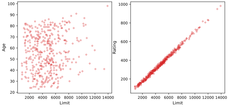
fig_3_14. Reproduces James et al. (2021), Figure 3.14. Download: PDF · SVG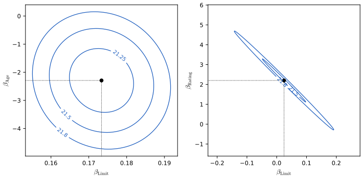
fig_3_15, profile_rss. Reproduces James et al. (2021), Figure 3.15. Download: PDF · SVG| Coefficient | Std. error | t-statistic | p-value | ||
|---|---|---|---|---|---|
| Model 1 | Intercept | −173.411 | 43.828 | −3.957 | < 0.0001 |
| age | −2.292 | 0.672 | −3.407 | 0.0007 | |
| limit | 0.173 | 0.005 | 34.496 | < 0.0001 | |
| Model 2 | Intercept | −377.537 | 45.254 | −8.343 | < 0.0001 |
| rating | 2.202 | 0.952 | 2.312 | 0.0213 | |
| limit | 0.025 | 0.064 | 0.384 | 0.7012 |
The correlation matrix detects collinearity between pairs but not multicollinearity among three or more variables. The variance inflation factor does: the ratio of the variance of \(\hat\beta_j\) in the full model to its variance when \(X_j\) is fitted alone,
\[ \VIF(\hat\beta_j)=\frac{1}{1-R^2_{X_j|X_{-j}}}, \]where \(R^2_{X_j|X_{-j}}\) is the \(R^2\) of the regression of \(X_j\) on all other predictors. The minimum is 1; values above 5 or 10 signal trouble. Balance on age, rating and limit gives VIFs 1.01, 160.67 and 160.59. Two remedies: drop one of the collinear variables (without rating, \(R^2\) goes from 0.754 to 0.750 and the VIFs are 1.01), or combine them, e.g. the average of standardised limit and rating as a measure of credit-worthiness.
Filling the gap 3.14: why the VIF is \(1/(1-R^2_{X_j|X_{-j}})\), and what it does to the standard error p. 102
From the adjusted-predictor formula of Filling the gap 3.5, \(\Var(\hat\beta_j)=\sigma^2/\sum_ir_{ij}^2\), and the residual sum of squares of \(x_j\) on the others is \(S_{x_jx_j}(1-R^2_{X_j|X_{-j}})\). The standard error is therefore multiplied by \(\sqrt{\VIF}\), with the same \(\sigma\) in both models.
Derivation
The ratio. Alone, \(\Var(\hat\beta_j)=\sigma^2/S_{x_jx_j}\) by (3.8). In the full model, \(\Var(\hat\beta_j)=\sigma^2/\sum_ir_{ij}^2\), and by the definition of \(R^2\) for the regression of \(x_j\) on the other predictors, \(\sum_ir_{ij}^2=\RSS_{x_j}=(1-R^2_{X_j|X_{-j}})\,S_{x_jx_j}\). Dividing,
\[ \frac{\Var(\hat\beta_j)\ \text{full}}{\Var(\hat\beta_j)\ \text{alone}}=\frac{S_{x_jx_j}}{\RSS_{x_j}}=\frac{1}{1-R^2_{X_j|X_{-j}}}. \]The ratio is a property of the predictors alone, with the same \(\sigma^2\) in numerator and denominator; the estimated variances use different RSEs in the two fits, so their ratio differs slightly from the VIF.
Two predictors. \(R^2_{X_1|X_2}=r_{12}^2\), so \(\VIF=1/(1-r_{12}^2)\) for both. Limit and rating have \(r=0.9969\), so each has \(\VIF=160.5\) in Model 2 of Table 3.11 and \(\sqrt{160.5}=12.7\): the 12-fold increase of the standard error of limit (exactly \(0.0638/0.0050=12.7\)). The values 160.67 and 160.59 quoted by the book are for the three-predictor model with age, which is almost uncorrelated with both.
Why the valley in Figure 3.15. The RSS contours are the ellipses \((\bb-\hb)^\T\bX_c^\T\bX_c(\bb-\hb)=\text{const}\); for standardised predictors \(\bX_c^\T\bX_c\propto\begin{pmatrix}1&r\\r&1\end{pmatrix}\), whose eigenvalues \(1\pm r\) give axes in the ratio \(\sqrt{(1+r)/(1-r)}\), about 25 for \(r=0.997\). ∎
Confirmed numerically: the VIF equals the ratio of the diagonal entries of \((\bX^\T\bX)^{-1}\) times \(S_{x_jx_j}\); the values 1.005, 1.145, 1.145 (Advertising) and 1.01, 160.67, 160.59 (Credit) are reproduced.
3.4 The Marketing Plan
pp. 103–105 The seven questions, answered for the Advertising data:
- Is there a relationship? Yes: the F-test of \(H_0:\beta_{\text{TV}}=\beta_{\text{radio}}=\beta_{\text{newspaper}}=0\) has \(F=570\) and a p-value near \(10^{-96}\).
- How strong? \(\RSE=1.69\) against a mean of 14.022, a typical error of about 12%; the predictors explain almost 90% of the variance of sales (\(R^2=0.897\)).
- Which media? TV and radio (tiny p-values in Table 3.4); not newspaper, once TV and radio are known. Chapter 6 returns to this question.
- How large is each association? 95% intervals (0.043, 0.049) for TV, (0.172, 0.206) for radio and (\(-0.013\), 0.011) for newspaper. The VIFs (1.005, 1.145, 1.145) rule out collinearity as the reason for newspaper's wide interval. Separately (Tables 3.1 and 3.3) TV and radio are strongly associated with sales, and newspaper mildly.
- How accurately can we predict? With a prediction interval for an individual market and a confidence interval for the average over many markets (Filling the gap 3.8).
- Is the relationship linear? Not quite: the residuals of Figure 3.5 show a pattern; transformations or interactions can capture it.
- Is there synergy? Yes: the TV×radio interaction raises \(R^2\) from about 90% to almost 97% (Table 3.9).
3.5 Comparison of Linear Regression with K-Nearest Neighbors
pp. 105–110 Linear regression is parametric: it assumes a form for \(f\), which makes it easy to fit and interpret and allows tests, but fails if the form is far from the truth. Non-parametric methods assume no form.
Definition 3.4 (K-nearest-neighbours regression) p. 105
Given \(K\) and a point \(x_0\), let \(\mathcal N_0\) be the \(K\) training observations closest to \(x_0\). Then
\[ \hat f(x_0)=\frac1K\sum_{x_i\in\mathcal N_0}y_i. \]\(K=1\) interpolates the training data with a step function; larger \(K\) averages more points and gives a smoother, less variable but more biased fit (Figure 3.16). \(K\) is chosen by estimating the test error (Chapter 5).
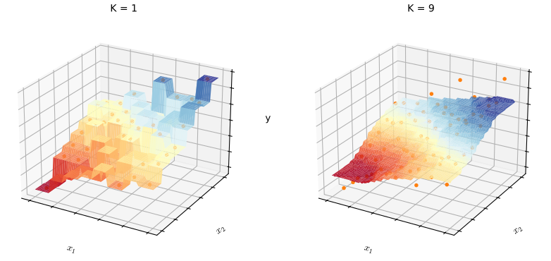
fig_3_16, knn_reg. Reproduces James et al. (2021), Figure 3.16. Download: PDF · SVGWhich wins? The parametric method, whenever its form is close to the truth. With a linear \(f\) (Figures 3.17 and 3.18) least squares beats KNN for every \(K\), only slightly for large \(K\) and badly for \(K=1\). As \(f\) becomes non-linear (Figure 3.19), the error of least squares grows while that of KNN hardly changes, and KNN wins. But with more predictors (Figure 3.20), extra noise inputs barely hurt least squares and ruin KNN, because in high dimensions the nearest neighbours are far away: the curse of dimensionality. As a rule, parametric methods win when there are few observations per predictor, and linear regression may be preferred anyway for its interpretability.
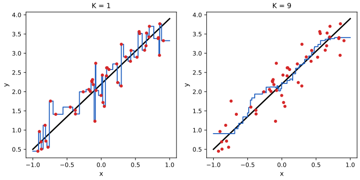
fig_3_17. Reproduces James et al. (2021), Figure 3.17. Download: PDF · SVG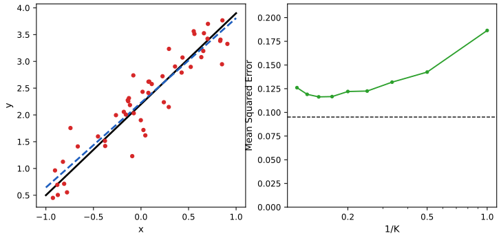
fig_3_18. Reproduces James et al. (2021), Figure 3.18. Download: PDF · SVG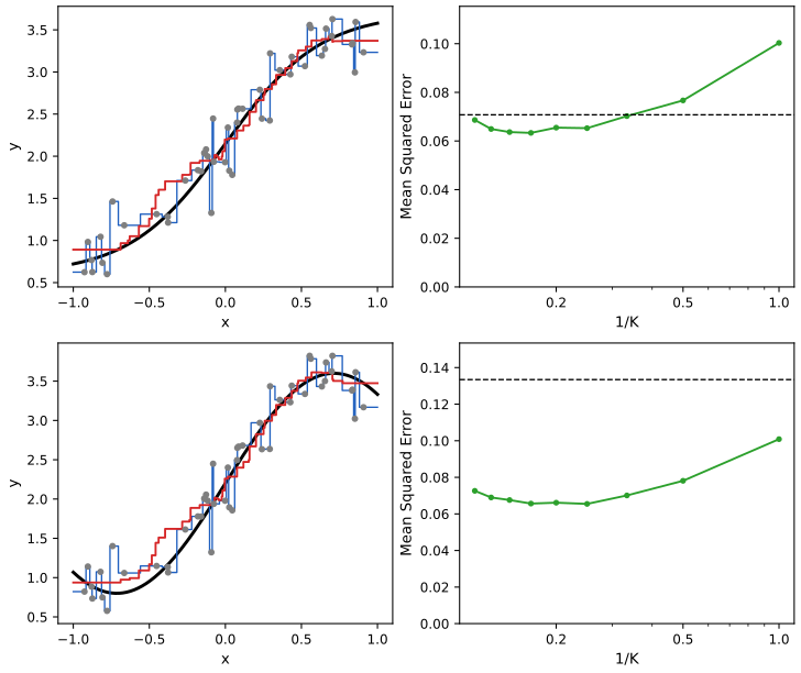
fig_3_19. Reproduces James et al. (2021), Figure 3.19 (the book reports KNN ahead for \(K\ge4\) in the top row). Download: PDF · SVG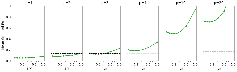
fig_3_20. Reproduces James et al. (2021), Figure 3.20. Download: PDF · SVGFilling the gap 3.15: the bias and variance of KNN, and why it suffers in high dimensions pp. 106–110
At a test point, KNN's expected squared error is \(\sigma^2\) (irreducible) plus a squared bias that grows with the size of the neighbourhood plus a variance \(\sigma^2/K\). In \(p\) dimensions, a neighbourhood holding a fixed fraction of the data must stretch over almost the whole range of every input.
Derivation
Bias and variance. Fix the training inputs and a test point \(x_0\) with \(Y_0=f(x_0)+\epsilon_0\). Since \(\hat f(x_0)=\frac1K\sum_{\ell\in\mathcal N_0}(f(x_\ell)+\epsilon_\ell)\) with independent errors,
\[ \E\big(Y_0-\hat f(x_0)\big)^2=\sigma^2+\Big(f(x_0)-\frac1K\sum_{\ell\in\mathcal N_0}f(x_\ell)\Big)^2+\frac{\sigma^2}{K}. \]For \(K=1\) and a smooth \(f\) with close neighbours, this is about \(2\sigma^2\): in Figure 3.18, \(0.186\approx2\times0.09\). Increasing \(K\) lowers the variance term and raises the bias term. For least squares with a correct linear model the excess over \(\sigma^2\) is on average about \(\sigma^2(p+1)/n\) at the training inputs, which is why it is hard to beat when \(f\) is linear (0.095 against \(\sigma^2=0.09\)).
The curse of dimensionality. Take \(n\) points uniform on the cube \([-1,1]^p\). A sub-cube that contains a fraction \(s\) of the volume (so about \(sn\) points) has edge \(s^{1/p}\) times the full edge. With \(n=50\) and \(K=9\), \(s=0.18\): the edge fraction is 0.18 for \(p=1\), 0.42 for \(p=2\), 0.65 for \(p=4\), 0.84 for \(p=10\) and 0.92 for \(p=20\). The “local” average then mixes points with very different values of the one input that matters, and the bias term explodes, as in Figure 3.20. Least squares only needs to estimate one coefficient per input, and the useless ones cost about \(\sigma^2/n\) each. ∎
Deeper: Statistical Learning: Theory and Methods, Section 2.3 (least squares and nearest neighbours as the two extremes) and Section 2.5 (local methods in high dimensions); Section 7.3 (the bias–variance decomposition of KNN and of linear fits).
See also (companion courses): Bayesian and Probabilistic Machine Learning, Section 1.4 and Statistical Methods for Modern Biology, Section 12.4.2 (the curse of dimensionality).
3.6 Lab: Linear Regression (R and Python)
pp. 110–121 The lab follows the R lab of James et al. (2021) and the Python lab of James et al. (2023), which do the same analyses: simple and multiple regression of the median house value in the Boston data, diagnostics, interactions, polynomial and log terms, and qualitative predictors in the Carseats data. The code below is my own, in ch03_lab.R and ch03_lab.py; each pair of boxes is one step, R on the left and Python on the right (stacked on a phone). The two scripts give the same numbers to every printed digit. The Python lab of the book builds its model matrices with its own helper package; here plain statsmodels (with formulas) and pandas are used instead, so the Python code runs with standard packages only.
3.6.1 Libraries
R needs the ISLR2 package for the data and car for vif(); Python needs numpy, pandas, matplotlib, scipy and statsmodels, and reads the book's CSV files with isl_data() from the course's common.py. The import blocks are at the top of each script.
3.6.2 Simple Linear Regression
The Boston data record the median house value medv (thousands of dollars) and 12 predictors for 506 census tracts, among them rm (average rooms per house), age (share of houses built before 1940) and lstat (percentage of households of low socioeconomic status).
R
dim(Boston)                      # 506 census tracts, 12 predictors and the response medv
names(Boston)
Python
Boston = isl_data("Boston", index_col=0)
print(Boston.shape)              # 506 census tracts, 12 predictors and the response medv
print(list(Boston.columns))
Regress medv on lstat. In R the model is a formula; in Python sm.OLS takes the response and an explicit model matrix, here built with a column of ones.
R
lm.fit <- lm(medv ~ lstat, data = Boston)
summary(lm.fit)
Python
X = sm.add_constant(Boston[["lstat"]])        # the model matrix: a column of ones and lstat
y = Boston["medv"]
results = sm.OLS(y, X).fit()
print(results.summary().tables[1])
print("RSE %.3f on %d df, R2 %.4f, F %.1f" % (np.sqrt(results.scale), results.df_resid, results.rsquared, results.fvalue))
Estimate Std. Error t value Pr(>|t|) (Intercept) 34.55384 0.56263 61.41 <2e-16 lstat -0.95005 0.03873 -24.53 <2e-16 Residual standard error: 6.216 on 504 degrees of freedom Multiple R-squared: 0.5441, F-statistic: 601.6 on 1 and 504 DF
Python prints the same table (const 34.5538, lstat −0.9500, t −24.528) and “RSE 6.216 on 504 df, R2 0.5441, F 601.6”.
R
coef(lm.fit)
confint(lm.fit)                  # 95% intervals: estimate -/+ t(0.975, 504) * SE
c(RSE = summary(lm.fit)$sigma, R2 = summary(lm.fit)$r.squared)
Python
print(results.params)
print(results.conf_int(alpha=0.05))           # estimate -/+ t(0.975, 504) * SE
print(pd.Series({"RSE": np.sqrt(results.scale), "R2": results.rsquared}))
2.5 % 97.5 % (Intercept) 33.448457 35.6592247 lstat -1.026148 -0.8739505
Confidence and prediction intervals at lstat = 5, 10 and 15 (Filling the gap 3.8): both are centred at the same fitted values, and the prediction intervals are much wider.
R
new <- data.frame(lstat = c(5, 10, 15))
predict(lm.fit, new, interval = "confidence")
predict(lm.fit, new, interval = "prediction")
Python
new = sm.add_constant(pd.DataFrame({"lstat": [5, 10, 15]}), has_constant="add")
pred = results.get_prediction(new).summary_frame(alpha=0.05)
print(pred[["mean", "mean_ci_lower", "mean_ci_upper"]])   # confidence intervals for f(x0)
print(pred[["mean", "obs_ci_lower", "obs_ci_upper"]])     # prediction intervals for Y at x0
fit conf. lwr conf. upr pred. lwr pred. upr 1 29.80359 29.00741 30.59978 17.565675 42.04151 2 25.05335 24.47413 25.63256 12.827626 37.27907 3 20.30310 19.73159 20.87461 8.077742 32.52846
Both languages print these numbers (R as two tables from predict, Python as two column sets of summary_frame).
R
png(file.path(out_dir, "lab-r-fit.png"), width = 640, height = 480, res = 110)
plot(Boston$lstat, Boston$medv, pch = 20, col = "grey40", xlab = "lstat", ylab = "medv")
abline(lm.fit, lwd = 3, col = "red")
invisible(dev.off())
Python
fig, ax = plt.subplots(figsize=(5.8, 4.3))
ax.scatter(Boston["lstat"], Boston["medv"], s=8, color="0.4")
ax.axline((0, results.params["const"]), slope=results.params["lstat"], color="red", lw=3)
ax.set_xlabel("lstat")
ax.set_ylabel("medv")
save(fig, "lab-py-fit")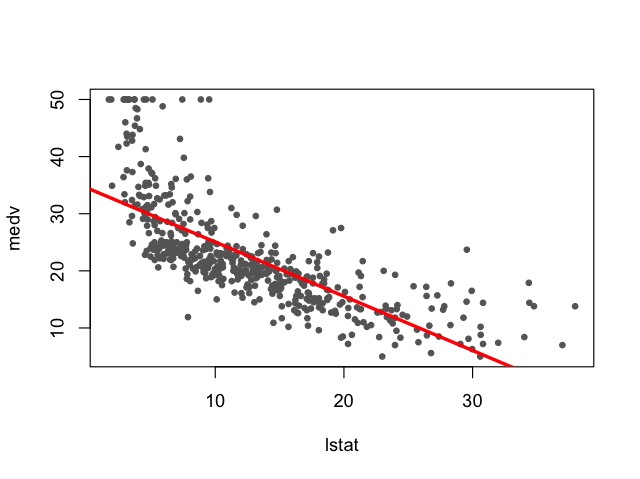
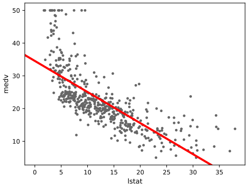
Left: R (lab-r-fit.png); right: Python (lab-py-fit.svg). The points bend away from the line at both ends: the relation is not linear, which the lab takes up in Section 3.6.5.
Diagnostic plots. R draws four standard panels with plot(lm.fit); in Python the same four panels are written as a short function.
R
png(file.path(out_dir, "lab-r-diagnostics.png"), width = 900, height = 800, res = 110)
par(mfrow = c(2, 2))
plot(lm.fit)                     # residuals, normal Q-Q, scale-location, residuals vs leverage
invisible(dev.off())
Python
def diagnostics(fit, name):
    """The four panels that R draws for plot(lm.fit)."""
    infl = fit.get_influence()
    r_std = infl.resid_studentized_internal
    h = infl.hat_matrix_diag
    fv = fit.fittedvalues
    fig, ax = plt.subplots(2, 2, figsize=(8.4, 7.4))
    ax[0, 0].scatter(fv, fit.resid, s=8, facecolors="none", edgecolors="0.3")
    ax[0, 0].plot(*lowess(fit.resid, fv, frac=2 / 3).T, color="red")
    ax[0, 0].set(xlabel="Fitted values", ylabel="Residuals", title="Residuals vs Fitted")
    sm.qqplot(r_std, line="45", ax=ax[0, 1], markersize=3)
    ax[0, 1].set(title="Normal Q-Q", ylabel="Standardized residuals")
    ax[1, 0].scatter(fv, np.sqrt(np.abs(r_std)), s=8, facecolors="none", edgecolors="0.3")
    ax[1, 0].plot(*lowess(np.sqrt(np.abs(r_std)), fv, frac=2 / 3).T, color="red")
    ax[1, 0].set(xlabel="Fitted values", ylabel=r"$\sqrt{|\mathrm{standardized\ residual}|}$", title="Scale-Location")
    ax[1, 1].scatter(h, r_std, s=8, facecolors="none", edgecolors="0.3")
    ax[1, 1].set(xlabel="Leverage", ylabel="Standardized residuals", title="Residuals vs Leverage")
    fig.tight_layout()
    save(fig, name)


diagnostics(results, "lab-py-diagnostics")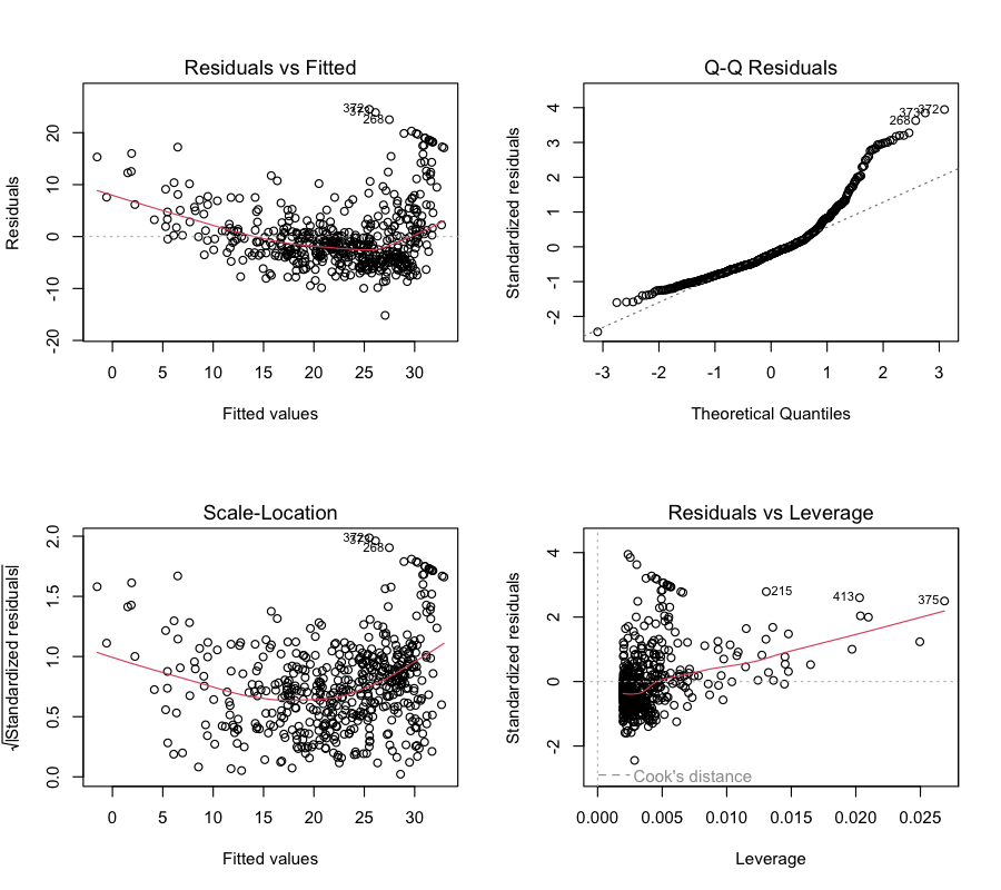
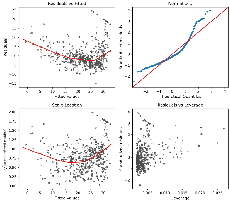
medv on lstat, R (left) and Python (right). The U-shaped smooth in the residual plot shows non-linearity; the upper tail of the Q-Q plot shows a few large positive residuals (tracts whose values are much higher than the line predicts). Download: R (PNG) · Python (SVG)R
h <- hatvalues(lm.fit)
which.max(h)                     # observation 375 (R counts from 1)
max(h)
head(sort(abs(rstudent(lm.fit)), decreasing = TRUE), 3)
Python
infl = results.get_influence()
h = infl.hat_matrix_diag
print(np.argmax(h), h.max())                  # index 374: Python counts from 0 (R says 375)
r_stud = pd.Series(infl.resid_studentized_external, index=Boston.index)
print(r_stud.abs().sort_values(ascending=False).head(3))
R: which.max(h) = 375, max(h) = 0.02686517; largest |studentized|: 372 4.0047, 373 3.9010, 268 3.6723 Python: np.argmax(h) = 374, h.max() = 0.026865166510283492; 372 4.004703, 373 3.901020, 268 3.672331
numpy from 0. The row labels of the data frame (here 1 to 506 in both, read from the file) avoid the confusion, which is why the studentized residuals carry the same labels 372, 373, 268 in both languages.3.6.3 Multiple Linear Regression
R
lm.fit <- lm(medv ~ lstat + age, data = Boston)
summary(lm.fit)$coefficients
Python
results1 = smf.ols("medv ~ lstat + age", data=Boston).fit()
print(coefs(results1))
Estimate Std. Error t value Pr(>|t|) (Intercept) 33.22276053 0.73084711 45.457881 2.94e-180 lstat -1.03206856 0.04819073 -21.416330 8.42e-73 age 0.03454434 0.01222547 2.825605 4.91e-03
All 12 predictors at once: medv ~ . in R; in Python the formula is assembled from the column names.
R
lm.fit <- lm(medv ~ ., data = Boston)
summary(lm.fit)
c(R2 = summary(lm.fit)$r.squared, RSE = summary(lm.fit)$sigma)
Python
terms = Boston.columns.drop("medv")
results = smf.ols("medv ~ " + " + ".join(terms), data=Boston).fit()
print(coefs(results))
print("RSE %.3f on %d df, R2 %.4f, adjusted R2 %.4f, F %.1f" % (np.sqrt(results.scale), results.df_resid, results.rsquared, results.rsquared_adj, results.fvalue))
Estimate Std. Error t value Pr(>|t|) (Intercept) 41.617270 4.936039 8.431 3.79e-16 crim -0.121389 0.033000 -3.678 0.000261 zn 0.046963 0.013879 3.384 0.000772 indus 0.013468 0.062145 0.217 0.828520 chas 2.839993 0.870007 3.264 0.001173 nox -18.758022 3.851355 -4.870 1.50e-06 rm 3.658119 0.420246 8.705 < 2e-16 age 0.003611 0.013329 0.271 0.786595 dis -1.490754 0.201623 -7.394 6.17e-13 rad 0.289405 0.066908 4.325 1.84e-05 tax -0.012682 0.003801 -3.337 0.000912 ptratio -0.937533 0.132206 -7.091 4.63e-12 lstat -0.552019 0.050659 -10.897 < 2e-16 Residual standard error: 4.798 on 493 degrees of freedom Multiple R-squared: 0.7343, Adjusted R-squared: 0.7278, F-statistic: 113.5 on 12 and 493 DF
Variance inflation factors (Filling the gap 3.14): moderate, the largest for tax (9.0) and rad (7.4), which are strongly correlated.
R
round(vif(lm.fit), 3)Python
Xall = sm.add_constant(Boston[terms])
vif = pd.Series([variance_inflation_factor(Xall.values, i) for i in range(1, Xall.shape[1])], index=terms)
print(vif.round(3))
crim zn indus chas nox rm age dis rad tax ptratio lstat 1.767 2.298 3.987 1.071 4.369 1.913 3.088 3.954 7.445 9.002 1.797 2.871
car::vif takes the fitted model. statsmodels' variance_inflation_factor takes a model matrix and a column index and regresses that column on all other columns of the matrix; the matrix must therefore include the column of ones (otherwise the auxiliary regressions have no intercept and the VIFs are wrong), and that column is skipped in the loop.Dropping age, whose p-value is 0.79:
R
lm.fit1 <- update(lm.fit, ~ . - age)          # the same as lm(medv ~ . - age, data = Boston)
round(summary(lm.fit1)$coefficients, 4)
Python
minus_age = terms.drop("age")
print(coefs(smf.ols("medv ~ " + " + ".join(minus_age), data=Boston).fit()))
Output (both): 11 coefficients, e.g. lstat −0.5474 (SE 0.0477) and rm 3.6811 (SE 0.4112).
update(lm.fit, ~ . - age) refits a stored model with one term removed; in Python one rebuilds the formula from the list of names without age.3.6.4 Interaction Terms
lstat * age is shorthand for lstat + age + lstat:age in both formula languages.
R
summary(lm(medv ~ lstat * age, data = Boston))$coefficientsPython
print(coefs(smf.ols("medv ~ lstat * age", data=Boston).fit(), 6))Estimate Std. Error t value Pr(>|t|) (Intercept) 36.0885359346 1.469835463 24.55277263 4.907116e-88 lstat -1.3921168406 0.167455532 -8.31335236 8.780730e-16 age -0.0007208595 0.019879171 -0.03626205 9.710878e-01 lstat:age 0.0041559518 0.001851795 2.24428275 2.524911e-02
The interaction is significant at 5% (p = 0.025) while the main effect of age is not (p = 0.97); the hierarchical principle (Filling the gap 3.10) keeps age in the model.
3.6.5 Non-linear Transformations of the Predictors
A quadratic term needs protection inside a formula: I(lstat^2) in R, I(lstat**2) in Python. The two nested models are compared by the F-test (3.24).
R
lm.fit <- lm(medv ~ lstat, data = Boston)
lm.fit2 <- lm(medv ~ lstat + I(lstat^2), data = Boston)
summary(lm.fit2)$coefficients
anova(lm.fit, lm.fit2)
Python
lm_fit = smf.ols("medv ~ lstat", data=Boston).fit()
lm_fit2 = smf.ols("medv ~ lstat + I(lstat**2)", data=Boston).fit()
print(coefs(lm_fit2, 5))
print(anova_lm(lm_fit, lm_fit2))
Estimate Std. Error t value Pr(>|t|) (Intercept) 42.86200733 0.872084393 49.14892 3.500749e-194 lstat -2.33282110 0.123803305 -18.84296 2.548861e-60 I(lstat^2) 0.04354689 0.003745149 11.62755 7.630116e-28 Model 1: medv ~ lstat Model 2: medv ~ lstat + I(lstat^2) Res.Df RSS Df Sum of Sq F Pr(>F) 1 504 19472 2 503 15347 1 4125.1 135.2 < 2.2e-16
Python's anova_lm prints the same rows: residual sums of squares 19472.38 and 15347.24, F = 135.199822, p = 7.63e-28 (R only prints “< 2.2e-16”). Since the models differ by one term, \(F=11.62755^2\), the squared t of the quadratic term.
The Python edition of the book compares lstat + age with an orthogonal quadratic in lstat plus age. Both languages:
R
lm.fit.a <- lm(medv ~ lstat + age, data = Boston)
lm.fit.q <- lm(medv ~ poly(lstat, 2) + age, data = Boston)
summary(lm.fit.q)$coefficients
anova(lm.fit.a, lm.fit.q)
Python
P2 = poly(Boston["lstat"], 2)
B2 = Boston.assign(p1=P2[:, 0], p2=P2[:, 1])
results3 = smf.ols("medv ~ p1 + p2 + age", data=B2).fit()
print(coefs(results3))
print(anova_lm(results1, results3))
Estimate Std. Error t value Pr(>|t|) (Intercept) 17.71511297 0.78105479 22.681012 6.291878e-79 poly(lstat, 2)1 -179.22786953 6.73275761 -26.620277 5.093315e-98 poly(lstat, 2)2 72.99075535 5.48200559 13.314608 7.468491e-35 age 0.07025447 0.01085673 6.471052 2.316450e-10 Res.Df RSS Df Sum of Sq F Pr(>F) 1 503 19168 2 502 14166 1 5002.5 177.28 < 2.2e-16
poly(x, d) returns orthogonal polynomials (columns that are uncorrelated and of unit length), which are numerically stable. statsmodels has no such function, so ch03_lab.py defines poly() by the same recipe (a QR decomposition of the centred powers \(1,x,\dots,x^d\), each column scaled to unit length); it reproduces R's basis exactly, including signs, so the coefficients agree to all digits (\(-179.2279\), 72.9908).R
png(file.path(out_dir, "lab-r-diagnostics-quad.png"), width = 900, height = 800, res = 110)
par(mfrow = c(2, 2))
plot(lm.fit2)
invisible(dev.off())
Python
diagnostics(lm_fit2, "lab-py-diagnostics-quad")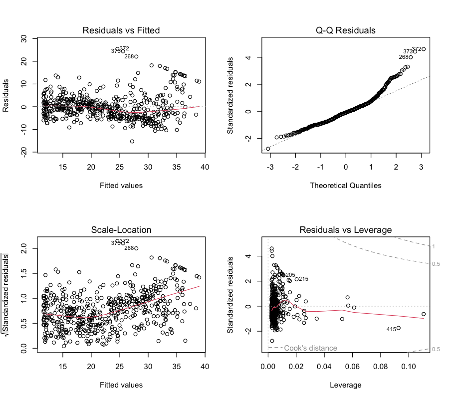
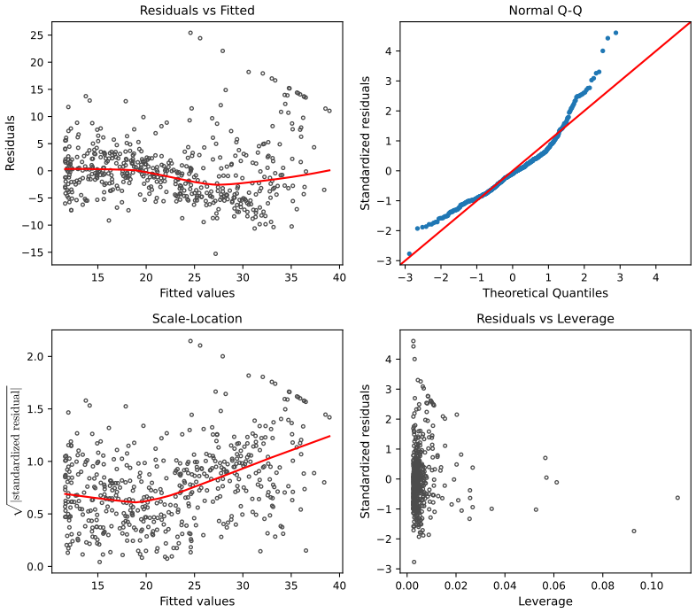
A fifth-degree polynomial, and a log transformation of rm:
R
lm.fit5 <- lm(medv ~ poly(lstat, 5), data = Boston)
summary(lm.fit5)$coefficients
raw5 <- lm(medv ~ poly(lstat, 5, raw = TRUE), data = Boston)
max(abs(fitted(lm.fit5) - fitted(raw5)))      # same fitted values, different coefficients
Python
P5 = pd.DataFrame(poly(Boston["lstat"], 5), columns=["p%d" % k for k in range(1, 6)], index=Boston.index)
lm_fit5 = sm.OLS(Boston["medv"], sm.add_constant(P5)).fit()
print(coefs(lm_fit5))
raw5 = smf.ols("medv ~ lstat + I(lstat**2) + I(lstat**3) + I(lstat**4) + I(lstat**5)", data=Boston).fit()
print(np.abs(lm_fit5.fittedvalues - raw5.fittedvalues).max())   # same fitted values, different coefficients
Estimate Std. Error t value Pr(>|t|) (Intercept) 22.53281 0.2318258 97.197129 0.000000e+00 poly(lstat, 5)1 -152.45955 5.2147934 -29.235971 2.692129e-110 poly(lstat, 5)2 64.22724 5.2147934 12.316354 1.252507e-30 poly(lstat, 5)3 -27.05110 5.2147934 -5.187377 3.104349e-07 poly(lstat, 5)4 25.45173 5.2147934 4.880679 1.424119e-06 poly(lstat, 5)5 -19.25242 5.2147934 -3.691885 2.470868e-04 R: max |fitted difference|, orthogonal vs raw = 1.8e-12; Python: 1.4e-07
lm uses a pivoted QR decomposition, statsmodels a pseudo-inverse. This is the practical reason for orthogonal polynomials. All standard errors equal 5.2148 because the orthogonal columns have unit length: each SE is just the RSE.R
summary(lm(medv ~ log(rm), data = Boston))$coefficientsPython
print(coefs(smf.ols("medv ~ np.log(rm)", data=Boston).fit()))Estimate Std. Error t value Pr(>|t|) (Intercept) -76.48782 5.027725 -15.21321 2.767277e-43 log(rm) 54.05457 2.739460 19.73183 1.217208e-64
3.6.6 Qualitative Predictors
The Carseats data give child car seat sales (thousands of units) at 400 stores, with qualitative predictors such as ShelveLoc (quality of the shelf location: Bad, Medium, Good), Urban and US. Both languages create the dummy variables of Definition 3.3 automatically.
R
dim(Carseats)
lm.fit <- lm(Sales ~ . + Income:Advertising + Price:Age, data = Carseats)
summary(lm.fit)
Python
Carseats = isl_data("Carseats")
print(Carseats.shape)
allvars = Carseats.columns.drop("Sales")
formula = "Sales ~ " + " + ".join(allvars) + " + Income:Advertising + Price:Age"
fit_cs = smf.ols(formula, data=Carseats).fit()
print(coefs(fit_cs))
print("RSE %.3f on %d df, R2 %.4f, F %.1f" % (np.sqrt(fit_cs.scale), fit_cs.df_resid, fit_cs.rsquared, fit_cs.fvalue))
Estimate Std. Error t value Pr(>|t|) (Intercept) 6.5755654 1.0087470 6.519 2.22e-10 CompPrice 0.0929371 0.0041183 22.567 < 2e-16 Income 0.0108940 0.0026044 4.183 3.57e-05 Advertising 0.0702462 0.0226091 3.107 0.002030 Population 0.0001592 0.0003679 0.433 0.665330 Price -0.1008064 0.0074399 -13.549 < 2e-16 ShelveLocGood 4.8486762 0.1528378 31.724 < 2e-16 ShelveLocMedium 1.9532620 0.1257682 15.531 < 2e-16 Age -0.0579466 0.0159506 -3.633 0.000318 Education -0.0208525 0.0196131 -1.063 0.288361 UrbanYes 0.1401597 0.1124019 1.247 0.213171 USYes -0.1575571 0.1489234 -1.058 0.290729 Income:Advertising 0.0007510 0.0002784 2.698 0.007290 Price:Age 0.0001068 0.0001333 0.801 0.423812 Residual standard error: 1.011 on 386 degrees of freedom Multiple R-squared: 0.8761, F-statistic: 210 on 13 and 386 DF
R
contrasts(Carseats$ShelveLoc)Python
levels = sorted(Carseats["ShelveLoc"].unique())            # Bad, Good, Medium: Bad is the baseline
print(pd.get_dummies(pd.Categorical(levels, categories=levels), drop_first=True, dtype=int).set_axis(levels))
Good Medium Bad 0 0 Good 1 0 Medium 0 1
Bad is the baseline. A good shelf location goes with 4.85 thousand more units than a bad one, a medium one with 1.95 thousand more, other things equal.
ShelveLoc[T.Good] (T for treatment coding), while R keeps the order of the formula and writes ShelveLocGood. In both, the baseline is the first level in alphabetical order (Bad). Neither prints a contrast matrix in the same way: R's contrasts() shows it directly, and in Python it is reconstructed above with pd.get_dummies(..., drop_first=True).3.6.7 Writing Functions
The R lab writes a function that loads the libraries; the Python lab writes abline(), which adds a line with given intercept and slope to a plot (R has abline built in, and matplotlib has ax.axline, used in the plot step above).
R
LoadLibraries <- function() {
  library(ISLR2)
  library(car)
  print("The libraries have been loaded.")
}
LoadLibraries()
Python
def abline(ax, b, m, *args, **kwargs):
    "Add the line with intercept b and slope m to the axes ax."
    xlim = ax.get_xlim()
    ax.plot(xlim, [b + m * xlim[0], b + m * xlim[1]], *args, **kwargs)


fig, ax = plt.subplots(figsize=(5.8, 4.3))
ax.scatter(Boston["lstat"], Boston["medv"], s=8, color="0.4")
abline(ax, lm_fit.params["Intercept"], lm_fit.params["lstat"], "r--", linewidth=3)
plt.close(fig)
print("abline drew a line with intercept %.4f and slope %.4f" % (lm_fit.params["Intercept"], lm_fit.params["lstat"]))
R: [1] "The libraries have been loaded." Python: abline drew a line with intercept 34.5538 and slope -0.9500
3.6.8 The two languages compared
| Task | R | Python |
|---|---|---|
| Fit | lm(y ~ x, data) | sm.OLS(y, X).fit() with X = sm.add_constant(...), or smf.ols("y ~ x", data).fit() |
| Coefficient table | summary(fit)$coefficients | fit.params, fit.bse, fit.tvalues, fit.pvalues |
| Intervals for coefficients | confint(fit) | fit.conf_int() |
| CI and PI at new \(x\) | predict(fit, new, interval = "confidence" / "prediction") | fit.get_prediction(new).summary_frame(): mean_ci_* and obs_ci_* |
| RSE, \(R^2\) | summary(fit)$sigma, $r.squared | np.sqrt(fit.scale), fit.rsquared |
| Leverage, studentized residuals | hatvalues(fit), rstudent(fit) | fit.get_influence().hat_matrix_diag, .resid_studentized_external |
| Diagnostic plots | plot(fit) | written by hand (diagnostics() in the lab) |
| VIF | car::vif(fit) | variance_inflation_factor(X, i), with the constant in \(X\) |
| Nested F-test | anova(fit0, fit1) | anova_lm(fit0, fit1) |
| Powers, polynomials | I(x^2), poly(x, d) | I(x**2), own poly(x, d) |
| Indexing | from 1 | from 0 |
Notes on the book
Points where the text, a table or a lab disagrees with an exact computation, with the evidence. None changes the chapter's message.
1. Table 3.8 and its discussion: South and West are swapped p. 86
The R edition's Table 3.8 gives region[South] \(-18.69\) (SE 65.02) and region[West] \(-12.50\) (SE 56.68), and the text says that people in the South carry $18.69 less debt than those in the East and people in the West $12.50 less. The group means of the Credit data are East 531.00, South 518.50, West 512.31, so the correct coefficients are South \(-12.50\) (SE 56.68, t \(-0.221\), p 0.826) and West \(-18.69\) (SE 65.02, t \(-0.287\), p 0.774), as R's own lm(Balance ~ Region, data = Credit) prints. The Python edition corrects the table but keeps the sentence of the R edition, so its text contradicts its table. The F-test (p = 0.96) and the conclusion are unaffected.
2. The Boston data in the labs: black and the number of predictors R lab p. 116; Python lab, Sections 3.6.2–3.6.3
The R lab explains the syntax lstat:black, but the Boston data of the ISLR2 package have no black column (12 predictors: crim, zn, indus, chas, nox, rm, age, dis, rad, tax, ptratio, lstat), so the example cannot be run. The Python lab says the model uses “13 predictors such as rmvar”, and its printed list of columns includes black, while the next output (the predictors used in the regression) lists the same 12 as above, without black; “rmvar” is rm. The data distributed with both editions have the 12 predictors.
3. Python edition, Exercise 11: “in R” Exercise 11(d), 11(f)
The Python edition asks to “confirm numerically in R” in part (d) and “In R, show that …” in part (f), carried over from the R edition. Python is meant; the solutions below do both.
4. Smaller points
- p. 68, Table 3.1: the intercept is 7.0326 (7.03259 unrounded); the book prints 7.0325.
- p. 85: the \(\pm1\) coding gives 519.670 and 9.867; the book's 519.665 and 9.865 halve the rounded group means (Filling the gap 3.9).
- p. 78: the criterion is Mallows' \(C_p\) (after C. L. Mallows), printed “Mallow's”.
- p. 99: \(h_i\ge1/n\) needs an intercept in the model; without one the lower bound is 0 (Filling the gap 3.11). Likewise \(0\le R^2\le1\) (p. 70) needs the intercept.
- p. 102: the VIF is the ratio of the variances with the same \(\sigma^2\); the ratio of the two estimated variances also involves the two RSEs (Filling the gap 3.14). The VIFs 160.67 and 160.59 are those of the three-predictor model; in Model 2 of Table 3.11 both VIFs are 160.49.
- p. 65: the standard error is the root-mean-square error of the estimate, not its “average” error (Filling the gap 3.2).
Exercises
All fifteen exercises of Chapter 3 (seven conceptual, eight applied), restated in my own words, with solutions (hidden). The applied ones are solved in R and in Python; where an exercise simulates data, the two editions use different random generators (R's set.seed(1), numpy's default_rng(1)), so the numbers differ and both are given. The Python solutions are the function exercise_results in ch03_linear_regression.py.
Exercise 1. State the null hypotheses behind the four p-values of Table 3.4 and what they allow us to conclude, in terms of sales and the three media.
Solution
Each p-value tests one coefficient given the other two media. Intercept: \(H_0\): with no advertising at all, mean sales are zero; rejected (p < 0.0001), sales are about 2,939 units without advertising. TV: \(H_0\): for fixed radio and newspaper budgets, TV spending is not associated with sales; rejected. Radio: \(H_0\): for fixed TV and newspaper budgets, radio is not associated with sales; rejected. Newspaper: \(H_0\): for fixed TV and radio budgets, newspaper is not associated with sales; not rejected (p = 0.86). Conclusion: TV and radio advertising are associated with higher sales; once they are accounted for, there is no evidence that newspaper advertising adds anything (its simple association comes from its correlation with radio, Filling the gap 3.5).
Exercise 2. Explain carefully how the KNN classifier and KNN regression differ.
Solution
Both find the \(K\) training points closest to \(x_0\). The classifier (Chapter 2) estimates \(\Pr(Y=j\given X=x_0)\) by the fraction of the neighbours in class \(j\) and predicts the most frequent class: its output is a category and its error is measured by the misclassification rate. KNN regression averages the neighbours' numerical responses (Definition 3.4): its output is a number and its error is measured by squared error. The role of \(K\) is the same: small \(K\) gives flexible, high-variance fits, large \(K\) smooth, high-bias ones.
Exercise 3. Starting salary (thousands of dollars) is regressed on \(X_1=\) GPA, \(X_2=\) IQ, \(X_3=\) level (1 college, 0 high school), \(X_4=\) GPA×IQ and \(X_5=\) GPA×level, with estimates \(50, 20, 0.07, 35, 0.01, -10\). (a) For fixed IQ and GPA, which is right: high-school graduates earn more; college graduates earn more; high-school graduates earn more if GPA is high enough; college graduates earn more if GPA is high enough? (b) Predict the salary of a college graduate with IQ 110 and GPA 4.0. (c) True or false: the GPA×IQ coefficient is very small, so there is little evidence of an interaction.
Solution
(a) The college-minus-high-school difference at fixed GPA and IQ is \(\hat\beta_3+\hat\beta_5\,\text{GPA}=35-10\,\text{GPA}\), positive for GPA < 3.5 and negative above. So statement iii is correct: high-school graduates earn more, on average, provided the GPA is high enough (above 3.5).
(b) \[ 50+20(4)+0.07(110)+35(1)+0.01(4)(110)-10(4)(1)=50+80+7.7+35+4.4-40=137.1, \] i.e. $137,100.
(c) False. The size of a coefficient depends on the units: GPA×IQ is around 400 for a typical graduate, so \(0.01\times400=4\) thousand dollars is not small. Evidence for an interaction comes from the coefficient relative to its standard error (its t-statistic and p-value), which we are not given.
Exercise 4. With \(n=100\) and one predictor, a linear and a cubic regression are fitted. (a) If the truth is linear, compare the training RSS of the two. (b) The same for test RSS. (c) and (d): the same two questions if the truth is non-linear to an unknown degree.
Solution
(a) The cubic's training RSS is lower or equal, always: the linear model is the cubic with \(\beta_2=\beta_3=0\), and least squares over a larger set cannot do worse (Filling the gap 3.7). (b) We expect the linear model's test RSS to be lower: the cubic adds variance (two extra coefficients fitted to noise) and removes no bias, since the linear model is already correct; in a particular sample the opposite can happen by chance. (c) Again the cubic's training RSS is lower or equal, for the same reason, whatever the truth. (d) Not enough information: if the truth is close to linear, the linear model may still win (less variance); if it is clearly non-linear, the cubic's reduction in bias will usually win. It is the bias–variance trade-off of Chapter 2.
Exercise 5. For regression without an intercept, \(\hat y_i=x_i\hat\beta\) with
\[ \hat\beta=\Big(\sum_{i=1}^nx_iy_i\Big)\Big/\Big(\sum_{i'=1}^nx_{i'}^2\Big). \tag{3.38} \]Show that \(\hat y_i=\sum_{i'=1}^na_{i'}y_{i'}\) and find \(a_{i'}\).
Solution
Rename the summation index in the numerator: \(\hat\beta=\sum_{i'}x_{i'}y_{i'}/\sum_kx_k^2\). Then \(\hat y_i=x_i\hat\beta=\sum_{i'}\frac{x_ix_{i'}}{\sum_kx_k^2}\,y_{i'}\), so \(a_{i'}=x_ix_{i'}/\sum_{k=1}^nx_k^2\) (which depends on \(i\) too). Fitted values are linear combinations of the responses; the weights form the hat matrix \(\bH=\bx\bx^\T/\bx^\T\bx\) of this model, and \(a_i=x_i^2/\sum_kx_k^2\) is the leverage of observation \(i\).
Exercise 6. Using (3.4), show that the least-squares line of a simple regression passes through \((\bar x,\bar y)\).
Solution
At \(x=\bar x\) the line gives \(\hat\beta_0+\hat\beta_1\bar x=(\bar y-\hat\beta_1\bar x)+\hat\beta_1\bar x=\bar y\). (Filling the gap 3.1, Step 3.)
Exercise 7. Prove that in simple regression \(R^2\) (3.17) equals the squared correlation (3.18). You may assume \(\bar x=\bar y=0\).
Solution
With \(\bar x=\bar y=0\): \(\hat\beta_0=0\), \(\hat\beta_1=\sum x_iy_i/\sum x_i^2\), \(\TSS=\sum y_i^2\) and \[ \RSS=\sum(y_i-\hat\beta_1x_i)^2=\sum y_i^2-2\hat\beta_1\sum x_iy_i+\hat\beta_1^2\sum x_i^2=\sum y_i^2-(\sum x_iy_i)^2/\sum x_i^2. \] Hence \[ R^2=1-\RSS/\TSS=(\sum x_iy_i)^2/(\sum x_i^2\sum y_i^2)=r^2. \] The general case is Filling the gap 3.4. Confirmed numerically for TV: \(R^2=0.611875=0.782224^2\).
Exercise 8. Auto data: (a) regress mpg on horsepower and comment: is there a relationship, how strong, which sign, and what is the predicted mpg at horsepower 98 with 95% confidence and prediction intervals? (b) Plot the data with the fitted line. (c) Draw diagnostic plots and comment.
Solution
R
fit8 <- lm(mpg ~ horsepower, data = Auto)
summary(fit8)
predict(fit8, data.frame(horsepower = 98),
        interval = "confidence")
predict(fit8, data.frame(horsepower = 98),
        interval = "prediction")
plot(Auto$horsepower, Auto$mpg); abline(fit8)
par(mfrow = c(2, 2)); plot(fit8)
Python
Auto = isl_data("Auto", na_values="?").dropna()
fit8 = smf.ols("mpg ~ horsepower", data=Auto).fit()
print(fit8.summary())
new = pd.DataFrame({"horsepower": [98]})
print(fit8.get_prediction(new).summary_frame())
ax = Auto.plot.scatter("horsepower", "mpg")
ax.axline((0, fit8.params[0]), slope=fit8.params[1])
Results (identical in both): \(\hat\beta_0=39.936\), \(\hat\beta_1=-0.1578\) (SE 0.0064, t = −24.5, p < \(10^{-80}\)), RSE 4.906, \(R^2=0.606\). (i) There is a relationship. (ii) It is strong: horsepower explains 61% of the variance of mpg, and the RSE is 21% of the mean mpg of 23.4. (iii) Negative: each extra horsepower goes with 0.158 fewer miles per gallon. (iv) At 98 horsepower: 24.47 mpg, 95% confidence interval [23.97, 24.96], prediction interval [14.81, 34.12]. (b) The points curve above the line at both ends. (c) The residual plot has the U-shape of Figure 3.9 (non-linearity) and widens to the right (heteroscedasticity); a quadratic term or log(mpg) helps.
Exercise 9. Auto data, multiple regression: (a) scatterplot matrix; (b) correlation matrix (without
name); (c) regress mpg on all other variables except name: is there a relationship, which predictors are significant, what does the year coefficient say? (d) diagnostics: outliers, high leverage? (e) try interactions; (f) try transformations such as \(\log X\), \(\sqrt X\), \(X^2\).Solution
R
pairs(Auto[, -9])
cor(Auto[, -9])
fit9 <- lm(mpg ~ . - name, data = Auto)
summary(fit9)
par(mfrow = c(2, 2)); plot(fit9)
which.max(hatvalues(fit9)); max(abs(rstudent(fit9)))
summary(lm(mpg ~ . - name + displacement:weight, data = Auto))
summary(lm(mpg ~ log(horsepower), data = Auto))$r.squared
Python
Ax = Auto.drop(columns="name")
pd.plotting.scatter_matrix(Ax)
print(Ax.corr().round(3))
f9 = smf.ols("mpg ~ " + " + ".join(Ax.columns.drop("mpg")),
             data=Ax).fit()
print(f9.summary())
infl = f9.get_influence()
print(infl.hat_matrix_diag.max(),
      abs(infl.resid_studentized_external).max())
f9i = smf.ols(f9.model.formula + " + displacement:weight", data=Ax).fit()
print(smf.ols("mpg ~ np.log(horsepower)", data=Ax).fit().rsquared)
(b) mpg correlates −0.832 with weight, −0.805 with displacement, −0.778 with horsepower and cylinders, +0.581 with year, +0.565 with origin. (c) \(F=252.4\) on 7 and 384 degrees of freedom (p \(\approx10^{-139}\)): there is a relationship; \(R^2=0.821\), RSE 3.33. Significant at 5%: displacement (0.0199, p = 0.008), weight (−0.0065, p \(\approx10^{-20}\)), year (0.751, p \(\approx10^{-39}\)) and origin (1.426, p \(\approx10^{-7}\)); not cylinders, horsepower or acceleration, which are collinear with weight and displacement. The year coefficient: other things equal, cars gain about 0.75 mpg per model year (fuel efficiency improved through the 1970s). (d) The residual plot is U-shaped and fans out (non-linearity, unequal variance); four studentized residuals exceed 3 (largest 4.03); the largest leverage is 0.19 (row 14), against an average of \(8/392=0.020\). (e) For example displacement×weight: coefficient \(2.3\times10^{-5}\), p \(\approx3\times10^{-21}\), \(R^2\) rises to 0.859. (f) \(R^2\) of mpg on horsepower alone: 0.606 linear, 0.644 with \(\sqrt{\ }\), 0.668 with log: the log captures most of the curvature. Numbers identical in R and Python.
Exercise 10. Carseats data: (a) regress Sales on Price, Urban and US; (b) interpret each coefficient; (c) write the model as an equation; (d) for which predictors can \(H_0:\beta_j=0\) be rejected? (e) fit the smaller model with only those; (f) how well do (a) and (e) fit? (g) 95% intervals for (e); (h) outliers or high-leverage points in (e)?
Solution
R
fit10 <- lm(Sales ~ Price + Urban + US, data = Carseats)
summary(fit10)
fit10e <- lm(Sales ~ Price + US, data = Carseats)
summary(fit10e); anova(fit10e, fit10)
confint(fit10e)
max(hatvalues(fit10e)); max(abs(rstudent(fit10e)))
Python
f10 = smf.ols("Sales ~ Price + Urban + US", data=Carseats).fit()
f10e = smf.ols("Sales ~ Price + US", data=Carseats).fit()
print(f10.summary(), f10e.summary())
print(anova_lm(f10e, f10), f10e.conf_int())
infl = f10e.get_influence()
print(infl.hat_matrix_diag.max(),
      abs(infl.resid_studentized_external).max())
(a, b) \[ \widehat{\texttt{Sales}}=13.043-0.0545\,\texttt{Price}-0.0219\,\texttt{Urban}+1.2006\,\texttt{US}. \] Each extra dollar of price goes with 54 fewer seats sold (sales are in thousands), other things equal; urban stores sell 22 fewer seats than rural ones (not significant, p = 0.94); US stores sell 1,201 more than stores abroad. (c) \[ \texttt{Sales}=\beta_0+\beta_1\texttt{Price}+\beta_2\,[\texttt{Urban}=\text{Yes}]+\beta_3\,[\texttt{US}=\text{Yes}]+\epsilon, \] where \([\cdot]\) is 1 if true and 0 otherwise. (d) Price and US (p < \(10^{-6}\)); not Urban. (e) \(13.031-0.0545\,\texttt{Price}+1.1996\,\texttt{US}\). (f) Both explain only 23.9% of the variance (\(R^2=0.2393\) in both to four digits); RSE 2.472 against 2.469, so the smaller model is slightly better, and the F-test for Urban has p = 0.936. (g) Intercept [11.790, 14.271], Price [−0.0648, −0.0442], US [0.692, 1.708]. (h) No studentized residual exceeds 2.9, so no clear outliers; the largest leverage is 0.043, almost six times the average \(3/400=0.0075\), so a few stores with extreme prices have high leverage but none is also an outlier. Numbers identical in R and Python.
Exercise 11. The t-statistic for \(H_0:\beta=0\) without intercept. Generate \(x\) (100 standard normals) and \(y=2x+\epsilon\). (a) Regress \(y\) on \(x\) without intercept: estimate, SE, t, p. (b) The same for \(x\) on \(y\). (c) Relate (a) and (b). (d) With \(\SE(\hat\beta)^2=\sum_i(y_i-x_i\hat\beta)^2/\big((n-1)\sum_{i'}x_{i'}^2\big)\), show algebraically (and check numerically) that \[ t=\sqrt{n-1}\sum x_iy_i\big/\sqrt{\sum x_i^2\sum y_{i'}^2-(\sum x_{i'}y_{i'})^2}. \] (e) Deduce that the t-statistic of \(y\) on \(x\) equals that of \(x\) on \(y\). (f) Show numerically that the same holds with an intercept.
Solution
R
set.seed(1)
x <- rnorm(100)
y <- 2 * x + rnorm(100)
summary(lm(y ~ x + 0))$coefficients
summary(lm(x ~ y + 0))$coefficients
sqrt(99) * sum(x * y) /
  sqrt(sum(x^2) * sum(y^2) - sum(x * y)^2)
summary(lm(y ~ x))$coefficients[2, 3]
summary(lm(x ~ y))$coefficients[2, 3]
Python
rng = np.random.default_rng(1)
x = rng.normal(size=100)
y = 2 * x + rng.normal(size=100)
print(sm.OLS(y, x).fit().summary().tables[1])
print(sm.OLS(x, y).fit().summary().tables[1])
print(np.sqrt(99) * (x @ y)
      / np.sqrt((x @ x) * (y @ y) - (x @ y) ** 2))
print(sm.OLS(y, sm.add_constant(x)).fit().tvalues[1],
      sm.OLS(x, sm.add_constant(y)).fit().tvalues[1])
(a) R draw: \(\hat\beta=1.9939\), SE 0.1065, t = 18.73, p \(\approx3\times10^{-34}\). Python draw: 1.9762, SE 0.1169, t = 16.90, p \(\approx6\times10^{-31}\). Close to the true 2, and \(H_0\) is rejected. (b) R: 0.3911, SE 0.0209, t = 18.73; Python: 0.3757, SE 0.0222, t = 16.90. (c) The coefficients are not reciprocal (\(1/1.99\ne0.39\): regressing \(x\) on \(y\) is not the inverse line), but the t-statistics are identical.
(d) Write \(S_{xy}=\sum x_iy_i\), \(S_{xx}=\sum x_i^2\), \(S_{yy}=\sum y_i^2\). Then \(\hat\beta=S_{xy}/S_{xx}\) and \(\sum(y_i-x_i\hat\beta)^2=S_{yy}-S_{xy}^2/S_{xx}\). So
\[ t=\frac{\hat\beta}{\SE(\hat\beta)}=\frac{S_{xy}}{S_{xx}}\cdot\frac{\sqrt{(n-1)S_{xx}}}{\sqrt{S_{yy}-S_{xy}^2/S_{xx}}}=\frac{\sqrt{n-1}\,S_{xy}}{\sqrt{S_{xx}S_{yy}-S_{xy}^2}}, \]18.73 (R draw) and 16.90 (Python draw), equal to the fitted t. (e) The formula is symmetric in \(x\) and \(y\), so swapping them leaves \(t\) unchanged. (f) With an intercept, \(t=r\sqrt{n-2}/\sqrt{1-r^2}\) with \(r\) the correlation (from \(F=t^2=(n-2)R^2/(1-R^2)\), Filling the gap 3.4), again symmetric: 18.56 both ways (R draw), 16.73 both ways (Python draw).
Exercise 12. Regression through the origin. (a) When is the coefficient of \(x\) on \(y\) equal to that of \(y\) on \(x\)? (b) Give an example with \(n=100\) where they differ; (c) one where they are equal.
Solution
(a) By (3.38) the two coefficients are \(\sum x_iy_i/\sum x_i^2\) and \(\sum x_iy_i/\sum y_i^2\): equal exactly when \(\sum x_i^2=\sum y_i^2\) (or when \(\sum x_iy_i=0\)).
R
set.seed(1)
x <- rnorm(100)
y <- 3 * x + rnorm(100)
c(coef(lm(y ~ x + 0)), coef(lm(x ~ y + 0)))
xp <- sample(x)            # same sum of squares
c(coef(lm(xp ~ x + 0)), coef(lm(x ~ xp + 0)))
Python
rng = np.random.default_rng(1)
x = rng.normal(size=100)
y = 3 * x + rng.normal(size=100)
print((x @ y) / (x @ x), (x @ y) / (y @ y))
xp = rng.permutation(x)    # same sum of squares
print((x @ xp) / (x @ x), (x @ xp) / (xp @ xp))
(b) 2.994 against 0.297 (R), 2.976 against 0.291 (Python). (c) A permutation of \(x\) has the same sum of squares: both coefficients 0.160 (R) and 0.075 (Python).
Exercise 13. Simulated simple regression. (a–c) \(x\): 100 standard normals; \(\epsilon\sim N(0,0.25)\); \(y=-1+0.5x+\epsilon\) (3.39). Length of \(y\), and \(\beta_0,\beta_1\)? (d) Scatterplot. (e) Fit; compare with the truth. (f) Plot the fitted and the population line with a legend. (g) Does a quadratic term help? (h, i) Repeat with less and with more noise. (j) Compare the confidence intervals of the three data sets.
\[ Y=-1+0.5X+\epsilon. \tag{3.39} \]Solution
R
set.seed(1)
x <- rnorm(100)
eps <- rnorm(100, 0, sqrt(0.25))   # sd 0.5
y <- -1 + 0.5 * x + eps
fit <- lm(y ~ x); summary(fit); confint(fit)
plot(x, y); abline(fit, col = "blue")
abline(-1, 0.5, col = "red")
legend("topleft", c("least squares", "population"),
       col = c("blue", "red"), lty = 1)
summary(lm(y ~ x + I(x^2)))
# (h), (i): repeat with sd 0.1 and sd 1
Python
rng = np.random.default_rng(1)
x = rng.normal(size=100)
eps = rng.normal(0, np.sqrt(0.25), size=100)
y = -1 + 0.5 * x + eps
fit = sm.OLS(y, sm.add_constant(x)).fit()
print(fit.summary(), fit.conf_int())
ax = plt.subplots()[1]; ax.scatter(x, y)
ax.axline((0, fit.params[0]), slope=fit.params[1], label="least squares")
ax.axline((0, -1), slope=0.5, color="red", label="population"); ax.legend()
X2 = sm.add_constant(np.c_[x, x ** 2])
print(sm.OLS(y, X2).fit().pvalues[2])
(c) \(y\) has length 100, \(\beta_0=-1\), \(\beta_1=0.5\). (d) A linear cloud with considerable scatter. (e) R: \(\hat\beta_0=-1.019\), \(\hat\beta_1=0.499\), \(R^2=0.467\); Python: \(-1.038\), 0.484, \(R^2=0.409\): both close to the truth. (g) No: the quadratic term has p = 0.16 (R) and 0.96 (Python). (h) With standard deviation 0.1: \(R^2=0.956\) (R), 0.948 (Python), estimates even closer. (i) With standard deviation 1: \(R^2=0.180\) (R), 0.139 (Python). (j) 95% intervals for \(\beta_1\): R [0.393, 0.606] (original), [0.479, 0.521] (less noise), [0.285, 0.713] (more noise); Python [0.368, 0.601], [0.474, 0.520], [0.235, 0.702]. Their widths are proportional to the noise standard deviation, and all cover 0.5. A curiosity of reusing the same random numbers: the p-value of the quadratic term is the same at every noise level, because the t-statistic of a term absent from the truth is unchanged when the whole error vector is multiplied by a constant.
Exercise 14. Collinearity. (a) \(x_1\) uniform on (0, 1), \(x_2=0.5x_1+N(0,0.1^2)\), \(y=2+2x_1+0.3x_2+\epsilon\): write the model and its coefficients. (b) Correlation of \(x_1,x_2\); scatterplot. (c) Fit \(y\) on both; compare with the truth; can \(H_0:\beta_1=0\) or \(H_0:\beta_2=0\) be rejected? (d) On \(x_1\) only. (e) On \(x_2\) only. (f) Do (c)–(e) contradict each other? (g) Add the mismeasured observation \((x_1,x_2,y)=(0.1,0.8,6)\) and refit: outlier, high leverage, or both?
Solution
R
set.seed(1)
x1 <- runif(100)
x2 <- 0.5 * x1 + rnorm(100) / 10
y <- 2 + 2 * x1 + 0.3 * x2 + rnorm(100)
cor(x1, x2); plot(x1, x2)
summary(lm(y ~ x1 + x2))
summary(lm(y ~ x1)); summary(lm(y ~ x2))
x1 <- c(x1, 0.1); x2 <- c(x2, 0.8); y <- c(y, 6)
f <- lm(y ~ x1 + x2); tail(hatvalues(f), 1); tail(rstudent(f), 1)
Python
rng = np.random.default_rng(10)
x1 = rng.uniform(0, 1, size=100)
x2 = 0.5 * x1 + rng.normal(size=100) / 10
y = 2 + 2 * x1 + 0.3 * x2 + rng.normal(size=100)
print(np.corrcoef(x1, x2)[0, 1])
both = sm.OLS(y, sm.add_constant(np.c_[x1, x2])).fit()
print(both.summary())
x1, x2 = np.append(x1, 0.1), np.append(x2, 0.8)
y = np.append(y, 6)          # refit; then get_influence()
(a) \(Y=2+2X_1+0.3X_2+\epsilon\): \(\beta_0=2\), \(\beta_1=2\), \(\beta_2=0.3\). (b) Correlation 0.835 (R), 0.772 (Python). (c) R: \(\hat\beta=(2.13,1.44,1.01)\), p-values 0.049 for \(x_1\) and 0.38 for \(x_2\): \(H_0:\beta_1=0\) is barely rejected at 5%, \(H_0:\beta_2=0\) is not. Python: \((1.96,1.62,0.94)\), p-values 0.003 and 0.26. The estimates are far from the truth individually because their standard errors are inflated (SE of \(\hat\beta_1\) 0.53 in Python against 0.34 alone). (d) On \(x_1\) alone: slope 1.98 (R), 2.08 (Python), p tiny. (e) On \(x_2\) alone: slope 2.90 (R), 2.91 (Python), p tiny: \(x_2\) stands in for \(x_1\), whose effect it carries through the correlation: the slope expected on \(x_2\) alone is \[ 0.3+2\Cov(x_1,x_2)/\Var(x_2)=0.3+2\times\frac{0.5/12}{0.25/12+0.01}\approx3.0. \] (f) No contradiction: each predictor is associated with \(y\); together they are too collinear to separate (Filling the gap 3.14). (g) With the new point the joint model changes a lot: R \(\hat\beta=(2.23,0.54,2.51)\), now \(x_2\) significant and \(x_1\) not; the point has leverage 0.41 (average 3/101 = 0.03) and studentized residual 2.1: a high-leverage point, borderline outlier. In \(y\) on \(x_1\) alone it has leverage 0.03 and studentized residual 3.4: an outlier, not high leverage. In \(y\) on \(x_2\) alone: leverage 0.10, studentized residual 1.1: high leverage, not an outlier. Python, same pattern: joint model leverage 0.35 and studentized residual 2.8; \(x_1\) alone 0.03 and 4.2; \(x_2\) alone 0.11 and 1.4.
Exercise 15. Boston data, predicting the crime rate
crim. (a) Simple regression on each predictor: which are significant? (b) Multiple regression on all: for which can \(H_0:\beta_j=0\) be rejected? (c) Plot the simple against the multiple coefficients. (d) For each predictor, is there evidence of a cubic relationship, \(Y=\beta_0+\beta_1X+\beta_2X^2+\beta_3X^3+\epsilon\)?Solution
R
preds <- setdiff(names(Boston), "crim")
uni <- sapply(preds, function(p)
  coef(lm(as.formula(paste("crim ~", p)), data = Boston))[2])
multi <- coef(lm(crim ~ ., data = Boston))[-1]
plot(uni, multi); text(uni, multi, preds, pos = 4)
for (p in setdiff(preds, "chas")) {
  small <- lm(as.formula(paste("crim ~", p)), data = Boston)
  big <- lm(as.formula(paste0("crim ~ poly(", p, ", 3)")), data = Boston)
  print(c(p, anova(small, big)[2, 6]))
}
Python
preds = Boston.columns.drop("crim")
uni = [smf.ols("crim ~ " + p, data=Boston).fit().params[p] for p in preds]
multi = smf.ols("crim ~ " + " + ".join(preds),
                data=Boston).fit().params[1:]
fig, ax = plt.subplots(); ax.scatter(uni, multi)
for p in preds.drop("chas"):
    small = smf.ols(f"crim ~ {p}", data=Boston).fit()
    big = smf.ols(f"crim ~ {p} + I({p}**2) + I({p}**3)", data=Boston).fit()
    print(p, anova_lm(small, big)["Pr(>F)"][1])
Predictor Simple slope p Multiple coef. p Cubic F-test p zn −0.074 5.5e-06 0.046 0.015 0.0085 indus 0.510 1.5e-21 −0.058 0.49 8.4e-14 chas −1.893 0.21 −0.825 0.49 (binary) nox 31.249 3.8e-23 −9.958 0.060 7.1e-18 rm −2.684 6.3e-07 0.629 0.30 0.0052 age 0.108 2.9e-16 −0.001 0.96 4.1e-07 dis −1.551 8.5e-19 −1.012 0.00037 3.1e-19 rad 0.618 2.7e-56 0.612 8.6e-12 0.026 tax 0.030 2.4e-47 −0.004 0.47 1.1e-05 ptratio 1.152 2.9e-11 −0.304 0.10 0.00025 lstat 0.549 2.7e-27 0.139 0.067 0.037 medv −0.363 1.2e-19 −0.220 0.00026 2.5e-42 (a) Every predictor except
chasis significantly associated with crime on its own. (b) The multiple regression (\(R^2=0.449\), \(F=33.5\)) keeps onlyzn,dis,radandmedvat 5% (noxandlstatare borderline). (c) The plot (below) shows large disagreements:noxgoes from +31.2 alone to −10.0 jointly, and several signs flip, because the predictors are strongly correlated (pollution, industry, taxes and distance describe the same inner-city tracts). (d) Every quantitative predictor shows evidence of non-linearity (all cubic F-test p-values below 0.04), strongest formedv,dis,noxandindus;chastakes only two values, so a cubic is meaningless. Simple and multiple coefficients are identical in R and Python (the cubic tests use orthogonal and raw polynomials, which give the same F-test).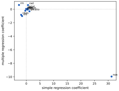
Exercise 15(c). Simple against multiple regression coefficients of each predictor of crim. Code:exercisesin ch03_linear_regression.py. Download: PDF · SVG
Demonstrations for this chapter
Each demonstration runs in the browser on the book's data (or on the simulated data of Figures 3.12 and 3.13, exported by the Python code) and links back to these notes. The ▶ Demo boxes above open them already set to the case under discussion.
| Demonstration | What you can see | Sections |
|---|---|---|
| Confidence and prediction bands on the Advertising data | The least-squares line of sales on TV, radio or newspaper with its standard errors, t, RSE, \(R^2=r^2\) and \(F=t^2\); the confidence band for \(f(x)\) and the prediction band for a new market at any level; twenty new simulated data sets to see what 95% coverage means. Presets: 1 TV; 2 radio; 3 newspaper; 4 far from the mean; 5 20 new data sets. | 3.1.2, 3.1.3, 3.2.2 |
| Leverage and outliers: drag a point | The data of Figures 3.12 and 3.13 with one movable point: fits with and without it, its leverage (3.37), studentized residual and Cook's distance, and the plot of studentized residuals against leverage. Presets: 1 outlier with ordinary \(x\); 2 observation 41; 3 high leverage on the line; 4 leverage \(1/n\); 5 leverage near 1. | 3.3.3 |
| Collinearity and the variance inflation factor | RSS contours of Figure 3.15 for balance on limit with age or with rating, coefficient tables with VIFs, the three-predictor model, and a simulation of the cloud of estimates for any correlation \(\rho\). Presets: 1 age and limit; 2 rating and limit; 3 all three; 4 \(\rho=0\); 5 \(\rho=0.95\). | 3.3.3 |
The Python code for every figure and table is code/ch03_linear_regression.py, and the lab is code/ch03_lab.R and code/ch03_lab.py (see the code index).
References
- James, G., Witten, D., Hastie, T. and Tibshirani, R. (2021). An Introduction to Statistical Learning with Applications in R, 2nd edition. Springer, New York. Chapter 3, pp. 59–128. www.statlearning.com.
- James, G., Witten, D., Hastie, T., Tibshirani, R. and Taylor, J. (2023). An Introduction to Statistical Learning with Applications in Python. Springer, Cham. Chapter 3.
- Hastie, T., Tibshirani, R. and Friedman, J. (2009). The Elements of Statistical Learning: Data Mining, Inference, and Prediction, 2nd edition. Springer, New York. Chapters 2 and 3.
- Belsley, D. A., Kuh, E. and Welsch, R. E. (1980). Regression Diagnostics: Identifying Influential Data and Sources of Collinearity. Wiley, New York.
- Cook, R. D. (1977). Detection of influential observation in linear regression. Technometrics, 19(1), 15–18.
- Harrison, D. and Rubinfeld, D. L. (1978). Hedonic house prices and the demand for clean air. Journal of Environmental Economics and Management, 5(1), 81–102. (The Boston data.)
- Mallows, C. L. (1973). Some comments on Cp. Technometrics, 15(4), 661–675.
- Weisberg, S. (2014). Applied Linear Regression, 4th edition. Wiley, Hoboken.
The numerical statements in the text (every table of the chapter, the derivations' identities, the simulations behind the F-test and the multiple-testing argument, the labs in both languages, the exercise results and the numbers shown by the demonstrations) were confirmed numerically.