Moving Beyond Linearity
A straight line is rarely the truth. This chapter keeps the machinery of least squares but feeds it new columns: powers of the input (polynomials), indicators of intervals (step functions), and piecewise polynomials joined smoothly at knots (regression and natural splines). It then lets a penalty decide how wiggly the curve may be (smoothing splines), fits a separate weighted line around every point (local regression), and adds such curves together, one per input, into a generalised additive model fitted by backfitting. The Wage data run through the chapter, and every figure is recomputed here.
Ch. 1 Introduction Ch. 2 Statistical learning Ch. 3 Linear regression Ch. 4 Classification Ch. 5 Resampling Ch. 6 Selection and regularization Ch. 7 Beyond linearity Ch. 8 Trees Ch. 9 SVMs Ch. 10 Deep learning Ch. 11 Survival analysis Ch. 12 Unsupervised learning Ch. 13 Multiple testing
How to read these notes
They follow the book. Sections carry the book's numbers (7.1, 7.4.3, ...), and displayed equations that appear in the book carry its equation numbers, e.g. \((7.11)\); equations without a number are steps the book skips. Page numbers refer to the R edition (2021); the Python edition (2023) has the same text, figures and exercises a few pages later.
Filling the gaps. Where the book says that a result "can be shown", states it without proof or skips steps, an orange Filling the gap box gives the complete argument at the level of a first course in regression. Derivations start hidden: open one with its bar, or use the button below. Green Deeper lines point to the graduate course on the same authors' larger book.
The lab in two languages. Section 7.8 shows each step in R (left) and Python (right), with the output and the figures. The Python code uses numpy, pandas, scipy and statsmodels only; the spline bases, the smoothing spline, local regression and backfitting are written out as short functions, so nothing is hidden in a package.
Main reference
G. James, D. Witten, T. Hastie and R. Tibshirani, An Introduction to Statistical Learning with Applications in R, 2nd edition, Springer (2021), Chapter 7, pages 289–326, and G. James, D. Witten, T. Hastie, R. Tibshirani and J. Taylor, An Introduction to Statistical Learning with Applications in Python, Springer (2023), Chapter 7 (book website, with the data and the labs: www.statlearning.com). Section, equation, figure and exercise numbers below refer to these books.
The explanations, derivations, figures and code are my own; equations are cited by their numbers in the book.
Companion courses
- Statistical Learning: Theory and Methods (Hastie, Tibshirani and Friedman 2009), the graduate version of this chapter: basis expansions and splines in Chapter 5, local regression in Chapter 6, additive models in Section 9.1. Each section below links to the matching part.
- Bayesian and Probabilistic Machine Learning (Bishop 2006): linear basis function models, the same idea as Section 7.3 seen from the likelihood side.
- Statistical Methods for Modern Biology (Holmes and Huber 2019): loess as used by
geom_smoothand what its band means. - Foundations of Deep Learning (Bishop and Bishop 2024): the basis-function regression demonstration.
The chapter at a glance
- 7.1–7.3 Polynomials, step functions and every other fixed basis \(b_1(X),\dots,b_K(X)\) are linear models in new columns, so least squares, standard errors and F tests carry over. The pointwise standard error of a fitted curve is \(\sqrt{\bl_0^\T\bC\bl_0}\) (Filling the gap 7.1), and it is largest where the data are thin.
- 7.4 A cubic spline with \(K\) knots is a piecewise cubic with two continuous derivatives; it has \(K+4\) degrees of freedom, with the truncated power basis as one basis (Result 7.2). Natural splines are linear beyond the boundary knots and have \(K\) (Result 7.3); that is what tames their boundary variance.
- 7.5 The smoothing spline minimises (7.11) over all functions, and the minimiser is a natural cubic spline with a knot at every distinct \(x_i\) (Result 7.4), shrunk towards a line. Its effective degrees of freedom \(\tr\bS_\lambda\) fall from the number of distinct \(x_i\) to 2 (Result 7.5), and its leave-one-out error needs only one fit (Result 7.6), even with tied \(x_i\).
- 7.6 Local regression fits a weighted line around each target point; it is a linear smoother whose rows are weighted least-squares solutions (Result 7.7).
- 7.7 Additive models add one smooth function per input. With regression splines they are one big least-squares fit; with smoothing splines they are fitted by backfitting (Algorithm 7.2), which converges to the minimiser of a penalised criterion (Result 7.8). Logistic additive models wrap backfitting inside iteratively reweighted least squares (Algorithm 7.3).
Notation. Data \((x_i,y_i)\), \(i=1,\dots,n\). \(\bX\) is the \(n\times p\) model matrix of the basis columns (with a first column of ones), \(\hb=(\bX^\T\bX)^{-1}\bX^\T\by\), \(\hat\sigma^2=\RSS/(n-p)\), and \(\bC=\hat\sigma^2(\bX^\T\bX)^{-1}\) the estimated covariance matrix of \(\hb\). \((u)_+=\max(u,0)\). A linear smoother is a fit of the form \(\hat\by=\bS\by\) with \(\bS\) not depending on \(\by\).
Prerequisites. Least squares and its standard errors (Chapter 3), logistic regression (Chapter 4), cross-validation and the leave-one-out formula (5.2) for least squares (Chapter 5), and ridge regression as a penalised fit (Chapter 6).
p. 289 Linear models are easy to fit, to interpret and to test, but the linearity assumption is almost always an approximation. Chapter 6 improved on least squares by reducing variance (ridge, the lasso, principal components); this chapter instead relaxes linearity, while keeping as much interpretability and as much of the least-squares machinery as possible. Sections 7.1–7.6 model a response \(Y\) as a flexible function of one input \(X\); Section 7.7 combines such functions of several inputs.
7.1 Polynomial Regression
Definition 7.1 (polynomial regression) p. 290, (7.1)
Polynomial regression of degree \(d\) replaces the straight line by
\[ y_i=\beta_0+\beta_1x_i+\beta_2x_i^2+\beta_3x_i^3+\dots+\beta_dx_i^d+\epsilon_i. \tag{7.1} \]It is an ordinary linear model in the \(d\) columns \(x_i,x_i^2,\dots,x_i^d\), fitted by least squares. Degrees above 3 or 4 are rarely useful: the curve becomes very flexible and behaves strangely near the ends of the range of \(X\).
p. 291 On the Wage data (3000 men from the Mid-Atlantic region of the United States, wage in thousands of dollars) the coefficients of a degree-4 fit in age matter less than the fitted curve, which is evaluated on a grid of ages from 18 to 80. Figure 7.1 shows it with a band of two standard errors on either side.
Result 7.1 (the pointwise standard error of a fitted curve) pp. 291–292, (7.2) and footnote 1
At a point \(x_0\) the fit is
\[ \hat f(x_0)=\hat\beta_0+\hat\beta_1x_0+\hat\beta_2x_0^2+\hat\beta_3x_0^3+\hat\beta_4x_0^4=\bl_0^\T\hb,\qquad \bl_0=(1,x_0,x_0^2,x_0^3,x_0^4)^\T. \tag{7.2} \]Its estimated variance is \(\widehat{\Var}\,\hat f(x_0)=\bl_0^\T\bC\bl_0\), with \(\bC=\hat\sigma^2(\bX^\T\bX)^{-1}\) the \(5\times5\) estimated covariance matrix of \(\hb\), and the pointwise standard error is its square root. The band \(\hat f(x_0)\pm2\,\mathrm{SE}\) is an approximate 95% confidence interval for \(f(x_0)\) at each \(x_0\) separately. The same holds for any basis (Section 7.3), with \(\bl_0\) the vector of basis functions at \(x_0\).
Filling the gap 7.1: where \(\bl_0^\T\bC\bl_0\) comes from, why "2 SE" means 95%, and why the logistic band is built on the logit scale pp. 291–292 and p. 315
Derivation
The variance. Write \(\hb=\bA\by\) with \(\bA=(\bX^\T\bX)^{-1}\bX^\T\). If the errors are uncorrelated with variance \(\sigma^2\), then \(\Var(\by)=\sigma^2\bI\) and \(\Var(\hb)=\bA(\sigma^2\bI)\bA^\T=\sigma^2(\bX^\T\bX)^{-1}\). A fixed linear combination \(\bl_0^\T\hb\) has variance \(\bl_0^\T\Var(\hb)\bl_0\), because \(\Var(\ba^\T\bz)=\ba^\T\Var(\bz)\ba\) for any fixed \(\ba\). Replacing \(\sigma^2\) by \(\hat\sigma^2\) gives \(\bl_0^\T\bC\bl_0\). Written out, it is \(\sum_j\sum_k\ell_{0j}\ell_{0k}C_{jk}\): the covariances between the coefficients matter as much as their variances, which is why a table of coefficient standard errors alone cannot give the band.
Why the band opens at the ends. \(\bl_0^\T(\bX^\T\bX)^{-1}\bl_0\) is the leverage a new point at \(x_0\) would have: it is small near the centre of the data and grows quickly where the data are sparse. On the Wage data the degree-4 fit has standard error 1.13 at age 50 but 5.30 at age 18 and 13.63 at age 80 (only 4 men are 80, and few are over 70).
Why 2 SE. If the errors are Gaussian, \(\hat f(x_0)\) is Gaussian with mean \(f(x_0)\) (when the model is right), and \((\hat f(x_0)-f(x_0))/\mathrm{SE}\) has a \(t_{n-p}\) distribution, whose 97.5% point is 1.96 for \(n-p=2995\). So \(\pm2\,\mathrm{SE}\) is a 95.4% interval. It is pointwise: the probability that the whole true curve lies inside the band is lower.
The logistic band (7.3). For logistic regression the same computation applies to the linear predictor \(\hat\eta(x_0)=\bl_0^\T\hb\), with \(\bC=(\bX^\T\hat\bW\bX)^{-1}\) the inverse Fisher information and \(\hat\bW\) diagonal with entries \(\hat p_i(1-\hat p_i)\). The interval \(\hat\eta\pm2\,\mathrm{SE}\) is then mapped through \(p=e^\eta/(1+e^\eta)\). Because this map is increasing, \[ \Pr(a\le\eta\le b)=\Pr\big(\mathrm{expit}(a)\le p\le\mathrm{expit}(b)\big): \] the coverage carries over exactly, and the band stays inside \([0,1]\). A band computed directly on the probability scale (the delta method: \(\mathrm{SE}_p=\hat p(1-\hat p)\,\mathrm{SE}_\eta\)) is symmetric and can go below 0, which is what the lab warns about: at age 80 the logit band of Figure 7.1 is \((1.3\times10^{-14},\,0.73)\), very asymmetric about \(\hat p\).
Confirmed numerically: the hand formula \(\sqrt{\bl_0^\T\bC\bl_0}\) equals the standard errors of R's predict(..., se = TRUE) and of statsmodels' get_prediction to \(10^{-9}\) on the age grid.
Deeper: Statistical Learning: Theory and Methods, Filling the gap 5.4 (the pointwise variance of a least-squares fit) and Filling the gap 5.5 (the standard-error bands of a spline fit).
p. 292 The wages look like a mixture of a large group and a small group of high earners above $250,000. Treating \(I(\text{wage}>250)\) as a binary response, the logistic model
\[ \Pr(y_i>250\given x_i)=\frac{\exp(\beta_0+\beta_1x_i+\beta_2x_i^2+\dots+\beta_dx_i^d)}{1+\exp(\beta_0+\beta_1x_i+\beta_2x_i^2+\dots+\beta_dx_i^d)} \tag{7.3} \]gives the right panel of Figure 7.1. Only 79 of the 3000 men are high earners, so the band is wide, especially beyond age 65.
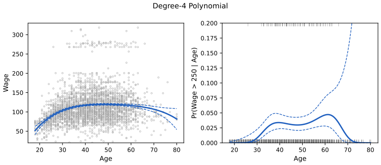
fig_7_1. Reproduces James et al. (2021), Figure 7.1. Download: PDF · SVGFilling the gap 7.2: orthogonal polynomials, and why \(t^2=F\) in the lab pp. 312–315
Derivation
Same fit, different coefficients. R's poly(age, 4) and the raw powers \(\text{age},\dots,\text{age}^4\) (with an intercept) span the same 5-dimensional space of functions. Least squares projects \(\by\) onto the column space of \(\bX\), and the projection depends only on that space, not on the basis chosen for it. So the fitted values agree (the lab finds a largest difference of \(10^{-11}\) in R), while the coefficients and their standard errors are completely different.
How the orthogonal basis is built. poly() applies Gram–Schmidt to \(1,x,x^2,\dots\) on the observed \(x\): with \(p_0=1\), \(p_1=x-a_1\) and \[ p_{k+1}(x)=(x-a_{k+1})p_k(x)-\frac{\|p_k\|^2}{\|p_{k-1}\|^2}p_{k-1}(x),\qquad a_{k+1}=\frac{\sum_ix_ip_k(x_i)^2}{\sum_ip_k(x_i)^2} \] (the three-term recurrence of orthogonal polynomials), each column then scaled to unit length. The \(a_k\) and norms are stored so that the same polynomials can be evaluated at new ages; poly_basis in the Python lab does exactly this and reproduces R's columns.
Why the coefficients do not change with the degree. With orthonormal columns \(\bz_1,\dots,\bz_d\) orthogonal to \(\bone\), \(\bX^\T\bX=\diag(n,1,\dots,1)\), so \(\hat\beta_0=\bar y\) and \(\hat\beta_k=\bz_k^\T\by\): each coefficient is computed on its own, and adding \(\bz_5\) leaves \(\hat\beta_1,\dots,\hat\beta_4\) unchanged (447.068, −478.316, 125.522, −77.911 in both fits of the lab). Their standard errors are all \(\hat\sigma\), because \((\bX^\T\bX)^{-1}\) has ones on the diagonal.
Why \(t^2=F\). Adding \(\bz_k\) to a model that contains \(\bz_1,\dots,\bz_{k-1}\) reduces the RSS by exactly \(\hat\beta_k^2\) (Pythagoras: the new fitted vector differs from the old by \(\hat\beta_k\bz_k\), orthogonal to the old residual's remaining part). R's anova() of several nested models uses \(\hat\sigma^2\) of the largest one, here the degree-5 model, so \(F_k=\hat\beta_k^2/\hat\sigma^2_{(5)}=(\hat\beta_k/\hat\sigma_{(5)})^2=t_k^2\), with \(t_k\) from the degree-5 fit. For the quadratic term, \((-11.983)^2=143.59\). The F test is more general: it works for any nested models, for example with education in the model, where the polynomial columns are no longer orthogonal to the other columns.
7.2 Step Functions
Definition 7.2 (step functions) pp. 292–294, (7.4)–(7.6)
Choose cutpoints \(c_1\lt c_2\lt\dots\lt c_K\) and define the \(K+1\) indicators
\[ C_0(X)=I(X\lt c_1),\ C_1(X)=I(c_1\le X\lt c_2),\ \dots,\ C_{K-1}(X)=I(c_{K-1}\le X\lt c_K),\ C_K(X)=I(c_K\le X). \tag{7.4} \]They sum to 1 for every \(X\), so one of them is dropped when an intercept is present, and the model is
\[ y_i=\beta_0+\beta_1C_1(x_i)+\beta_2C_2(x_i)+\dots+\beta_KC_K(x_i)+\epsilon_i, \tag{7.5} \]or, for a binary response,
\[ \Pr(y_i>250\given x_i)=\frac{\exp(\beta_0+\beta_1C_1(x_i)+\dots+\beta_KC_K(x_i))}{1+\exp(\beta_0+\beta_1C_1(x_i)+\dots+\beta_KC_K(x_i))}. \tag{7.6} \]This turns a continuous input into an ordered categorical one and fits a constant in each bin.
Filling the gap 7.3: the least-squares step function is the bin means p. 293, "\(\beta_0\) can be interpreted as the mean value of \(Y\) for \(X\lt c_1\)"
Derivation
The model (7.5) spans the same functions as \(\sum_{k=0}^K\gamma_kC_k(x)\) (one free constant per bin), with \(\gamma_0=\beta_0\) and \(\gamma_k=\beta_0+\beta_k\). In the \(\gamma\) form the RSS splits into one sum per bin, \(\sum_k\sum_{i\in\text{bin }k}(y_i-\gamma_k)^2\), and each sum is minimised by the bin mean \(\bar y_k\). Hence \(\hat\beta_0=\bar y_0\) and \(\hat\beta_k=\bar y_k-\bar y_0\): each coefficient is the average increase over the first bin. The fitted value in bin \(k\) has standard error \(\hat\sigma/\sqrt{n_k}\), so the band of Figure 7.2 is widest in the last bin, which holds only 72 men. On the Wage data, with R's four equal-width bins (cutpoints 33.5, 49, 64.5), \(\hat\beta=(94.16,\,24.05,\,23.66,\,7.64)\): the mean wage is $94,160 below 33.5 and $118,210 between 33.5 and 49. For the logistic model (7.6) the same argument applied to the log-likelihood shows that the fitted probability in each bin is the proportion of high earners in it.
p. 294 Unless the data have natural breakpoints, steps miss the action: the first bin of Figure 7.2 averages over the steep rise of wage between 18 and 33. Step functions remain popular in epidemiology, where 5-year age groups are standard.
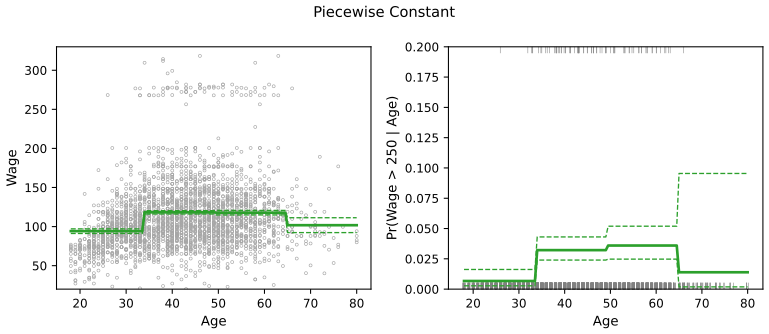
cut(age, 4), cutpoints 33.5, 49 and 64.5). Left: least squares for wage, with \(\pm2\) standard errors. Right: logistic regression for \(\Pr(\text{wage}>250\given\text{age})\). Code: fig_7_2. Reproduces James et al. (2021), Figure 7.2. Download: PDF · SVG7.3 Basis Functions
Definition 7.3 (a basis-function model) p. 294, (7.7)
Fix in advance a family of functions \(b_1(X),\dots,b_K(X)\) and fit
\[ y_i=\beta_0+\beta_1b_1(x_i)+\beta_2b_2(x_i)+\beta_3b_3(x_i)+\dots+\beta_Kb_K(x_i)+\epsilon_i. \tag{7.7} \]Polynomials use \(b_j(x)=x^j\), step functions \(b_j(x)=I(c_j\le x\lt c_{j+1})\); wavelets, Fourier series and splines are other choices. Because the \(b_j\) are known, (7.7) is a linear model in \(K\) derived inputs: least squares, the standard errors of Result 7.1 and the F tests of Chapter 3 all apply unchanged.
Deeper: Statistical Learning: Theory and Methods, Section 5.1 (basis expansions and the three ways of controlling their complexity: restriction, selection and regularisation). See also: linear basis function models in the companion course on probabilistic machine learning.
7.4 Regression Splines
7.4.1 Piecewise Polynomials
p. 295 Instead of one high-degree polynomial over the whole range, fit low-degree polynomials on separate pieces. A piecewise cubic uses
\[ y_i=\beta_0+\beta_1x_i+\beta_2x_i^2+\beta_3x_i^3+\epsilon_i \tag{7.8} \]with coefficients that change at points called knots. With one knot at \(c\), the fit is one cubic on \(\{x_i\lt c\}\) and another on \(\{x_i\ge c\}\), \(2\times4=8\) parameters; with \(K\) knots there are \(K+1\) cubics and \(4(K+1)\) parameters. Step functions are piecewise polynomials of degree 0. Unconstrained, the pieces jump at the knot (Figure 7.3, top left).
7.4.2 Constraints and Splines
Definition 7.4 (spline of degree \(d\)) pp. 296–297
A spline of degree \(d\) with knots \(\xi_1\lt\dots\lt\xi_K\) is a piecewise polynomial of degree \(d\) whose derivatives of order \(0,1,\dots,d-1\) are continuous at every knot. A cubic spline (\(d=3\)) is continuous with continuous first and second derivatives; a linear spline (\(d=1\)) is continuous. Each linear constraint removes one degree of freedom: a cubic spline with one knot has \(8-3=5\), and with \(K\) knots \(4(K+1)-3K=K+4\).
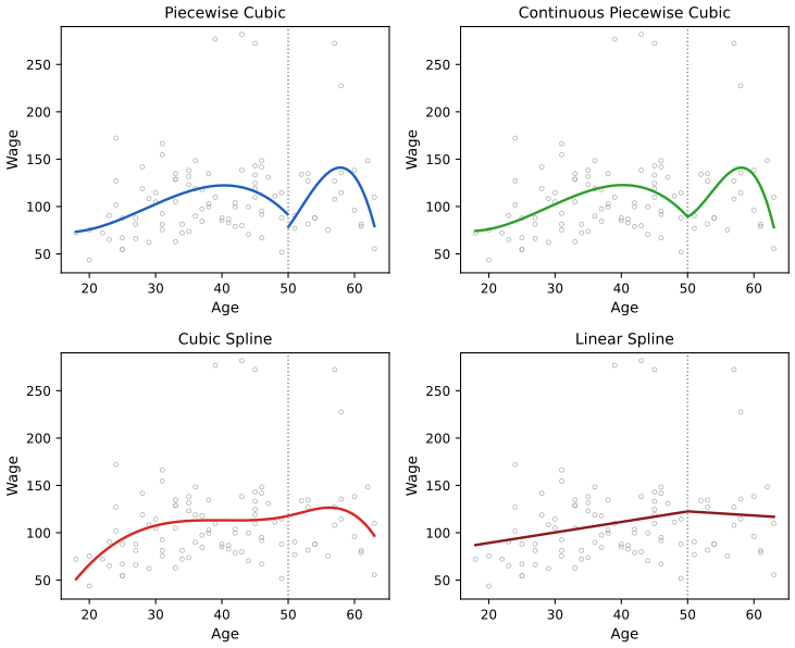
default_rng(7); the book does not say which subset it used. Code: fig_7_3, using the design matrices of truncated_power. Reproduces James et al. (2021), Figure 7.3. Download: PDF · SVG7.4.3 The Spline Basis Representation
p. 297 A cubic spline with \(K\) knots can be written as a basis-function model
\[ y_i=\beta_0+\beta_1b_1(x_i)+\beta_2b_2(x_i)+\dots+\beta_{K+3}b_{K+3}(x_i)+\epsilon_i, \tag{7.9} \]and the most direct choice of basis starts from \(x,x^2,x^3\) and adds one truncated power function per knot,
\[ h(x,\xi)=(x-\xi)_+^3=\begin{cases}(x-\xi)^3 & x>\xi\\ 0 & \text{otherwise.}\end{cases} \tag{7.10} \]Result 7.2 (the truncated power basis of the cubic splines) p. 297, "one can show"; Exercise 1
(a) Adding \(\beta h(x,\xi)\) to a cubic polynomial changes only its third derivative at \(\xi\), by a jump of \(6\beta\); the function and its first two derivatives stay continuous. (b) The \(K+4\) functions \(1,x,x^2,x^3,h(x,\xi_1),\dots,h(x,\xi_K)\) are a basis of the cubic splines with knots \(\xi_1,\dots,\xi_K\): every such spline is a unique combination of them. So fitting a cubic spline is least squares on an intercept and \(K+3\) columns, and uses \(K+4\) degrees of freedom.
Filling the gap 7.4: proof of Result 7.2, and why software uses B-splines instead p. 297
Proof
(a) For \(x\le\xi\), \(h(x,\xi)=0\); for \(x>\xi\), \(h(x,\xi)=(x-\xi)^3\), whose value, first and second derivatives, \(3(x-\xi)^2\) and \(6(x-\xi)\), all tend to 0 as \(x\downarrow\xi\). So \(h\), \(h'\) and \(h''\) are continuous at \(\xi\), and \(h'''\) jumps from 0 to 6. Exercise 1 below does the same computation with explicit coefficients.
(b) They are splines. Each function is a piecewise cubic whose first two derivatives are continuous everywhere, by (a).
They span. Let \(s\) be any cubic spline with these knots, and let \(q_0,\dots,q_K\) be its cubic pieces on the \(K+1\) intervals. At \(\xi_k\) the difference \(q_k-q_{k-1}\) is a cubic that vanishes at \(\xi_k\) with its first two derivatives, so \(q_k(x)-q_{k-1}(x)=c_k(x-\xi_k)^3\) for some \(c_k\) (a cubic with a triple root at \(\xi_k\)). Then \(s(x)=q_0(x)+\sum_kc_kh(x,\xi_k)\) for all \(x\): on the interval after \(\xi_k\) the right side adds up \(q_0+\sum_{j\le k}(q_j-q_{j-1})=q_k\).
They are independent. If \[ a_0+a_1x+a_2x^2+a_3x^3+\sum_kc_kh(x,\xi_k)=0 \] for all \(x\), then to the left of \(\xi_1\) the cubic part vanishes, so \(a_0=\dots=a_3=0\); just to the right of \(\xi_1\) only \(c_1h(x,\xi_1)\) remains, so \(c_1=0\); and so on, knot by knot. Hence the dimension is \(K+4\). The same argument with \((x-\xi)_+^d\) shows that splines of degree \(d\) with \(K\) knots have dimension \(K+d+1\).
B-splines. The truncated powers are badly conditioned: \((x-\xi_k)_+^3\) and \((x-\xi_{k+1})_+^3\) are nearly collinear far to the right of both knots, and they grow like \(x^3\). R's bs() and the Python lab's bs_basis use B-splines instead, a basis of the same space whose functions are non-negative, sum to 1 and are each nonzero on only four knot intervals. The fitted values are identical: the R and Python labs, and the truncated-power fit in the demonstration, agree to rounding error.
Deeper: Statistical Learning: Theory and Methods, Result 5.2 (dimension \(M+K\) for order-\(M\) splines), Filling the gap 5.3 (why the truncated power basis is numerically poor) and Result 5.17 (properties of B-splines).
p. 298 Splines have high variance near the ends of the range of \(X\), where there is little data and the end cubics are free. A remedy is to restrict the ends.
Definition 7.5 (natural cubic spline) p. 298
A natural cubic spline with boundary knots \(\xi_1,\xi_K\) and interior knots \(\xi_2,\dots,\xi_{K-1}\) is a cubic spline on these knots that is linear to the left of \(\xi_1\) and to the right of \(\xi_K\).
Result 7.3 (degrees of freedom of a natural cubic spline) p. 298 and footnote 4, p. 299
Natural cubic splines with \(K\) knots (counting the two boundary knots) form a space of dimension \(K\), constant included. So ns(age, df = 4) (four columns besides the intercept) has \(K=5\) knots: three interior knots, at the quartiles of age, and the two ends of the data.
Filling the gap 7.5: counting the natural spline's degrees of freedom, and why its ends are calmer footnote 4, "somewhat technical"
Derivation
Counting. Treat the \(K\) knots as knots of an ordinary cubic spline: dimension \(K+4\) by Result 7.2. Requiring linearity beyond the boundary knots adds four linear constraints: on the left piece the coefficients of \(x^2\) and \(x^3\) must vanish (equivalently \(f''(\xi_1)=0\) and \(f'''=0\) to the left), and the same on the right. The four constraints are independent (a cubic spline can be found violating any one and satisfying the others), so the dimension is \(K+4-4=K\). Footnote 4 does exactly this count for \(K=5\): \(9-4=5\), one of which is the constant, absorbed by the intercept, which leaves the 4 of df = 4.
A basis. With \(d_k(x)=\frac{(x-\xi_k)_+^3-(x-\xi_K)_+^3}{\xi_K-\xi_k}\), the functions \(N_1=1\), \(N_2=x\), \(N_{k+2}=d_k-d_{K-1}\) for \(k=1,\dots,K-2\) are a basis: beyond \(\xi_K\) the cubic and quadratic terms of each \(d_k\) are the same, \(x^3+(\dots)x^2\) up to the common factor, so they cancel in the differences (ESL (5.4)–(5.5)). The demonstration uses this basis; R's ns() and the lab's ns_basis use an equivalent B-spline construction: start from the cubic B-splines on the knots and keep the combinations whose second derivative is 0 at both boundary knots.
Why the ends are calmer. Near the boundary a cubic spline spends four free parameters on the last piece (a constant, a slope and the two curvature terms), estimated from the few points there; the natural spline spends two. Fewer parameters fitted from the same few points means a smaller variance: on the Wage data, with the same three interior knots, the standard error at age 80 is 8.40 for the natural spline and 14.76 for the cubic spline. The price is a possible bias if the true function curves near the ends.
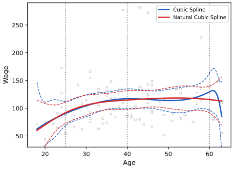
fig_7_4. Reproduces James et al. (2021), Figure 7.4. Download: PDF · SVGDeeper: Statistical Learning: Theory and Methods, Section 5.2.1 and Result 5.3 (natural cubic splines and their basis).
7.4.4 Choosing the Number and Locations of the Knots
pp. 298–300 A spline is most flexible where its knots are dense. In practice knots are usually placed at equally spaced quantiles of the data, and the user chooses only the degrees of freedom: ns(age, df = 4) puts its three interior knots at the 25th, 50th and 75th percentiles (33.75, 42 and 51 years). Figure 7.5 shows that fit for wage and for the probability of a high wage.
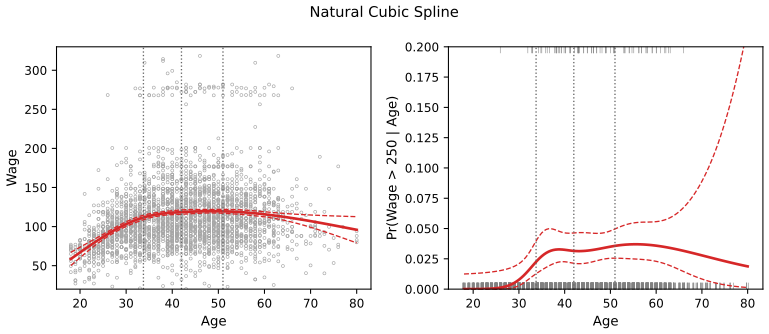
fig_7_5. Reproduces James et al. (2021), Figure 7.5. Download: PDF · SVGHow many degrees of freedom? Ten-fold cross-validation (Chapter 5) estimates the test error for each choice. Figure 7.6 shows it for natural and cubic splines: a straight line (1 df) is clearly inadequate (1675.9), and every fit with three or more df is within about 5 of the best (1593.5 to 1598.6); the curves are flat, so the smallest df on the flat part, 3 or 4, is a sensible choice. When an additive model has several such terms, choosing each df by CV is expensive, and a fixed value such as 4 per term is common.
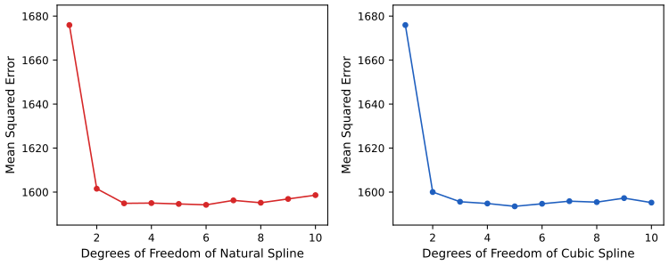
fig_7_6, cv_mse. Reproduces James et al. (2021), Figure 7.6. Download: PDF · SVG7.4.5 Comparison to Polynomial Regression
p. 300 With 15 degrees of freedom, a polynomial must use the power \(x^{15}\), which is huge at the ends of the range, while a natural spline adds knots and keeps the degree at 3. Figure 7.7 shows the consequence: the polynomial swings near age 80 (standard error 19.96 there, against 12.74 for the natural spline), the spline does not. Splines can also put more knots where the function changes quickly.
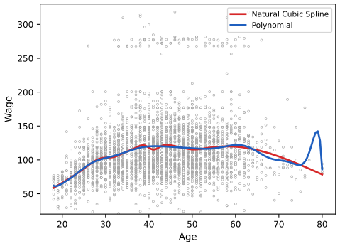
fig_7_7. Reproduces James et al. (2021), Figure 7.7. Download: PDF · SVG7.5 Smoothing Splines
7.5.1 An Overview of Smoothing Splines
p. 301 Minimising the RSS over all functions is pointless (any interpolating \(g\) gives 0). A smoothing spline adds a roughness penalty.
Definition 7.6 (smoothing spline) p. 301, (7.11)
For \(\lambda\ge0\), the smoothing spline is the function \(g\) that minimises
\[ \sum_{i=1}^n\big(y_i-g(x_i)\big)^2+\lambda\int g''(t)^2\,dt. \tag{7.11} \]The first term is a loss, the second a penalty on the total squared curvature, as in ridge regression and the lasso. \(\lambda=0\) allows any interpolant; \(\lambda\to\infty\) forces \(g''=0\), the least-squares line.
Result 7.4 (the minimiser is a shrunken natural cubic spline) p. 302, "can be shown"
Let \(t_1\lt\dots\lt t_m\) be the distinct values among \(x_1,\dots,x_n\) (\(m\ge2\)). For every \(\lambda>0\), (7.11) has a unique minimiser, and it is a natural cubic spline with knots at \(t_1,\dots,t_m\). Writing \(\bg=(g(t_1),\dots,g(t_m))^\T\), \(\bar{\by}\) for the mean response at each \(t_k\) and \(\bW=\diag(w_1,\dots,w_m)\) for the number of observations there,
\[ \hat\bg=(\bW+\lambda\bK)^{-1}\bW\bar{\by}, \]where \(\bK\) is the \(m\times m\) matrix with \(\int g''(t)^2dt=\bg^\T\bK\bg\) for natural cubic splines. It is not the least-squares natural spline with these knots (which interpolates the means): it is that spline shrunk towards the line, more so for larger \(\lambda\).
Filling the gap 7.6: why the minimiser is a natural cubic spline p. 302
Proof
Step 1: interpolation does not increase the penalty. Let \(g\) be any function with a square-integrable second derivative, and let \(\tilde g\) be the natural cubic spline that interpolates \(g\) at \(t_1,\dots,t_m\) (it exists and is unique: \(m\) values determine a natural spline in the \(m\)-dimensional space of Result 7.3). Put \(h=g-\tilde g\), which vanishes at every \(t_k\). Integrate by parts on each interval \([t_k,t_{k+1}]\):
\[ \int_{t_1}^{t_m}\tilde g''h''\,dt=\Big[\tilde g''h'\Big]_{t_1}^{t_m}-\int_{t_1}^{t_m}\tilde g'''h'\,dt=0-\sum_{k=1}^{m-1}\tilde g'''_{(k)}\big(h(t_{k+1})-h(t_k)\big)=0. \]The boundary term is 0 because \(\tilde g''(t_1)=\tilde g''(t_m)=0\) (natural); \(\tilde g'''\) is a constant \(\tilde g'''_{(k)}\) on each interval (a cubic), and \(h\) vanishes at the knots. Hence
\[ \int g''^2=\int(\tilde g''+h'')^2=\int\tilde g''^2+\int h''^2\ \ge\ \int\tilde g''^2, \]with equality only if \(h''=0\) on \([t_1,t_m]\), i.e. \(h\) linear there, hence \(h=0\) (it vanishes at two points or more). Outside \([t_1,t_m]\) the penalty of \(g\) can only be larger; the natural spline is linear there and pays nothing.
Step 2: the minimiser. \(g\) and \(\tilde g\) have the same values at the data, so the same RSS, and \(\tilde g\) has no larger penalty. So a minimiser can be sought among natural cubic splines with knots at the \(t_k\), an \(m\)-dimensional space parametrised by \(\bg\). There the penalty is a quadratic form \(\bg^\T\bK\bg\) (Green and Silverman 1994: \(\bK=\bQ\bR^{-1}\bQ^\T\) with \(\bQ\) and \(\bR\) tridiagonal matrices built from the gaps \(t_{k+1}-t_k\)), and the RSS is \[ \sum_k\sum_{i:x_i=t_k}(y_i-g_k)^2=\text{const}+\sum_kw_k(\bar y_k-g_k)^2. \] Minimising \[ (\bar\by-\bg)^\T\bW(\bar\by-\bg)+\lambda\bg^\T\bK\bg \] gives the normal equations \((\bW+\lambda\bK)\bg=\bW\bar\by\); \(\bW+\lambda\bK\) is positive definite (\(\bK\) is positive semi-definite and \(\bW\) positive definite), so the solution is unique.
Step 3: shrinkage. \(\bK\) has exactly two zero eigenvalues, for the constant and the linear functions (zero curvature). In the basis of the generalised eigenvectors of \((\bK,\bW)\) the fit multiplies the coordinates of \(\bar\by\) by \(1/(1+\lambda d_k)\), with \(0=d_1=d_2\lt d_3\le\dots\le d_m\): the line is kept and the rougher components are shrunk, the roughest most. This is ridge regression on the natural-spline basis, with the curvature as the penalty.
Confirmed numerically: the Reinsch form on the 61 distinct ages (used by the demonstration), a penalised B-spline fit with a knot at every distinct age, and R's smooth.spline(..., all.knots = TRUE) give the same fitted values (to \(10^{-12}\) between the first two, and to \(5\times10^{-6}\) relative with R, whose \(\lambda\) is matched only up to its search tolerance).
Deeper: Statistical Learning: Theory and Methods, Result 5.5 (the smoothing-spline theorem, Exercise 5.7), Result 5.6 (the Reinsch form) and Result 5.7 (the eigenvalues of the smoother).
7.5.2 Choosing the Smoothing Parameter \(\lambda\)
pp. 302–303 The fitted values at the data are linear in \(\by\):
\[ \hat\bg_\lambda=\bS_\lambda\by, \tag{7.12} \]with an \(n\times n\) smoother matrix \(\bS_\lambda\) that depends on the \(x_i\) and \(\lambda\) but not on \(\by\). The effective degrees of freedom are
\[ \df_\lambda=\sum_{i=1}^n\{\bS_\lambda\}_{ii}, \tag{7.13} \]Result 7.5 (effective degrees of freedom) p. 302, "it is possible to show"
(a) \(\df_\lambda=\sum_{k=1}^m\frac{1}{1+\lambda d_k}\) with the \(d_k\) of Filling the gap 7.6; it decreases strictly and continuously from \(m\), the number of distinct \(x_i\), at \(\lambda=0\), to 2 as \(\lambda\to\infty\). The book's "from \(n\) to 2" assumes distinct \(x_i\); for the Wage data \(m=61\), not 3000. (b) For least squares on \(p\) columns, \(\bS=\bH\) is the hat matrix and \(\tr\bH=p\): the definition extends the ordinary count. (c) In general \(\sum_i\Cov(\hat y_i,y_i)=\sigma^2\tr\bS\) when \(\Var(\by)=\sigma^2\bI\), the property that makes \(\tr\bS\) the right count in \(C_p\)-type criteria.
Filling the gap 7.7: the trace of the smoother matrix pp. 302–303
Derivation
(a) Each observation's fitted value is the fitted value at its \(t_k\), which is \(\sum_j\{(\bW+\lambda\bK)^{-1}\bW\}_{kj}\bar y_j\) and \(\bar y_j=\frac1{w_j}\sum_{i:x_i=t_j}y_i\). So for observations \(i\) at \(t_k\) and \(i'\) at \(t_j\), \(\{\bS_\lambda\}_{ii'}=\{(\bW+\lambda\bK)^{-1}\}_{kj}\), and
\[ \tr\bS_\lambda=\sum_kw_k\{(\bW+\lambda\bK)^{-1}\}_{kk}=\tr\big((\bW+\lambda\bK)^{-1}\bW\big)=\tr\bS^{(m)}_\lambda, \]the trace of the \(m\times m\) smoother on the distinct values. Let \(\bK\bu=d\bW\bu\) be the generalised eigenproblem, with \(\bW\)-orthonormal eigenvectors (\(\bU^\T\bW\bU=\bI\)). Then \(\bS^{(m)}_\lambda=\bU\diag\big(\frac1{1+\lambda d_k}\big)\bU^{-1}\), whose trace is \(\sum_k\frac{1}{1+\lambda d_k}\). Each term decreases in \(\lambda\) unless \(d_k=0\); at \(\lambda=0\) all are 1 (sum \(m\)), and as \(\lambda\to\infty\) only the two with \(d_k=0\) survive. So \(\df_\lambda\) can be inverted: R's smooth.spline(df = 16) and the Python lam_for_df find the \(\lambda\) with a given df by a one-dimensional search.
(b) By the cyclic property of the trace,
\[ \tr\bH=\tr\big(\bX(\bX^\T\bX)^{-1}\bX^\T\big)=\tr\big((\bX^\T\bX)^{-1}\bX^\T\bX\big)=\tr\bI_p=p. \](c) \(\Cov(\hat\by,\by)=\Cov(\bS\by,\by)=\bS\sigma^2\), whose diagonal sums to \(\sigma^2\tr\bS\). This covariance is exactly the optimism of the training error (Chapter 5 of the larger book), which is why the effective degrees of freedom of any linear smoother are defined this way.
On the Wage data: \(\df\) runs from 61 to 2. For df = 16, R reports \(\lambda=6.54\times10^{-4}\); R measures age on a \([0,1]\) scale, and on the scale of years this is \(6.54\times10^{-4}\times62^3=155.8\) (with R's subset of 52 knots; 161.0 with a knot at every age).
Result 7.6 (leave-one-out cross-validation from one fit) p. 303, the unnumbered formula
Let \(\hat g^{(-i)}_\lambda\) be the smoothing spline fitted with the same \(\lambda\) to all observations except the \(i\)th. Then
\[ \RSS_{cv}(\lambda)=\sum_{i=1}^n\big(y_i-\hat g^{(-i)}_\lambda(x_i)\big)^2=\sum_{i=1}^n\left[\frac{y_i-\hat g_\lambda(x_i)}{1-\{\bS_\lambda\}_{ii}}\right]^2. \]The identity is exact, and it remains exact when some \(x_i\) are tied, provided \(\{\bS_\lambda\}_{ii}\) is the diagonal of the \(n\times n\) smoother, \(\{(\bW+\lambda\bK)^{-1}\}_{kk}\) for an observation at \(t_k\) (the leverage of its age divided by the number of men of that age). It is the same identity as (5.2) for least squares.
Filling the gap 7.8: proof of the leave-one-out formula, with ties, and generalised cross-validation p. 303 and footnote 5
Proof
The replacement lemma. Fix \(i\) and let \(g^-=\hat g^{(-i)}_\lambda\). Define \(\by^*\) as \(\by\) with \(y_i\) replaced by \(g^-(x_i)\). For any \(g\), the criterion (7.11) with data \(\by^*\) equals the leave-one-out criterion plus \((g^-(x_i)-g(x_i))^2\). The function \(g^-\) minimises the first part and makes the second zero, so it minimises the whole: \(g^-\) is the full-data smoothing spline for the data \(\by^*\). (The space over which we minimise does not change: dropping an observation can only remove a knot, and the minimiser over all functions is the same.)
The formula. By linearity,
\[ g^-(x_i)=\sum_j\{\bS\}_{ij}y_j^*=\hat g(x_i)-\{\bS\}_{ii}y_i+\{\bS\}_{ii}g^-(x_i). \]Solving, \(g^-(x_i)(1-S_{ii})=\hat g(x_i)-S_{ii}y_i\), and subtracting from \(y_i(1-S_{ii})\),
\[ y_i-g^-(x_i)=\frac{y_i-\hat g(x_i)}{1-S_{ii}}. \]Nothing in the argument uses distinct \(x_i\): only that the smoother is a penalised least-squares fit over a space that does not depend on which observations are used. For least squares (\(\lambda=0\) on a fixed basis) it is (5.2).
Ties. With \(w_k\) observations at \(t_k\), \(S_{ii}=\{(\bW+\lambda\bK)^{-1}\}_{kk}\) (Filling the gap 7.7), i.e. the leverage of the age mean divided by \(w_k\). R's smooth.spline(cv = TRUE) warns that "cross-validation with non-unique 'x' values seems doubtful", but its criterion uses exactly this \(S_{ii}\), so it is the exact leave-one-man-out error. The leave-one-out residuals of five men refitted by brute force at df 16 (16.686423, −12.551963, 10.056044, −2.707163, −27.753895) equal the shortcut values to every printed digit.
GCV. Replacing each \(S_{ii}\) by the average \(\df_\lambda/n\) gives generalised cross-validation, \(\mathrm{GCV}(\lambda)=\frac{\RSS(\lambda)/n}{(1-\df_\lambda/n)^2}\), R's default when cv = FALSE.
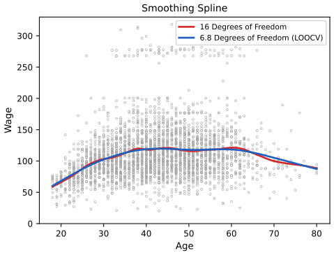
On the Wage data LOOCV is minimised at \(\df=6.82\) (CV error 1593.38 per man); R's search stops at 6.79, the book's 6.8. GCV chooses 6.47. The curve is flat: df 16 has LOOCV error 1597.4.
p. 304 Figure 7.8 compares the fit with 16 df to the LOOCV choice; the two are close, and the simpler one is preferable.
smooth.spline (52 of the 61 distinct ages). Code: fig_7_8, SmoothSpline in the Python lab. Reproduces James et al. (2021), Figure 7.8. Download: PDF · SVGDeeper: Statistical Learning: Theory and Methods, Section 5.4.1 (degrees of freedom and smoother matrices), Filling the gap 5.9 (df is strictly decreasing) and Result 5.9 (leave-one-out from a single fit).
7.6 Local Regression
pp. 304–306 Local regression computes the fit at a target point \(x_0\) from the nearby observations only, with weights that decrease with distance.
Algorithm 7.1 (local regression at \(X=x_0\)) p. 306, (7.14)
- Gather the fraction \(s=k/n\) of training points whose \(x_i\) are closest to \(x_0\).
- Give each of them a weight \(K_{i0}=K(x_i,x_0)\) that is largest for the closest and zero for the farthest; all other points get weight zero.
- Fit a weighted least-squares regression by minimising \[ \sum_{i=1}^nK_{i0}(y_i-\beta_0-\beta_1x_i)^2. \tag{7.14} \]
- The fitted value at \(x_0\) is \(\hat f(x_0)=\hat\beta_0+\hat\beta_1x_0\).
The usual weight is the tricube \(K_{i0}=(1-(|x_i-x_0|/h)^3)^3\) for \(|x_i-x_0|\lt h\), with \(h\) the distance from \(x_0\) to its \(k\)th nearest point, \(k=\lfloor sn\rfloor\). The span \(s\) plays the role of \(\lambda\). A new weighted fit is needed for every \(x_0\): like nearest neighbours, local regression is memory-based.
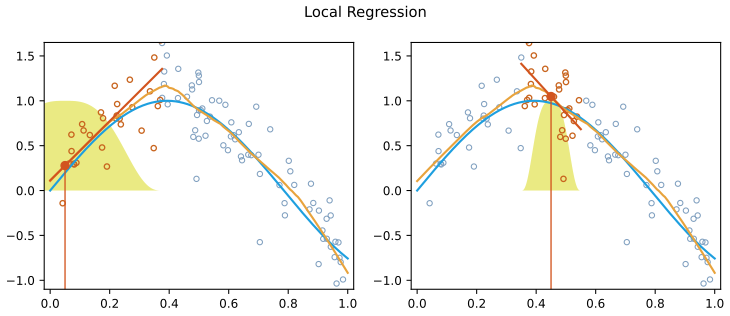
fig_7_9. Reproduces James et al. (2021), Figure 7.9. Download: PDF · SVGResult 7.7 (local regression is a linear smoother) p. 305, "we will avoid getting into the technical details"
With \(\bX_0\) the \(n\times2\) matrix of rows \((1,x_i-x_0)\) and \(\bW_0=\diag(K_{i0})\),
\[ \hat f(x_0)=\be1^\T(\bX_0^\T\bW_0\bX_0)^{-1}\bX_0^\T\bW_0\by=\sum_{i=1}^nl_i(x_0)\,y_i, \]so the fitted values at the data are \(\bS\by\), with row \(i\) of \(\bS\) equal to \((l_1(x_i),\dots,l_n(x_i))\). The weights \(l_i(x_0)\) satisfy \(\sum_il_i(x_0)=1\) and \(\sum_il_i(x_0)(x_i-x_0)=0\): local linear regression reproduces straight lines exactly, at the boundary too, which removes the first-order boundary bias of a local average.
Filling the gap 7.9: the local fit, its degrees of freedom, and what R's loess really fits pp. 305–307, Figure 7.10
Derivation
The formula. Centring the local line at \(x_0\), \(\beta_0+\beta_1(x_i-x_0)\), makes the fitted value at \(x_0\) the intercept. (7.14) is weighted least squares, solved by \(\hb=(\bX_0^\T\bW_0\bX_0)^{-1}\bX_0^\T\bW_0\by\); its first coordinate is \(\hat f(x_0)\). The weights \(l_i(x_0)\) do not depend on \(\by\).
Reproducing lines. If \(y_i=a+b(x_i-x_0)\) exactly, then \(\by=\bX_0(a,b)^\T\) and the weighted fit returns \((a,b)\), so \(\hat f(x_0)=a\). Applying this to \(\by=\bone\) and to \(y_i=x_i-x_0\) gives the two moment conditions. A local constant fit (a weighted average) satisfies only the first; at the left boundary all its neighbours lie to the right, so on a rising curve it is biased upwards by about \(f'(x_0)\) times the mean distance of the neighbours. A local quadratic fit adds the column \((x_i-x_0)^2\) and reproduces parabolas.
Degrees of freedom. As for any linear smoother, \(\df=\tr\bS=\sum_il_i(x_i)\). On the Wage data, local linear fits have \(\tr\bS=10.64\) for span 0.2 and \(3.69\) for span 0.7; local quadratic fits have \(18.28\) and \(5.82\). R's loess reports a different count, the "equivalent number of parameters" \(\tr(\bS^\T\bS)\) (which equals \(\tr\bS\) only for projections), computed on an interpolated approximation of the fit: 16.42 and 5.30 for local quadratic fits. These are the numbers printed in Figure 7.10 (see the notes on the book).
The span with tied \(x\). \(k=\lfloor sn\rfloor\) points are counted with multiplicity: for span 0.2, \(k=600\) men, and \(h\) is the age distance to the 600th nearest man. Men exactly at distance \(h\) get weight 0. The Python loess function computes this directly and agrees with R's loess(..., surface = "direct") to every digit; R's default surface = "interpolate" evaluates the fit exactly at a few vertices and interpolates in between, which changes it by about 0.1 at the ends.
More inputs. In two dimensions the neighbourhood is a disc and the local fit a plane. In \(p\) dimensions a neighbourhood containing a fixed fraction of the data must have a radius close to the whole range once \(p\) exceeds 3 or 4, so the fit stops being local: the same curse of dimensionality as nearest neighbours.
p. 306 Figure 7.10 shows local linear fits to the Wage data with spans 0.2 and 0.7: the larger span gives the smoother curve. Local regression generalises in useful ways: a varying coefficient model is global in some inputs and local in another (time, say), and local fits in two inputs at once are possible; beyond three or four inputs there are too few neighbours.
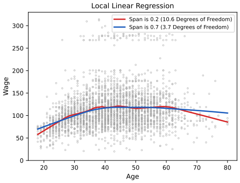
loess with its default local quadratic fits and its "equivalent number of parameters": see the note on Figure 7.10. Code: fig_7_10, loess, loess_trace. Reproduces James et al. (2021), Figure 7.10. Download: PDF · SVGDeeper: Statistical Learning: Theory and Methods, Section 6.1.1 (local linear regression and its equivalent kernel, Result 6.2), Section 6.3 (local regression in \(\R^p\)) and Section 6.4.2 (varying coefficient models). See also: loess as a linear smoother and the meaning of its band in the biology course.
7.7 Generalized Additive Models
p. 306 Generalised additive models (GAMs) extend the multiple linear model by allowing a non-linear function of each input, while keeping the effects additive. They work for quantitative and qualitative responses alike.
7.7.1 GAMs for Regression Problems
Definition 7.7 (additive model) p. 307, (7.15)–(7.16)
Replace each \(\beta_jx_{ij}\) of the linear model by a smooth function \(f_j(x_{ij})\):
\[ y_i=\beta_0+\sum_{j=1}^pf_j(x_{ij})+\epsilon_i=\beta_0+f_1(x_{i1})+f_2(x_{i2})+\dots+f_p(x_{ip})+\epsilon_i. \tag{7.15} \]The functions are identified only up to constants (a constant can move between \(\beta_0\) and any \(f_j\)), so each is centred: \(\sum_if_j(x_{ij})=0\). For the Wage data the model is
\[ \texttt{wage}=\beta_0+f_1(\texttt{year})+f_2(\texttt{age})+f_3(\texttt{education})+\epsilon, \tag{7.16} \]with education a factor with five levels (<HS, HS, <Coll, Coll, >Coll), so \(f_3\) is one constant per level.
pp. 307–308 If each \(f_j\) is a regression spline, (7.16) is one big least-squares fit on the stacked basis columns: here ns(year, 4), ns(age, 5) and four education dummies, RSS 3691918.7 on \(3000-14=2986\) residual df. Figure 7.11 plots each term with its band; the band of a term is \(\sqrt{(\bl_0-\bar\bl)^\T\bC_j(\bl_0-\bar\bl)}\), with \(\bC_j\) the block of \(\bC\) for that term's coefficients and \(\bar\bl\) the average of its basis columns (the centring). Holding the others fixed, wage rises slowly with year (inflation, perhaps), peaks in mid-career, and rises steeply with education.
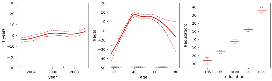
fig_7_11, gam_ns_terms. Reproduces James et al. (2021), Figure 7.11. Download: PDF · SVGp. 309 With smoothing splines as building blocks, least squares no longer applies directly; R's gam() uses backfitting, which updates one term at a time from a partial residual (footnote 6: for \(X_3\), \(r_i=y_i-f_1(x_{i1})-f_2(x_{i2})\)).
Algorithm 7.2 (backfitting) p. 309, described in words; Exercise 11
- Set \(\hat\beta_0=\bar y\) and \(\hat f_j\equiv0\) for every \(j\).
- Cycle over \(j=1,\dots,p,1,\dots,p,\dots\): smooth the partial residual \(r_i=y_i-\hat\beta_0-\sum_{k\ne j}\hat f_k(x_{ik})\) against \(x_{ij}\) with term \(j\)'s smoother \(\bS_j\), and centre the result: \(\hat f_j\leftarrow\bS_j\br-\text{mean}(\bS_j\br)\).
- Stop when no \(\hat f_j\) changes by more than a tolerance.
\(\bS_j\) can be a smoothing spline, a local regression, a straight-line fit, or the level means of a factor; each term uses its own.
Result 7.8 (what backfitting converges to) p. 309
If every \(\bS_j\) is a smoothing spline with penalty \(\lambda_j\) (or a projection, such as a line or a factor), backfitting converges, and its limit minimises
\[ \sum_{i=1}^n\Big(y_i-\beta_0-\sum_jf_j(x_{ij})\Big)^2+\sum_j\lambda_j\int f_j''(t)^2\,dt \]over all centred functions; the minimiser is an additive natural cubic spline. Its effective degrees of freedom are the trace of the overall smoother \(\hat\by=\bS\by\).
Filling the gap 7.10: why backfitting works p. 309, footnote 6
Derivation
The fixed point. Write each term as \(\bf_j=\bN_j\bth_j\) in a natural-spline basis at the data, with penalty \(\lambda_j\bth_j^\T\bOm_j\bth_j\). Setting the gradient of the penalised criterion with respect to \(\bth_j\) to zero gives \[ (\bN_j^\T\bN_j+\lambda_j\bOm_j)\bth_j=\bN_j^\T\Big(\by-\beta_0\bone-\sum_{k\ne j}\bf_k\Big), \] that is \[ \bf_j=\bS_j\Big(\by-\beta_0\bone-\sum_{k\ne j}\bf_k\Big),\qquad \bS_j=\bN_j(\bN_j^\T\bN_j+\lambda_j\bOm_j)^{-1}\bN_j^\T, \] the single-variable smoothing spline. These are the equations backfitting updates one at a time, so any fixed point of backfitting solves the penalised normal equations.
Convergence. Each update of Algorithm 7.2 minimises the penalised criterion exactly over \(\bf_j\) with the other terms held fixed: backfitting is block coordinate descent (the Gauss–Seidel method) on a convex quadratic, so the criterion never increases and the iterates converge to a minimiser. The fitted \(\hat\by\) is unique; the individual \(\bf_j\) are unique once centred, unless two terms can represent the same function (concurvity), for example two identical inputs.
Speed. Convergence is fast when the inputs are nearly unrelated and slow when they are strongly correlated (Exercises 11 and 12). Year, age and education are only weakly related, and one sweep from zero already gets within about 0.5% of the final RSS (3708147 against 3689772 with exact smoothing splines).
Confirmed numerically: the backfitting fit of the Python lab and the direct solution of the penalised normal equations (all terms at once, used for the bands of Figure 7.12) give the same RSS, 3689770.78, and agree with R's gam() (3689770.38) to \(10^{-7}\) relative.
Filling the gap 7.11: counting degrees of freedom, three conventions in one chapter pp. 309, 317–319
smooth.spline(df = 16) counts the constant: \(\tr\bS=16\), and \(\df=2\) is the straight line. In gam(), s(age, 5) does not: the smoother has \(\tr\bS=6\), split into 1 for the linear part and 4 "nonparametric" df, and the constant belongs to \(\beta_0\). ns(age, df = 5) means five columns besides the intercept. So in the lab's model s(year, 4) + s(age, 5) + education the residual df are \(3000-1-4-5-4=2986\), and the book's "four and five degrees of freedom" for Figure 7.12 are counted without constants. The Python edition's approx_lam(..., df = 4 + 1) adds the one for the same reason.
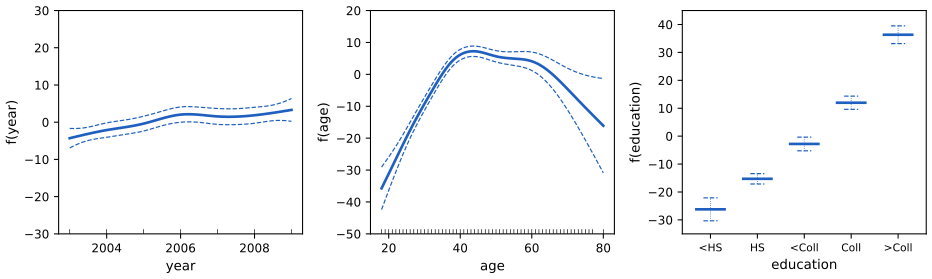
fig_7_12, additive_fit; the backfitting itself is gam_fit in the Python lab. Reproduces James et al. (2021), Figure 7.12. Download: PDF · SVGpp. 309–310 Pros and cons. GAMs fit a non-linear \(f_j\) to each input automatically, which can improve predictions; being additive, each \(f_j\) can be examined with the others held fixed, and its smoothness summarised by its df. The restriction to additivity is the main limitation: interactions are missed unless added by hand, as products \(X_j\times X_k\) or as two-dimensional smooth terms \(f_{jk}(X_j,X_k)\). Fully general models need the methods of Chapter 8.
Deeper: Statistical Learning: Theory and Methods, Section 9.1.1, Algorithm 9.1 (backfitting), Result 9.2 (backfitting is Gauss–Seidel and converges) and Filling the gap 9.3 (degrees of freedom of the whole additive fit).
7.7.2 GAMs for Classification Problems
p. 310 For a binary response with \(p(X)=\Pr(Y=1\given X)\), the logistic model
\[ \log\Big(\frac{p(X)}{1-p(X)}\Big)=\beta_0+\beta_1X_1+\beta_2X_2+\dots+\beta_pX_p \tag{7.17} \]becomes the logistic GAM
\[ \log\Big(\frac{p(X)}{1-p(X)}\Big)=\beta_0+f_1(X_1)+f_2(X_2)+\dots+f_p(X_p). \tag{7.18} \]For the Wage data, with \(p(X)\) the probability that wage exceeds 250 given year, age and education, the book fits
\[ \log\Big(\frac{p(X)}{1-p(X)}\Big)=\beta_0+\beta_1\times\texttt{year}+f_2(\texttt{age})+f_3(\texttt{education}), \tag{7.19} \]with a smoothing spline of 5 df in age and a step function in education.
Algorithm 7.3 (local scoring for a logistic GAM)
- Start from \(\hat\eta_i=\log(\bar y/(1-\bar y))\).
- Compute \(\hat p_i=e^{\hat\eta_i}/(1+e^{\hat\eta_i})\), the weights \(w_i=\hat p_i(1-\hat p_i)\) and the working response \(z_i=\hat\eta_i+(y_i-\hat p_i)/w_i\).
- Fit the additive model to \(z\) by backfitting with weights \(w_i\) (weighted smoothers; R's
gamre-chooses each \(\lambda_j\) so the weighted smoother keeps its df); the result is the new \(\hat\eta\). - Repeat steps 2–3 until the deviance stops changing.
Without the smooth terms this is exactly the iteratively reweighted least squares of logistic regression (Chapter 4).
Filling the gap 7.12: why local scoring works, and why the "<HS" band is enormous pp. 310–311, Figure 7.13
Derivation
Local scoring is Newton's method. For the penalised log-likelihood \(\ell(\eta)-\frac12\sum_j\lambda_j\int f_j''^2\), the Newton step from \(\hat\eta\) solves a penalised weighted least-squares problem with response \(z\) and weights \(w\): the gradient of \(\ell\) in \(\eta_i\) is \(y_i-p_i\) and the negative second derivative is \(p_i(1-p_i)\), so the quadratic approximation of \(\ell\) at \(\hat\eta\) is \(-\frac12\sum_iw_i(z_i-\eta_i)^2+\text{const}\). Step 3 maximises that approximation plus the penalty, and Result 7.8 (with weights) says backfitting solves it.
No high earner has less than a high-school education. The 268 men in "<HS" all have wage \(\le250\). The log-likelihood then keeps increasing as \(f_3(\text{<HS})\to-\infty\): there is no finite maximum (quasi-complete separation for that level). The iterations push the estimate down a little more at each step, while the deviance converges (to 602.459), so the fit stops when the deviance stops changing, at an arbitrary large negative value, and the curvature in that direction is almost zero, so the standard error is huge. In our fit the "<HS" effect is −12.2 with standard error 220, as Figure 7.13 shows. Dropping the 268 men changes nothing for the others (their deviance contribution was 0) and gives the finite, sensible Figure 7.14: the education effects relative to HS are 0.79 (some college), 1.82 (college) and 3.00 (advanced degree) on the logit scale, the same in R and Python to three decimals.
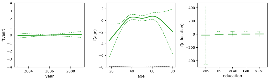
fig_7_13, additive_fit (penalised IRLS). Reproduces James et al. (2021), Figure 7.13. Download: PDF · SVG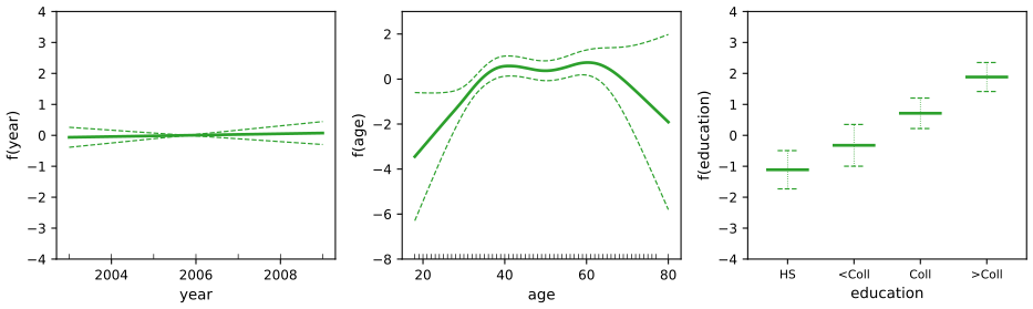
fig_7_14. Reproduces James et al. (2021), Figure 7.14. Download: PDF · SVGDeeper: Statistical Learning: Theory and Methods, Section 9.1.2 and Algorithm 9.2 (local scoring), Result 9.3 (local scoring is Newton–Raphson).
7.8 Lab: Non-linear Modeling
p. 311 The lab re-analyses the Wage data with every method of the chapter. The two editions of the book run the same analyses with different software: the R lab of James et al. 2021 uses lm, glm, splines, smooth.spline, loess and the gam package; the Python lab of James et al. 2023 uses statsmodels with the authors' own helper package and pygam. Here the R version follows the R lab, and the Python version fits the same models as the R version with numpy, pandas, scipy and statsmodels only, writing the bases and smoothers out (see the boxes "The helper functions"). The complete files are code/ch07_lab.R and code/ch07_lab.py; the excerpts below are taken from them verbatim, except that lines which only record a number in cache/ are left out.
Where the two languages differ, and why
- Same numbers. Polynomials, step functions,
bs,ns, the F tests and the local regression fits agree to all printed digits; the GAMs fitted by backfitting agree to \(2\times10^{-7}\) relative; the smoothing spline with 16 df to \(5\times10^{-6}\) (R stops its search for \(\lambda\) at df 16.0024). - Logistic standard errors. R's
glmreports standard errors from the weights of its last-but-one iteration; with the default tolerance they differ from the converged ones in the third digit (26.118 against 26.133 for the first polynomial coefficient). statsmodels, and R with a tighter tolerance, give 26.133, the value printed in the Python edition. - Step functions. R's
cut(age, 4)makes four bins of equal width; the Python edition usespd.qcut, four bins of equal count (cutpoints 33.75, 42, 51), a different model. The Python lab here usespd.cut, to fit R's model. - Local regression. R's
loessfits local quadratics by default (degree = 2); the Python edition uses statsmodels'lowess, which fits local lines and, by default, adds three robustness iterations that down-weight large residuals (at age 40 with span 0.2: 110.32, against 117.88 for a plain local linear fit and 115.37 for R's local quadratic). The Python lab here fits R's model. - Smoothing splines and GAMs. The Python edition fits them with
pygam, a penalised B-spline with 20 basis functions and its own \(\lambda\) scale, so its deviances (3714362, 3696746, 3693143) differ slightly from R's (3711731, 3693842, 3689770). The Python lab here reproduces R's smoothers, including the 52-knot subset thatsmooth.splineuses for 61 distinct ages. - Not in Python.
gam()terms built fromlo()(local regression inside backfitting, and the two-dimensionallo(year, age)) are only in the R lab.
7.8.1 Polynomial Regression and Step Functions
Setup. The data come from the ISLR2 package in R and from the book's CSV file in Python.
R
suppressPackageStartupMessages({
  library(ISLR2)
  library(splines)
  library(gam)
})
options(digits = 6, width = 100)
Python
Wage = common.isl_data("Wage")                      # the 3000 men of the Wage data
y = Wage["wage"].to_numpy()
age = Wage["age"].to_numpy(float)
year = Wage["year"].to_numpy(float)
edu = pd.Categorical(Wage["education"])
E = pd.get_dummies(edu, drop_first=True, dtype=float).to_numpy()   # four dummies, "< HS Grad" is the baseline
n = len(y)
one = np.ones((n, 1))
A degree-4 polynomial. R's poly() builds orthogonal polynomials; poly_basis builds the same columns.
R
fit <- lm(wage ~ poly(age, 4), data = Wage)          # orthogonal polynomial basis
print(coef(summary(fit)))
Python
P4, pc = poly_basis(age, 4)
X = np.column_stack([one, P4])
M = sm.OLS(y, X).fit()
print(pd.DataFrame({"coef": M.params, "std err": M.bse, "t": M.tvalues},
                   index=["intercept"] + ["poly(age, 4)[%d]" % k for k in range(1, 5)]).round(4))
Estimate Std. Error t value Pr(>|t|) (Intercept) 111.7036 0.728741 153.28301 0.00000e+00 poly(age, 4)1 447.0679 39.914785 11.20056 1.48460e-28 poly(age, 4)2 -478.3158 39.914785 -11.98342 2.35583e-32 poly(age, 4)3 125.5217 39.914785 3.14474 1.67862e-03 poly(age, 4)4 -77.9112 39.914785 -1.95194 5.10386e-02
The helper function: poly_basis (Python)
def poly_basis(x, degree, coefs=None):
    """Orthogonal polynomials of degree 1..degree in x (the columns of R's poly(x, degree)).

    The columns are p_1(x), ..., p_d(x) from the three-term recurrence
    p_{k+1}(x) = (x - a_k) p_k(x) - (n_k / n_{k-1}) p_{k-1}(x), scaled to unit length on the
    training data. Pass coefs (returned by the first call) to evaluate the same basis at new x.
    """
    x = np.asarray(x, float)
    if coefs is None:                       # Stieltjes procedure on the training x
        P = [np.ones_like(x)]
        alpha, norm2 = [], [1.0, float(len(x))]
        for k in range(degree):
            a = np.sum(x * P[k] ** 2) / np.sum(P[k] ** 2)
            alpha.append(a)
            nxt = (x - a) * P[k] - (norm2[k + 1] / norm2[k] * P[k - 1] if k > 0 else 0.0)
            P.append(nxt)
            norm2.append(np.sum(nxt ** 2))
        coefs = {"alpha": np.array(alpha), "norm2": np.array(norm2)}
    alpha, norm2 = coefs["alpha"], coefs["norm2"]
    Z = np.ones((len(x), degree + 1))
    Z[:, 1] = x - alpha[0]
    for k in range(1, degree):
        Z[:, k + 1] = (x - alpha[k]) * Z[:, k] - (norm2[k + 1] / norm2[k]) * Z[:, k - 1]
    return Z[:, 1:] / np.sqrt(norm2[2:]), coefs
The raw basis, predictions and standard errors. The raw powers give different coefficients but the same fitted values; the standard error is computed by hand as \(\sqrt{\bl_0^\T\bC\bl_0}\) (Result 7.1) and checked against the built-in one.
R
fit2 <- lm(wage ~ poly(age, 4, raw = TRUE), data = Wage)   # the raw powers age, age^2, age^3, age^4
print(coef(summary(fit2)))
fit2a <- lm(wage ~ age + I(age^2) + I(age^3) + I(age^4), data = Wage)
fit2b <- lm(wage ~ cbind(age, age^2, age^3, age^4), data = Wage)
stopifnot(isTRUE(all.equal(coef(fit2a), coef(fit2b), check.attributes = FALSE)))

agelims <- range(Wage$age)
age.grid <- seq(from = agelims[1], to = agelims[2])
preds <- predict(fit, newdata = list(age = age.grid), se = TRUE)
se.bands <- cbind(preds$fit + 2 * preds$se.fit, preds$fit - 2 * preds$se.fit)
preds2 <- predict(fit2, newdata = list(age = age.grid), se = TRUE)
cat("largest difference between the two bases' fitted values:", max(abs(preds$fit - preds2$fit)), "\n")

# the standard error by hand: Var f(x0) = l0' C l0 with C the covariance matrix of the coefficients
L0 <- cbind(1, poly(age.grid, 4, raw = TRUE))
se.hand <- sqrt(rowSums((L0 %*% vcov(fit2)) * L0))
cat("largest difference between predict()'s and the hand-computed standard errors:",
    max(abs(se.hand - preds2$se.fit)), "\n")
Python
Xraw = np.column_stack([age ** k for k in range(5)])                 # 1, age, ..., age^4
M2 = sm.OLS(y, Xraw).fit()
print("raw-basis coefficients:", np.array2string(M2.params, precision=6))

age_grid = np.arange(age.min(), age.max() + 1)
G = np.column_stack([np.ones(len(age_grid)), poly_basis(age_grid, 4, pc)[0]])
pred = M.get_prediction(G)
fit, se = pred.predicted_mean, pred.se_mean
bands = np.column_stack([fit + 2 * se, fit - 2 * se])
Graw = np.column_stack([age_grid ** k for k in range(5)])
print("largest difference between the two bases' fitted values: %.3g" % np.max(np.abs(fit - Graw @ M2.params)))
se_hand = pointwise_se(Graw, M2.cov_params())                       # sqrt(l0' C l0), Section 7.1
print("largest difference between get_prediction's and the hand-computed standard errors: %.3g" % np.max(np.abs(se_hand - se)))
raw coefficients: -184.154 21.24552 -0.5638593 0.006810688 -0.0000320383 (both languages) R: largest difference between the two bases' fitted values: 1.11e-11; of the standard errors: 4.1e-11 Python: largest difference between the two bases' fitted values: 1.94e-08; of the standard errors: 3.2e-09
The Python difference is larger because statsmodels solves the raw-power fit through a pseudo-inverse of a matrix whose columns range from 1 to \(80^4=4.1\times10^7\); R uses a pivoted QR decomposition. Both are rounding error.
Choosing the degree by nested F tests.
R
fit.1 <- lm(wage ~ age, data = Wage)
fit.2 <- lm(wage ~ poly(age, 2), data = Wage)
fit.3 <- lm(wage ~ poly(age, 3), data = Wage)
fit.4 <- lm(wage ~ poly(age, 4), data = Wage)
fit.5 <- lm(wage ~ poly(age, 5), data = Wage)
av <- anova(fit.1, fit.2, fit.3, fit.4, fit.5)
print(av)
print(coef(summary(fit.5)))
cat("t^2 for the quadratic term:", coef(summary(fit.5))[3, 3]^2, "\n")
Python
fits = [sm.OLS(y, np.column_stack([one, poly_basis(age, d)[0]])).fit() for d in range(1, 6)]
av = anova_lm(*fits)
print(av)
M5 = fits[4]
print("t^2 for the quadratic term: %.3f" % M5.tvalues[2] ** 2)
Res.Df RSS Df Sum of Sq F Pr(>F) 1 2998 5022216 2 2997 4793430 1 228786 143.593 < 2e-16 3 2996 4777674 1 15756 9.889 0.00168 4 2995 4771604 1 6070 3.810 0.05105 5 2994 4770322 1 1283 0.805 0.36968 t^2 for the quadratic term: 143.593
The quadratic and cubic terms are clearly needed, the quartic is borderline (p = 0.051), the fifth power is not (Filling the gap 7.2 explains \(t^2=F\)). With education in the model the F test still works, although the columns are no longer orthogonal:
R
fit.1 <- lm(wage ~ education + age, data = Wage)
fit.2 <- lm(wage ~ education + poly(age, 2), data = Wage)
fit.3 <- lm(wage ~ education + poly(age, 3), data = Wage)
av2 <- anova(fit.1, fit.2, fit.3)
print(av2)
Python
fits_e = [sm.OLS(y, np.column_stack([one, E, poly_basis(age, d)[0]])).fit() for d in range(1, 4)]
av2 = anova_lm(*fits_e)
print(av2)
Res.Df RSS Df Sum of Sq F Pr(>F) 1 2994 3867992 2 2993 3725395 1 142597 114.697 <2e-16 3 2992 3719809 1 5587 4.494 0.0341
Polynomial logistic regression. The band is computed on the logit scale and mapped to probabilities (Filling the gap 7.1).
R
fit <- glm(I(wage > 250) ~ poly(age, 4), data = Wage, family = binomial)
print(coef(summary(fit)))
preds <- predict(fit, newdata = list(age = age.grid), se = TRUE)        # on the logit scale
pfit <- exp(preds$fit) / (1 + exp(preds$fit))
se.bands.logit <- cbind(preds$fit + 2 * preds$se.fit, preds$fit - 2 * preds$se.fit)
se.bands.p <- exp(se.bands.logit) / (1 + exp(se.bands.logit))
Python
high = (y > 250).astype(float)
B = sm.GLM(high, X, family=sm.families.Binomial()).fit()
print(pd.DataFrame({"coef": B.params, "std err": B.bse}).round(4))
eta_hat = G @ B.params
eta_se = pointwise_se(G, B.cov_params())                            # standard errors on the logit scale
pfit = 1 / (1 + np.exp(-eta_hat))
pband = 1 / (1 + np.exp(-np.column_stack([eta_hat + 2 * eta_se, eta_hat - 2 * eta_se])))
coefficients (both): -4.3012 71.9642 -85.7729 34.1626 -47.4008 standard errors, R glm default tolerance: 0.3451 26.1176 35.9043 19.6890 24.0909 standard errors, statsmodels (converged): 0.3453 26.1325 35.9294 19.6967 24.1051
Step functions.
R
print(table(cut(Wage$age, 4)))
fit <- lm(wage ~ cut(age, 4), data = Wage)
print(coef(summary(fit)))
Python
cut_age = pd.cut(age, 4)
print(pd.Series(cut_age).value_counts(sort=False))
S = pd.get_dummies(cut_age, drop_first=True, dtype=float).to_numpy()
Ms = sm.OLS(y, np.column_stack([one, S])).fit()
print("step-function coefficients:", Ms.params.round(4))
(17.9,33.5] (33.5,49] (49,64.5] (64.5,80.1]
750 1399 779 72
coefficients: 94.1584 24.0535 23.6646 7.6406
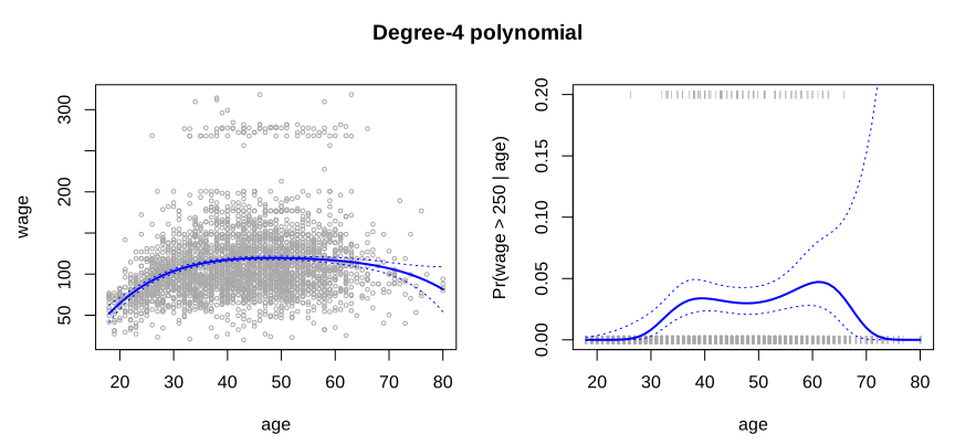
lab-r-poly.svg, made by ch07_lab.R.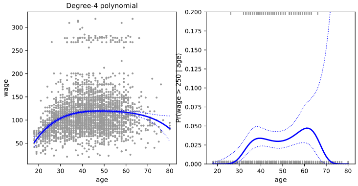
lab-py-poly.svg, made by ch07_lab.py.7.8.2 Splines and Local Regression
Regression splines. A cubic spline with knots at 25, 40 and 60 has six basis columns besides the intercept (\(K+3\)); df = 6 places three knots at the quartiles instead. A natural spline with 4 df has three interior knots.
R
fit <- lm(wage ~ bs(age, knots = c(25, 40, 60)), data = Wage)   # cubic spline, three knots
pred <- predict(fit, newdata = list(age = age.grid), se = TRUE)
print(dim(bs(Wage$age, knots = c(25, 40, 60))))
print(dim(bs(Wage$age, df = 6)))
print(attr(bs(Wage$age, df = 6), "knots"))

fit2 <- lm(wage ~ ns(age, df = 4), data = Wage)                # natural spline, 4 degrees of freedom
pred2 <- predict(fit2, newdata = list(age = age.grid), se = TRUE)
print(attr(ns(Wage$age, df = 4), "knots"))
fit5 <- lm(wage ~ ns(age, df = 5), data = Wage)                # the Python lab's choice
print(coef(summary(fit5)))
Python
Bs, bspec = bs_basis(age, knots=[25, 40, 60])
Mbs = sm.OLS(y, np.column_stack([one, Bs])).fit()
Gbs = np.column_stack([np.ones(len(age_grid)), bs_basis(age_grid, bspec["knots"], boundary=bspec["boundary"])[0]])
pbs = Mbs.get_prediction(Gbs)
print("bs basis:", Bs.shape, "  bs(df=6) knots:", bs_basis(age, df=6)[1]["knots"])

Ns4, nspec = ns_basis(age, df=4)
Mns = sm.OLS(y, np.column_stack([one, Ns4])).fit()
Gns = np.column_stack([np.ones(len(age_grid)), ns_basis(age_grid, nspec["knots"], boundary=nspec["boundary"])[0]])
pns = Mns.get_prediction(Gns)
print("ns(df=4) knots:", nspec["knots"])
Mns5 = sm.OLS(y, np.column_stack([one, ns_basis(age, df=5)[0]])).fit()
print("ns(df=5) coefficients:", Mns5.params.round(4))
[1] 3000 6 bs(age, df = 6) knots: 33.75 42.00 51.00 ns(age, df = 4) knots: 33.75 42.00 51.00 ns(age, df = 5) coefficients: 60.4752 61.5267 55.6912 46.8184 83.2036 6.8770
The helper functions: bs_basis and ns_basis (Python)
def _bspline_design(x, t, k=3, deriv=0):
    """Matrix of all B-splines of degree k with knot vector t (and their derivatives) at x."""
    m = len(t) - k - 1
    out = np.empty((len(np.atleast_1d(x)), m))
    for j in range(m):
        c = np.zeros(m)
        c[j] = 1.0
        b = BSpline(t, c, k, extrapolate=True)
        out[:, j] = b.derivative(deriv)(x) if deriv else b(x)
    return out


def _quantile_knots(x, n_inner):
    """n_inner interior knots at equally spaced quantiles of x (R's default, type 7)."""
    return np.quantile(x, np.linspace(0, 1, n_inner + 2)[1:-1])


def bs_basis(x, knots=None, df=None, degree=3, boundary=None):
    """B-spline basis without the intercept column, as R's bs(x, knots, df, degree)."""
    x = np.asarray(x, float)
    if knots is None:
        knots = _quantile_knots(x, df - degree)
    knots = np.asarray(knots, float)
    lo, hi = boundary if boundary is not None else (x.min(), x.max())
    t = np.r_[[lo] * (degree + 1), knots, [hi] * (degree + 1)]
    B = _bspline_design(x, t, degree)
    spec = {"knots": knots, "boundary": (lo, hi), "degree": degree}
    return B[:, 1:], spec


def ns_basis(x, knots=None, df=None, boundary=None):
    """Natural cubic spline basis without the intercept column, as R's ns(x, knots, df).

    Start from the cubic B-splines on the knots and keep the combinations whose second derivative
    is zero at both boundary knots: those are linear beyond the boundary knots.
    """
    x = np.asarray(x, float)
    if knots is None:
        knots = _quantile_knots(x, df - 1)
    knots = np.asarray(knots, float)
    lo, hi = boundary if boundary is not None else (x.min(), x.max())
    t = np.r_[[lo] * 4, knots, [hi] * 4]
    C = _bspline_design(np.array([lo, hi]), t, 3, deriv=2)[:, 1:]     # 2 x m: f''(lo), f''(hi)
    Q, _ = np.linalg.qr(C.T, mode="complete")                          # last m-2 columns span null(C)
    xin = np.clip(x, lo, hi)
    B = _bspline_design(xin, t, 3)[:, 1:]
    if np.any(x != xin):                                               # beyond the boundary: linear
        D1 = _bspline_design(np.array([lo, hi]), t, 3, deriv=1)[:, 1:]
        B = B + np.where(x < lo, x - lo, 0)[:, None] * D1[0] + np.where(x > hi, x - hi, 0)[:, None] * D1[1]
    spec = {"knots": knots, "boundary": (lo, hi)}
    return B @ Q[:, 2:], spec
Smoothing splines. df = 16 fixes the trace of the smoother; cv = TRUE chooses \(\lambda\) by the leave-one-out shortcut of Result 7.6.
R
fit <- smooth.spline(Wage$age, Wage$wage, df = 16)
fit2 <- suppressWarnings(smooth.spline(Wage$age, Wage$wage, cv = TRUE))   # warns about tied ages
print(fit2$df)
Python
ss = SmoothSpline(age, y)
lam16 = ss.lam_for_df(16)
lam_cv = ss.lam_by_cv()
print("df = 16: lambda = %.4g;  LOOCV: lambda = %.4g, df = %.4f, CV = %.2f" % (lam16, lam_cv, ss.df(lam_cv), ss.loocv(lam_cv)))
R: [1] 6.7946 Python: df = 16: lambda = 0.0006537; LOOCV: lambda = 0.02752, df = 6.8162, CV = 1593.38
R stops its golden-section search over \(\lambda\) a little early: the LOOCV curve is so flat that R's 6.79 df and Python's 6.82 df have the same CV error to seven digits (1593.3835 and 1593.3834).
The helper class: SmoothSpline (Python)
def _nknots_smspl(n):
    """Number of knots R's smooth.spline() uses for n distinct x values."""
    if n < 50:
        return n
    a1, a2, a3, a4 = np.log2(50), np.log2(100), np.log2(140), np.log2(200)
    if n < 200:
        v = 2 ** (a1 + (a2 - a1) * (n - 50) / 150)
    elif n < 800:
        v = 2 ** (a2 + (a3 - a2) * (n - 200) / 600)
    elif n < 3200:
        v = 2 ** (a3 + (a4 - a3) * (n - 800) / 2400)
    else:
        v = 200 + (n - 3200) ** 0.2
    return int(v)


def _penalty_matrix(t, k=3):
    """Omega_jl = integral of B_j''(u) B_l''(u) du, exact (two Gauss points per knot interval)."""
    brk = np.unique(t)
    g = np.array([-1, 1]) / np.sqrt(3)
    mid, half = (brk[1:] + brk[:-1]) / 2, (brk[1:] - brk[:-1]) / 2
    u = (mid[:, None] + half[:, None] * g).ravel()
    w = np.repeat(half, 2)
    D2 = _bspline_design(u, t, k, deriv=2)
    return D2.T @ (w[:, None] * D2)


class SmoothSpline:
    """Cubic smoothing spline: minimise sum_i w_i (y_i - g(x_i))^2 + lam * integral g''(u)^2 du.

    x is rescaled to [0, 1] (as in R, so lam does not depend on the units of x). Ties in x are
    collapsed to their weighted means with summed weights. all_knots=True puts a knot at every
    distinct x, which gives the exact minimiser over all functions (a natural cubic spline);
    otherwise the knots are R's subset (52 of the 61 distinct ages for the Wage data).
    """

    def __init__(self, x, y, w=None, all_knots=False):
        x, y = np.asarray(x, float), np.asarray(y, float)
        w = np.ones_like(x) if w is None else np.asarray(w, float)
        self.ux, inv = np.unique(x, return_inverse=True)
        self.wbar = np.bincount(inv, w)
        self.ybar = np.bincount(inv, w * y) / self.wbar
        self.x, self.y, self.w, self.inv = x, y, w, inv
        self.lo, self.range = self.ux[0], self.ux[-1] - self.ux[0]
        xs = (self.ux - self.lo) / self.range
        nx = len(xs)
        nk = nx if all_knots else _nknots_smspl(nx)
        idx = np.floor(1.0 + np.arange(nk) * ((nx - 1.0) / (nk - 1.0))).astype(int) - 1
        idx[-1] = nx - 1
        self.t = np.r_[[xs[0]] * 3, xs[idx], [xs[-1]] * 3]
        self.B = _bspline_design(xs, self.t)
        self.Omega = _penalty_matrix(self.t)
        self.BtWB = self.B.T @ (self.wbar[:, None] * self.B)
        self.BtWy = self.B.T @ (self.wbar * self.ybar)

    def fit(self, lam):
        """Coefficients, fitted values at the distinct x, and leverages (diagonal of S on distinct x)."""
        A = self.BtWB + lam * self.Omega
        coef = np.linalg.solve(A, self.BtWy)
        Ainv_Bt = np.linalg.solve(A, self.B.T)
        lev = self.wbar * np.einsum("ij,ji->i", self.B, Ainv_Bt)
        return coef, self.B @ coef, lev

    def df(self, lam):
        """Effective degrees of freedom tr(S_lam) (7.13); between 2 and the number of distinct x."""
        return self.fit(lam)[2].sum()

    def lam_for_df(self, df):
        """The lam with df(lam) = df: df is strictly decreasing in lam, so a root search works."""
        f = lambda s: self.df(10.0 ** s) - df
        lo = -12.0
        while not np.isfinite(f(lo)) or f(lo) < 0:      # very small lam can be numerically singular
            lo += 1.0
        return 10.0 ** optimize.brentq(f, lo, 6, xtol=1e-12)

    def loocv(self, lam):
        """Leave-one-out CV error per observation from one fit: the shortcut formula of Section 7.5.2."""
        _, g, lev = self.fit(lam)
        s_ii = lev / self.wbar                  # diagonal of the n x n smoother matrix, observation by observation
        r = (self.y - g[self.inv]) / (1 - s_ii[self.inv])
        return np.average(r ** 2, weights=self.w)

    def lam_by_cv(self, grid=np.linspace(-8, 2, 201)):
        cv = np.array([self.loocv(10.0 ** s) for s in grid])
        k = int(np.argmin(cv))
        res = optimize.minimize_scalar(lambda s: self.loocv(10.0 ** s), bounds=(grid[max(k - 1, 0)], grid[min(k + 1, len(grid) - 1)]),
                                       method="bounded", options={"xatol": 1e-9})
        return 10.0 ** res.x

    def predict(self, lam, xnew, coef=None):
        """g at new x; beyond the data range the natural spline continues as a straight line."""
        coef = self.fit(lam)[0] if coef is None else coef
        xs = (np.asarray(xnew, float) - self.lo) / self.range
        xin = np.clip(xs, 0, 1)
        g = _bspline_design(xin, self.t) @ coef
        if np.any(xs != xin):
            d1 = _bspline_design(np.array([0.0, 1.0]), self.t, deriv=1) @ coef
            g = g + np.where(xs < 0, xs, 0) * d1[0] + np.where(xs > 1, xs - 1, 0) * d1[1]
        return g
Local regression.
R
fit <- loess(wage ~ age, span = .2, data = Wage)
fit2 <- loess(wage ~ age, span = .5, data = Wage)
Python
lo2, lo5 = loess(age, y, age_grid, 0.2), loess(age, y, age_grid, 0.5)fits at ages 20, 40, 60, 80 (span 0.2, local quadratic, exact): 66.2049 115.3742 120.8408 84.4642 (both)
The helper function: loess (Python)
def loess(x, y, xnew, span, degree=2, w=None):
    """Local polynomial regression (Algorithm 7.1 with a local polynomial of the given degree).

    At each target x0: take the q = floor(span * n) nearest x_i, give them tricube weights
    (1 - (d / d_q)^3)^3 where d_q is the distance to the q-th nearest, and fit weighted least squares.
    """
    x, y = np.asarray(x, float), np.asarray(y, float)
    w = np.ones_like(x) if w is None else np.asarray(w, float)
    q = int(np.floor(span * len(x)))
    out = np.empty(len(np.atleast_1d(xnew)))
    for i, x0 in enumerate(np.atleast_1d(xnew)):
        d = np.abs(x - x0)
        h = np.partition(d, q - 1)[q - 1]
        k = w * np.clip(1 - (d / h) ** 3, 0, None) ** 3
        X = np.vander(x - x0, degree + 1, increasing=True)
        sw = np.sqrt(k)
        beta = np.linalg.lstsq(X * sw[:, None], y * sw, rcond=None)[0]
        out[i] = beta[0]                        # the fitted value at x0 is the local intercept
    return out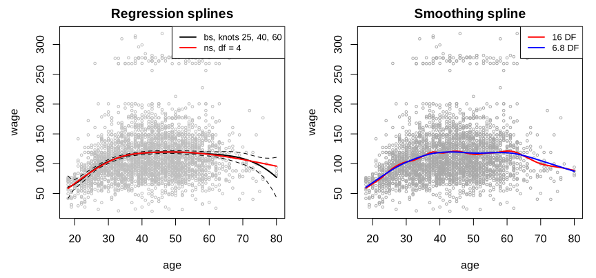
lab-r-splines.svg.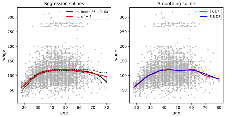
lab-py-splines.svg.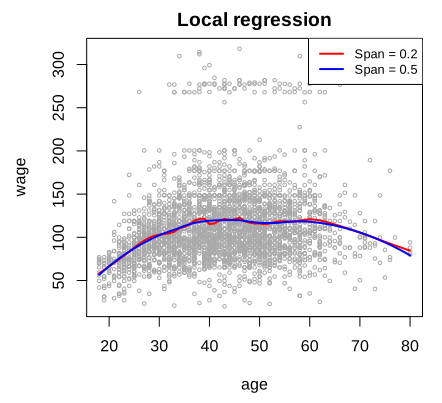
lab-r-loess.svg.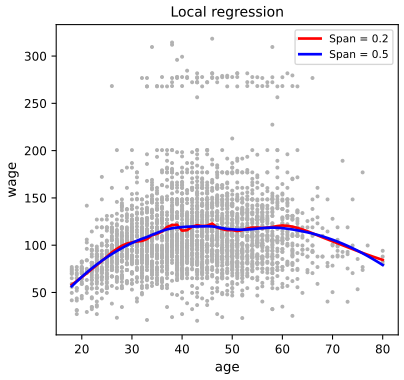
lab-py-loess.svg.7.8.3 GAMs
Natural splines: one least-squares fit.
R
gam1 <- lm(wage ~ ns(year, 4) + ns(age, 5) + education, data = Wage) # natural splines: plain least squaresPython
Nyear = ns_basis(year, df=4)[0]
Nage = ns_basis(age, df=5)[0]
gam1 = sm.OLS(y, np.column_stack([one, Nyear, Nage, E])).fit()      # natural splines: one least-squares fit
print("GAM with natural splines: RSS = %.1f" % gam1.ssr)
RSS = 3691918.7 (both)
Smoothing splines by backfitting, and F tests between three nested GAMs: no year (M1), linear in year (M2), a spline in year (M3).
R
gam.m3 <- gam(wage ~ s(year, 4) + s(age, 5) + education, data = Wage)    # smoothing splines: backfitting
gam.m1 <- gam(wage ~ s(age, 5) + education, data = Wage)
gam.m2 <- gam(wage ~ year + s(age, 5) + education, data = Wage)
av3 <- anova(gam.m1, gam.m2, gam.m3, test = "F")
print(av3)
print(summary(gam.m3))
Python
lin = lambda M_: {"type": "linear", "X": M_}
m3 = gam_fit(y, [{"type": "smooth", "x": year, "df": 4}, {"type": "smooth", "x": age, "df": 5}, lin(E)])
m2 = gam_fit(y, [lin(year[:, None]), {"type": "smooth", "x": age, "df": 5}, lin(E)])
m1 = gam_fit(y, [{"type": "smooth", "x": age, "df": 5}, lin(E)])
dev = np.array([m1["deviance"], m2["deviance"], m3["deviance"]])
resdf = np.array([n - 1 - 5 - 4, n - 1 - 1 - 5 - 4, n - 1 - 4 - 5 - 4])
disp = dev[2] / resdf[2]                                             # dispersion of the largest model
F = -np.diff(dev) / -np.diff(resdf) / disp
p = stats.f.sf(F, -np.diff(resdf), resdf[2])
print(pd.DataFrame({"Resid. Df": resdf, "Resid. Dev": dev.round(1), "F": np.r_[np.nan, F], "Pr(>F)": np.r_[np.nan, p]}))
Resid. Df Resid. Dev Df Deviance F Pr(>F) 1 2990 3711731 (Python: 3711730.1) 2 2989 3693842 1 17889 14.477 0.000145 (Python: 3693840.7, F 14.477, p 0.000145) 3 2986 3689770 3 4071 1.098 0.348566 (Python: 3689770.8, F 1.098, p 0.3487)
A linear trend in year is needed (p = 0.00014); a non-linear one is not (p = 0.35). R's summary also prints "Anova for Nonparametric Effects", an approximate test of each smooth term against its linear part: \(F=1.09\) on 3 df for year and \(F=32.4\) on 4 df for age. Refitting with each term made linear gives exact F tests with the same conclusion (\(F=1.10\) and \(F=32.3\), in the backfitting demonstration).
The helper function: gam_fit, backfitting and local scoring (Python)
def _wls_projection(X, w):
    """The weighted least-squares fit on [1, X] as a function: r -> X1 (X1'WX1)^{-1} X1'W r.

    The constant column makes the block reproduce constants, as a smoothing spline does; the fitted
    term is then centred, and the intercept is carried by alpha.
    """
    X = np.column_stack([np.ones(len(X)), X])
    XtW = (X * w[:, None]).T
    M = np.linalg.solve(XtW @ X, XtW)
    return lambda r: X @ (M @ r)


def gam_fit(y, terms, family="gaussian", tol=1e-10, maxit=200):
    """Additive model y ~ alpha + sum_j f_j by backfitting; logistic models by local scoring.

    terms: list of dicts, each either {"type": "linear", "X": matrix} (a parametric block, fitted
    by least squares on the partial residual) or {"type": "smooth", "x": x, "df": df} (a smoothing
    spline with tr(S) = df + 1, the convention of gam::s()). Returns the intercept, the fitted
    term contributions (each centred to weighted mean 0), the linear predictor and the deviance.
    """
    y = np.asarray(y, float)
    n = len(y)
    eta = np.zeros(n)
    if family == "binomial":
        p0 = y.mean()
        eta[:] = np.log(p0 / (1 - p0))
    fs = [np.zeros(n) for _ in terms]
    alpha = eta.mean()
    for outer in range(100):
        if family == "binomial":                # local scoring: working response and weights
            mu = 1 / (1 + np.exp(-eta))
            w = np.maximum(mu * (1 - mu), 1e-10)
            z = eta + (y - mu) / w
        else:
            w, z = np.ones(n), y
        smoothers, makers = [], []
        for term in terms:
            if term["type"] == "linear":
                smoothers.append(_wls_projection(term["X"], w))
                X1 = np.column_stack([np.ones(n), term["X"]])
                makers.append(lambda r, X1=X1: ("linear", np.linalg.lstsq(X1 * np.sqrt(w)[:, None], r * np.sqrt(w), rcond=None)[0]))
            else:
                ss = SmoothSpline(term["x"], np.zeros(n), w=w, all_knots=term.get("all_knots", False))
                lam = ss.lam_for_df(term["df"] + 1)
                A = np.linalg.solve(ss.BtWB + lam * ss.Omega, ss.B.T)
                def smooth(r, ss=ss, A=A):
                    rbar = np.bincount(ss.inv, ss.w * r) / ss.wbar
                    return (ss.B @ (A @ (ss.wbar * rbar)))[ss.inv]
                smoothers.append(smooth)
                makers.append(lambda r, ss=ss, A=A, lam=lam: ("smooth", ss, A @ (ss.wbar * np.bincount(ss.inv, ss.w * r) / ss.wbar), lam))
        alpha = np.average(z - sum(fs), weights=w)
        for it in range(maxit):                  # backfitting (Algorithm in Section 7.7)
            change = 0.0
            for j, S in enumerate(smoothers):
                partial = z - alpha - sum(fs[k] for k in range(len(fs)) if k != j)
                new = S(partial)
                new -= np.average(new, weights=w)
                change = max(change, np.max(np.abs(new - fs[j])))
                fs[j] = new
            alpha = np.average(z - sum(fs), weights=w)
            if change < tol * (1 + np.max(np.abs(z))):
                break
        eta_new = alpha + sum(fs)
        if family == "gaussian":
            eta = eta_new
            break
        conv = np.max(np.abs(eta_new - eta)) < 1e-9
        eta = eta_new
        if conv:
            break
    if family == "gaussian":
        dev = np.sum((y - eta) ** 2)
    else:
        mu = 1 / (1 + np.exp(-eta))
        dev = -2 * np.sum(y * np.log(np.clip(mu, 1e-300, 1)) + (1 - y) * np.log(np.clip(1 - mu, 1e-300, 1)))
    # the fitted term functions, for prediction at new inputs: f_j = (smoother applied to its partial
    # residual) minus its weighted mean
    parts = []
    for j, mk in enumerate(makers):
        partial = z - alpha - sum(fs[k] for k in range(len(fs)) if k != j)
        made = mk(partial)
        shift = np.average(smoothers[j](partial), weights=w)
        parts.append(made + (shift,))
    return {"alpha": alpha, "f": fs, "eta": eta, "deviance": dev, "parts": parts}


def gam_predict(fit, new_terms):
    """Linear predictor at new data; new_terms lists, term by term, the new x (smooth) or X (linear)."""
    eta = fit["alpha"]
    for part, new in zip(fit["parts"], new_terms):
        if part[0] == "linear":
            beta, shift = part[1], part[2]
            eta = eta + np.column_stack([np.ones(len(new)), new]) @ beta - shift
        else:
            ss, coef, lam, shift = part[1], part[2], part[3], part[4]
            eta = eta + ss.predict(lam, new, coef=coef) - shift
    return eta
Local regression terms (R only): gam(wage ~ s(year, df = 4) + lo(age, span = 0.7) + education) has deviance 3716672, and the two-dimensional lo(year, age, span = 0.5) term 3688928. R warns that a workspace of the underlying loess code is too small for the two-dimensional term; the lab suppresses the warning.
A logistic GAM. Nobody in "<HS" earns more than $250,000, so that level is dropped (Filling the gap 7.12):
R
gam.lr <- gam(I(wage > 250) ~ year + s(age, df = 5) + education, family = binomial, data = Wage)
print(table(Wage$education, I(Wage$wage > 250)))
gam.lr.s <- gam(I(wage > 250) ~ year + s(age, df = 5) + education, family = binomial,
                data = Wage, subset = (education != "1. < HS Grad"))
Python
print(pd.crosstab(Wage["education"], y > 250))
keep_rows = edu.codes != 0
E_s = pd.get_dummies(pd.Categorical(Wage["education"][keep_rows]), drop_first=True, dtype=float).to_numpy()
lr_s = gam_fit(high[keep_rows], [lin(year[keep_rows, None]), {"type": "smooth", "x": age[keep_rows], "df": 5}, lin(E_s)],
               family="binomial")
print("logistic GAM without < HS Grad: deviance = %.3f" % lr_s["deviance"])
FALSE TRUE 1. < HS Grad 268 0 2. HS Grad 966 5 3. Some College 643 7 4. College Grad 663 22 5. Advanced Degree 381 45 deviance without <HS: R 602.4588, Python 602.4587; education effects 0.7882, 1.8236, 2.9968 (both)
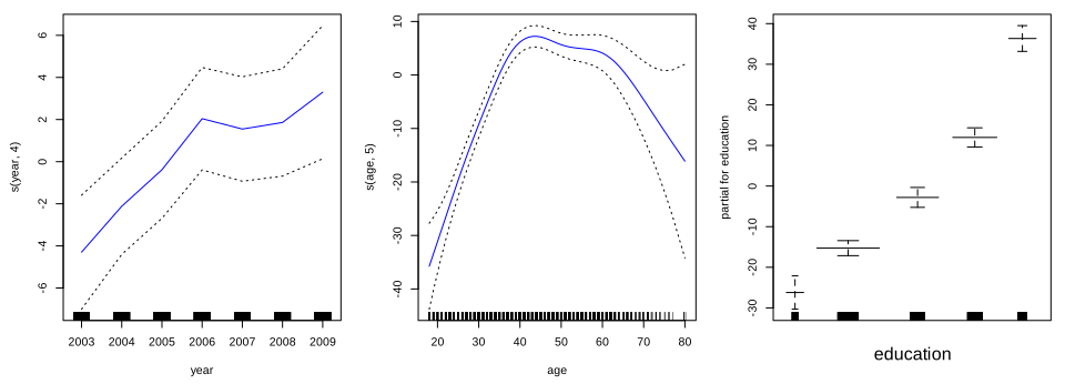
plot(gam.m3, se = TRUE), lab-r-gam.svg.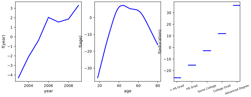
lab-py-gam.svg (bands in Figure 7.12).Notes on the book
Figure 7.10 and the R lab: the "local linear" fits are local quadratic
Section 7.6 describes local linear regression, Figure 7.10 is titled "Local Linear Regression", and the R lab (p. 318) says "Here we have performed local linear regression using spans of 0.2 and 0.5". But R's loess() fits local quadratics unless degree = 1 is given. The legend of Figure 7.10 confirms it: R reports an "equivalent number of parameters" of 16.42 for loess(wage ~ age, span = 0.2) and 5.30 for span 0.7 (the book's 16.4 and 5.3), but 9.02 and 3.31 with degree = 1. Moreover this number is \(\tr(\bS^\T\bS)\), not the \(\tr\bS\) of (7.13): the local linear smoothers have \(\tr\bS=10.6\) and 3.7, which is what our Figure 7.10 prints.
The Python lab's local regression is robust local linear regression
The Python lab (Section 7.8.4 of the 2023 edition) fits sm.nonparametric.lowess(y, age, frac=span), described as local linear regression. statsmodels' lowess runs three robustness iterations by default (it=3), which down-weight observations with large residuals; on the Wage data, whose high earners are large residuals, this lowers the curve (110.3 at age 40 with span 0.2, against 117.9 for plain local linear regression). Pass it=0 for the method of Algorithm 7.1.
The Python lab's F tests with education treat education as a number
Out[11] of the Python lab (residual df 2997, 2996, 2995; RSS 3.902, 3.759, 3.754 million; F = 113.992 and 4.729) is reproduced exactly when education enters as a single numeric column with values 1 to 5. With education as a five-level factor, as in the R lab, the residual df are 2994, 2993, 2992, the RSS 3.868, 3.725, 3.720 million, and F = 114.70 and 4.49. The text's "a linear term in education" describes the numeric version; the two editions fit different models here.
The Python lab swaps the degrees of freedom of year and age
Model (7.16) and Figure 7.11 use natural splines with 4 df for year and 5 for age (the R lab: ns(year, 4) + ns(age, 5)). In[28] of the Python lab uses NaturalSpline(df=4) for age and df=5 for year. Both have 2986 residual df, but they are different models: RSS 3695815 against 3691919.
A typo in the Python lab's step-function check
After In[20] the Python lab writes "94.158 + 22.349 = 116.507 \(\approx\) 116.611, the latter being the mean in the second bin in cell [15]". Cell [15] prints 116.6608, and the second bin's mean is 116.6608. The explanation of the difference (qcut puts ages equal to a cutpoint in the lower bin, bs(degree=0) in the upper one) is right.
Exercise 11 in the Python edition refers to the wrong parts
The Python edition inserts a new part (b) (write simple_reg()), which shifts the later parts by one letter, but part (f) still says "Write a for loop to repeat (c) and (d) 1,000 times" (it should be (d) and (e)), and part (g) "Compare your answer in (e)" (it should be (f)).
"From \(n\) to 2" needs distinct inputs
Section 7.5.2 says that \(\df_\lambda\) decreases from \(n\) to 2. That holds when the \(x_i\) are distinct. With ties the smoother has rank at most the number \(m\) of distinct values, and \(\df_\lambda\) decreases from \(m\) to 2 (Result 7.5): for the Wage data from 61, not 3000.
Exercises
Conceptual exercises 1–5 and applied exercises 6–12, in the book's numbering (the two editions have the same exercises; Exercise 11 has one extra part in the Python edition). The applied solutions are the last sections of ch07_lab.R and ch07_lab.py. Cross-validation folds are fixed by row number (row \(i\) in fold \(i\bmod10\)), and the toy data of Exercises 11 and 12 are deterministic, so that both languages give the same numbers.
Exercise 7.1. Show that \[ f(x)=\beta_0+\beta_1x+\beta_2x^2+\beta_3x^3+\beta_4(x-\xi)_+^3 \] is a cubic spline with a knot at \(\xi\) for any coefficients: (a) find the cubic \(f_1\) equal to \(f\) for \(x\le\xi\); (b) the cubic \(f_2\) equal to \(f\) for \(x>\xi\); (c)–(e) show that \(f_1\) and \(f_2\) agree at \(\xi\) with their first and second derivatives.
Solution
(a) For \(x\le\xi\) the truncated term is 0: \(a_1=\beta_0,\ b_1=\beta_1,\ c_1=\beta_2,\ d_1=\beta_3\).
(b) For \(x>\xi\), \((x-\xi)^3=x^3-3\xi x^2+3\xi^2x-\xi^3\), so \(a_2=\beta_0-\beta_4\xi^3\), \(b_2=\beta_1+3\beta_4\xi^2\), \(c_2=\beta_2-3\beta_4\xi\), \(d_2=\beta_3+\beta_4\).
(c)
\[ f_2(\xi)-f_1(\xi)=\beta_4(-\xi^3+3\xi^3-3\xi^3+\xi^3)=0. \](d)
\[ f_2'(\xi)-f_1'(\xi)=(b_2-b_1)+2(c_2-c_1)\xi+3(d_2-d_1)\xi^2=\beta_4(3\xi^2-6\xi^2+3\xi^2)=0. \](e)
\[ f_2''(\xi)-f_1''(\xi)=2(c_2-c_1)+6(d_2-d_1)\xi=\beta_4(-6\xi+6\xi)=0. \]Only the third derivative jumps, by \(6(d_2-d_1)=6\beta_4\): Result 7.2(a). Checked numerically for random coefficients.
Exercise 7.2. Sketch \[ \hat g=\argmin_g\Big(\sum_i(y_i-g(x_i))^2+\lambda\int[g^{(m)}(x)]^2dx\Big) \] for (a) \(\lambda=\infty,m=0\); (b) \(\lambda=\infty,m=1\); (c) \(\lambda=\infty,m=2\); (d) \(\lambda=\infty,m=3\); (e) \(\lambda=0,m=3\).
Solution
As \(\lambda\to\infty\) the penalty must vanish, \(g^{(m)}\equiv0\), and among such functions the RSS is minimised. (a) \(g\equiv0\): the horizontal axis. (b) \(g'\equiv0\): a constant, the least-squares one, \(\hat g\equiv\bar y\). (c) \(g''\equiv0\): the least-squares line. (d) \(g'''\equiv0\): the least-squares quadratic. (e) With \(\lambda=0\) only the RSS counts, and any function through all the points (one value per distinct \(x\), the mean there if \(x\) is tied) is a minimiser; the limit of \(\hat g\) as \(\lambda\downarrow0\) is the smoothest interpolant, a natural spline of degree \(2m-1=5\) through the points, which wiggles wildly. On the Wage data the limits (b)–(d) are the constant 111.70 and the degree-1 and degree-2 polynomials of the lab.
Exercise 7.3. With \(b_1(X)=X\), \(b_2(X)=(X-1)^2I(X\ge1)\) and \(\hat\beta_0=1,\hat\beta_1=1,\hat\beta_2=-2\), sketch the curve on \([-2,2]\).
Solution
\(\hat f(X)=1+X\) for \(X\lt1\): a line with intercept 1 and slope 1, from \(-1\) at \(X=-2\) to 2 at \(X=1\). For \(X\ge1\), \(\hat f(X)=1+X-2(X-1)^2\), a downward parabola: value 2 and slope \(1-4(X-1)=1\) at \(X=1\) (so \(\hat f\) and \(\hat f'\) are continuous; \(\hat f''\) jumps from 0 to \(-4\)), maximum \(2.125\) at \(X=1.25\), and \(\hat f(2)=1\). The intercept on the vertical axis is \(\hat f(0)=1\).
Exercise 7.4. With \[ b_1(X)=I(0\le X\le2)-(X-1)I(1\le X\le2),\quad b_2(X)=(X-3)I(3\le X\le4)+I(4\lt X\le5) \] and \(\hat\beta_0=1,\hat\beta_1=1,\hat\beta_2=3\), sketch the curve on \([-2,6]\).
Solution
\(\hat f=1+b_1+3b_2\), piece by piece: \(1\) on \([-2,0)\); \(2\) on \([0,1)\); \(3-X\) on \([1,2]\), falling from 2 to 1; \(1\) on \((2,3)\); \(1+3(X-3)\) on \([3,4]\), rising from 1 to 4; \(4\) on \((4,5]\); \(1\) on \((5,6]\). The curve jumps up at \(X=0\) and down at \(X=5\), and is continuous elsewhere; the intercept is \(\hat f(0)=2\).
Exercise 7.5. \(\hat g_1\) and \(\hat g_2\) penalise \(\int[g^{(3)}]^2\) and \(\int[g^{(4)}]^2\) respectively. (a) As \(\lambda\to\infty\), which has the smaller training RSS? (b) The smaller test RSS? (c) For \(\lambda=0\)?
Solution
(a) In the limit \(\hat g_1\) is the least-squares quadratic and \(\hat g_2\) the least-squares cubic (Exercise 2). The cubics contain the quadratics, so \(\hat g_2\) has the smaller (or equal) training RSS: on the Wage data 4777674 against 4793430.
(b) It depends on the truth: if \(f\) is close to a quadratic, the cubic adds variance without reducing bias and \(\hat g_1\) tends to win; if \(f\) has a cubic component, \(\hat g_2\) does. On the Wage data the cubic is better (ten-fold CV 1595.6 against 1600.0).
(c) With \(\lambda=0\) both criteria reduce to the RSS and both estimates interpolate the data: same training RSS (0 with distinct \(x\)), and both overfit. The criterion does not single out one interpolant, so their test RSS is not determined; the limits as \(\lambda\downarrow0\) (natural splines of degree 5 and 7) differ, and the higher degree typically oscillates more.
Exercise 7.6. Wage data. (a) Choose the degree of a polynomial in age by cross-validation and compare with the F tests of the lab. (b) Choose the number of cuts of a step function by cross-validation.
Solution
R
fold_id <- function(n, K = 10) (seq_len(n) - 1) %% K
cv_lm <- function(formula, data, K = 10) {
  fold <- fold_id(nrow(data), K); sse <- 0
  for (k in 0:(K - 1)) {
    fit <- lm(formula, data = data[fold != k, ])
    sse <- sse + sum((data[fold == k, all.vars(formula)[1]] - predict(fit, data[fold == k, ]))^2)
  }
  sse / nrow(data)
}

# Exercise 6(a): the degree of a polynomial in age, by CV and by F tests
cv_poly <- sapply(1:10, function(d) cv_lm(as.formula(sprintf("wage ~ poly(age, %d)", d)), Wage))
print(round(cv_poly, 2)); cat("Exercise 6(a): CV chooses degree", which.min(cv_poly), "\n")
# Exercise 6(b): the number of equal-width bins. The breaks must come from the whole range of age:
# cut() inside a formula would recompute them on each held-out fold.
cv_cut <- sapply(2:10, function(k) {
  br <- seq(min(Wage$age), max(Wage$age), length.out = k + 1); br[1] <- br[1] - 1; br[k + 1] <- br[k + 1] + 1
  d <- data.frame(wage = Wage$wage, bin = cut(Wage$age, br))
  cv_lm(wage ~ bin, d)
})
print(round(cv_cut, 2)); cat("Exercise 6(b): CV chooses", which.min(cv_cut) + 1, "bins\n")
Python
cv_poly = np.array([cv_mse(poly_design(d), age, y) for d in range(1, 11)])
print(np.round(cv_poly, 2), " Exercise 6(a): CV chooses degree", 1 + int(np.argmin(cv_poly)))
# Exercise 6(b): number of equal-width bins, breaks from the whole range of age
cv_cut = []
for k in range(2, 11):
    br = np.linspace(age.min(), age.max(), k + 1)
    br[0] -= 1
    br[-1] += 1
    bins = np.searchsorted(br, age, side="left") - 1        # bins (br[j], br[j+1]], as R's cut()
    D = np.eye(k)[bins]
    cv_cut.append(cv_mse(lambda a, b, D=D: (D[a.astype(int)], D[b.astype(int)]), np.arange(n, dtype=float), y))
cv_cut = np.array(cv_cut)
print(np.round(cv_cut, 2), " Exercise 6(b): CV chooses", 2 + int(np.argmin(cv_cut)), "bins")
CV, degree 1..10: 1675.94 1600.01 1595.60 1594.32 1594.54 1593.91 1594.32 1595.83 1593.88 1595.36 CV, 2..10 bins: 1733.29 1682.39 1636.12 1630.99 1623.09 1613.04 1601.58 1612.00 1605.71
(a) The smallest CV error is at degree 9, but the curve is flat from degree 3 on (all within 2 of each other, well inside the fold-to-fold variability), so the simplest adequate degree is 3 or 4, in line with the F tests (cubic clearly needed, quartic borderline at p = 0.051). Figure 7.1 and the demonstration show the degree-4 fit. (b) Eight equal-width bins (cutpoints every 7.75 years) minimise the CV error, 1601.6, still above the polynomials and splines, which follow the smooth rise of wage with age. The breaks must be computed once from the whole range of age:
cut()inside a model formula would recompute them on each held-out fold, giving different bins for training and test.Exercise 7.7. Explore other predictors of the Wage data, such as marital status and job class, with non-linear models.
Solution
R
g0 <- gam(wage ~ s(age, 5) + education, data = Wage)
g1 <- gam(wage ~ s(age, 5) + education + jobclass, data = Wage)
g2 <- gam(wage ~ s(age, 5) + education + jobclass + maritl, data = Wage)
av7 <- anova(g0, g1, g2, test = "F"); print(av7)
print(round(coef(g2)[c("jobclass2. Information", grep("maritl", names(coef(g2)), value = TRUE))], 3))
Python
job = (Wage["jobclass"].str.startswith("2")).to_numpy(float)[:, None]
mar = pd.get_dummies(pd.Categorical(Wage["maritl"]), drop_first=True, dtype=float).to_numpy()
s_age = {"type": "smooth", "x": age, "df": 5}
as_linear = lambda M_: {"type": "linear", "X": M_}
d7 = [gam_fit(y, t)["deviance"] for t in ([s_age, as_linear(edu)], [s_age, as_linear(edu), as_linear(job)], [s_age, as_linear(edu), as_linear(job), as_linear(mar)])]
r7 = [n - 1 - 5 - 4, n - 1 - 5 - 4 - 1, n - 1 - 5 - 4 - 1 - 4]
F7 = [((d7[0] - d7[1]) / 1) / (d7[2] / r7[2]), ((d7[1] - d7[2]) / 4) / (d7[2] / r7[2])]   # scale from the largest model, as anova()
print("Exercise 7: deviances", np.round(d7, 1), " F", np.round(F7, 3))
deviances: 3711731 (age, education) 3699561 (+ job class) 3604891 (+ marital status) F = 10.08 on 1 df (p = 0.0015) for job class; F = 19.60 on 4 df (p = 6e-16) for marital status effects: information jobs +4.54; married +13.92, widowed -0.41, divorced +0.38, separated +7.33 (relative to never married)
Both factors add to an additive model with a smooth age term and education: information jobs pay about $4,500 more than industrial ones at the same age and education, and married men about $13,900 more than men who never married, at the same age. Marital status is related to age (the never-married men average 32.6 years, the married 44.9), which is why the adjustment for age matters: part of the "age effect" of the lab's models is a marriage effect, and vice versa.
Exercise 7.8. Fit non-linear models to the Auto data. Is there evidence of non-linear relationships?
Solution
R
cv_auto <- sapply(1:6, function(d) cv_lm(as.formula(sprintf("mpg ~ poly(horsepower, %d)", d)), Auto))
print(round(cv_auto, 3)); keep("ex8_cv_poly", cv_auto)
a_lin <- gam(mpg ~ horsepower + weight + year + factor(origin), data = Auto)
a_gam <- gam(mpg ~ s(horsepower, 4) + s(weight, 4) + s(year, 4) + factor(origin), data = Auto)
av8 <- anova(a_lin, a_gam, test = "F"); print(av8)
Python
Auto = common.isl_data("Auto", na_values="?").dropna()
mpg, hp = Auto["mpg"].to_numpy(float), Auto["horsepower"].to_numpy(float)
cv_auto = np.array([cv_mse(poly_design(d), hp, mpg) for d in range(1, 7)])
print("Exercise 8: CV for degree 1..6", np.round(cv_auto, 3))
org = pd.get_dummies(pd.Categorical(Auto["origin"]), drop_first=True, dtype=float).to_numpy()
wt, yr = Auto["weight"].to_numpy(float), Auto["year"].to_numpy(float)
a_lin = gam_fit(mpg, [as_linear(hp[:, None]), as_linear(wt[:, None]), as_linear(yr[:, None]), as_linear(org)])
a_gam = gam_fit(mpg, [{"type": "smooth", "x": v, "df": 4} for v in (hp, wt, yr)] + [as_linear(org)])
na = len(mpg)
F8 = anova_f(a_lin["deviance"], na - 6, a_gam["deviance"], na - 15)[0]
print("Exercise 8: deviance linear %.1f, additive %.1f, F = %.2f" % (a_lin["deviance"], a_gam["deviance"], F8))
CV for mpg ~ poly(horsepower, d), d = 1..6: 24.067 19.103 19.159 19.197 18.836 18.806 deviance: linear 4301.2, additive 2763.7; F = 23.30 on 9 df, p < 2e-16
Yes. A quadratic in horsepower lowers the CV error from 24.1 to 19.1; higher degrees add little. In the model with horsepower, weight, year and origin, replacing the three linear terms by smoothing splines with 4 df each reduces the deviance by 36% (F = 23.3 on 9 df): mpg falls steeply with horsepower at low values and flattens above about 130, falls steadily with weight, and is flat in model year until about 1974 and then rises quickly.
Exercise 7.9. Boston data, nox against dis. (a) Cubic polynomial; (b) degrees 1 to 10 and their RSS; (c) choose the degree; (d)
bs()with 4 df; (e) a range of df; (f) choose the df.Solution
R
b3 <- lm(nox ~ poly(dis, 3), data = Boston); print(coef(summary(b3)))
rss_poly <- sapply(1:10, function(d) sum(resid(lm(nox ~ poly(dis, d), data = Boston))^2))
print(round(rss_poly, 4)); keep("ex9_rss_poly", rss_poly)
cv_bpoly <- sapply(1:10, function(d) cv_lm(as.formula(sprintf("nox ~ poly(dis, %d)", d)), Boston))
cat("Exercise 9(c): CV chooses degree", which.min(cv_bpoly), "\n"); keep("ex9_cv_poly", cv_bpoly)
b4 <- lm(nox ~ bs(dis, df = 4), data = Boston); print(attr(bs(Boston$dis, df = 4), "knots"))
print(coef(summary(b4))); keep("ex9_bs4_coef", coef(b4))
rss_bs <- sapply(3:16, function(d) sum(resid(lm(nox ~ bs(dis, df = d), data = Boston))^2))
print(round(rss_bs, 4)); keep("ex9_rss_bs", rss_bs)
cv_bbs <- suppressWarnings(sapply(3:16, function(d) cv_lm(as.formula(sprintf("nox ~ bs(dis, df = %d)", d)), Boston)))
cat("Exercise 9(f): CV chooses df", which.min(cv_bbs) + 2, "\n"); keep("ex9_cv_bs", cv_bbs)
Python
Boston = common.isl_data("Boston", index_col=0)
nox, dis = Boston["nox"].to_numpy(float), Boston["dis"].to_numpy(float)
P3 = poly_basis(dis, 3)[0]
b3 = sm.OLS(nox, np.column_stack([np.ones(len(nox)), P3])).fit()
print("Exercise 9(a):", b3.params.round(6))
rss_poly = np.array([sm.OLS(nox, np.column_stack([np.ones(len(nox)), poly_basis(dis, d)[0]])).fit().ssr for d in range(1, 11)])
cv_bpoly = np.array([cv_mse(poly_design(d), dis, nox) for d in range(1, 11)])
print("Exercise 9(b), (c): RSS", np.round(rss_poly, 4), " CV chooses degree", 1 + int(np.argmin(cv_bpoly)))
B4, spec = bs_basis(dis, df=4)
b4 = sm.OLS(nox, np.column_stack([np.ones(len(nox)), B4])).fit()
print("Exercise 9(d): knot", spec["knots"], " coefficients", b4.params.round(6))
rss_bs = np.array([sm.OLS(nox, np.column_stack([np.ones(len(nox)), bs_basis(dis, df=d)[0]])).fit().ssr for d in range(3, 17)])
cv_bbs = np.array([cv_mse(bs_design(d), dis, nox) for d in range(3, 17)])
print("Exercise 9(e), (f): RSS", np.round(rss_bs, 4), " CV chooses df", 3 + int(np.argmin(cv_bbs)))
(a) coefficients: 0.554695 -2.003096 0.856330 -0.318049 (all p < 5e-7) (b) RSS, degree 1..10: 2.7686 2.0353 1.9341 1.9330 1.9153 1.8783 1.8495 1.8356 1.8333 1.8322 (c) CV, degree 1..10: 0.00548 0.00404 0.00384 0.00385 0.00418 0.00546 0.00932 0.00552 0.01694 0.00742 (d) knot at the median, 3.20745; coefficients 0.734474 -0.058098 -0.463563 -0.199788 -0.388809 (e) RSS, df 3..16: 1.9341 1.9228 1.8402 1.8340 1.8299 1.8170 1.8257 1.7925 1.7970 1.7890 1.7824 1.7818 1.7828 1.7835 (f) CV, df 3..16: minimum 0.003634 at df 10 (0.003657 at df 8, 0.003672 at df 5)
(a) Nitrogen oxide concentration falls with distance to employment centres, quickly at first and then levelling off; all three polynomial terms are clearly significant. (b) The training RSS can only fall with the degree. (c) CV picks the cubic; from degree 5 on the CV error grows, erratically, because the polynomial misbehaves at the largest distances, where a held-out fold has to extrapolate. (d) With
df = 4,bs()places one interior knot at the median of dis. (e) The RSS falls, but not monotonically, because the knot positions change with the df. (f) CV is flat from df 5 to 15; df 10 is the minimum, but a simpler spline with 5 df is within about 1% of it.Exercise 7.10. College data. (a) Split into training and test sets and choose predictors of out-of-state tuition by forward stepwise selection. (b) Fit a GAM with them. (c) Evaluate it on the test set. (d) Which variables have non-linear effects?
Solution
R
train <- fold_id(nrow(College), 2) == 0          # alternate rows: 389 training, 388 test colleges
fwd <- leaps::regsubsets(Outstate ~ ., data = College[train, ], nvmax = 17, method = "forward")
bic <- summary(fwd)$bic; size <- which.min(bic)
vars <- sub("PrivateYes", "Private", names(coef(fwd, size))[-1]); print(vars)
num <- setdiff(vars, "Private")                  # the selected quantitative inputs get smoothing splines
lin10 <- lm(reformulate(vars, "Outstate"), data = College[train, ])
gam10 <- gam(reformulate(c("Private", sprintf("s(%s, 4)", num)), "Outstate"), data = College[train, ])
test_mse <- function(f) mean((College$Outstate[!train] - predict(f, College[!train, ]))^2)
cat("Exercise 10: test MSE linear", test_mse(lin10), " GAM", test_mse(gam10), "\n")
nl_p <- sapply(num, function(v) {
  f0 <- update(gam10, as.formula(sprintf(". ~ . - s(%s, 4) + %s", v, v)))
  anova(f0, gam10, test = "F")$`Pr(>F)`[2]
})
print(signif(nl_p, 3)); keep("ex10_nl_p", nl_p)
Python
College = common.isl_data("College", index_col=0)
train = fold_id(len(College), 2) == 0
Xc = College.drop(columns="Outstate").copy()
Xc["Private"] = (Xc["Private"] == "Yes").astype(float)
names = list(Xc.columns)
yc = College["Outstate"].to_numpy(float)
order, rss = forward_stepwise(Xc.to_numpy(float)[train], yc[train], names)
nt = train.sum()
bic = nt * np.log(rss / nt) + np.log(nt) * np.arange(1, len(rss) + 1)
size = 1 + int(np.argmin(bic))
vars10 = order[:size]
print("Exercise 10(a): forward stepwise order", order[:size], "(BIC chooses %d)" % size)
num = [v for v in names if v in vars10 and v != "Private"]           # in the data's column order, as R
Xl = np.column_stack([np.ones(nt)] + [Xc[v].to_numpy(float)[train] for v in ["Private"] + num])
lin10 = np.linalg.lstsq(Xl, yc[train], rcond=None)[0]
Xl_te = np.column_stack([np.ones((~train).sum())] + [Xc[v].to_numpy(float)[~train] for v in ["Private"] + num])
g_terms = [as_linear(Xc["Private"].to_numpy(float)[train][:, None])] + [{"type": "smooth", "x": Xc[v].to_numpy(float)[train], "df": 4} for v in num]
gam10 = gam_fit(yc[train], g_terms)
pred = gam_predict(gam10, [Xc["Private"].to_numpy(float)[~train][:, None]] + [Xc[v].to_numpy(float)[~train] for v in num])
test = [np.mean((yc[~train] - Xl_te @ lin10) ** 2), np.mean((yc[~train] - pred) ** 2)]
print("Exercise 10(c): test MSE linear %.0f, additive %.0f" % tuple(test))
nl_p = []
df_full = nt - 1 - 1 - 4 * len(num)
for v in num:
    t0 = [g_terms[0]] + [as_linear(Xc[u].to_numpy(float)[train][:, None]) if u == v else {"type": "smooth", "x": Xc[u].to_numpy(float)[train], "df": 4} for u in num]
    nl_p.append(anova_f(gam_fit(yc[train], t0)["deviance"], df_full + 3, gam10["deviance"], df_full)[1])
print("Exercise 10(d): p-values for non-linearity", dict(zip(num, np.round(nl_p, 4))))
forward stepwise order: Expend, Private, Terminal, Grad.Rate, Room.Board, perc.alumni, Accept, F.Undergrad, ... BIC is smallest with 8 predictors test MSE: linear model 4,541,647; additive model 4,024,963 (R) / 4,025,054 (Python) p-values, smooth against linear: Accept 0.0003, F.Undergrad 0.23, Room.Board 0.33, Terminal 0.066, perc.alumni 0.81, Expend 3.4e-11, Grad.Rate 0.37(a) Alternate rows form the training (389 colleges) and test (388) sets. Forward stepwise selection on the training set enters instructional expenditure first, then private status; BIC is minimised at eight predictors. (b) The additive model uses smoothing splines with 4 df for the seven quantitative predictors and a dummy for private colleges. (c) It reduces the test error by 11% relative to the linear model with the same predictors. (d) Expenditure is strongly non-linear: the fitted tuition effect rises by about $10,800 between $5,000 and $20,000 of expenditure per student and then levels off. The number of accepted applicants also shows a non-linear effect; the others are compatible with straight lines.
Exercise 7.11. Backfitting for multiple linear regression with two inputs, using only simple linear regressions: initialise \(\hat\beta_1\), alternate the regressions of \(Y-\hat\beta_1X_1\) on \(X_2\) and of \(Y-\hat\beta_2X_2\) on \(X_1\) 1000 times, and compare with multiple regression. How many iterations are needed?
Solution
R
i <- 1:100
x1 <- sin(i); x2 <- 0.6 * x1 + 0.8 * cos(2.7 * i); y11 <- 1 + 2 * x1 - 1.5 * x2 + 0.5 * sin(17.3 * i^1.5)
beta1 <- 10; path <- matrix(NA, 1000, 3)
for (it in 1:1000) {
  a <- y11 - beta1 * x1; c2 <- coef(lm(a ~ x2)); beta2 <- c2[2]
  a <- y11 - beta2 * x2; c1 <- coef(lm(a ~ x1)); beta1 <- c1[2]
  path[it, ] <- c(c1[1], beta1, beta2)
}
ls11 <- coef(lm(y11 ~ x1 + x2)); print(rbind(backfitting = path[1000, ], least.squares = ls11))
err11 <- apply(abs(sweep(path, 2, ls11)), 1, max)
cat("Exercise 11: iterations until within 1e-6 of least squares:", which(err11 < 1e-6)[1], "\n")
Python
i = np.arange(1, 101, dtype=float)
x1 = np.sin(i)
x2 = 0.6 * x1 + 0.8 * np.cos(2.7 * i)
y11 = 1 + 2 * x1 - 1.5 * x2 + 0.5 * np.sin(17.3 * i ** 1.5)

def simple_reg(outcome, feature):
    """Intercept and slope of a simple linear regression."""
    slope = np.cov(feature, outcome, bias=True)[0, 1] / np.var(feature)
    return outcome.mean() - slope * feature.mean(), slope

beta1, path = 10.0, []
for it in range(1000):
    beta0, beta2 = simple_reg(y11 - beta1 * x1, x2)
    beta0, beta1 = simple_reg(y11 - beta2 * x2, x1)
    path.append((beta0, beta1, beta2))
path = np.array(path)
ls11 = np.linalg.lstsq(np.column_stack([np.ones(100), x1, x2]), y11, rcond=None)[0]
err11 = np.max(np.abs(path - ls11), axis=1)
it11 = 1 + int(np.argmax(err11 < 1e-6))
print("Exercise 11: least squares", ls11.round(5), " iterations to 1e-6:", it11)
least squares: 1.03847 1.98850 -1.52542 (backfitting gives the same after convergence) iterations until every coefficient is within 1e-6 of least squares: 16 (starting from beta1 = 10)
The data are deterministic (\(x_{1i}=\sin i\), \(x_{2i}=0.6x_{1i}+0.8\cos(2.7i)\), so the inputs have correlation about 0.6). Each iteration multiplies the error of \(\hat\beta_1\) by \(r^2\), the squared correlation between \(X_1\) and \(X_2\) (Gauss–Seidel for two blocks), so the error falls geometrically: about 16 iterations reach \(10^{-6}\), and the 1000 asked for are far more than needed. With strongly correlated inputs (\(r\) near 1) the convergence would be slow.
Exercise 7.12. Repeat with \(p=100\). How many backfitting iterations give a good approximation?
Solution
R
n12 <- 1000; p12 <- 100
X12 <- outer(1:n12, 1:p12, function(i, j) sin(0.7 * i * j + 1.3 * j + 0.11 * i))
beta12 <- ((-1)^(1:p12)) * (1:p12) / 50
y12 <- drop(X12 %*% beta12) + 0.5 * sin(5.7 * (1:n12))
ls12 <- coef(lm(y12 ~ X12))
b <- rep(0, p12); b0 <- 0; err12 <- numeric(50)
for (it in 1:50) {
  for (j in 1:p12) {
    r <- y12 - drop(X12[, -j] %*% b[-j])
    cf <- coef(lm(r ~ X12[, j])); b0 <- cf[1]; b[j] <- cf[2]
  }
  err12[it] <- max(abs(c(b0, b) - ls12))
}
print(signif(err12[1:10], 3))
cat("Exercise 12: sweeps until within 1e-6:", which(err12 < 1e-6)[1], "\n")
Python
I, J = np.meshgrid(np.arange(1, 1001, dtype=float), np.arange(1, 101, dtype=float), indexing="ij")
X12 = np.sin(0.7 * I * J + 1.3 * J + 0.11 * I)
beta12 = ((-1.0) ** np.arange(1, 101)) * np.arange(1, 101) / 50
y12 = X12 @ beta12 + 0.5 * np.sin(5.7 * np.arange(1, 1001))
ls12 = np.linalg.lstsq(np.column_stack([np.ones(1000), X12]), y12, rcond=None)[0]
b, b0, err12 = np.zeros(100), 0.0, []
fit_all = X12 @ b
for it in range(50):
    for j in range(100):
        r = y12 - (fit_all - X12[:, j] * b[j])
        b0, bj = simple_reg(r, X12[:, j])
        fit_all += X12[:, j] * (bj - b[j])
        b[j] = bj
    err12.append(np.max(np.abs(np.r_[b0, b] - ls12)))
err12 = np.array(err12)
print("Exercise 12: max error after sweeps 1..10", np.array2string(err12[:10], precision=3), " sweeps to 1e-6:", 1 + int(np.argmax(err12 < 1e-6)))
largest coefficient error after sweeps 1..10: 1.5e-01 7.5e-03 2.6e-04 1.9e-05 8.6e-07 5.8e-08 2.4e-09 4.0e-11 2.4e-12 1.6e-13 sweeps until within 1e-6: 5
With 100 nearly uncorrelated inputs (\(n=1000\)), each sweep of 100 simple regressions cuts the error by a factor of about 20, and five sweeps reach \(10^{-6}\). The number of sweeps is governed by the correlations among the inputs, not by \(p\) itself.
Demonstrations for this chapter
Each demonstration runs in the browser on the Wage data and links back to these notes. The ▶ Demo boxes above open them already set to the case under discussion.
| Demonstration | What you can see | Sections |
|---|---|---|
| Polynomials, steps and splines on the Wage data | The fit of a polynomial, a step function, a cubic or a natural spline with its \(\pm2\) SE band, the pointwise standard error against age, and the ten-fold CV error against df. Presets: 1 degree 4; 2 four bins; 3 natural against cubic spline; 4 degree 15; 5 a straight line. | 7.1, 7.2, 7.4 |
| A smoothing spline with its LOOCV curve | The exact smoothing spline for any df, \(\lambda\), the leave-one-out and GCV curves from the shortcut formula, and the weights (equivalent kernel) at any age. Presets: 1 16 df; 2 LOOCV; 3 GCV; 4 nearly linear; 5 weights at age 80. | 7.5 |
| Backfitting an additive model | The partial functions of year, age and education sweep by sweep, the convergence, and F tests for dropping or linearising terms. Presets: 1 model (7.16); 2 one sweep; 3 year linear; 4 no year; 5 age with 15 df. | 7.7, 7.8.3 |
Related demonstrations in the graduate course: regression splines with movable knots, smoothing splines and the eigenvalues of the smoother, local regression and backfitting on simulated data.
References
- James, G., Witten, D., Hastie, T. and Tibshirani, R. (2021). An Introduction to Statistical Learning with Applications in R, 2nd edition. Springer, New York. Chapter 7, pp. 289–326. www.statlearning.com.
- James, G., Witten, D., Hastie, T., Tibshirani, R. and Taylor, J. (2023). An Introduction to Statistical Learning with Applications in Python. Springer, Cham. Chapter 7.
- Buja, A., Hastie, T. and Tibshirani, R. (1989). Linear smoothers and additive models (with discussion). Annals of Statistics, 17(2), 453–555.
- Cleveland, W. S. (1979). Robust locally weighted regression and smoothing scatterplots. Journal of the American Statistical Association, 74, 829–836.
- Cleveland, W. S. and Devlin, S. J. (1988). Locally weighted regression: an approach to regression analysis by local fitting. Journal of the American Statistical Association, 83, 596–610.
- Craven, P. and Wahba, G. (1979). Smoothing noisy data with spline functions. Numerische Mathematik, 31, 377–403.
- de Boor, C. (1978). A Practical Guide to Splines. Springer, New York.
- Green, P. J. and Silverman, B. W. (1994). Nonparametric Regression and Generalized Linear Models: A Roughness Penalty Approach. Chapman and Hall, London.
- Hastie, T. and Tibshirani, R. (1990). Generalized Additive Models. Chapman and Hall, London.
- Hastie, T., Tibshirani, R. and Friedman, J. (2009). The Elements of Statistical Learning, 2nd edition. Springer, New York. Chapters 5, 6 and 9.
- Reinsch, C. H. (1967). Smoothing by spline functions. Numerische Mathematik, 10, 177–183.
- Wood, S. N. (2017). Generalized Additive Models: An Introduction with R, 2nd edition. Chapman and Hall/CRC, Boca Raton.
The numerical statements in the text (the printed coefficients and tests, the standard-error formulas, the smoothing-spline and leave-one-out identities, the agreement of the R and Python labs, the backfitting fixed point and the exercise results) were confirmed numerically.