Basis Expansions and Regularization
The regression function is rarely linear in the inputs, but it can often be written as a linear combination of a few known transformations of them. This chapter replaces the inputs by such a basis expansion and keeps the fitting linear. Two questions then drive everything: which dictionary of basis functions to use (piecewise polynomials and splines, natural splines, kernels, wavelets) and how to stop a rich dictionary from fitting the noise (by restricting the dictionary, selecting from it, or penalising the coefficients). The answers meet in a few exact results: the minimiser of a curvature-penalised least-squares criterion over all smooth functions is a natural cubic spline with knots at the data, every linear smoother has an effective number of parameters, leave-one-out cross-validation needs only one fit, every penalty that is a norm in a reproducing kernel Hilbert space has a finite-dimensional solution, and in an orthonormal wavelet basis the lasso is coordinatewise soft thresholding.
Ch. 1 Introduction Ch. 2 Supervised learning Ch. 3 Linear regression Ch. 4 Linear classification Ch. 5 Basis expansions Ch. 6 Kernel smoothing Ch. 7 Model assessment Ch. 8 Inference and averaging Ch. 9 Additive models and trees Ch. 10 Boosting Ch. 11 Neural networks Ch. 12 SVMs Ch. 13 Nearest neighbours Ch. 14 Unsupervised learning Ch. 15 Random forests Ch. 16 Ensembles Ch. 17 Graphical models Ch. 18 High-dimensional problems
How to read these notes
They follow the book. Sections carry the book's numbers (5.2, 5.4.1, ...) and every displayed equation that appears in the book carries the book's own equation number, e.g. \((5.12)\). Equations without a number are steps that the book skips.
Filling the gaps. Wherever the book says that a result "can be shown", is "easily seen" or is left to an exercise, an orange Filling the gap box or a proof gives the full argument. Proofs and derivations start hidden: open one with its bar, or use the button below.
Figures and demonstrations. All twenty figures of the chapter are recomputed from scratch by the Python code (the spline, smoothing-spline, thin-plate and wavelet algorithms are implemented there, not taken from a library), plus two supplementary figures. The ▶ Demo boxes open an interactive demonstration already set to the case being discussed.
Main reference
T. Hastie, R. Tibshirani and J. Friedman, The Elements of Statistical Learning: Data Mining, Inference, and Prediction, 2nd edition, Springer (2009), Chapter 5, pages 139–190 (book website, with the data sets: hastie.su.domains/ElemStatLearn). Section, equation, figure and exercise numbers below refer to this book. Further reading is listed in the references.
The explanations, derivations, figures and code are my own; equations are cited by their numbers in the book.
Companion courses
Parts of this chapter are treated, in Bishop's language, in the companion courses Bayesian and Probabilistic Machine Learning and Foundations of Deep Learning:
- Basis-function models and least squares (Sections 5.1–5.2): Bishop (2006) Section 3.1 and Bishop and Bishop (2024) Section 4.1.1; the demonstration basis functions and least squares.
- Quadratic penalties and shrinkage along singular directions (Sections 5.4–5.5): Section 3.1.4, Result 4.7, the equivalent kernel Section 3.3.3, the effective number of parameters Section 3.5.3 and the bias–variance decomposition Section 3.2, Section 4.3.
- Logistic regression by IRLS (Sections 5.2.2, 5.6): Section 4.3.3.
- Kernels, reproducing kernel Hilbert spaces and the representer theorem (Section 5.8): Section 6.1 (dual representation, kernel ridge regression), Result 6.1 (valid kernels and the reproducing-kernel construction), Result 6.2 (Mercer), Exercise 6.16 (a representer theorem) and Gaussian processes Section 6.4; support vector machines Section 7.1.
- The lasso and soft thresholding (Section 5.9.2): Bishop and Bishop Section 9.2.2 and Filling the gap 3.3.
Where a proof there is identical, these notes give the statement and a short argument and link to it. New here: everything about splines (bases, natural splines, the smoothing-spline theorem, the Reinsch algorithm, B-splines), the leave-one-out shortcut, thin-plate splines, the RKHS defined through an eigen-expansion, and wavelets.
The chapter at a glance
- 5.1–5.2 A basis expansion keeps the model linear in its parameters (Definition 5.1). Order-\(M\) splines with \(K\) knots form an \((M+K)\)-dimensional space with the truncated power basis (Result 5.2); natural cubic splines, linear beyond the boundary knots, form a \(K\)-dimensional space with basis (5.4)–(5.5) (Result 5.3).
- 5.2.2–5.3 Natural splines in a logistic model (Table 5.1 reproduced to two decimals, table); restricting coefficients to a spline space is the same as filtering the inputs (Result 5.4).
- 5.4 Among all functions with square-integrable second derivative, the minimiser of (5.9) is a natural cubic spline with knots at the distinct \(x_i\) (Result 5.5), computed as a generalised ridge regression.
- 5.4.1 The smoother matrix \(\bS_\lambda=(\bI+\lambda\bK)^{-1}\) (Result 5.6) is a shrinking smoother: eigenvalues \(1/(1+\lambda d_k)\), two of them equal to 1 (the linear functions), effective degrees of freedom \(\Tr\bS_\lambda\) (Result 5.7).
- 5.5 df is monotone in \(\lambda\) (Filling the gap 5.9); bias, variance and EPE are explicit (Result 5.8); leave-one-out CV needs one fit (Result 5.9).
- 5.6–5.7 Penalised logistic regression is a sequence of weighted smoothing splines (Result 5.10); thin-plate splines need \(\sum\alpha_j=0\), \(\sum\alpha_j\bx_j=\mathbf0\) (Result 5.11).
- 5.8 In an RKHS the kernel reproduces point evaluation (Result 5.12), and penalised loss minimisation has a solution in the span of \(K(\cdot,x_i)\) (the representer theorem, Result 5.13).
- 5.9 Wavelets are an orthonormal multiresolution basis (Result 5.14); the lasso in that basis is soft thresholding (Result 5.15), with the universal threshold \(\sigma\sqrt{2\log N}\) and Stein's unbiased risk estimate (Result 5.16).
- Appendix B-splines by the Cox–de Boor recursion: local support, positivity, partition of unity, and banded \(O(N)\) smoothing-spline computations (Result 5.17).
Notation. One input \(X\in\R\) until Section 5.7; data \((x_i,y_i)\), \(i=1,\dots,N\), \(\y=(y_1,\dots,y_N)^\T\). Basis functions \(h_m\), basis matrix \(\bH\) with entries \(h_m(x_i)\) (\(\bN\), \(\bB\) for natural-spline and B-spline bases). Knots \(\xi_1\lt\dots\lt\xi_K\); \(t_+=\max(t,0)\). \(\bS_\lambda\) is a smoother matrix, \(\hat\bff=\bS_\lambda\y\) the vector of fitted values.
Prerequisites. Least squares, ridge regression and its SVD form (Chapter 3 of the book), logistic regression and IRLS (Section 4.4), and the bias–variance decomposition (Section 2.9).
5.1 Introduction
pp. 139–141 Linear regression, linear discriminant analysis, logistic regression and separating hyperplanes all use a model linear in \(X\). The true \(f(X)=\E(Y\given X)\) is almost never linear; a linear model is still useful as a first-order Taylor approximation and, when \(N\) is small or \(p\) large, as the only model that can be fitted without over-fitting. This chapter keeps the linearity in the parameters while giving up linearity in \(X\).
Definition 5.1 (linear basis expansion) p. 139, (5.1)–(5.2)
Let \(h_m:\R^p\to\R\), \(m=1,\dots,M\), be fixed functions (transformations of \(X\)). The model
\[ f(X)=\sum_{m=1}^M\beta_m h_m(X) \tag{5.1} \]is a linear basis expansion in \(X\): it is linear in \(\bbeta\), so once the \(h_m\) are fixed it is fitted by the methods of Chapters 3 and 4 applied to the derived inputs \(h_1(X),\dots,h_M(X)\). Examples: \(h_m(X)=X_m\) (the linear model); squares and cross-products \(X_j^2\), \(X_jX_k\) (polynomial models); \(\log X_j\), \(\sqrt{X_j}\), \(\|X\|\); indicators \(I(L_m\le X_k\lt U_m)\) of disjoint intervals, which give a piecewise constant contribution of \(X_k\). The additive restriction is
\[ f(X)=\sum_{j=1}^pf_j(X_j)=\sum_{j=1}^p\sum_{m=1}^{M_j}\beta_{jm}h_{jm}(X_j). \tag{5.2} \]Filling the gap 5.1: how many terms has a polynomial of degree \(d\) in \(p\) variables? p. 140
The book says a full quadratic model needs \(O(p^2)\) terms and a degree-\(d\) polynomial \(O(p^d)\).
Derivation
A monomial \(X_1^{a_1}\cdots X_p^{a_p}\) of total degree at most \(d\) corresponds to a vector \((a_1,\dots,a_p,a_0)\) of non-negative integers with \(a_0+a_1+\dots+a_p=d\) (the slack \(a_0=d-\sum a_j\)). By "stars and bars", the number of such vectors is the number of ways of placing \(p\) bars among \(d+p\) positions, \(\binom{p+d}{d}\). For fixed \(d\), \[\binom{p+d}{d}=\frac{(p+d)(p+d-1)\cdots(p+1)}{d!}=\frac{p^d}{d!}(1+O(1/p))\], so the count is \(O(p^d)\); for \(d=2\) it is \(1+p+p(p+1)/2\). The same number reappears in Section 5.8.2 as the dimension \(M=\binom{p+d}{d}\) of the polynomial kernel's feature space. ∎
Global polynomials have a further defect: changing a coefficient to fit one region moves the function everywhere. The chapter uses local families (piecewise polynomials, splines, wavelets), which give a dictionary \(\Dc\) of many basis functions, and three ways of controlling complexity:
- restriction: limit the class in advance, e.g. additivity (5.2) with \(M_j\) functions per input;
- selection: scan the dictionary and keep only the basis functions that contribute significantly (subset selection of Chapter 3, CART, MARS, boosting);
- regularisation: use the whole dictionary but penalise the coefficients (ridge, lasso, and the smoothing penalties of this chapter).
See also (companion courses): linear basis function models and basis functions as a single-layer network.
5.2 Piecewise Polynomials and Splines
pp. 141–144 Until Section 5.7 the input \(X\) is one-dimensional. A piecewise polynomial divides the domain of \(X\) into contiguous intervals and uses a separate polynomial on each. With two knots \(\xi_1\lt\xi_2\), the piecewise constant model has the three indicator basis functions
\[ h_1(X)=I(X\lt\xi_1),\qquad h_2(X)=I(\xi_1\le X\lt\xi_2),\qquad h_3(X)=I(\xi_2\le X), \]and the piecewise linear model adds \(h_{m+3}(X)=h_m(X)X\), \(m=1,2,3\).
Filling the gap 5.2: least squares with disjoint indicators gives the regional means p. 141
Derivation
Let \(n_m\) be the number of \(x_i\) in region \(m\). Because the \(h_m\) are positive on disjoint sets, \(h_m(x_i)h_{m'}(x_i)=0\) for \(m\ne m'\): the columns of \(\bH\) are orthogonal and \(\bH^\T\bH=\diag(n_1,n_2,n_3)\), while \((\bH^\T\y)_m=\sum_{i\in\text{region }m}y_i\). The normal equations give \(\hat\beta_m=\bar y_m\), the mean of the responses in region \(m\) (assuming \(n_m\ge1\)). The same decoupling holds for the unrestricted piecewise linear fit: it is a separate straight-line regression in each region. ∎
Usually we want continuity at the knots. Each continuity condition is a linear constraint on the coefficients, e.g. \(f(\xi_1^-)=f(\xi_1^+)\) reads \(\beta_1+\xi_1\beta_4=\beta_2+\xi_1\beta_5\); two constraints leave \(6-2=4\) free parameters. A basis that builds the constraints in is \(h_1(X)=1\), \(h_2(X)=X\), \(h_3(X)=(X-\xi_1)_+\), \(h_4(X)=(X-\xi_2)_+\).
Result 5.1 (continuous piecewise linear functions) p. 141
The functions that are linear on each of \((-\infty,\xi_1]\), \([\xi_1,\xi_2]\), \([\xi_2,\infty)\) and continuous form a 4-dimensional vector space with basis \(1,\ X,\ (X-\xi_1)_+,\ (X-\xi_2)_+\).
Proof
Each of the four functions is continuous and linear on each piece, so their span lies in the space. Conversely let \(f\) be in the space with slopes \(s_0,s_1,s_2\) on the three pieces, and let \[g(X)=f(\xi_1)-s_0\xi_1+s_0X+(s_1-s_0)(X-\xi_1)_++(s_2-s_1)(X-\xi_2)_+\]. On the first piece \(g(X)=f(\xi_1)+s_0(X-\xi_1)=f(X)\). Both \(f\) and \(g\) are continuous with the same slope on each later piece and agree on the first, so they agree everywhere. Independence: if \[a+bX+c(X-\xi_1)_++e(X-\xi_2)_+=0\] for all \(X\), then on the first piece \(a+bX=0\), so \(a=b=0\); the slope change at \(\xi_1\) is \(c=0\) and at \(\xi_2\) is \(e=0\). ∎
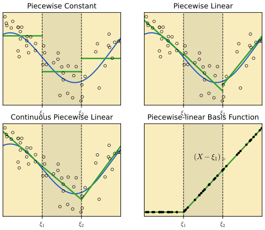
fig_5_1. Reproduces Hastie, Tibshirani and Friedman (2009), Figure 5.1. Download: PDF · SVGSmoother functions come from higher-order pieces with more continuity. Figure 5.2 fits piecewise cubics with increasing smoothness at the knots; the last one, continuous with continuous first and second derivatives, is a cubic spline. One more order of continuity would make it a single global cubic. The basis
\[ h_1(X)=1,\quad h_2(X)=X,\quad h_3(X)=X^2,\quad h_4(X)=X^3,\quad h_5(X)=(X-\xi_1)_+^3,\quad h_6(X)=(X-\xi_2)_+^3 \tag{5.3} \]spans the cubic splines with knots \(\xi_1,\xi_2\) (Exercise 5.1); the count \[(3\text{ regions})\times(4\text{ parameters})-(2\text{ knots})\times(3\text{ constraints})=6\] agrees.
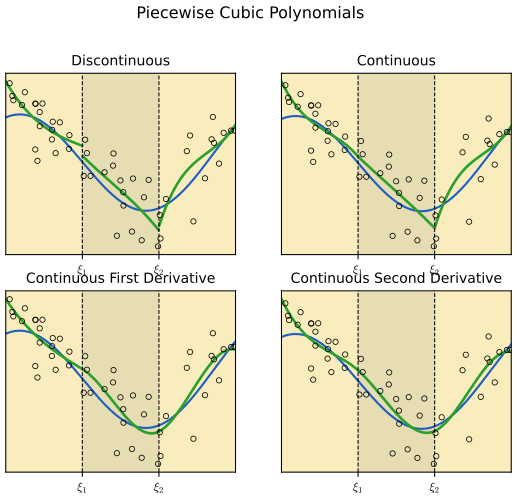
fig_5_2. Reproduces Hastie, Tibshirani and Friedman (2009), Figure 5.2. Download: PDF · SVGDefinition 5.2 (order-\(M\) spline, truncated power basis) p. 144
An order-\(M\) spline with knots \(\xi_1\lt\dots\lt\xi_K\) is a function that is a polynomial of degree at most \(M-1\) on each of the \(K+1\) intervals cut out by the knots and has continuous derivatives up to order \(M-2\) (for \(M=1\): piecewise constant, no continuity). Cubic splines have \(M=4\); the continuous piecewise linear functions of Result 5.1 are order-2 splines. The truncated power basis is
\[ h_j(X)=X^{j-1},\ j=1,\dots,M,\qquad h_{M+\ell}(X)=(X-\xi_\ell)_+^{M-1},\ \ell=1,\dots,K, \]with the convention \((X-\xi)_+^0=I(X\ge\xi)\). Fixed-knot splines fitted by least squares are called regression splines.
Result 5.2 (the truncated power basis is a basis; dimension \(M+K\); Exercise 5.1) pp. 143–144
The order-\(M\) splines with knots \(\xi_1,\dots,\xi_K\) form a vector space of dimension \(M+K\), and the \(M+K\) truncated power functions are a basis.
Proof
They are splines. \(X^{j-1}\) is a polynomial. \((X-\xi_\ell)_+^{M-1}\) is the polynomial 0 left of \(\xi_\ell\) and \((X-\xi_\ell)^{M-1}\) right of it; its derivatives of order \(r\le M-2\) are \(c_r(X-\xi_\ell)_+^{M-1-r}\), continuous because the exponent is \(\ge1\). So every combination is an order-\(M\) spline.
They span. Let \(f\) be an order-\(M\) spline, \(p_0,\dots,p_K\) its polynomial pieces from left to right. At \(\xi_\ell\) the difference \(q=p_\ell-p_{\ell-1}\) is a polynomial of degree \(\le M-1\) with \(q^{(r)}(\xi_\ell)=0\) for \(r=0,\dots,M-2\) (the continuity conditions). Its Taylor expansion at \(\xi_\ell\) therefore has only the top term: \(q(X)=\theta_\ell(X-\xi_\ell)^{M-1}\) with \(\theta_\ell=q^{(M-1)}/(M-1)!\). Then \(g(X)=p_0(X)+\sum_\ell\theta_\ell(X-\xi_\ell)_+^{M-1}\) equals \(p_0\) on the first interval, and on interval \(\ell\) it equals \(p_0+\sum_{k\le\ell}(p_k-p_{k-1})=p_\ell\). So \(f=g\) is in the span.
They are independent. If \(\sum_j\beta_jX^{j-1}+\sum_\ell\theta_\ell(X-\xi_\ell)_+^{M-1}\equiv0\), then on the first interval the polynomial \(\sum_j\beta_jX^{j-1}\) vanishes, so all \(\beta_j=0\); then on \((\xi_1,\xi_2)\) only \(\theta_1(X-\xi_1)^{M-1}\) remains, so \(\theta_1=0\), and so on. Hence the dimension is \(M+K\); the count "\(M(K+1)\) coefficients minus \((M-1)K\) constraints" gives the same number. ∎
Choosing the knots. One needs the order, the number of knots and their positions. A simple rule fixes the degrees of freedom and places the knots at quantiles of the \(x_i\): R's bs(x, df=7) returns cubic B-splines with \(7-3=4\) interior knots at the 20th, 40th, 60th and 80th percentiles. (A cubic spline with four knots is 8-dimensional; bs() drops the constant because the model usually contains an intercept.)
Filling the gap 5.3: why the truncated power basis is numerically poor p. 144
Explanation and a number
All the truncated power functions \((X-\xi_\ell)_+^3\) with knots to the left of a point grow like \(X^3\) there, so for large \(X\) the columns of \(\bH\) are nearly proportional; and the powers \(X^j\) of large numbers differ by orders of magnitude. Both make \(\bH^\T\bH\) nearly singular. B-splines (Appendix) span the same space, but each is non-zero on at most \(M\) adjacent intervals and bounded by 1, so the columns are nearly orthogonal. Confirmed numerically: for 200 points uniform on \([20,80]\) and eight knots at the deciles, the condition number of \(\bH\) is \(4.5\times10^{8}\) for the truncated power basis and \(5.3\) for the B-spline basis, while the two least-squares fits coincide (same column space).
See also (companion course): Filling the gap 3.2 on the SVD and numerical trouble in least squares.
5.2.1 Natural Cubic Splines
pp. 144–146 Polynomials fitted to data behave erratically near the boundaries, and cubic splines beyond the boundary knots are worse. The pointwise variance makes this precise.
Filling the gap 5.4: the pointwise variance of a least-squares fit p. 145, Figure 5.3
Derivation
Fix the inputs and let \(y_i=f(x_i)+\varepsilon_i\) with uncorrelated errors of variance \(\sigma^2\). With basis vector \(\bh(x)=(h_1(x),\dots,h_M(x))^\T\) and full-rank \(\bH\), \(\hat\bbeta=(\bH^\T\bH)^{-1}\bH^\T\y\) has \[\cov(\hat\bbeta)=(\bH^\T\bH)^{-1}\bH^\T(\sigma^2\bI)\bH(\bH^\T\bH)^{-1}=\sigma^2(\bH^\T\bH)^{-1}\], so
\[ \var\hat f(x_0)=\var\big(\bh(x_0)^\T\hat\bbeta\big)=\sigma^2\,\bh(x_0)^\T(\bH^\T\bH)^{-1}\bh(x_0). \]At the data, \[\sum_i\bh(x_i)^\T(\bH^\T\bH)^{-1}\bh(x_i)=\Tr\big(\bH(\bH^\T\bH)^{-1}\bH^\T\big)=M\]: the average pointwise variance at the inputs is \(\sigma^2M/N\) whatever the basis, so a model can only move variance around, not remove it. Splines move it to the boundary, where no data on the far side pin the cubic down. (In Figure 5.3, \(\sigma^2=1\); the sums at the data are 2, 4, 6 and 6, confirmed numerically.) ∎
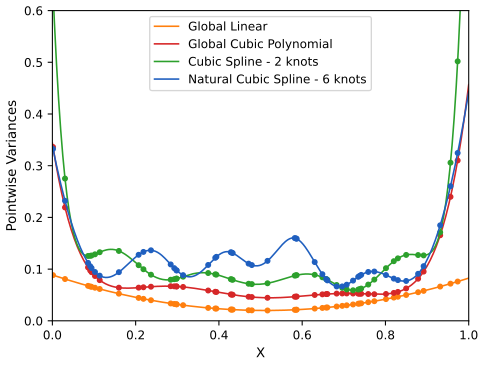
fig_5_3 (this is Exercise 5.3). Reproduces Hastie, Tibshirani and Friedman (2009), Figure 5.3. Download: PDF · SVGDefinition 5.3 (natural cubic spline) p. 145
A natural cubic spline with knots \(\xi_1\lt\dots\lt\xi_K\) is a cubic spline that is linear on \((-\infty,\xi_1]\) and on \([\xi_K,\infty)\). Equivalently, \(f''\) and \(f'''\) vanish beyond the boundary knots (the four "natural boundary conditions").
Result 5.3 (natural cubic splines have dimension \(K\); the basis (5.4)–(5.5)) pp. 145–146, Exercise 5.4
The natural cubic splines with \(K\ge2\) knots form a \(K\)-dimensional space, with basis
\[ N_1(X)=1,\qquad N_2(X)=X,\qquad N_{k+2}(X)=d_k(X)-d_{K-1}(X),\quad k=1,\dots,K-2, \tag{5.4} \] \[ d_k(X)=\frac{(X-\xi_k)_+^3-(X-\xi_K)_+^3}{\xi_K-\xi_k}. \tag{5.5} \]Proof
Write a cubic spline with the knots \(\xi_1,\dots,\xi_K\) in the truncated power basis, \[f(X)=\sum_{j=0}^3\beta_jX^j+\sum_{k=1}^K\theta_k(X-\xi_k)_+^3\] (5.70). For \(X\lt\xi_1\), \(f=\sum_j\beta_jX^j\), which is linear iff \(\beta_2=\beta_3=0\). For \(X\gt\xi_K\), expand \[(X-\xi_k)^3=X^3-3\xi_kX^2+3\xi_k^2X-\xi_k^3\]: the cubic coefficient is \(\beta_3+\sum_k\theta_k\) and the quadratic one \(\beta_2-3\sum_k\xi_k\theta_k\). With \(\beta_2=\beta_3=0\), linearity on the right is \(\sum_k\theta_k=0\) and \(\sum_k\xi_k\theta_k=0\). These are the constraints (5.71). They are four independent linear constraints on the \(K+4\) coefficients (the first two involve only \(\beta_2,\beta_3\); the last two only \(\bth\), and the vectors \((1,\dots,1)\) and \((\xi_1,\dots,\xi_K)\) are independent because the knots are distinct), so the space has dimension \(K+4-4=K\).
The basis. The constrained \(\bth\) form a \((K-2)\)-dimensional space. Each \(d_k\) (5.5) is a combination of two truncated cubics whose coefficients sum to zero, so \(d_k-d_{K-1}\) satisfies \(\sum\theta=0\); its weighted sum is \(\frac{\xi_k-\xi_K}{\xi_K-\xi_k}-\frac{\xi_{K-1}-\xi_K}{\xi_K-\xi_{K-1}}=-1+1=0\), so the \(\xi\)-weighted constraint holds too. Each \(N_{k+2}\) therefore is a natural cubic spline. They are independent: \(N_{k+2}\) is the only one with a non-zero coefficient on \((X-\xi_k)_+^3\) for \(k\le K-2\). Together with 1 and \(X\) they are \(K\) independent elements of a \(K\)-dimensional space, hence a basis. ∎
Linearity beyond the boundary knots frees four degrees of freedom (two in each tail), which can be spent on more interior knots; the price is some bias near the boundary, where the data carry little information anyway. Result 5.5 below gives a deeper reason for the boundary conditions: the curvature-penalised fit chooses them on its own.
5.2.2 Example: South African Heart Disease (Continued)
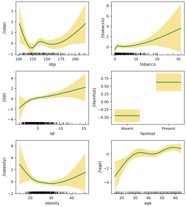
pp. 146–148 The linear logistic model of Section 4.4.2 is extended to
\[ \operatorname{logit}[\Pr(\text{chd}\given X)]=\theta_0+h_1(X_1)^\T\bth_1+h_2(X_2)^\T\bth_2+\dots+h_p(X_p)^\T\bth_p, \tag{5.6} \]where each \(h_j\) is a natural-spline basis with four functions (no constant): three interior knots at the quartiles of \(X_j\) and boundary knots at its extremes. The binary famhist has a single coefficient. Stacking the bases gives one \(N\times\df\) matrix \(\bH\), \(\df=1+\sum_j\df_j\), and the model is an ordinary linear logistic regression fitted by IRLS. Starting from the seven predictors of Section 4.4.2, terms are deleted backwards, a whole spline term at a time, as long as AIC \(=\) deviance \(+\,2\,\df\) decreases.
Table 5.1, reproduced: the final model after stepwise deletion p. 148
| Term deleted | Df | Deviance | AIC | LRT | P-value |
|---|---|---|---|---|---|
| none | 458.09 | 502.09 | |||
| sbp | 4 | 467.16 | 503.16 | 9.076 | 0.059 |
| tobacco | 4 | 470.48 | 506.48 | 12.387 | 0.015 |
| ldl | 4 | 472.39 | 508.39 | 14.307 | 0.006 |
| famhist | 1 | 479.44 | 521.44 | 21.356 | 0.000 |
| obesity | 4 | 466.24 | 502.24 | 8.147 | 0.086 |
| age | 4 | 481.86 | 517.86 | 23.768 | 0.000 |
Our own natural-spline basis, IRLS and stepwise search reproduce every entry of the book's table (only alcohol is deleted, at the first step: AIC 509.63 to 502.09); the deviance also agrees with R's glm with ns(df = 4) to \(10^{-6}\). The LRT column is the increase in deviance, referred to \(\chi^2_{\df}\).
Filling the gap 5.5: the standard-error bands of Figure 5.4 p. 146
Derivation
At the maximum likelihood estimate the IRLS iteration satisfies \(\hat\bth=(\bH^\T\bW\bH)^{-1}\bH^\T\bW\bz\) with working response \(\bz\) and weights \(w_i=\hat p_i(1-\hat p_i)\); the observed and expected information are both \(\bH^\T\bW\bH\), so the large-sample covariance is \(\hat\Sigma=(\bH^\T\bW\bH)^{-1}\). Each term \(\hat f_j(X_j)=h_j(X_j)^\T\hat\bth_j\) uses only the block \(\hat\Sigma_{jj}\), so \(v_j(X_j)=h_j(X_j)^\T\hat\Sigma_{jj}h_j(X_j)\) and the band is \(\hat f_j\pm2\sqrt{v_j}\). A term is only identified up to an additive constant (the intercept absorbs constants), so we plot the centred term \((h_j(x)-\bar h_j)^\T\hat\bth_j\), \(\bar h_j\) the average basis vector over the data, and its variance \((h_j(x)-\bar h_j)^\T\hat\Sigma_{jj}(h_j(x)-\bar h_j)\). ∎
sbp and low obesity is the retrospective-sampling effect discussed in the book (measurements taken after a heart attack, often after a change of lifestyle). Code: fig_5_4, sa_stepwise. Reproduces Hastie, Tibshirani and Friedman (2009), Figure 5.4. Download: PDF · SVGSee also (companion course): iteratively reweighted least squares.
5.2.3 Example: Phoneme Recognition
pp. 148–150 Here splines reduce flexibility. Each input is a log-periodogram \(x\in\R^{256}\), the values of a function \(X(f)\) of frequency on a grid; the task is to separate the phonemes "aa" (695 examples) and "ao" (1022). Logistic regression on the 256 values is a discretisation of a functional model:
\[ \log\frac{\Pr(\text{aa}\given X)}{\Pr(\text{ao}\given X)}=\int X(f)\beta(f)\,\d f, \tag{5.7} \] \[ \sum_{j=1}^{256}X(f_j)\beta(f_j)=\sum_{j=1}^{256}x_j\beta_j. \tag{5.8} \]The maximum likelihood coefficients are very rough (grey curve in Figure 5.5), and with 1000 training cases there are only about four observations per coefficient. The remedy is to force \(\beta(f)\) to be smooth: \(\beta(f)=\sum_{m=1}^Mh_m(f)\theta_m\), i.e. \(\bbeta=\bH\bth\) with \(\bH\) the \(256\times M\) matrix of natural cubic splines evaluated at the frequencies (\(M=12\), knots evenly spaced over \(1,\dots,256\)).
Result 5.4 (a restricted coefficient vector is a filtered input) p. 150
For any fixed \(p\times M\) matrix \(\bH\), fitting a linear (or logistic) model in \(x\) with coefficients constrained to \(\bbeta=\bH\bth\) is the same as fitting an unconstrained model in the filtered inputs \(x^*=\bH^\T x\in\R^M\); the fitted coefficient curve is \(\hat\beta(f)=\bh(f)^\T\hat\bth\).
Proof
The model depends on \(\bbeta\) only through \(x^\T\bbeta=x^\T\bH\bth=(\bH^\T x)^\T\bth\). So the likelihood of \((\beta_0,\bbeta=\bH\bth)\) on the data \((x_i,y_i)\) equals the likelihood of \((\beta_0,\bth)\) on \((\bH^\T x_i,y_i)\) for every \(\bth\), and the maximisers correspond. If \(\bH\) has full column rank, \(\bth\mapsto\bH\bth\) is one-to-one, so \(\hat\bth\) is unique whenever the filtered problem has a unique solution. ∎
Filling the gap 5.6: why positively correlated inputs give negatively correlated, rough coefficients p. 150
Derivation for a model case
Take a linear model with Gaussian errors and inputs whose covariance is the AR(1) matrix \(\Sigma_{jk}=\rho^{|j-k|}\), \(0\lt\rho\lt1\) (neighbouring frequencies strongly correlated). For large \(N\), \(\cov(\hat\bbeta)\approx\frac{\sigma^2}{N}\Sigma^{-1}\). The inverse of the AR(1) matrix is tridiagonal,
\[ \Sigma^{-1}=\frac1{1-\rho^2}\begin{pmatrix}1&-\rho&&\\-\rho&1+\rho^2&-\rho&\\&\ddots&\ddots&\ddots\\&&-\rho&1\end{pmatrix}, \](multiply it by \(\Sigma\) to check), so the correlation of two interior neighbouring coefficients is \(-\rho/(1+\rho^2)\lt0\). Estimation errors therefore alternate in sign from one frequency to the next: the jagged grey curve. A smoothness constraint removes exactly these high-frequency error components. ∎
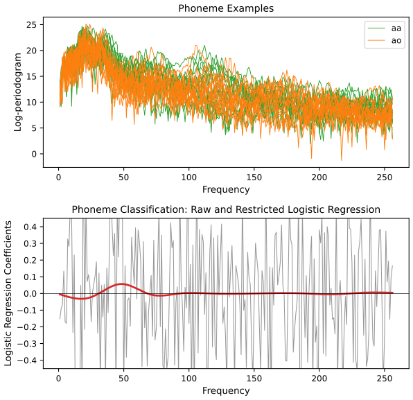
fig_5_5, phoneme_fits. Reproduces Hastie, Tibshirani and Friedman (2009), Figure 5.5. Download: PDF · SVGA sign convention in Figure 5.5
With the orientation of (5.7) (log odds of "aa" against "ao"), the fitted smooth coefficient curve is positive around frequency 45 and negative around 20: at frequency 45 the "aa" log-periodograms are on average 2.9 units higher than the "ao" ones, so a positive coefficient there is what (5.7) requires. The book's red curve has the opposite sign (positive near 20, negative near 45). It is the mirror image of ours, i.e. the coefficients of \(\log\{\Pr(\text{ao}\given X)/\Pr(\text{aa}\given X)\}\), which is what a fit treating the second factor level "ao" as the "success" produces. The shape and the conclusion (low frequencies discriminate) are unaffected.
5.3 Filtering and Feature Extraction
pp. 150–151 Result 5.4 is an instance of a general idea: replace raw high-dimensional features \(x\) by derived features \(x^*=g(x)\) and feed those to any learning method. The filter can be linear, \(x^*=\bH^\T x\) (splines as above, wavelets in Section 5.9, principal components), or nonlinear. Domain knowledge enters through the choice of \(g\): smoothness across frequency for spectra, localisation in time and scale (wavelets) for signals and images with edges. The derived features may then go into a linear or a nonlinear method (e.g. a neural network, Chapter 11).
Exercise 5.5 at the end of the chapter carries this out with quadratic discriminant analysis on the filtered phoneme features: filtering turns QDA from useless (test error 0.38 on the 256 raw inputs) into competitive (0.19).
5.4 Smoothing Splines
pp. 151–153 Smoothing splines avoid knot selection altogether: they use the maximal set of knots and control complexity by a penalty. Among all functions with two continuous derivatives, minimise the penalised residual sum of squares
\[ \RSS(f,\lambda)=\sum_{i=1}^N\{y_i-f(x_i)\}^2+\lambda\int\{f''(t)\}^2\,\d t, \tag{5.9} \]with smoothing parameter \(\lambda\ge0\). For \(\lambda=0\) any interpolating function is a minimiser; for \(\lambda=\infty\) no curvature is tolerated and the solution is the least-squares line. The problem is posed over an infinite-dimensional (Sobolev) space, yet its solution is finite-dimensional.
Result 5.5 (the smoothing-spline theorem; Exercise 5.7) p. 151
Let \(t_1\lt\dots\lt t_n\) be the distinct values among \(x_1,\dots,x_N\), with \(n\ge2\), and \(\lambda\gt0\). Over all \(f\) on \([a,b]\supset[t_1,t_n]\) with \(f'\) absolutely continuous and \(f''\in L^2\), (5.9) has a unique minimiser, and it is a natural cubic spline with knots at \(t_1,\dots,t_n\).
Proof
Step 1 (an identity). Let \(g\) be a natural cubic spline with knots \(t_1,\dots,t_n\) and \(h\) any function in the class with \(h(t_j)=0\) for all \(j\). Integrate by parts on \([t_1,t_n]\) (outside it \(g''=0\)):
\[ \int_a^bg''h''=\big[g''h'\big]_{t_1}^{t_n}-\int_{t_1}^{t_n}g'''h'=-\sum_{j=1}^{n-1}g'''(t_j^+)\int_{t_j}^{t_{j+1}}h'=-\sum_{j=1}^{n-1}g'''(t_j^+)\{h(t_{j+1})-h(t_j)\}=0. \]The boundary term vanishes because \(g''(t_1)=g''(t_n)=0\) (natural spline), \(g'''\) is constant on each \((t_j,t_{j+1})\) because \(g\) is cubic there, and the last sum vanishes because \(h\) is zero at every knot. This is (5.72).
Step 2 (minimum roughness interpolation). Given values \(z_1,\dots,z_n\), there is exactly one natural cubic spline \(g\) with \(g(t_j)=z_j\) (the natural splines with \(n\) knots form an \(n\)-dimensional space, Result 5.3, and the evaluation map is injective: by Step 1 with \(h=g\), a natural spline vanishing at all knots has \(\int g''^2=0\), so \(g\) is linear and, vanishing at two points, zero). If \(\tilde g\) is any other interpolant in the class and \(h=\tilde g-g\), Step 1 gives
\[ \int\tilde g''^2=\int g''^2+2\int g''h''+\int h''^2=\int g''^2+\int h''^2\ \ge\ \int g''^2, \]with equality iff \(h''\equiv0\), i.e. \(h\) linear; since \(h\) vanishes at \(n\ge2\) points, \(h\equiv0\).
Step 3 (the minimiser). For any \(f\) in the class let \(g\) be the natural spline interpolating \(f(t_1),\dots,f(t_n)\). The residual sums of squares of \(f\) and \(g\) are equal (they depend only on the values at the data), and by Step 2 \(\int g''^2\le\int f''^2\), strictly unless \(f=g\). So a minimiser, if it exists, is a natural spline, and the problem reduces to minimising over \(\bg=(g(t_1),\dots,g(t_n))\). By Result 5.6 below this is \((\y-\bP\bg)^\T(\y-\bP\bg)+\lambda\bg^\T\bK\bg\) (\(\bP\) the \(N\times n\) incidence matrix of ties), a quadratic with Hessian \(2(\bP^\T\bP+\lambda\bK)\). This is positive definite: \(\bP^\T\bP=\diag(\text{counts})\) is, and \(\bK\) is positive semidefinite. Hence there is exactly one minimiser. ∎
Since the solution is a natural spline with \(N\) knots (no ties), write it in an \(N\)-dimensional natural-spline basis,
\[ f(x)=\sum_{j=1}^NN_j(x)\theta_j, \tag{5.10} \] \[ \RSS(\bth,\lambda)=(\y-\bN\bth)^\T(\y-\bN\bth)+\lambda\bth^\T\bOm_N\bth, \tag{5.11} \]with \(\{\bN\}_{ij}=N_j(x_i)\) and \(\{\bOm_N\}_{jk}=\int N_j''(t)N_k''(t)\,\d t\). Setting the gradient \(-2\bN^\T(\y-\bN\bth)+2\lambda\bOm_N\bth\) to zero gives the generalised ridge regression
\[ \hat\bth=(\bN^\T\bN+\lambda\bOm_N)^{-1}\bN^\T\y, \tag{5.12} \] \[ \hat f(x)=\sum_{j=1}^NN_j(x)\hat\theta_j. \tag{5.13} \]The matrix is invertible because \(\bN\) is square and invertible (Step 2 above). The penalty shrinks the coefficients toward the unpenalised linear part, which is why \(N\) knots do not mean \(N\) degrees of freedom.
See also (companion courses): ridge regression and its shrinkage factors, Section 3.1.4 and Section 4.1.6.
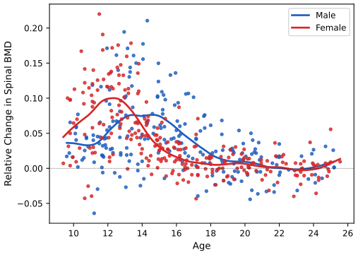
fig_5_6. Reproduces Hastie, Tibshirani and Friedman (2009), Figure 5.6. Download: PDF · SVGFilling the gap 5.7: \(\lambda\) has units; df does not pp. 152–154
Derivation
Rescale the input, \(u=cx\), and put \(\tilde f(u)=f(u/c)\). Then \(\tilde f''(u)=f''(x)/c^2\) and \(\d u=c\,\d x\), so \(\int\tilde f''(u)^2\d u=c^{-3}\int f''(x)^2\d x\). The fitted values are unchanged if \(\tilde\lambda c^{-3}=\lambda\), i.e. \(\tilde\lambda=c^3\lambda\). For the male bone data the ages span 15.6 years, so rescaling them to \([0,1]\) is \(c=1/15.6\), and \[\tilde\lambda=0.844/15.6^3\approx0.844/3800\approx0.00022\]. The effective degrees of freedom are invariant under this change, which is one reason the book (and R's smooth.spline) let the user specify df rather than \(\lambda\). ∎
5.4.1 Degrees of Freedom and Smoother Matrices
pp. 153–156 For fixed \(\lambda\) the fitted values are linear in \(\y\):
\[ \hat\bff=\bN(\bN^\T\bN+\lambda\bOm_N)^{-1}\bN^\T\y=\bS_\lambda\y. \tag{5.14} \]\(\bS_\lambda\) is the smoother matrix; it depends on the \(x_i\) and \(\lambda\), not on \(\y\). A regression spline with an \(N\times M\) basis matrix \(\bB_\xi\) of rank \(M\) has the projection (hat) matrix
\[ \hat\bff=\bB_\xi(\bB_\xi^\T\bB_\xi)^{-1}\bB_\xi^\T\y=\bH_\xi\y. \tag{5.15} \]Result 5.6 (the Reinsch form; Exercise 5.9) p. 154, (5.17)–(5.18)
With distinct sorted \(x_1\lt\dots\lt x_N\), \(h_j=x_{j+1}-x_j\), let \(\bQ\) be the \(N\times(N-2)\) matrix with non-zero entries \(q_{j-1,j}=1/h_{j-1}\), \(q_{jj}=-1/h_{j-1}-1/h_j\), \(q_{j+1,j}=1/h_j\), and \(\bR\) the symmetric tridiagonal \((N-2)\times(N-2)\) matrix with \(r_{jj}=(h_{j-1}+h_j)/3\), \(r_{j,j+1}=h_j/6\) (\(j=2,\dots,N-1\)). Then for the natural cubic spline \(g\) with values \(\bg\) at the knots,
\[ \int g''(t)^2\,\d t=\bg^\T\bK\bg,\qquad \bK=\bQ\bR^{-1}\bQ^\T=\bN^{-\T}\bOm_N\bN^{-1}, \]and the smoother matrix is
\[ \bS_\lambda=(\bI+\lambda\bK)^{-1}, \tag{5.17} \]where \(\bK\) does not depend on \(\lambda\); \(\hat\bff\) solves
\[ \min_\bff\,(\y-\bff)^\T(\y-\bff)+\lambda\bff^\T\bK\bff. \tag{5.18} \]Proof
Penalty in terms of values. Let \(\gamma_j=g''(x_j)\); \(\gamma_1=\gamma_N=0\). On \([x_j,x_{j+1}]\), \(g''\) is linear from \(\gamma_j\) to \(\gamma_{j+1}\), so integrating twice and matching \(g(x_j),g(x_{j+1})\),
\[ g(x)=\frac{(x-x_j)g_{j+1}+(x_{j+1}-x)g_j}{h_j}-\frac{(x-x_j)(x_{j+1}-x)}6\Big\{\Big(1+\frac{x-x_j}{h_j}\Big)\gamma_{j+1}+\Big(1+\frac{x_{j+1}-x}{h_j}\Big)\gamma_j\Big\}. \]Differentiating, \(g'(x_j^+)=\frac{g_{j+1}-g_j}{h_j}-\frac{h_j}6(2\gamma_j+\gamma_{j+1})\) and \(g'(x_{j+1}^-)=\frac{g_{j+1}-g_j}{h_j}+\frac{h_j}6(\gamma_j+2\gamma_{j+1})\). Continuity of \(g'\) at each interior knot \(x_j\) reads
\[ \frac{g_{j+1}-g_j}{h_j}-\frac{g_j-g_{j-1}}{h_{j-1}}=\frac{h_{j-1}}6\gamma_{j-1}+\frac{h_{j-1}+h_j}3\gamma_j+\frac{h_j}6\gamma_{j+1},\qquad j=2,\dots,N-1, \]which is \(\bQ^\T\bg=\bR\bgam\) for the interior vector \(\bgam=(\gamma_2,\dots,\gamma_{N-1})\). \(\bR\) is strictly diagonally dominant with positive diagonal, hence positive definite, so \(\bgam=\bR^{-1}\bQ^\T\bg\). (Continuity of \(g\) and \(g''\) is built into the formula, so these \(N-2\) equations are exactly the spline conditions.) Next, the integral of the square of a linear function from \(a\) to \(b\) over length \(h\) is \(h(a^2+ab+b^2)/3\), so
\[ \int g''^2=\sum_{j=1}^{N-1}\frac{h_j}3(\gamma_j^2+\gamma_j\gamma_{j+1}+\gamma_{j+1}^2)=\bgam^\T\bR\bgam=\bg^\T\bQ\bR^{-1}\bQ^\T\bg . \]Reinsch form. By Result 5.5, (5.9) is minimised over the values \(\bff=\bg\): \((\y-\bff)^\T(\y-\bff)+\lambda\bff^\T\bK\bff\), which is (5.18). Its gradient \(-2(\y-\bff)+2\lambda\bK\bff\) vanishes at \(\hat\bff=(\bI+\lambda\bK)^{-1}\y\), and \(\bI+\lambda\bK\) is positive definite. In the basis of (5.10), \(\bff=\bN\bth\) with \(\bN\) invertible, \(\bth^\T\bOm_N\bth=\int f''^2=\bff^\T\bK\bff\) for all \(\bth\), so \(\bOm_N=\bN^\T\bK\bN\); substituting into (5.14), \[\bS_\lambda=\bN(\bN^\T\bN+\lambda\bN^\T\bK\bN)^{-1}\bN^\T=(\bI+\lambda\bK)^{-1}\]. Both forms of \(\bK\) agree to \(10^{-6}\) relative error in our code. ∎
The Reinsch form is also how smoothing splines are computed: \((\bI+\lambda\bK)\hat\bff=\y\) is equivalent to the pentadiagonal system \((\bR+\lambda\bQ^\T\bQ)\bgam=\bQ^\T\y\), \(\hat\bff=\y-\lambda\bQ\bgam\), solvable in \(O(N)\) operations (Green and Silverman 1994). With ties, the distinct values carry weights \(w_j\) (the counts) and the responses are averaged (Exercise 5.12), giving \(\hat\bff=(\bW+\lambda\bK)^{-1}\bW\bar\y\).
Both \(\bH_\xi\) and \(\bS_\lambda\) are symmetric positive semidefinite. But \(\bH_\xi\bH_\xi=\bH_\xi\) (idempotent, rank \(M\)), while \(\bS_\lambda\bS_\lambda\preceq\bS_\lambda\) (rank \(N\)). By analogy with \(M=\Tr\bH_\xi\) the effective degrees of freedom of a smoothing spline are
\[ \df_\lambda=\Tr(\bS_\lambda). \tag{5.16} \]The eigen-decomposition of \(\bS_\lambda\) is
\[ \bS_\lambda=\sum_{k=1}^N\rho_k(\lambda)\bu_k\bu_k^\T \tag{5.19} \] \[ \rho_k(\lambda)=\frac1{1+\lambda d_k}, \tag{5.20} \]with \(d_k\) the eigenvalues of \(\bK\) and \(\bu_k\) its orthonormal eigenvectors.
Result 5.7 (spectral properties of the smoother; Exercise 5.11) pp. 154–156
(a) \(\bK\) is positive semidefinite with null space \(\{a\mathbf1+b\bx\}\) (the linear functions), so \(d_1=d_2=0\lt d_3\le\dots\le d_N\). (b) The eigenvectors \(\bu_k\) do not depend on \(\lambda\); \(\rho_1=\rho_2=1\) and \(0\lt\rho_k\lt1\) for \(k\ge3\). (c) \(\bS_\lambda-\bS_\lambda^2\succeq0\) and \(\df_\lambda=\sum_k\rho_k(\lambda)\in(2,N)\). (d) As \(\lambda\to0\), \(\bS_\lambda\to\bI\) and \(\df_\lambda\to N\); as \(\lambda\to\infty\), \(\bS_\lambda\to\bH\), the hat matrix of the least-squares line, and \(\df_\lambda\to2\). (e) In the Demmler–Reinsch basis \(\bU=(\bu_1,\dots,\bu_N)\), the fit solves
\[ \min_\bth\ \|\y-\bU\bth\|^2+\lambda\bth^\T\bD\bth,\qquad \bD=\diag(d_k). \tag{5.21} \]Proof
(a) \(\bg^\T\bK\bg=\int g''^2\ge0\), with equality iff \(g''\equiv0\), i.e. \(g\) is linear, i.e. \(\bg\) lies in \(\operatorname{span}\{\mathbf1,\bx\}\) (directly: \(\bQ^\T\bg\) is the vector of second divided differences, zero exactly for linear \(\bg\), and \(\bR^{-1}\) is positive definite). For distinct \(x_i\) (\(N\ge3\)) this null space has dimension 2.
(b) \((\bI+\lambda\bK)\bu_k=(1+\lambda d_k)\bu_k\), so \(\bS_\lambda\bu_k=\bu_k/(1+\lambda d_k)\): same eigenvectors for every \(\lambda\), eigenvalues (5.20), equal to 1 iff \(d_k=0\).
(c) \(\bS_\lambda-\bS_\lambda^2\) has eigenvalues \(\rho_k(1-\rho_k)\ge0\). The trace is the sum of eigenvalues: two equal to 1 and \(N-2\) in \((0,1)\).
(d) Each \(\rho_k\to1\) as \(\lambda\to0\), and \(\rho_k\to0\) for \(k\ge3\) as \(\lambda\to\infty\), leaving \(\bu_1\bu_1^\T+\bu_2\bu_2^\T\), the orthogonal projection onto \(\operatorname{span}\{\mathbf1,\bx\}\), which is \(\bH\).
(e) \(\bU\) is orthogonal, so with \(\bff=\bU\bth\), \(\|\y-\bff\|^2=\|\y-\bU\bth\|^2\) and \(\bff^\T\bK\bff=\bth^\T\bU^\T\bK\bU\bth=\bth^\T\bD\bth\); (5.18) becomes (5.21). Its solution is \(\hat\theta_k=\rho_k\langle\bu_k,\y\rangle\): the smoothing spline decomposes \(\y\) in the basis \(\bu_k\) and shrinks each component by \(\rho_k\), whereas a projection smoother keeps \(M\) components and kills the rest. ∎
Two further facts from Figure 5.7: ordered by decreasing \(\rho_k\), the \(\bu_k\) oscillate more and more (like orthogonal polynomials of increasing degree; on a periodic domain they would be sines and cosines), so the more complex a component, the more it is shrunk; and \(\lambda\) controls how fast \(\rho_k\) decays to zero.
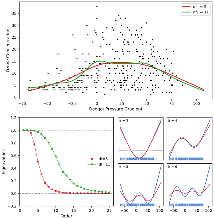
fig_5_7, class SmoothingSpline. Reproduces Hastie, Tibshirani and Friedman (2009), Figure 5.7. Download: PDF · SVGEquivalent kernels. Row \(i\) of \(\bS_\lambda\) gives the weights with which the \(y_j\) enter \(\hat f(x_i)\). Figure 5.8 shows that the smoother matrix is nearly banded: a smoothing spline is a local averaging method, like the kernel smoothers of Chapter 6, with a kernel that adapts its shape near the boundary.
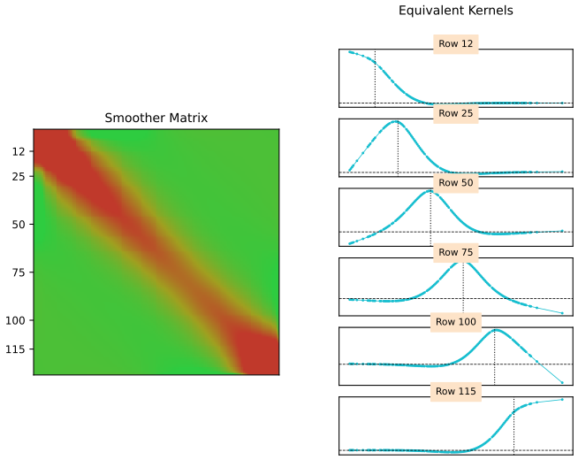
fig_5_8. Reproduces Hastie, Tibshirani and Friedman (2009), Figure 5.8. Download: PDF · SVGSee also (companion course): the equivalent kernel of Bayesian linear regression and the effective number of well-determined parameters \(\gamma=\sum\lambda_i/(\alpha+\lambda_i)\), the same sum of shrinkage factors as \(\df_\lambda\).
5.5 Automatic Selection of the Smoothing Parameters
pp. 156–158 For regression splines the smoothing parameters are the degree and the number and placement of knots, a combinatorial problem (MARS in Chapter 9 attacks it greedily). For smoothing splines only \(\lambda\) remains.
5.5.1 Fixing the Degrees of Freedom
Filling the gap 5.9: df is a strictly decreasing function of \(\lambda\), so it can be inverted p. 158
Derivation
\(\df_\lambda=2+\sum_{k\ge3}(1+\lambda d_k)^{-1}\) with \(d_k\gt0\), so \(\frac{\d}{\d\lambda}\df_\lambda=-\sum_{k\ge3}d_k(1+\lambda d_k)^{-2}\lt0\); it is continuous, tends to \(N\) as \(\lambda\to0\) and to 2 as \(\lambda\to\infty\). Hence for every target \(\df\in(2,N)\) there is exactly one \(\lambda\), found by a one-dimensional root finder (we use Brent's method on \(\log\lambda\), with \(\df\) evaluated in \(O(N)\) from the eigenvalues). This is what smooth.spline(x, y, df = 6) does in R; our fits agree with it to \(2\times10^{-4}\) (the tolerance of R's search). ∎
Specifying df instead of \(\lambda\) makes smoothers of different kinds comparable, and it is how several smoothers are combined in the generalised additive models of Chapter 9.
5.5.2 The Bias–Variance Tradeoff
pp. 158–161 Figure 5.9 uses the model
\[ Y=f(X)+\varepsilon,\qquad f(X)=\frac{\sin(12(X+0.2))}{X+0.2}, \tag{5.22} \]with \(X\sim U[0,1]\), \(\varepsilon\sim N(0,1)\) and \(N=100\). Since \(\hat\bff=\bS_\lambda\y\) and \(\cov(\y)=\sigma^2\bI\) (here \(\sigma^2=1\)),
\[ \cov(\hat\bff)=\bS_\lambda\cov(\y)\bS_\lambda^\T=\bS_\lambda\bS_\lambda^\T, \tag{5.23} \] \[ \Bias(\hat\bff)=\bff-\E(\hat\bff)=\bff-\bS_\lambda\bff. \tag{5.24} \]Result 5.8 (pointwise bias and variance anywhere; EPE; Exercise 5.10) pp. 158–160
For fixed inputs and any \(x_0\), \(\hat f_\lambda(x_0)=\bl(x_0)^\T\y\) for a weight vector \(\bl(x_0)\) (the equivalent kernel at \(x_0\)), and
\[ \var\hat f_\lambda(x_0)=\sigma^2\|\bl(x_0)\|^2,\qquad \Bias\hat f_\lambda(x_0)=f(x_0)-\bl(x_0)^\T\bff . \]With Gaussian errors, \(\hat f_\lambda(x_0)\sim N\big(\bl(x_0)^\T\bff,\ \sigma^2\|\bl(x_0)\|^2\big)\) exactly. For a new pair \((X,Y)\) independent of the training data,
\[ \EPE(\hat f_\lambda)=\E(Y-\hat f_\lambda(X))^2=\var(Y)+\E\big[\Bias^2(\hat f_\lambda(X))+\var(\hat f_\lambda(X))\big]=\sigma^2+\MSE(\hat f_\lambda). \tag{5.25} \]Proof
The fitted spline is determined linearly by \(\hat\bff=\bS_\lambda\y\): its value anywhere is a linear function of the values at the knots (the formula in the proof of Result 5.6, with \(\bgam=\bR^{-1}\bQ^\T\hat\bff\)). So \(\hat f_\lambda(x_0)=\bl(x_0)^\T\y\), and \(\var(\bl^\T\y)=\bl^\T(\sigma^2\bI)\bl\), \(\E(\bl^\T\y)=\bl^\T\bff\). A linear function of a Gaussian vector is Gaussian. For (5.25) condition on \(X=x_0\): \[Y-\hat f(x_0)=\{Y-f(x_0)\}+\{f(x_0)-\E\hat f(x_0)\}+\{\E\hat f(x_0)-\hat f(x_0)\}\]; the first term is independent of the other two and has mean zero, the third has mean zero, so the cross terms vanish in expectation and \(\E[(Y-\hat f(x_0))^2]=\sigma^2+\Bias^2+\var\). Averaging over \(X\) gives (5.25). ∎
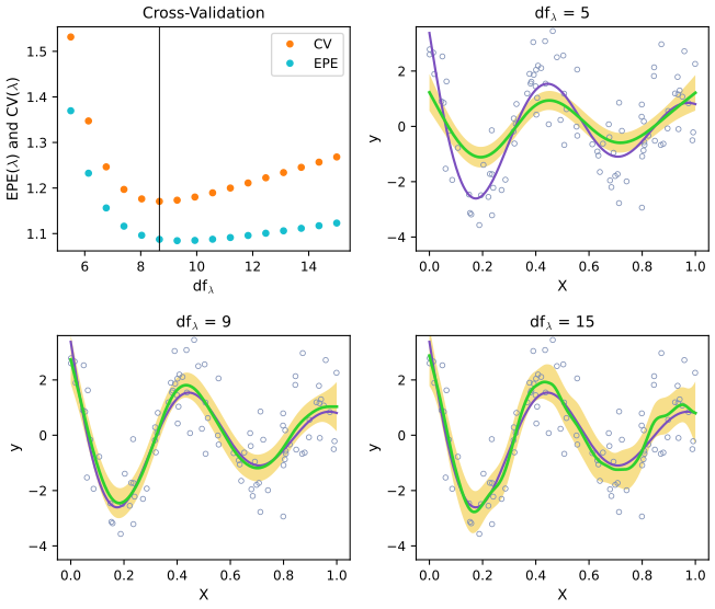
fig_5_9, epe_curve. Reproduces Hastie, Tibshirani and Friedman (2009), Figure 5.9. Download: PDF · SVGThe EPE curve of Figure 5.9 lies below \(\sigma^2\)
By (5.25), \(\EPE(\hat f_\lambda)=\sigma^2+\MSE\ge\sigma^2=1\) under the stated model \(\varepsilon\sim N(0,1)\). The book's EPE points, however, range from about 0.87 to 1.15, with the minimum near 0.87. So the plotted curve cannot be the EPE (5.25) of the model as stated (it may be a single test-sample estimate, or computed with a different noise level). Our exact EPE values are all above 1 (1.539, 1.085 and 1.123 at 5, 9 and 15 df), and a simulation of 400 replications confirms the value at 9 df (1.090). The qualitative message, a minimum near 9 df and a CV curve of similar shape, is unchanged.
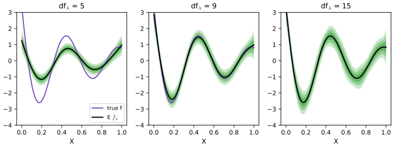
fig_5_S1. Download: PDF · SVGCross-validation. EPE is unknown in practice; Chapter 7 discusses K-fold CV, GCV and \(C_p\). For a smoothing spline the leave-one-out version is cheap:
\[ \CV(\hat f_\lambda)=\frac1N\sum_{i=1}^N\big(y_i-\hat f_\lambda^{(-i)}(x_i)\big)^2 \tag{5.26} \] \[ \phantom{\CV(\hat f_\lambda)}=\frac1N\sum_{i=1}^N\left(\frac{y_i-\hat f_\lambda(x_i)}{1-S_\lambda(i,i)}\right)^2. \tag{5.27} \]Result 5.9 (leave-one-out from a single fit; Exercise 5.13) p. 161
(a) If the fit \(\hat f_\lambda\) to the \(N\) pairs is augmented by the pair \((x_0,\hat f_\lambda(x_0))\) and the spline is refitted with the same \(\lambda\), the fit does not change. (b) Consequently \(\hat f^{(-i)}_\lambda(x_i)\) is the full-data fit with \(y_i\) replaced by \(\hat f^{(-i)}_\lambda(x_i)\), and (5.26) equals (5.27).
Proof
(a) Write \(C(f)=\sum_i(y_i-f(x_i))^2+\lambda J(f)\) and \(C_0(f)=C(f)+(\hat f(x_0)-f(x_0))^2\). For every \(f\), \(C_0(f)\ge C(f)\ge C(\hat f)=C_0(\hat f)\), so \(\hat f\) minimises \(C_0\); the minimiser is unique (Result 5.5), so it is the refit.
(b) Apply (a) to the \(N-1\) pairs without \(i\), with \(x_0=x_i\): \(\hat f^{(-i)}\) also minimises the full criterion with \(y_i\) replaced by \(y_i^*=\hat f^{(-i)}(x_i)\). The full fit is linear with smoother \(\bS_\lambda\), so
\[ \hat f^{(-i)}(x_i)=\sum_{j\ne i}S_{ij}y_j+S_{ii}\hat f^{(-i)}(x_i)=\hat f(x_i)-S_{ii}y_i+S_{ii}\hat f^{(-i)}(x_i). \]Solving, \(\hat f^{(-i)}(x_i)=\{\hat f(x_i)-S_{ii}y_i\}/(1-S_{ii})\), hence \[y_i-\hat f^{(-i)}(x_i)=\{y_i-\hat f(x_i)\}/(1-S_{ii})\]. Here \(S_{ii}=\sum_k\rho_ku_{ik}^2\le\sum_ku_{ik}^2=1\), with equality only if \(\mathbf e_i\in\operatorname{span}\{\mathbf1,\bx\}\), impossible for \(N\ge3\) distinct inputs; so the division is legitimate. Nothing in the argument is specific to splines: it holds for every penalised least-squares fit with a unique solution, including ridge regression and the weighted spline with ties (both confirmed numerically against \(N\) explicit refits). ∎
The CV curve of Figure 5.9 lies above EPE for this sample; over realisations CV is approximately unbiased for EPE (computed on a training set of size \(N-1\)). Generalised cross-validation replaces each \(S_{ii}\) by their average \(\df_\lambda/N\).
See also (companion courses): the bias–variance decomposition, Bishop (2006) Section 3.2 and Bishop and Bishop (2024) Section 4.3.
5.6 Nonparametric Logistic Regression
pp. 161–162 With a binary response and one quantitative input, model the log odds by a smooth function,
\[ \log\frac{\Pr(Y=1\given X=x)}{\Pr(Y=0\given X=x)}=f(x), \tag{5.28} \] \[ \Pr(Y=1\given X=x)=\frac{e^{f(x)}}{1+e^{f(x)}}, \tag{5.29} \]and maximise the penalised log-likelihood (\(p(x)=\Pr(Y=1\given x)\))
\[ \ell(f;\lambda)=\sum_{i=1}^N\big[y_i\log p(x_i)+(1-y_i)\log(1-p(x_i))\big]-\tfrac12\lambda\int\{f''(t)\}^2\d t=\sum_{i=1}^N\big[y_if(x_i)-\log(1+e^{f(x_i)})\big]-\tfrac12\lambda\int\{f''(t)\}^2\d t. \tag{5.30} \]Result 5.10 (penalised logistic regression is iterated weighted smoothing) pp. 161–162, (5.31)–(5.34); Exercise 5.12
(a) The maximiser of (5.30) is a natural cubic spline with knots at the distinct \(x_i\); writing \(f=\sum_jN_j\theta_j\),
\[ \frac{\partial\ell(\bth)}{\partial\bth}=\bN^\T(\y-\bp)-\lambda\bOm\bth, \tag{5.31} \] \[ \frac{\partial^2\ell(\bth)}{\partial\bth\partial\bth^\T}=-\bN^\T\bW\bN-\lambda\bOm, \tag{5.32} \]with \(\bW=\diag\{p(x_i)(1-p(x_i))\}\). (b) \(\ell\) is strictly concave, and the Newton–Raphson step is
\[ \bth^{\rm new}=(\bN^\T\bW\bN+\lambda\bOm)^{-1}\bN^\T\bW\big(\bN\bth^{\rm old}+\bW^{-1}(\y-\bp)\big)=(\bN^\T\bW\bN+\lambda\bOm)^{-1}\bN^\T\bW\bz, \tag{5.33} \] \[ \bff^{\rm new}=\bN(\bN^\T\bW\bN+\lambda\bOm)^{-1}\bN^\T\bW\big(\bff^{\rm old}+\bW^{-1}(\y-\bp)\big)=\bS_{\lambda,w}\bz, \tag{5.34} \]a weighted smoothing spline of the working response \(\bz\) with weights \(w_i\). (c) The weighted smoothing spline, the minimiser of \(\sum_iw_i\{y_i-f(x_i)\}^2+\lambda\int f''^2\) (5.73), has fitted values \((\bW+\lambda\bK)^{-1}\bW\y\).
Proof
(a) The log-likelihood depends on \(f\) only through the values \(f(x_i)\); replacing \(f\) by the natural spline interpolating those values keeps it and does not increase the penalty (Step 2 of Result 5.5), strictly unless \(f\) is that spline. The derivative of \(y\eta-\log(1+e^\eta)\) in \(\eta\) is \(y-p\) and the second derivative \(-p(1-p)\); with \(\eta_i=\sum_jN_{ij}\theta_j\) the chain rule gives \(\bN^\T(\y-\bp)\) and \(-\bN^\T\bW\bN\), and the penalty \(\tfrac12\lambda\bth^\T\bOm\bth\) contributes \(-\lambda\bOm\bth\) and \(-\lambda\bOm\).
(b) \(\bN\) is invertible and \(\bW\) has positive diagonal, so \(\bN^\T\bW\bN\) is positive definite and (5.32) is negative definite: \(\ell\) is strictly concave, the maximiser is unique. Newton: \[\bth^{\rm new}=\bth^{\rm old}+(\bN^\T\bW\bN+\lambda\bOm)^{-1}\{\bN^\T(\y-\bp)-\lambda\bOm\bth^{\rm old}\}\]. Writing \[\bth^{\rm old}=(\bN^\T\bW\bN+\lambda\bOm)^{-1}(\bN^\T\bW\bN+\lambda\bOm)\bth^{\rm old}\] and collecting terms gives (5.33); multiplying by \(\bN\) gives (5.34).
(c) As in Result 5.5 the minimiser of (5.73) is a natural spline (if some \(w_i=0\), drop those points; at least two distinct inputs with positive weight are needed). In terms of its values it minimises \((\y-\bff)^\T\bW(\y-\bff)+\lambda\bff^\T\bK\bff\), whose stationarity condition is \((\bW+\lambda\bK)\bff=\bW\y\); and \[\bN(\bN^\T\bW\bN+\lambda\bOm)^{-1}\bN^\T\bW=(\bW+\lambda\bK)^{-1}\bW\] by \(\bOm=\bN^\T\bK\bN\). Ties: observations sharing an input \(t_j\) combine into one weight \(\sum w_i\) and the weighted mean response, since \[\sum_{i:x_i=t_j}w_i(y_i-f)^2=(\sum w_i)(\bar y_j-f)^2+\text{const}\]. ∎
The form (5.34) suggests replacing \(\bS_{\lambda,w}\) by any weighted nonparametric regression operator: this is the local-scoring algorithm behind generalised additive models (Chapter 9).
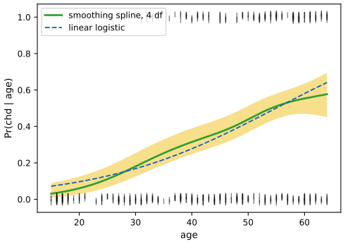
fig_5_S2, nonparametric_logistic. Download: PDF · SVGSee also (companion course): IRLS for logistic regression and the logistic regression demo.
5.7 Multidimensional Splines
pp. 162–167 With \(X\in\R^2\) and bases \(h_{1j}(X_1)\), \(j=1,\dots,M_1\), and \(h_{2k}(X_2)\), \(k=1,\dots,M_2\), the tensor product basis
\[ g_{jk}(X)=h_{1j}(X_1)h_{2k}(X_2),\qquad j=1,\dots,M_1,\ k=1,\dots,M_2 \tag{5.35} \]represents two-dimensional functions as
\[ g(X)=\sum_{j=1}^{M_1}\sum_{k=1}^{M_2}\theta_{jk}g_{jk}(X). \tag{5.36} \]The coefficients are fitted by least squares as before. In \(d\) dimensions with \(M\) functions per coordinate the basis has \(M^d\) elements: the curse of dimensionality again (MARS, Chapter 9, adds tensor products greedily instead).
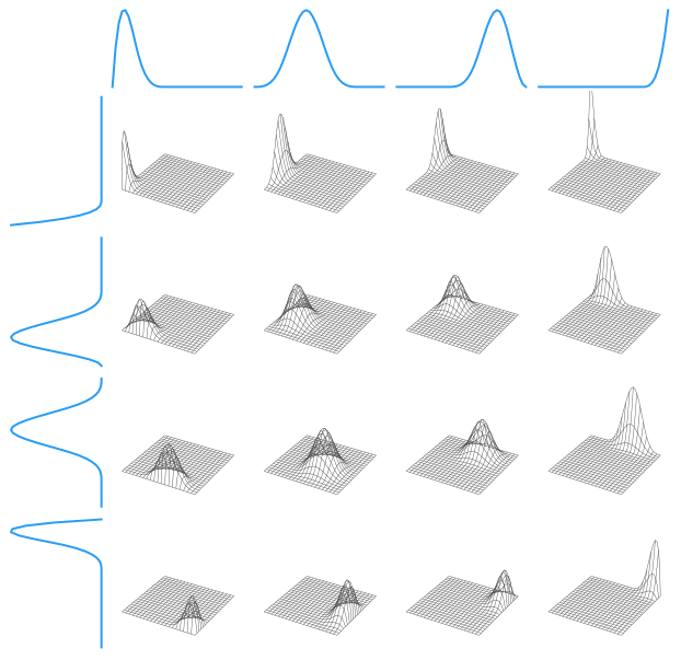
fig_5_10. Reproduces Hastie, Tibshirani and Friedman (2009), Figure 5.10. Download: PDF · SVG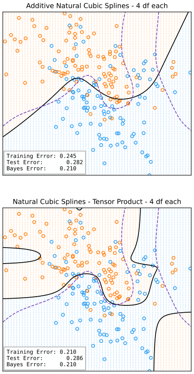
fig_5_11, mixture_spline_models. Reproduces Hastie, Tibshirani and Friedman (2009), Figure 5.11. Download: PDF · SVGThin-plate splines. Smoothing splines generalise too: for \(x_i\in\R^d\) solve
\[ \min_f\sum_{i=1}^N\{y_i-f(x_i)\}^2+\lambda J[f], \tag{5.37} \]with, in two dimensions, the rotation-invariant roughness penalty
\[ J[f]=\iint_{\R^2}\Big[\Big(\frac{\partial^2f}{\partial x_1^2}\Big)^2+2\Big(\frac{\partial^2f}{\partial x_1\partial x_2}\Big)^2+\Big(\frac{\partial^2f}{\partial x_2^2}\Big)^2\Big]\d x_1\d x_2. \tag{5.38} \]As \(\lambda\to0\) the solution tends to the interpolant with the smallest penalty; as \(\lambda\to\infty\) to the least-squares plane (the null space of \(J\)); in between it is a generalised ridge regression in the expansion
\[ f(x)=\beta_0+\bbeta^\T x+\sum_{j=1}^N\alpha_jh_j(x),\qquad h_j(x)=\|x-x_j\|^2\log\|x-x_j\|. \tag{5.39} \]Result 5.11 (when the thin-plate penalty is finite; Exercise 5.14) p. 165
Let \(\eta(r)=r^2\log r\) and \(f\) as in (5.39). Then \(J[f]\lt\infty\) if and only if
\[ \sum_{j=1}^N\alpha_j=0,\qquad \sum_{j=1}^N\alpha_jx_j=\mathbf0\qquad(\text{i.e. }\bT^\T\bal=\mathbf0,\ \bT=[\mathbf1,\ \bx_{\cdot1},\ \bx_{\cdot2}]), \]and then \(J[f]=8\pi\,\bal^\T\bE\bal\) with \(E_{jk}=\eta(\|x_j-x_k\|)\). So (5.37) becomes \(\min\|\y-\bT\bbeta-\bE\bal\|^2+8\pi\lambda\bal^\T\bE\bal\) subject to \(\bT^\T\bal=\mathbf0\).
Proof
Second derivatives. For \(\eta(\|x\|)\) with \(r=\|x\|\): \(\partial_a\partial_b\eta=\delta_{ab}(2\log r+1)+2x_ax_b/r^2\). The linear part of \(f\) has no second derivatives, so the Hessian of \(f\) is \[\sum_j\alpha_j[\delta_{ab}(2\log r_j+1)+2(x-x_j)_a(x-x_j)_b/r_j^2]\], \(r_j=\|x-x_j\|\).
Far field. For \(\|x\|=r\to\infty\), \(\log r_j=\log r-x^\T x_j/r^2+O(r^{-2})\) and \[(x-x_j)_a(x-x_j)_b/r_j^2=x_ax_b/r^2+O(r^{-1})\], where the \(O(r^{-1})\) term is linear in \(x_j\). Hence the Hessian is \[(\sum_j\alpha_j)\big[\delta_{ab}(2\log r+1)+2x_ax_b/r^2\big]+(\text{terms linear in }\textstyle\sum_j\alpha_jx_j)\,O(r^{-1})+O(r^{-2})\]. If \(\sum\alpha_j\ne0\), the integrand of (5.38) grows like \((\log r)^2\), and \(\int^\infty(\log r)^2r\,\d r=\infty\). If \(\sum\alpha_j=0\) but \(\sum\alpha_jx_j\ne\mathbf0\), the integrand is of exact order \(r^{-2}\) in most directions, and \(\int^\infty r^{-2}r\,\d r=\infty\) (a logarithmic divergence). If both vanish the integrand is \(O(r^{-4})\) and \(J\) is finite.
Value. \(\eta\) is \(8\pi\) times the fundamental solution of the biharmonic operator in \(\R^2\): \(\Delta^2\eta(\|x\|)=8\pi\delta_0\) (in polar coordinates \(\Delta(r^2\log r)=4\log r+4\) and \(\Delta(4\log r)=8\pi\delta_0\)). Integrating (5.38) by parts twice (the boundary terms on large circles vanish under the constraints by the decay just shown), \[J[f]=\int f\,\Delta^2f=8\pi\sum_j\alpha_jf(x_j)=8\pi\sum_{j,k}\alpha_j\alpha_k\eta(\|x_j-x_k\|)+8\pi\sum_j\alpha_j(\beta_0+\bbeta^\T x_j)\], and the last sum is zero by the constraints. Confirmed numerically: integrating (5.38) on a \(60\times60\) square for six random centres gives \(0.9995\times8\pi\bal^\T\bE\bal\). Other ways to make the penalty finite: integrate (5.38) only over a bounded region (e.g. a box containing the data); or use radial functions whose second derivatives decay, such as the Gaussian kernel of Section 5.8, at the price of losing the exact thin-plate optimality. ∎
The constraint is removed by writing \(\bal=\bZ\mathbf c\) with \(\bZ\) an orthonormal basis of \(\{\bal:\bT^\T\bal=\mathbf0\}\) (from a QR decomposition of \(\bT\)); \(\bZ^\T\bE\bZ\) is positive definite (\(\eta\) is conditionally positive definite), and the problem is an unconstrained generalised ridge regression. The full problem costs \(O(N^3)\), with no sparsity to exploit; in practice one uses \(K\) knots on a lattice, \(O(NK^2+K^3)\).
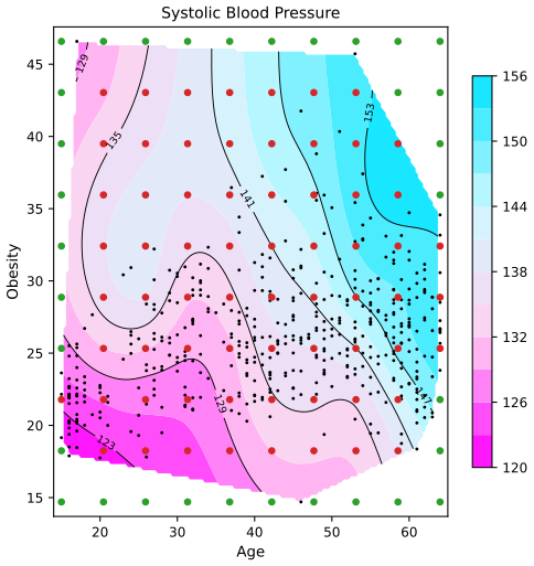
fig_5_12, class ThinPlate. Reproduces Hastie, Tibshirani and Friedman (2009), Figure 5.12. Download: PDF · SVGMore generally one can use any large basis in \(\R^d\) (for instance all tensor products of univariate B-splines) with a penalty such as (5.38), reducing the number of functions per coordinate as \(d\) grows. Additive models restrict the class: with
\[ J[f]=J(f_1+f_2+\dots+f_d)=\sum_{j=1}^d\int f_j''(t_j)^2\d t_j \tag{5.40} \]each \(f_j\) is a univariate smoothing spline (Chapter 9), and the ANOVA decomposition
\[ f(X)=\alpha+\sum_jf_j(X_j)+\sum_{j\lt k}f_{jk}(X_j,X_k)+\cdots \tag{5.41} \]adds interactions of chosen orders, each represented by regression splines and their tensor products or by complete bases with their own penalties. With many inputs, automatic methods (MARS, Chapter 9; boosted trees, Chapter 10) make these choices.
5.8 Regularization and Reproducing Kernel Hilbert Spaces
pp. 167–168 A general class of regularisation problems is
\[ \min_{f\in\Hc}\Big[\sum_{i=1}^NL(y_i,f(x_i))+\lambda J(f)\Big] \tag{5.42} \]with a loss \(L\), a penalty functional \(J\) and a space \(\Hc\) on which \(J\) is defined. Girosi et al. (1995) consider penalties of the form
\[ J(f)=\int_{\R^d}\frac{|\tilde f(s)|^2}{\tilde G(s)}\,\d s, \tag{5.43} \]with \(\tilde f\) the Fourier transform of \(f\) and \(\tilde G\gt0\) decaying as \(\|s\|\to\infty\), so high frequencies are penalised heavily. Under further conditions the solution has the form
\[ f(X)=\sum_{k=1}^K\alpha_k\phi_k(X)+\sum_{i=1}^N\theta_iG(X-x_i), \tag{5.44} \]where the \(\phi_k\) span the null space of \(J\) and \(G\) is the inverse Fourier transform of \(\tilde G\). Smoothing splines (\(\tilde G(s)\propto s^{-4}\) in one dimension) and thin-plate splines are of this type. The striking fact is again that an infinite-dimensional problem has a finite-dimensional solution.
5.8.1 Spaces of Functions Generated by Kernels
pp. 168–170 Let \(K(x,y)\) be a positive definite kernel on \(\R^p\) with eigen-expansion
\[ K(x,y)=\sum_{i=1}^\infty\gamma_i\phi_i(x)\phi_i(y) \tag{5.45} \](\(\gamma_i\ge0\), \(\phi_i\) orthonormal in \(L^2\)). The book requires \(\sum\gamma_i^2\lt\infty\); for the expansion to converge on the diagonal, \(K(x,x)=\sum_i\gamma_i\phi_i(x)^2\lt\infty\), which for a continuous kernel on a compact set (Mercer's theorem) comes with \(\sum_i\gamma_i=\int K(x,x)\d x\lt\infty\), a stronger condition.
Definition 5.4 (the RKHS \(\Hc_K\)) pp. 168–169, (5.46)–(5.47)
\(\Hc_K\) consists of the functions
\[ f(x)=\sum_{i=1}^\infty c_i\phi_i(x) \tag{5.46} \]with
\[ \|f\|_{\Hc_K}^2\stackrel{\rm def}{=}\sum_{i=1}^\infty c_i^2/\gamma_i\lt\infty, \tag{5.47} \]and inner product \(\langle f,g\rangle_{\Hc_K}=\sum_ic_id_i/\gamma_i\) for \(g=\sum_id_i\phi_i\) (terms with \(\gamma_i=0\) are excluded, i.e. such \(c_i\) must be 0). The penalty is \(J(f)=\|f\|^2_{\Hc_K}\): a generalised ridge penalty that charges little for directions with large \(\gamma_i\).
The problem (5.42) becomes
\[ \min_{f\in\Hc_K}\Big[\sum_{i=1}^NL(y_i,f(x_i))+\lambda\|f\|^2_{\Hc_K}\Big] \tag{5.48} \] \[ \min_{\{c_j\}_1^\infty}\Big[\sum_{i=1}^NL\Big(y_i,\sum_{j=1}^\infty c_j\phi_j(x_i)\Big)+\lambda\sum_{j=1}^\infty c_j^2/\gamma_j\Big]. \tag{5.49} \]Result 5.12 (the reproducing property; Exercise 5.15(a)–(c)) p. 169
For every \(x_i\), \(K(\cdot,x_i)\in\Hc_K\), and for \(f\in\Hc_K\)
\[ \langle K(\cdot,x_i),f\rangle_{\Hc_K}=f(x_i),\qquad \langle K(\cdot,x_i),K(\cdot,x_j)\rangle_{\Hc_K}=K(x_i,x_j). \]Hence for \(g=\sum_{i=1}^N\alpha_iK(\cdot,x_i)\),
\[ J(g)=\sum_{i=1}^N\sum_{j=1}^NK(x_i,x_j)\alpha_i\alpha_j=\bal^\T\bK\bal. \tag{5.51} \]Proof
By (5.45), \(K(\cdot,x_i)=\sum_k\{\gamma_k\phi_k(x_i)\}\phi_k\), so its coefficients are \(c_k=\gamma_k\phi_k(x_i)\) and \[\sum_kc_k^2/\gamma_k=\sum_k\gamma_k\phi_k(x_i)^2=K(x_i,x_i)\lt\infty\]: it belongs to \(\Hc_K\). For \(f=\sum_kc_k\phi_k\), \[\langle K(\cdot,x_i),f\rangle=\sum_k\gamma_k\phi_k(x_i)c_k/\gamma_k=\sum_kc_k\phi_k(x_i)=f(x_i)\] (a). Taking \(f=K(\cdot,x_j)\) gives (b). By bilinearity, \[\|g\|^2=\sum_{i,j}\alpha_i\alpha_j\langle K(\cdot,x_i),K(\cdot,x_j)\rangle=\sum_{i,j}\alpha_i\alpha_jK(x_i,x_j)\] (c). Because of (a), \(h_i=K(\cdot,x_i)\) is called the representer of evaluation at \(x_i\). ∎
Result 5.13 (the representer theorem; Exercise 5.15(d)) p. 169, (5.50), (5.52), (5.74)
Let \(g=\sum_{i=1}^N\alpha_iK(\cdot,x_i)\) and \(\tilde g=g+\rho\) with \(\rho\in\Hc_K\) orthogonal to every \(K(\cdot,x_i)\). Then
\[ \sum_{i=1}^NL(y_i,\tilde g(x_i))+\lambda J(\tilde g)\ \ge\ \sum_{i=1}^NL(y_i,g(x_i))+\lambda J(g), \tag{5.74} \]with equality iff \(\rho=0\) (for \(\lambda\gt0\)). Hence any solution of (5.48) has the finite form
\[ f(x)=\sum_{i=1}^N\alpha_iK(x,x_i), \tag{5.50} \]and (5.48) reduces to the \(N\)-dimensional problem
\[ \min_\bal\ L(\y,\bK\bal)+\lambda\bal^\T\bK\bal. \tag{5.52} \]Proof
By the reproducing property, \(\rho(x_i)=\langle K(\cdot,x_i),\rho\rangle=0\), so \(\tilde g(x_i)=g(x_i)\) and the loss terms are equal. By orthogonality, \[J(\tilde g)=\|g\|^2+2\langle g,\rho\rangle+\|\rho\|^2=J(g)+\|\rho\|^2\ge J(g)\], with equality iff \(\rho=0\). Now any \(f\in\Hc_K\) decomposes as \(f=g+\rho\), \(g\) the orthogonal projection of \(f\) onto the finite-dimensional (hence closed) subspace \(\operatorname{span}\{K(\cdot,x_i)\}\) and \(\rho\) orthogonal to it; so replacing \(f\) by \(g\) never increases the criterion, and strictly decreases it unless \(f=g\). The values at the data are \(g(x_j)=\sum_i\alpha_iK(x_j,x_i)=(\bK\bal)_j\), and \(J(g)=\bal^\T\bK\bal\) by (5.51), which gives (5.52). (Confirmed numerically for a Gaussian kernel: random components orthogonal to the representers vanish at the data and always raise the criterion.) ∎
This reduction from infinitely many to \(N\) parameters is the "kernel property" exploited by support vector machines (Chapter 12). Bayesian view. If \(f\) is a zero-mean Gaussian process with covariance \(K\), the eigenfunctions \(\phi_j\) have prior variances \(\gamma_j\); the penalty \(\sum c_j^2/\gamma_j\) is minus twice the log prior, so (5.48) with squared-error loss is a posterior mode, and the solution (5.57) below is the posterior mean of Gaussian-process regression (kriging), with \(\lambda\) the noise-to-signal variance ratio. Unpenalised components. When part of the space should not be penalised (the linear functions of the cubic smoothing spline, the plane of the thin-plate spline), write \(\Hc=\Hc_0\oplus\Hc_1\) and penalise \(\|P_1f\|^2\); the same argument gives \[f(x)=\sum_{j=1}^M\beta_jh_j(x)+\sum_{i=1}^N\alpha_iK(x,x_i)\] with \(h_j\) spanning \(\Hc_0\) (in the Bayesian view, a flat prior on the \(\Hc_0\) part).
See also (companion course): valid kernels and the reproducing-kernel construction, a representer theorem (Exercise 6.16) and Gaussian processes for regression; demonstrations: kernel functions, GP regression.
5.8.2 Examples of RKHS
pp. 170–174 Squared-error loss. (5.48) is then a penalised least-squares problem, in two equivalent forms:
\[ \min_{\{c_j\}_1^\infty}\sum_{i=1}^N\Big(y_i-\sum_{j=1}^\infty c_j\phi_j(x_i)\Big)^2+\lambda\sum_{j=1}^\infty\frac{c_j^2}{\gamma_j} \tag{5.53} \] \[ \min_\bal(\y-\bK\bal)^\T(\y-\bK\bal)+\lambda\bal^\T\bK\bal. \tag{5.54} \] \[ \hat\bal=(\bK+\lambda\bI)^{-1}\y, \tag{5.55} \] \[ \hat f(x)=\sum_{j=1}^N\hat\alpha_jK(x,x_j), \tag{5.56} \] \[ \hat\bff=\bK\hat\bal=\bK(\bK+\lambda\bI)^{-1}\y \tag{5.57} \] \[ \phantom{\hat\bff}=(\bI+\lambda\bK^{-1})^{-1}\y. \tag{5.58} \]Filling the gap 5.10: from (5.54) to (5.55) and (5.58) p. 171
Derivation
The gradient of (5.54) is \[-2\bK(\y-\bK\bal)+2\lambda\bK\bal=-2\bK\{\y-(\bK+\lambda\bI)\bal\}\]. It vanishes at \(\hat\bal=(\bK+\lambda\bI)^{-1}\y\) (invertible for \(\lambda\gt0\) since \(\bK\succeq0\)); if \(\bK\) is singular other minimisers differ by null vectors of \(\bK\), which change neither \(\bK\bal\) nor the penalty, so the fitted function is unique. When \(\bK\) is invertible, \[\bK(\bK+\lambda\bI)^{-1}=\{(\bK+\lambda\bI)\bK^{-1}\}^{-1}=(\bI+\lambda\bK^{-1})^{-1}\], the same form as the Reinsch formula (5.17) with \(\bK^{-1}\) in place of the spline penalty matrix. ∎
Penalised polynomial regression. The kernel \(K(x,y)=(\langle x,y\rangle+1)^d\) (Vapnik 1996) on \(\R^p\) has \(M=\binom{p+d}{d}\) eigenfunctions spanning the polynomials of total degree \(\le d\) (Filling the gap 5.1). For \(p=d=2\), \(M=6\) and
\[ K(x,y)=1+2x_1y_1+2x_2y_2+x_1^2y_1^2+x_2^2y_2^2+2x_1x_2y_1y_2 \tag{5.59} \] \[ \phantom{K(x,y)}=\sum_{m=1}^Mh_m(x)h_m(y) \tag{5.60} \] \[ h(x)^\T=(1,\sqrt2x_1,\sqrt2x_2,x_1^2,x_2^2,\sqrt2x_1x_2). \tag{5.61} \]In terms of the \(M\) orthonormal eigenfunctions and eigenvalues of \(K\),
\[ h(x)=\bV\bD_\gamma^{1/2}\phi(x), \tag{5.62} \]with \(\bD_\gamma=\diag(\gamma_1,\dots,\gamma_M)\) and \(\bV\) orthogonal (Exercise 5.16), and the ridge problem
\[ \min_{\{\beta_m\}_1^M}\sum_{i=1}^N\Big(y_i-\sum_{m=1}^M\beta_mh_m(x_i)\Big)^2+\lambda\sum_{m=1}^M\beta_m^2 \tag{5.63} \]is of the form (5.53). By (5.55), the kernel route needs \(N^2\) kernel evaluations and \(O(N^3)\) operations however large \(M\) is. But the penalty acts on the scaled features (5.61): the \(\sqrt2\) factors and the implied eigenvalues decide which polynomial directions are shrunk most.
Gaussian radial basis functions. With \(K(x,y)=e^{-\nu\|x-y\|^2}\) and squared-error loss the fit is an expansion in
\[ k_m(x)=e^{-\nu\|x-x_m\|^2},\qquad m=1,\dots,N, \tag{5.64} \]one radial function centred at each training point, with coefficients from (5.54).
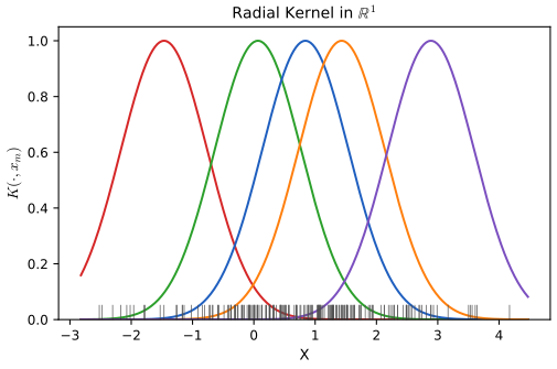
fig_5_13. Reproduces Hastie, Tibshirani and Friedman (2009), Figure 5.13. Download: PDF · SVGThe \(200\times200\) kernel matrix has eigen-decomposition \(\bK=\bPhi\bD_\gamma\bPhi^\T\). Its columns and eigenvalues estimate the eigenfunctions and eigenvalues of (5.45); the eigenvectors can be turned into functions on \(\R\) by the Nyström extension \(\hat\phi_\ell(x)=\hat\gamma_\ell^{-1}\sum_iK(x,x_i)\Phi_{i\ell}\), which returns \(\Phi_{i\ell}\) at \(x=x_i\) because \(\bK\bPhi_{\cdot\ell}=\hat\gamma_\ell\bPhi_{\cdot\ell}\) (Exercise 5.17). The feature-space functions
\[ h_\ell(x)=\sqrt{\hat\gamma_\ell}\,\hat\phi_\ell(x),\qquad\ell=1,\dots,N, \tag{5.65} \]satisfy \(\langle h(x_i),h(x_{i'})\rangle=K(x_i,x_{i'})\), and kernel ridge regression is ordinary ridge regression on them.
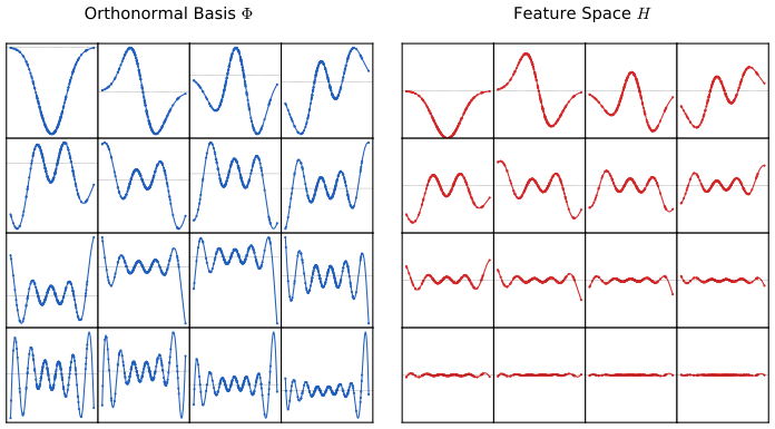
fig_5_14, nystrom. Reproduces Hastie, Tibshirani and Friedman (2009), Figure 5.14. Download: PDF · SVG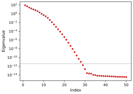
fig_5_15. Reproduces Hastie, Tibshirani and Friedman (2009), Figure 5.15. Download: PDF · SVGA thin-plate spline (Section 5.7) is also an expansion in radial functions, generated by
\[ K(x,y)=\|x-y\|^2\log(\|x-y\|), \tag{5.66} \]which is only conditionally positive definite; that is why the constraints of Result 5.11 and the unpenalised plane are needed.
Support vector classifiers. The support vector machine for \(y_i\in\{-1,1\}\) uses \(f(x)=\alpha_0+\sum_i\alpha_iK(x,x_i)\) with
\[ \min_{\alpha_0,\bal}\Big\{\sum_{i=1}^N[1-y_if(x_i)]_++\frac\lambda2\bal^\T\bK\bal\Big\}, \tag{5.67} \]a hinge loss plus the RKHS penalty; by Result 5.13 this form loses nothing. The problem is a quadratic program, and the flat part of the hinge makes many \(\hat\alpha_i=0\): only the "support vectors" enter \(\hat f\) (Section 12.3.3).
See also (companion course): maximum margin classifiers.
5.9 Wavelet Smoothing
pp. 174–176 Regression splines select a few basis functions; smoothing splines keep a complete basis and shrink toward smoothness. Wavelets keep a complete orthonormal basis and shrink and select toward a sparse representation: a mostly flat function with a few bumps needs only a few bumpy basis functions. Wavelets are localised both in time and in frequency, whereas Fourier functions are localised in frequency only.
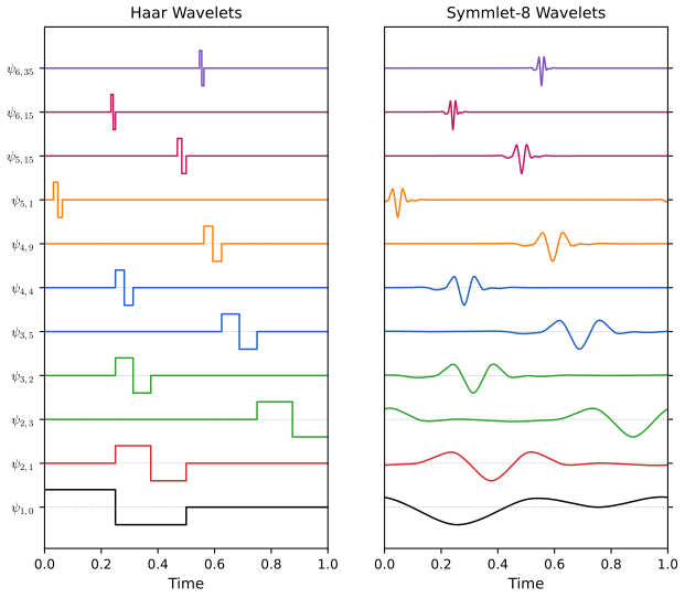
fig_5_16, wavelet_vector. Reproduces Hastie, Tibshirani and Friedman (2009), Figure 5.16. Download: PDF · SVGWavelet smoothing fits the coefficients of the full basis by least squares, then thresholds (discards) the small ones; with many functions at each scale it keeps detail only where it is needed.
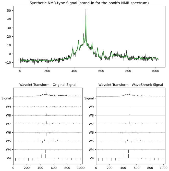
fig_5_17, wavelet_shrink. Reproduces Hastie, Tibshirani and Friedman (2009), Figure 5.17, with a substitute signal. Download: PDF · SVG5.9.1 Wavelet Bases and the Wavelet Transform
pp. 176–179 Wavelet bases are generated by translations and dilations of a scaling function (father wavelet) \(\phi\). For Haar, \(\phi(x)=I(x\in[0,1])\); \(\phi_{0,k}(x)=\phi(x-k)\) is an orthonormal basis of the space \(V_0\) of functions constant on the intervals \([k,k+1)\), and \(\phi_{j,k}(x)=2^{j/2}\phi(2^jx-k)\) spans \(V_j\), the functions constant on intervals of length \(2^{-j}\): \(\dots\subset V_{-1}\subset V_0\subset V_1\subset\dots\). As in analysis of variance, where two means are replaced by their average and a contrast, write \(V_{j+1}=V_j\oplus W_j\) with \(W_j\) the orthogonal complement (the detail), and set small contrasts to zero. For Haar the mother wavelet is \(\psi(x)=\phi(2x)-\phi(2x-1)\) and \(\psi_{j,k}=2^{j/2}\psi(2^jx-k)\).
Result 5.14 (the Haar multiresolution basis) pp. 176–178
(a) \(\{\psi_{j,k}\}_k\) is an orthonormal basis of \(W_j\). (b) \(V_J=V_0\oplus W_0\oplus W_1\oplus\dots\oplus W_{J-1}\), and \(\{\phi_{0,k}\}\cup\{\psi_{j,k}:0\le j\lt J\}\) is an orthonormal basis of \(V_J\). (c) On \(N=2^J\) equally spaced points of \([0,1)\) this gives \(1+\sum_{j=0}^{J-1}2^j=2^J=N\) orthonormal vectors, the columns of the wavelet matrix \(\bW\).
Proof
(a) For \(j=0\) (the others follow by the change of variable \(x\mapsto2^jx\), which preserves inner products up to the factor \(2^j\) absorbed in \(2^{j/2}\)). \(\psi(x-k)\) is \(+1\) on \([k,k+\tfrac12)\) and \(-1\) on \([k+\tfrac12,k+1)\), so \(\|\psi(\cdot-k)\|^2=1\), translates by different integers have disjoint supports, and \(\langle\psi(\cdot-k),\phi(\cdot-m)\rangle=\tfrac12-\tfrac12=0\) for \(m=k\) (and 0 otherwise): each \(\psi(\cdot-k)\in V_1\) is orthogonal to \(V_0\), i.e. lies in \(W_0\). Spanning: a function in \(V_1\) takes values \(a,b\) on the two halves of \([k,k+1)\); on that interval it equals \(\tfrac{a+b}2\phi(x-k)+\tfrac{a-b}2\psi(x-k)\), a \(V_0\) part plus a combination of the \(\psi(\cdot-k)\). So \(V_1=V_0\oplus\operatorname{span}\{\psi(\cdot-k)\}\) and the span is all of \(W_0\).
(b) Iterate \(V_{j+1}=V_j\oplus W_j\) from \(j=J-1\) down to 0. The spaces \(V_0,W_0,\dots,W_{J-1}\) are mutually orthogonal (\(W_j\perp V_j\supseteq V_{j'}\oplus W_{j'}\) for \(j'\lt j\)), so the union of orthonormal bases is orthonormal. (c) On \([0,1)\), \(V_0\) is the constants (one function) and \(W_j\) has the \(2^j\) translates \(k=0,\dots,2^j-1\). ∎
Haar functions are too rough for most purposes. Daubechies' symmlet-\(p\) wavelets are smoother; the price is a longer support (\(2p-1\) consecutive intervals; 15 for symmlet-8) and the gain is \(p\) vanishing moments, \(\int\psi(x)x^j\d x=0\), \(j=0,\dots,p-1\). As a consequence, polynomials of degree \(\le p-1\) on the \(N=2^J\) points are reproduced exactly in \(V_0\) (Exercise 5.18): \(V_0\) plays the role of the null space of the spline penalty. (Haar has one vanishing moment; \(V_0\) reproduces constants.) The general construction is through the two-scale relations
\[ \phi(x)=\sum_{k\in\mathbb Z}h(k)\phi_{1,k}(x),\qquad \psi(x)=\sum_{k\in\mathbb Z}g(k)\phi_{1,k}(x),\qquad g(k)=(-1)^{1-k}h(1-k). \]Filling the gap 5.11: why \(g(k)=(-1)^{1-k}h(1-k)\), and how the symmlet filter is computed p. 179
Derivation
Orthonormality conditions. The \(\phi_{1,k}\) are orthonormal, so \(\langle\phi(\cdot-m),\phi\rangle=\sum_kh(k)h(k+2m)\) (the translate by \(m\) shifts the index by \(2m\)). Orthonormality of the \(\phi(\cdot-m)\) is therefore \(\sum_kh(k)h(k+2m)=\delta_{m0}\); integrating the two-scale relation gives \(\sum_kh(k)=\sqrt2\) (as \(\int\phi=1\)). Likewise \(\langle\psi,\phi(\cdot-m)\rangle=\sum_kg(k)h(k+2m)\). With \(g(k)=(-1)^{1-k}h(1-k)\), substitute \(k\to1-k-2m\) in the sum: \(\sum_k(-1)^{1-k}h(1-k)h(k+2m)\) becomes \[\sum_k(-1)^{k+2m}h(k+2m)h(1-k)=-\sum_k(-1)^{1-k}h(1-k)h(k+2m)\], so the sum equals its own negative and is zero: \(\psi\perp V_0\). The same substitution shows \[\sum_kg(k)g(k+2m)=\sum_kh(k)h(k+2m)=\delta_{m0}\]. (For Haar this formula gives \(-\psi\); the sign is a convention. Our code uses the equivalent \(g(k)=(-1)^{k+1}h(L-1-k)\), which differs by an even shift.)
Vanishing moments and spectral factorisation. With \(m_0(\omega)=2^{-1/2}\sum_kh(k)e^{-ik\omega}\), the orthonormality conditions are \(|m_0(\omega)|^2+|m_0(\omega+\pi)|^2=1\), and \(p\) vanishing moments of \(\psi\) mean a zero of order \(p\) of \(m_0\) at \(\omega=\pi\). Daubechies' solution is \(|m_0(\omega)|^2=\cos^{2p}(\omega/2)\,P(\sin^2(\omega/2))\) with \(P(y)=\sum_{k=0}^{p-1}\binom{p-1+k}{k}y^k\), the polynomial of degree \(p-1\) with \((1-y)^pP(y)+y^pP(1-y)=1\). To recover \(h\), each root of \(P\) yields a pair of reciprocal roots \(z,1/z\) of the corresponding Laurent polynomial in \(z=e^{-i\omega}\); keeping one of each pair (complex pairs together, so that \(h\) is real) gives a valid filter. Keeping all roots inside the unit circle gives Daubechies' extremal-phase wavelets; the symmlets keep the combination whose phase is closest to linear (most nearly symmetric). For \(p=8\) we search the 16 admissible combinations; the result equals the standard symmlet-8 filter to \(10^{-12}\), satisfies \(\sum h=\sqrt2\) and the even-shift orthonormality to \(10^{-12}\), and \(g\) has exactly eight vanishing moments. ∎
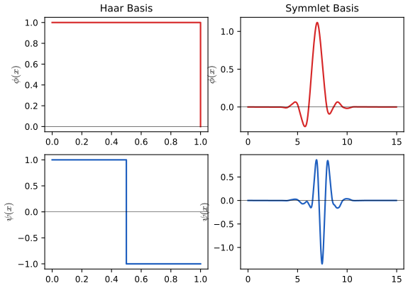
fig_5_18, cascade, daubechies_filter. Reproduces Hastie, Tibshirani and Friedman (2009), Figure 5.18. Download: PDF · SVG5.9.2 Adaptive Wavelet Filtering
pp. 179–181 Take \(N=2^J\) observations on a regular grid and let \(\bW\) be the \(N\times N\) orthonormal wavelet matrix. Then \(\y^*=\bW^\T\y\) is the wavelet transform of \(\y\) (and the full least-squares coefficient vector). SURE shrinkage (Donoho and Johnstone 1994) starts from the lasso criterion
\[ \min_\bth\|\y-\bW\bth\|_2^2+2\lambda\|\bth\|_1, \tag{5.68} \]whose solution is
\[ \hat\theta_j=\sgn(y_j^*)(|y_j^*|-\lambda)_+. \tag{5.69} \]Result 5.15 (in an orthonormal basis the lasso is soft thresholding) p. 179
If \(\bW^\T\bW=\bI\), the unique minimiser of (5.68) is (5.69), and \(\hat\bff=\bW\hat\bth\).
Proof
\(\bW\) is square and orthogonal, so \[\|\y-\bW\bth\|^2=\|\bW^\T\y-\bth\|^2=\sum_j(y_j^*-\theta_j)^2\], and (5.68) separates into \(N\) problems \(\min_\theta\,(y^*-\theta)^2+2\lambda|\theta|\). Each is strictly convex. For \(\theta\ne0\) the derivative is \(2(\theta-y^*)+2\lambda\sgn\theta\), zero at \(\theta=y^*-\lambda\sgn\theta\), consistent only if \(|y^*|\gt\lambda\) (then \(\theta=\sgn(y^*)(|y^*|-\lambda)\)). Otherwise the minimum is at 0, where the subdifferential \(2(0-y^*)+2\lambda[-1,1]\) contains 0 iff \(|y^*|\le\lambda\). Together: (5.69). ∎
See also (companion courses): the same soft-thresholding rule as the coordinate update of the lasso, Section 9.2.2, and the demonstration L1 versus L2 paths.
The universal threshold. A simple choice is \(\lambda=\sigma\sqrt{2\log N}\), with \(\sigma\) an estimate of the noise standard deviation (we use the median absolute deviation of the finest-level coefficients divided by 0.6745). The motivation: if \(\y\) is white noise, so is \(\y^*\) (orthonormal transformation), and the largest of \(N\) white-noise values is about \(\sigma\sqrt{2\log N}\), so coefficients below that are probably noise.
Filling the gap 5.12: the maximum of \(N\) Gaussian noise values p. 180
Derivation
Let \(Z_1,\dots,Z_N\sim N(0,\sigma^2)\) (not necessarily independent) and \(M=\max_j|Z_j|\). For \(t\gt0\), Jensen's inequality and \(e^{t|z|}\le e^{tz}+e^{-tz}\) give
\[ e^{t\E M}\le\E e^{tM}\le\sum_j\E\big(e^{tZ_j}+e^{-tZ_j}\big)=2Ne^{t^2\sigma^2/2}, \]so \(\E M\le\frac{\log(2N)}t+\frac{t\sigma^2}2\); the choice \(t=\sqrt{2\log(2N)}/\sigma\) gives \(\E M\le\sigma\sqrt{2\log(2N)}\). For independent variables a matching lower bound holds, \(\E M/(\sigma\sqrt{2\log N})\to1\), so \(\sigma\sqrt{2\log N}\) is the right order. Convergence is slow: for \(N=1024\), \(\sqrt{2\log N}=3.72\) and a simulation gives \(\Pr(M\lt3.72\sigma)\approx0.82\), so a pure-noise signal keeps on average a fraction of a coefficient. ∎
Result 5.16 (Stein's unbiased risk estimate for soft thresholding) p. 179 (SURE, in brief)
Let \(\bx\sim N(\bth,\bI_n)\) (coefficients of one level divided by \(\sigma\)) and \(\hat\bth_t=\) soft thresholding of \(\bx\) at \(t\). Then
\[ \E\|\hat\bth_t-\bth\|^2=\E\,\mathrm{SURE}(t;\bx),\qquad \mathrm{SURE}(t;\bx)=n-2\,\#\{i:|x_i|\le t\}+\sum_{i=1}^n\min(|x_i|,t)^2 . \]Proof
Stein's lemma. For \(X\sim N(\theta,1)\) and \(g\) absolutely continuous with \(\E|g'(X)|\lt\infty\), \(\E[(X-\theta)g(X)]=\E[g'(X)]\): integrate by parts, using \(\varphi'(x-\theta)=-(x-\theta)\varphi(x-\theta)\) for the normal density \(\varphi\). Risk. Write \(\hat\theta_i=x_i+g(x_i)\) with \(g(x)=-\sgn(x)\min(|x|,t)\). Then \[\E(\hat\theta_i-\theta_i)^2=\E(x_i-\theta_i)^2+2\E[(x_i-\theta_i)g(x_i)]+\E g(x_i)^2=1+2\E g'(x_i)+\E\min(|x_i|,t)^2\]. Since \(g'(x)=-I(|x|\lt t)\) almost everywhere, summing over \(i\) gives the formula; the quantity inside the expectation depends only on the data. SureShrink picks, at each level, the \(t\in[0,\sqrt{2\log n}]\) minimising SURE, falling back to the universal threshold when the level looks too sparse for SURE to be reliable. (Confirmed by simulation: average risk 38.65 against average SURE 38.82 over 4000 replications.) ∎
In Figure 5.17 the transform stops at \(V_4\) (16 scaling coefficients, never thresholded); the remaining columns of \(\bW\) are the \(\psi_{j,k}\), \(j=4,\dots,9\) for our \(N=1024\) (the book's signal has \(N=2048\), up to \(j=11\)). Coefficients shrink as the level rises, except where the signal has spikes. Comparing (5.68) with the smoothing-spline criterion (5.21):
- both are hierarchical from coarse to fine, but wavelets are also localised in time within each level;
- splines shrink each component by its own factor \(\rho_k\) (a built-in preference for smoothness), while basic SURE shrinkage treats all scales alike (level-dependent thresholds are a refinement);
- the spline's \(L_2\) penalty only shrinks; the \(L_1\) penalty shrinks and selects. Splines compress by smoothness, wavelets by sparsity.
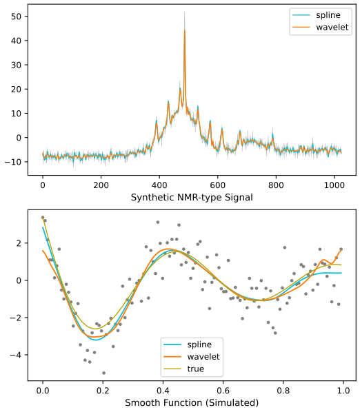
fig_5_19. Reproduces Hastie, Tibshirani and Friedman (2009), Figure 5.19, with a substitute signal in the top panel. Download: PDF · SVGThe transform is not computed by multiplying with \(\bW\): the pyramid algorithm filters and downsamples level by level in \(O(N)\) operations (faster than the FFT's \(O(N\log N)\)), and so does the inverse (Exercise 5.19). Our implementation agrees with an established wavelet library to \(10^{-10}\).
Appendix: Computations for Splines
B-splines
pp. 186–189 Add boundary knots \(\xi_0\lt\xi_1\) and \(\xi_K\lt\xi_{K+1}\) and form the augmented sequence \(\tau\): \(\tau_1\le\dots\le\tau_M\le\xi_0\); \(\tau_{j+M}=\xi_j\), \(j=1,\dots,K\); \(\xi_{K+1}\le\tau_{K+M+1}\le\dots\le\tau_{K+2M}\) (customarily all extra knots equal \(\xi_0\) and \(\xi_{K+1}\)). The B-splines of order \(m\le M\) are
\[ B_{i,1}(x)=\begin{cases}1&\text{if }\tau_i\le x\lt\tau_{i+1}\\0&\text{otherwise}\end{cases},\qquad i=1,\dots,K+2M-1, \tag{5.77} \] \[ B_{i,m}(x)=\frac{x-\tau_i}{\tau_{i+m-1}-\tau_i}B_{i,m-1}(x)+\frac{\tau_{i+m}-x}{\tau_{i+m}-\tau_{i+1}}B_{i+1,m-1}(x),\qquad i=1,\dots,K+2M-m, \tag{5.78} \]with the convention that a term with a zero denominator is 0 (so \(B_{i,m}=0\) when \(\tau_i=\dots=\tau_{i+m}\)). For \(M=4\), \(B_{i,4}\), \(i=1,\dots,K+4\), are the cubic B-splines; for \(m\lt M\) only \(B_{i,m}\), \(i=M-m+1,\dots,M+K\), are needed. At the right end we close the last non-empty interval, so that the basis is also correct at \(x=\xi_{K+1}\).
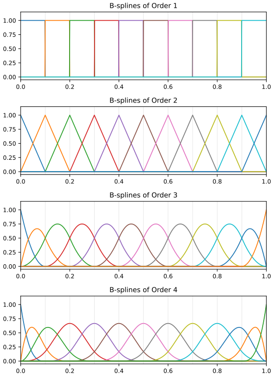
fig_5_20, bspline_basis (equal to an established library's B-spline design matrix to \(10^{-12}\)). Reproduces Hastie, Tibshirani and Friedman (2009), Figure 5.20. Download: PDF · SVGResult 5.17 (properties of B-splines; Exercise 5.2) p. 186
(a) \(B_{i,m}(x)=0\) for \(x\notin[\tau_i,\tau_{i+m}]\). (b) \(B_{i,m}(x)\gt0\) for \(x\in(\tau_i,\tau_{i+m})\) (when \(\tau_i\lt\tau_{i+m}\)). (c) \(\sum_iB_{i,M}(x)=1\) on \([\xi_0,\xi_{K+1}]\). (d) \(B_{i,M}\) is a piecewise polynomial of degree \(M-1\) with breaks only at the knots, and the \(K+M\) functions are a basis of the order-\(M\) splines. (e) For equally spaced simple knots \(0,1,\dots,M\), \(B_{1,M}\) is the density of \(U_1+\dots+U_M\), \(U_j\) independent \(U(0,1)\).
Proof
(a), (b) by induction on \(m\): true for \(m=1\). If they hold for order \(m-1\), the two terms of (5.78) vanish outside \([\tau_i,\tau_{i+m-1}]\) and \([\tau_{i+1},\tau_{i+m}]\), so \(B_{i,m}\) vanishes outside their union \([\tau_i,\tau_{i+m}]\). Inside, the weights \((x-\tau_i)/(\tau_{i+m-1}-\tau_i)\) and \((\tau_{i+m}-x)/(\tau_{i+m}-\tau_{i+1})\) are positive where their B-splines are, and at every interior point at least one of the two lower-order splines is positive.
(c) By induction: \[\sum_iB_{i,m}(x)=\sum_i\Big[\frac{x-\tau_i}{\tau_{i+m-1}-\tau_i}+\frac{\tau_{i+m-1}-x}{\tau_{i+m-1}-\tau_i}\Big]B_{i,m-1}(x)=\sum_iB_{i,m-1}(x)\], after shifting the index in the second sum (\(i+1\to i\)); the end terms vanish because the corresponding B-splines are zero on \([\xi_0,\xi_{K+1}]\). So the sum is \(\sum_iB_{i,1}=1\).
(d) Each step of (5.78) multiplies piecewise polynomials by linear functions, raising the degree by one, with breaks only at the \(\tau\)'s; so \(B_{i,M}\) is piecewise of degree \(M-1\), with breaks at the knots. The smoothness \(C^{M-2}\) at a simple knot follows from the derivative formula \(B'_{i,m}=(m-1)\big[\frac{B_{i,m-1}}{\tau_{i+m-1}-\tau_i}-\frac{B_{i+1,m-1}}{\tau_{i+m}-\tau_{i+1}}\big]\) by induction (if order \(m-1\) is \(C^{m-3}\), the derivative of order \(m\) is \(C^{m-3}\), so the function is \(C^{m-2}\)). That the \(K+M\) functions are independent (hence a basis of the \((M+K)\)-dimensional space of Result 5.2) uses the local support: on the first interval only \(M\) of them are non-zero and they restrict to independent polynomials, and so on interval by interval (de Boor 1978).
(e) The density of \(U_1\) is \(B_{1,1}\) with knots 0, 1. If \(f_{m-1}=B_{1,m-1}\) (knots \(0,\dots,m-1\)), the density of \(S_m=S_{m-1}+U_m\) is \(f_m(x)=\int_{x-1}^xf_{m-1}(s)\d s\). With equally spaced knots, (5.78) and the derivative formula give \[B'_{1,m}(x)=B_{1,m-1}(x)-B_{1,m-1}(x-1)\], which is also \(f_m'\); both vanish at 0, so \(f_m=B_{1,m}\). Equivalently, both equal \(\frac1{(m-1)!}\sum_{k=0}^m(-1)^k\binom mk(x-k)_+^{m-1}\) (the Irwin–Hall density), confirmed numerically to \(10^{-12}\). ∎
Repeated knots. If an interior knot \(\xi_j\) appears \(r_j\) times (\(1\le r_j\le M\)) the lowest discontinuous derivative at \(\xi_j\) has order \(M-r_j\): a triple knot in a cubic gives a kink, a quadruple knot a jump. The boundary knots are repeated \(M\) times, which is why the B-spline basis is "discontinuous" there, i.e. undefined beyond the boundary.
Computations for Smoothing Splines
pp. 189–190 Least squares with \(K+M\) basis functions costs \(O(N(K+M)^2+(K+M)^3)\), i.e. \(O(N^3)\) when \(K\) is a fraction of \(N\). Sorted data and local support fix this. Writing \(f(x)=\sum_{j=1}^{N+4}\gamma_jB_j(x)\) with cubic B-splines on the \(N\) distinct inputs,
\[ \hat\bgam=(\bB^\T\bB+\lambda\bOm_B)^{-1}\bB^\T\y, \tag{5.79} \]with \(\bB\) the \(N\times(N+4)\) basis matrix and \(\{\bOm_B\}_{jk}=\int B_j''B_k''\). \(\bB\) is 4-banded (each row has at most four non-zeros), so \(\bB^\T\bB+\lambda\bOm_B\) is banded with bandwidth 4, its Cholesky factor is banded, and the solve costs \(O(N)\).
Filling the gap 5.13: why the unconstrained B-spline fit is the natural spline p. 189
Explanation
The book says the penalty "automatically imposes" the natural boundary conditions. Here is the precise statement. Let \(\mathcal S\) be the cubic splines on \([a,b]\) with knots at the data, \(a\le x_1\), \(x_N\le b\), and penalty \(\int_a^bf''^2\). The natural spline \(g\) of Result 5.5 belongs to \(\mathcal S\) (restricted to \([a,b]\)) and minimises the criterion over all functions; so it minimises it over \(\mathcal S\), and the minimiser over \(\mathcal S\) is unique (same argument). Hence the B-spline solution is linear on \([a,x_1]\) and \([x_N,b]\) and has \(g''(x_1)=g''(x_N)=0\), although no constraint was imposed: these are the natural boundary conditions of the variational problem, and any curvature beyond the data would cost penalty without improving the fit. Confirmed numerically: with the \(N+2\) B-splines of Exercise 5.8 the fitted values agree with the Reinsch algorithm to \(10^{-9}\). For large \(N\) not all knots are needed; R's smooth.spline thins them roughly logarithmically (all knots for \(N\lt50\), only 204 for \(N=5000\)) with negligible effect on the fit. ∎
Exercises
Each exercise is restated in my own words, followed by a complete solution. Exercises that need computation give the method and the result of the chapter code.
Exercise 5.1. Show that the six functions (5.3) are a basis of the cubic splines with knots \(\xi_1,\xi_2\).
Solution
This is Result 5.2 with \(M=4\), \(K=2\): each function is a cubic spline (the truncated cubics have continuous first and second derivatives at their knot), every cubic spline \(f\) equals \(p_0+\theta_1(X-\xi_1)_+^3+\theta_2(X-\xi_2)_+^3\) where \(p_0\) is its leftmost cubic piece and \(\theta_\ell\) one sixth of the jump of \(f'''\) at \(\xi_\ell\) (the difference of two adjacent pieces has a triple zero at the knot, hence is a multiple of \((X-\xi_\ell)^3\)), and the six functions are independent (restrict to the first interval, then the second, then the third). So the space is 6-dimensional, as the count \(3\times4-2\times3\) predicts. Numerically, the basis (5.3) and the cubic B-splines give identical least-squares fits and their combined columns have rank 7 for three knots.
Exercise 5.2. For the B-splines (5.77)–(5.78) show: (a) \(B_{i,M}(x)=0\) outside \([\tau_i,\tau_{i+M}]\) (so a cubic B-spline spans at most 5 knots); (b) \(B_{i,M}\gt0\) on \((\tau_i,\tau_{i+M})\); (c) \(\sum_{i=1}^{K+M}B_{i,M}(x)=1\) on \([\xi_0,\xi_{K+1}]\); (d) \(B_{i,M}\) is a piecewise polynomial of order \(M\) with breaks only at the knots; (e) an order-\(M\) B-spline is the density of a convolution of \(M\) uniform random variables.
Solution
All five parts are proved in Result 5.17, by induction on the order through (5.78) and the derivative formula. For (e) the statement is exact for equally spaced simple knots: the cardinal B-spline is the Irwin–Hall density of \(U_1+\dots+U_M\). For general knots the normalised B-spline \(\frac{M}{\tau_{i+M}-\tau_i}B_{i,M}\) is still a probability density, that of \(\sum_{j=0}^M\tau_{i+j}D_j\) with \((D_0,\dots,D_M)\) uniformly distributed on the simplex (the Curry–Schoenberg theorem); for equally spaced knots this reduces to the sum of uniforms. Numerically, a histogram of \(2\times10^5\) sums of three uniforms matches \(B_{1,3}\) to 0.02, and the closed forms agree to \(10^{-12}\).
Exercise 5.3. Write a program to reproduce Figure 5.3.
Solution
See
fig_5_3andpointwise_variancein the chapter code and Figure 5.3. Method: draw 50 inputs from \(U[0,1]\); build the four basis matrices (linear; cubic; truncated power basis (5.3) with knots 0.33, 0.66; natural spline basis (5.4)–(5.5) with knots 0.1, 0.26, 0.42, 0.58, 0.74, 0.9); evaluate \(\bh(x)^\T(\bH^\T\bH)^{-1}\bh(x)\) on a grid. Check: the values at the 50 inputs sum to 2, 4, 6 and 6 (Filling the gap 5.4).Exercise 5.4. For the truncated power representation (5.70) of a cubic spline with \(K\) knots, show that the natural boundary conditions are equivalent to \(\beta_2=\beta_3=0\), \(\sum_k\theta_k=0\), \(\sum_k\xi_k\theta_k=0\) (5.71), and derive the basis (5.4)–(5.5).
Solution
See the proof of Result 5.3. A more constructive derivation of (5.4)–(5.5): solve the two \(\bth\)-constraints for \(\theta_{K-1},\theta_K\). From \(\sum\theta_k=0\) and \(\sum\xi_k\theta_k=0\): \(\theta_K=\sum_{k\le K-2}\theta_k\frac{\xi_{K-1}-\xi_k}{\xi_K-\xi_{K-1}}\) and \(\theta_{K-1}=-\sum_{k\le K-2}\theta_k\frac{\xi_K-\xi_k}{\xi_K-\xi_{K-1}}\). Substituting, the truncated part becomes \[\sum_{k\le K-2}\theta_k(\xi_K-\xi_k)\{d_k(X)-d_{K-1}(X)\}\], and with \(\beta_2=\beta_3=0\) the spline is \(\beta_0+\beta_1X+\sum_{k\le K-2}\tilde\theta_kN_{k+2}(X)\), \(\tilde\theta_k=\theta_k(\xi_K-\xi_k)\). (Expand \(d_k-d_{K-1}\) to check: its coefficient of \((X-\xi_K)_+^3\) is \(\frac{-1}{\xi_K-\xi_k}+\frac{1}{\xi_K-\xi_{K-1}}\), matching.) Numerically, a random natural spline refitted in the truncated power basis has \(\beta_2,\beta_3,\sum\theta_k,\sum\xi_k\theta_k\) all below \(10^{-8}\).
Exercise 5.5. Classify the phoneme data with quadratic discriminant analysis after filtering the correlated features with a smooth natural cubic spline basis (Section 5.2.3). Fix five choices of the number and position of knots in advance and choose among them by tenfold cross-validation.
Solution
Method (
exercise_5_5): the "aa"/"ao" frames with the same 1000/717 training/test split as Figure 5.5; filtered features \(x^*=\bH^\T x\) with \(\bH\) the \(256\times M\) natural-spline basis (knots including the two boundary knots at frequencies 1 and 256); QDA with class means, unbiased class covariances and class priors from the training data; tenfold CV on the training set; the chosen basis is refitted on the whole training set and evaluated once on the test set.Knots (fixed in advance) 10-fold CV error Test error \(M=4\), uniform 0.256 0.273 \(M=8\), uniform 0.217 0.209 \(M=12\), uniform 0.193 0.190 \(M=20\), uniform 0.217 0.194 \(M=12\), log-spaced (denser at low frequency) 0.198 0.188 CV selects 12 uniformly spaced knots; its test error, 0.190, is close to that of the restricted logistic regression (0.187) and far better than QDA on the 256 raw features (0.381), where each class covariance has 32 896 parameters estimated from about 400 to 600 frames. Too few knots (4) lose the low-frequency structure; too many (20) bring back variance. Log-spaced knots, which follow the observation that low frequencies discriminate, do about as well.
Exercise 5.6. How would you modify the truncated power basis to fit a periodic function with known period \(T\)?
Solution
Map the input to \([0,T)\) by \(u=X\bmod T\) and require the fitted cubic spline to join smoothly across \(u=0\equiv T\). With the truncated power basis on \([0,T)\), \(f(u)=\sum_{j=0}^3\beta_ju^j+\sum_k\theta_k(u-\xi_k)_+^3\), add the linear constraints \(f^{(r)}(0)=f^{(r)}(T^-)\) for \(r=0,1,2\) (and \(r=3\) too unless 0 is itself a knot, since the third derivative may only jump at knots); with \(K\) knots in \((0,T)\) the \(K+4\) coefficients and 4 constraints leave \(K\) free parameters, the dimension of the periodic cubic splines with \(K\) knots on a circle (\(K\) pieces, \(4K-3K\)). Fit by least squares under these constraints, or eliminate them. A ready-made basis: use \(1\) and the periodised Bernoulli quartics \(b_k(X)=B_4\big(((X-\xi_k)\bmod T)/T\big)\), \(B_4(t)=t^4-2t^3+t^2-\tfrac1{30}\), with \(\sum_kc_k=0\). Each \(b_k\) is \(T\)-periodic and twice continuously differentiable (\(B_4\), \(B_4'\), \(B_4''\) take equal values at 0 and 1), its third derivative jumps only at \(\xi_k\), and the constraint cancels the quartic terms, leaving a piecewise cubic. This is a \(K\)-dimensional space (confirmed numerically, together with periodicity and the \(C^2\) property). A periodic smoothing spline is obtained in the same way, with the penalty integrated over one period.
Exercise 5.7 (Green and Silverman 1994). Let \(g\) be the natural cubic spline interpolating \((x_i,z_i)\), \(a\lt x_1\lt\dots\lt x_N\lt b\), \(N\ge2\), and \(\tilde g\) any other differentiable interpolant on \([a,b]\). (a) With \(h=\tilde g-g\), show \[\int_a^bg''h''=-\sum_{j=1}^{N-1}g'''(x_j^+)\{h(x_{j+1})-h(x_j)\}=0\] (5.72). (b) Hence \(\int\tilde g''^2\ge\int g''^2\), with equality only if \(h\equiv0\). (c) Deduce that the minimiser of the penalised least-squares criterion is a cubic spline with knots at the \(x_i\).
Solution
All three parts are Steps 1–3 of the proof of Result 5.5; the sum is zero because \(h\) vanishes at every data point. Two remarks: \(\tilde g\) must have \(\tilde g'\) absolutely continuous and \(\tilde g''\) square-integrable for the integrals to make sense (merely differentiable is not enough), and the minimiser in (c) is not just a cubic spline but a natural one (linear outside \([x_1,x_N]\)). Numerically, for 25 points the natural interpolant has \(\int g''^2\) smaller than the not-a-knot cubic interpolant, and random perturbations of the smoothing-spline values always increase the criterion.
Exercise 5.8. The Appendix computes smoothing splines with \(N+4\) B-splines. Describe a slightly simpler scheme with an \((N+2)\)-dimensional B-spline basis on the \(N-2\) interior knots.
Solution
Take the boundary knots \(\xi_0=x_1\), \(\xi_{K+1}=x_N\) and the interior knots \(x_2,\dots,x_{N-1}\) (\(K=N-2\)): the cubic B-splines number \(K+4=N+2\) and span the cubic splines on \([x_1,x_N]\) with knots at all data points. Compute \(\bB\) (\(N\times(N+2)\), at most four non-zeros per row) and \(\bOm_B=\int_{x_1}^{x_N}B_j''B_k''\) exactly (the \(B_j''\) are piecewise linear: two- or three-point Gauss–Legendre quadrature on each knot interval is exact), then solve the banded system \((\bB^\T\bB+\lambda\bOm_B)\bgam=\bB^\T\y\) by banded Cholesky in \(O(N)\). The solution is the natural smoothing spline on \([x_1,x_N]\) (Filling the gap 5.13): the natural boundary conditions come out of the optimisation; outside \([x_1,x_N]\) extend linearly. Our implementation (
smoothing_spline_bspline) agrees with the Reinsch algorithm to \(10^{-9}\).Exercise 5.9. Derive the Reinsch form \(\bS_\lambda=(\bI+\lambda\bK)^{-1}\).
Solution
See Result 5.6. In brief: \(\bN\) (natural spline basis with knots at the \(N\) distinct inputs, evaluated there) is invertible, so put \(\bK=\bN^{-\T}\bOm_N\bN^{-1}\), which does not involve \(\lambda\). Then \[\bS_\lambda=\bN(\bN^\T\bN+\lambda\bOm_N)^{-1}\bN^\T=\bN\{\bN^\T(\bI+\lambda\bK)\bN\}^{-1}\bN^\T=(\bI+\lambda\bK)^{-1}\]. The explicit form \(\bK=\bQ\bR^{-1}\bQ^\T\) is derived in the same result; the two agree numerically.
Exercise 5.10. Derive expressions for \(\var\hat f_\lambda(x_0)\) and \(\Bias\hat f_\lambda(x_0)\). Using (5.22), make a version of Figure 5.9 showing the mean and several pointwise quantiles of \(\hat f_\lambda(x)\).
Solution
See Result 5.8: \(\hat f_\lambda(x_0)=\bl(x_0)^\T\y\), \(\var=\sigma^2\|\bl(x_0)\|^2\), \(\Bias=f(x_0)-\bl(x_0)^\T\bff\), and with Gaussian errors the distribution is exactly normal, so the quantiles are \(\bl^\T\bff\pm z_q\sigma\|\bl\|\). The weights are computed by evaluating, at \(x_0\), the natural splines that interpolate the columns of \(\bS_\lambda\) (
operator_at). Figure 5.S1 shows the mean and the 50%, 80% and 95% bands for 5, 9 and 15 df. A simulation with 2000 replications gives coverage 0.79–0.81 for the 80% bands at four points.Exercise 5.11. Prove that the null space of \(\bK\) for a smoothing spline is spanned by functions linear in \(X\).
Solution
See Result 5.7(a): \(\bg^\T\bK\bg=\int g''^2\) for the natural spline \(g\) with values \(\bg\), so \(\bK\bg=\mathbf0\iff\bg^\T\bK\bg=0\) (\(\bK\succeq0\)) \(\iff g''\equiv0\iff g\) is linear \(\iff\bg\in\operatorname{span}\{\mathbf1,\bx\}\). Numerically \(\bK[\mathbf1,\bx]=\mathbf0\) to rounding and \(\rank\bK=N-2\).
Exercise 5.12. Characterise the minimiser of the weighted criterion \(\sum_iw_i\{y_i-f(x_i)\}^2+\lambda\int\{f''(t)\}^2\d t\) (5.73), \(w_i\ge0\). Characterise the smoothing spline when there are ties in \(X\).
Solution
See Result 5.10(c). If at least two distinct inputs have positive weight, the minimiser is unique and is the natural cubic spline with knots at the distinct inputs with positive weight (points with \(w_i=0\) do not influence the fit; they are evaluated on the spline), with fitted values \(\hat\bff=(\bW+\lambda\bK)^{-1}\bW\y\). Ties: for the distinct values \(t_1\lt\dots\lt t_n\) with counts \(n_j\) (or summed weights) and mean responses \(\bar y_j\), \[\sum_{i:x_i=t_j}(y_i-f(t_j))^2=n_j(\bar y_j-f(t_j))^2+\sum(y_i-\bar y_j)^2\], so the smoothing spline is the weighted spline on the \(t_j\) with weights \(n_j\) and responses \(\bar y_j\): knots at the distinct values only, at most \(n\) degrees of freedom. The leave-one-out formula (5.27) remains valid with \(S_{ii}=w_i[(\bW+\lambda\bK)^{-1}]_{jj}\) (confirmed numerically against explicit refits).
Exercise 5.13. After fitting \(\hat f_\lambda\) to \(N\) pairs, add the pair \((x_0,\hat f_\lambda(x_0))\) and refit. Describe the result, and use it to derive the leave-one-out formula.
Solution
The refit is identical to \(\hat f_\lambda\) (for any \(x_0\), new or tied); the leave-one-out formula (5.27) follows by linearity. Full proof: Result 5.9. Numerically, the refit differs from the original by less than \(10^{-10}\), and (5.27) equals \(N\) explicit refits to \(10^{-10}\).
Exercise 5.14. Derive the constraints on the \(\alpha_j\) in the thin-plate expansion (5.39) that make the penalty finite. How else could finiteness be ensured?
Solution
\(\sum_j\alpha_j=0\) and \(\sum_j\alpha_jx_j=\mathbf0\) (three linear constraints in two dimensions), and then \(J=8\pi\bal^\T\bE\bal\): proof in Result 5.11. Without the constraints the integrand grows like \((\log r)^2\) or decays only like \(r^{-2}\) at infinity. Alternatives: compute the penalty over a bounded domain only (e.g. a rectangle or the convex hull of the data), which makes it finite for any coefficients but changes the optimal basis; or use radial functions with decaying second derivatives (e.g. Gaussian), giving an RKHS penalty as in Section 5.8. Numerically, the integral of (5.38) over a large square equals \(8\pi\bal^\T\bE\bal\) to 0.05% under the constraints, and grows with the domain when \(\sum\alpha_j\ne0\).
Exercise 5.15. For \(K\) satisfying (5.45) and \(f\in\Hc_K\), show (a) \(\langle K(\cdot,x_i),f\rangle_{\Hc_K}=f(x_i)\); (b) \(\langle K(\cdot,x_i),K(\cdot,x_j)\rangle_{\Hc_K}=K(x_i,x_j)\); (c) \(J(g)=\sum_{i,j}K(x_i,x_j)\alpha_i\alpha_j\) for \(g=\sum_i\alpha_iK(\cdot,x_i)\); (d) for \(\tilde g=g+\rho\) with \(\rho\in\Hc_K\) orthogonal to every \(K(\cdot,x_i)\), the inequality (5.74), with equality iff \(\rho=0\).
Solution
(a)–(c): Result 5.12; (d): Result 5.13 (for \(\lambda\gt0\); with \(\lambda=0\) equality holds for every \(\rho\)). The key step in (d) is that \(\rho\) vanishes at every data point by the reproducing property, while the penalty adds \(\|\rho\|^2\).
Exercise 5.16. Consider the ridge problem (5.53) with \(M\ge N\) and a kernel computing \(K(x,y)=\sum_{m=1}^Mh_m(x)h_m(y)\). (a) Derive (5.62); how are \(\bV\) and \(\bD_\gamma\) computed from \(K\)? Show that (5.63) is equivalent to (5.53). (b) Show \(\hat\bff=\bH\hat\bbeta=\bK(\bK+\lambda\bI)^{-1}\y\) (5.75), with \(\bH\) the \(N\times M\) matrix \(h_m(x_i)\) and \(\bK=\bH\bH^\T\). (c) Show \(\hat f(x)=h(x)^\T\hat\bbeta=\sum_iK(x,x_i)\hat\alpha_i\) (5.76), \(\hat\bal=(\bK+\lambda\bI)^{-1}\y\). (d) What changes if \(M\lt N\)?
Solution
(a) Let \(\mu\) be the measure defining the \(L^2\) inner product and \(\mathbf G=\int h(x)h(x)^\T\d\mu(x)\) (\(M\times M\), positive definite if the \(h_m\) are independent). The integral operator of \(K\) maps \(\phi=\mathbf a^\T h\) to \(\int K(\cdot,y)\phi(y)\d\mu(y)=h^\T\mathbf G\mathbf a\), so its eigenfunctions are \(\phi=\mathbf a^\T h\) with \(\mathbf G\mathbf a=\gamma\mathbf a\) and \(\mathbf a^\T\mathbf G\mathbf a=1\). With the eigen-decomposition \(\mathbf G=\bV\bD_\gamma\bV^\T\), take \(\mathbf a_\ell=\bV_{\cdot\ell}\gamma_\ell^{-1/2}\): \(\phi(x)=\bD_\gamma^{-1/2}\bV^\T h(x)\), i.e. \(h(x)=\bV\bD_\gamma^{1/2}\phi(x)\) (5.62). So \(\bV,\bD_\gamma\) come from the eigen-decomposition of the Gram matrix of the features (in practice estimated by \(\frac1N\bH^\T\bH\), which has the same non-zero eigenvalues as \(\frac1N\bK\)). Substituting, \[\sum_m\beta_mh_m(x)=\bbeta^\T\bV\bD_\gamma^{1/2}\phi(x)=\sum_\ell c_\ell\phi_\ell(x)\] with \(\mathbf c=\bD_\gamma^{1/2}\bV^\T\bbeta\), and \(\|\bbeta\|^2=\|\bV^\T\bbeta\|^2=\sum_\ell c_\ell^2/\gamma_\ell\): (5.63) is (5.53) with finitely many terms.
(b) \[\hat\bbeta=(\bH^\T\bH+\lambda\bI_M)^{-1}\bH^\T\y=\bH^\T(\bH\bH^\T+\lambda\bI_N)^{-1}\y\] by the push-through identity \((\bH^\T\bH+\lambda\bI)\bH^\T=\bH^\T(\bH\bH^\T+\lambda\bI)\). Hence \(\hat\bff=\bH\hat\bbeta=\bK(\bK+\lambda\bI)^{-1}\y\).
(c) \[\hat f(x)=h(x)^\T\hat\bbeta=h(x)^\T\bH^\T\hat\bal=\sum_ih(x)^\T h(x_i)\hat\alpha_i=\sum_iK(x,x_i)\hat\alpha_i\] with \(\hat\bal=(\bK+\lambda\bI)^{-1}\y\). Confirmed numerically for the kernel (5.59): the six-feature ridge and the kernel solution agree at the data and at new points.
(d) Nothing in (b)–(c) needs \(M\ge N\): the identities hold for any \(M\). With \(M\lt N\), however, \(\bK=\bH\bH^\T\) has rank at most \(M\lt N\), so it is singular: (5.58) is unavailable, \(\hat\bal\) is still well defined by \((\bK+\lambda\bI)^{-1}\y\), and it is cheaper to solve the \(M\times M\) primal system \((\bH^\T\bH+\lambda\bI)\bbeta=\bH^\T\y\) at \(O(NM^2+M^3)\) instead of \(O(N^3)\).
Exercise 5.17. Show how to turn the discrete eigen-decomposition of \(\bK\) in Section 5.8.2 into estimates of the eigenfunctions of \(K\).
Solution
The eigenfunctions satisfy \(\int K(x,y)\phi(y)p(y)\d y=\gamma\phi(x)\) for the input density \(p\). Replace the integral by the average over the sample: \(\frac1N\sum_iK(x,x_i)\phi(x_i)=\gamma\phi(x)\). At \(x=x_j\) this is the matrix eigenproblem \(\bK\mathbf v=N\gamma\mathbf v\) with \(\mathbf v=(\phi(x_i))_i\); so \(\hat\gamma_\ell=\gamma_\ell(\bK)/N\) and \(\hat\phi_\ell(x_i)=\sqrt N\,\Phi_{i\ell}\) (normalised so that \(\frac1N\sum_i\hat\phi_\ell(x_i)^2=1\)). For other \(x\), use the same equation as a definition (the Nyström extension): \[\hat\phi_\ell(x)=\frac{1}{N\hat\gamma_\ell}\sum_iK(x,x_i)\hat\phi_\ell(x_i)=\frac{\sqrt N}{\gamma_\ell(\bK)}\sum_iK(x,x_i)\Phi_{i\ell}\], a smooth function that reproduces the eigenvector at the data points exactly (confirmed numerically). This is how Figure 5.14 draws the eigenvectors as functions; it is reliable while \(\gamma_\ell(\bK)\) is well above rounding level.
Exercise 5.18. The symmlet-\(p\) wavelet \(\psi\) has \(p\) vanishing moments. Show that polynomials of order \(p\) are then represented exactly in \(V_0\).
Solution
Let \(q\) be a polynomial of degree \(\le p-1\) (order \(p\)). For every \(j\ge0\) and \(k\), \[\langle q,\psi_{j,k}\rangle=2^{j/2}\int q(x)\psi(2^jx-k)\d x=2^{-j/2}\int q\big(2^{-j}(u+k)\big)\psi(u)\d u=0\], because \(q(2^{-j}(u+k))\) is a polynomial in \(u\) of degree \(\le p-1\) and \(\psi\) annihilates all of those. So \(q\) has no component in any \(W_j\), \(j\ge0\). Since \(V_J=V_0\oplus W_0\oplus\dots\oplus W_{J-1}\) and the restriction of \(q\) to the sampled grid lies in \(V_J\), it lies in \(V_0\). On a finite grid the statement holds for the wavelets whose support does not straddle the ends (with periodic wrap-around the polynomial has a jump at the boundary). Numerically: for a degree-7 polynomial on 1024 points the symmlet-8 detail coefficients away from the ends are below \(10^{-14}\), while the eighth moment of the high-pass filter is non-zero, so degree 8 is not reproduced. This makes \(V_0\) the analogue of the null space (the linear functions) of the cubic smoothing-spline penalty.
Exercise 5.19. Show that the Haar wavelet transform of a signal of length \(N=2^J\) can be computed in \(O(N)\) operations.
Solution
Pyramid algorithm. Set \(a^{(J)}=\y\). For \(j=J-1,\dots,0\) compute, for \(k=0,\dots,2^j-1\), \(a^{(j)}_k=(a^{(j+1)}_{2k}+a^{(j+1)}_{2k+1})/\sqrt2\) and \(d^{(j)}_k=(a^{(j+1)}_{2k}-a^{(j+1)}_{2k+1})/\sqrt2\). These are the inner products of the signal with \(\phi_{j,k}\) and \(\pm\psi_{j,k}\) (the two-scale relations with \(h=(1,1)/\sqrt2\)). Level \(j\) costs \(2\cdot2^j\) additions/subtractions and as many multiplications by \(1/\sqrt2\); summing, \(2(2^{J-1}+\dots+1)=2(N-1)\) additions, i.e. \(O(N)\). The output \(\{a^{(0)},d^{(0)},\dots,d^{(J-1)}\}\) is \(\bW^\T\y\). The inverse runs the steps backwards, \(a^{(j+1)}_{2k}=(a^{(j)}_k+d^{(j)}_k)/\sqrt2\), \(a^{(j+1)}_{2k+1}=(a^{(j)}_k-d^{(j)}_k)/\sqrt2\), also \(O(N)\). For a filter of length \(L\) (16 for symmlet-8) the cost is \(O(LN)\).
Demonstrations for this chapter
Each demonstration runs in the browser on the book's data (or on the signals described), and links back to these notes. The ▶ Demo boxes above open them already set to the case under discussion.
| Demonstration | What you can see | Sections and results |
|---|---|---|
| Regression splines with movable knots | Piecewise constant, linear, quadratic and cubic splines and natural cubic splines on artificial data or data from (5.22); drag the knots; truncated power versus B-spline basis (same fit, different conditioning); standard-error bands. Presets: 1 piecewise constant; 2 continuous piecewise linear; 3 cubic spline; 4 natural cubic spline; 5 conditioning. | 5.2, 5.2.1, Appendix; Results 5.2, 5.3, 5.17 |
| Smoothing splines: df and the eigenvalues of the smoother | Ozone, bone density and simulated data; a df slider; the eigenvalues \(\rho_k(\lambda)\) against a projection smoother; any eigenvector and its shrunken version; the leave-one-out CV and GCV curves. Presets: 1 ozone 5 df; 2 ozone 11 df; 3 bone 12 df; 4 CV choice on (5.22); 5 over-fitting. | 5.4, 5.4.1, 5.5; Results 5.6, 5.7, 5.9 |
| Wavelet shrinkage of a noisy signal | Haar and symmlet-8 transforms of six signals; coefficients by level before and after thresholding; SURE, universal or manual thresholds; soft or hard; the coarsest level. Presets: 1 SureShrink; 2 universal threshold; 3 Haar on blocks; 4 Doppler; 5 hard thresholding. | 5.9; Results 5.14–5.16 |
Related demonstrations in the companion courses: basis functions and least squares, kernel functions, Gaussian-process regression and L1 versus L2 regularisation. The Python code for every figure on this page is code/ch05_basis_expansions.py (see the code index).
References
- Hastie, T., Tibshirani, R. and Friedman, J. (2009). The Elements of Statistical Learning: Data Mining, Inference, and Prediction, 2nd edition. Springer, New York. Chapter 5. hastie.su.domains/ElemStatLearn.
- Bachrach, L. K., Hastie, T., Wang, M.-C., Narasimhan, B. and Marcus, R. (1999). Bone mineral acquisition in healthy Asian, Hispanic, Black and Caucasian youth: a longitudinal study. Journal of Clinical Endocrinology and Metabolism, 84, 4702–4712.
- de Boor, C. (1978). A Practical Guide to Splines. Springer, New York.
- Daubechies, I. (1992). Ten Lectures on Wavelets. SIAM, Philadelphia.
- Donoho, D. L. and Johnstone, I. M. (1994). Ideal spatial adaptation by wavelet shrinkage. Biometrika, 81(3), 425–455. doi:10.1093/biomet/81.3.425.
- Donoho, D. L. and Johnstone, I. M. (1995). Adapting to unknown smoothness via wavelet shrinkage. Journal of the American Statistical Association, 90(432), 1200–1224.
- Evgeniou, T., Pontil, M. and Poggio, T. (2000). Regularization networks and support vector machines. Advances in Computational Mathematics, 13(1), 1–50.
- Girosi, F., Jones, M. and Poggio, T. (1995). Regularization theory and neural network architectures. Neural Computation, 7(2), 219–269.
- Green, P. J. and Silverman, B. W. (1994). Nonparametric Regression and Generalized Linear Models: A Roughness Penalty Approach. Chapman and Hall, London.
- Hastie, T. and Zhu, J. (2006). Discussion of "Support vector machines with applications" by J. Moguerza and A. Muñoz. Statistical Science, 21(3), 352–357.
- Kimeldorf, G. and Wahba, G. (1971). Some results on Tchebycheffian spline functions. Journal of Mathematical Analysis and Applications, 33(1), 82–95.
- Ramsay, J. O. and Silverman, B. W. (1997). Functional Data Analysis. Springer, New York.
- Reinsch, C. H. (1967). Smoothing by spline functions. Numerische Mathematik, 10, 177–183.
- Stein, C. M. (1981). Estimation of the mean of a multivariate normal distribution. Annals of Statistics, 9(6), 1135–1151.
- Vapnik, V. (1996). The Nature of Statistical Learning Theory. Springer, New York.
- Wahba, G. (1990). Spline Models for Observational Data. SIAM, Philadelphia.
The numerical statements in the text (Table 5.1, the equality of the different spline bases and smoothing-spline algorithms, the leave-one-out identity, the exact EPE values, the thin-plate penalty constant, the representer theorem, the wavelet filters and transforms, and the SURE identity) were confirmed numerically.