Discrete Latent Variables
A model can be made far more expressive by adding variables that are never observed. If each observation carries a hidden label saying which of \(K\) simple distributions produced it, the distribution of the observations alone is a mixture, and fitting it becomes a problem with missing data. This chapter starts from the simplest clustering method, K-means, recasts the Gaussian mixture as a latent-variable model, derives the expectation–maximization (EM) algorithm three times, each time more generally, and ends with the evidence lower bound (ELBO): the inequality \(\ln p(\bX\given\btheta)\ge\LB(q,\btheta)\) that later chapters use to train variational autoencoders and diffusion models.
Ch. 1 Deep learning revolution Ch. 2 Probabilities Ch. 3 Standard distributions Ch. 4 Regression Ch. 5 Classification Ch. 6 Deep neural networks Ch. 7 Gradient descent Ch. 8 Backpropagation Ch. 9 Regularization Ch. 10 Convolutional networks Ch. 11 Structured distributions Ch. 12 Transformers Ch. 13 Graph neural networks Ch. 14 Sampling Ch. 15 Discrete latent variables Ch. 16 Continuous latent variables Ch. 17 GANs Ch. 18 Normalizing flows Ch. 19 Autoencoders Ch. 20 Diffusion models Appendices A to C
How to read these notes
They follow the book. Sections carry the book's numbers (15.1, 15.3.2, ...) and every displayed equation that appears in the book carries the book's own equation number, e.g. (15.52). Equations without a number are steps that the book skips.
Filling the gaps. Wherever the book states a result without proof, says it "can be shown", or leaves it to an exercise, an orange Filling the gap box or a proof gives the full argument. Proofs start hidden: open one with its bar, or use the button below.
Figures and demonstrations. Twelve of the sixteen figures are reproduced by the Python code; the schematic ones (the bar diagrams 15.13–15.15 and the parameter-space sketch 15.16) are computed here from a real model. Figures 15.4, 15.9, 15.10 and 15.11 are graphical-model diagrams with no data and are not reproduced. Four supplementary figures (15.S1 to 15.S4, our own) illustrate gaps that are filled. The ▶ Demo boxes open an interactive demonstration already set to the case being discussed.
Main reference
C. M. Bishop and H. Bishop, Deep Learning: Foundations and Concepts, Springer (2024), Chapter 15, pages 459–493. Section, equation, figure and exercise numbers below refer to this book. Further reading is listed in the references; the book's website is www.bishopbook.com. There is no official solution for the exercises of this chapter; all solutions below are my own.
The explanations, derivations, figures and code are my own; equations are cited by their numbers in the book.
Companion course: Bayesian and Probabilistic Machine Learning
Sections 15.1 to 15.3 and most of 15.4 retell Chapter 9 of Bishop (2006), which the companion course Bayesian and Probabilistic Machine Learning covers in full. Where a result is the same, these notes state it with a short proof and link the complete derivation there. What this book presents differently gets the full treatment here: the ELBO written in the per-example form used for VAEs and diffusion models, EM as coordinate ascent on the ELBO with the exact size of each gain, the precise form of the K-means limit, the curvature of the bound (where the book says "convex"), the correspondence between local maxima, and vector quantisation in blocks.
- K-means, its convergence and its sequential form: Section 9.1, Result 9.1 (here 15.1); image segmentation and compression: Section 9.1.1 (here 15.1.1).
- Gaussian mixtures as latent-variable models, singularities, the likelihood equations and EM: Section 9.2, 9.2.1, 9.2.2 (here 15.2).
- The complete-data view, the K-means limit and Bernoulli mixtures: Section 9.3, 9.3.1, 9.3.2, 9.3.3 (here 15.3).
- The EM algorithm in general (decomposition, monotonicity, tangency, MAP, incremental EM): Section 9.4 (here 15.4); variational inference, where the same bound is maximised over a restricted family: Section 10.1; the ELBO in a variational autoencoder: Advanced topics, lecture 1; hidden Markov models: Section 13.2.
- Tools: Jensen's inequality, the Kullback–Leibler divergence, Lagrange multipliers, log-sum-exp.
- Demonstrations: K-means and EM step by step on Old Faithful and the EM bound with one free parameter. The three demonstrations of this chapter were chosen not to repeat them.
The chapter at a glance
- 15.1 K-means alternates two exact minimisations of the distortion \(J\), so \(J\) never increases and the algorithm stops after finitely many steps (Result 15.1). Used on pixels it segments and compresses images; on blocks of pixels it compresses far better at the same bit rate (Filling the gap 15.2).
- 15.2 A Gaussian mixture is the marginal of a model with a hidden 1-of-K label (Result 15.2). Its likelihood is unbounded (Result 15.3), has \(K!\) equivalent maxima (Result 15.4), and its stationarity conditions suggest EM (Result 15.5).
- 15.3 With the labels known, the likelihood is maximised in closed form; EM maximises its posterior expectation (Result 15.6). With covariances \(\epsilon\bI\) and \(\epsilon\to0\), EM becomes K-means: responsibilities harden exponentially fast and \(\epsilon Q\to-J/2\) (Result 15.7). Bernoulli mixtures learn digit prototypes without labels and have no singularities (Result 15.9).
- 15.4 For any \(q\), \(\ln p(\bX\given\btheta)=\LB(q,\btheta)+\KL(q\|p)\) (Result 15.10); EM is coordinate ascent on \(\LB\), and each M step raises the log likelihood by the rise of the bound plus a KL term (Result 15.11). The bound touches the log likelihood with the same slope and at least as much curvature (Result 15.12); for exponential families it is concave in the natural parameters, not convex (Result 15.13). Priors, partial steps and incremental updates all keep the monotonicity (Results 15.15–15.17), and the per-example form of the bound is the one VAEs maximise (Filling the gap 15.6).
Notation. \(\bX\) is the \(N\times D\) data matrix with rows \(\bx_n^\T\); \(\bZ\) the \(N\times K\) matrix of latent 1-of-K vectors \(\bz_n\); \(\gamma(z_{nk})=p(z_{nk}=1\given\bx_n,\btheta)\) the responsibilities; \(N_k=\sum_n\gamma(z_{nk})\); \(\btheta\) all parameters; \(Q(\btheta,\btheta^\old)\) the expected complete-data log likelihood; \(\LB(q,\btheta)\) the evidence lower bound. \(r_{nk}\in\{0,1\}\) are K-means assignments and \(J\) the distortion.
Printings. The first printing has a few slips in this chapter: the margin reference for \(\KL\ge0\), index typos in Algorithms 15.1 and 15.2, the dimension in (15.14), a missing factor in (15.33), "convex" where "concave" is meant on p. 488, and a normalisation of Bernoulli parameters that is not a constraint. Each is flagged where it occurs; the list with the evidence is in the summary before the exercises.
pp. 459–460 Chapter 11 built complicated distributions from simple ones with graphs. Here the extra ingredient is a latent (hidden) variable: a quantity that is part of the model but not of the data, such as the unknown orientation of an object in an image, or simply a label introduced to make the model richer. If \(p(\bx,\bz)\) is a joint distribution over observed \(\bx\) and latent \(\bz\), the model for the data is the marginal \(p(\bx)=\sum_\bz p(\bx,\bz)\). A tractable joint can have a very flexible marginal. With a discrete \(\bz\) the marginal is a mixture; this chapter studies that case, and Chapter 16 the continuous one.
15.1 K-means Clustering
See also the companion course, Section 9.1 (K-means clustering) and its K-means and EM demo.
pp. 460–461 Given \(N\) points \(\bx_1,\dots,\bx_N\in\R^D\) and a number \(K\) of clusters, we look for \(K\) prototypes \(\bmu_k\) and an assignment of each point to one of them so that points are close to their prototype.
Definition 15.1 (assignments and distortion) p. 460, (15.1)
Each point gets binary indicators \(r_{nk}\in\{0,1\}\) with \(\sum_kr_{nk}=1\) (the 1-of-K coding): \(r_{nk}=1\) when \(\bx_n\) is assigned to cluster \(k\). The distortion or error function is
\[ J=\sum_{n=1}^N\sum_{k=1}^Kr_{nk}\|\bx_n-\bmu_k\|^2 , \tag{15.1} \]the sum of squared distances of the points to their assigned prototypes.
K-means minimises \(J\) by alternating over the two groups of unknowns. With the prototypes fixed (the E step, so called because it will turn out to be the E step of EM), \(J\) is linear in the \(r_{nk}\) and separates over \(n\), so each point goes to its nearest prototype:
\[ r_{nk}=\begin{cases}1,&\text{if }k=\argmin_j\|\bx_n-\bmu_j\|^2,\\0,&\text{otherwise.}\end{cases} \tag{15.2} \]With the assignments fixed (the M step), \(J\) is a convex quadratic in each \(\bmu_k\); setting the gradient to zero,
\[ 2\sum_{n=1}^Nr_{nk}(\bx_n-\bmu_k)=\bzero , \tag{15.3} \] \[ \bmu_k=\frac{\sum_nr_{nk}\bx_n}{\sum_nr_{nk}} , \tag{15.4} \]the mean of the points in cluster \(k\), hence the name (Lloyd, 1982; MacQueen, 1967).
Algorithm 15.1 (K-means) p. 462
- Choose initial prototypes \(\bmu_1,\dots,\bmu_K\) (for example \(K\) distinct data points).
- E step: for every \(n\), set \(r_{nk}\) by (15.2), keeping the current label when there is a tie.
- M step: for every \(k\) with at least one point, set \(\bmu_k\) by (15.4); an empty cluster keeps its prototype.
- Repeat 2–3 until no assignment changes; return the \(\bmu_k\) and the \(r_{nk}\).
(The book's loop header reads "for \(N\in\{1,\dots,N\}\)"; the loop variable is \(n\).)
Result 15.1 (K-means never increases \(J\) and stops after finitely many steps) p. 461; Exercise 15.1
- The E step minimises \(J\) over all assignments for the current prototypes, and the M step minimises \(J\) over all prototypes for the current assignments, uniquely for every non-empty cluster: \(J(\bmu+\bdelta)-J(\bmu)=\sum_kN_k\|\bdelta_k\|^2\), where \(N_k\) is the size of cluster \(k\).
- Hence \(J\) is non-increasing, and with the tie rule of Algorithm 15.1 the algorithm stops after at most \(K^N\) cycles at an assignment that the E step leaves unchanged. The limit is a local minimum in the sense that neither step can improve it, not necessarily the global minimum.
Proof (short; the companion course has the same result as Result 9.1, and Exercise 15.1 below has the complete termination argument)
(1) \(J=\sum_n\big(\sum_kr_{nk}\|\bx_n-\bmu_k\|^2\big)\) and each bracket is smallest when its single 1 sits on the nearest prototype. For the M step, with \(\bar\bx_k\) the mean of cluster \(k\), \(\sum_{n\in k}\|\bx_n-\bar\bx_k-\bdelta_k\|^2\)
On the standardised Old Faithful data, from the starting centres of Figure 15.1, \(J\) takes the values 1048.40, 357.50, 170.87, 80.97, 79.91, 79.64, 79.61, 79.58 after the successive E and M steps and the fifth E step changes nothing (checked).
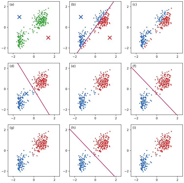
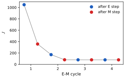
pp. 462–464 In practice the centres are started at \(K\) randomly chosen data points (or by the k-means++ rule of Arthur and Vassilvitskii (2007), used in our code), and K-means is often used to start EM for a Gaussian mixture. A sequential version updates only the nearest prototype as each point arrives:
\[ \bmu_k^\new=\bmu_k^\old+\frac1{N_k}(\bx_n-\bmu_k^\old) , \tag{15.5} \]where \(N_k\) counts the points used so far for \(\bmu_k\), including \(\bx_n\).
Filling the gap 15.1: the sequential update (15.5) is an exact running mean p. 464; Exercise 15.2
We show that (15.5) is not an approximation: after any sequence of updates each prototype is exactly the mean of the points that were assigned to it.
Derivation
Fix a cluster \(k\) and let \(\bx_{(1)},\dots,\bx_{(m)}\) be the points assigned to it so far, in order, with mean \(\bmu^{(m)}=\frac1m\sum_{i=1}^m\bx_{(i)}\). Separating the last point,
\[ \bmu^{(m)}=\frac{m-1}m\,\bmu^{(m-1)}+\frac1m\bx_{(m)}=\bmu^{(m-1)}+\frac1m\big(\bx_{(m)}-\bmu^{(m-1)}\big), \]which is (15.5) with \(N_k=m\). For \(m=1\) the step size is 1 and the prototype jumps onto the first point, so the starting value is forgotten. Induction on \(m\) gives the claim. Two remarks. (i) Each point is assigned using the prototypes current at the time it is seen; after the prototypes move, the nearest-prototype labelling of the earlier points may differ, so a single pass does not minimise \(J\). (ii) The step sizes \(1/N_k\) satisfy \(\sum1/m=\infty\) and \(\sum1/m^2<\infty\), the Robbins–Monro conditions, so (15.5) is also a stochastic-approximation scheme for a root of \(\partial J/\partial\bmu_k\) (companion course, Filling the gap 9.2). A numerical experiment runs one pass over Old Faithful in random order and finds each final prototype equal to the mean of its points to \(4\times10^{-16}\). ∎
p. 464 K-means makes hard assignments: a point midway between two centres is given entirely to one. The probabilistic treatment of Section 15.2 replaces them by soft assignments that express this uncertainty.
15.1.1 Image segmentation
See also the companion course, Section 9.1.1 (image segmentation and compression).
pp. 464–466 Treat every pixel of a colour image as a point in the space of its (R, G, B) intensities, run K-means, and redraw each pixel in the colour of its centre. The result is a segmentation into \(K\) colours that ignores where the pixels are (the space is not quite Euclidean either, since intensities lie in \([0,1]\), but this does not matter for K-means). The same construction is vector quantisation, a form of lossy compression: store the \(K\) codebook vectors \(\bmu_k\) and, for each pixel, only the index of its nearest one.
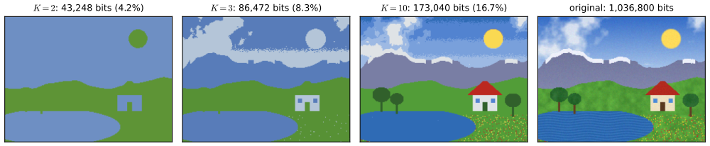
An image with \(N\) pixels stored at 8 bits per channel costs \(24N\) bits. The quantised version costs \(24K\) bits for the codebook plus \(\lceil\log_2K\rceil\) bits per pixel, \(24K+N\lceil\log_2K\rceil\) in all. For \(N=43{,}200\): 43,248, 86,472 and 173,040 bits for \(K=2\), 3, 10, that is 4.2%, 8.3% and 16.7% of the original 1,036,800 bits (all checked).
Filling the gap 15.2: the bit count, and why blocks of pixels compress better pp. 465–466
The book closes the section by remarking that a good compressor would quantise small blocks of adjacent pixels. We make this quantitative.
Derivation and experiment
The count. With \(K\) codewords, a fixed-length code needs \(b=\lceil\log_2K\rceil\) bits per index, since \(b\) bits distinguish \(2^b\ge K\) values; for \(K=3\) this is 2 bits, so a fourth colour would cost nothing extra per pixel. Each codeword has 3 numbers of 8 bits. Hence \(24K+N\lceil\log_2K\rceil\). (A variable-length code could lower the second term to about \(N\) times the entropy of the label frequencies, which is never more than \(\log_2K\).)
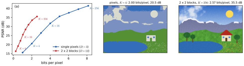
Blocks. Group the image into non-overlapping \(s\times s\) blocks, so each data vector has \(D=3s^2\) entries and there are \(N/s^2\) of them. The cost becomes \(24s^2K+(N/s^2)\lceil\log_2K\rceil\) bits. For \(s=2\) and \(K=128\) this is 2.034 bits per pixel, about the same as \(K=4\) single pixels (2.002). Why should blocks do better at the same rate? Neighbouring pixels are strongly correlated, so the 12-dimensional block vectors fill only a thin part of \([0,1]^{12}\); a codebook adapted to that part covers it with far fewer codewords than the product of four independent pixel codebooks would need. Vector quantisation of ever larger blocks can approach the best possible rate–distortion trade-off of the source (a classical result of information theory; Gersho and Gray, 1992), at the price of a codebook whose size grows exponentially with the rate times the block size.
Measured. Figure 15.S1 runs K-means on pixels and on 2 × 2 blocks of the test image for \(K=2,4,\dots,256\). At 2 bits per pixel, pixels reach 20.5 dB and blocks 33.5 dB; blocks at 2.6 bits per pixel (35.5 dB) nearly match pixels at 5.0 bits per pixel (35.6 dB, \(K=32\)). ∎
15.2 Mixtures of Gaussians
See also the companion course, Section 9.2, and Section 3.2.9 of these notes (mixtures of Gaussians).
pp. 466–467 Section 3.2.9 introduced the Gaussian mixture as a superposition
\[ p(\bx)=\sum_{k=1}^K\pi_k\N(\bx\given\bmu_k,\Sig_k). \tag{15.6} \]Definition 15.2 (the Gaussian mixture as a latent-variable model) pp. 466–467, (15.7)–(15.10)
Let \(\bz\) be a 1-of-K binary vector: \(z_k\in\{0,1\}\), \(\sum_kz_k=1\). Its distribution is \(p(z_k=1)=\pi_k\), where
\[ 0\le\pi_k\le1 \tag{15.7} \] \[ \sum_{k=1}^K\pi_k=1 , \tag{15.8} \]which, because exactly one \(z_k\) equals 1, can be written as
\[ p(\bz)=\prod_{k=1}^K\pi_k^{z_k}. \tag{15.9} \]Given \(z_k=1\), \(\bx\) is Gaussian, \(p(\bx\given z_k=1)=\N(\bx\given\bmu_k,\Sig_k)\), that is
\[ p(\bx\given\bz)=\prod_{k=1}^K\N(\bx\given\bmu_k,\Sig_k)^{z_k}. \tag{15.10} \]The joint is \(p(\bz)p(\bx\given\bz)\) (the two-node graph of Figure 15.4, not reproduced).
Result 15.2 (marginal and posterior of the latent-variable model) pp. 467–468, (15.11)–(15.12); Exercise 15.3
The marginal of \(\bx\) is the Gaussian mixture,
\[ p(\bx)=\sum_\bz p(\bz)p(\bx\given\bz)=\sum_{k=1}^K\pi_k\N(\bx\given\bmu_k,\Sig_k), \tag{15.11} \]and the posterior probability of component \(k\), the responsibility it takes for explaining \(\bx\), is
\[ \gamma(z_k)\equiv p(z_k=1\given\bx)=\frac{p(z_k=1)p(\bx\given z_k=1)}{\sum_{j=1}^Kp(z_j=1)p(\bx\given z_j=1)}=\frac{\pi_k\N(\bx\given\bmu_k,\Sig_k)}{\sum_{j=1}^K\pi_j\N(\bx\given\bmu_j,\Sig_j)}. \tag{15.12} \]Proof (short; the companion's Result 9.2 is the same)
\(\bz\) ranges over the \(K\) unit vectors \(\mathbf e_1,\dots,\mathbf e_K\). For \(\bz=\mathbf e_j\) every factor of (15.9) and (15.10) with \(k\ne j\) has exponent 0 and equals 1, so \(p(\mathbf e_j)p(\bx\given\mathbf e_j)=\pi_j\N(\bx\given\bmu_j,\Sig_j)\); summing over \(j\) gives (15.11). (15.12) is Bayes' theorem with this denominator. In code the responsibilities are a softmax of \(a_k=\ln\pi_k+\ln\N(\bx\given\bmu_k,\Sig_k)\) computed with log-sum-exp. ∎
Each observation \(\bx_n\) has its own latent \(\bz_n\). The latent form lets us work with the joint instead of the marginal, which is what makes EM possible. It also gives a sampler (ancestral sampling, Section 14.2.5): draw \(\widehat\bz\sim p(\bz)\), then \(\bx\sim p(\bx\given\widehat\bz)\).
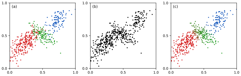
15.2.1 Likelihood function
See also the companion course, Section 9.2.1 (maximum likelihood) and Result 9.3.
pp. 468–470 For data \(\bX\) the log likelihood is
\[ \ln p(\bX\given\bpi,\bmu,\Sig)=\sum_{n=1}^N\ln\Big\{\sum_{k=1}^K\pi_k\N(\bx_n\given\bmu_k,\Sig_k)\Big\}. \tag{15.13} \]The sum inside the logarithm is what prevents a closed-form maximum. The likelihood also has two structural problems.
Result 15.3 (the mixture likelihood is unbounded; a single Gaussian's is not) pp. 469–470, (15.14), Figure 15.6
Let \(K\ge2\), \(\Sig_j=\sigma_j^2\bI\) and \(\bmu_j=\bx_n\) for some data point. Then the \(n\)th term of (15.13) contains
\[ \N(\bx_n\given\bx_n,\sigma_j^2\bI)=\frac1{(2\pi)^{D/2}}\frac1{\sigma_j^D}, \tag{15.14} \]and if another component \(k\) has fixed \(\pi_k>0\) and non-singular covariance, \(\ln p(\bX)\to+\infty\) as \(\sigma_j\to0\), growing like \(D\ln(1/\sigma_j)\). For a single Gaussian (\(K=1\)) the same collapse sends \(\ln p(\bX)\to-\infty\) unless all points coincide. (The book prints \((2\pi)^{-1/2}\sigma_j^{-1}\), the case \(D=1\).)
Proof (short; full version in the companion's Result 9.3)
Each term of (15.13) is at least \(\ln\{\pi_k\N(\bx_i\given\bmu_k,\Sig_k)\}\), a finite number independent of \(\sigma_j\); the \(n\)th term is also at least \(\ln\pi_j+\ln\N(\bx_n\given\bx_n,\sigma_j^2\bI)\)
A numerical experiment puts one component of a two-component mixture on an Old Faithful point: from \(\sigma_j=10^{-3}\) to \(10^{-6}\), \(\ln p\) rises by exactly \(2\ln10=4.61\) per decade (\(D=2\)).
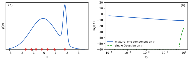
The singularities are a form of over-fitting. Remedies: detect a collapsing component and restart it with a random mean and a large covariance, or add a prior (Section 15.4.3). The second problem is symmetry.
Result 15.4 (\(K!\) equivalent solutions) p. 470; Exercise 15.4
Permuting the labels of the components, \((\pi_k,\bmu_k,\Sig_k)\mapsto(\pi_{\sigma(k)},\bmu_{\sigma(k)},\Sig_{\sigma(k)})\) for a permutation \(\sigma\) of \(\{1,\dots,K\}\), leaves the density (15.6), and so the likelihood, unchanged. If the \(K\) triples are distinct, the \(K!\) permutations give \(K!\) distinct parameter vectors. If some triples coincide, there are fewer: \(K!/\prod_jm_j!\) for groups of \(m_j\) equal components (and then a whole continuum, since equal components can share their total weight in any proportion).
Proof
A sum does not depend on the order of its terms. Two permutations \(\sigma\ne\sigma'\) give the same parameter vector exactly when \(\sigma'^{-1}\sigma\) only exchanges equal triples, so with distinct triples the map \(\sigma\mapsto\) parameter vector is injective on the \(K!\) permutations. With groups of sizes \(m_j\) of equal triples, permutations within a group fix the vector, and counting cosets gives \(K!/\prod_jm_j!\). That these are all parameter vectors giving the same density is the identifiability of finite Gaussian mixtures up to labels (Yakowitz and Spragins, 1968). A direct computation confirms the 6 permutations of a 3-component mixture give the same likelihood to \(10^{-9}\). ∎
Identifiability matters when the parameters are interpreted, not when the model is used as a density estimator.
15.2.2 Maximum likelihood
See also the companion course, Section 9.2.2 (EM for Gaussian mixtures) and Filling the gaps 9.5, 9.6 and 9.7.
pp. 470–472 The book gives three derivations of EM, each more general. The first only writes down the conditions for a maximum of (15.13).
Result 15.5 (the likelihood equations) pp. 471–472, (15.15)–(15.21)
At a stationary point of (15.13) with non-singular covariances,
\[ 0=\sum_{n=1}^N\underbrace{\frac{\pi_k\N(\bx_n\given\bmu_k,\Sig_k)}{\sum_j\pi_j\N(\bx_n\given\bmu_j,\Sig_j)}}_{\gamma(z_{nk})}\Sig_k^{-1}(\bx_n-\bmu_k) \tag{15.15} \]so that
\[ \bmu_k=\frac1{N_k}\sum_{n=1}^N\gamma(z_{nk})\bx_n \tag{15.16} \] \[ N_k=\sum_{n=1}^N\gamma(z_{nk}) ; \tag{15.17} \] \[ \Sig_k=\frac1{N_k}\sum_{n=1}^N\gamma(z_{nk})(\bx_n-\bmu_k)(\bx_n-\bmu_k)^\T ; \tag{15.18} \]and, maximising the Lagrangian
\[ \ln p(\bX\given\bpi,\bmu,\Sig)+\lambda\Big(\sum_{k=1}^K\pi_k-1\Big), \tag{15.19} \] \[ 0=\sum_{n=1}^N\frac{\N(\bx_n\given\bmu_k,\Sig_k)}{\sum_j\pi_j\N(\bx_n\given\bmu_j,\Sig_j)}+\lambda , \tag{15.20} \]with \(\lambda=-N\), hence
\[ \pi_k=\frac{N_k}N . \tag{15.21} \]These are not a closed-form solution, because the \(\gamma(z_{nk})\) depend on the parameters; they are a fixed-point system, and alternating "compute \(\gamma\)" and "solve for the parameters" is EM.
Proof (short; each step is written out in the companion's Filling the gaps 9.5–9.7)
Means. \(\partial_{\bmu_k}\ln\sum_j\pi_j\N_j\)
Covariances. With \(\ln\N\)
Weights. \(\partial_{\pi_k}\) of (15.19) is (15.20). Multiply it by \(\pi_k\) and sum over \(k\): \(\sum_n\sum_k\gamma(z_{nk})+\lambda\sum_k\pi_k\)
Checked: both gradients agree with finite differences (\(10^{-8}\) and \(6\times10^{-8}\)), and at a converged EM solution on Old Faithful \(\lambda=-272=-N\) for both components.
Algorithm 15.2 (EM for a Gaussian mixture) p. 475
- Initialise \(\bmu_k,\Sig_k,\pi_k\) (for example from K-means: centres, cluster covariances, cluster fractions).
- E step: responsibilities \(\gamma(z_{nk})\) by (15.12) with the current parameters.
- M step: \(N_k\) by (15.17), then \(\bmu_k\) by (15.16), then \(\Sig_k\) by (15.18) with the new means, then \(\pi_k=N_k/N\).
- Evaluate \(\ln p(\bX\given\btheta)\) by (15.13); stop when its change (or the change of the parameters) is below a threshold; otherwise go to 2.
(The book's algorithm returns "\(\{\bx_k\}\)"; the output is \(\{\bmu_k\}\).)
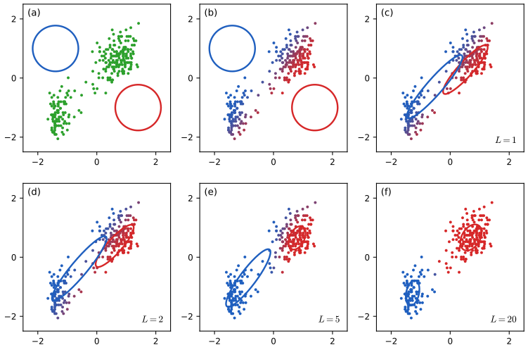
pp. 473–474 EM needs many more iterations than K-means, and each costs more, so K-means is a common initialiser. The likelihood has many local maxima, and EM finds one of them, not necessarily the largest. Mixtures can approximate complicated densities well, but the number of components needed can be very large, especially in many dimensions (Figure 15.8).
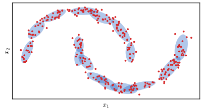
Filling the gap 15.3: how many components? p. 474, Figure 15.8
The book says the number of components "can become unacceptably large" in high dimensions. Here is a heuristic count, and an experiment that shows the other side of the trade-off.
Argument and experiment
A covering count (heuristic). Suppose the data lie near a smooth \(d\)-dimensional set of diameter \(\ell\) (a curve, \(d=1\), for the moons), and a component can represent the density well only over a region of radius about \(h\), within which the set looks flat and the density nearly constant. Covering the set by such regions takes about \((\ell/h)^d\) of them. So at a fixed accuracy the number of components grows exponentially with the intrinsic dimension \(d\), and the parameters per component (a \(D\times D\) covariance) grow with the ambient dimension \(D\). This is the motivation, in Chapter 16 and beyond, for models whose latent variables are continuous and whose maps from latent to data space are flexible.
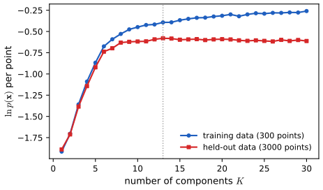
But more components also over-fit. Figure 15.S2 fits mixtures with \(K=1,\dots,30\) to 300 two-moons points (best of three starts) and scores them on 3000 new points. The training log likelihood keeps increasing (to \(-0.259\) per point at \(K=30\)); the held-out one rises steeply up to about \(K=8\), peaks at \(K=13\) (\(-0.580\)) and then slowly falls (\(-0.612\) at \(K=30\)). \(K\) is a model-complexity parameter and has to be chosen on held-out data or by a Bayesian criterion. ∎
15.3 Expectation–Maximization Algorithm
See also the companion course, Section 9.3 (an alternative view of EM) and Filling the gap 9.8.
pp. 474–477 Now let the latent variables take the lead. Collect them in \(\bZ\) (rows \(\bz_n^\T\)) and all parameters in \(\btheta\); for i.i.d. data the model is the plate diagram of Figure 15.9 (not reproduced). The log likelihood is
\[ \ln p(\bX\given\btheta)=\ln\Big\{\sum_\bZ p(\bX,\bZ\given\btheta)\Big\}. \tag{15.22} \]The sum over \(\bZ\) sits inside the logarithm. Even if \(p(\bX,\bZ\given\btheta)\) is in the exponential family (Section 3.4), \(p(\bX\given\btheta)\) usually is not: a mixture of two Gaussians is not Gaussian. For continuous \(\bZ\) the sum becomes an integral.
Definition 15.3 (complete data and the \(Q\) function) pp. 476–477, (15.23)–(15.24)
\(\{\bX,\bZ\}\) is the complete data set and \(\bX\) the incomplete one (Figure 15.5(a) and (b)). Maximising the complete-data log likelihood \(\ln p(\bX,\bZ\given\btheta)\) is assumed easy. Since \(\bZ\) is unknown, EM uses its posterior at the current parameters and the expected complete-data log likelihood
\[ Q(\btheta,\btheta^\old)=\sum_\bZ p(\bZ\given\bX,\btheta^\old)\ln p(\bX,\bZ\given\btheta). \tag{15.23} \]The M step is
\[ \btheta^\new=\argmax_\btheta Q(\btheta,\btheta^\old). \tag{15.24} \]Algorithm 15.3 (the general EM algorithm) p. 477
- Choose \(\btheta^\old\).
- E step: form \(Q(\btheta,\btheta^\old)\) from the posterior \(p(\bZ\given\bX,\btheta^\old)\) (in practice: compute the expected sufficient statistics it needs).
- M step: \(\btheta^\new=\argmax_\btheta Q(\btheta,\btheta^\old)\).
- Evaluate \(\ln p(\bX\given\btheta^\new)\) (the book's line "\(\mathcal L\gets p(\bX\given\btheta^\new)\)" is labelled "log likelihood" and should read \(\ln p\)); set \(\btheta^\old\gets\btheta^\new\) and repeat until convergence.
Each cycle increases \(\ln p(\bX\given\btheta)\) unless it is already at a stationary point (Result 15.11). With a prior \(p(\btheta)\), the M step maximises \(Q(\btheta,\btheta^\old)+\ln p(\btheta)\) instead (Exercise 15.5, Result 15.15), and suitable priors remove the singularities of Figure 15.6.
Filling the gap 15.4: missing values, and when they may be ignored p. 477
The book says EM handles missing data correctly when the values are "missing at random". The precise statement is short.
Derivation (short; the companion's Filling the gap 9.10 has more detail)
Split the data into observed and missing parts, \(\bx=(\bx_o,\bx_m)\), and let \(\mathbf m\) be the indicator of which entries are missing, with mechanism \(p(\mathbf m\given\bx,\bphi)\). What is actually observed is \((\bx_o,\mathbf m)\), with likelihood
\[ p(\bx_o,\mathbf m\given\btheta,\bphi)=\int p(\bx_o,\bx_m\given\btheta)\,p(\mathbf m\given\bx_o,\bx_m,\bphi)\,\d\bx_m . \]
If the mechanism depends only on what is observed, \(p(\mathbf m\given\bx_o,\bx_m,\bphi)=p(\mathbf m\given\bx_o,\bphi)\) (missing at random), the factor leaves the integral: \(p(\bx_o,\mathbf m\given\btheta,\bphi)\)
15.3.1 Gaussian mixtures
See also the companion course, Section 9.3.1 (Gaussian mixtures revisited) and Result 9.8.
pp. 478–479 With the labels observed (Figure 15.10), (15.9) and (15.10) give the complete-data likelihood
\[ p(\bX,\bZ\given\bmu,\Sig,\bpi)=\prod_{n=1}^N\prod_{k=1}^K\pi_k^{z_{nk}}\N(\bx_n\given\bmu_k,\Sig_k)^{z_{nk}} \tag{15.25} \] \[ \ln p(\bX,\bZ\given\bmu,\Sig,\bpi)=\sum_{n=1}^N\sum_{k=1}^Kz_{nk}\{\ln\pi_k+\ln\N(\bx_n\given\bmu_k,\Sig_k)\}. \tag{15.26} \]The sum and the logarithm have changed places: the log now acts on each Gaussian directly.
Result 15.6 (complete-data maximisation and the E and M steps) pp. 478–479, (15.26)–(15.30); Exercises 15.6, 15.8–15.10
- With \(\bZ\) known, (15.26) is maximised by fitting each component's mean and covariance to its own group of points, and by \[ \pi_k=\frac1N\sum_{n=1}^Nz_{nk}. \tag{15.27} \]
- The posterior over \(\bZ\) factorises over data points, \[ p(\bZ\given\bX,\bmu,\Sig,\bpi)\propto\prod_{n=1}^N\prod_{k=1}^K[\pi_k\N(\bx_n\given\bmu_k,\Sig_k)]^{z_{nk}} , \tag{15.28} \] and the expected indicator is the responsibility: \[ \E[z_{nk}]=\frac{\sum_{\bz_n}z_{nk}\prod_{k'}[\pi_{k'}\N(\bx_n\given\bmu_{k'},\Sig_{k'})]^{z_{nk'}}}{\sum_{\bz_n}\prod_j[\pi_j\N(\bx_n\given\bmu_j,\Sig_j)]^{z_{nj}}}=\frac{\pi_k\N(\bx_n\given\bmu_k,\Sig_k)}{\sum_{j=1}^K\pi_j\N(\bx_n\given\bmu_j,\Sig_j)}=\gamma(z_{nk}). \tag{15.29} \]
- Hence, by linearity, \[ \E_\bZ[\ln p(\bX,\bZ\given\bmu,\Sig,\bpi)]=\sum_{n=1}^N\sum_{k=1}^K\gamma(z_{nk})\{\ln\pi_k+\ln\N(\bx_n\given\bmu_k,\Sig_k)\}, \tag{15.30} \] and its maximum over the parameters, with the responsibilities fixed, is given exactly by (15.16), (15.18) and (15.21).
Proof (short; full derivations in the companion's Result 9.7 and Result 9.8)
(1) Grouping by \(k\), (15.26) is \(\sum_kN_k^{\mathrm c}\ln\pi_k\)
(2) (15.28) is (15.25) divided by \(p(\bX)\), a product of one factor per \(n\); so the \(\bz_n\) are independent given \(\bX\). (Graphically: every path between \(\bz_n\) and \(\bz_m\) in Figure 15.9 passes through a parameter node, which is fixed, so they are d-separated; Section 11.2.3.) In (15.29), \(\bz_n\) ranges over unit vectors and only \(\bz_n=\mathbf e_k\) contributes to the numerator.
(3) (15.30) has the same form as (15.26) with \(z_{nk}\) replaced by the weights \(\gamma(z_{nk})\), so the maximiser is the weighted version of (1): weighted means, weighted covariances, \(\pi_k=N_k/N\). The weighted log likelihood of a Gaussian is strictly concave in \((\Sig_k^{-1}\bmu_k,\Sig_k^{-1})\) when \(N_k>0\) and the weighted scatter is non-singular, so this stationary point is the unique maximum. ∎
Checks: enumerating all \(3^4\) joint labellings of 4 points reproduces the product of per-point posteriors to \(10^{-16}\); 300 random perturbations of the M-step solution all lower (15.30).
p. 480 For sequences, the labels can be linked in a Markov chain, giving the hidden Markov model of Figure 15.11; its E step passes messages along the chain (the forward–backward algorithm; companion course Section 13.2).
15.3.2 Relation to K-means
See also the companion course, Section 9.3.2 and Result 9.9.
pp. 480–481 Give every component the covariance \(\epsilon\bI\), with \(\epsilon\) a fixed constant:
\[ p(\bx\given\bmu_k,\Sig_k)=\frac1{(2\pi\epsilon)^{D/2}}\exp\Big\{-\frac1{2\epsilon}\|\bx-\bmu_k\|^2\Big\}. \tag{15.31} \]The responsibilities become
\[ \gamma(z_{nk})=\frac{\pi_k\exp\{-\|\bx_n-\bmu_k\|^2/2\epsilon\}}{\sum_j\pi_j\exp\{-\|\bx_n-\bmu_j\|^2/2\epsilon\}}. \tag{15.32} \]Result 15.7 (K-means is the small-variance limit of EM, with rates) pp. 480–481, (15.31)–(15.33); Exercise 15.12
Fix the means and weights with all \(\pi_k>0\). For a point \(\bx_n\) let \(d_{k}=\|\bx_n-\bmu_k\|^2\), let \(l\) be the unique nearest centre and \(\Delta_n=\min_{j\ne l}(d_j-d_l)>0\). Then
- \(\displaystyle 0\le1-\gamma(z_{nl})\le\frac{1-\pi_l}{\pi_l}\,e^{-\Delta_n/2\epsilon}\), so \(\gamma(z_{nk})\to r_{nk}\) exponentially fast, whatever the \(\pi_k\). At a tie (\(\Delta_n=0\)) the responsibilities do not harden: they converge to \(\pi\) restricted to the tied components and renormalised.
- The M step for the means, (15.16), tends to the K-means update (15.4) for every non-empty cluster.
- The expected complete-data log likelihood (15.30) diverges as \(\epsilon\to0\), but \[ \epsilon\,\E_\bZ[\ln p(\bX,\bZ\given\bmu,\Sig,\bpi)]\;\to\;-\frac12\sum_{n=1}^N\sum_{k=1}^Kr_{nk}\|\bx_n-\bmu_k\|^2=-\frac J2 . \] The book's version, \[ \E_\bZ[\ln p(\bX,\bZ\given\bmu,\Sig,\bpi)]\to-\frac12\sum_{n=1}^N\sum_{k=1}^Kr_{nk}\|\bx_n-\bmu_k\|^2+\const , \tag{15.33} \] should be read with this factor \(\epsilon\) (the "constant" there contains \(-\frac{ND}2\ln(2\pi\epsilon)\), which diverges, and the \(J\) term carries \(1/\epsilon\)). Either way, for each fixed \(\epsilon\) the \(\bmu\)-dependence of \(Q\) is \(-\frac1{2\epsilon}\sum_{n,k}\gamma(z_{nk})\|\bx_n-\bmu_k\|^2\), and in the limit maximising \(Q\) over the means is minimising \(J\).
Proof
(1) Divide numerator and denominator of (15.32) by \(e^{-d_l/2\epsilon}\): for \(k\ne l\), \[ \gamma(z_{nk})=\frac{\pi_ke^{-(d_k-d_l)/2\epsilon}}{\pi_l+\sum_{j\ne l}\pi_je^{-(d_j-d_l)/2\epsilon}}\le\frac{\pi_k}{\pi_l}e^{-\Delta_n/2\epsilon}, \] because the denominator is at least \(\pi_l\) and \(d_k-d_l\ge\Delta_n\). Summing over \(k\ne l\), \(1-\gamma(z_{nl})\le\frac{1-\pi_l}{\pi_l}e^{-\Delta_n/2\epsilon}\). If several centres tie at the minimum distance, their exponentials are equal and the others vanish, so \(\gamma\) tends to \(\pi_k/\sum_{j\,\text{tied}}\pi_j\) on the tied set: a hard limit needs a tie-breaking rule, as in Algorithm 15.1.
(2) \(\sum_n\gamma(z_{nk})\bx_n\to\sum_nr_{nk}\bx_n\) and \(\sum_n\gamma(z_{nk})\to\sum_nr_{nk}\), finite sums of convergent terms; the quotient converges when the limit denominator is positive.
(3) Insert \(\ln\N=-\frac D2\ln(2\pi\epsilon)-d_{nk}/2\epsilon\) in (15.30) and multiply by \(\epsilon\):
\[ \epsilon Q=\epsilon\sum_{n,k}\gamma(z_{nk})\ln\pi_k-\frac{ND}2\,\epsilon\ln(2\pi\epsilon)-\frac12\sum_{n,k}\gamma(z_{nk})d_{nk}. \]
The first term is bounded by \(\epsilon N\max_k|\ln\pi_k|\to0\); the second tends to 0 because \(\epsilon\ln\epsilon\to0\); and \(\big|\sum_{n,k}(\gamma(z_{nk})-r_{nk})d_{nk}\big|\)
Checks on Old Faithful at the K-means solution: the bound of (1) holds for every point at \(\epsilon=0.3,\dots,0.01\); \(|\epsilon Q+J/2|=5.6\), 0.18 and 0.003 at \(\epsilon=10^{-2},10^{-4},10^{-6}\) (\(J=79.58\)); EM with \(\epsilon=10^{-3}\) ends at the K-means centres to \(2\times10^{-16}\).
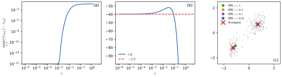
In the limit the weights \(\pi_k\) still get re-estimated as cluster fractions but no longer affect the assignments, and K-means does not estimate covariances at all.
15.3.3 Mixtures of Bernoulli distributions
See also the companion course, Section 9.3.3 (mixtures of Bernoulli distributions), and Section 3.1.1 of these notes (the Bernoulli distribution).
pp. 481–482 Mixtures of discrete distributions are also called latent class analysis (Lazarsfeld and Henry, 1968). For \(D\) binary variables with independent Bernoulli distributions,
\[ p(\bx\given\bmu)=\prod_{i=1}^D\mu_i^{x_i}(1-\mu_i)^{(1-x_i)} , \tag{15.34} \] \[ \E[\bx]=\bmu \tag{15.35} \] \[ \cov[\bx]=\diag\{\mu_i(1-\mu_i)\}. \tag{15.36} \]The mixture
\[ p(\bx\given\bmu,\bpi)=\sum_{k=1}^K\pi_kp(\bx\given\bmu_k) \tag{15.37} \] \[ p(\bx\given\bmu_k)=\prod_{i=1}^D\mu_{ki}^{x_i}(1-\mu_{ki})^{(1-x_i)} \tag{15.38} \]has
\[ \E[\bx]=\sum_{k=1}^K\pi_k\bmu_k \tag{15.39} \] \[ \cov[\bx]=\sum_{k=1}^K\pi_k\{\Sig_k+\bmu_k\bmu_k^\T\}-\E[\bx]\E[\bx]^\T , \tag{15.40} \]with \(\Sig_k=\diag\{\mu_{ki}(1-\mu_{ki})\}\).
Result 15.8 (moments of a Bernoulli vector and of any mixture) pp. 481–482; Exercises 15.13, 15.14
(15.35)–(15.36) hold, and for any mixture whose components have means \(\bmu_k\) and covariances \(\Sig_k\) (discrete, continuous or mixed), (15.39)–(15.40) hold. In particular a mixture of independent-bit distributions has non-zero covariances between bits, \(\cov[x_i,x_j]=\sum_k\pi_k\mu_{ki}\mu_{kj}-\bar\mu_i\bar\mu_j\) for \(i\ne j\): the latent label is what correlates them.
Proof (short; companion Result 9.10)
For one bit, \(\E[x_i]=0\cdot(1-\mu_i)+1\cdot\mu_i\) and \(\E[x_i^2]=\mu_i\), so \(\var[x_i]=\mu_i-\mu_i^2\); different bits are independent, so their covariance is 0. For a mixture, by the law of total expectation \(\E[\bx]=\sum_k\pi_k\E[\bx\given k]=\sum_k\pi_k\bmu_k\) and \(\E[\bx\bx^\T]=\sum_k\pi_k(\Sig_k+\bmu_k\bmu_k^\T)\); subtract \(\E[\bx]\E[\bx]^\T\). (Checked by enumerating all \(2^3\) states of a 3-bit mixture; \(\cov[x_1,x_2]=-0.112\) there.) ∎
pp. 482–483 The log likelihood
\[ \ln p(\bX\given\bmu,\bpi)=\sum_{n=1}^N\ln\Big\{\sum_{k=1}^K\pi_kp(\bx_n\given\bmu_k)\Big\} \tag{15.41} \]again has a sum inside the log. With a 1-of-K latent \(\bz\),
\[ p(\bx\given\bz,\bmu)=\prod_{k=1}^Kp(\bx\given\bmu_k)^{z_k} \tag{15.42} \] \[ p(\bz\given\bpi)=\prod_{k=1}^K\pi_k^{z_k} , \tag{15.43} \]whose product, summed over \(\bz\), is (15.37) (Exercise 15.16). The complete-data log likelihood and its expectation are
\[ \ln p(\bX,\bZ\given\bmu,\bpi)=\sum_{n=1}^N\sum_{k=1}^Kz_{nk}\Big\{\ln\pi_k+\sum_{i=1}^D[x_{ni}\ln\mu_{ki}+(1-x_{ni})\ln(1-\mu_{ki})]\Big\} \tag{15.44} \] \[ \E_\bZ[\ln p(\bX,\bZ\given\bmu,\bpi)]=\sum_{n=1}^N\sum_{k=1}^K\gamma(z_{nk})\Big\{\ln\pi_k+\sum_{i=1}^D[x_{ni}\ln\mu_{ki}+(1-x_{ni})\ln(1-\mu_{ki})]\Big\} \tag{15.45} \]with E step
\[ \gamma(z_{nk})=\E[z_{nk}]=\frac{\sum_{\bz_n}z_{nk}\prod_{k'}[\pi_{k'}p(\bx_n\given\bmu_{k'})]^{z_{nk'}}}{\sum_{\bz_n}\prod_j[\pi_jp(\bx_n\given\bmu_j)]^{z_{nj}}}=\frac{\pi_kp(\bx_n\given\bmu_k)}{\sum_{j=1}^K\pi_jp(\bx_n\given\bmu_j)} . \tag{15.46} \]The responsibilities enter (15.45) only through
\[ N_k=\sum_{n=1}^N\gamma(z_{nk}) \tag{15.47} \] \[ \bar\bx_k=\frac1{N_k}\sum_{n=1}^N\gamma(z_{nk})\bx_n , \tag{15.48} \]and the M step is
\[ \bmu_k=\bar\bx_k \tag{15.49} \] \[ \pi_k=\frac{N_k}N . \tag{15.50} \]Result 15.9 (EM for Bernoulli mixtures) pp. 482–484; Exercises 15.15–15.19
- (15.49)–(15.50) maximise (15.45) for fixed responsibilities.
- The likelihood is bounded: \(\ln p(\bX\given\bmu,\bpi)\le0\). There are no singularities with \(\ln p\to+\infty\). It can be 0 (log \(-\infty\)) only if some \(\bx_n\) has probability 0 under every component, which EM never reaches from a start with all \(\mu_{ki}\in(0,1)\), since it never decreases the likelihood.
- After every M step, \(\sum_k\pi_k\bmu_k=\frac1N\sum_n\bx_n=\bar\bx\) exactly; in particular at a maximum \(\E[\bx]=\bar\bx\). If all components start equal, EM sets every \(\bmu_k=\bar\bx\) after one iteration and stays there: a degenerate fixed point.
Proof (short; companion Result 9.11 and Exercises 9.13–9.17)
(1) \(\partial/\partial\mu_{ki}\) of (15.45) is \(\sum_n\gamma(z_{nk})\big(\frac{x_{ni}}{\mu_{ki}}-\frac{1-x_{ni}}{1-\mu_{ki}}\big)\)
(2) Each \(p(\bx_n\given\bmu_k)\) is a probability of a discrete outcome, at most 1, so each mixture term is at most \(\sum_k\pi_k=1\) and each log term at most 0.
(3) \(\sum_k\pi_k\bmu_k\)
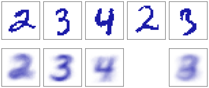
p. 484 Handwritten digits. Figure 15.12 binarises MNIST digits at 0.5 and fits \(K=3\) components by 10 EM iterations to 600 images of the digits 2, 3 and 4, with \(\pi_k=1/K\) and the \(\mu_{ki}\) drawn uniformly in \((0.25,0.75)\).
Filling the gap 15.5: the book's starting values, and local maxima p. 484
The book adds that the random \(\mu_{kj}\) were "normalized to satisfy the constraint that \(\sum_j\mu_{kj}=1\)". There is no such constraint for Bernoulli parameters.
Explanation and experiment
Each \(\mu_{ki}\) is the probability that pixel \(i\) is on in component \(k\); the 784 probabilities of one component are unrelated and need not sum to anything. A constraint \(\sum_j\mu_{kij}=1\) belongs to the multinomial model of Exercise 15.20, where it runs over the states of one variable. Normalising is harmless, though: it only changes the start. Every \(\mu_{ki}\) becomes about \(1/784\), so every image is very unlikely under every component (\(\ln p(\bX)=-434{,}819\) at the start), but the E step only uses differences of log likelihoods between components. These are random, of a few nats, so the first responsibilities are a nearly hard random split of the images, and the first M step replaces each \(\bmu_k\) by the mean image of its share (\(\ln p\) jumps to \(-118{,}368\)). From there EM proceeds normally: after 10 iterations \(\ln p=-111{,}380.7\), the three means look like a 2, a 3 and a 4, and 517 of the 600 images are in their own digit's component.
Local maxima. Over twelve seeds of the generator, the same recipe gives three components with different majority digits in 9 runs, but only 4 runs put more than 490 of the 600 images with their own digit; in the others two components share a digit or split the 2s and 3s between them (preset 2 of the demo, from a uniform start: \(\ln p/N=-185.99\) after 30 iterations, against \(-185.42\) when the start of Figure 15.12 is run for 30 iterations). The best log likelihood does not always come with the best agreement with the labels: clusters are not classes. ∎
The extension to variables with \(M>2\) states uses the discrete distribution (3.14); it is Exercise 15.20.
15.4 Evidence Lower Bound
See also the companion course, Section 9.4 (the EM algorithm in general), Section 10.1 (variational inference) and the EM bound demo; Section 2.5.5 of these notes (the Kullback–Leibler divergence).
pp. 485–486 The third and most general view of EM rests on a lower bound on the log likelihood, the evidence lower bound (ELBO), also called the variational lower bound. "Evidence" is the (marginal) likelihood, the quantity that compares models in a Bayesian setting. Let \(\bX\) be all observed and \(\bZ\) all latent variables, with joint \(p(\bX,\bZ\given\btheta)\). The goal is to maximise
\[ p(\bX\given\btheta)=\sum_\bZ p(\bX,\bZ\given\btheta) , \tag{15.51} \]assuming the complete-data likelihood is much easier to handle. (For continuous or mixed \(\bZ\) replace sums by integrals.)
Definition 15.4 (the evidence lower bound and the gap) p. 485, (15.53)–(15.54)
For a distribution \(q(\bZ)\) over the latent variables,
\[ \LB(q,\btheta)=\sum_\bZ q(\bZ)\ln\Big\{\frac{p(\bX,\bZ\given\btheta)}{q(\bZ)}\Big\} \tag{15.53} \] \[ \KL(q\|p)=-\sum_\bZ q(\bZ)\ln\Big\{\frac{p(\bZ\given\bX,\btheta)}{q(\bZ)}\Big\} . \tag{15.54} \]\(\LB\) is a functional of \(q\) and a function of \(\btheta\); it contains the joint \(p(\bX,\bZ)\), while the KL term contains the posterior \(p(\bZ\given\bX)\), and the signs differ. Terms with \(q(\bZ)=0\) are 0 (\(0\ln0=0\)).
Result 15.10 (the decomposition and the bound) pp. 485–486, (15.52), (15.55), Figure 15.13; Exercise 15.21
For every distribution \(q(\bZ)\) and every \(\btheta\) with \(p(\bX\given\btheta)>0\),
\[ \ln p(\bX\given\btheta)=\LB(q,\btheta)+\KL(q\|p) , \tag{15.52} \]and \(\KL(q\|p)\ge0\) with equality if and only if \(q(\bZ)=p(\bZ\given\bX,\btheta)\). Hence \(\LB(q,\btheta)\le\ln p(\bX\given\btheta)\), with equality exactly at the posterior.
Proof
The identity. By the product rule,
\[ \ln p(\bX,\bZ\given\btheta)=\ln p(\bZ\given\bX,\btheta)+\ln p(\bX\given\btheta) \tag{15.55} \]for every \(\bZ\) with \(p(\bX,\bZ\given\btheta)>0\). Suppose first that \(q(\bZ)>0\) only where \(p(\bZ\given\bX,\btheta)>0\). For such \(\bZ\), subtract \(\ln q(\bZ)\) from both sides of (15.55), multiply by \(q(\bZ)\) and sum: \[ \sum_\bZ q\ln\frac{p(\bX,\bZ\given\btheta)}q=\sum_\bZ q\ln\frac{p(\bZ\given\bX,\btheta)}q+\ln p(\bX\given\btheta)\sum_\bZ q , \] that is \(\LB=-\KL+\ln p(\bX\given\btheta)\), using \(\sum_\bZ q(\bZ)=1\). If instead \(q\) puts mass on some \(\bZ\) with \(p(\bZ\given\bX,\btheta)=0\), then \(\LB=-\infty\) and \(\KL=+\infty\), and (15.52) holds in the extended sense. For continuous \(\bZ\) the same computation works with integrals, whenever \(\int q\ln q\) is finite.
Non-negativity. \(\ln\) is strictly concave, so by Jensen's inequality, with the sum over the support of \(q\), \[ -\KL(q\|p)=\sum_\bZ q\ln\frac{p(\bZ\given\bX)}{q}\le\ln\sum_\bZ q\frac{p(\bZ\given\bX)}{q}=\ln\sum_{\bZ:\,q>0}p(\bZ\given\bX)\le\ln1=0 . \] Equality in the first step needs \(p/q\) constant on the support of \(q\), and in the second that the support carries all posterior mass; together, \(q=p(\cdot\given\bX,\btheta)\). (This is Section 2.5.5 of the book; the margin note on p. 486 points to Section 2.5.7, which is mutual information.) ∎
A one-line route to the bound. Directly, \(\ln p(\bX)=\ln\sum_\bZ q\,\frac{p(\bX,\bZ)}q\)
Filling the gap 15.6: the ELBO in the form used by variational autoencoders and diffusion models p. 485; used in Chapters 19 and 20
The book introduces the ELBO here because later chapters maximise it with neural networks. We rewrite it in the per-example form those chapters use and say what changes when \(q\) can no longer be the exact posterior.
Derivation
Per-example form. For i.i.d. data, \(p(\bX,\bZ\given\btheta)=\prod_np(\bx_n\given\bz_n,\btheta)p(\bz_n\given\btheta)\). Take a factorised \(q(\bZ)=\prod_nq_n(\bz_n)\) (no loss for the exact E step, because the posterior itself factorises, (15.57)). Then the log of the ratio in (15.53) is a sum over \(n\), each term depends only on \(\bz_n\), and the expectation of each term under \(q\) is an expectation under \(q_n\) alone:
\[ \LB(q,\btheta)=\sum_{n=1}^N\Big\{\underbrace{\E_{q_n(\bz_n)}[\ln p(\bx_n\given\bz_n,\btheta)]}_{\text{reconstruction}}-\underbrace{\KL\big(q_n(\bz_n)\,\|\,p(\bz_n\given\btheta)\big)}_{\text{regulariser}}\Big\}. \]
The first term rewards latent values that explain \(\bx_n\); the second keeps \(q_n\) close to the prior. For the Gaussian mixture, \(q_n\) is a vector of \(K\) probabilities \(q_{nk}\) and this reads \(\sum_n\sum_kq_{nk}\ln\N(\bx_n\given\bmu_k,\Sig_k)\)
Amortised and restricted \(q\). In a variational autoencoder (Chapter 19 of the book) \(\bz\) is continuous, the exact posterior is intractable, and \(q_n(\bz)=q(\bz\given\bx_n,\bphi)\) is produced by a network (the encoder) with parameters \(\bphi\) shared by all data points. EM's exact E step is replaced by gradient steps on \(\bphi\), its M step by gradient steps on \(\btheta\), both on the same objective \(\LB(\bphi,\btheta)\). By (15.52), \(\sum_n\ln p(\bx_n\given\btheta)-\LB\)
The gradient of the bound in \(\btheta\). Since \(q\) does not depend on \(\btheta\), \(\nabla_\btheta\LB(q,\btheta)=\E_q[\nabla_\btheta\ln p(\bX,\bZ\given\btheta)]\); at \(q\) equal to the posterior this is exactly \(\nabla_\btheta\ln p(\bX\given\btheta)\) (Result 15.12). This is why a stochastic estimate of the ELBO gradient is a useful substitute for the intractable likelihood gradient. ∎
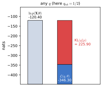
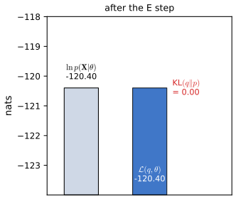
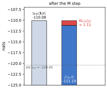
Figures 15.13–15.15 use the 60 points of the demo's "two clusters" data, a two-component 1-D mixture and the start \(\bpi=(0.3,0.7)\), \(\bmu=(-2.5,0.5)\), \(\sigma^2=(0.5,3)\): the first three half steps of preset 1 of the demo.
15.4.1 EM revisited
See also the companion course, Result 9.15 (EM never decreases the log likelihood) and Result 9.16 (tangency).
pp. 486–488 (15.52) turns EM into a two-variable optimisation of \(\LB(q,\btheta)\).
Result 15.11 (EM is coordinate ascent on the ELBO, and each cycle gains at least as much as the bound) pp. 486–487, (15.56), Figures 15.14–15.15
- E step: \(\argmax_q\LB(q,\btheta^\old)=p(\bZ\given\bX,\btheta^\old)\), and there \(\LB=\ln p(\bX\given\btheta^\old)\).
- M step: with \(q^\old=p(\bZ\given\bX,\btheta^\old)\), \[ \LB(q^\old,\btheta)=\sum_\bZ p(\bZ\given\bX,\btheta^\old)\ln p(\bX,\bZ\given\btheta)-\sum_\bZ p(\bZ\given\bX,\btheta^\old)\ln p(\bZ\given\bX,\btheta^\old)=Q(\btheta,\btheta^\old)+\const , \tag{15.56} \] the constant being the entropy of \(q^\old\); so maximising \(\LB(q^\old,\cdot)\) is (15.24).
- The gain. Exactly, \[ \ln p(\bX\given\btheta^\new)-\ln p(\bX\given\btheta^\old)=\underbrace{Q(\btheta^\new,\btheta^\old)-Q(\btheta^\old,\btheta^\old)}_{\ge0}+\underbrace{\KL\big(q^\old\,\|\,p(\cdot\given\bX,\btheta^\new)\big)}_{\ge0}, \] so the log likelihood increases at least as much as the bound, and it stays constant only if \(\btheta^\old\) already maximises \(Q(\cdot,\btheta^\old)\) and the posterior does not change.
Proof
(1) \(\ln p(\bX\given\btheta^\old)\) does not depend on \(q\), so by (15.52) maximising \(\LB\) over \(q\) means minimising \(\KL(q\|p)\ge0\), which is 0 only at the posterior (Result 15.10).
(2) Substitute \(q^\old\) into (15.53) and split the logarithm of the ratio.
(3) Apply (15.52) at \(\btheta^\new\) and at \(\btheta^\old\) with the same \(q^\old\): \(\ln p(\bX\given\btheta^\new)=\LB(q^\old,\btheta^\new)\)
What monotonicity does and does not give. The values \(\ln p(\bX\given\btheta^{(t)})\) increase; if the likelihood is bounded above (it is not for unregularised Gaussian mixtures, Result 15.3) they converge. That the parameters converge, and to a stationary point, needs extra conditions (Wu, 1983): for instance continuity of \(Q\) in both arguments and isolated stationary points. In the demo's preset 1 the first M step raises \(\LB\) by 9.203 and \(\ln p\) by 10.312, the difference being the new KL 1.109 (checked to \(10^{-10}\)).
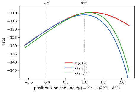
Result 15.12 (the bound touches the log likelihood: equal value, equal slope, at least as much curvature) pp. 487–488, Figure 15.16; Exercise 15.22
Let \(q^\old=p(\bZ\given\bX,\btheta^\old)\) and assume \(p(\bX,\bZ\given\btheta)\) is twice differentiable in \(\btheta\). Then \(\ln p(\bX\given\btheta)-\LB(q^\old,\btheta)\)
- \(\nabla_\btheta\LB(q^\old,\btheta)\big|_{\btheta^\old}=\nabla_\btheta\ln p(\bX\given\btheta)\big|_{\btheta^\old}\), and both equal \(\E_{q^\old}[\nabla_\btheta\ln p(\bX,\bZ\given\btheta)]\) at \(\btheta^\old\) (Fisher's identity);
- \(\nabla^2_\btheta\ln p(\bX\given\btheta)-\nabla^2_\btheta\LB(q^\old,\btheta)\succeq0\) at \(\btheta^\old\): the bound bends down at least as fast as the log likelihood.
Proof
The difference \(g(\btheta)=\ln p(\bX\given\btheta)-\LB(q^\old,\btheta)\) is the KL divergence (15.52), so \(g\ge0\) everywhere and \(g(\btheta^\old)=0\): \(\btheta^\old\) is a minimum of the smooth function \(g\), hence \(\nabla g=\bzero\) and \(\nabla^2g\succeq0\) there. For Fisher's identity directly: \(\nabla\ln p(\bX\given\btheta)\)
Checked by central differences in all six coordinates \((\mu_k,\ln\sigma_k^2,\ln\pi_k)\) of the demo's model: the gradients agree to \(4\times10^{-8}\) while their size is up to 16. A consequence: a fixed point of EM (\(\btheta^\new=\btheta^\old\)) is a stationary point of \(\ln p\), since there \(\nabla\ln p=\nabla\LB(q^\old,\cdot)=\bzero\).
p. 488 The book says the bound "is a convex function having a unique maximum (for mixture components from the exponential family)". A function with a unique maximum of this kind is concave, and even concavity depends on the coordinates.
Result 15.13 (the M-step objective is concave in the natural parameters; erratum for "convex") p. 488
Suppose the complete-data distribution is an exponential family in natural parameters \(\bEta\), \(p(\bX,\bZ\given\bEta)\)
- \(\LB(q,\bEta)=\bEta^\T\E_q[\bu]-A(\bEta)+\const\) is concave in \(\bEta\), strictly if the representation is minimal, and its maximiser (when it exists) is unique and solves the moment-matching equation \(\nabla A(\bEta)=\E_q[\bu]\);
- in other coordinates the maximiser is the same point, but the function need not be concave: for one Gaussian term in \((\mu,\sigma^2)\), \(f(\mu,\sigma^2)=-\frac12\ln\sigma^2-S/(2\sigma^2)\) (with \(\mu\) at the weighted mean and \(S\) the weighted mean square) has \(\partial^2f/\partial(\sigma^2)^2=\frac1{2\sigma^4}-\frac S{\sigma^6}>0\) whenever \(\sigma^2>2S\).
Proof
(1) \(\ln p(\bX,\bZ\given\bEta)=\ln h+\bEta^\T\bu-A(\bEta)\); taking \(\E_q\) and adding the entropy of \(q\) (which does not depend on \(\bEta\)) gives the form stated. \(A\) is convex: its Hessian is the covariance of \(\bu\) under the model, \(\nabla^2A=\cov_\bEta[\bu]\succeq0\) (Section 3.4), positive definite for a minimal representation. A linear function minus a (strictly) convex one is (strictly) concave; a strictly concave function has at most one maximiser, and setting the gradient to zero gives \(\nabla A(\bEta)=\E_q[\bu]\). For the Gaussian mixture the per-component natural parameters are \((\Sig_k^{-1}\bmu_k,-\frac12\Sig_k^{-1})\), and the categorical term \(\sum_kN_k\ln\pi_k\) is concave in the logits \(a_k\), since \(\ln\pi_k=a_k-\ln\sum_je^{a_j}\) and log-sum-exp is convex.
(2) Direct differentiation. Uniqueness of the maximiser is a property of the point, so it survives a change of coordinates; concavity is not. ∎
Checked: at 50 random points the Hessian in natural parameters of a weighted Gaussian term from the demo has largest eigenvalue \(-0.45\) or less; in \((\mu,\sigma^2)\) at \(\sigma^2=5S\) it has a positive eigenvalue (2.16).
The E and M steps both increase a well-defined bound, and each full cycle increases \(\ln p\) unless the parameters are already at a maximum, in which case they do not change.
15.4.2 Independent and identically distributed data
pp. 488–489 For i.i.d. data, \(p(\bX,\bZ)=\prod_np(\bx_n,\bz_n)\) and \(p(\bX)=\prod_np(\bx_n)\).
Result 15.14 (the posterior factorises over data points) p. 488, (15.57); Exercise 15.6
\[ p(\bZ\given\bX,\btheta)=\frac{p(\bX,\bZ\given\btheta)}{\sum_\bZ p(\bX,\bZ\given\btheta)}=\frac{\prod_{n=1}^Np(\bx_n,\bz_n\given\btheta)}{\sum_\bZ\prod_{n=1}^Np(\bx_n,\bz_n\given\btheta)}=\prod_{n=1}^Np(\bz_n\given\bx_n,\btheta) \tag{15.57} \]Proof
The sum over \(\bZ=(\bz_1,\dots,\bz_N)\) of a product of functions of single \(\bz_n\) is the product of the single sums: \(\sum_\bZ\prod_nf_n(\bz_n)=\prod_n\sum_{\bz_n}f_n(\bz_n)\) (distributivity). So the ratio is \(\prod_nf_n(\bz_n)/\sum_{\bz_n'}f_n(\bz_n')\)
15.4.3 Parameter priors
See also the companion course, Filling the gap 9.9 (the MAP version, and a prior that prevents collapse).
p. 489 As a function of \(\btheta\), \(p(\btheta\given\bX)=p(\btheta,\bX)/p(\bX)\), so
\[ \ln p(\btheta\given\bX)=\ln p(\btheta,\bX)-\ln p(\bX). \tag{15.58} \]Result 15.15 (EM for the posterior mode) p. 489, (15.58)–(15.59); Exercise 15.5
Using (15.52) for \(\ln p(\bX\given\btheta)\),
\[ \ln p(\btheta\given\bX)=\LB(q,\btheta)+\KL(q\|p)+\ln p(\btheta)-\ln p(\bX)\ \ge\ \LB(q,\btheta)+\ln p(\btheta)-\ln p(\bX) , \tag{15.59} \]with \(\ln p(\bX)\) constant. Alternating maximisation of the right side gives the same E step as before and the M step \(\btheta^\new=\argmax_\btheta\{Q(\btheta,\btheta^\old)\)
Proof
\(\ln p(\btheta,\bX)=\ln p(\bX\given\btheta)+\ln p(\btheta)\); substitute (15.52) and drop \(\KL\ge0\). \(q\) appears only in \(\LB\), so the E step is unchanged; with \(q=q^\old\), \(\LB(q^\old,\btheta)=Q(\btheta,\btheta^\old)+\const\) by (15.56). The monotonicity argument of Result 15.11 applies verbatim to \(F(\btheta)=\ln p(\bX\given\btheta)+\ln p(\btheta)\). ∎
Filling the gap 15.7: a prior that removes the singularities p. 489
The book says the prior term "has the effect of removing the singularities". Here is an explicit prior, its M step, and why the objective becomes bounded.
Derivation
Take a one-dimensional mixture and an inverse-gamma prior on each variance, \(p(\sigma_k^2)\propto(\sigma_k^2)^{-(a_0+1)}e^{-b_0/\sigma_k^2}\) with \(a_0,b_0>0\). The M-step objective for \(v=\sigma_k^2\) (with \(\mu_k\) at the weighted mean and \(S_k=\sum_n\gamma(z_{nk})(x_n-\mu_k)^2\)) is
\[ -\frac{N_k}2\ln v-\frac{S_k}{2v}-(a_0+1)\ln v-\frac{b_0}v , \]
whose derivative \(-\big(\frac{N_k}2+a_0+1\big)\frac1v+\big(\frac{S_k}2+b_0\big)\frac1{v^2}\) vanishes at
\[ \sigma_k^2=\frac{S_k+2b_0}{N_k+2(a_0+1)}\ \ge\ \frac{2b_0}{N+2a_0+2}>0 . \]
So no variance can reach 0. More strongly, the MAP objective is bounded above: each likelihood term satisfies \(\ln\{\sum_k\pi_k\N(x_n\given\mu_k,v_k)\}\)
The demo uses \(a_0=2\), \(b_0=0.1\). Started with a narrow component on the largest of the 60 points, maximum likelihood drives its variance to the \(10^{-10}\) floor within a few half steps; with the prior that variance rises from its starting value 0.010 to 0.029 at the first M step and stays there (the guaranteed lower bound is 0.0030), and \(\ln p(\bX\given\btheta)+\ln p(\btheta)\) never decreases (checked). The prior removes the singularity but not the poor local maximum: the component still sits on the outlying point. ∎
15.4.4 Generalized EM
See also the companion course, Result 9.18 (maxima of the bound are maxima of the likelihood).
pp. 489–490 When the M step cannot be done exactly, the generalised EM (GEM) algorithm only asks it to increase \(\LB(q,\btheta)\), for instance by a few gradient steps, or by maximising over groups of parameters in turn (expectation conditional maximisation, ECM; Meng and Rubin, 1993). Symmetrically, the E step can be partial (Neal and Hinton, 1999).
Result 15.16 (generalised steps keep the monotonicity; local maxima correspond) pp. 489–490
- If \(\LB(q^\old,\btheta^\new)\ge\LB(q^\old,\btheta^\old)\) with \(q^\old\) the posterior at \(\btheta^\old\), then \(\ln p(\bX\given\btheta^\new)\ge\ln p(\bX\given\btheta^\old)\).
- \(\LB(\cdot,\btheta)\) is concave in \(q\); in particular every partial E step \(q\gets(1-\lambda)q+\lambda\,p(\bZ\given\bX,\btheta)\), \(0<\lambda\le1\), does not decrease \(\LB\).
- If \((q^\star,\btheta^\star)\) is a local maximum of \(\LB\), then \(q^\star=p(\bZ\given\bX,\btheta^\star)\) and \(\btheta^\star\) is a local maximum of \(\ln p(\bX\given\btheta)\); conversely, a local maximum \(\btheta^\star\) of \(\ln p\) gives the local maximum \((p(\cdot\given\bX,\btheta^\star),\btheta^\star)\) of \(\LB\). The same holds for global maxima.
Proof
(1) \(\ln p(\bX\given\btheta^\new)\ge\LB(q^\old,\btheta^\new)\)
(2) \(\LB(q,\btheta)=\sum_\bZ q\ln p(\bX,\bZ\given\btheta)+H(q)\): linear in \(q\) plus the entropy, which is concave (\(-t\ln t\) is concave). Along the segment \(q_\lambda=(1-\lambda)q+\lambda q^\star\) to the maximiser \(q^\star\), concavity gives \(\LB(q_\lambda)\ge(1-\lambda)\LB(q)\)
(3) Write \(q_\btheta=p(\cdot\given\bX,\btheta)\). Assume \(p(\bX,\bZ\given\btheta)\) is continuous in \(\btheta\) and \(p(\bX\given\btheta)>0\), so \(\btheta\mapsto q_\btheta\) is continuous. (\(\Rightarrow\)) For fixed \(\btheta^\star\), \(\LB(\cdot,\btheta^\star)\) is strictly concave on the probability simplex (the entropy is strictly concave), so a local maximiser is the global one, \(q^\star=q_{\btheta^\star}\). For \(\btheta\) close enough to \(\btheta^\star\), \(q_\btheta\) is close to \(q^\star\), so \((q_\btheta,\btheta)\) lies in the neighbourhood where \(\LB\le\LB(q^\star,\btheta^\star)\), and \(\ln p(\bX\given\btheta)=\LB(q_\btheta,\btheta)\)
Checks: partial E steps with \(\lambda=0.3\) never decrease \(\LB\) and leave a gap (0.096 after the second E step); ECM never decreases \(\LB\) or \(\ln p\); a gradient M step of size \(\eta=1\) is a valid GEM step but \(\eta=4\) overshoots and \(\LB\) falls at half steps 10, 12, 14, ...; at the converged EM solution the gradient of \(\ln p\) is \(10^{-9}\) and its Hessian has no positive eigenvalue (one zero eigenvalue, because the logits are defined up to a constant).
15.4.5 Sequential EM
See also the companion course, Result 9.19 and Algorithm 9.6 (incremental EM).
p. 490 Because \(\LB\) separates over data points, \(\LB=\sum_n\LB_n(q_n,\btheta)\), one can recompute the responsibilities of a single point \(\bx_m\) and then update the parameters. For exponential-family components the M step needs only sufficient statistics, which change by a single term. For the means, with \(\gamma^\old(z_{mk})\) and \(\gamma^\new(z_{mk})\) the old and new responsibilities,
\[ \bmu_k^\new=\bmu_k^\old+\Big(\frac{\gamma^\new(z_{mk})-\gamma^\old(z_{mk})}{N_k^\new}\Big)(\bx_m-\bmu_k^\old) \tag{15.60} \] \[ N_k^\new=N_k^\old+\gamma^\new(z_{mk})-\gamma^\old(z_{mk}). \tag{15.61} \]Result 15.17 (incremental updates of the means, covariances and weights) p. 490, (15.60)–(15.61); Exercises 15.23, 15.24
Let \(d=\gamma^\new(z_{mk})-\gamma^\old(z_{mk})\), \(a=d/N_k^\new\) and \(\bdelta=\bx_m-\bmu_k^\old\). Then (15.60)–(15.61) hold, and
\[ \Sig_k^\new=\Sig_k^\old+a\big[(1-a)\bdelta\bdelta^\T-\Sig_k^\old\big],\qquad\pi_k^\new=\pi_k^\old+\frac dN . \]Each step (one exact partial E step for \(\bx_m\), then the exact M step) does not decrease \(\LB\), so the log likelihood behaves as in Result 15.16.
Proof
Means. \(N_k\bmu_k=\sum_n\gamma(z_{nk})\bx_n\) changes by \(d\,\bx_m\): \(N_k^\new\bmu_k^\new=N_k^\old\bmu_k^\old\)
Covariances. \(\sum_n\gamma(z_{nk})\bx_n\bx_n^\T=N_k(\Sig_k+\bmu_k\bmu_k^\T)\) changes by \(d\,\bx_m\bx_m^\T\), so \(\Sig_k^\new=\frac{N_k^\old}{N_k^\new}(\Sig_k^\old\)
Weights and monotonicity. \(\pi_k=N_k/N\) and \(N\) is unchanged. Replacing \(q_m\) by the posterior maximises the separable \(\LB\) over \(q_m\) with the other \(q_n\) fixed, and the M step maximises over \(\btheta\). ∎ (All three updates agree with recomputing (15.16), (15.18), (15.21) from scratch to \(10^{-12}\).)
Algorithm 15.4 (incremental EM for a Gaussian mixture; Neal and Hinton, 1999)
- Run one full E step and keep the statistics \(N_k\), \(\sum_n\gamma(z_{nk})\bx_n\), \(\sum_n\gamma(z_{nk})\bx_n\bx_n^\T\); compute the parameters from them.
- For each point \(m\) in turn (a random order per pass): recompute \(\gamma(z_{mk})\) with the current parameters, add the change times \(1\), \(\bx_m\), \(\bx_m\bx_m^\T\) to the statistics, recompute the parameters.
- Repeat passes until \(\ln p\) stops changing.
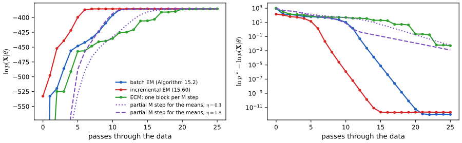
Both the E and the M step take a time independent of \(N\), and since the parameters are revised after each point the incremental version can converge faster than the batch one; if it converges to a local (or global) maximum of \(\LB\), that is a local (or global) maximum of \(\ln p(\bX\given\btheta)\) (Result 15.16).
Summary: errors and imprecisions found in the chapter (first printing)
- Algorithm 15.1 (p. 462): the loop "for \(N\in\{1,\dots,N\}\)" should run over \(n\). Algorithm 15.2 (p. 475) returns "\(\{\bx_k\}\)" for \(\{\bmu_k\}\). Algorithm 15.3 (p. 477): the line commented "Evaluate log likelihood" assigns \(p(\bX\given\btheta^\new)\), not \(\ln p\).
- (15.14) (p. 469): \((2\pi)^{-1/2}\sigma_j^{-1}\) is the case \(D=1\); for \(\Sig_j=\sigma_j^2\bI\) in \(D\) dimensions the value is \((2\pi)^{-D/2}\sigma_j^{-D}\) (checked; the conclusion is unchanged).
- (15.33) (p. 481): as written the left side diverges; the precise statement is \(\epsilon\,\E_\bZ[\ln p]\to-J/2\) (Result 15.7; checked to \(3\times10^{-3}\) at \(\epsilon=10^{-6}\)).
- p. 484: Bernoulli parameters are not subject to \(\sum_j\mu_{kj}=1\); normalising the random start is harmless but not a constraint (Filling the gap 15.5).
- p. 486, margin: the non-negativity of the KL divergence is shown in Section 2.5.5 (Section 2.5.7 is mutual information). p. 487: the sentence "as we saw earlier distribution for mixtures of Gaussians" is garbled; read "as we saw earlier for mixtures of Gaussians".
- p. 488: "This bound is a convex function having a unique maximum" should be concave, and concavity holds in the natural parameters, not in all coordinates; in \((\mu,\sigma^2)\) it fails for \(\sigma^2>2S\) (Result 15.13; checked).
- Margins on pp. 472 and 484 point to Section 15.3 for the proof that EM increases the likelihood; the proof is in Section 15.4.1.
- Figure 15.8: the axis labels appear exchanged (\(x_1\) on the vertical axis, \(x_2\) on the horizontal one).
- p. 470 (imprecision): there are \(K!\) equivalent parameter vectors only when the components are distinct (Result 15.4). p. 461 (imprecision): finite termination of K-means needs a tie-breaking rule (Result 15.1).
Exercises
All 24 exercises of Chapter 15 (Bishop and Bishop, 2024, pp. 490–493), restated in my own words, with complete solutions (hidden). Stars give the book's difficulty. The official solutions manual stops at Chapter 10, so these solutions are my own; where a companion-course exercise is the same, it is linked.
Exercise 15.1 (★). Using that there are finitely many assignments \(\{r_{nk}\}\), and that each has a unique optimal set of prototypes, show that K-means converges after finitely many iterations.
Solution
Let \(\mathbf r^{(t)}\) be the assignment after the \(t\)th E step and \(\bmu^{(t)}=\bmu(\mathbf r^{(t)})\) the M-step prototypes (cluster means; an empty cluster keeps its old prototype). Both steps are exact minimisations (Result 15.1), so \(J(\mathbf r^{(t+1)},\bmu^{(t+1)})\le J(\mathbf r^{(t+1)},\bmu^{(t)})\)
\({}\le J(\mathbf r^{(t)},\bmu^{(t)})\). With the rule "change a label only if another centre is strictly closer", either \(\mathbf r^{(t+1)}=\mathbf r^{(t)}\) (the algorithm stops) or some point moved strictly closer and the second inequality is strict. So, as long as the algorithm runs, the values \(J(\mathbf r^{(t)},\bmu(\mathbf r^{(t)}))\) strictly decrease, no assignment can occur twice, and since there are at most \(K^N\) assignments it stops after at most \(K^N\) iterations. (With a different deterministic tie rule the same conclusion holds: if \(J\) does not strictly decrease then \(\bmu^{(t+1)}=\bmu^{(t)}\) by uniqueness of the M step, and the next E step reproduces \(\mathbf r^{(t+1)}\).) Companion Exercise 9.1. Exercise 15.2 (★★). Derive the sequential K-means update (15.5) from the batch formula (15.4) by separating the contribution of the last point assigned, and note that each prototype remains the mean of the points assigned to it.
Solution
See Filling the gap 15.1: with \(m\) points in the cluster, \(\bmu^{(m)}=\frac{m-1}m\bmu^{(m-1)}\)
\({}+\frac1m\bx_{(m)}=\bmu^{(m-1)}+\frac1m(\bx_{(m)}\) \({}-\bmu^{(m-1)})\), which is (15.5) with \(N_k=m\), and induction shows \(\bmu^{(m)}\) is the mean of all \(m\) points. No approximation is involved (checked to \(4\times10^{-16}\)). Exercise 15.3 (★). With \(p(\bz)\) from (15.9) and \(p(\bx\given\bz)\) from (15.10), show that \(\sum_\bz p(\bz)p(\bx\given\bz)\) is the Gaussian mixture (15.6).
Solution
The 1-of-K vector takes the values \(\mathbf e_1,\dots,\mathbf e_K\). For \(\bz=\mathbf e_j\), \(\prod_k\pi_k^{z_k}=\pi_j\) and \(\prod_k\N_k^{z_k}=\N_j\), since all other exponents are 0. Summing over \(j\) gives \(\sum_j\pi_j\N(\bx\given\bmu_j,\Sig_j)\) (Result 15.2; companion Exercise 9.3).
Exercise 15.4 (★). Show that a mixture with \(K\) components has \(K!\) parameter settings that are equivalent because of label interchange.
Solution
The density \(\sum_k\pi_kp(\bx\given\btheta_k)\) is unchanged by any permutation \(\sigma\) of the labels, and there are \(K!\) permutations. If the component parameters \((\pi_k,\btheta_k)\) are distinct, different permutations produce different parameter vectors, so there are exactly \(K!\) of them; if some coincide there are fewer (Result 15.4).
Exercise 15.5 (★★). To maximise \(p(\btheta\given\bX)\) for a latent-variable model by EM, show that the E step is unchanged and the M step maximises \(Q(\btheta,\btheta^\old)+\ln p(\btheta)\).
Solution
By (15.58)–(15.59), \(\ln p(\btheta\given\bX)\ge\LB(q,\btheta)\)
\({}+\ln p(\btheta)-\ln p(\bX)\) with equality at \(q=p(\bZ\given\bX,\btheta)\). Only \(\LB\) depends on \(q\), so the E step is the same posterior. With \(q^\old\) fixed, \(\LB(q^\old,\btheta)=Q(\btheta,\btheta^\old)+\const\) (15.56), so the M step maximises \(Q+\ln p(\btheta)\); the chain of inequalities of Result 15.11 shows \(\ln p(\btheta\given\bX)\) never decreases (Result 15.15; companion Exercise 9.4). Exercise 15.6 (★). Using d-separation in the graph of Figure 15.9, show that the posterior of the latent variables factorises over data points, (15.62).
Solution
In Figure 15.9 the nodes are \(\bpi\to\bz_n\to\bx_n\leftarrow\{\bmu,\Sig\}\) for each \(n\). Every path from \(\bz_n\) to \(\bz_m\) (\(m\ne n\)) passes through a parameter node: either \(\bz_n\leftarrow\bpi\to\bz_m\) (tail-to-tail at \(\bpi\)) or \(\bz_n\to\bx_n\leftarrow\bmu\to\bx_m\leftarrow\bz_m\) (and the same with \(\Sig\)), which is tail-to-tail at \(\bmu\). The parameters are conditioned on (fixed), so every path is blocked, even though the head-to-head nodes \(\bx_n,\bx_m\) are observed. Hence the \(\bz_n\) are mutually independent given \(\bX\) and the parameters, and each depends on \(\bX\) only through \(\bx_n\) (\(\bz_n\) is d-separated from \(\bx_m\) by the same argument), giving \(p(\bZ\given\bX,\bmu,\Sig,\bpi)\)
\({}=\prod_np(\bz_n\given\bx_n,\bmu,\Sig,\bpi)\). The algebraic proof is (15.57) (Result 15.14); companion Exercise 9.5. Exercise 15.7 (★★). Derive EM for a Gaussian mixture whose components share one covariance matrix \(\Sig\).
Solution
E step: (15.12) with \(\Sig_k=\Sig\). M step: \(Q=\sum_k\sum_n\gamma(z_{nk})\{\ln\pi_k\)
\({}-\frac12\ln|\Sig|-\frac12(\bx_n\) \({}-\bmu_k)^\T\Sig^{-1}(\bx_n-\bmu_k)\}+\const\). The means and weights are as before, (15.16) and (15.21), since the mean equation \(\Sig^{-1}\sum_n\gamma(z_{nk})(\bx_n-\bmu_k)=\bzero\) does not involve the other components. For \(\Sig\), differentiate with respect to \(\Lambda=\Sig^{-1}\), using \(\partial\ln|\Lambda|/\partial\Lambda=\Lambda^{-1}\): \(\frac N2\Sig-\frac12\sum_k\sum_n\gamma(z_{nk})(\bx_n\) \({}-\bmu_k)(\bx_n-\bmu_k)^\T=\bzero\), so \[ \Sig=\frac1N\sum_{k=1}^K\sum_{n=1}^N\gamma(z_{nk})(\bx_n-\bmu_k)(\bx_n-\bmu_k)^\T=\sum_k\pi_k\Sig_k^{\text{(15.18)}}, \] the weight-averaged per-component covariance (using \(\sum_k\sum_n\gamma=N\)). Checked: on Old Faithful this EM never decreases \(\ln p\) (from \(-1361.5\) to \(-395.4\) in 30 iterations). Companion Exercise 9.6. Exercise 15.8 (★★). Show that maximising the complete-data log likelihood (15.26) fits each component's mean and covariance to its own group of points and sets the weights to the group fractions.
Solution
Result 15.6(1): (15.26) separates into \(\sum_kN^{\mathrm c}_k\ln\pi_k\) and \(K\) single-Gaussian log likelihoods over the groups \(\{n:z_{nk}=1\}\), each maximised by the group mean and covariance (Section 3.2.7); the weights by \(\pi_k=N^{\mathrm c}_k/N\), (15.27). Checked: 200 perturbations of this solution all lower (15.26). Companion Exercise 9.7.
Exercise 15.9 (★★). Show that maximising (15.30) over \(\bmu_k\) with the responsibilities fixed gives (15.16).
Solution
Only \(\sum_n\gamma(z_{nk})\ln\N(\bx_n\given\bmu_k,\Sig_k)\) depends on \(\bmu_k\); its gradient is \(\Sig_k^{-1}\sum_n\gamma(z_{nk})(\bx_n-\bmu_k)\) and its Hessian \(-N_k\Sig_k^{-1}\prec0\). The unique zero is \(\bmu_k=\frac1{N_k}\sum_n\gamma(z_{nk})\bx_n\). Companion Exercise 9.8.
Exercise 15.10 (★★). Show that maximising (15.30) over \(\Sig_k\) and \(\pi_k\) with the responsibilities fixed gives (15.18) and (15.21).
Solution
In \(\Lambda_k=\Sig_k^{-1}\) the relevant part is \(\frac{N_k}2\ln|\Lambda_k|-\frac12\Tr(\Lambda_k\mathbf S_k)\), \(\mathbf S_k=\sum_n\gamma(z_{nk})(\bx_n-\bmu_k)(\bx_n-\bmu_k)^\T\), which is strictly concave (\(\ln|\cdot|\) is strictly concave on positive definite matrices); its gradient \(\frac{N_k}2\Lambda_k^{-1}-\frac12\mathbf S_k\) vanishes at \(\Sig_k=\mathbf S_k/N_k\), (15.18). For the weights maximise \(\sum_kN_k\ln\pi_k+\lambda(\sum_k\pi_k-1)\): \(N_k/\pi_k+\lambda=0\), and summing \(\pi_k=-N_k/\lambda\) over \(k\) gives \(\lambda=-N\), so \(\pi_k=N_k/N\). Checked with 300 random perturbations. Companion Exercise 9.9.
Exercise 15.11 (★★). For a mixture \(p(\bx)=\sum_k\pi_kp(\bx\given k)\), (15.63), and a partition \(\bx=(\bx_a,\bx_b)\), show that \(p(\bx_b\given\bx_a)\) is again a mixture, and find its weights and components.
Solution
\(p(\bx_b\given\bx_a)=\frac{p(\bx_a,\bx_b)}{p(\bx_a)}\)
\({}=\sum_k\frac{\pi_kp(\bx_a\given k)}{p(\bx_a)}\cdot\frac{p(\bx_a,\bx_b\given k)}{p(\bx_a\given k)}\) \({}=\sum_k\lambda_k(\bx_a)\,p(\bx_b\given\bx_a,k)\), with \(p(\bx_a)=\sum_j\pi_jp(\bx_a\given j)\) and \[ \lambda_k(\bx_a)=\frac{\pi_kp(\bx_a\given k)}{\sum_j\pi_jp(\bx_a\given j)} , \] the posterior responsibilities given the observed part. The weights are non-negative and sum to 1. For Gaussian components, \(p(\bx_a\given k)\) is the marginal Gaussian and \(p(\bx_b\given\bx_a,k)\) the conditional Gaussian of Section 3.2.4 (notes). Checked on a two-component 2-D mixture: the formula equals \(p(x_a,x_b)/p(x_a)\) to \(10^{-12}\) and integrates to 1. This is how a fitted mixture is used for conditional sampling or for filling in missing coordinates. Companion Exercise 9.10. Exercise 15.12 (★). For the mixture with covariances \(\epsilon\bI\) of Section 15.3.2, show that as \(\epsilon\to0\) maximising the expected complete-data log likelihood (15.30) is equivalent to minimising the K-means distortion (15.1).
Solution
See Result 15.7. For each \(\epsilon\), the dependence of (15.30) on the means is \(-\frac1{2\epsilon}\sum_{n,k}\gamma(z_{nk})\|\bx_n-\bmu_k\|^2\), and \(\gamma(z_{nk})\to r_{nk}\) exponentially fast; so \(\epsilon Q\to-\frac12J\) (the remaining terms are \(O(\epsilon\ln\epsilon)\)) and maximising \(Q\) in the limit is minimising \(J\). Companion Exercise 9.11.
Exercise 15.13 (★★). Verify the mean (15.35) and covariance (15.36) of the multivariate Bernoulli distribution.
Solution
(15.34) is a product of one-bit Bernoulli distributions, so the bits are independent. \(\E[x_i]=\sum_{x_i\in\{0,1\}}x_i\mu_i^{x_i}(1\)
\({}-\mu_i)^{1-x_i}=\mu_i\); \(x_i^2=x_i\) gives \(\E[x_i^2]=\mu_i\) and \(\var[x_i]=\mu_i(1-\mu_i)\); independence gives \(\cov[x_i,x_j]=0\) for \(i\ne j\). Checked by enumerating \(2^3\) states. Exercise 15.14 (★★). For a mixture (15.64) of components with means \(\bmu_k\) and covariances \(\Sig_k\), show that the mean and covariance are (15.39) and (15.40).
Solution
Result 15.8: by total expectation \(\E[\bx]=\sum_k\pi_k\bmu_k\) and \(\E[\bx\bx^\T]=\sum_k\pi_k\E[\bx\bx^\T\given k]\)
\({}=\sum_k\pi_k(\Sig_k+\bmu_k\bmu_k^\T)\); subtract \(\E[\bx]\E[\bx]^\T\). Nothing depends on the components being continuous or discrete. Companion Exercise 9.12. Exercise 15.15 (★★). Using the EM re-estimation equations, show that at a maximum of the likelihood a Bernoulli mixture has \(\E[\bx]=\bar\bx\), (15.65). Show that if all components start with the same mean, EM converges after one iteration, for any initial weights, to \(\bmu_k=\bar\bx\).
Solution
Result 15.9(3). At a maximum the parameters are a fixed point of EM, so they satisfy (15.49)–(15.50) with their own responsibilities, and then \(\sum_k\pi_k\bmu_k=\frac1N\sum_n\sum_k\gamma(z_{nk})\bx_n=\bar\bx\) because responsibilities sum to 1. (The identity in fact holds after every M step.) With equal starting means \(\widehat\bmu\), every component gives each point the same likelihood, so \(\gamma(z_{nk})=\pi_k\) whatever the weights; then \(N_k=N\pi_k\), \(\pi_k^\new=\pi_k\) and \(\bmu_k^\new=\bar\bx\). The components are again equal, so the next iteration changes nothing: convergence after one iteration, to a degenerate solution with \(\bmu_k=\bar\bx\). Checked on the digits (preset 4 of the demo). Companion Exercise 9.13.
Exercise 15.16 (★). Show that marginalising \(p(\bx\given\bz,\bmu)p(\bz\given\bpi)\), (15.42)–(15.43), over \(\bz\) gives (15.37).
Solution
Exactly as in Exercise 15.3: only \(\bz=\mathbf e_j\) is possible, contributing \(\pi_jp(\bx\given\bmu_j)\); sum over \(j\). Checked by enumeration. Companion Exercise 9.14.
Exercise 15.17 (★). Show that maximising (15.45) over \(\bmu_k\) gives (15.49).
Solution
For each pixel \(i\), \(\sum_n\gamma(z_{nk})[x_{ni}\ln\mu_{ki}+(1\)
\({}-x_{ni})\ln(1-\mu_{ki})]\) has derivative \(\frac{N_k\bar x_{ki}}{\mu_{ki}}-\frac{N_k(1-\bar x_{ki})}{1-\mu_{ki}}\), zero at \(\mu_{ki}=\bar x_{ki}\), and second derivative negative, so this is the maximum (Result 15.9). If \(\bar x_{ki}\in\{0,1\}\) the maximum is at the boundary, with the same formula. Checked by finite differences. Companion Exercise 9.15. Exercise 15.18 (★). Show that maximising (15.45) over the weights with a Lagrange multiplier for \(\sum_k\pi_k=1\) gives (15.50).
Solution
The weights appear as \(\sum_kN_k\ln\pi_k\). Stationarity of \(\sum_kN_k\ln\pi_k+\lambda(\sum_k\pi_k-1)\) gives \(\pi_k=-N_k/\lambda\); summing, \(1=-N/\lambda\), so \(\lambda=-N\) and \(\pi_k=N_k/N\). The objective is concave, so this is the maximum. Companion Exercise 9.16.
Exercise 15.19 (★). Using \(0\le p(\bx_n\given\bmu_k)\le1\), show that the log likelihood of a Bernoulli mixture is bounded above, so it has no singularities where it goes to infinity.
Solution
\(\sum_k\pi_kp(\bx_n\given\bmu_k)\le\sum_k\pi_k=1\), so every term of (15.41) is at most 0 and \(\ln p(\bX\given\bmu,\bpi)\le0\). The contrast with the Gaussian case is that a density can exceed 1 (without bound as the variance shrinks) while a probability cannot (Result 15.9; companion Exercise 9.17).
Exercise 15.20 (★★★). Let \(\bx\) consist of \(D\) variables, each a 1-of-M binary vector \((x_{i1},\dots,x_{iM})\), and model it by the mixture (15.66) of discrete distributions \(p(\bx\given\bmu_k)=\prod_i\prod_j\mu_{kij}^{x_{ij}}\), (15.67), with \(0\le\mu_{kij}\le1\) and \(\sum_j\mu_{kij}=1\). Derive EM for the weights and the \(\mu_{kij}\).
Solution
Latent form. With a 1-of-K \(\bz\), \(p(\bx\given\bz)=\prod_kp(\bx\given\bmu_k)^{z_k}\) and \(p(\bz)=\prod_k\pi_k^{z_k}\), whose marginal is (15.66) as in Exercise 15.3.
E step. \(\gamma(z_{nk})=\frac{\pi_k\prod_{i,j}\mu_{kij}^{x_{nij}}}{\sum_l\pi_l\prod_{i,j}\mu_{lij}^{x_{nij}}}\), computed in log space: \(\ln p(\bx_n\given\bmu_k)=\sum_i\ln\mu_{k,i,j_{ni}}\) where \(j_{ni}\) is the observed state of variable \(i\).
M step. \(Q=\sum_n\sum_k\gamma(z_{nk})\{\ln\pi_k\)
\({}+\sum_i\sum_jx_{nij}\ln\mu_{kij}\}\). For each \((k,i)\) add \(\lambda_{ki}(\sum_j\mu_{kij}-1)\): \(\frac{\sum_n\gamma(z_{nk})x_{nij}}{\mu_{kij}}+\lambda_{ki}=0\), so \(\mu_{kij}\propto\sum_n\gamma(z_{nk})x_{nij}\); summing over \(j\) and using \(\sum_jx_{nij}=1\) gives \(\lambda_{ki}=-N_k\) and \[ \mu_{kij}=\frac1{N_k}\sum_{n=1}^N\gamma(z_{nk})x_{nij},\qquad\pi_k=\frac{N_k}N . \] (The objective is a sum of concave functions of each simplex, so these are the maxima.) \(M=2\) recovers the Bernoulli case with \(\mu_{ki1}=\mu_{ki}\). Checked: on 400 simulated vectors with \(D=6\), \(M=3\), \(K=2\), \(\ln p\) never decreases over 25 iterations and every \(\sum_j\mu_{kij}=1\). Companion Exercise 9.19. Exercise 15.21 (★). Verify (15.52), with \(\LB\) and \(\KL\) defined by (15.53) and (15.54).
Solution
Result 15.10: substitute \(\ln p(\bX,\bZ)=\ln p(\bZ\given\bX)+\ln p(\bX)\), (15.55), into (15.53); one term is \(-\KL\) and the other is \(\ln p(\bX)\sum_\bZ q=\ln p(\bX)\). Checked for 200 random \(q\) to \(2\times10^{-13}\). Companion Exercise 9.24.
Exercise 15.22 (★). Show that \(\LB(q,\btheta)\) with \(q(\bZ)=p(\bZ\given\bX,\btheta^\old)\) has the same gradient with respect to \(\btheta\) as \(\ln p(\bX\given\btheta)\) at \(\btheta=\btheta^\old\).
Solution
Result 15.12: the difference \(\ln p(\bX\given\btheta)-\LB(q^\old,\btheta)\) is a KL divergence, non-negative and zero at \(\btheta^\old\), so it has a minimum there and zero gradient. Equivalently, Fisher's identity \(\nabla\ln p(\bX\given\btheta)\)
\({}=\E_{p(\bZ\given\bX,\btheta)}[\nabla\ln p(\bX,\bZ\given\btheta)]\) evaluated at \(\btheta^\old\) is \(\nabla\LB(q^\old,\btheta^\old)\). Checked numerically in six coordinates. Companion Exercise 9.25. Exercise 15.23 (★★). In incremental EM for a Gaussian mixture, only the responsibilities of \(\bx_m\) are recomputed. From (15.16) and (15.17), derive (15.60) and (15.61).
Solution
(15.61): \(N_k\) is a sum of responsibilities in which only the \(m\)th term changes. (15.60): \(N_k^\new\bmu_k^\new=N_k^\old\bmu_k^\old+(\gamma^\new\)
\({}-\gamma^\old)\bx_m\); substitute \(N_k^\old=N_k^\new-(\gamma^\new-\gamma^\old)\) and divide by \(N_k^\new\) (Result 15.17; checked against recomputation to \(10^{-13}\)). Companion Exercise 9.26. Exercise 15.24 (★★). Derive the incremental updates of the covariance matrices and the mixing coefficients, analogous to (15.60).
Solution
With \(d=\gamma^\new(z_{mk})-\gamma^\old(z_{mk})\), \(a=d/N_k^\new\) and \(\bdelta=\bx_m-\bmu_k^\old\) (Result 15.17): \[ \Sig_k^\new=\Sig_k^\old+a\big[(1-a)\bdelta\bdelta^\T-\Sig_k^\old\big],\qquad\pi_k^\new=\pi_k^\old+\frac dN . \] For \(d>0\) (the point now belongs more to \(k\)) the covariance moves toward \(\bdelta\bdelta^\T\); for \(d<0\) it moves away. Both formulas agree with recomputing (15.18) and (15.21) from scratch to \(10^{-12}\). Companion Exercise 9.27.
Demonstrations
Three interactive pages, each linked above where its topic arises. They run in the browser and reproduce the Python code number for number (identical distortions for K-means, largest difference \(9\times10^{-14}\) in \(\ln p\) and \(\LB\) for the EM runs, relative difference \(7\times10^{-15}\) in the Bernoulli log likelihoods). The companion course's K-means and EM demo already steps through both algorithms on Old Faithful and its EM bound demo draws the bound for one free parameter, so the pages here show other things.
- K-means colour quantisation and vector quantisation: K-means on the 43,200 pixels (or 10,800 blocks) of a test image, one half step at a time, with the bit count and the PSNR. Presets: 1 K = 2, 2 K = 3, 3 K = 10, 4 local minima, 5 blocks.
- The evidence lower bound during EM: \(\ln p\), \(\LB\) and the KL gap after every half step of EM on a 1-D mixture, with a slice through parameter space; partial E steps, ECM, gradient M steps and a prior. Presets: 1 Figures 15.13–15.16, 2 partial E steps, 3 ECM, 4 a gradient step too long, 5 collapse and the prior.
- A mixture of Bernoulli distributions on handwritten digits: EM on up to 2000 binarised digits with prototypes, a cluster-by-digit table and samples. Presets: 1 Figure 15.12, 2 a local maximum, 3 all ten digits, 4 identical start, 5 one component.
References
- Bishop, C. M. and Bishop, H. (2024). Deep Learning: Foundations and Concepts. Springer, Cham. Chapter 15, pp. 459–493. doi:10.1007/978-3-031-45468-4. Book website: www.bishopbook.com.
- Bishop, C. M. (2006). Pattern Recognition and Machine Learning. Springer. Chapter 9.
- Arthur, D. and Vassilvitskii, S. (2007). k-means++: the advantages of careful seeding. In Proceedings of the 18th Annual ACM-SIAM Symposium on Discrete Algorithms, 1027–1035.
- Casella, G. and Berger, R. L. (2002). Statistical Inference (2nd ed.). Duxbury.
- Dempster, A. P., Laird, N. M. and Rubin, D. B. (1977). Maximum likelihood from incomplete data via the EM algorithm. Journal of the Royal Statistical Society, Series B, 39(1), 1–38.
- Forsyth, D. A. and Ponce, J. (2003). Computer Vision: A Modern Approach. Prentice Hall.
- Gersho, A. and Gray, R. M. (1992). Vector Quantization and Signal Compression. Kluwer.
- Lazarsfeld, P. F. and Henry, N. W. (1968). Latent Structure Analysis. Houghton Mifflin.
- LeCun, Y., Bottou, L., Bengio, Y. and Haffner, P. (1998). Gradient-based learning applied to document recognition. Proceedings of the IEEE, 86(11), 2278–2324.
- Lloyd, S. P. (1982). Least squares quantization in PCM. IEEE Transactions on Information Theory, 28(2), 129–137.
- MacQueen, J. (1967). Some methods for classification and analysis of multivariate observations. In Proceedings of the Fifth Berkeley Symposium on Mathematical Statistics and Probability, 1, 281–297.
- McLachlan, G. J. and Krishnan, T. (1997). The EM Algorithm and Extensions. Wiley.
- McLachlan, G. J. and Peel, D. (2000). Finite Mixture Models. Wiley.
- Meng, X.-L. and Rubin, D. B. (1993). Maximum likelihood estimation via the ECM algorithm: a general framework. Biometrika, 80(2), 267–278.
- Neal, R. M. and Hinton, G. E. (1999). A view of the EM algorithm that justifies incremental, sparse, and other variants. In Learning in Graphical Models, MIT Press, 355–368.
- Wu, C. F. J. (1983). On the convergence properties of the EM algorithm. The Annals of Statistics, 11(1), 95–103.
- Yakowitz, S. J. and Spragins, J. D. (1968). On the identifiability of finite mixtures. The Annals of Mathematical Statistics, 39(1), 209–214.
Every numerical statement in these notes comes from ch15_discrete_latent_variables.py.