Linear Algebra, Calculus of Variations and Lagrange Multipliers
The book closes with three short mathematical appendices that the chapters lean on constantly: matrix identities, determinants, matrix derivatives and eigenvectors (Appendix A); derivatives of functionals and the Euler–Lagrange equations (Appendix B); and optimisation under equality and inequality constraints, ending with the Karush–Kuhn–Tucker conditions (Appendix C). The appendices state most results and sketch a few proofs. These notes prove every one of them, make precise the places where the book is informal (and a few where it is wrong), and show where each result is used in the course.
Ch. 1 Deep learning revolution Ch. 2 Probabilities Ch. 3 Standard distributions Ch. 4 Regression Ch. 5 Classification Ch. 6 Deep neural networks Ch. 7 Gradient descent Ch. 8 Backpropagation Ch. 9 Regularization Ch. 10 Convolutional networks Ch. 11 Structured distributions Ch. 12 Transformers Ch. 13 Graph neural networks Ch. 14 Sampling Ch. 15 Discrete latent variables Ch. 16 Continuous latent variables Ch. 17 GANs Ch. 18 Normalizing flows Ch. 19 Autoencoders Ch. 20 Diffusion models Appendices A to C
How to read these notes
They follow the book. Appendix A keeps the book's section numbers A.1 to A.4. Appendices B and C have no sections in the book; here they are split into short sections B.1 to B.4 and C.1 to C.3 (our numbering) so that they can be linked. Every displayed equation that appears in the book carries the book's own number, e.g. (A.22); equations without a number are steps that the book skips.
Filling the gaps. Results are stated in boxes with their proofs; wherever the book says "can be shown", "is easily verified" or leaves a proof to the reader, an orange Filling the gap box or a proof gives the full argument. Proofs start hidden: open one with its bar, or use the button below. Every numerical claim is confirmed numerically (central differences and PyTorch's autograd referee the matrix derivatives, a generic constrained solver referees the optimisation results).
Figures and demonstrations. Figures B.1, C.1, C.2 and C.3 are reproduced: C.2 is computed from the book's example, and B.1, C.1 and C.3 (sketches in the book) are drawn for concrete functions with the gradients computed. Appendix A has no figures. Six supplementary figures (A.S1 to C.S2, our own) illustrate the gaps filled. The appendices have no exercises; the worked examples play that role. The ▶ Demo boxes open an interactive demonstration already set to the case being discussed.
Where it is used. Each result ends with a line pointing to the chapters of this course that use it.
Main reference
C. M. Bishop and H. Bishop, Deep Learning: Foundations and Concepts, Springer (2024), Appendix A (pages 609–615), Appendix B (pages 617–619) and Appendix C (pages 621–624). Section, equation and figure numbers below refer to this book. Further reading is listed in the references; the book's website is www.bishopbook.com.
The explanations, derivations, figures and code are my own; equations are cited by their numbers in the book.
Companion course: Bayesian and Probabilistic Machine Learning
Much of this material is also used, and some of it proved, in the companion course Bayesian and Probabilistic Machine Learning (Bishop 2006), mainly in its mathematical toolkit. Where the toolkit has a full proof, the result is stated here with a short argument and linked; the results the toolkit does not cover (determinants from the permutation definition, Sylvester's identity, Jacobi's formula in general, the spectral theorem, orthogonal matrices, positive definiteness of non-symmetric matrices, the functional derivative and the Euler–Lagrange equations, constraint qualification, the multiplier as a sensitivity, and the KKT conditions with their sufficiency) get the full treatment.
- The Woodbury identity and the determinant lemma: Toolkit, Section 3.3 (here A.1, A.2).
- Trace identities: Toolkit, Section 3.1; matrix derivatives by differentials: Toolkit, Section 3.2 (here A.2, A.3).
- Rayleigh quotients, Ky Fan's principle and the singular value decomposition: Toolkit, Section 3.4 and Section 3.5; eigenvectors of a Gaussian's covariance: Section 2.3; PCA as an eigenvector problem: Filling the gap 12.1 (here A.4).
- Optimising over distributions and the functional derivative: Toolkit, Section 2.2; the regression function by the calculus of variations: Result 1.18; the maximum entropy density: Result 1.21; an Euler–Lagrange equation in kernel regression: Filling the gap 6.6 (here Appendix B).
- Lagrange multipliers: Toolkit, Section 2.1; the KKT conditions and support vectors: Result 7.3; the lasso as a constrained problem: Result 3.6; convex conjugates: Toolkit, Section 2.3 (here Appendix C).
- Demonstrations: the PCA demo (eigenvectors of a covariance) and the support vector machine demo (the KKT conditions at work).
The appendices at a glance
- A.1–A.2 Transposes and inverses of products, the push-through identity and the Woodbury identity with when they save work (Results A.1–A.3); row rank equals column rank (Filling the gap A.1). The determinant from its permutation definition, with every property derived from it, including \(|\bA\bB|=|\bA||\bB|\) and the cofactor formula for the inverse (Result A.5), and Sylvester's identity (Result A.6).
- A.3 Matrix derivatives (A.19)–(A.28), with Jacobi's formula for \(\partial\ln|\bA|\) proved for every invertible matrix and also by the book's eigenvalue route (Result A.9), and the factor-of-2 trap for symmetric matrices (Filling the gap A.2).
- A.4 The spectral theorem with a complete proof (Result A.12); orthogonal matrices, whose determinant is \(\pm1\), not \(1\) as printed (Result A.13); determinant and trace from the eigenvalues for every square matrix (Result A.14); positive definiteness, which eigenvalues decide only for symmetric matrices (Result A.15); and two meanings of the condition number (Filling the gap A.4).
- B The functional derivative as a limit of ordinary gradients (Filling the gap B.1), the fundamental lemma behind (B.4) (Result B.1), the Euler–Lagrange equations with their hypotheses and natural boundary conditions (Result B.2), when a stationary function is a minimum (Result B.3), the examples (B.9), the shortest path and the regression function, maximum entropy with a proof of optimality (Result B.4) and the multi-dimensional equations (Result B.5).
- C Gradients are normal to constraint surfaces (Result C.1), the Lagrange condition with the hypothesis \(\nabla g\ne\bzero\) that the book omits and a counterexample without it (Result C.2), the multiplier as the rate of change of the optimum (Filling the gap C.2), the KKT conditions proved, with sufficiency for concave problems (Results C.3 and C.4), a worked inequality example (Result C.5), and the general case with a projection onto the probability simplex and weak duality (Results C.6, C.7).
Notation. Bold capitals are matrices, bold lower case column vectors; \(|\bA|\) is the determinant (\(\det\bA\) where a bar could be misread as an absolute value); \(\bA^{-\T}=(\bA^{-1})^\T\); \(\be_j\) is the \(j\)th unit vector; \(S_N\) is the set of permutations of \(\{1,\dots,N\}\) and \(\sgn\sigma=\pm1\) the sign of a permutation. In Appendix C the convention is the book's: maximise \(f\) subject to \(g(\bx)=0\) or \(g(\bx)\ge0\), with Lagrangian \(L=f+\lambda g\).
Printings. The first printing has a wrong determinant of orthogonal matrices, a claim about rank and eigenvalues that holds only for diagonalisable matrices, an eigenvalue test for positive definiteness illustrated with a non-symmetric matrix, a condition number that differs from the one used in Chapter 7, and a Lagrange condition stated without its regularity hypothesis. Each is flagged where it occurs and listed with the evidence in the errata summary.
Appendix A. Linear Algebra
p. 609 Appendix A collects facts about matrices and determinants that the book uses without comment. It assumes all inverses exist and all dimensions match. Standard references are Golub and Van Loan (1996) for linear algebra, Lütkepohl (1996) for matrix identities and Magnus and Neudecker (1999) for matrix derivatives. Throughout, matrices are real.
A.1 Matrix Identities
pp. 609–610 \(\bA\) has entries \(A_{ij}\) (row \(i\), column \(j\)), \(\bI_N\) is the \(N\times N\) identity and \(\bA^\T\) the transpose, \((\bA^\T)_{ij}=A_{ji}\). The inverse satisfies
\[ \bA\bA^{-1}=\bA^{-1}\bA=\bI. \tag{A.2} \]Result A.1 (transposes and inverses of products) p. 609, (A.1)–(A.4)
For conformable matrices, and invertible square ones where an inverse appears,
\[ (\bA\bB)^\T=\bB^\T\bA^\T, \tag{A.1} \] \[ (\bA\bB)^{-1}=\bB^{-1}\bA^{-1}, \tag{A.3} \] \[ \big(\bA^\T\big)^{-1}=\big(\bA^{-1}\big)^\T. \tag{A.4} \]Proof
(A.1): \[((\bA\bB)^\T)_{ij}=(\bA\bB)_{ji}=\sum_kA_{jk}B_{ki}=\sum_k(\bB^\T)_{ik}(\bA^\T)_{kj}=(\bB^\T\bA^\T)_{ij}\]. (A.3): \((\bA\bB)(\bB^{-1}\bA^{-1})=\bA\bI\bA^{-1}=\bI\), and similarly in the other order, so \(\bB^{-1}\bA^{-1}\) is the (unique) inverse of \(\bA\bB\). (A.4): transposing \(\bA^{-1}\bA=\bI\) with (A.1) gives \(\bA^\T(\bA^{-1})^\T=\bI\), and transposing \(\bA\bA^{-1}=\bI\) gives \((\bA^{-1})^\T\bA^\T=\bI\). (Uniqueness of the inverse: if \(\bX\bA=\bI\) and \(\bA\bY=\bI\) then \(\bX=\bX\bA\bY=\bY\).) Checked numerically. ∎
p. 610 A useful identity for moving a matrix "through" an inverse is
\[ \big(\bP^{-1}+\bB^\T\bR^{-1}\bB\big)^{-1}\bB^\T\bR^{-1}=\bP\bB^\T\big(\bB\bP\bB^\T+\bR\big)^{-1}, \tag{A.5} \]with \(\bP\) of size \(N\times N\), \(\bR\) of size \(M\times M\) and \(\bB\) of size \(M\times N\), and its special case
\[ (\bI+\bA\bB)^{-1}\bA=\bA(\bI+\bB\bA)^{-1}. \tag{A.6} \]Result A.2 (the push-through identities) p. 610, (A.5), (A.6)
(a) If \(\bP\) and \(\bR\) are invertible and the two bracketed matrices in (A.5) are invertible (for instance if \(\bP\) and \(\bR\) are positive definite), then (A.5) holds. (b) For any \(\bA\) (\(N\times M\)) and \(\bB\) (\(M\times N\)), \(\bI_N+\bA\bB\) is invertible if and only if \(\bI_M+\bB\bA\) is, and then (A.6) holds. (c) The left side of (A.5) inverts an \(N\times N\) matrix, the right side an \(M\times M\) one: about \(N^3\) against \(M^3+NM^2\) operations.
Proof
(a) Multiply out: \[ \big(\bP^{-1}+\bB^\T\bR^{-1}\bB\big)\,\bP\bB^\T=\bB^\T+\bB^\T\bR^{-1}\bB\bP\bB^\T=\bB^\T\bR^{-1}\big(\bR+\bB\bP\bB^\T\big). \] Multiply on the left by \((\bP^{-1}+\bB^\T\bR^{-1}\bB)^{-1}\) and on the right by \((\bB\bP\bB^\T+\bR)^{-1}\) to get (A.5). If \(\bP\) and \(\bR\) are positive definite, so are \(\bP^{-1}+\bB^\T\bR^{-1}\bB\) and \(\bB\bP\bB^\T+\bR\) (each is a positive definite matrix plus a positive semidefinite one), so both inverses exist.
(b) \((\bI+\bA\bB)\bA=\bA+\bA\bB\bA=\bA(\bI+\bB\bA)\). If both brackets are invertible, multiply on the left by \((\bI+\bA\bB)^{-1}\) and on the right by \((\bI+\bB\bA)^{-1}\). That one is invertible exactly when the other is follows from Sylvester's identity, \(|\bI_N+\bA\bB|=|\bI_M+\bB\bA|\) (Result A.6).
(c) Inverting a dense \(K\times K\) matrix costs \(O(K^3)\). On the right of (A.5), \(\bB\bP\bB^\T\) costs \(O(MN^2)\) in general (\(O(MN)\) if \(\bP\) is diagonal), the inverse \(O(M^3)\). This is the reason behind the "dual" forms of regression with \(M\ll N\) data points and \(N\) features. Checked numerically (\(N=6\), \(M=2\), rectangular \(\bA,\bB\) in (A.6)). ∎
p. 610 The Woodbury identity is
\[ \big(\bA+\bB\bD^{-1}\bC\big)^{-1}=\bA^{-1}-\bA^{-1}\bB\big(\bD+\bC\bA^{-1}\bB\big)^{-1}\bC\bA^{-1}. \tag{A.7} \]Result A.3 (Woodbury identity) p. 610, (A.7)
If \(\bA\) (\(N\times N\)), \(\bD\) (\(M\times M\)) and \(\bD+\bC\bA^{-1}\bB\) are invertible, then \(\bA+\bB\bD^{-1}\bC\) is invertible and (A.7) holds. When \(\bA\) is diagonal and \(M\ll N\), the right side costs \(O(NM^2+M^3)\) instead of \(O(N^3)\). The rank-one case (\(M=1\), \(\bD=1\)) is the Sherman–Morrison formula \[(\bA+\bu\bv^\T)^{-1}=\bA^{-1}-\bA^{-1}\bu\bv^\T\bA^{-1}/(1+\bv^\T\bA^{-1}\bu)\].
Proof sketch (full proof in the companion toolkit)
Write \(\bK=(\bD+\bC\bA^{-1}\bB)^{-1}\) and multiply \(\bA+\bB\bD^{-1}\bC\) by the right side: \[ \bI-\bB\bK\bC\bA^{-1}+\bB\bD^{-1}\bC\bA^{-1}-\bB\bD^{-1}\bC\bA^{-1}\bB\bK\bC\bA^{-1}=\bI+\bB\bD^{-1}\bC\bA^{-1}-\bB\bD^{-1}\big(\bD+\bC\bA^{-1}\bB\big)\bK\bC\bA^{-1}=\bI. \] A one-sided inverse of a square matrix is two-sided (Result A.5(f)). The companion toolkit writes the identity with \(\bD\) in place of \(\bD^{-1}\); the two forms are the same statement. Full proof: Toolkit, Section 3.3. Checked numerically, with the Sherman–Morrison case. ∎
Used in Exercise 3.20 (Woodbury) and the linear-Gaussian results of Chapter 3; the sequential inverse Hessian, Result 8.6.
p. 610 Vectors \(\ba_1,\dots,\ba_N\) are linearly independent if \(\sum_n\alpha_n\ba_n=\bzero\) forces every \(\alpha_n=0\); equivalently, none is a linear combination of the others. The rank of a matrix is the largest number of linearly independent rows, or equivalently of columns. The equivalence is a theorem, not a definition:
Filling the gap A.1: row rank equals column rank p. 610
Proof
Let \(\bA\) be \(M\times N\) and let its column space have dimension \(r\) (the column rank). Choose \(r\) columns \(\bc_1,\dots,\bc_r\) forming a basis of the column space and put them in an \(M\times r\) matrix \(\bC\). Every column of \(\bA\) is a combination of them, so \(\bA=\bC\bR\) for some \(r\times N\) matrix \(\bR\) (column \(j\) of \(\bR\) holds the coefficients of column \(j\) of \(\bA\)). Read row by row, \(\bA=\bC\bR\) says that each row of \(\bA\) is a combination of the \(r\) rows of \(\bR\). Hence the row space has dimension at most \(r\): row rank \(\le\) column rank. Applying the same argument to \(\bA^\T\) gives the reverse inequality. ∎
Consequences used later: \(\rank\bA=\rank\bA^\T\); \(\rank(\bA\bB)\le\min(\rank\bA,\rank\bB)\) (the columns of \(\bA\bB\) are combinations of those of \(\bA\), its rows combinations of those of \(\bB\)); and an \(N\times N\) matrix is invertible exactly when its rank is \(N\). Counting pivots in Gaussian elimination for a rank-3 \(6\times9\) matrix and for its transpose: both give 3.
A.2 Traces and Determinants
See also the companion course, Toolkit, Section 3.1 (trace identities and expected quadratic forms).
p. 610 The trace of a square matrix is the sum of its diagonal entries.
Result A.4 (cyclic property of the trace) p. 610, (A.8), (A.9)
\[ \Tr(\bA\bB)=\Tr(\bB\bA), \tag{A.8} \] \[ \Tr(\bA\bB\bC)=\Tr(\bC\bA\bB)=\Tr(\bB\bC\bA), \tag{A.9} \]whenever the products are square (the factors themselves need not be). Only cyclic reorderings are allowed: in general \(\Tr(\bA\bB\bC)\ne\Tr(\bA\bC\bB)\).
Proof
If \(\bA\) is \(M\times N\) and \(\bB\) is \(N\times M\), \[\Tr(\bA\bB)=\sum_{i=1}^M\sum_{j=1}^NA_{ij}B_{ji}=\sum_{j=1}^N\sum_{i=1}^MB_{ji}A_{ij}=\Tr(\bB\bA)\]. For three factors apply (A.8) to the pair \((\bA,\bB\bC)\) and then to \((\bA\bB,\bC)\). A non-cyclic swap is not covered: for random \(4\times4\) matrices a numerical test finds \(\Tr(\bA\bB\bC)\) and \(\Tr(\bA\bC\bB)\) clearly different. (For symmetric matrices \(\Tr(\bA\bC\bB)=\Tr((\bA\bC\bB)^\T)=\Tr(\bB\bC\bA)\), so then every order agrees.) ∎
Definition A.1 (determinant) pp. 610–611, (A.10), (A.11)
The determinant of an \(N\times N\) matrix is the signed sum over all ways of picking one entry from each row and each column,
\[ |\bA|=\sum(\pm1)A_{1i_1}A_{2i_2}\cdots A_{Ni_N}=\sum_{\sigma\in S_N}\sgn(\sigma)\prod_{i=1}^NA_{i\sigma(i)}, \tag{A.10} \]where \(\sgn\sigma=+1\) if the permutation \(\sigma\) is a product of an even number of transpositions (swaps) and \(-1\) if odd. For \(N=2\),
\[ |\bA|=\begin{vmatrix}a_{11}&a_{12}\\a_{21}&a_{22}\end{vmatrix}=a_{11}a_{22}-a_{12}a_{21}. \tag{A.11} \](That the parity is well defined, so that no permutation is both even and odd, is a standard fact: \(\sgn\sigma=\prod_{i\lt j}\frac{\sigma(j)-\sigma(i)}{j-i}\), which is multiplicative and equals \(-1\) on a transposition. det_leibniz in the code evaluates (A.10) literally over all \(N!\) permutations; it agrees with the library determinant.)
p. 611 The book states that \(|\bI|=1\), that a diagonal matrix has the product of its diagonal as determinant, that
\[ |\bA\bB|=|\bA||\bB| \tag{A.12} \]"as can be shown from (A.10)", and that
\[ \big|\bA^{-1}\big|=\frac1{|\bA|}. \tag{A.13} \]Here is the derivation from (A.10), together with the other properties the course uses.
Result A.5 (properties of the determinant) p. 611, (A.12), (A.13)
For \(N\times N\) matrices:
- (a) \(|\bA^\T|=|\bA|\);
- (b) \(|\bA|\) is linear in each row separately, and swapping two rows changes its sign; hence a matrix with two equal rows has determinant 0, and adding a multiple of one row to another leaves it unchanged (by (a), the same holds for columns);
- (c) a triangular matrix (in particular a diagonal one, and \(\bI\)) has the product of its diagonal entries as determinant; so has a block-triangular matrix, with the product of the determinants of its diagonal blocks;
- (d) \(|\bA\bB|=|\bA||\bB|\) (A.12);
- (e) cofactor expansion: \(|\bA|=\sum_jA_{ij}C_{ij}\) for every row \(i\), where \(C_{ij}=(-1)^{i+j}M_{ij}\) and \(M_{ij}\) is the determinant of \(\bA\) with row \(i\) and column \(j\) deleted; and \(\sum_jA_{kj}C_{ij}=0\) for \(k\ne i\). In matrix form \(\bA\adj(\bA)=|\bA|\bI\), with \(\adj(\bA)_{ji}=C_{ij}\);
- (f) \(\bA\) is invertible if and only if \(|\bA|\ne0\), and then \(\bA^{-1}=\adj(\bA)/|\bA|\) and \(|\bA^{-1}|=1/|\bA|\) (A.13). A one-sided inverse of a square matrix is two-sided.
Proof
(a) Write each term of (A.10) column by column: \(\prod_iA_{i\sigma(i)}=\prod_jA_{\sigma^{-1}(j)j}\). As \(\sigma\) runs over \(S_N\) so does \(\sigma^{-1}\), and \(\sgn\sigma^{-1}=\sgn\sigma\). So the sum is \(\sum_\tau\sgn(\tau)\prod_j(\bA^\T)_{j\tau(j)}=|\bA^\T|\).
(b) Each term of (A.10) contains exactly one entry of row \(i\), so \(|\bA|\) is linear in that row. Swapping rows \(k\) and \(l\) turns the term of \(\sigma\) into the term of \(\sigma\circ\tau\), with \(\tau\) the transposition of \(k\) and \(l\); this is a bijection of \(S_N\) that flips every sign. With two equal rows, swapping them leaves the matrix unchanged and flips the sign, so \(|\bA|=-|\bA|=0\). Adding \(c\) times row \(l\) to row \(k\) adds, by linearity, \(c\) times a determinant with two equal rows, i.e. nothing.
(c) For an upper triangular matrix, \(A_{i\sigma(i)}=0\) unless \(\sigma(i)\ge i\) for all \(i\); the only such permutation is the identity, which gives \(\prod_iA_{ii}\). For a block upper triangular matrix with square diagonal blocks, a permutation with a non-zero term must map the indices of the last block into themselves (the entries below the diagonal blocks are zero), then the indices of the previous block into themselves, and so on, so it factors into permutations of each block and the sum factorises.
(d) Fix \(\bB\) and consider \(D(\bA)=|\bA\bB|\) as a function of the rows \(\ba_1^\T,\dots,\ba_N^\T\) of \(\bA\). Row \(i\) of \(\bA\bB\) is \(\ba_i^\T\bB\), so by (b) \(D\) is linear in each row of \(\bA\) and changes sign when two rows of \(\bA\) are swapped. Expand each row in unit vectors, \(\ba_i^\T=\sum_jA_{ij}\be_j^\T\), and use linearity in every row: \[ D(\bA)=\sum_{j_1,\dots,j_N}A_{1j_1}\cdots A_{Nj_N}\,D\big(\text{rows }\be_{j_1}^\T,\dots,\be_{j_N}^\T\big). \] If two \(j\)'s coincide the matrix of rows has two equal rows and \(D=0\). Otherwise \(j_i=\sigma(i)\) for a permutation, and sorting the rows back to \(\bI\) by swaps gives \(D=\sgn(\sigma)D(\bI)\). Hence \(D(\bA)=|\bA|\,D(\bI)=|\bA||\bB|\).
(e) By linearity in row \(i\), \(|\bA|=\sum_jA_{ij}\,|\bA^{(ij)}|\), where \(\bA^{(ij)}\) is \(\bA\) with row \(i\) replaced by \(\be_j^\T\). Moving row \(i\) to the top and column \(j\) to the left takes \((i-1)+(j-1)\) swaps of adjacent rows and columns, and leaves a block-triangular matrix with a 1 in the corner and the minor block, so \(|\bA^{(ij)}|=(-1)^{i+j}M_{ij}=C_{ij}\) by (b) and (c). If row \(i\) is replaced by row \(k\ne i\) instead, the same expansion gives \(\sum_jA_{kj}C_{ij}\), which is the determinant of a matrix with two equal rows: zero. Together, \(\sum_jA_{kj}C_{ij}=|\bA|\,I_{ki}\).
(f) If \(\bA\bX=\bI\) then \(|\bA||\bX|=1\) by (d), so \(|\bA|\ne0\). Conversely if \(|\bA|\ne0\), (e) shows that \(\adj(\bA)/|\bA|\) is a right inverse; applying (e) to \(\bA^\T\) (using (a)) shows it is also a left inverse. In particular a square matrix with a one-sided inverse has non-zero determinant, hence a two-sided inverse, which must equal the one-sided one. Finally \(|\bA||\bA^{-1}|=|\bI|=1\). Each property is checked numerically against (A.10) evaluated over all 120 permutations of a \(5\times5\) matrix. ∎
p. 611 For \(\bA\) and \(\bB\) both of size \(N\times M\),
\[ \big|\bI_N+\bA\bB^\T\big|=\big|\bI_M+\bA^\T\bB\big|, \tag{A.14} \]and, for column vectors \(\ba,\bb\in\R^N\),
\[ \big|\bI_N+\ba\bb^\T\big|=1+\ba^\T\bb. \tag{A.15} \]Result A.6 (Sylvester's determinant identity and the determinant lemma) p. 611, (A.14), (A.15)
(a) For \(\bA\) of size \(N\times M\) and \(\bB\) of size \(M\times N\), \(|\bI_N+\bA\bB|=|\bI_M+\bB\bA|\); (A.14) is the case \(\bB\to\bB^\T\) followed by a transpose, and (A.15) the case \(M=1\). (b) For invertible \(\bA\) and \(N\times M\) matrices \(\bU,\bV\), \(|\bA+\bU\bV^\T|=|\bA|\,|\bI_M+\bV^\T\bA^{-1}\bU|\). An \(N\times N\) determinant becomes an \(M\times M\) one.
Proof
(a) Factor the block matrix \(\bX=\begin{pmatrix}\bI_N&-\bA\\ \bB&\bI_M\end{pmatrix}\) in two ways, by direct multiplication: \[ \bX=\begin{pmatrix}\bI_N&\bzero\\ \bB&\bI_M\end{pmatrix}\begin{pmatrix}\bI_N&-\bA\\ \bzero&\bI_M+\bB\bA\end{pmatrix}=\begin{pmatrix}\bI_N+\bA\bB&-\bA\\ \bzero&\bI_M\end{pmatrix}\begin{pmatrix}\bI_N&\bzero\\ \bB&\bI_M\end{pmatrix}. \] Every factor is block triangular, so by Result A.5(c),(d), \(|\bX|=|\bI_M+\bB\bA|\) from the first factorisation and \(|\bX|=|\bI_N+\bA\bB|\) from the second. For (A.14), take \(\bB\to\bB^\T\): \[|\bI_N+\bA\bB^\T|=|\bI_M+\bB^\T\bA|=|(\bI_M+\bB^\T\bA)^\T|=|\bI_M+\bA^\T\bB|\]. For (A.15), \(M=1\) and the right side is the scalar \(1+\bb^\T\ba\).
(b) \(\bA+\bU\bV^\T=\bA(\bI_N+\bA^{-1}\bU\bV^\T)\); take determinants and apply (a) with \(\bA^{-1}\bU\) and \(\bV^\T\). (The companion Toolkit, Section 3.3 proves (b) with a different block matrix.) Checked numerically. ∎
Used in the Gaussian normalisation and the change of variables, Section 2.4.1 and Section 14.1.2; rotations with determinant 1 in rotary position encodings, Result 12.9; the unit-triangular Jacobian of a linear-Gaussian network, Chapter 11.
A.3 Matrix Derivatives
See also the companion course, Toolkit, Section 3.2 (matrix derivatives by differentials).
Definition A.2 (derivatives of and with respect to vectors and matrices) p. 611, (A.16)–(A.18)
The derivative of a vector (or matrix) with respect to a scalar is taken entry by entry,
\[ \left(\frac{\partial\ba}{\partial x}\right)_i=\frac{\partial a_i}{\partial x}. \tag{A.16} \]The derivative of a scalar with respect to a vector is the vector of partial derivatives (the gradient), and the derivative of a vector with respect to a vector is the Jacobian matrix, with rows indexed by the numerator:
\[ \left(\frac{\partial x}{\partial\ba}\right)_i=\frac{\partial x}{\partial a_i}, \tag{A.17} \] \[ \left(\frac{\partial\ba}{\partial\bb}\right)_{ij}=\frac{\partial a_i}{\partial b_j}. \tag{A.18} \]The derivative of a scalar with respect to a matrix, used from (A.23) on, is the matrix of the same shape with entries \(\partial f/\partial A_{ij}\). With these conventions the first-order expansion of a scalar function reads \[f(\bA+\d\bA)=f(\bA)+\Tr\big((\partial f/\partial\bA)^\T\d\bA\big)+o(\|\d\bA\|)\]: this is the quickest way to read off a matrix derivative.
Result A.7 (linear and quadratic forms) p. 611, (A.19)
\[ \frac{\partial}{\partial\bx}\big(\bx^\T\ba\big)=\frac{\partial}{\partial\bx}\big(\ba^\T\bx\big)=\ba, \tag{A.19} \]and, a result used everywhere in the book although Appendix A does not list it, \(\dfrac{\partial}{\partial\bx}\big(\bx^\T\bA\bx\big)=(\bA+\bA^\T)\bx\), which is \(2\bA\bx\) for symmetric \(\bA\).
Proof
\(\partial(\sum_ja_jx_j)/\partial x_i=a_i\). For the quadratic form, \[\partial(\sum_{j,k}x_jA_{jk}x_k)/\partial x_i=\sum_kA_{ik}x_k+\sum_jx_jA_{ji}=(\bA\bx)_i+(\bA^\T\bx)_i\]. Checked against central differences for a non-symmetric \(\bA\). ∎
Used in the maximum likelihood mean of a Gaussian (3.104), Section 3.2.7; the normal equations, Section 4.1.3; the gradient of the local quadratic model, Section 7.1.1.
Result A.8 (product rule and the derivative of an inverse) p. 612, (A.20), (A.21)
\[ \frac{\partial}{\partial x}(\bA\bB)=\frac{\partial\bA}{\partial x}\bB+\bA\frac{\partial\bB}{\partial x}, \tag{A.20} \] \[ \frac{\partial}{\partial x}\big(\bA^{-1}\big)=-\bA^{-1}\frac{\partial\bA}{\partial x}\bA^{-1}, \tag{A.21} \]for matrices whose entries are differentiable functions of a scalar \(x\) (and \(\bA\) invertible in (A.21)).
Proof
(A.20): entry \((i,j)\) of \(\bA\bB\) is \(\sum_kA_{ik}B_{kj}\); apply the scalar product rule to each term. The order of the factors must be kept, since matrices do not commute. (A.21): the entries of \(\bA^{-1}=\adj(\bA)/|\bA|\) are rational functions of the entries of \(\bA\) with non-vanishing denominator (Result A.5(f)), so \(\bA^{-1}\) is differentiable. Differentiate \(\bA^{-1}\bA=\bI\) with (A.20): \(\frac{\partial\bA^{-1}}{\partial x}\bA+\bA^{-1}\frac{\partial\bA}{\partial x}=\bzero\), and multiply on the right by \(\bA^{-1}\). Both checked against central differences. ∎
p. 612 The derivative of the log determinant,
\[ \frac{\partial}{\partial x}\ln|\bA|=\Tr\left(\bA^{-1}\frac{\partial\bA}{\partial x}\right), \tag{A.22} \]is stated with "which we shall prove later"; on p. 615 the proof is left as an exercise, using the eigenvector expansions (A.33), (A.45)–(A.47). That route needs a symmetric (or at least diagonalisable) \(\bA\). Here are a proof for every invertible matrix and the book's route made rigorous.
Result A.9 (Jacobi's formula) p. 612, (A.22); p. 615
If the entries of \(\bA(x)\) are differentiable and \(\bA\) is invertible, then \(\dfrac{\d|\bA|}{\d x}=|\bA|\Tr\big(\bA^{-1}\tfrac{\d\bA}{\d x}\big)\), and therefore (A.22) holds with \(\ln|\bA|\) read as \(\ln\big|\det\bA\big|\), whatever the sign of the determinant. Equivalently, \(\partial|\bA|/\partial A_{ij}=C_{ij}=|\bA|(\bA^{-1})_{ji}\).
Proof for every invertible matrix
By the cofactor expansion along row \(i\) (Result A.5(e)), \(|\bA|=\sum_kA_{ik}C_{ik}\), and the cofactors \(C_{ik}\) do not involve row \(i\). So \(\partial|\bA|/\partial A_{ij}=C_{ij}\), and since \(\adj(\bA)=|\bA|\bA^{-1}\), \(C_{ij}=\adj(\bA)_{ji}=|\bA|(\bA^{-1})_{ji}\). The determinant is a polynomial in the entries, so the chain rule applies: \[ \frac{\d|\bA|}{\d x}=\sum_{i,j}\frac{\partial|\bA|}{\partial A_{ij}}\frac{\d A_{ij}}{\d x}=|\bA|\sum_{i,j}(\bA^{-1})_{ji}\frac{\d A_{ij}}{\d x}=|\bA|\Tr\Big(\bA^{-1}\frac{\d\bA}{\d x}\Big). \] Divide by \(|\bA|\ne0\): \(\frac{\d}{\d x}\ln|\det\bA|=\frac{1}{\det\bA}\frac{\d\det\bA}{\d x}\) for either sign. Checked by central differences for a non-symmetric matrix. ∎
The book's route through the eigenvalues (symmetric matrices)
Let \(\bA(x)\) be symmetric and invertible with distinct eigenvalues \(\lambda_i\) and unit eigenvectors \(\bu_i\), which can then be chosen differentiable in \(x\). By (A.47), \(\ln|\det\bA|=\sum_i\ln|\lambda_i|\). Differentiate \(\lambda_i=\bu_i^\T\bA\bu_i\): \[ \lambda_i'=\bu_i'^\T\bA\bu_i+\bu_i^\T\bA'\bu_i+\bu_i^\T\bA\bu_i'=\bu_i^\T\bA'\bu_i+2\lambda_i\,\bu_i^\T\bu_i'=\bu_i^\T\bA'\bu_i, \] because \(\bA\bu_i=\lambda_i\bu_i\), \(\bA\) is symmetric, and differentiating \(\bu_i^\T\bu_i=1\) gives \(\bu_i^\T\bu_i'=0\). Therefore, using (A.46), \[ \frac{\d}{\d x}\ln|\det\bA|=\sum_i\frac{\bu_i^\T\bA'\bu_i}{\lambda_i}=\Tr\Big(\sum_i\frac{1}{\lambda_i}\bu_i\bu_i^\T\,\bA'\Big)=\Tr\big(\bA^{-1}\bA'\big). \] Repeated eigenvalues are reached as limits of distinct ones, and both sides are continuous, so the formula persists; the first proof needs no such argument. The eigenvalue derivative \(\lambda_i'=\bu_i^\T\bA'\bu_i\) is itself checked numerically. ∎
p. 612 Taking \(x\) to be an entry of a matrix gives the trace derivatives
\[ \frac{\partial}{\partial A_{ij}}\Tr(\bA\bB)=B_{ji}, \tag{A.23} \] \[ \frac{\partial}{\partial\bA}\Tr(\bA\bB)=\bB^\T, \tag{A.24} \] \[ \frac{\partial}{\partial\bA}\Tr\big(\bA^\T\bB\big)=\bB, \tag{A.25} \] \[ \frac{\partial}{\partial\bA}\Tr(\bA)=\bI, \tag{A.26} \] \[ \frac{\partial}{\partial\bA}\Tr\big(\bA\bB\bA^\T\big)=\bA\big(\bB+\bB^\T\big), \tag{A.27} \]and the log-determinant derivative
\[ \frac{\partial}{\partial\bA}\ln|\bA|=\big(\bA^{-1}\big)^\T. \tag{A.28} \]Result A.10 (trace and log-determinant derivatives) p. 612, (A.23)–(A.28)
(A.23)–(A.28) hold for matrices of any compatible shapes, \(\bB\) not necessarily symmetric, and (A.28) for any invertible \(\bA\) with \(\ln|\bA|\) meaning \(\ln|\det\bA|\).
Proof
(A.23)–(A.24): \(\Tr(\bA\bB)=\sum_{k,l}A_{kl}B_{lk}\), whose derivative with respect to \(A_{ij}\) is \(B_{ji}\). (A.25): \(\Tr(\bA^\T\bB)=\sum_{k,l}A_{lk}B_{lk}\), derivative \(B_{ij}\). (A.26) is (A.24) with \(\bB=\bI\). (A.27): \(\Tr(\bA\bB\bA^\T)=\sum_{i,j,k}A_{ij}B_{jk}A_{ik}\); the entry \(A_{pq}\) appears as \(A_{ij}\) (when \(i=p,j=q\)) and as \(A_{ik}\) (when \(i=p,k=q\)), giving \[\sum_kB_{qk}A_{pk}+\sum_jA_{pj}B_{jq}=(\bA\bB^\T)_{pq}+(\bA\bB)_{pq}\]. (A.28): \(\partial\ln|\det\bA|/\partial A_{ij}=C_{ij}/|\bA|=(\bA^{-1})_{ji}\) by Result A.9. Each formula is checked against central differences (with a non-symmetric \(\bB\) in (A.27) and a negative determinant in (A.28)), and their sum against PyTorch's autograd. The companion Toolkit, Section 3.2 derives the same formulas with differentials. ∎
Used in the maximum likelihood covariance of a Gaussian, Chapter 3, Filling the gap 3.4 (with (A.21), (A.26), (A.28)); the residual covariance of a multi-output network, Chapter 6, Filling the gap 6.10.
Filling the gap A.2: derivatives with respect to a symmetric matrix p. 612, (A.28)
The formulas above treat the \(N^2\) entries of \(\bA\) as independent. A covariance or precision matrix is symmetric, so only \(N(N+1)/2\) entries are free, and the derivative with respect to those is different.
Derivation
Let \(\bS\) be symmetric and parametrise it by its entries \(s_{ij}\), \(i\le j\), with \(S_{ij}=S_{ji}=s_{ij}\). A change of \(s_{ij}\) with \(i\ne j\) changes both \(S_{ij}\) and \(S_{ji}\), so by the chain rule and (A.28) \[ \frac{\partial\ln|\bS|}{\partial s_{ij}}=(\bS^{-1})_{ji}+(\bS^{-1})_{ij}=2(\bS^{-1})_{ij}\ (i\ne j),\qquad \frac{\partial\ln|\bS|}{\partial s_{ii}}=(\bS^{-1})_{ii}. \] So the gradient over the free entries is \(2\bS^{-1}-\diag(\bS^{-1})\), not \(\bS^{-1}\) (checked numerically for a \(3\times3\) matrix). This matters for the size of a gradient step, but not for stationary points: for a symmetric \(\mathbf{G}\), \(2\mathbf{G}-\diag(\mathbf{G})=\bzero\) exactly when \(\mathbf{G}=\bzero\). That is why the maximum likelihood covariance can be found with the unconstrained formulas and the symmetry imposed afterwards, as the book does for (3.102) (Chapter 3).
A.4 Eigenvectors
See also the companion course, Toolkit, Section 3.4 (Rayleigh quotients and Ky Fan's principle) and Section 3.5 (the singular value decomposition); eigenvectors of a covariance in Section 2.3.
pp. 612–613 For a square \(M\times M\) matrix the eigenvector equation is
\[ \bA\bu_i=\lambda_i\bu_i, \tag{A.29} \]with \(\bu_i\ne\bzero\). It is a homogeneous linear system \((\bA-\lambda_i\bI)\bu_i=\bzero\), which has a non-zero solution exactly when the matrix is singular (Result A.5(f)):
\[ |\bA-\lambda_i\bI|=0, \tag{A.30} \]the characteristic equation.
Filling the gap A.3: how many eigenvalues, and what they say about the rank p. 613
The book says that (A.30) has \(M\) solutions and that "the rank of \(\bA\) is equal to the number of non-zero eigenvalues". The first needs complex numbers and multiplicities; the second is true for symmetric matrices but false in general.
Derivation
Counting. By (A.10), \(p(\lambda)=|\bA-\lambda\bI|\) is a polynomial in \(\lambda\) of degree exactly \(M\) (only the identity permutation contributes \(\lambda^M\), with coefficient \((-1)^M\)). By the fundamental theorem of algebra it factorises over the complex numbers as \(p(\lambda)=\prod_{i=1}^M(\lambda_i-\lambda)\), so there are \(M\) eigenvalues counted with multiplicity, possibly complex even for a real matrix: the \(90^\circ\) rotation \(\begin{pmatrix}0&-1\\1&0\end{pmatrix}\) has \(p(\lambda)=\lambda^2+1\) and eigenvalues \(\pm i\).
Rank. The matrix \(\bN=\begin{pmatrix}0&1\\0&0\end{pmatrix}\) has rank 1 (it maps the plane onto a line) but \(p(\lambda)=\lambda^2\): both eigenvalues are zero. So the number of non-zero eigenvalues can be smaller than the rank. What is true in general is \(\rank\bA=M-\dim\{\bu:\bA\bu=\bzero\}\) (rank–nullity), and the dimension of the null space (the geometric multiplicity of the eigenvalue 0) can be smaller than its multiplicity as a root of \(p\). For a diagonalisable matrix, \(\bA=\bV\Lam\bV^{-1}\), the two multiplicities agree and \(\rank\bA=\rank\Lam\) = the number of non-zero \(\lambda_i\). Symmetric matrices are diagonalisable (Result A.12), which covers every use in the book (covariances, kernels, Hessians). Both facts are checked numerically, and preset 5 of the eigenvector demo shows \(\bN\).
p. 613 Symmetric matrices, \(A_{ij}=A_{ji}\), arise as covariance matrices, kernel matrices and Hessians. The inverse of a symmetric matrix is symmetric, by (A.4): \((\bA^{-1})^\T=(\bA^\T)^{-1}=\bA^{-1}\). With \(\star\) for complex conjugation, multiplying (A.29) on the left by \((\bu_i^\star)^\T\) and the conjugate of (A.29) on the left by \(\bu_i^\T\) gives
\[ (\bu_i^\star)^\T\bA\bu_i=\lambda_i(\bu_i^\star)^\T\bu_i, \tag{A.31} \] \[ \bu_i^\T\bA\bu_i^\star=\lambda_i^\star\bu_i^\T\bu_i^\star. \tag{A.32} \]The eigenvectors can be chosen orthonormal,
\[ \bu_i^\T\bu_j=I_{ij}, \tag{A.33} \]which the book shows for distinct eigenvalues from
\[ \bu_j^\T\bA\bu_i=\lambda_i\bu_j^\T\bu_i, \tag{A.34} \] \[ \bu_i^\T\bA\bu_j=\lambda_j\bu_i^\T\bu_j, \tag{A.35} \] \[ (\lambda_i-\lambda_j)\,\bu_i^\T\bu_j=0. \tag{A.36} \]Result A.11 (eigenvalues of a real symmetric matrix are real; eigenvectors of distinct eigenvalues are orthogonal) p. 613, (A.31)–(A.36)
Proof
Real eigenvalues. Let \(\bA\bu=\lambda\bu\) with \(\bu\in\C^M\), \(\bu\ne\bzero\), \(\lambda\in\C\). The transpose of the scalar (A.32) is \((\bu^\star)^\T\bA^\T\bu=\lambda^\star(\bu^\star)^\T\bu\), and \(\bA^\T=\bA\), so its left side equals that of (A.31). Hence \((\lambda-\lambda^\star)(\bu^\star)^\T\bu=0\). Since \((\bu^\star)^\T\bu=\sum_k|u_k|^2>0\), \(\lambda=\lambda^\star\) is real. Then \(\bA-\lambda\bI\) is a real singular matrix, so it has a real non-zero null vector: eigenvectors may be taken real.
Orthogonality. (A.34) and (A.35) come from multiplying the eigenvector equations of \(\bu_i\) and \(\bu_j\) by \(\bu_j^\T\) and \(\bu_i^\T\). The left sides are equal, because \(\bu_j^\T\bA\bu_i\) is a scalar and its transpose is \(\bu_i^\T\bA^\T\bu_j=\bu_i^\T\bA\bu_j\). Subtracting gives (A.36), so \(\lambda_i\ne\lambda_j\) forces \(\bu_i^\T\bu_j=0\). Checked numerically (a general complex eigen-solver returns imaginary parts of zero for a random symmetric matrix). ∎
pp. 613–614 For repeated eigenvalues the book argues that one can choose orthogonal combinations "(it can be shown that the degenerate eigenvectors are never linearly dependent)", and then that the \(M\) orthonormal eigenvectors form a complete set. Both statements are the content of the spectral theorem, which deserves a proof.
Result A.12 (the spectral theorem for real symmetric matrices) pp. 613–614
Every real symmetric \(M\times M\) matrix \(\bA\) has \(M\) real orthonormal eigenvectors \(\bu_1,\dots,\bu_M\). Equivalently \(\bA=\bU\Lam\bU^\T\) with \(\bU=(\bu_1,\dots,\bu_M)\) orthogonal and \(\Lam=\diag(\lambda_1,\dots,\lambda_M)\). Each eigenvalue appears in \(\Lam\) as many times as its multiplicity as a root of (A.30), and the eigenvectors belonging to it span a subspace of exactly that dimension, inside which any orthonormal basis will do.
Proof (induction on \(M\))
For \(M=1\) there is nothing to prove. Let \(M>1\). The characteristic polynomial has a root \(\lambda_1\), real by Result A.11, with a real unit eigenvector \(\bu_1\). Let \(V=\{\bv:\bu_1^\T\bv=0\}\), a subspace of dimension \(M-1\).
\(\bA\) maps \(V\) into itself. For \(\bv\in V\), \(\bu_1^\T(\bA\bv)=(\bA\bu_1)^\T\bv=\lambda_1\bu_1^\T\bv=0\), using the symmetry of \(\bA\).
Restrict and induct. Pick an orthonormal basis of \(V\) (Gram–Schmidt) as the columns of an \(M\times(M-1)\) matrix \(\bQ\), so \(\bQ^\T\bQ=\bI_{M-1}\) and \(\bQ\bQ^\T\) is the orthogonal projection onto \(V\). The \((M-1)\times(M-1)\) matrix \(\bB=\bQ^\T\bA\bQ\) is symmetric, so by the induction hypothesis it has orthonormal eigenvectors \(\bw_2,\dots,\bw_M\) with \(\bB\bw_i=\lambda_i\bw_i\). Because the columns of \(\bA\bQ\) lie in \(V\), \(\bA\bQ=\bQ\bQ^\T\bA\bQ=\bQ\bB\). Hence \(\bu_i=\bQ\bw_i\) satisfies \(\bA\bu_i=\bQ\bB\bw_i=\lambda_i\bu_i\), and \(\bu_i^\T\bu_j=\bw_i^\T\bQ^\T\bQ\bw_j=I_{ij}\). The \(\bu_i\) (\(i\ge2\)) lie in \(V\), so they are orthogonal to \(\bu_1\): \(\bu_1,\dots,\bu_M\) are \(M\) orthonormal eigenvectors.
Completeness and multiplicities. \(M\) orthonormal vectors are linearly independent (take inner products of \(\sum_i\alpha_i\bu_i=\bzero\) with each \(\bu_j\)) and so form a basis: every \(\bx=\sum_i(\bu_i^\T\bx)\bu_i\). With \(\bU\) as above, \(\bA\bU=\bU\Lam\), and \(|\bA-\lambda\bI|=|\bU(\Lam-\lambda\bI)\bU^\T|=\prod_i(\lambda_i-\lambda)\), so the list \(\lambda_1,\dots,\lambda_M\) contains each root with its multiplicity. If \(\lambda\) occurs \(k\) times, the eigenvectors of \(\lambda\) are exactly the combinations of the corresponding \(k\) columns of \(\bU\) (expand any eigenvector in the basis and compare coefficients), a \(k\)-dimensional space. Any orthonormal basis of it gives another valid \(\bU\): this is the freedom the book describes for "degenerate" eigenvectors. Checked numerically with a triple eigenvalue. ∎
The same theorem is proved, in the setting of a covariance matrix, in Chapter 3, Result 3.4.
p. 614 The matrix \(\bU\) with the eigenvectors as columns satisfies
\[ \bU^\T\bU=\bI, \tag{A.37} \]and is called orthogonal. The book shows that also \(\bU\bU^\T=\bI\) and states that \(|\bU|=1\). The eigenvector equations read
\[ \bA\bU=\bU\Lam, \tag{A.38} \]and for \(\tilde\bx=\bU\bx\),
\[ \tilde\bx=\bU\bx, \tag{A.39} \] \[ \tilde\bx^\T\tilde\bx=\bx^\T\bU^\T\bU\bx=\bx^\T\bx, \tag{A.40} \] \[ \tilde\bx^\T\tilde\by=\bx^\T\bU^\T\bU\by=\bx^\T\by. \tag{A.41} \]Result A.13 (orthogonal matrices) p. 614, (A.37)–(A.41)
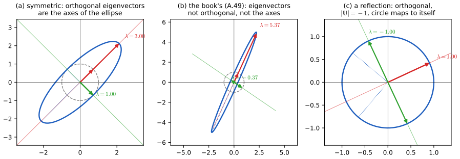
Let \(\bU\) be square with \(\bU^\T\bU=\bI\). Then (a) \(\bU\) is invertible, \(\bU^{-1}=\bU^\T\) and \(\bU\bU^\T=\bI\): the rows are orthonormal too; (b) \(|\bU|=\pm1\), and both signs occur: the book's "\(|\bU|=1\)" is wrong; (c) \(\bU\) preserves lengths and inner products, (A.40)–(A.41). Orthogonal matrices with \(|\bU|=1\) are rotations; those with \(|\bU|=-1\) include a reflection.
Proof
(a) The book's argument multiplies by \(\bU^{-1}\) before knowing that it exists. Instead: \(|\bU^\T||\bU|=|\bI|=1\) and \(|\bU^\T|=|\bU|\) give \(|\bU|^2=1\), so \(|\bU|\ne0\) and \(\bU\) is invertible (Result A.5(f)). Multiplying \(\bU^\T\bU=\bI\) on the right by \(\bU^{-1}\) gives \(\bU^\T=\bU^{-1}\), hence \(\bU\bU^\T=\bU\bU^{-1}=\bI\).
(b) \(|\bU|^2=1\) gives \(|\bU|=\pm1\), not \(+1\). Example: the reflection in a line through the origin at angle \(\theta\), \(\begin{pmatrix}\cos2\theta&\sin2\theta\\ \sin2\theta&-\cos2\theta\end{pmatrix}\), is orthogonal and symmetric with determinant \(-1\) (eigenvalues \(1\) and \(-1\)); simpler still, \(\diag(1,-1)\). For an eigenvector matrix the sign is at our disposal: replacing \(\bu_1\) by \(-\bu_1\) flips it, so one can always choose \(|\bU|=1\), which may be what was meant.
(c) (A.40)–(A.41) are direct, using (A.37). Lengths and angles preserved, so \(\bU\) is a rigid motion fixing the origin: a rotation, or a rotation combined with a reflection. Figure A.S1(c) and a direct computation show a reflection with \(|\bU|=-1\). ∎
Used in the rotated coordinates of a Gaussian, Section 3.2.1, and of a quadratic error surface, Section 7.1.1; rotations in rotary position encodings, Result 12.9.
fig_a_s1. Download: PDF · SVGpp. 614–615 From (A.38),
\[ \bU^\T\bA\bU=\Lam, \tag{A.42} \] \[ \bA=\bU\Lam\bU^\T, \tag{A.43} \] \[ \bA^{-1}=\bU\Lam^{-1}\bU^\T, \tag{A.44} \] \[ \bA=\sum_{i=1}^M\lambda_i\bu_i\bu_i^\T, \tag{A.45} \] \[ \bA^{-1}=\sum_{i=1}^M\frac1{\lambda_i}\bu_i\bu_i^\T, \tag{A.46} \] \[ |\bA|=\prod_{i=1}^M\lambda_i, \tag{A.47} \] \[ \Tr(\bA)=\sum_{i=1}^M\lambda_i. \tag{A.48} \]Result A.14 (diagonalisation and its consequences) pp. 614–615, (A.42)–(A.48)
(a) For a real symmetric matrix, (A.42)–(A.46) hold, (A.44) and (A.46) when every \(\lambda_i\ne0\). More generally any function defined on the eigenvalues acts through them: \(\bA^k=\bU\Lam^k\bU^\T\), and if all \(\lambda_i\ge0\), \(\bA^{1/2}=\bU\Lam^{1/2}\bU^\T\) is the unique symmetric positive semidefinite square root. (b) (A.47) and (A.48) hold for every square matrix, with its complex eigenvalues counted with multiplicity.
Proof
(a) Multiply (A.38) on the left by \(\bU^\T\) for (A.42); multiply (A.42) on the left by \(\bU\) and on the right by \(\bU^\T\) for (A.43), using \(\bU\bU^\T=\bI\). Invert (A.43) with (A.3) and \(\bU^{-1}=\bU^\T\) for (A.44). Writing the products column by column, \(\bU\Lam\bU^\T=\sum_i\lambda_i\bu_i\bu_i^\T\), gives (A.45)–(A.46). Powers: \(\bA^2=\bU\Lam\bU^\T\bU\Lam\bU^\T=\bU\Lam^2\bU^\T\), and so on.
(b) For a symmetric matrix, take the determinant and trace of (A.43): \(|\bU||\Lam||\bU^\T|=|\Lam|\) since \(|\bU|^2=1\), and \(\Tr(\bU\Lam\bU^\T)=\Tr(\Lam\bU^\T\bU)=\Tr\Lam\). For a general matrix use the factorisation \(|\bA-\lambda\bI|=\prod_i(\lambda_i-\lambda)\) of Filling the gap A.3. At \(\lambda=0\) it gives \(|\bA|=\prod_i\lambda_i\). The coefficient of \(\lambda^{M-1}\) on the right is \((-1)^{M-1}\sum_i\lambda_i\); on the left, by (A.10), only the identity permutation reaches degree \(M-1\), through \(\prod_i(A_{ii}-\lambda)\), whose \(\lambda^{M-1}\) coefficient is \((-1)^{M-1}\sum_iA_{ii}\). So \(\Tr\bA=\sum_i\lambda_i\). Checked for a random \(6\times6\) matrix with complex eigenvalues, and the rotation (preset 4 of the demo) has \(|\bA|=1=i\cdot(-i)\) and \(\Tr\bA=0\). ∎
Used in the quadratic error surface in eigen-coordinates and the "trace and determinant" test of Exercise 7.3; the graph Laplacian's spectrum, Result 13.4 and Filling the gap 13.4; the Jacobian determinant of a change of variables, Section 2.4.1.
p. 615 A matrix is positive definite, \(\bA\succ0\), if \(\bw^\T\bA\bw>0\) for every \(\bw\ne\bzero\), and positive semidefinite, \(\bA\succeq0\), if \(\bw^\T\bA\bw\ge0\) for every \(\bw\). The book says this is equivalent to all \(\lambda_i>0\) (respectively \(\ge0\)), and warns that positive entries are not enough, with the example
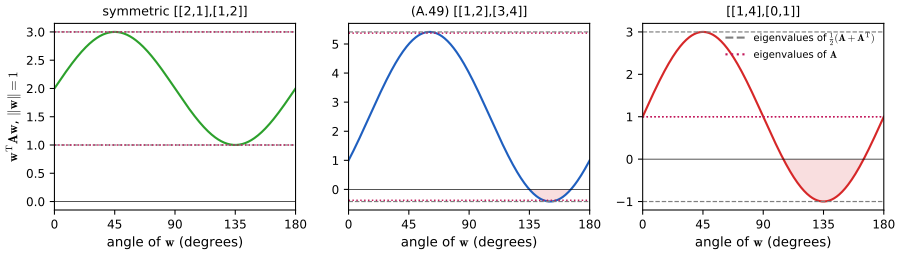
\[ \begin{pmatrix}1&2\\3&4\end{pmatrix}, \tag{A.49} \]whose eigenvalues are \(\lambda_1\simeq5.37\) and \(\lambda_2\simeq-0.37\). The equivalence is proved for symmetric matrices, but (A.49) is not symmetric, and for non-symmetric matrices the eigenvalue test fails.
Result A.15 (positive definiteness) p. 615, (A.49)
- (a) Symmetric \(\bA\): \(\lambda_{\min}\|\bw\|^2\le\bw^\T\bA\bw\le\lambda_{\max}\|\bw\|^2\), with equality along the corresponding eigenvectors. Hence \(\bA\succ0\iff\) all \(\lambda_i>0\), and \(\bA\succeq0\iff\) all \(\lambda_i\ge0\iff\bA=\bB^\T\bB\) for some \(\bB\).
- (b) Any square \(\bA\): \(\bw^\T\bA\bw=\bw^\T\bA_s\bw\) with the symmetric part \(\bA_s=\tfrac12(\bA+\bA^\T)\), so \(\bA\succ0\iff\bA_s\succ0\iff\) the eigenvalues of \(\bA_s\) are positive. The eigenvalues of \(\bA\) itself do not decide: if \(\bA\succ0\) then every real eigenvalue of \(\bA\) is positive and every complex one has positive real part, but the converse fails.
- (c) The book's example: (A.49) has eigenvalues \((5\pm\sqrt{33})/2=5.372,\ -0.372\) and symmetric part \(\begin{pmatrix}1&2.5\\2.5&4\end{pmatrix}\) with eigenvalues \((5\pm\sqrt{34})/2=5.415,\ -0.415\). Its conclusion (not positive definite) is right, by the necessary condition in (b). But \(\begin{pmatrix}1&4\\0&1\end{pmatrix}\) has both eigenvalues equal to 1 and still \(\bw^\T\bA\bw=-2\) at \(\bw=(1,-1)^\T\).
Proof
(a) Expand \(\bw=\sum_ic_i\bu_i\) with \(c_i=\bu_i^\T\bw\) (Result A.12). By (A.45) and orthonormality, \(\bw^\T\bA\bw=\sum_i\lambda_ic_i^2\) and \(\|\bw\|^2=\sum_ic_i^2\); bounding each \(\lambda_i\) between \(\lambda_{\min}\) and \(\lambda_{\max}\) gives the inequalities. If all \(\lambda_i>0\), \(\sum_i\lambda_ic_i^2>0\) unless every \(c_i=0\); conversely \(\bw=\bu_i\) gives \(\bu_i^\T\bA\bu_i=\lambda_i\), which must be positive. If all \(\lambda_i\ge0\), \(\bB=\Lam^{1/2}\bU^\T\) gives \(\bB^\T\bB=\bA\); and any \(\bB^\T\bB\) has \(\bw^\T\bB^\T\bB\bw=\|\bB\bw\|^2\ge0\).
(b) \(\bw^\T\bA\bw\) is a scalar, so it equals its transpose \(\bw^\T\bA^\T\bw\), hence their average \(\bw^\T\bA_s\bw\). The skew part \(\tfrac12(\bA-\bA^\T)\) is invisible to quadratic forms. If \(\bA\succ0\) and \(\bA\bu=\lambda\bu\) with \(\bu=\ba+i\bb\) (\(\ba,\bb\) real, not both zero), then \((\bu^\star)^\T\bA\bu=\lambda\|\bu\|^2\), and the real part of the left side is \(\ba^\T\bA\ba+\bb^\T\bA\bb>0\) (the cross terms \(i(\ba^\T\bA\bb-\bb^\T\bA\ba)\) are imaginary). So \(\mathrm{Re}\,\lambda>0\).
(c) The characteristic polynomial of (A.49) is \(\lambda^2-5\lambda-2\), of its symmetric part \(\lambda^2-5\lambda-2.25\). For \(\begin{pmatrix}1&4\\0&1\end{pmatrix}\), \(\bw^\T\bA\bw=w_1^2+4w_1w_2+w_2^2\), equal to \(1-4+1=-2\) at \((1,-1)\); its symmetric part has eigenvalues \(3\) and \(-1\). Figure A.S2 plots \(\bw^\T\bA\bw\) on the unit circle for these matrices: its range is always the interval between the eigenvalues of \(\bA_s\). All checked numerically. The upper bound in (a), maximised over unit vectors, is the Rayleigh quotient of the companion Toolkit, Section 3.4. ∎
fig_a_s2. Download: PDF · SVGUsed in the test for a minimum, Exercise 7.2; positive definite covariance and kernel matrices, Section 3.2.1; the outer-product Hessian, which is always positive semidefinite, Result 8.5.
p. 615 Finally the book defines the condition number of a matrix as
\[ \mathrm{CN}=\left(\frac{\lambda_{\max}}{\lambda_{\min}}\right)^{1/2}. \tag{A.50} \]Filling the gap A.4: two condition numbers p. 615, (A.50); p. 228
Chapter 7 (p. 228, and Definition 7.2 of this course) calls \(\lambda_{\max}/\lambda_{\min}\) the condition number of the Hessian; (A.50) takes its square root. Both quantities are meaningful; they answer different questions, and (A.50) needs a symmetric positive definite matrix to make sense.
Derivation
The standard condition number. For any invertible matrix, \(\kappa(\bA)=\|\bA\|\,\|\bA^{-1}\|=\sigma_{\max}/\sigma_{\min}\) in the Euclidean norm, the ratio of the largest to the smallest singular value. It bounds how much a relative error in \(\bb\) can be amplified in the solution of \(\bA\bx=\bb\): \(\|\delta\bx\|/\|\bx\|\le\kappa\|\delta\bb\|/\|\bb\|\). For a symmetric positive definite \(\bH\), the singular values are the eigenvalues and \(\kappa(\bH)=\lambda_{\max}/\lambda_{\min}\): this is the number that sets the speed of gradient descent in Section 7.3.
The book's (A.50). For symmetric positive definite \(\bH\), the contour \(\bw^\T\bH\bw=1\) is an ellipse (ellipsoid) with semi-axes of length \(\lambda_i^{-1/2}\) along \(\bu_i\) (set \(\bw=r\bu_i\) in \(\sum_i\lambda_ic_i^2=1\)). So \((\lambda_{\max}/\lambda_{\min})^{1/2}\) is the ratio of the longest to the shortest axis, i.e. how elongated the error contours look, and it equals \(\kappa(\bH^{1/2})\). For \(\bH=\begin{pmatrix}4&1\\1&0.5\end{pmatrix}\) the axis ratio of the contour, measured directly, is \(4.266\) against \((\lambda_{\max}/\lambda_{\min})^{1/2}=4.266\), while the library's condition number is \(18.20=\lambda_{\max}/\lambda_{\min}\). When reading "condition number" in the book, check which one is meant; this course uses \(\lambda_{\max}/\lambda_{\min}\) throughout (as in Filling the gap 4.4, where it is the squared condition number of the design matrix).
Used in the convergence rate of gradient descent, Section 7.3 and the step size demo; ill-conditioning of the normal equations, Section 4.1.4; Langevin sampling of an elongated Gaussian, Result 14.16.
Appendix B. Calculus of Variations
See also the companion course, Toolkit, Section 2.2 (optimising over distributions) and Filling the gap 6.6 (an Euler–Lagrange equation).
p. 617 A function takes a number and returns a number; a functional \(F[y]\) takes a whole function \(y(x)\) and returns a number. Examples: the length of the curve \(y(x)\) between two points, and the entropy \(\mathrm{H}[p]=-\int p(x)\ln p(x)\,\d x\) of a density. The calculus of variations finds the functions that make a functional stationary; it shows, for instance, that the shortest path between two points is a straight line and that, among densities with a given variance, the Gaussian has the largest entropy.
B.1 Functionals and the functional derivative
pp. 617–618 An ordinary derivative can be defined by expanding in a small change \(\epsilon\),
\[ y(x+\epsilon)=y(x)+\frac{\d y}{\d x}\epsilon+O(\epsilon^2), \tag{B.1} \]and partial derivatives by
\[ y(x_1+\epsilon_1,\dots,x_D+\epsilon_D)=y(x_1,\dots,x_D)+\sum_{i=1}^D\frac{\partial y}{\partial x_i}\epsilon_i+O(\epsilon^2). \tag{B.2} \]Definition B.1 (functional derivative) p. 618, (B.3)
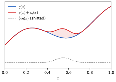
Perturb \(y\) by \(\epsilon\eta(x)\), with \(\eta\) any smooth function that vanishes where \(y\) is held fixed (Figure B.1). The functional derivative \(\delta F/\delta y(x)\) is the function for which
\[ F[y(x)+\epsilon\eta(x)]=F[y(x)]+\epsilon\int\frac{\delta F}{\delta y(x)}\eta(x)\,\d x+O(\epsilon^2) \tag{B.3} \]for every such \(\eta\). Equivalently, \(\dfrac{\d}{\d\epsilon}F[y+\epsilon\eta]\Big|_{\epsilon=0}=\displaystyle\int\fd{F}{y(x)}\,\eta(x)\,\d x\): the directional derivative of \(F\) in the direction \(\eta\) is an integral against a fixed function, the gradient of \(F\).
fig_b_1. Download: PDF · SVGFilling the gap B.1: (B.3) as the limit of (B.2), and how to compute a functional derivative p. 618
The book calls (B.3) "a natural extension of (B.2)" in which \(F\) depends on infinitely many variables, the values \(y(x)\). The analogy can be made exact, and it gives a practical recipe.
Derivation
Discretise. On a grid \(x_k=x_0+k\Delta\), a functional \(F[y]=\int G(y(x),x)\,\d x\) becomes the ordinary function \(F_\Delta(y_0,\dots,y_K)=\sum_kG(y_k,x_k)\Delta\) of the values \(y_k=y(x_k)\). Then by (B.2) \[ F_\Delta(\by+\epsilon\boldsymbol\eta)-F_\Delta(\by)=\epsilon\sum_k\frac{\partial F_\Delta}{\partial y_k}\eta_k+O(\epsilon^2)=\epsilon\sum_k\Big(\frac{1}{\Delta}\frac{\partial F_\Delta}{\partial y_k}\Big)\eta_k\,\Delta+O(\epsilon^2), \] and the sum is a Riemann sum for (B.3). So \(\delta F/\delta y(x_k)=\lim\frac{1}{\Delta}\partial F_\Delta/\partial y_k\): the functional derivative is the gradient with respect to the grid values, divided by the grid spacing. (A component of the gradient is "per grid point"; the functional derivative is "per unit length".) A numerical test confirms it for \(F[p]=\int p\ln p\,\d x\) on a grid of 601 points.
Recipe. Compute \(\frac{\d}{\d\epsilon}F[y+\epsilon\eta]\) at \(\epsilon=0\), rearrange it (integrating by parts if derivatives of \(\eta\) appear) into the form \(\int(\cdots)\eta(x)\,\d x\), and read off the bracket. Examples:
- \(F=\int y^2\,\d x\): \(\frac{\d}{\d\epsilon}\int(y+\epsilon\eta)^2=\int2y\eta\), so \(\delta F/\delta y=2y\).
- \(F=\int p\ln p\,\d x\): \(\delta F/\delta p=\ln p+1\) (the entropy is minus this functional).
- \(F=\iint k(x,x')y(x)y(x')\,\d x\,\d x'\): \[\delta F/\delta y(x)=\int\{k(x,x')+k(x',x)\}y(x')\,\d x'\], the continuous analogue of \(\nabla(\by^\T\bK\by)=(\bK+\bK^\T)\by\) in Result A.7.
- \(F=y(x_0)\) (evaluation at a point): \(\frac{\d}{\d\epsilon}F=\eta(x_0)\), so \(\delta F/\delta y(x)\) is the Dirac delta \(\delta(x-x_0)\), not an ordinary function. The definition (B.3) covers only functionals whose first variation is an integral against a function, which includes every integral functional used in the book.
B.2 Stationary functions
p. 618 \(F\) is stationary at \(y\) if the first-order term vanishes for every perturbation,
\[ \int\frac{\delta F}{\delta y(x)}\eta(x)\,\d x=0, \tag{B.4} \]and the book argues, with perturbations concentrated near a single point, that the functional derivative must then vanish everywhere. This is the fundamental lemma of the calculus of variations; it needs the functional derivative to be continuous.
Result B.1 (fundamental lemma) p. 618, (B.4)
Let \(h\) be continuous on an interval \((a,b)\). If \(\int_a^bh(x)\eta(x)\,\d x=0\) for every infinitely differentiable \(\eta\) that vanishes outside a closed subinterval of \((a,b)\), then \(h(x)=0\) for all \(x\in(a,b)\). Applied to \(h=\delta F/\delta y\), (B.4) implies \(\delta F/\delta y(x)=0\) everywhere.
Proof
Suppose \(h(\hat x)\ne0\) for some \(\hat x\); replacing \(h\) by \(-h\) if needed, \(h(\hat x)>0\). By continuity there is \(\delta>0\) with \(h(x)>h(\hat x)/2\) on \((\hat x-\delta,\hat x+\delta)\subset(a,b)\). Take the smooth bump \(\eta(x)=\exp\{-1/(\delta^2-(x-\hat x)^2)\}\) for \(|x-\hat x|\lt\delta\) and \(\eta=0\) elsewhere: it is infinitely differentiable, non-negative, and positive on the open interval. Then \(\int h\eta\,\d x\ge\tfrac12h(\hat x)\int\eta\,\d x>0\), a contradiction. (Continuity matters: a function that is non-zero at a single point integrates to zero against every \(\eta\).) ∎
B.3 The Euler–Lagrange equations
pp. 618–619 Consider a functional of \(y\), its derivative \(y'\) and \(x\),
\[ F[y]=\int G\big(y(x),y'(x),x\big)\,\d x, \tag{B.5} \]with \(y\) fixed at the ends of the interval. A first-order expansion gives
\[ F[y+\epsilon\eta]=F[y]+\epsilon\int\left\{\frac{\partial G}{\partial y}\eta(x)+\frac{\partial G}{\partial y'}\eta'(x)\right\}\d x+O(\epsilon^2), \tag{B.6} \]and integration by parts of the second term turns it into
\[ F[y+\epsilon\eta]=F[y]+\epsilon\int\left\{\frac{\partial G}{\partial y}-\frac{\d}{\d x}\left(\frac{\partial G}{\partial y'}\right)\right\}\eta(x)\,\d x+O(\epsilon^2), \tag{B.7} \]from which stationarity gives the Euler–Lagrange equation
\[ \frac{\partial G}{\partial y}-\frac{\d}{\d x}\left(\frac{\partial G}{\partial y'}\right)=0. \tag{B.8} \]Result B.2 (Euler–Lagrange equation) pp. 618–619, (B.5)–(B.8)
Let \(G(y,p,x)\) have continuous second partial derivatives, and let \(y\) be twice continuously differentiable on \([a,b]\) with \(y(a)\) and \(y(b)\) prescribed. If \(F\) in (B.5) is stationary at \(y\) among such functions, then (B.8) holds on \((a,b)\); that is, \(\delta F/\delta y=\partial G/\partial y-\frac{\d}{\d x}\partial G/\partial y'\). If instead the value at an end, say \(y(b)\), is left free, the stationary function satisfies (B.8) together with the natural boundary condition \(\partial G/\partial y'=0\) at \(x=b\).
Proof
(B.6). Admissible perturbations are \(C^2\) functions \(\eta\) with \(\eta(a)=\eta(b)=0\), so that \(y+\epsilon\eta\) keeps the boundary values. Fix such an \(\eta\) and let \(\phi(\epsilon)=F[y+\epsilon\eta]\). Because \(G\) has continuous second derivatives and \(y,\eta\) range over a bounded set on the closed interval, we may differentiate under the integral sign: \(\phi'(0)=\int_a^b\{G_y\eta+G_{y'}\eta'\}\,\d x\), where \(G_y\) and \(G_{y'}\) are evaluated at \((y(x),y'(x),x)\), and \(\phi''\) is bounded, which gives the \(O(\epsilon^2)\) remainder in (B.6).
(B.7). \(x\mapsto G_{y'}(y(x),y'(x),x)\) is continuously differentiable (chain rule: \(\frac{\d}{\d x}G_{y'}=G_{y'y}y'+G_{y'y'}y''+G_{y'x}\), all continuous). Integrating by parts, \[ \int_a^bG_{y'}\eta'\,\d x=\Big[G_{y'}\eta\Big]_a^b-\int_a^b\frac{\d}{\d x}\big(G_{y'}\big)\eta\,\d x, \] and the boundary term vanishes because \(\eta(a)=\eta(b)=0\). This gives (B.7) and identifies the functional derivative in the sense of (B.3).
(B.8). Stationarity means \(\phi'(0)=0\) for every admissible \(\eta\), in particular for every smooth \(\eta\) vanishing near \(a\) and \(b\). The bracket in (B.7) is continuous, so the fundamental lemma (Result B.1) makes it vanish on \((a,b)\).
Free end. If \(y(b)\) is free, perturbations with \(\eta(b)\ne0\) are allowed. Those with \(\eta(b)=0\) still give (B.8); then for a general \(\eta\) only the boundary term survives, \(G_{y'}(b)\eta(b)=0\), and choosing \(\eta(b)\ne0\) gives \(G_{y'}=0\) at \(b\). Checked numerically: for \(G=y^2+y'^2\) and a function that is not stationary, the first variation computed by finite differences equals \(\int(G_y-\frac{\d}{\d x}G_{y'})\eta\,\d x\) to six digits. ∎
p. 619 The book's example is
\[ G=y(x)^2+\big(y'(x)\big)^2, \tag{B.9} \]for which (B.8) reads \(2y-\frac{\d}{\d x}(2y')=0\), i.e.
\[ y(x)-\frac{\d^2y}{\d x^2}=0, \tag{B.10} \]to be solved with the boundary conditions.
Result B.3 (solving (B.10), and when a stationary function is a minimum) p. 619, (B.9), (B.10)
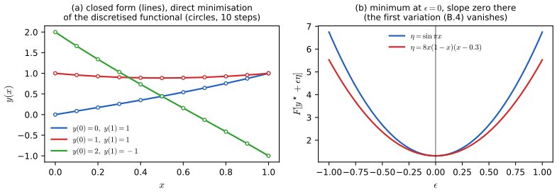
(a) On \([0,1]\) with \(y(0)=a\), \(y(1)=b\), the solution of (B.10) is \(y^\star(x)=\dfrac{a\sinh(1-x)+b\sinh x}{\sinh1}\), and it is the unique global minimiser of \(F[y]=\int_0^1(y^2+y'^2)\,\d x\); the minimum value is \(F[y^\star]=\big[y^\star y^{\star\prime}\big]_0^1\), which is \(\coth1=1.3130\) for \(a=0\), \(b=1\). (b) More generally, if \(G(y,p,x)\) is convex in \((y,p)\) for each \(x\), every solution of the Euler–Lagrange equation with the prescribed boundary values is a global minimiser of \(F\).
Proof
(a) The general solution of \(y''=y\) is \(y=c_1\sinh x+c_2\sinh(1-x)\) (two independent solutions of a second-order linear equation); the boundary values give \(c_2\sinh1=a\) and \(c_1\sinh1=b\). For any admissible \(\eta\) (zero at both ends), \[ F[y^\star+\eta]-F[y^\star]=2\int_0^1\big(y^\star\eta+y^{\star\prime}\eta'\big)\d x+\int_0^1\big(\eta^2+\eta'^2\big)\d x. \] The first integral is \(2\int(y^\star-y^{\star\prime\prime})\eta\,\d x=0\) after integrating by parts, so the difference is \(\int(\eta^2+\eta'^2)\,\d x>0\) unless \(\eta\equiv0\): a strict global minimum. For the value, integrate \(\int y'^2=[yy']-\int yy''\) and use \(y''=y\): \(F[y^\star]=[y^\star y^{\star\prime}]_0^1\); with \(a=0,b=1\), \(y^{\star\prime}(1)=\cosh1/\sinh1\).
(b) A convex differentiable function lies above its tangent plane: \[G(y+\eta,y'+\eta',x)\ge G(y,y',x)+G_y\eta+G_{y'}\eta'\]. Integrate: \[F[y+\eta]\ge F[y]+\int(G_y\eta+G_{y'}\eta')\,\d x=F[y]\], the last integral being zero for a solution of (B.8) by (B.7). Example (a) is the case \(G=y^2+p^2\).
Numerical confirmation (Figure B.S1). Minimising a discretised version of \(F\) over the values of \(y\) at the interior grid points (a linear system, since \(F\) is quadratic) reproduces \(y^\star\) with error \(4.4\times10^{-5}\), \(1.1\times10^{-5}\), \(2.8\times10^{-6}\) for 10, 20 and 40 steps, the factor 4 of a second-order method, without ever writing down (B.10). Along any line \(y^\star+\epsilon\eta\), \(F\) is a parabola in \(\epsilon\) with its minimum at \(\epsilon=0\). ∎
fig_b_s1. Download: PDF · SVGThe shortest path. The length of the graph of \(y\) from \((0,0)\) to \((1,1)\) is \(F[y]=\int_0^1\sqrt{1+y'^2}\,\d x\). Here \(G\) does not depend on \(y\), so (B.8) says \(\frac{\d}{\d x}\big(y'/\sqrt{1+y'^2}\big)=0\): \(y'/\sqrt{1+y'^2}\) is constant, so \(y'\) is constant and the path is the straight line \(y=x\). Since \(\sqrt{1+p^2}\) is convex in \(p\), Result B.3(b) makes it the global minimum, of length \(\sqrt2\). Minimising the length of a 40-segment polygonal path from a wiggly start gives \(\sqrt2\) to \(10^{-11}\) (Figure B.S2(b)).
p. 619 Integrands without derivatives. If \(G=G(y,x)\) does not involve \(y'\), then \(\delta F/\delta y(x)=\partial G/\partial y\) and stationarity is the pointwise condition \(\partial G/\partial y(x)=0\) for every \(x\): the problem splits into one ordinary minimisation per value of \(x\). The book's main use of this is the regression function: \[\E[L]=\iint\{f(\bx)-t\}^2p(\bx,t)\,\d\bx\,\d t=\int G(f(\bx),\bx)\,\d\bx\] with \(G(f,\bx)=\int(f-t)^2p(\bx,t)\,\d t\), and \(\partial G/\partial f=2\int(f-t)p(\bx,t)\,\d t=0\) gives \(f^\star(\bx)=\E[t\given\bx]\) (4.36)–(4.37).
Used in the regression function, Result 4.9 (companion: Result 1.18).
B.4 Constraints and several variables
p. 619 When the unknown is a probability density, the normalisation \(\int p=1\) (and possibly moment conditions) must be respected; the book handles this with Lagrange multipliers (Appendix C), which turn the problem into an unconstrained stationarity condition for a modified functional. The prime example is maximum entropy.
Result B.4 (maximum entropy with fixed mean and variance) p. 617, p. 619; Section 2.5.4, (2.93)–(2.97)
Among densities on \(\R\) with \(\int p=1\), \(\int xp\,\d x=\mu\) and \(\int(x-\mu)^2p\,\d x=\sigma^2\), the entropy \(\mathrm{H}[p]=-\int p\ln p\,\d x\) is maximised by \(\N(x\given\mu,\sigma^2)\), uniquely, with \(\mathrm{H}=\tfrac12\ln(2\pi e\sigma^2)\). (Without the variance constraint there is no maximum: the entropy can be made arbitrarily large.)
Proof: the Lagrange route finds it, an inequality proves it
Stationarity. With multipliers \(\lambda_1,\lambda_2,\lambda_3\), make stationary \[ \widetilde F[p]=-\int p\ln p\,\d x+\lambda_1\Big(\int p\,\d x-1\Big)+\lambda_2\Big(\int xp\,\d x-\mu\Big)+\lambda_3\Big(\int(x-\mu)^2p\,\d x-\sigma^2\Big). \] The integrand depends on \(p(x)\) but not on its derivative, so by B.3 the functional derivative is the partial derivative of the integrand: \[-\ln p(x)-1+\lambda_1+\lambda_2x+\lambda_3(x-\mu)^2=0\], so \(p(x)=\exp\{-1+\lambda_1+\lambda_2x+\lambda_3(x-\mu)^2\}\) (2.97). It is normalisable only if \(\lambda_3\lt0\); completing the square, it is a Gaussian with mean \(\mu-\lambda_2/(2\lambda_3)\) and variance \(-1/(2\lambda_3)\). The mean and variance constraints force \(\lambda_2=0\) and \(\lambda_3=-1/(2\sigma^2)\), and normalisation fixes \(\lambda_1\).
It is the maximum. Stationarity alone does not show that. Let \(\varphi=\N(\mu,\sigma^2)\) and let \(p\) satisfy the constraints. Since \(-\ln\varphi(x)=\tfrac12\ln(2\pi\sigma^2)+(x-\mu)^2/(2\sigma^2)\) and \(p\) has variance \(\sigma^2\), \(-\int p\ln\varphi=\tfrac12\ln(2\pi\sigma^2)+\tfrac12=\mathrm{H}[\varphi]\). Hence \[ 0\le\KL(p\,\|\,\varphi)=\int p\ln p-\int p\ln\varphi=-\mathrm{H}[p]+\mathrm{H}[\varphi], \] with equality only if \(p=\varphi\) (Gibbs' inequality). No calculus of variations is needed for this half; see the companion Toolkit, Section 1.2.
Numerical confirmation (Figure B.S2(a)). A generic constrained optimiser, given only the discretised entropy and the three constraints on 161 grid values and started from a flat-topped density, converges to the Gaussian to \(3\times10^{-6}\) and to entropy \(1.4189385\) against \(\tfrac12\ln(2\pi e)=1.4189385\). The Laplace, logistic and uniform densities with the same variance have entropies \(1.347\), \(1.405\) and \(1.242\) nats (closed forms confirmed by quadrature). ∎
Used in Section 2.5.4 (maximum entropy) and Exercise 3.8 (its multivariate version); the discrete case with one multiplier, Result 2.8. Companion: Result 1.21 and Result 2.13.
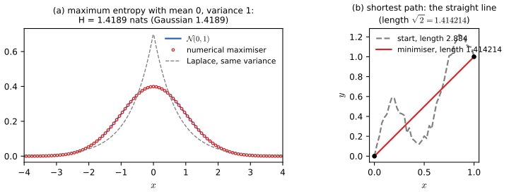
fig_b_s2. Download: PDF · SVGp. 619 The book says the extension to a multi-dimensional variable is "straightforward". Here it is.
Result B.5 (Euler–Lagrange equations in several variables) p. 619
Let \(\Omega\subset\R^D\) be a bounded region with smooth boundary and \(F[y]=\int_\Omega G(y,\nabla y,\bx)\,\d\bx\), with \(y\) prescribed on the boundary \(\partial\Omega\). Write \(p_i\) for the slot of \(G\) that receives \(\partial y/\partial x_i\). Under the smoothness assumptions of Result B.2, a stationary \(y\) satisfies
\[ \frac{\partial G}{\partial y}-\sum_{i=1}^D\frac{\partial}{\partial x_i}\left(\frac{\partial G}{\partial p_i}\right)=0\quad\text{in }\Omega . \]With several unknown functions \(y_1,\dots,y_K\) there is one such equation per function. Example: \(G=\|\nabla y\|^2\) gives Laplace's equation \(\sum_i\partial^2y/\partial x_i^2=0\).
Proof
As in one dimension, \(\frac{\d}{\d\epsilon}F[y+\epsilon\eta]\big|_0=\int_\Omega\{G_y\eta+\sum_iG_{p_i}\partial_i\eta\}\,\d\bx\). The divergence theorem applied to the vector field \(\eta\,(G_{p_1},\dots,G_{p_D})\) gives \[\int_\Omega\sum_iG_{p_i}\partial_i\eta=\oint_{\partial\Omega}\eta\sum_iG_{p_i}n_i\,\d S-\int_\Omega\eta\sum_i\partial_iG_{p_i}\], with \(\bn\) the outward normal; the boundary integral vanishes because \(\eta=0\) on \(\partial\Omega\). The fundamental lemma (with bumps in \(D\) dimensions) finishes the proof. With several functions, perturb one at a time. For \(G=\sum_ip_i^2\), \(G_{p_i}=2\partial_iy\) and the equation is \(-2\sum_i\partial_i^2y=0\). Numerically, on a \(120\times120\) grid the first variation of the discretised Dirichlet energy \(\int\|\nabla y\|^2\) vanishes (to \(2\times10^{-11}\)) at the harmonic function \(x^2-y^2\), but not at \(x^2+y^2\). ∎
Appendix C. Lagrange Multipliers
See also the companion course, Toolkit, Section 2.1 (Lagrange multipliers) and Result 7.3 (KKT conditions and support vectors).
C.1 Equality constraints
p. 621 Lagrange (or undetermined) multipliers find stationary points of a function of several variables under constraints. To maximise \(f(x_1,x_2)\) subject to
\[ g(x_1,x_2)=0, \tag{C.1} \]one could solve the constraint for \(x_2=h(x_1)\) and maximise \(f(x_1,h(x_1))\). This needs an explicit solution of the constraint, which may not exist in closed form, and it treats the variables asymmetrically. The multiplier method avoids both problems. In \(D\) dimensions the constraint \(g(\bx)=0\) is a \((D-1)\)-dimensional surface, and a Taylor expansion along it,
\[ g(\bx+\beps)\simeq g(\bx)+\beps^\T\nabla g(\bx), \tag{C.2} \]shows that \(\nabla g\) is orthogonal to the surface.
Result C.1 (the gradient is normal to a level surface) pp. 621–622, (C.2)
Let \(g\) be continuously differentiable and \(g(\bx)=0\) with \(\nabla g(\bx)\ne\bzero\). (a) If \(\bc(s)\) is a differentiable curve in the surface with \(\bc(0)=\bx\), then \(\nabla g(\bx)^\T\bc'(0)=0\). (b) Conversely, every \(\bv\) with \(\nabla g(\bx)^\T\bv=0\) is the velocity \(\bc'(0)\) of such a curve. So the tangent space of the surface at \(\bx\) is exactly the \((D-1)\)-dimensional subspace orthogonal to \(\nabla g(\bx)\).
Proof
(a) \(g(\bc(s))=0\) for all \(s\); differentiate at \(s=0\) with the chain rule. This is the precise form of the book's argument with "a nearby point \(\bx+\beps\) on the surface": the difference \(\beps\) divided by its length tends to a tangent direction.
(b) Some component of \(\nabla g(\bx)\), say \(\partial g/\partial x_D\), is non-zero. By the implicit function theorem, near \(\bx\) the surface is the graph \(x_D=h(x_1,\dots,x_{D-1})\) of a continuously differentiable \(h\), with \(\partial h/\partial x_j=-(\partial g/\partial x_j)/(\partial g/\partial x_D)\). Given \(\bv\) with \(\nabla g^\T\bv=0\), the curve \[\bc(s)=(x_1+sv_1,\dots,x_{D-1}+sv_{D-1},h(\dots))\] lies on the surface and has last velocity component \(\sum_{j\lt D}(\partial h/\partial x_j)v_j=v_D\), using \(\nabla g^\T\bv=0\). So \(\bc'(0)=\bv\). Without \(\nabla g\ne\bzero\) both the dimension count and (b) can fail (Figure C.S2(a)): the surface need not be smooth there. ∎
p. 622 At a constrained maximum \(\bxs\), \(\nabla f\) must also be normal to the surface (otherwise moving along the surface would increase \(f\)), so \(\nabla f\) and \(\nabla g\) are parallel or anti-parallel:
\[ \nabla f+\lambda\nabla g=\bzero. \tag{C.3} \]With the Lagrangian
\[ L(\bx,\lambda)\equiv f(\bx)+\lambda g(\bx), \tag{C.4} \]\(\nabla_\bx L=\bzero\) is (C.3) and \(\partial L/\partial\lambda=0\) is the constraint: \(D+1\) equations for \(\bxs\) and \(\lambda\). The book adds that "\(\lambda\ne0\)" and that \(\lambda\) can have either sign.
Result C.2 (Lagrange's condition, with its hypothesis) p. 622, (C.3), (C.4)
Let \(f\) and \(g\) be continuously differentiable, and let \(\bxs\) be a local maximum (or minimum) of \(f\) on \(\{g=0\}\). If \(\nabla g(\bxs)\ne\bzero\), there is a unique \(\lambda\) with \(\nabla f(\bxs)+\lambda\nabla g(\bxs)=\bzero\). The multiplier may be zero: \(\lambda=0\) exactly when \(\nabla f(\bxs)=\bzero\), i.e. when an unconstrained stationary point happens to lie on the constraint. Without the hypothesis \(\nabla g(\bxs)\ne\bzero\) the conclusion can fail.
Proof and counterexample
Proof. Let \(\bv\) be tangent (\(\nabla g^\T\bv=0\)) and \(\bc\) a curve in the surface with \(\bc(0)=\bxs\), \(\bc'(0)=\bv\) (Result C.1(b)). The function \(s\mapsto f(\bc(s))\) has a local extremum at \(s=0\), so its derivative \(\nabla f(\bxs)^\T\bv\) is zero. Thus \(\nabla f\) is orthogonal to every vector orthogonal to \(\nabla g\), i.e. \(\nabla f\) lies in the span of \(\nabla g\): \(\nabla f=-\lambda\nabla g\), and \(\lambda=-\nabla f^\T\nabla g/\|\nabla g\|^2\) is unique. Nothing prevents \(\lambda=0\): maximise \(f=-(x_1-0.4)^2-(x_2-0.6)^2\) on \(x_1+x_2=1\); the unconstrained maximum \((0.4,0.6)\) is on the line and \(\lambda=0\) (checked).
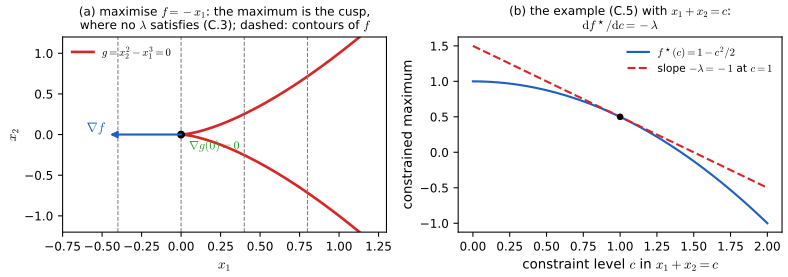
Counterexample without the hypothesis. Maximise \(f=-x_1\) subject to \(g=x_2^2-x_1^3=0\). On the constraint \(x_1=|x_2|^{2/3}\ge0\), so the maximum is at the origin, where the curve has a cusp (Figure C.S2(a)). There \(\nabla f=(-1,0)\) but \(\nabla g=(-3x_1^2,2x_2)=\bzero\), so \(\nabla f+\lambda\nabla g=(-1,0)\ne\bzero\) for every \(\lambda\). The Lagrangian equations \(-1-3\lambda x_1^2=0\), \(2\lambda x_2=0\), \(x_2^2=x_1^3\) have no solution at all: the method silently misses the true maximum. In practice one therefore also inspects the points where \(\nabla g=\bzero\). (The toolkit's version, Result T.4, states the hypothesis as linear independence of the constraint gradients.) ∎
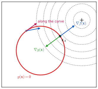
fig_c_1. Download: PDF · SVGpp. 622–623 Example. Find the stationary point of \(f(x_1,x_2)=1-x_1^2-x_2^2\) subject to \(g(x_1,x_2)=x_1+x_2-1=0\) (Figure C.2). The Lagrangian is
\[ L(\bx,\lambda)=1-x_1^2-x_2^2+\lambda(x_1+x_2-1), \tag{C.5} \]and its stationarity conditions are
\[ -2x_1+\lambda=0, \tag{C.6} \] \[ -2x_2+\lambda=0, \tag{C.7} \] \[ x_1+x_2-1=0. \tag{C.8} \]The first two give \(x_1=x_2=\lambda/2\), the third \(\lambda=1\): \((x_1^\star,x_2^\star)=(\tfrac12,\tfrac12)\) and \(f^\star=\tfrac12\). Eliminating instead, \(f(x_1,1-x_1)=1-x_1^2-(1-x_1)^2\) has derivative \(2-4x_1\), zero at \(x_1=\tfrac12\): the same point (both checked, and confirmed by a generic solver).
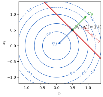
fig_c_2. Download: PDF · SVGFilling the gap C.1: is the stationary point a maximum? pp. 622–623
The Lagrange conditions locate stationary points of \(f\) on the constraint; the book calls \((\tfrac12,\tfrac12)\) "the stationary point" and leaves its nature open.
Derivation
A global argument for concave problems. Suppose \(L(\cdot,\lambda^\star)=f+\lambda^\star g\) is concave in \(\bx\) (for example \(f\) concave and \(g\) affine, as here) and \(\nabla_\bx L(\bxs,\lambda^\star)=\bzero\). A concave function is maximised at any stationary point, so for every feasible \(\bx\) (where \(g(\bx)=0\)), \[ f(\bx)=L(\bx,\lambda^\star)\le L(\bxs,\lambda^\star)=f(\bxs). \] So \((\tfrac12,\tfrac12)\) is the global maximum of \(f\) on the line.
A local test in general. At a stationary point, \(\bxs\) is a strict local maximum on the constraint if \(\bv^\T\nabla_\bx^2L(\bxs,\lambda^\star)\bv\lt0\) for every non-zero tangent \(\bv\) (\(\nabla g^\T\bv=0\)). Note that the Hessian of the Lagrangian, not of \(f\), appears: along a curved constraint, \(\frac{\d^2}{\d s^2}f(\bc(s))=\bc'^\T\nabla^2f\,\bc'+\nabla f^\T\bc''\), and differentiating \(g(\bc(s))=0\) twice gives \(\nabla g^\T\bc''=-\bc'^\T\nabla^2g\,\bc'\), so with \(\nabla f=-\lambda\nabla g\) the second derivative is \(\bc'^\T(\nabla^2f+\lambda\nabla^2g)\bc'\). In the circle example of the demo (preset 2) two of the four stationary points are maxima along the circle and two are minima; the test separates them.
Filling the gap C.2: what the multiplier measures p. 622
The book introduces \(\lambda\) as an auxiliary unknown that can be eliminated. It has a meaning: it is the rate at which the optimal value changes when the constraint is relaxed.
Derivation
Replace the constraint by \(h(\bx)=c\), i.e. \(g(\bx)=h(\bx)-c\), and suppose the maximiser \(\bxs(c)\) and multiplier \(\lambda(c)\) depend differentiably on \(c\). Let \(f^\star(c)=f(\bxs(c))\). Differentiating \(h(\bxs(c))=c\) gives \(\nabla h^\T\frac{\d\bxs}{\d c}=1\). Then, using (C.3), \[ \frac{\d f^\star}{\d c}=\nabla f^\T\frac{\d\bxs}{\d c}=-\lambda\nabla h^\T\frac{\d\bxs}{\d c}=-\lambda . \] (This is the envelope theorem: \(\d f^\star/\d c=\partial L/\partial c\).) In the example with \(x_1+x_2=c\): \(\bxs=(c/2,c/2)\), \(\lambda=c\) and \(f^\star(c)=1-c^2/2\), whose slope at \(c=1\) is \(-1=-\lambda\) (Figure C.S2(b); checked by finite differences). In economics \(\lambda\) is the "shadow price" of the constraint. It also explains why only the product \(\lambda\nabla g\) is meaningful: writing the same constraint as \(2g=0\) halves \(\lambda\).
fig_c_s2. Download: PDF · SVGUsed in maximum likelihood for categorical parameters, Result 3.3, Result 5.13, Result 11.17 and Result 12.11; the discrete maximum entropy distribution, Exercise 2.22; the optimal input of a filter, Filling the gap 10.2 and Exercise 10.1.
C.2 Inequality constraints and the KKT conditions
pp. 623–624 Now maximise \(f(\bx)\) subject to \(g(\bx)\ge0\) (Figure C.3). Either the solution lies inside, \(g>0\), and the constraint is inactive: then \(\nabla f=\bzero\), a stationary point of (C.4) with \(\lambda=0\). Or it lies on the boundary \(g=0\) and is active: then (C.3) holds, and since \(f\) is maximal only if its gradient points out of the feasible region, \(\nabla f=-\lambda\nabla g\) with \(\lambda>0\). In both cases \(\lambda g(\bx)=0\). Hence the conditions
\[ g(\bx)\ge0, \tag{C.9} \] \[ \lambda\ge0, \tag{C.10} \] \[ \lambda g(\bx)=0, \tag{C.11} \]together with \(\nabla_\bx L=\bzero\): the Karush–Kuhn–Tucker (KKT) conditions (Karush, 1939; Kuhn and Tucker, 1951). (C.11) is called complementary slackness: at most one of \(\lambda\) and \(g\) is non-zero.
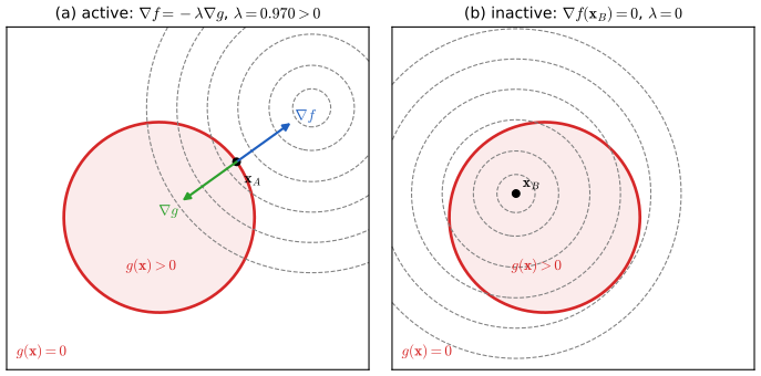
fig_c_3. Download: PDF · SVGResult C.3 (the KKT conditions are necessary) pp. 623–624, (C.9)–(C.11)
Let \(f,g\) be continuously differentiable and \(\bxs\) a local maximum of \(f\) on \(\{g\ge0\}\). If either \(g(\bxs)>0\), or \(g(\bxs)=0\) and \(\nabla g(\bxs)\ne\bzero\), then there is \(\lambda\) with \(\nabla f(\bxs)+\lambda\nabla g(\bxs)=\bzero\) and (C.9)–(C.11). To minimise \(f\) subject to \(g\ge0\), the conditions are the same with \(L=f-\lambda g\) (still \(\lambda\ge0\)).
Proof
Inactive case. If \(g(\bxs)>0\), continuity gives \(g>0\) on a neighbourhood, so \(\bxs\) is a local maximum of \(f\) without constraints: \(\nabla f(\bxs)=\bzero\). Take \(\lambda=0\); (C.9)–(C.11) hold.
Active case. If \(g(\bxs)=0\), then \(\bxs\) is in particular a local maximum on the surface \(g=0\), so Result C.2 gives \(\lambda\) with \(\nabla f=-\lambda\nabla g\), and (C.11) holds because \(g=0\). For the sign, step into the feasible region along \(\nabla g\): \(\bx(s)=\bxs+s\nabla g(\bxs)\), \(s>0\). Then \(g(\bx(s))=s\|\nabla g\|^2+o(s)>0\) for small \(s\), so \(\bx(s)\) is feasible, and \[ f(\bx(s))-f(\bxs)=s\,\nabla f^\T\nabla g+o(s)=-\lambda s\|\nabla g\|^2+o(s). \] This must be \(\le0\) for small \(s>0\) (local maximum), which forces \(\lambda\ge0\). This is the precise content of "the gradient of \(f\) is oriented away from the region \(g>0\)".
Minimisation. Minimising \(f\) is maximising \(-f\): \(-\nabla f+\lambda\nabla g=\bzero\) with \(\lambda\ge0\), i.e. \(\bx\) is stationary for \(f-\lambda g\). Checked: minimising \((x_1-2)^2+(x_2-1)^2\) over the unit disc gives \(\lambda=\sqrt5-1>0\). ∎
Result C.4 (the KKT conditions are sufficient for concave problems) p. 624
If \(f\) and \(g\) are concave (so the feasible set \(\{g\ge0\}\) is convex) and \((\bxs,\lambda^\star)\) satisfy \(\nabla f(\bxs)+\lambda^\star\nabla g(\bxs)=\bzero\) and (C.9)–(C.11), then \(\bxs\) is a global maximum of \(f\) on \(\{g\ge0\}\).
Proof
Since \(\lambda^\star\ge0\), \(L(\cdot,\lambda^\star)=f+\lambda^\star g\) is concave, and it is stationary at \(\bxs\), so it is maximised there. For any feasible \(\bx\), using \(\lambda^\star g(\bx)\ge0\) and then (C.11), \[ f(\bx)\le f(\bx)+\lambda^\star g(\bx)=L(\bx,\lambda^\star)\le L(\bxs,\lambda^\star)=f(\bxs)+\lambda^\star g(\bxs)=f(\bxs). \] Each KKT condition is used exactly once. Without concavity the KKT conditions are only necessary: they also hold at local maxima, at some minima along the boundary, and at saddle points. ∎
Result C.5 (a worked inequality example) Section C (our example)
Maximise \(f(\bx)=-(x_1-a)^2-(x_2-a)^2\) subject to \(g(\bx)=1-x_1^2-x_2^2\ge0\), for \(a\ge0\). The solution is
\[ \bxs=\begin{cases}(a,a), & \lambda^\star=0,\ \text{if } a\le1/\sqrt2,\\ (1,1)/\sqrt2, & \lambda^\star=\sqrt2\,a-1>0,\ \text{if } a>1/\sqrt2.\end{cases} \]Derivation
Stationarity of \(L=f+\lambda g\): \(-2(\bx-a\one)-2\lambda\bx=\bzero\), so \(\bx=a\one/(1+\lambda)\). If \(\lambda=0\), \(\bx=(a,a)\), which satisfies (C.9) only if \(2a^2\le1\). If \(\lambda>0\), (C.11) requires \(g=0\): \(\|\bx\|=\sqrt2a/(1+\lambda)=1\), so \(\lambda=\sqrt2a-1\), which satisfies (C.10) only if \(a\ge1/\sqrt2\). So for every \(a\) exactly one case applies, and since \(f\) and \(g\) are concave, Result C.4 says it is the global maximum. At the switch \(a=1/\sqrt2\) both \(g\) and \(\lambda\) vanish together. A generic solver agrees for \(a\in\{0.3,0.6,0.9,1.5,2.2\}\), and the KKT residuals are below \(10^{-6}\) (Figure C.S1). ∎
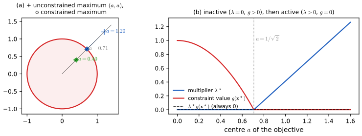
fig_c_s1. Download: PDF · SVGUsed in the equivalence of a penalty and a constraint (weight decay and the lasso), Result 9.6 and Exercise 9.5; the bound \(a_{nm}\le1\) on attention weights, Exercise 12.1. Companion: support vector machines, Result 7.3.
C.3 Several constraints
p. 624 To maximise \(f(\bx)\) subject to \(g_j(\bx)=0\) (\(j=1,\dots,J\)) and \(h_k(\bx)\ge0\) (\(k=1,\dots,K\)), introduce multipliers \(\{\lambda_j\}\) and \(\{\mu_k\}\) and the Lagrangian
\[ L\big(\bx,\{\lambda_j\},\{\mu_k\}\big)=f(\bx)+\sum_{j=1}^J\lambda_jg_j(\bx)+\sum_{k=1}^K\mu_kh_k(\bx), \tag{C.12} \]to be made stationary in \(\bx\) subject to \(\mu_k\ge0\) and \(\mu_kh_k(\bx)=0\) for every \(k\).
Result C.6 (KKT conditions with several constraints) p. 624, (C.12)
(a) Necessity. Let \(\bxs\) be a local maximum, all functions continuously differentiable, and let the gradients of the equality constraints and of the active inequality constraints (those with \(h_k(\bxs)=0\)) be linearly independent (the linear independence constraint qualification). Then there are unique \(\lambda_j\) and \(\mu_k\ge0\) with \(\nabla_\bx L=\bzero\), \(g_j(\bxs)=0\), \(h_k(\bxs)\ge0\) and \(\mu_kh_k(\bxs)=0\). (b) Sufficiency. If \(f\) and every \(h_k\) are concave and every \(g_j\) is affine, any point satisfying these conditions is a global maximum.
Proof (sufficiency in full, necessity in outline)
(b) With the multipliers fixed, \(L\) is concave in \(\bx\) (the \(\lambda_jg_j\) are affine whatever the sign of \(\lambda_j\), and \(\mu_k\ge0\) keeps \(\mu_kh_k\) concave), so it is maximised at its stationary point \(\bxs\). For feasible \(\bx\): \[f(\bx)\le f(\bx)+\sum_j\lambda_jg_j(\bx)+\sum_k\mu_kh_k(\bx)=L(\bx)\le L(\bxs)=f(\bxs)\], where the first step uses \(g_j(\bx)=0\) and \(\mu_kh_k(\bx)\ge0\), and the last uses \(g_j(\bxs)=0\) and \(\mu_kh_k(\bxs)=0\).
(a) Inactive inequalities play no role near \(\bxs\) (set \(\mu_k=0\)). Treat the active ones as equalities first: by the several-constraint version of Result C.2 (its proof with the implicit function theorem for \(J+|A|\) independent gradients, as in the companion Toolkit, Result T.4), \(\nabla f\) is a combination of the constraint gradients, uniquely by independence. For the sign of \(\mu_k\), use independence to find a direction \(\bv\) with \(\nabla g_j^\T\bv=0\) for all \(j\), \(\nabla h_k^\T\bv=1\) and \(\nabla h_l^\T\bv=0\) for the other active \(l\); a curve leaving \(\bxs\) with velocity \(\bv\) can be chosen to stay on the other constraints (implicit function theorem) and enters \(h_k>0\), so it is feasible, and \(f\) cannot increase along it: \(0\ge\nabla f^\T\bv=-\mu_k\). Full details: Nocedal and Wright (1999), Chapter 12. ∎
Result C.7 (projection onto the probability simplex, and weak duality) p. 624 (our examples)
(a) The point of the simplex \(\{\bx:\sum_kx_k=1,\ x_k\ge0\}\) closest to \(\by\in\R^K\) is \(x_k=\max(y_k-\tau,0)\), where \(\tau\) is the unique number making the \(x_k\) sum to one. Its multipliers are \(\nu=-2\tau\) for the equality and \(\mu_k=2\max(\tau-y_k,0)\) for the inequalities. (b) For the example (C.5), the dual function \(q(\lambda)=\max_\bx L(\bx,\lambda)=1-\lambda+\lambda^2/2\) satisfies \(q(\lambda)\ge f^\star=\tfrac12\) for every \(\lambda\), with equality at \(\lambda=1\).
Derivation
(a) This is a minimisation (of a convex function under affine constraints), so use \(L=\|\bx-\by\|^2-\nu(\sum_kx_k-1)-\sum_k\mu_kx_k\) with \(\mu_k\ge0\). Stationarity: \(2(x_k-y_k)-\nu-\mu_k=0\). Write \(\tau=-\nu/2\). If \(x_k>0\), complementary slackness gives \(\mu_k=0\) and \(x_k=y_k-\tau\), which requires \(y_k>\tau\). If \(x_k=0\), \(\mu_k=2(\tau-y_k)\ge0\) requires \(y_k\le\tau\). Both cases say \(x_k=\max(y_k-\tau,0)\) and \(\mu_k=2\max(\tau-y_k,0)\). The map \(\tau\mapsto\sum_k\max(y_k-\tau,0)\) is continuous, strictly decreasing where positive, and runs from \(+\infty\) to 0, so exactly one \(\tau\) gives sum 1. Convexity makes the KKT point the global minimum (Result C.6(b), applied to \(-\|\bx-\by\|^2\)). For \(\by=(0.9,0.4,-0.3,0.2,1.1)\): \(\tau=0.5\), \(\bx=(0.4,0,0,0,0.6)\), \(\boldsymbol\mu=(0,0.2,1.6,0.6,0)\); a generic solver agrees and \(\mu_kx_k=0\) for every \(k\). Coordinates below the threshold are set exactly to zero, which is why this projection is used as a sparse alternative to the softmax (sparsemax; Martins and Astudillo, 2016).
(b) For any \(\lambda\) and any feasible \(\bx\), \(L(\bx,\lambda)=f(\bx)\), so \(q(\lambda)\ge f(\bx)\); taking the best feasible \(\bx\), \(q(\lambda)\ge f^\star\) (weak duality; for inequality constraints the same holds for every \(\lambda\ge0\), since then \(\lambda g(\bx)\ge0\)). In the example, \(L\) is maximised at \(x_1=x_2=\lambda/2\), giving \(q(\lambda)=1-\lambda+\lambda^2/2\), whose minimum over \(\lambda\) is \(q(1)=\tfrac12=f^\star\): the bound is tight (strong duality, which holds for concave problems with affine constraints) and the minimising \(\lambda\) is the Lagrange multiplier. This is confirmed by maximising \(L\) numerically for 26 values of \(\lambda\). Solving the dual instead of the primal problem is how support vector machines are trained (companion Result 7.3). ∎
p. 624 The book closes by noting that constrained functional problems are handled the same way; Result B.4 (maximum entropy with three multipliers) is the example used throughout the course. More on Lagrange multipliers and constrained optimisation: Nocedal and Wright (1999).
Summary: errors and imprecisions found in the appendices (first printing)
- p. 614, after (A.37): "it also follows that \(|\bU|=1\)" should be \(|\bU|=\pm1\). The reflection \(\diag(1,-1)\) is orthogonal with determinant \(-1\) (Result A.13, Figure A.S1(c); checked). The argument just before it also multiplies by \(\bU^{-1}\) before showing that \(\bU\) is invertible.
- p. 613: "the rank of \(\bA\) is equal to the number of non-zero eigenvalues" holds for diagonalisable (in particular symmetric) matrices, not in general: \(\begin{pmatrix}0&1\\0&0\end{pmatrix}\) has rank 1 and both eigenvalues 0 (Filling the gap A.3; checked; demo preset 5).
- p. 615, (A.49) (imprecision): the equivalence "positive definite \(\iff\) all \(\lambda_i>0\)" holds for symmetric matrices, and the illustrating matrix (A.49) is not symmetric. Its conclusion is right, but for non-symmetric matrices positive eigenvalues do not imply positive definiteness: \(\begin{pmatrix}1&4\\0&1\end{pmatrix}\) has eigenvalues 1, 1 and \(\bw^\T\bA\bw=-2\) at \(\bw=(1,-1)\) (Result A.15; checked; demo preset 3).
- p. 615, (A.50) (inconsistency): the condition number is defined as \((\lambda_{\max}/\lambda_{\min})^{1/2}\), whereas Chapter 7 (p. 228) calls \(\lambda_{\max}/\lambda_{\min}\) the condition number, which is also the standard 2-norm condition number of a symmetric positive definite matrix. (A.50) is the axis ratio of the contours \(\bw^\T\bH\bw=\const\) (Filling the gap A.4; checked).
- p. 615 (imprecision): the suggested exercise of proving (A.22) from (A.33), (A.45)–(A.47) covers only symmetric matrices; (A.22) holds for every invertible matrix, with \(\ln|\det\bA|\) when the determinant is negative (Result A.9).
- p. 622, (C.3) (imprecision): the Lagrange condition needs \(\nabla g(\bxs)\ne\bzero\) (with several constraints, independent gradients); without it the maximum of \(-x_1\) on \(x_2^2=x_1^3\) admits no multiplier. And "\(\lambda\ne0\)" is too strong: \(\lambda=0\) whenever the unconstrained stationary point lies on the constraint (Result C.2; checked). The caption of Figure C.1 calls the constraint set a "subspace"; it is a curved surface unless \(g\) is affine.
- p. 618, (B.4) (imprecision): concluding that the functional derivative vanishes everywhere needs it to be continuous (Result B.1); p. 617: "the maximum entropy distribution is a Gaussian" needs a fixed variance (Result B.4).
Demonstrations
Two interactive pages, each linked above where its topic arises. They run in the browser and reproduce the Python code number for number: the values on the pages agree with LagrangeDemo.solve() and eigen_summary (largest absolute difference \(1.1\times10^{-16}\) for the Lagrange demo and \(9.2\times10^{-16}\) for the eigenvector demo).
- Eigenvectors and a matrix as a linear map: edit a \(2\times2\) matrix (optionally kept symmetric) and see the image of the unit circle, the eigenvectors and eigenvalues (real or complex), the axes of the image ellipse, the determinant and trace as product and sum of eigenvalues, the rank, and the quadratic form \(\bw^\T\bA\bw\) on the circle against the eigenvalues of the symmetric part. Presets: 1 symmetric positive definite, 2 the book's (A.49), 3 positive eigenvalues, not positive definite, 4 a rotation (complex eigenvalues), 5 rank 1 with zero eigenvalues.
- Lagrange multipliers and the KKT conditions: a quadratic objective (centre, curvatures, rotation) with a line or circle constraint, as an equality or an inequality; the gradients at the solution, a probe that shows the tangential part of \(\nabla f\) along the constraint, \(f\) along the curve with all stationary points, and a live table of \(\lambda\) and the KKT conditions. Presets: 1 the book's example (C.5), 2 four stationary points on a circle, 3 inactive inequality, 4 active inequality, \(\lambda=\sqrt2-1\), 5 a half-plane, \(\lambda=1\).
References
- Bishop, C. M. and Bishop, H. (2024). Deep Learning: Foundations and Concepts. Springer, Cham. Appendices A–C, pp. 609–624. doi:10.1007/978-3-031-45468-4. Book website: www.bishopbook.com.
- Bishop, C. M. (2006). Pattern Recognition and Machine Learning. Springer.
- Golub, G. H. and Van Loan, C. F. (1996). Matrix Computations, 3rd edition. Johns Hopkins University Press.
- Karush, W. (1939). Minima of Functions of Several Variables with Inequalities as Side Constraints. M.Sc. dissertation, Department of Mathematics, University of Chicago.
- Kuhn, H. W. and Tucker, A. W. (1951). Nonlinear programming. In Proceedings of the Second Berkeley Symposium on Mathematical Statistics and Probability, 481–492. University of California Press.
- Lütkepohl, H. (1996). Handbook of Matrices. Wiley.
- Magnus, J. R. and Neudecker, H. (1999). Matrix Differential Calculus with Applications in Statistics and Econometrics, revised edition. Wiley.
- Martins, A. F. T. and Astudillo, R. F. (2016). From softmax to sparsemax: a sparse model of attention and multi-label classification. In Proceedings of the 33rd International Conference on Machine Learning, 1614–1623.
- Nocedal, J. and Wright, S. J. (1999). Numerical Optimization. Springer.
- Sagan, H. (1969). Introduction to the Calculus of Variations. McGraw-Hill.
Every numerical statement in these notes comes from appendices.py.