Combining Models
Four ways to build a better predictor out of several simpler ones: average them (committees and bagging), train them one after another on re-weighted data (boosting), let the input select one of them (decision trees), or mix them with probabilities that depend on the input (mixtures of experts). These notes follow the book section by section and write out every derivation it leaves to the reader.
Ch. 1 Introduction Ch. 2 Probability distributions Ch. 3 Linear regression Ch. 4 Linear classification Ch. 5 Neural networks Ch. 6 Kernel methods Ch. 7 Sparse kernel machines Ch. 8 Graphical models Ch. 9 Mixture models and EM Ch. 10 Approximate inference Ch. 11 Sampling methods Ch. 12 Continuous latent variables Ch. 13 Sequential data Ch. 14 Combining models
How to read these notes
They follow the book. Sections carry Bishop's numbers (14.1, 14.3.1, ...) and every displayed equation that appears in the book carries the book's own equation number, e.g. (14.23), so you can read these notes next to the book. Equations without a number are steps that the book skips.
Filling the gaps. Wherever the book says that a result "can be shown", that one obtains it "similarly", or leaves it as an exercise, an orange Filling the gap box gives the full argument. Proofs and derivations start hidden: open one with its bar, or use the button below. Boxes marked Going further go beyond the book and can be skipped.
Prerequisites. The EM algorithm for Gaussian mixtures (Chapter 9), logistic regression and iterative reweighted least squares (Section 4.3), and the bias–variance decomposition (Section 3.2). Standard identities (Jensen's inequality, Lagrange multipliers, matrix derivatives, the softmax Hessian) are proved once in the mathematical toolkit.
Figures and demonstrations. Every numerical figure of the chapter is reproduced from scratch by the Python code, and the ▶ Demo boxes open an interactive demonstration already set to the case being discussed.
Main reference
C. M. Bishop, Pattern Recognition and Machine Learning, Springer (2006), Chapter 14, pages 653–676. Section, equation, figure and exercise numbers below refer to this book. The published errata for the chapter (one equation, (14.32), and a few sentences) are applied here and marked Errata. Further reading is listed in the references.
The explanations, derivations and code are my own; equations are cited by their numbers in the book.
The chapter at a glance pp. 653–654
A single model is rarely the best we can do. The chapter studies several ways of putting \(M\) or \(K\) simple models together, and the key distinction between them is how the weight given to each model is decided: equally, by past performance, by the position of the input \(\mathbf{x}\), or by a probability model. The most general form, which Section 14.5 develops, is a mixture whose weights depend on the input,
\[ p(t\given\mathbf{x})=\sum_{k=1}^{K}\pi_k(\mathbf{x})\,p(t\given\mathbf{x},k), \tag{14.1} \]where \(\pi_k(\mathbf{x})\)
| Method | Section | How the models are combined | Weights depend on \(\mathbf{x}\)? | Probability model? |
|---|---|---|---|---|
| Bayesian model averaging | 14.1 | Posterior-weighted average of hypotheses, each of which explains the whole data set | No | Yes (but it is not a combination: see Definition 14.1) |
| Committees, bagging | 14.2 | Equal-weight average of \(M\) models fitted to bootstrap data sets | No | No |
| Boosting (AdaBoost) | 14.3 | Weighted vote of \(M\) classifiers trained in sequence on re-weighted data | No (fixed \(\alpha_m\)) | No (Exercise 14.8) |
| Decision trees (CART) | 14.4 | One simple model (a constant) per region; the input selects the region by axis-aligned questions | Yes, hard (0 or 1) | No |
| Conditional mixtures, mixtures of experts | 14.5 | Soft, probabilistic mixture of regression or classification models, fitted by EM | Yes, soft (\(\pi_k(\mathbf{x})\)) | Yes |
14.1 Bayesian model averaging
Bishop, Section 14.1, pp. 654–655. The book starts with a warning: Bayesian model averaging (BMA) and model combination both produce a weighted sum of densities, and they are often confused, but they make opposite assumptions about how the data set was generated.
Model combination. A Gaussian mixture (Section 9.2) has a binary latent variable \(\mathbf{z}\) saying which component generated an observation. The model is a joint distribution, and the density of \(\mathbf{x}\) is its marginal:
\[ p(\mathbf{x},\mathbf{z}), \tag{14.2} \] \[ p(\mathbf{x})=\sum_{\mathbf{z}}p(\mathbf{x},\mathbf{z}), \tag{14.3} \] \[ p(\mathbf{x})=\sum_{k=1}^{K}\pi_k\,\N(\mathbf{x}\given\bm{\mu}_k,\bm{\Sigma}_k). \tag{14.4} \]For independent, identically distributed observations \(\mathbf{X}\)
Bayesian model averaging. Now take \(H\) different models, indexed by \(h\), with prior probabilities \(p(h)\) (one could be a Gaussian mixture, another a mixture of Cauchy densities). The probability of the data set is
\[ p(\mathbf{X})=\sum_{h=1}^{H}p(\mathbf{X}\given h)\,p(h). \tag{14.6} \]Definition 14.1 (two generative stories)
Model combination (one model with a latent variable per observation): for each \(n=1,\dots,N\) independently, draw \(\mathbf{z}_n\sim p(\mathbf{z})\), then \(\mathbf{x}_n\sim p(\mathbf{x}\given\mathbf{z}_n)\). This gives (14.5).
Bayesian model averaging (several models, one of which generated everything): draw a single \(h\sim p(h)\), then draw \(\mathbf{x}_1,\dots,\mathbf{x}_N\) independently from \(p(\mathbf{x}\given h)\). This gives (14.6) with \(p(\mathbf{X}\given h)\)
Filling the gap 14.1: the formal difference, worked out for the Gaussian mixture p. 655, (14.5), (14.6)
The book states the difference in words. Here it is as algebra: expanding the product in (14.5) shows that BMA keeps only \(K\) of the \(K^N\) terms of the mixture likelihood, it makes the observations dependent, and it lets the data change the weights.
Derivation
Where the sum sits. Write the mixture as \(p(\mathbf{x},z_k=1)\)
a sum over all \(K^N\) labellings \((k_1,\dots,k_N)\) of the data set: any point may come from any component. Now use the same \(K\) densities as \(K\) competing models in BMA, with \(p(h=k)=\pi_k\) and \(p(\mathbf{x}\given h=k)\)
which contains only the \(K\) constant labellings \(k_1=\dots=k_N=k\), and counts the weight \(\pi_k\) once instead of once per point. For \(N=1\) the two formulas coincide (both are (14.4)), so the difference is invisible in the density of a single observation; for \(N\ge2\) they are different probability models for the data set.
Dependence. Under model combination the \(\mathbf{x}_n\) are independent. Under BMA they are independent only conditionally on \(h\). For scalar \(x\) with component means \(\mu_k\) and \(\bar\mu=\sum_k\pi_k\mu_k\), the tower rule gives \(\E[x_1x_2]\)
which is positive unless all the means are equal. Under BMA, seeing \(x_1\) tells you which model is in force, and that informs \(x_2\).
Predictions. With known parameters, model combination predicts a new point by \(p(\mathbf{x}_{N+1}\given\mathbf{X})\)
The weights are updated by the data, and Result 14.1 below shows where they go. (If the mixture's parameters are themselves unknown, its predictive distribution also depends on \(\mathbf{X}\), through the posterior of the parameters, but the new point still has its own latent variable: see Exercise 14.1.) ∎
Worked example: BMA commits to a model that is wrong either way
Take two fixed models, \(h=1\): \(\N(x\given-2,1)\) and \(h=2\): \(\N(x\given 2,1)\), with equal prior probabilities, and generate the data from the 50:50 mixture \(\tfrac12\N(x\given-2,1)+\tfrac12\N(x\given2,1)\), which is exactly the model-combination version of the same two densities. Since \(\ln\N(x\given-2,1)-\ln\N(x\given2,1)\)
with \(\sigma(a)=1/(1+e^{-a})\) the logistic sigmoid. Under the mixture, one observation has mean 0 and variance \(1+4=5\), so the log posterior odds \(-4N\bar x\) has mean 0 and standard deviation \(\sqrt{80N}\), already about 28 for \(N=10\). The posterior is therefore almost always very close to 0 or to 1, and which of the two is a coin toss. In 20,000 simulated data sets, the fraction with \(0.01\)
BMA answers the question "which one of these densities generated all the data?", and with more data it becomes ever more certain of an answer that is wrong either way. The mixture, which lets each point choose its component, is the correct model and needs no learning at all. If instead a single \(\N(x\given0,5)\) (the moment-matched Gaussian) competes with the correct mixture, the posterior moves to the mixture: by Result 14.1 the log posterior odds of the single Gaussian fall on average by 0.172 nats per observation, the Kullback–Leibler divergence from the true mixture to \(\N(0,5)\), and in one simulation its posterior probability was 0.23 at \(N=10\) and \(1.3\times10^{-5}\) at \(N=100\).
Result 14.1 (Bayesian model averaging concentrates on one model)
Let \(\mathbf{x}_1,\mathbf{x}_2,\dots\) be independent draws from a density \(p^\star\), and let the candidate models be fixed densities \(p(\mathbf{x}\given h)\), \(h=1,\dots,H\), with \(p(h)\gt0\). Assume \(\E_{p^\star}|\ln p(\mathbf{x}\given h)|\)
- If \(h^\star\) is the unique minimiser of \(\KL_h\), then \(p(h^\star\given\mathbf{X})\to1\) almost surely as \(N\to\infty\). For every \(h\neq h^\star\), \(\frac1N\ln\frac{p(h\given\mathbf{X})}{p(h^\star\given\mathbf{X})}\)
\({}\to-(\KL_h-\KL_{h^\star})\lt0\): the posterior odds of a worse model decay exponentially fast in \(N\). - If exactly two models \(h_1,h_2\) attain the minimum and the log-likelihood ratio \(\ell(\mathbf{x})\)
\({}=\ln\frac{p(\mathbf{x}\given h_1)}{p(\mathbf{x}\given h_2)}\) has finite positive variance under \(p^\star\), then for every \(\varepsilon\gt0\), \(P\big(\min\{p(h_1\given\mathbf{X}),p(h_2\given\mathbf{X})\}\gt\varepsilon\big)\) \({}\to0\): the posterior still ends up on a single model, chosen at random.
Proof
(a) By Bayes' theorem,
\[ \ln\frac{p(h\given\mathbf{X})}{p(h^\star\given\mathbf{X})}=\ln\frac{p(h)}{p(h^\star)}+\sum_{n=1}^{N}\ln\frac{p(\mathbf{x}_n\given h)}{p(\mathbf{x}_n\given h^\star)} . \]The terms of the sum are independent and identically distributed with finite mean. Adding and subtracting \(\E_{p^\star}[\ln p^\star(\mathbf{x})]\) (finite by assumption),
\[ \E_{p^\star}\Big[\ln\frac{p(\mathbf{x}\given h)}{p(\mathbf{x}\given h^\star)}\Big]=\E_{p^\star}\Big[\ln\frac{p^\star(\mathbf{x})}{p(\mathbf{x}\given h^\star)}\Big]-\E_{p^\star}\Big[\ln\frac{p^\star(\mathbf{x})}{p(\mathbf{x}\given h)}\Big]=\KL_{h^\star}-\KL_h\lt0 . \]By the strong law of large numbers the sum divided by \(N\) converges almost surely to this mean, and the prior term divided by \(N\) tends to 0. This is the displayed limit, and it implies that the log odds tend to \(-\infty\), i.e. \(p(h\given\mathbf{X})/p(h^\star\given\mathbf{X})\)
(b) Every model other than \(h_1,h_2\) has posterior probability tending to 0 by the argument of (a) applied against \(h_1\). For the two minimisers, the log odds are \(S_N\)
Two remarks. First, \(h^\star\) is the candidate closest to the truth in Kullback–Leibler divergence; it is the truth only when the truth is among the candidates (in the worked example both candidates are equally far, which is case (b)). Second, with parameters \(\bm{\theta}_h\) and priors \(p(\bm{\theta}_h\given h)\), \(p(\mathbf{X}\given h)\) becomes the marginal likelihood \(\int p(\mathbf{X}\given\bm{\theta}_h,h)\,p(\bm{\theta}_h\given h)\,\d\bm{\theta}_h\). Under regularity conditions its logarithm is \(\ln p(\mathbf{X}\given\widehat{\bm{\theta}}_h,h)-\tfrac{M_h}{2}\ln N+O_p(1)\), with \(M_h\) the number of parameters (the Bayesian information criterion, Bishop Section 4.4.1, eq. (4.139)), and the same conclusion holds: the posterior concentrates on the models with the smallest attainable divergence and, among those, on the ones with fewest parameters. In the large-sample limit BMA is a form of model selection, not of model combination (Minka, 2000; see Hoeting et al., 1999, for BMA in practice). The same distinction applies to predictive densities \(p(\mathbf{x}\given\mathbf{X})\) and to conditional models \(p(\mathbf{t}\given\mathbf{x},\mathbf{X},\mathbf{T})\): Exercise 14.1 writes the formulae out.
14.2 Committees
Bishop, Section 14.2, pp. 655–657. The simplest committee averages the predictions of \(M\) models. The motivation is the bias–variance decomposition of Section 3.2: in Figure 3.5, averaging many polynomial fits, each trained on its own independent data set, cancelled most of the variance while keeping the low bias of flexible models. In practice there is only one data set, so the variability between committee members has to be created artificially. Bagging does it with the bootstrap (Bishop, Section 1.2.3; Efron, 1979).
Algorithm 14.1 (bagging: bootstrap aggregation; Breiman, 1996)
- For \(m=1,\dots,M\): draw a bootstrap data set \(\mathcal{D}^{(m)}\) of \(N\) points from the training set \(\mathcal{D}\) uniformly with replacement, and fit a copy \(y_m(\mathbf{x})\) of the base model to \(\mathcal{D}^{(m)}\).
- Predict with the committee average \[ y_{\mathrm{COM}}(\mathbf{x})=\frac{1}{M}\sum_{m=1}^{M}y_m(\mathbf{x}). \tag{14.7} \] (For classification, average the predicted probabilities or take a majority vote.)
A given training point appears in a bootstrap data set with probability \(1-(1-1/N)^N\): each of the \(N\) independent draws misses it with probability \(1-1/N\). Since \(N\ln(1-1/N)\)
The committee error. Let \(h(\mathbf{x})\) be the true regression function and write each member as the truth plus an error,
\[ y_m(\mathbf{x})=h(\mathbf{x})+\epsilon_m(\mathbf{x}). \tag{14.8} \]The expected squared error of member \(m\), with \(\E_{\mathbf{x}}\) a frequentist expectation over the input distribution, is
\[ \E_{\mathbf{x}}\big[\{y_m(\mathbf{x})-h(\mathbf{x})\}^2\big]=\E_{\mathbf{x}}\big[\epsilon_m(\mathbf{x})^2\big], \tag{14.9} \]so the average error of the members acting individually, and the error of the committee (14.7), are
\[ E_{\mathrm{AV}}=\frac{1}{M}\sum_{m=1}^{M}\E_{\mathbf{x}}\big[\epsilon_m(\mathbf{x})^2\big], \tag{14.10} \] \[ E_{\mathrm{COM}}=\E_{\mathbf{x}}\Big[\Big\{\frac{1}{M}\sum_{m=1}^{M}y_m(\mathbf{x})-h(\mathbf{x})\Big\}^2\Big]=\E_{\mathbf{x}}\Big[\Big\{\frac{1}{M}\sum_{m=1}^{M}\epsilon_m(\mathbf{x})\Big\}^2\Big]. \tag{14.11} \]The second form of (14.11) uses \(\frac1M\sum_m y_m-h\)
then
\[ E_{\mathrm{COM}}=\frac{1}{M}E_{\mathrm{AV}}. \tag{14.14} \]Filling the gap 14.2: from (14.11) to (14.14) p. 657, Exercise 14.2
Expand the square of the sum and use (14.13).
Derivation
For each \(\mathbf{x}\), \(\big(\sum_m\epsilon_m\big)^2\)
Only (14.13) was used. The zero-mean condition (14.12) is what makes (14.13) a statement about correlations: with nonzero means, \(\E[\epsilon_m\epsilon_l]=0\) would not mean "uncorrelated". ∎
A reduction by a factor of \(M\) for free sounds too good to be true, and it is: it rests entirely on (14.13). The book notes that in practice the errors are highly correlated and the reduction is small, and that nevertheless the committee is never worse than the average member, \(E_{\mathrm{COM}}\)
Result 14.2 (committee error for arbitrary errors)
Let the errors \(\epsilon_m(\mathbf{x})\) have finite second moments, \(E_{\mathrm{AV}}\gt0\), and define the average (uncentred) error correlation
\[ \bar\rho=\frac{1}{M(M-1)}\sum_{m\neq l}\frac{\E_{\mathbf{x}}[\epsilon_m(\mathbf{x})\,\epsilon_l(\mathbf{x})]}{E_{\mathrm{AV}}} . \]- \(E_{\mathrm{COM}}\)
\({}=E_{\mathrm{AV}}\Big\{\bar\rho+\dfrac{1-\bar\rho}{M}\Big\}\). With uncorrelated errors (\(\bar\rho=0\)) this is (14.14); as \(M\to\infty\) the ratio \(E_{\mathrm{COM}}/E_{\mathrm{AV}}\) falls only to \(\bar\rho\). - (Ambiguity decomposition.) With \(\bar\epsilon(\mathbf{x})\)
\({}=\frac1M\sum_m\epsilon_m(\mathbf{x})\), \[ E_{\mathrm{AV}}-E_{\mathrm{COM}}=\E_{\mathbf{x}}\Big[\frac{1}{M}\sum_{m=1}^{M}\{\epsilon_m(\mathbf{x})-\bar\epsilon(\mathbf{x})\}^2\Big]\ \ge0, \] so \(E_{\mathrm{COM}}\) \({}\le E_{\mathrm{AV}}\), which is (14.54) of Exercise 14.3, with equality if and only if all members make the same error for almost every \(\mathbf{x}\). - Consequently \(-\frac{1}{M-1}\le\bar\rho\le1\): the lower bound because \(E_{\mathrm{COM}}\ge0\), the upper bound by (b).
Proof
(a) Continue the expansion of the gap box without (14.13): the off-diagonal sum is \(\sum_{m\neq l}\E_{\mathbf{x}}[\epsilon_m\epsilon_l]\)
(b) For any numbers \(a_1,\dots,a_M\) with mean \(\bar a\), \(\frac1M\sum_m(a_m-\bar a)^2\)
(c) By (a), \(0\)
Part (b) says that a committee gains exactly as much as its members disagree (Krogh and Vedelsby, 1995). Part (a) is the familiar formula for the variance of an average of equicorrelated variables: if every member has error variance \(\sigma^2\) and every pair has correlation \(\rho\), the committee has error \(\sigma^2\{\rho+(1-\rho)/M\}\). Exercise 14.4 extends \(E_{\mathrm{COM}}\)
Filling the gap 14.3: why bagged models have highly correlated errors p. 657
The book says that in practice the errors are "typically highly correlated". For bagging the reason can be made exact: all members are built from the same data set, and the part of the error that the data set causes is shared by every member.
Derivation
Fix the training set \(\mathcal{D}\). Given \(\mathcal{D}\), the bootstrap fits are independent and identically distributed (the bootstrap draws are), so we can write
\[ y_m(\mathbf{x})=\bar y_{\mathcal{D}}(\mathbf{x})+\delta_m(\mathbf{x}),\qquad \bar y_{\mathcal{D}}(\mathbf{x})=\E_{\mathrm{boot}}[y_m(\mathbf{x})\given\mathcal{D}], \]where \(\bar y_{\mathcal{D}}\) is the "ideal" bagged predictor (the average over all possible bootstrap data sets) and the fluctuations \(\delta_m(\mathbf{x})\) are independent across \(m\) given \(\mathcal{D}\), with mean zero and variance \(s^2_{\mathcal{D}}(\mathbf{x})\). The errors are \(\epsilon_m\)
which is Result 14.2(a) with correlation \(\rho=B/(B+S)\). Averaging more members removes only the bootstrap noise \(S\); the error \(B\) of the ideal bagged predictor is common to all members and survives any amount of averaging. (Averaged over training sets, \(B\) is the squared bias of \(\bar y_{\mathcal{D}}\) plus its variance from one data set to another.) In Figure 3.5 the members were fitted to independent data sets, so they shared only the bias, which is why averaging worked so much better there. ∎
A numerical example. In one simulation (\(N=25\) points of \(\sin(2\pi x)\) plus Gaussian noise of standard deviation 0.3, regression trees grown to depth 8, \(M=100\) bootstrap trees, \(\E_{\mathbf{x}}\) computed on a fine grid of \([0,1]\)) we found \(E_{\mathrm{AV}}=0.130\) and \(E_{\mathrm{COM}}=0.062\). The committee halves the error, but the ratio 0.479 is far from \(1/M=0.01\). The average error correlation was \(\bar\rho=0.474\), and Result 14.2(a) gives \(0.474+0.526/100=0.479\), as it must. Bagging pays off most for unstable, low-bias base models such as deep trees, whose bootstrap noise \(S\) is large; random forests (Breiman, 2001) lower the floor \(\bar\rho\) further by letting each split choose among a random subset of the input variables.
To obtain larger improvements the members must be made to differ systematically, which is what boosting does.
14.3 Boosting
Bishop, Section 14.3, pp. 657–659. Boosting combines several "base" classifiers into a committee that can be far better than any of them, even when each one is only slightly better than random guessing (a weak learner). The most widely used form is AdaBoost, for "adaptive boosting" (Freund and Schapire, 1996, 1997). Unlike bagging, the base classifiers are trained in sequence: each is trained on a weighted version of the data in which the points misclassified by its predecessors carry more weight, and the final prediction is a weighted majority vote (the book's Figure 14.1 is a schematic of this and is not reproduced here). Boosting was designed for classification; Friedman (2001) extended it to regression.
The two classes are coded \(t_n\in\{-1,1\}\), data point \(n\) carries a weight \(w_n\), initially \(1/N\), and we assume a procedure that trains a base classifier \(y(\mathbf{x})\in\{-1,1\}\) on weighted data.
Algorithm 14.2 (AdaBoost; Bishop, pp. 658–659)
- Initialise the data weights \(w_n^{(1)}=1/N\) for \(n=1,\dots,N\).
- For \(m=1,\dots,M\):
- Fit a classifier \(y_m(\mathbf{x})\) to the training data by minimising the weighted error function \[ J_m=\sum_{n=1}^{N}w_n^{(m)}\,I(y_m(\mathbf{x}_n)\neq t_n), \tag{14.15} \] where the indicator \(I(y_m(\mathbf{x}_n)\neq t_n)\) equals 1 when \(y_m(\mathbf{x}_n)\neq t_n\) and 0 otherwise.
- Evaluate the weighted error rate and the coefficient of the classifier, \[ \epsilon_m=\frac{\sum_{n=1}^{N}w_n^{(m)}\,I(y_m(\mathbf{x}_n)\neq t_n)}{\sum_{n=1}^{N}w_n^{(m)}}, \tag{14.16} \] \[ \alpha_m=\ln\Big\{\frac{1-\epsilon_m}{\epsilon_m}\Big\}. \tag{14.17} \]
- Update the data weights: \[ w_n^{(m+1)}=w_n^{(m)}\exp\{\alpha_m\,I(y_m(\mathbf{x}_n)\neq t_n)\}. \tag{14.18} \]
- Predict with the final model \[ Y_M(\mathbf{x})=\operatorname{sign}\Big(\sum_{m=1}^{M}\alpha_m\,y_m(\mathbf{x})\Big). \tag{14.19} \]
Reading the algorithm. The first classifier sees equal weights, so it is an ordinary fit. By (14.18) the weight of a misclassified point is multiplied by \(e^{\alpha_m}\) and the weight of a correctly classified point is unchanged, so points that keep being misclassified receive ever larger weights. The coefficient (14.17) is positive exactly when \(\epsilon_m\lt\frac12\), and it grows as \(\epsilon_m\) falls, so more accurate classifiers get a bigger say in the vote (14.19). Two edge cases: \(\epsilon_m=\frac12\) gives \(\alpha_m=0\) (the classifier is ignored and the weights do not change, so the algorithm stalls), and \(\epsilon_m=0\) gives \(\alpha_m=\infty\) (\(y_m\) classifies the training set perfectly: stop and use it alone). If \(\epsilon_m\gt\frac12\), the reversed classifier \(-y_m\) has weighted error \(1-\epsilon_m\lt\frac12\); for families closed under reversal, such as the decision stumps below, one can always assume \(\epsilon_m\le\frac12\).
Errata, p. 659
Early printings say in the first paragraph after the algorithm that the weights of correctly classified points are "decreased"; by (14.18) they are unchanged. In the second paragraph, a decision stump's boundary is perpendicular (not "parallel") to one of the axes.
Result 14.3 (the newest classifier is reduced to guessing)
If \(0\lt\epsilon_m\lt1\), the weighted error of \(y_m\) under the updated weights is exactly one half:
\[ \frac{\sum_{n}w_n^{(m+1)}\,I(y_m(\mathbf{x}_n)\neq t_n)}{\sum_{n}w_n^{(m+1)}}=\frac12 . \]Proof
Let \(W=\sum_nw_n^{(m)}\). By (14.16) the misclassified points carry total weight \(\epsilon_mW\) and the others \((1-\epsilon_m)W\). After (14.18) the misclassified points carry \(e^{\alpha_m}\epsilon_mW\)
So the reweighting is designed to make the last classifier useless: \(y_{m+1}\) cannot be \(y_m\) again (unless nothing beats one half), and every round brings in a classifier that is genuinely different from the previous one. Older classifiers can be chosen again later.
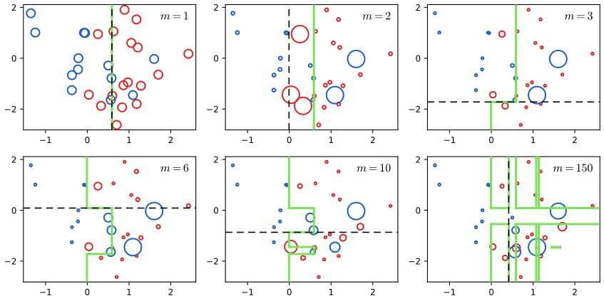
fig14_2. Download: PDF · SVGDecision stumps. Each base learner in Figure 14.2 is a decision stump, a tree with a single split (Section 14.4): \(y(\mathbf{x})\)
14.3.1 Minimizing exponential error
Bishop, Section 14.3.1, pp. 659–661. Boosting was first justified by statistical learning theory, through upper bounds on the generalisation error, but those bounds are too loose to explain how well boosting works in practice. Friedman, Hastie and Tibshirani (2000) gave a much simpler explanation: AdaBoost minimises an exponential error function one term at a time. Consider
\[ E=\sum_{n=1}^{N}\exp\{-t_nf_m(\mathbf{x}_n)\}, \tag{14.20} \]where \(f_m\) is a linear combination of base classifiers,
\[ f_m(\mathbf{x})=\frac12\sum_{l=1}^{m}\alpha_l\,y_l(\mathbf{x}). \tag{14.21} \]The number \(t_nf_m(\mathbf{x}_n)\) is the margin of point \(n\): positive when \(f_m\) classifies the point correctly, and larger the more confidently it does so; \(E\) penalises negative margins exponentially. Instead of minimising \(E\) jointly over all the \(\alpha_l\) and \(y_l\), keep \(y_1,\dots,y_{m-1}\) and \(\alpha_1,\dots,\alpha_{m-1}\) fixed and minimise over \(\alpha_m\) and \(y_m\) only. Separating off the contribution of the newest classifier,
\[ E=\sum_{n=1}^{N}\exp\Big\{-t_nf_{m-1}(\mathbf{x}_n)-\frac12t_n\alpha_my_m(\mathbf{x}_n)\Big\}=\sum_{n=1}^{N}w_n^{(m)}\exp\Big\{-\frac12t_n\alpha_my_m(\mathbf{x}_n)\Big\}, \tag{14.22} \]where \(w_n^{(m)}\)
Minimising over \(y_m\) is therefore minimising (14.15), and minimising over \(\alpha_m\) gives (14.17) with \(\epsilon_m\) defined by (14.16). Having found \(\alpha_m\) and \(y_m\), the weights for the next round are
\[ w_n^{(m+1)}=w_n^{(m)}\exp\Big\{-\frac12t_n\alpha_my_m(\mathbf{x}_n)\Big\}, \tag{14.24} \]and since
\[ t_ny_m(\mathbf{x}_n)=1-2I(y_m(\mathbf{x}_n)\neq t_n), \tag{14.25} \]the update can be written
\[ w_n^{(m+1)}=w_n^{(m)}\exp(-\alpha_m/2)\exp\{\alpha_mI(y_m(\mathbf{x}_n)\neq t_n)\}. \tag{14.26} \]The factor \(\exp(-\alpha_m/2)\) is the same for every \(n\) and can be dropped, which gives (14.18). Finally, new points are classified by the sign of \(f_M\); the factor \(\frac12\) does not change the sign, which gives (14.19). The four boxes below fill in each step.
Filling the gap 14.4: the weights are the current exponential errors p. 660, (14.22)
Why (14.22) holds, what \(w_n^{(m)}\) means, and why it starts at 1 rather than \(1/N\).
Derivation
By (14.21) the sum up to \(m\) is the sum up to \(m-1\) plus its last term, \(f_m=f_{m-1}+\frac12\alpha_my_m\). Hence \(t_nf_m(\mathbf{x}_n)\)
Summing over \(n\) gives (14.22). The weight \(w_n^{(m)}\) is exactly the contribution of point \(n\) to the exponential error (14.20) of the previous ensemble \(f_{m-1}\): it exceeds 1 for points with negative margin (misclassified by \(f_{m-1}\)) and is close to 0 for points classified correctly with a large margin. For the empty ensemble \(f_0\equiv0\) every \(w_n^{(1)}=1\). The book's algorithm starts from \(1/N\) instead; a positive factor common to all the weights changes nothing (gap box 14.7). ∎
Filling the gap 14.5: splitting the error, and why the best \(y_m\) does not depend on \(\alpha_m\) p. 661, (14.23)
The two lines of (14.23), and the argument that minimising \(E\) over \(y_m\) is the same as minimising \(J_m\) for every \(\alpha_m\gt0\), so that the joint minimisation can be done in two separate steps.
Derivation
First line. Both \(y_m(\mathbf{x}_n)\) and \(t_n\) are \(\pm1\), so \(t_ny_m(\mathbf{x}_n)=+1\) if \(n\in\mathcal{T}_m\) and \(-1\) if \(n\in\mathcal{M}_m\). The factor \(\exp\{-\frac12t_n\alpha_my_m(\mathbf{x}_n)\}\) is therefore \(e^{-\alpha_m/2}\) on \(\mathcal{T}_m\) and \(e^{\alpha_m/2}\) on \(\mathcal{M}_m\), and (14.22) splits into two sums.
Second line. Write the sum over \(\mathcal{T}_m\) as the total minus the sum over \(\mathcal{M}_m\),
\[ \sum_{n\in\mathcal{T}_m}w_n^{(m)}=\sum_{n=1}^{N}w_n^{(m)}-\sum_{n=1}^{N}w_n^{(m)}I(y_m(\mathbf{x}_n)\neq t_n), \]substitute, and collect the two terms that multiply \(\sum_nw_n^{(m)}I(\cdot)\).
Minimising over \(y_m\). Let \(W=\sum_nw_n^{(m)}\), and for a candidate classifier \(y\) let \(J(y)\)
For \(\alpha\gt0\) the coefficient \(e^{\alpha/2}-e^{-\alpha/2}\)
Why only \(\alpha\ge0\). Only the product \(\alpha_my_m\) enters \(f_m\). If the family of base classifiers contains \(-y\) whenever it contains \(y\) (true for stumps), the pair \((-\alpha,-y)\) gives the same \(f_m\) as \((\alpha,y)\), so requiring \(\alpha\ge0\) loses nothing. In such a family \(J(-y)=W-J(y)\), so the best classifier has \(J(y_m)\le W/2\), i.e. \(\epsilon_m\le\frac12\) and \(\alpha_m\ge0\) in (14.17). At \(\alpha=0\), \(E=W\) for every \(y\), which is beaten by the minimum found in the next box whenever \(\epsilon_m\lt\frac12\). ∎
Filling the gap 14.6: the optimal coefficient (14.17), and the factor \(\tfrac12\) p. 661, Exercise 14.6
Differentiate (14.23) with respect to \(\alpha_m\), check that the stationary point is the global minimum, and record the minimum value, which the training-error bound (Result 14.5) uses.
Derivation
With \(W\) as above and \(\epsilon=J(y_m)/W\), which is (14.16), the first line of (14.23) reads (the misclassified points carry \(\epsilon W\), the others \((1-\epsilon)W\))
\[ E(\alpha)=W\big\{\epsilon\,e^{\alpha/2}+(1-\epsilon)\,e^{-\alpha/2}\big\},\qquad \frac{\d E}{\d\alpha}=\frac W2\big\{\epsilon\,e^{\alpha/2}-(1-\epsilon)\,e^{-\alpha/2}\big\}. \]Setting the derivative to zero and multiplying by \(2e^{\alpha/2}/W\) gives \(\epsilon e^{\alpha}=1-\epsilon\), i.e. \(e^{\alpha}=(1-\epsilon)/\epsilon\), which is (14.17): \(\alpha_m\)
The factor \(\frac12\) in (14.21) is a convention, chosen so that the minimiser comes out exactly as (14.17). Without it (\(f_m=\sum_l\alpha_ly_l\)) the same computation, with \(\alpha\) in place of \(\alpha/2\), gives \(\alpha_m\)
Filling the gap 14.7: the weight updates (14.24)–(14.26), and why \(\exp(-\alpha_m/2)\) can be dropped p. 661
Each identity in turn, then a proof by induction that the book's weights and the exponential-error weights differ only by a factor common to all points, so that both procedures make identical choices.
Derivation
(14.24). By definition \(w_n^{(m+1)}\)
(14.25). If \(y_m(\mathbf{x}_n)=t_n\), the left side is \(t_n^2=1\) and the indicator is 0, so the right side is also 1. If \(y_m(\mathbf{x}_n)\neq t_n\), then \(y_m(\mathbf{x}_n)=-t_n\), the left side is \(-1\) and the right side is \(1-2=-1\).
(14.26). Substitute (14.25) into (14.24): \(\exp\{-\frac12\alpha_m(1-2I)\}\)
Dropping the common factor. The algorithm uses the weights only through the minimiser of (14.15), which does not change when every weight is multiplied by the same \(c\gt0\), and through the ratio (14.16), which does not change either. Formally, let \(\tilde w_n^{(m)}\) be the weights of Algorithm 14.2 (started at \(1/N\), updated by (14.18)) and \(w_n^{(m)}\)
so the claim holds at \(m+1\) with \(c_{m+1}=c_me^{\alpha_m/2}\). By induction it holds for every \(m\). ∎
Result 14.4 (AdaBoost is forward stagewise minimisation of the exponential error)
Start from \(f_0\equiv0\). For \(m=1,\dots,M\), choose \(\alpha_m\ge0\) and \(y_m\) from a family of classifiers closed under reversal so as to minimise the exponential error (14.20) of \(f_m=f_{m-1}+\frac12\alpha_my_m\), keeping all earlier terms fixed. Then \(y_m\) minimises the weighted error (14.15) with weights proportional to \(\exp\{-t_nf_{m-1}(\mathbf{x}_n)\}\), \(\alpha_m\)
Proof
Gap box 14.4 puts the error in the form (14.22) with weights \(\exp\{-t_nf_{m-1}(\mathbf{x}_n)\}\); gap box 14.5 shows that the best \(y_m\) minimises (14.15) for every \(\alpha\gt0\) and that \(\alpha\ge0\) is no restriction; gap box 14.6 gives the best \(\alpha_m\) as (14.17); gap box 14.7 shows by induction that these weights are proportional to those of Algorithm 14.2 at every round, so the two procedures choose the same \(y_m\) and \(\alpha_m\). Finally \(\operatorname{sign}f_M\)
The procedure is stagewise, not a full minimisation: earlier terms are never refitted, so AdaBoost does not find the global minimum of (14.20) over all coefficients and classifiers; it is a greedy coordinate descent in a space of functions. Note also that \(E\) keeps decreasing after the training error has reached zero, by pushing the margins \(t_nf_m(\mathbf{x}_n)\) further up. This is one explanation of the common observation that the test error of boosting often keeps falling after the training error is zero (Schapire, Freund, Bartlett and Lee, 1998), although with noisy labels boosting does overfit (Section 14.3.2).
Result 14.5 (Going further: the training error falls exponentially fast; Freund and Schapire, 1997)
Let \(\gamma_m=\frac12-\epsilon_m\). The training error of the AdaBoost classifier (14.19), counting a tie \(f_M(\mathbf{x}_n)=0\) as an error, satisfies
\[ \frac{1}{N}\sum_{n=1}^{N}I\big(t_nf_M(\mathbf{x}_n)\le0\big)\le\frac1N\sum_{n=1}^{N}e^{-t_nf_M(\mathbf{x}_n)}=\prod_{m=1}^{M}2\sqrt{\epsilon_m(1-\epsilon_m)}=\prod_{m=1}^{M}\sqrt{1-4\gamma_m^2}\le\exp\Big(-2\sum_{m=1}^{M}\gamma_m^2\Big). \]In particular, if every base classifier beats chance by a fixed amount, \(\epsilon_m\le\frac12-\gamma\) with \(\gamma\gt0\), the training error is at most \(e^{-2M\gamma^2}\), and it is exactly zero as soon as \(M\gt\ln N/(2\gamma^2)\).
Proof
First inequality. \(I(z\le0)\le e^{-z}\) for every real \(z\): if \(z\le0\) the right side is at least 1, and if \(z\gt0\) the left side is 0. Apply it with \(z=t_nf_M(\mathbf{x}_n)\) and average over \(n\).
The product. Let \(E_m\)
The last two steps. \(4\epsilon_m(1-\epsilon_m)\)
This is a statement about the training error only, but it is the precise sense in which boosting turns weak learners into a strong one (Schapire, 1990): any fixed edge \(\gamma\) over random guessing, sustained over the rounds, drives the training error to zero exponentially fast.
14.3.2 Error functions for boosting
Bishop, Section 14.3.2, pp. 661–663. To see what minimising the exponential error achieves, replace the sum over training points by its expectation under the joint distribution of \((\mathbf{x},t)\):
\[ \E_{\mathbf{x},t}\big[\exp\{-ty(\mathbf{x})\}\big]=\sum_{t}\int\exp\{-ty(\mathbf{x})\}\,p(t\given\mathbf{x})\,p(\mathbf{x})\,\d\mathbf{x}. \tag{14.27} \]Minimising over all functions \(y(\mathbf{x})\) gives half the log odds:
\[ y(\mathbf{x})=\frac12\ln\Big\{\frac{p(t=1\given\mathbf{x})}{p(t=-1\given\mathbf{x})}\Big\}. \tag{14.28} \]Filling the gap 14.8: the minimiser of the expected exponential error is half the log odds p. 661, (14.28), Exercise 14.7
The book calls this a variational minimisation. Because (14.27) involves \(y\) only through its value at the same \(\mathbf{x}\) (no derivatives of \(y\), no coupling between different inputs), it can be minimised one \(\mathbf{x}\) at a time.
Derivation
Write \(p_+(\mathbf{x})\)
Pointwise minimisation is enough. If a function \(y^\star\) minimises \(g_{\mathbf{x}}(\cdot)\) at every \(\mathbf{x}\), then any other function \(y\) has \(g_{\mathbf{x}}(y(\mathbf{x}))\)
One variable. For \(0\lt p_+\lt1\), \(g(y)=p_+e^{-y}+(1-p_+)e^{y}\) has \(g'(y)=-p_+e^{-y}+(1-p_+)e^{y}\) and \(g''(y)=p_+e^{-y}+(1-p_+)e^{y}\gt0\). So \(g\) is strictly convex and its unique minimiser solves \(g'(y)=0\), i.e. \(e^{2y}=p_+/(1-p_+)\), which is (14.28). The minimum value is \(2\sqrt{p_+(1-p_+)}\) (substitute \(e^y=\sqrt{p_+/(1-p_+)}\)). If \(p_+(\mathbf{x})=1\) there is no minimiser: \(g(y)=e^{-y}\) decreases to 0 as \(y\to\infty\), in line with log odds \(+\infty\) (and symmetrically for \(p_+=0\)).
The variational route gives the same equation: the functional derivative of (14.27) with respect to \(y(\mathbf{x})\) is
\[ \big\{-p_+(\mathbf{x})\,e^{-y(\mathbf{x})}+\big(1-p_+(\mathbf{x})\big)\,e^{y(\mathbf{x})}\big\}\,p(\mathbf{x}), \]and setting it to zero is \(g'_{\mathbf{x}}(y(\mathbf{x}))=0\).
Inverting (14.28) gives \(p(t=1\given\mathbf{x})\)
AdaBoost therefore looks for the best approximation to half the log odds among the linear combinations of base classifiers, subject to the stagewise strategy. The sign of the log odds is the Bayes-optimal decision, which motivates the sign in (14.19).
Comparison with other error functions. The minimiser of the cross-entropy error (4.90) is the posterior class probability. With the coding \(t\in\{-1,1\}\) used for support vector machines in Section 7.1.2, and \(p(t=1\given y)=\sigma(y)\), we have \(p(t=-1\given y)\)
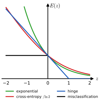
fig14_3. Download: PDF · SVGResult 14.6 (what each classification error estimates)
Fix \(\mathbf{x}\), let \(p=p(t=1\given\mathbf{x})\in(0,1)\), and for an error function \(L\) of the margin let \(y^\star\) minimise the conditional expected error \(pL(y)+(1-p)L(-y)\). Then
- exponential, \(L(z)=e^{-z}\): \(y^\star=\frac12\ln\frac{p}{1-p}\);
- cross-entropy, \(L(z)=\ln(1+e^{-z})\): \(y^\star=\ln\frac{p}{1-p}\);
- hinge, \(L(z)=\max(0,1-z)\): \(y^\star=\operatorname{sign}(2p-1)\) for \(p\neq\frac12\) (any \(y\in[-1,1]\) if \(p=\frac12\));
- misclassification, \(L(z)=I(z\lt0)\): any \(y\) with the sign of \(2p-1\).
All four lead to the Bayes classifier \(\operatorname{sign}(p-\frac12)\); only the first two recover the probability itself, through \(p=\sigma(2y^\star)\) and \(p=\sigma(y^\star)\) respectively.
Proof
Exponential: gap box 14.8. Cross-entropy: \(\frac{\d}{\d y}\ln(1+e^{y})\)
Hinge: for \(|y|\le1\) both hinges are active and \(g(y)=p(1-y)+(1-p)(1+y)\)
Misclassification: the expected error is \(1-p\) if \(y\gt0\) and \(p\) if \(y\lt0\), so the smaller one is obtained by giving \(y\) the sign of \(2p-1\). ∎
Error functions with this property are called classification-calibrated; Bartlett, Jordan and McAuliffe (2006) show that for convex errors it is equivalent to \(L\) being differentiable at 0 with \(L'(0)\lt0\), and that the excess expected error of \(L\) then controls the excess misclassification rate.
Robustness. Where the error functions differ is in their treatment of badly misclassified points, \(z=ty(\mathbf{x})\ll0\): the cross-entropy and hinge errors grow linearly in \(|z|\), the exponential error exponentially. In AdaBoost this is visible in the weights. By gap box 14.4 the weight of point \(n\) is \(w_n=e^{-z_n}\), so a point with margin \(z=-5\) weighs \(e^5\approx148\) times as much as a point on the decision boundary. A mislabelled point, or an outlier deep inside the other class, cannot be classified correctly by any reasonable ensemble; its margin stays negative, its weight keeps growing, and later base classifiers are increasingly spent on it. For the cross-entropy the corresponding weight, the slope \(-\frac{\d}{\d z}\ln(1+e^{-z})\)
Filling the gap 14.9: the exponential error is not a log likelihood p. 662, Exercise 14.8
Unlike the cross-entropy, (14.20) cannot be the negative log likelihood of a correctly normalised model \(p(t\given\mathbf{x})\).
Derivation
Suppose (14.20) were the negative log likelihood of a model for the labels, up to an additive constant \(c\) that does not depend on the model function \(y\): \(-\ln p(t\given\mathbf{x})\)
But \(G\) is not constant: \(G(0)=2/e\approx0.736\), while \(G(y)\to1\) as \(y\to\pm\infty\) (for instance \(G(3)\approx0.951\)). So no constant \(c\) makes \(p(t\given\mathbf{x})\) sum to one for all values of \(y(\mathbf{x})\), and letting \(c\) depend on \(y\) would add the term \(\ln G(y(\mathbf{x}))\) to the error, which is then no longer (14.20). By contrast the cross-entropy error comes from \(p(t\given y)=\sigma(ty)\), and \(\sigma(y)+\sigma(-y)=1\) for every \(y\). ∎
More than two classes. The exponential error does not extend to \(K\gt2\) classes in a natural way. It is built on the scalar margin \(ty(\mathbf{x})\), which needs the coding \(t=\pm1\); with \(K\) classes there is no single sign to flip. One can run \(K\) separate one-against-the-rest problems, but nothing then ties the \(K\) scores together into a probability distribution, whereas the cross-entropy extends directly, through the softmax, to the error (4.108) of a normalised multiclass model (Bishop, Section 4.3.4). A naive multiclass AdaBoost, with \(K\)-class base classifiers in Algorithm 14.2, needs \(\epsilon_m\lt\frac12\) for \(\alpha_m\gt0\), which is much stronger than "better than random guessing" (\(\epsilon_m\lt1-\frac1K\)) when \(K\) is large. The SAMME algorithm of Zhu, Zou, Rosset and Hastie (2009) repairs this with \(\alpha_m\)
Regression. The view of Friedman et al. opens the way to boosting with other error functions, and to regression (Friedman, 2001). With the sum-of-squares error, stagewise minimisation of the additive model (14.21) simply fits each new base learner to the residuals \(t_n-f_{m-1}(\mathbf{x}_n)\) of the previous model.
Filling the gap 14.10: boosting with squared error fits the residuals p. 662, Exercise 14.9
Substitute \(f_m=f_{m-1}+\frac12\alpha_my_m\) into the sum-of-squares error and read off what is being fitted.
Derivation
With \(E\)
where \(r_n\) are the residuals of the previous model. For fixed \(\alpha_m\), minimising over \(y_m\) is a least-squares fit of the function \(\frac12\alpha_my_m\) to the data \(\{(\mathbf{x}_n,r_n)\}\). If the base family is closed under scaling (linear models, regression trees with free leaf values), one simply fits \(y_m\) to the residuals by least squares and absorbs the scale into \(\alpha_m\). For a given \(y_m\), \(\partial E/\partial\alpha_m\)
twice the least-squares coefficient of \(r\) on \(y_m\) (twice because of the \(\frac12\)); \(E\) is a convex quadratic in \(\alpha_m\), so this is the minimum. The method is known as \(L_2\) boosting (Bühlmann and Yu, 2003). For a general differentiable error, Friedman's (2001) gradient boosting fits \(y_m\) to the negative gradient \(-\partial E/\partial f(\mathbf{x}_n)\) at \(f=f_{m-1}\); for the sum-of-squares error that negative gradient is exactly the residual \(r_n\). ∎
The sum-of-squares error is not robust: the pull of a point grows in proportion to its error. The absolute error \(|y-t|\) grows only linearly, with slope \(\pm1\), so it gives much less weight to large errors and to mislabelled points (Figure 14.4); in gradient boosting it amounts to fitting each base learner to the signs of the residuals. The two errors also estimate different things.
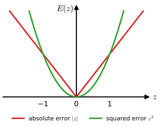
fig14_4. Download: PDF · SVGResult 14.7 (squared error estimates the mean, absolute error the median)
For a random variable \(t\) with finite mean, \(\E[(t-c)^2]\) is minimised by \(c=\E[t]\), and \(\E|t-c|\) by any median of \(t\). Applied conditionally on \(\mathbf{x}\), the minimisers over functions \(y(\mathbf{x})\) are the conditional mean \(\E[t\given\mathbf{x}]\) and the conditional median.
Proof
Adding and subtracting \(\E[t]\), \(\E[(t-c)^2]=\var[t]+(\E[t]-c)^2\) because the cross term has expectation zero; this is smallest at \(c=\E[t]\). For the absolute error, with distribution function \(F\) of a continuous \(t\),
\[ \E|t-c|=\int_{-\infty}^{c}(c-t)\,p(t)\,\d t+\int_{c}^{\infty}(t-c)\,p(t)\,\d t,\qquad \frac{\d}{\d c}\E|t-c|=F(c)-\{1-F(c)\}=2F(c)-1, \]by the Leibniz rule (the boundary terms vanish because the integrands are 0 at \(t=c\)). The derivative is negative below the median and positive above it, so the minimum is where \(F(c)=\frac12\); Exercise 1.27 is the same calculation. For a general distribution the one-sided derivatives at a median \(c\), \(P(t\le c)-P(t\gt c)\ge0\) on the right and \(P(t\lt c)-P(t\ge c)\le0\) on the left, give the same conclusion. Pointwise minimisation, as in gap box 14.8, transfers both results to functions of \(\mathbf{x}\). ∎
A single gross error can move a mean arbitrarily far, but it moves a median by at most one rank: that is the robustness of Figure 14.4 in one sentence.
14.4 Tree-based models
Bishop, Section 14.4, pp. 663–666. Tree-based models cut the input space into axis-aligned boxes and give a simple model, for example a constant, to each region. They are a model combination in which exactly one model is responsible for any given input, and finding that model is a sequence of binary decisions: a walk down a binary tree. The book focuses on CART, classification and regression trees (Breiman, Friedman, Olshen and Stone, 1984); ID3 and C4.5 (Quinlan, 1986, 1993) are close relatives.
Definition 14.2 (a decision tree)
A binary tree \(T\) in which every internal node holds a test "\(x_j\le\theta\)?" on one input variable \(j\) with a threshold \(\theta\), and whose leaves \(\tau=1,\dots,|T|\) correspond to regions \(\mathcal{R}_\tau\): the inputs that arrive at leaf \(\tau\) when the tests are applied from the root down. The regions are disjoint and cover the input space, and the tree predicts
\[ y(\mathbf{x})=\sum_{\tau=1}^{|T|}y_\tau\,I(\mathbf{x}\in\mathcal{R}_\tau), \]a constant \(y_\tau\) in each region (a number for regression; a class label or a vector of class probabilities for classification). In the language of (14.1), the "mixing coefficients" \(\pi_\tau(\mathbf{x})\)
Figures 14.5 and 14.6 show a recursive binary partition and its tree. The first step divides the whole input space according to whether \(x_1\le\theta_1\) or \(x_1\gt\theta_1\); each half can then be divided independently, for instance the region \(x_1\le\theta_1\) by whether \(x_2\le\theta_2\), giving the regions A and B. A new input is classified by starting at the root and following the tests down to a leaf. (Despite the drawing, a decision tree is not a probabilistic graphical model.) Trees are popular in fields such as medical diagnosis because they are easy to read: "is the temperature above some threshold? If so, is the blood pressure below some threshold?", and so on down to a diagnosis at a leaf.
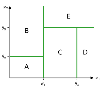
fig14_5. Download: PDF · SVG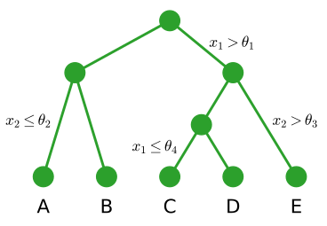
fig14_6. Download: PDF · SVGErratum, p. 663: early printings say "Figure 14.5 shows"; it should be "Figures 14.5 and 14.6 show".
Learning a tree means choosing its structure (which variable and which threshold at each node) and the value in each leaf. Take regression first: predict a scalar \(t\) from \(\mathbf{x}=(x_1,\dots,x_D)^\T\) with training data \(\{\mathbf{x}_n,t_n\}\). If the partition is given and we minimise the sum-of-squares error, the best value in each region is the average of the \(t_n\) that fall in it.
Filling the gap 14.11: the best constant in a region is the mean (or the majority class) p. 664, (14.29), Exercise 14.10
The minimisation decouples over regions; each piece is a one-variable quadratic. For classification, the majority class minimises the error count and the class proportions maximise the likelihood.
Derivation
With the partition fixed, the error is \(\sum_\tau\sum_{\mathbf{x}_n\in\mathcal{R}_\tau}(t_n-y_\tau)^2\), and \(y_\tau\) appears only in the \(\tau\)th inner sum because each point lies in exactly one region. So each \(y_\tau\) is found separately by minimising \(q(c)\)
Classification. In a region with class counts \(N_{\tau k}\) (\(\sum_kN_{\tau k}=N_\tau\)), predicting class \(j\) misclassifies \(N_\tau-N_{\tau j}\) points, which is smallest for the majority class. If the leaf instead predicts class probabilities \(q_1,\dots,q_K\), scored by the log likelihood \(\sum_kN_{\tau k}\ln q_k\), maximise \(\sum_kN_{\tau k}\ln q_k+\lambda(\sum_kq_k-1)\) (Lagrange multiplier): \(N_{\tau k}/q_k+\lambda=0\), so \(q_k=-N_{\tau k}/\lambda\); summing over \(k\) gives \(\lambda=-N_\tau\), hence \(q_k=N_{\tau k}/N_\tau=p_{\tau k}\), the class proportions in the region. The objective is concave in \(\mathbf{q}\), so this stationary point is the maximum. ∎
Growing the tree. Finding the optimal structure, even for a fixed number of leaves, is computationally infeasible because the number of possible trees is combinatorially large. CART grows the tree greedily: start from a single root node (the whole input space) and add nodes one at a time. At each step, every current leaf is a candidate region to split, with a choice of input variable and threshold; for each choice the best leaf values are the local averages, and the split giving the smallest residual sum of squares is kept. The following identity makes this search fast.
Result 14.8 (what one split gains)
Split a region with \(N\) points and mean \(\bar t\) into two parts with \(N_L\) and \(N_R\) points and means \(\bar t_L\), \(\bar t_R\). The residual sum of squares decreases by
\[ Q_{\text{parent}}-Q_L-Q_R=\frac{N_LN_R}{N}\,(\bar t_L-\bar t_R)^2\ \ge0 . \]Proof
For a point on side \(s\in\{L,R\}\), \(t_n-\bar t\)
Since \(\bar t=(N_L\bar t_L+N_R\bar t_R)/N\), we have \(\bar t_L-\bar t\)
So a split never increases the training error, and the best threshold for variable \(j\) is found by sorting the points by \(x_j\) and sweeping through the \(N-1\) gaps with running sums of \(t_n\) (which give the two means), in \(O(N)\) time after sorting. This is the "exhaustive search" of the book.
When to stop. Stopping as soon as the best split reduces the error by less than a threshold does not work well: often no single split helps, yet a few more splits help a lot. A clean example is the "exclusive or": put equal numbers of points at the four corners \((\pm1,\pm1)\) with \(t=x_1x_2\). Any split leaves both sides with equally many targets \(+1\) and \(-1\), hence equal means and, by Result 14.8, no gain at all; but after splitting on \(x_1\), splitting each half on \(x_2\) makes every leaf pure and the error zero. CART therefore grows a large tree \(T_0\), stopping only when leaves contain few data points, and then prunes it back. A subtree \(T\subset T_0\) is obtained by collapsing internal nodes (merging their regions). With leaves \(\tau=1,\dots,|T|\), leaf \(\tau\) holding \(N_\tau\) points in region \(\mathcal{R}_\tau\), the optimal prediction and the residual sum of squares of a leaf are
\[ y_\tau=\frac{1}{N_\tau}\sum_{\mathbf{x}_n\in\mathcal{R}_\tau}t_n, \tag{14.29} \] \[ Q_\tau(T)=\sum_{\mathbf{x}_n\in\mathcal{R}_\tau}\{t_n-y_\tau\}^2, \tag{14.30} \]and the pruning criterion trades the error against the number of leaves:
\[ C(T)=\sum_{\tau=1}^{|T|}Q_\tau(T)+\lambda|T|. \tag{14.31} \]The regularisation parameter \(\lambda\ge0\) is chosen by cross-validation. For a given \(\lambda\), the minimisation over the (exponentially many) subtrees is easy, because the criterion is a sum of independent costs over leaves.
Result 14.9 (optimal pruning for a fixed \(\lambda\), and the weakest link)
For a node \(u\) of \(T_0\) let \(Q(u)\) be the residual sum of squares of its points if \(u\) were a leaf, and define, from the leaves of \(T_0\) upwards,
\[ C^\star(u)=\begin{cases}Q(u)+\lambda, & u \text{ a leaf of } T_0,\\ \min\{Q(u)+\lambda,\ C^\star(u_L)+C^\star(u_R)\}, & u \text{ internal, with children } u_L,u_R.\end{cases} \]Then \(C^\star(\text{root})\)
Proof
For any subtree, \(C(T)\)
Weakest-link pruning (outline). By Result 14.8, applied split by split, \(Q(u)\ge Q(T_u)\), so \(g(u)\ge0\): \(g(u)\) is the error reduction per extra leaf bought by the branch below \(u\). Starting from \(T_0\), repeatedly collapse the internal node with the smallest \(g\) (the weakest link), updating \(g\) for its ancestors. This produces a nested sequence \(T_0\supset T_1\supset\dots\supset\{\text{root}\}\) with increasing thresholds \(\lambda_1\le\lambda_2\le\dots\), and Breiman et al. (1984, Chapter 10) prove that \(T_k\) is the smallest minimiser of \(C(T)\) for every \(\lambda\in[\lambda_k,\lambda_{k+1})\). So one pass of pruning yields the solutions for all values of \(\lambda\) at once, and cross-validation only has to choose among the members of this short sequence.
Algorithm 14.3 (CART for regression: grow, then prune)
- Grow. Start with the whole input space as a single leaf. Repeatedly, over all current leaves with at least \(n_{\min}\) points, all input variables \(j\) and all thresholds between consecutive sorted values of \(x_j\) in the leaf, find the split with the largest reduction of the residual sum of squares (Result 14.8) and perform it. Stop when no leaf can be split. Call the result \(T_0\).
- Prune. Compute the weakest-link sequence \(T_0\supset T_1\supset\dots\) and its thresholds \(\lambda_k\) (Result 14.9); choose \(\lambda\), equivalently \(k\), by cross-validation.
- Predict with the leaf means (14.29) of the chosen subtree.
Classification trees. Growing and pruning work the same way with the sum of squares replaced by a measure of the class impurity of each leaf. With \(p_{\tau k}\) the proportion of the points in \(\mathcal{R}_\tau\) that belong to class \(k\), \(k=1,\dots,K\), the two common choices are the cross-entropy and the Gini index:
\[ Q_\tau(T)=-\sum_{k=1}^{K}p_{\tau k}\ln p_{\tau k}, \tag{14.32} \] \[ Q_\tau(T)=\sum_{k=1}^{K}p_{\tau k}(1-p_{\tau k}). \tag{14.33} \]Errata, p. 666
As printed, (14.32) has no minus sign, which would make the impurity negative; the correct form is the one above. The sentence after (14.33) should read: both measures vanish if \(p_{\tau k}=1\) for one \(k\) (so that \(p_{\tau j}=0\) for all \(j\neq k\)), and both have their maxima at \(p_{\tau k}=1/K\) for all \(k\). (The printed version, "vanish for \(p_{\tau k}=0\) and \(p_{\tau k}=1\), maximum at \(p_{\tau k}=0.5\)", is only right for \(K=2\).)
In the pruning criterion (14.31) each per-point impurity is multiplied by the number of points in the leaf, \(N_\tau Q_\tau(T)\), so that, like (14.30), it is a total over data points (Hastie et al., 2009, Section 9.2); without this weighting a leaf with two points would count as much as a leaf with two thousand. The Gini index has two useful readings: \(\sum_kp_k(1-p_k)=1-\sum_kp_k^2\) is the probability that two points drawn at random (with replacement) from the leaf belong to different classes, and it is the error rate of a rule that labels points at random with the leaf's class proportions.
Result 14.10 (why impurities beat the misclassification rate for growing)
Let \(H(\mathbf{p})=-\sum_kp_k\ln p_k\), \(G(\mathbf{p})=\sum_kp_k(1-p_k)\) and \(R(\mathbf{p})=1-\max_kp_k\) (the misclassification rate of the majority vote), for \(\mathbf{p}\) in the probability simplex.
- \(H\) and \(G\) vanish exactly at pure nodes (one \(p_k=1\)) and are maximal at \(p_k=1/K\) for all \(k\), with maxima \(\ln K\) and \(1-1/K\).
- \(H\) and \(G\) are strictly concave. Hence if a node with \(N\) points and proportions \(\mathbf{p}\) is split into children with \(N_L,N_R\) points and proportions \(\mathbf{p}_L,\mathbf{p}_R\), then \(N\,i(\mathbf{p})\)
\({}\ge N_L\,i(\mathbf{p}_L)+N_R\,i(\mathbf{p}_R)\) for \(i=H,G\), with equality only if \(\mathbf{p}_L=\mathbf{p}_R\): every split that changes the class proportions is rewarded. - \(R\) is concave but piecewise linear: if the same class is a majority class in both children, the split does not change \(N\,R(\mathbf{p})\) at all, however much purer one child becomes.
Proof
(a) Each term \(-p\ln p\) (with \(0\ln0=0\)) and \(p(1-p)\) is non-negative on \([0,1]\) and zero only at \(p\in\{0,1\}\), so \(H=0\) or \(G=0\) forces every \(p_k\in\{0,1\}\), i.e. one \(p_k=1\). For the maxima, \(\KL(\mathbf{p}\|\mathbf{u})\)
(b) \(-p\ln p\) has second derivative \(-1/p\lt0\) and \(p(1-p)\) has \(-2\lt0\); a sum of strictly concave functions of the separate coordinates is strictly concave. The parent's proportions are the weighted average \(\mathbf{p}\)
(c) \(R=\min_k(1-p_k)\) is a minimum of linear functions, hence concave. If class \(k\) is a majority class in both children it is one in the parent too, and on that set \(R(\mathbf{p})=1-p_k\) is linear, so \(N(1-p_k)\)
Worked example
A node with class counts (300, 100) is split into (200, 0) and (100, 100). The misclassification count stays at \(100=0+100\): no gain, although one child is now pure. The Gini criterion \(N_\tau G\) falls from \(400\times0.375=150\) to \(0+200\times0.5=100\), and the entropy criterion \(N_\tau H\) from 224.9 to \(0+200\ln2=138.6\) nats: both reward the pure node. Exercise 14.11 makes the same point with two complete trees that have equal misclassification rates (0.25) but different impurities, which both prefer the tree with a pure leaf.
So the cross-entropy and the Gini index are better guides for growing the tree: they respond to every change in the node probabilities, and, unlike the misclassification rate, they are differentiable, which suits gradient-based optimisation. For pruning, where whole subtrees are compared by the quantity we actually care about, the misclassification rate is generally used.
Limitations (p. 666), which motivate the rest of the chapter:
- Instability. The learned tree is very sensitive to the details of the data: a small change in the training set can produce a very different set of splits (Hastie et al., 2001). Trees have low bias and high variance, which makes them the classic base model for bagging and random forests (Section 14.2), and, as stumps, for boosting (Section 14.3).
- Axis-aligned splits. A boundary at 45 degrees to the axes needs a staircase of many splits where a single oblique split would do. For the diagonal \(x_2=x_1\) in the unit square, cutting the square into \(k\) vertical strips and splitting each strip once at the best height uses \(|T|=2k\) leaves and still misclassifies two small triangles per strip, of total area \(k\cdot\frac{1}{4k^2}\)
\({}=\frac{1}{2|T|}\). - Hard splits. Each input belongs to exactly one leaf, so a regression tree is piecewise constant, with jumps at the split boundaries: a poor model for the smooth functions that regression usually aims at.
Section 14.5 removes the last two restrictions by making the splits soft (probabilistic) and allowing them to depend on all the inputs at once.
14.5 Conditional mixture models
Bishop, Section 14.5, pp. 666–667. Decision trees are held back by hard, axis-aligned splits. Both restrictions can be relaxed, at some cost in interpretability, by letting the splits be soft (probabilistic) and depend on all the input variables at once. If the leaf models are probabilistic too, the result is a fully probabilistic tree, the hierarchical mixture of experts of Section 14.5.3. The same family can be reached from the other side: start from the unconditional mixtures of Chapter 9 and replace each component density by a conditional one. The section climbs this ladder one step at a time.
| Model | Mixing weights | Components | M step |
|---|---|---|---|
| Mixture of linear regressions (14.5.1) | constants \(\pi_k\) | \(\N(t\given\mathbf{w}_k^\T\bm{\phi},\beta^{-1})\) | closed form: weighted least squares |
| Mixture of logistic regressions (14.5.2) | constants \(\pi_k\) | \(\Bern(t\given\sigma(\mathbf{w}_k^\T\bm{\phi}))\) | iterative: weighted IRLS per component |
| Mixture of experts (14.5.3) | softmax \(\pi_k(\mathbf{x})\) | either of the above | as above, plus weighted IRLS for the gate |
| Hierarchical mixture of experts (14.5.3) | nested softmax gates | either of the above | as above, one gate at a time |
14.5.1 Mixtures of linear regression models
Bishop, Section 14.5.1, pp. 667–670. A probabilistic linear regression model can be used as a building block. Take \(K\) linear regression models with their own weight vectors \(\mathbf{w}_k\), a common noise precision \(\beta\) (appropriate in many applications, and the case treated here; separate precisions are discussed below), a single target \(t\) (Exercise 14.12 treats a target vector), basis functions \(\bm{\phi}=\bm{\phi}(\mathbf{x})\) and mixing coefficients \(\pi_k\):
\[ p(t\given\bm{\theta})=\sum_{k=1}^{K}\pi_k\,\N(t\given\mathbf{w}_k^\T\bm{\phi},\beta^{-1}), \tag{14.34} \]with \(\bm{\theta}\)
As for Gaussian mixtures (Section 9.2.2), maximise it with EM: introduce binary latent variables \(\mathbf{z}_n\) with \(z_{nk}\in\{0,1\}\), \(\sum_kz_{nk}=1\), saying which component generated point \(n\) (Figure 14.7). The complete-data log likelihood is
\[ \ln p(\mathbf{t},\mathbf{Z}\given\bm{\theta})=\sum_{n=1}^{N}\sum_{k=1}^{K}z_{nk}\ln\big\{\pi_k\,\N(t_n\given\mathbf{w}_k^\T\bm{\phi}_n,\beta^{-1})\big\}. \tag{14.36} \]E step. With current parameters \(\bm{\theta}^{\text{old}}\), the posterior probabilities, or responsibilities, of the components are
\[ \gamma_{nk}=\E[z_{nk}]=p(k\given\bm{\phi}_n,\bm{\theta}^{\text{old}})=\frac{\pi_k\,\N(t_n\given\mathbf{w}_k^\T\bm{\phi}_n,\beta^{-1})}{\sum_j\pi_j\,\N(t_n\given\mathbf{w}_j^\T\bm{\phi}_n,\beta^{-1})}, \tag{14.37} \]and the expected complete-data log likelihood, the function maximised in the M step, is
\[ Q(\bm{\theta},\bm{\theta}^{\text{old}})=\E_{\mathbf{Z}}[\ln p(\mathbf{t},\mathbf{Z}\given\bm{\theta})]=\sum_{n=1}^{N}\sum_{k=1}^{K}\gamma_{nk}\big\{\ln\pi_k+\ln\N(t_n\given\mathbf{w}_k^\T\bm{\phi}_n,\beta^{-1})\big\}. \]Filling the gap 14.12: the complete-data likelihood (14.36), the responsibilities (14.37) and \(Q\) pp. 667–668, Exercise 14.13
Write the joint distribution of one target and its label, multiply over data points, then use Bayes' theorem and the fact that the posterior over labels factorises over \(n\).
Derivation
(14.36). With 1-of-\(K\) coding, \(p(\mathbf{z}_n)\)
(14.37). By Bayes' theorem, \(p(z_{nk}=1\given t_n,\bm{\phi}_n,\bm{\theta})\) is the ratio of \(p(t_n,z_{nk}=1\given\bm{\phi}_n,\bm{\theta})\) to \(\sum_jp(t_n,z_{nj}=1\given\bm{\phi}_n,\bm{\theta})\), which is (14.37). Since \(z_{nk}\in\{0,1\}\), \(\E[z_{nk}]=p(z_{nk}=1\given\cdot)\). (The book writes the responsibility as \(p(k\given\bm{\phi}_n,\bm{\theta}^{\text{old}})\); it is conditioned on \(t_n\) as well.)
\(Q\). The joint distribution factorises over \(n\), so the posterior \(p(\mathbf{Z}\given\mathbf{t},\bm{\theta}^{\text{old}})\)
M step. Maximise \(Q\) with the \(\gamma_{nk}\) held fixed. Because \(Q\) is a sum of a term in \(\bm{\pi}\) alone and terms in \((\mathbf{w}_k,\beta)\), the pieces can be handled one at a time. For the mixing coefficients, with the constraint \(\sum_k\pi_k=1\),
\[ \pi_k=\frac{1}{N}\sum_{n=1}^{N}\gamma_{nk}, \tag{14.38} \]exactly as for unconditional Gaussian mixtures, eq. (9.22). For the weight vector of component \(k\), substituting the Gaussian density,
\[ Q(\bm{\theta},\bm{\theta}^{\text{old}})=\sum_{n=1}^{N}\gamma_{nk}\Big\{-\frac{\beta}{2}\big(t_n-\mathbf{w}_k^\T\bm{\phi}_n\big)^2\Big\}+\const, \tag{14.39} \]where the constant collects every term that does not involve \(\mathbf{w}_k\), including those of the other components. This is the negative of a sum-of-squares error, eq. (3.12), in which point \(n\) carries the weight \(\beta\gamma_{nk}\), an effective precision. So each component is fitted to the whole data set, with every point weighted by the responsibility that component takes for it: a weighted least-squares problem. Setting the derivative with respect to \(\mathbf{w}_k\) to zero,
\[ 0=\sum_{n=1}^{N}\gamma_{nk}\big(t_n-\mathbf{w}_k^\T\bm{\phi}_n\big)\bm{\phi}_n, \tag{14.40} \] \[ 0=\bm{\Phi}^\T\mathbf{R}_k(\mathbf{t}-\bm{\Phi}\mathbf{w}_k), \tag{14.41} \] \[ \mathbf{w}_k=\big(\bm{\Phi}^\T\mathbf{R}_k\bm{\Phi}\big)^{-1}\bm{\Phi}^\T\mathbf{R}_k\mathbf{t}, \tag{14.42} \]with \(\bm{\Phi}\) the \(N\times M\) design matrix (rows \(\bm{\phi}_n^\T\)) and \(\mathbf{R}_k=\diag(\gamma_{nk})\) an \(N\times N\) diagonal matrix. These are modified normal equations, of the same form as the IRLS equations (4.99) of logistic regression; \(\mathbf{R}_k\) changes after every E step, so they are solved afresh in every M step. Finally, keeping only the terms that depend on \(\beta\),
\[ Q(\bm{\theta},\bm{\theta}^{\text{old}})=\sum_{n=1}^{N}\sum_{k=1}^{K}\gamma_{nk}\Big\{\frac12\ln\beta-\frac{\beta}{2}\big(t_n-\mathbf{w}_k^\T\bm{\phi}_n\big)^2\Big\}, \tag{14.43} \]and setting the derivative with respect to \(\beta\) to zero gives
\[ \frac{1}{\beta}=\frac{1}{N}\sum_{n=1}^{N}\sum_{k=1}^{K}\gamma_{nk}\big(t_n-\mathbf{w}_k^\T\bm{\phi}_n\big)^2. \tag{14.44} \]Filling the gap 14.13: the mixing coefficients (14.38) by a Lagrange multiplier p. 668, Exercise 14.14
Maximise \(\sum_n\sum_k\gamma_{nk}\ln\pi_k\) on the probability simplex.
Derivation
Only the term \(\sum_n\sum_k\gamma_{nk}\ln\pi_k\)
Filling the gap 14.14: the weighted least-squares solution (14.39)–(14.42) pp. 668–669
Expand the log density, differentiate with respect to \(\mathbf{w}_k\), write the result in matrix form, and check that the stationary point is a maximum.
Derivation
(14.39). \(\ln\N(t\given\mathbf{w}_k^\T\bm{\phi},\beta^{-1})\)
(14.40). \(\nabla_{\mathbf{w}}(t-\mathbf{w}^\T\bm{\phi})^2\)
(14.41). The vector \(\sum_n\bm{\phi}_n\,c_n\) is \(\bm{\Phi}^\T\mathbf{c}\), and here \(c_n\)
(14.42). Expanding, \(\bm{\Phi}^\T\mathbf{R}_k\bm{\Phi}\,\mathbf{w}_k\)
Maximum. The Hessian of \(Q\) with respect to \(\mathbf{w}_k\) is \(-\beta\bm{\Phi}^\T\mathbf{R}_k\bm{\Phi}\), and \(\mathbf{u}^\T\bm{\Phi}^\T\mathbf{R}_k\bm{\Phi}\mathbf{u}\)
Filling the gap 14.15: the noise precision (14.43)–(14.44), and the order of the updates p. 669
Differentiate (14.43) with respect to \(\beta\), and see why (14.44) must use the new weight vectors.
Derivation
Keeping the terms of \(Q\) that involve \(\beta\) gives (14.43). Its derivative is \(\sum_n\sum_k\gamma_{nk}\{\frac{1}{2\beta}-\frac12(t_n-\mathbf{w}_k^\T\bm{\phi}_n)^2\}\). Since \(\sum_n\sum_k\gamma_{nk}=N\), setting it to zero gives \(\frac{N}{2\beta}\)
Order of the updates. The M step must maximise \(Q\) jointly over \((\mathbf{W},\beta)\). Because the maximiser (14.42) over \(\mathbf{w}_k\) is the same for every \(\beta\) (gap box 14.14), the joint maximum is reached by first computing the new \(\mathbf{w}_k\) and then evaluating (14.44) at those new values: for any \((\mathbf{W},\beta)\), \(Q(\mathbf{W},\beta)\)
Algorithm 14.4 (EM for a mixture of linear regressions)
- Initialise \(\mathbf{w}_k\), \(\pi_k\) and \(\beta\) (Figure 14.8 starts \(\beta\) at the reciprocal of the variance of the targets).
- E step. Compute the responsibilities \(\gamma_{nk}\) by (14.37).
- M step. Update \(\pi_k\) by (14.38); then each \(\mathbf{w}_k\) by the weighted least-squares solution (14.42); then \(\beta\) by (14.44) using the new \(\mathbf{w}_k\).
- Evaluate the log likelihood (14.35); it never decreases (the general EM argument of Section 9.4). Stop when it changes by less than a tolerance, otherwise return to step 2.
Three remarks for statisticians. (i) The shared precision protects the likelihood from the singularities of Section 9.2.1. With component-specific precisions \(\beta_k\), a component could pass exactly through \(M\) points (\(M\) parameters, \(M\) equations), and letting \(\beta_k\to\infty\) would send the likelihood to infinity while the other components keep the remaining points' densities positive. With a shared \(\beta\), letting \(\beta\to\infty\) drives the density of every point that no line fits exactly to zero, so the likelihood is bounded unless all points lie exactly on \(K\) lines. (ii) Relabelling the components gives the same likelihood, so there are always \(K!\) equivalent maxima; identifiability of mixtures of regressions beyond this label switching needs conditions on the design (Hennig, 2000). (iii) The model goes back to switching regressions in econometrics (Quandt and Ramsey, 1978) and to De Veaux (1989), who studied exactly this EM algorithm.
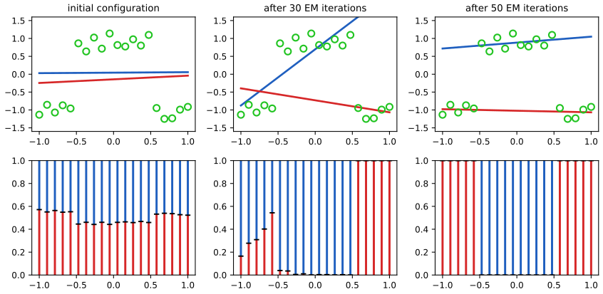
fig14_8. Download: PDF · SVGThe predictive density. Figure 14.9 plots (14.34) at the converged parameters, next to a single linear regression fitted by maximum likelihood. The mixture describes the data much better, and the book reports log likelihoods of \(-3.0\) against \(-27.6\) (our reproduction: \(-3.08\) and \(-27.66\)). But the mixture also puts substantial probability where there are no data, because its predictive density is bimodal at every \(x\). How far apart must the components be for this?
Result 14.11 (when is a two-component mixture bimodal?)
The density \(f(t)\)
Proof
Shift and rescale so that \(\mu_{1,2}=\mp a\) with \(a\ge0\) and \(\sigma=1\); then \(f(t)\propto\varphi(t-a)+\varphi(t+a)\) with \(\varphi\) the standard normal density, and \(f\) is symmetric about 0, so \(f'(0)=0\). Using \(\varphi'(u)=-u\varphi(u)\), a stationary point \(t\gt0\) satisfies \((a-t)\varphi(t-a)\)
Let \(g(t)=a\tanh(at)-t\) for \(t\ge0\): \(g(0)=0\) and \(g'(t)\)
With unequal weights a larger separation is needed (Robertson and Fryer, 1969). Figure 14.9 is the equal-weight case: in our reproduction the converged mixing coefficients are \(\pi=(0.50,0.50)\), the noise standard deviation is \(\beta^{-1/2}=0.14\), and the two lines are 1.91 apart at \(x=0\) (between 1.70 and 2.12 over the range of \(x\)), about 13.5 standard deviations, far beyond the threshold 2 of Result 14.11. So \(p(t\given x)\) has two well-separated modes at every \(x\), including the middle range of \(x\) where the lower line has no data at all. The mixing coefficients cannot switch the lower component off there, because they do not depend on \(x\). Letting them depend on \(x\) is the cure: mixture density networks (Bishop, Section 5.6) and the mixtures of experts of Section 14.5.3. A second symptom of multimodality: the conditional mean, the optimal prediction under squared loss, is (Exercise 14.15)
\[ \E[t\given\mathbf{x}]=\sum_{k=1}^{K}\pi_k\,\mathbf{w}_k^\T\bm{\phi}(\mathbf{x}),\qquad \var[t\given\mathbf{x}]=\beta^{-1}+\sum_{k=1}^{K}\pi_k\big(\mathbf{w}_k^\T\bm{\phi}(\mathbf{x})-\E[t\given\mathbf{x}]\big)^2, \]so in Figure 14.9 the "best" point prediction runs between the two lines, through a region with almost no probability, and the variance is inflated by the spread of the component means.
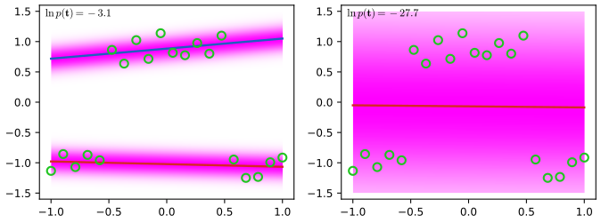
fig14_9. Download: PDF · SVG14.5.2 Mixtures of logistic models
Bishop, Section 14.5.2, pp. 670–672. Logistic regression defines a conditional distribution for a binary target \(t\in\{0,1\}\), so it can serve as a mixture component too. For \(K\) components,
\[ p(t\given\bm{\phi},\bm{\theta})=\sum_{k=1}^{K}\pi_k\,y_k^{t}\,[1-y_k]^{1-t}, \tag{14.45} \]where \(y_k\)
with \(y_{nk}\)
the responsibilities (E step)
\[ \gamma_{nk}=\E[z_{nk}]=p(k\given\bm{\phi}_n,\bm{\theta}^{\text{old}})=\frac{\pi_k\,y_{nk}^{t_n}[1-y_{nk}]^{1-t_n}}{\sum_j\pi_j\,y_{nj}^{t_n}[1-y_{nj}]^{1-t_n}}, \tag{14.48} \]and the expected complete-data log likelihood
\[ Q(\bm{\theta},\bm{\theta}^{\text{old}})=\E_{\mathbf{Z}}[\ln p(\mathbf{t},\mathbf{Z}\given\bm{\theta})]=\sum_{n=1}^{N}\sum_{k=1}^{K}\gamma_{nk}\big\{\ln\pi_k+t_n\ln y_{nk}+(1-t_n)\ln(1-y_{nk})\big\}. \tag{14.49} \]The derivations of (14.47)–(14.49) are word for word those of gap box 14.12 with the Gaussian density replaced by the Bernoulli probability \(y_{nk}^{t_n}[1-y_{nk}]^{1-t_n}\). In the M step the mixing coefficients come out as before (gap box 14.13),
\[ \pi_k=\frac{1}{N}\sum_{n=1}^{N}\gamma_{nk}. \tag{14.50} \]The function \(Q\) is a sum over \(k\) of terms each involving only one \(\mathbf{w}_k\), so the components decouple in the M step: they interact only through the responsibilities, which are fixed there. There is no closed form, but IRLS (Bishop, Section 4.3.3) works, with gradient and Hessian
\[ \nabla_kQ=\sum_{n=1}^{N}\gamma_{nk}(t_n-y_{nk})\bm{\phi}_n, \tag{14.51} \] \[ \mathbf{H}_k=-\nabla_k\nabla_kQ=\sum_{n=1}^{N}\gamma_{nk}\,y_{nk}(1-y_{nk})\,\bm{\phi}_n\bm{\phi}_n^\T, \tag{14.52} \]where \(\nabla_k\) is the gradient with respect to \(\mathbf{w}_k\). Each M step is thus a logistic regression fitted to a weighted data set in which point \(n\) carries weight \(\gamma_{nk}\).
Filling the gap 14.16: the gradient (14.51), the Hessian (14.52), and IRLS with responsibilities p. 672
Differentiate one Bernoulli log likelihood through the sigmoid, check concavity, and write the Newton step as weighted least squares.
Derivation
Gradient. With \(a=\mathbf{w}_k^\T\bm{\phi}_n\) and \(y=\sigma(a)\), \(\frac{\d y}{\d a}=y(1-y)\) (Bishop (4.88)). Then
\[ \frac{\d}{\d a}\big\{t\ln y+(1-t)\ln(1-y)\big\}=\Big\{\frac{t}{y}-\frac{1-t}{1-y}\Big\}y(1-y)=t(1-y)-(1-t)y=t-y, \]and \(\nabla_{\mathbf{w}_k}a=\bm{\phi}_n\). Multiplying by \(\gamma_{nk}\) and summing over \(n\) gives (14.51); the term \(\gamma_{nk}\ln\pi_k\) does not involve \(\mathbf{w}_k\).
Hessian. Differentiating \((t_n-y_{nk})\bm{\phi}_n\) once more gives \(-y_{nk}(1-y_{nk})\bm{\phi}_n\bm{\phi}_n^\T\); with the weights this is \(-\mathbf{H}_k\), so (14.52). For any \(\mathbf{u}\), \(\mathbf{u}^\T\mathbf{H}_k\mathbf{u}\)
IRLS form. Let \(\bm{\Gamma}_k=\diag(\gamma_{nk})\), \(\mathbf{R}=\diag(y_{nk}(1-y_{nk}))\), \(\mathbf{S}_k\)
(factor \(\bm{\Phi}^\T\mathbf{S}_k\) out of \(\bm{\Phi}^\T\mathbf{S}_k\bm{\Phi}\mathbf{w}_k^{\text{old}}+\bm{\Phi}^\T\bm{\Gamma}_k(\mathbf{t}-\mathbf{y}_k)\), using \(\mathbf{S}_k^{-1}\bm{\Gamma}_k\)
Algorithm 14.5 (EM for a mixture of logistic regressions)
- Initialise \(\pi_k\) and \(\mathbf{w}_k\) (different for different \(k\), or the components stay identical).
- E step. Responsibilities (14.48).
- M step. \(\pi_k\) by (14.50); for each \(k\), run IRLS with weights \(\gamma_{nk}y_{nk}(1-y_{nk})\) and working response \(\mathbf{z}_k\) (gap box 14.16) until \(\mathbf{w}_k\) settles, or for a few steps that increase \(Q\).
- Evaluate the log likelihood \(\ln p(\mathbf{t}\given\bm{\theta})\) from (14.46) and repeat until it stops changing.
What the mixture adds. For a binary target the mixture (14.45) is again a Bernoulli distribution: \(p(t=1\given\bm{\phi})\)
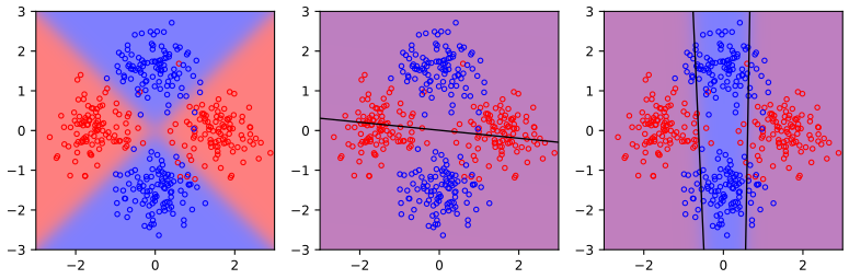
fig14_10. Download: PDF · SVG14.5.3 Mixtures of experts
Bishop, Section 14.5.3, pp. 672–674. The mixtures of 14.5.1 and 14.5.2 extend linear models to multimodal predictive distributions, but they remain limited, as Figure 14.9 shows. The next step lets the mixing coefficients depend on the input:
\[ p(\mathbf{t}\given\mathbf{x})=\sum_{k=1}^{K}\pi_k(\mathbf{x})\,p_k(\mathbf{t}\given\mathbf{x}). \tag{14.53} \]Definition 14.3 (mixture of experts; Jacobs, Jordan, Nowlan and Hinton, 1991)
A model of the form (14.53) in which the component densities \(p_k(\mathbf{t}\given\mathbf{x})\), the experts, are weighted by gating functions \(\pi_k(\mathbf{x})\) with \(0\le\pi_k(\mathbf{x})\le1\) and \(\sum_k\pi_k(\mathbf{x})=1\) for every \(\mathbf{x}\). Each expert models the data in its own region of input space, and the gate decides which experts dominate where. The standard choice of gate is a linear softmax model, Bishop (4.104)–(4.105),
\[ \pi_k(\mathbf{x})=\frac{\exp(\mathbf{v}_k^\T\mathbf{x})}{\sum_{j=1}^{K}\exp(\mathbf{v}_j^\T\mathbf{x})}, \]where \(\mathbf{x}\) includes a constant component 1 for the bias. Adding the same vector to every \(\mathbf{v}_k\) leaves all \(\pi_k(\mathbf{x})\) unchanged, so one fixes \(\mathbf{v}_K=\mathbf{0}\) (or uses a prior); for \(K=2\) the gate is the logistic sigmoid \(\pi_1(\mathbf{x})\)
If the experts are also linear (regression or classification) models, the whole model can be fitted by EM with iterative reweighted least squares in the M step (Jordan and Jacobs, 1994). Bishop states this in one sentence; here is the algorithm in full.
Filling the gap 14.17: EM for a mixture of experts, with IRLS for the gate p. 673
The E step uses the gate as an input-dependent prior; the M step splits into \(K\) weighted expert fits and one softmax regression with "soft" targets, whose gradient and Hessian are derived below.
Derivation
Complete data. As in gap box 14.12, with \(z_{nk}\) the indicator that expert \(k\) produced \(\mathbf{t}_n\), and \(p(z_{nk}=1\given\mathbf{x}_n)\)
E step. By Bayes' theorem,
\[ \gamma_{nk}=\frac{\pi_k(\mathbf{x}_n)\,p_k(\mathbf{t}_n\given\mathbf{x}_n)}{\sum_j\pi_j(\mathbf{x}_n)\,p_j(\mathbf{t}_n\given\mathbf{x}_n)} . \]The gate value \(\pi_k(\mathbf{x}_n)\) is the probability of expert \(k\) before seeing \(\mathbf{t}_n\); the responsibility is the probability after seeing it.
The \(Q\) function separates. Replacing \(z_{nk}\) by \(\gamma_{nk}\),
\[ Q=\underbrace{\sum_{n=1}^{N}\sum_{k=1}^{K}\gamma_{nk}\ln\pi_k(\mathbf{x}_n)}_{L(\mathbf{V}):\ \text{gate only}}+\sum_{k=1}^{K}\underbrace{\sum_{n=1}^{N}\gamma_{nk}\ln p_k(\mathbf{t}_n\given\mathbf{x}_n,\bm{\theta}_k)}_{\text{expert }k\text{ only}} . \]Experts. Each is a weighted fit, exactly as in 14.5.1 or 14.5.2. For linear-Gaussian experts \(\N(t\given\mathbf{w}_k^\T\bm{\phi}(\mathbf{x}),\beta_k^{-1})\) with their own precisions, \(\mathbf{w}_k\) is given by (14.42), and the derivative of \(\sum_n\gamma_{nk}\{\frac12\ln\beta_k-\frac{\beta_k}{2}(t_n-\mathbf{w}_k^\T\bm{\phi}_n)^2\}\) gives \(\beta_k^{-1}\)
Gate. \(L(\mathbf{V})\) is the log likelihood of a softmax regression in which the 1-of-\(K\) target of point \(n\) is replaced by the probability vector \((\gamma_{n1},\dots,\gamma_{nK})\). With \(a_{nj}=\mathbf{v}_j^\T\mathbf{x}_n\) and \(\pi_{nk}=\pi_k(\mathbf{x}_n)\), \(\ln\pi_{nk}\)
using \(\partial a_{nj}/\partial\mathbf{v}_j\)
the multiclass logistic-regression Hessian (4.110) with the sign of a log likelihood. These are the formulas of Bishop (4.109)–(4.110) with the targets \(t_{nj}\) replaced by \(\gamma_{nj}\). Newton's method (IRLS) on \(L\), with \(\mathbf{v}_K=\mathbf{0}\) fixed, completes the M step; Result 14.12 shows that \(L\) is concave. (Both formulas were checked against finite differences.) ∎
Result 14.12 (each M step of a mixture of experts is a concave problem)
The gating objective \(L(\mathbf{V})\)
Proof
For a direction \(\mathbf{u}\)
The brace is the variance of a random variable that takes the value \(s_{nj}\) with probability \(\pi_{nj}\), so it is non-negative and the Hessian is negative semidefinite: \(L\) is concave. Since every \(\pi_{nj}\gt0\), the variance is zero only if \(s_{n1}=\dots=s_{nK}\) for every \(n\), i.e. \((\mathbf{u}_j-\mathbf{u}_l)^\T\mathbf{x}_n\)
Algorithm 14.6 (EM for a mixture of linear-Gaussian experts with a softmax gate; Jordan and Jacobs, 1994)
- Initialise the experts \((\mathbf{w}_k,\beta_k)\) and the gate \(\mathbf{v}_1,\dots,\mathbf{v}_{K-1}\) (\(\mathbf{v}_K=\mathbf{0}\)).
- E step. \(\gamma_{nk}\propto\pi_k(\mathbf{x}_n)\,\N(t_n\given\mathbf{w}_k^\T\bm{\phi}_n,\beta_k^{-1})\), normalised over \(k\).
- M step, experts. \(\mathbf{w}_k\) by (14.42) with \(\mathbf{R}_k=\diag(\gamma_{nk})\); then \(\beta_k^{-1}\)
\({}=\sum_n\gamma_{nk}(t_n-\mathbf{w}_k^\T\bm{\phi}_n)^2/\sum_n\gamma_{nk}\). - M step, gate. Newton (IRLS) steps on \(L(\mathbf{V})\) with the gradient and Hessian of gap box 14.17, halving the step if \(L\) decreases; to convergence for exact EM, or a few steps for generalised EM.
- Evaluate \(\sum_n\ln\sum_k\pi_k(\mathbf{x}_n)\N(t_n\given\mathbf{w}_k^\T\bm{\phi}_n,\beta_k^{-1})\); repeat until it stops changing.
Separate precisions \(\beta_k\) bring back the singularities discussed after Algorithm 14.4 (an expert can fit a few points exactly and let its variance shrink to zero), so in practice one bounds them below or puts a prior on them. Jordan and Xu (1995) analyse the convergence of this EM algorithm.
One limitation of the linear gate is worth seeing concretely. With a scalar input and gating vector \(\mathbf{x}=(1,x)^\T\), a two-expert gate \(\pi_1(x)=\sigma(v_0+v_1x)\) is monotone in \(x\): it can hand one end of the input range to one expert and the other end to the other, but it cannot switch an expert off only in the middle. For data like those of Figure 14.9, where the lower line has data at both ends but not in the middle, the gate needs richer inputs, such as \((1,x,x^2)\), or a second level of gating (the hierarchy below).
Hierarchical mixtures of experts. Linear gates and linear experts are still limiting. A much more flexible model uses a multilevel gate: the hierarchical mixture of experts, or HME (Jordan and Jacobs, 1994), a mixture in which each component is itself a mixture of experts. With constant mixing coefficients a hierarchy of mixtures is just one flat mixture, and even with arbitrary input-dependent coefficients it can be flattened; but with linear softmax gates the hierarchy is genuinely richer (Exercise 14.17). The HME is a probabilistic, soft version of a decision tree: a logistic gate \(\sigma\big(c(x_j-\theta)\big)\) tends to the hard split \(I(x_j\gt\theta)\) as \(c\to\infty\), so CART with constant leaves is a limiting case, while a general gate \(\sigma(\mathbf{v}^\T\mathbf{x})\) splits softly along any direction. It can again be trained by maximum likelihood with EM and IRLS in the M step (below), and Bishop and Svensén (2003) give a Bayesian treatment by variational inference.
Filling the gap 14.18: EM for a two-level HME p. 673
The book says the HME "can again be trained efficiently by maximum likelihood using an EM algorithm with IRLS in the M step" without details. Nested latent variables give path responsibilities, and the M step splits into one weighted problem per gate and per expert.
Derivation
Model. \(p(\mathbf{t}\given\mathbf{x})\)
Latent variables. \(z_i\) picks the branch at the top and \(z_{j|i}\) the expert within branch \(i\); the path indicator \(z_{ij}=z_iz_{j|i}\) equals 1 for exactly one pair. The complete-data log likelihood is
\[ \sum_{n=1}^{N}\sum_{i,j}z_{ij}^{(n)}\big\{\ln g_i(\mathbf{x}_n)+\ln g_{j|i}(\mathbf{x}_n)+\ln p_{ij}(\mathbf{t}_n\given\mathbf{x}_n)\big\}. \]E step. The posterior of a path, and of a top branch, are
\[ h_{ij}^{(n)}=\frac{g_i(\mathbf{x}_n)\,g_{j|i}(\mathbf{x}_n)\,p_{ij}(\mathbf{t}_n\given\mathbf{x}_n)}{\sum_{i'}\sum_{j'}g_{i'}(\mathbf{x}_n)\,g_{j'|i'}(\mathbf{x}_n)\,p_{i'j'}(\mathbf{t}_n\given\mathbf{x}_n)},\qquad h_i^{(n)}=\sum_jh_{ij}^{(n)},\qquad h_{j|i}^{(n)}=\frac{h_{ij}^{(n)}}{h_i^{(n)}} . \]\(Q\) separates. Replace \(z_{ij}^{(n)}\) by \(h_{ij}^{(n)}\) and use \(\sum_jh_{ij}^{(n)}\ln g_i\)
M step. Three kinds of decoupled problems: the top gate is a softmax regression with soft targets \(h_i^{(n)}\); lower gate \(i\) is a softmax regression with soft targets \(h_{j|i}^{(n)}\) in which point \(n\) carries the weight \(h_i^{(n)}\), so its gradient is \(\sum_nh_i^{(n)}(h_{j|i}^{(n)}-g_{j|i}(\mathbf{x}_n))\mathbf{x}_n\); expert \((i,j)\) is fitted with weights \(h_{ij}^{(n)}\). Each is concave, by Result 14.12 and gap boxes 14.14 and 14.16, and is solved by IRLS. ∎
Mixture density networks (Bishop, Section 5.6) are the other way of making the mixing coefficients depend on \(\mathbf{x}\). There, \(\pi_k(\mathbf{x})\), \(\bm{\mu}_k(\mathbf{x})\) and \(\sigma_k^2(\mathbf{x})\) are all outputs of a single neural network trained by gradient descent on the negative log likelihood. The trade-off, as the book puts it: the mixture of experts can be optimised by EM with a convex problem in every M step, although the overall problem is not convex; the mixture density network shares hidden units between the components and the gate, and its splits of input space are not only soft and oblique but can be nonlinear. The two are closer than they look. In Bishop's (5.155), the derivative of the network error with respect to the activation of mixing coefficient \(k\) is \(\pi_k-\gamma_{nk}\), with \(\gamma_{nk}\) the responsibility (5.154): exactly the negative of the gating gradient of gap box 14.17. This is no coincidence.
Result 14.13 (Going further: Fisher's identity links EM and gradient training)
For any latent-variable model, the gradient of the log likelihood at the current parameters equals the gradient of the EM function \(Q\) there:
\[ \nabla_{\bm{\theta}}\ln p(\mathbf{t}\given\bm{\theta})\Big|_{\bm{\theta}=\bm{\theta}^{\text{old}}}=\nabla_{\bm{\theta}}Q(\bm{\theta},\bm{\theta}^{\text{old}})\Big|_{\bm{\theta}=\bm{\theta}^{\text{old}}} . \]For a mixture of experts the gradient with respect to the gate is therefore \(\sum_n(\gamma_{nk}-\pi_k(\mathbf{x}_n))\mathbf{x}_n\), computed with the responsibilities of the current parameters: EM and gradient methods use the same responsibilities; EM takes a full (concave) M step, gradient methods take a small step.
Proof
For every \(\mathbf{Z}\), \(\ln p(\mathbf{t}\given\bm{\theta})\)
The gradient of the last sum at \(\bm{\theta}\)
Going further: mixtures of experts beyond the book
- How flexible are they? With enough experts, softmax-gated mixtures of experts can approximate very general regression functions and conditional densities: Jiang and Tanner (1999) give approximation rates and consistency of maximum likelihood for HMEs in exponential-family regression; Nguyen, Lloyd-Jones and McLachlan (2016) prove a universal approximation theorem for the mean function; Nguyen, Nguyen, Chamroukhi and McLachlan (2021) approximate conditional densities in Lebesgue spaces. Interactive demo: universal approximation for mixtures of experts.
- How well are the parameters estimated? When more experts are fitted than needed, the softmax gate and the experts interact, and maximum likelihood estimates of the parameters converge more slowly than the usual \(N^{-1/2}\), at rates that depend on the gating function (Nguyen, Nguyen and Ho, 2023). Interactive demo: convergence rates in mixtures of experts.
- How many experts? Penalised likelihood with non-asymptotic guarantees selects the number of experts, even in high dimensions (Nguyen, Nguyen, Chamroukhi and Forbes, 2022). Interactive demo: model selection for mixtures of experts.
- Deep learning. Sparse mixture-of-experts layers send each input to the few experts with the largest gate values, so that very large networks use only a fraction of their parameters for any one input (Shazeer et al., 2017). Interactive demos: HyperRouter and CompeteSMoE.
- Surveys: Yuksel, Wilson and Gader (2012); Nguyen and Chamroukhi (2018).
Exercises
All seventeen exercises of the chapter (Bishop, pp. 674–676), restated in my words, with full solutions (hidden). Exercises marked www have official solutions (Svensén and Bishop, 2009); the solutions below are written independently and note the two places where the official ones are inaccurate (Exercises 14.1 and 14.15). Stars give the book's difficulty rating. Several exercises complete derivations in the text; their solutions are self-contained but link to the corresponding gap box.
Exercise 14.1 (★★, www). Consider models \(p(\mathbf{t}\given\mathbf{x},\mathbf{z}_h,\bm{\theta}_h,h)\), \(h=1,\dots,H\), each with a latent variable \(\mathbf{z}_h\), parameters \(\bm{\theta}_h\) and prior probability \(p(h)\), and a training set \(\mathbf{X}=\{\mathbf{x}_n\}\), \(\mathbf{T}=\{\mathbf{t}_n\}\). Write down the formulae for the predictive distribution \(p(\mathbf{t}\given\mathbf{x},\mathbf{X},\mathbf{T})\) with the latent variables and the model index marginalised out, and use them to explain the difference between Bayesian model averaging and latent variables within one model.
Solution
Assume a prior \(p(\bm{\theta}_h\given h)\) for each model, and that given \(h\) and \(\bm{\theta}_h\) the training pairs and the new pair are independent, each target with its own latent variable. Conditioning on the inputs throughout (they carry no information about the parameters of a conditional model),
\[ p(\mathbf{t}\given\mathbf{x},\mathbf{X},\mathbf{T})=\sum_{h=1}^{H}p(h\given\mathbf{X},\mathbf{T})\int p(\mathbf{t}\given\mathbf{x},\bm{\theta}_h,h)\,p(\bm{\theta}_h\given\mathbf{X},\mathbf{T},h)\,\d\bm{\theta}_h, \] \[ p(\mathbf{t}\given\mathbf{x},\bm{\theta}_h,h)=\sum_{\mathbf{z}_h}p(\mathbf{t}\given\mathbf{x},\mathbf{z}_h,\bm{\theta}_h,h)\,p(\mathbf{z}_h\given\mathbf{x},\bm{\theta}_h,h), \] \[ p(\bm{\theta}_h\given\mathbf{X},\mathbf{T},h)=\frac{p(\bm{\theta}_h\given h)}{p(\mathbf{T}\given\mathbf{X},h)}\prod_{n=1}^{N}\Big[\sum_{\mathbf{z}_{nh}}p(\mathbf{t}_n,\mathbf{z}_{nh}\given\mathbf{x}_n,\bm{\theta}_h,h)\Big], \] \[ p(\mathbf{T}\given\mathbf{X},h)=\int p(\bm{\theta}_h\given h)\prod_{n=1}^{N}\Big[\sum_{\mathbf{z}_{nh}}p(\mathbf{t}_n,\mathbf{z}_{nh}\given\mathbf{x}_n,\bm{\theta}_h,h)\Big]\d\bm{\theta}_h,\qquad p(h\given\mathbf{X},\mathbf{T})=\frac{p(h)\,p(\mathbf{T}\given\mathbf{X},h)}{\sum_{h'}p(h')\,p(\mathbf{T}\given\mathbf{X},h')} . \]The first line is the sum and product rules (marginalise \(h\) and \(\bm{\theta}_h\)), the second marginalises the latent variable of the new point, and the last two are Bayes' theorem for \(\bm{\theta}_h\) and for \(h\).
The difference. The latent variables \(\mathbf{z}_{nh}\) are summed inside the product over \(n\): every data point has its own latent state, so within one model different points can be explained by different states (model combination, as in (14.5)). The model index \(h\) is summed outside the product: one \(h\) for the whole data set, and the weights \(p(h\given\mathbf{X},\mathbf{T})\) only express our uncertainty about which model generated all the data. These weights concentrate on a single model as \(N\) grows (Result 14.1), whereas the new point still gets a fresh latent variable with its own distribution \(p(\mathbf{z}_h\given\mathbf{x},\bm{\theta}_h,h)\). (The official solution writes the prior \(p(h)\) where the posterior \(p(h\given\mathbf{X},\mathbf{T})\) is needed.)
Exercise 14.2 (★). Assuming (14.12) and (14.13), derive \(E_{\mathrm{COM}}=E_{\mathrm{AV}}/M\), eq. (14.14), from (14.10) and (14.11).
Solution
\(E_{\mathrm{COM}}\)
\({}\) \({}=\frac{1}{M^2}\sum_m\sum_l\E_{\mathbf{x}}[\epsilon_m\epsilon_l]\). The \(M\) diagonal terms give \(\sum_m\E_{\mathbf{x}}[\epsilon_m^2]\) \({}=ME_{\mathrm{AV}}\) by (14.10), and the off-diagonal terms vanish by (14.13), so \(E_{\mathrm{COM}}\) \({}=ME_{\mathrm{AV}}/M^2\) \({}=E_{\mathrm{AV}}/M\). Only (14.13) is used; see gap box 14.2, and Result 14.2(a) for the general case with correlated errors. Exercise 14.3 (★, www). Use Jensen's inequality (1.115) with the convex function \(f(x)=x^2\) to show that
\[ E_{\mathrm{COM}}\le E_{\mathrm{AV}}. \tag{14.54} \]Solution
Jensen's inequality (toolkit) for a convex \(f\) and weights \(\lambda_m\ge0\) summing to one reads \(f(\sum_m\lambda_mx_m)\)
\({}\le\sum_m\lambda_mf(x_m)\). Take \(\lambda_m=1/M\), \(x_m=\epsilon_m(\mathbf{x})\) and \(f(x)=x^2\): at every \(\mathbf{x}\), \(\big(\frac1M\sum_m\epsilon_m(\mathbf{x})\big)^2\) \({}\le\frac1M\sum_m\epsilon_m(\mathbf{x})^2\). Taking \(\E_{\mathbf{x}}\) of both sides (expectation preserves inequalities) and moving \(\frac1M\sum_m\) outside the expectation on the right gives (14.54). Result 14.2(b) gives the size of the gap: \(E_{\mathrm{AV}}-E_{\mathrm{COM}}\) is the expected spread of the members' errors around their mean. Exercise 14.4 (★★). Show that (14.54) holds for any error function \(E(y)\) that is a convex function of \(y\), not only for the sum of squares.
Solution
Let the error of a prediction \(y\) at input \(\mathbf{x}\) be \(E(y;\mathbf{x})\), convex in \(y\) for each \(\mathbf{x}\) (for instance \(E=|y-h(\mathbf{x})|\), or any convex loss of the residual). Define \(E_{\mathrm{AV}}\)
\({}=\frac1M\sum_m\E_{\mathbf{x}}[E(y_m(\mathbf{x});\mathbf{x})]\) and \(E_{\mathrm{COM}}\) \({}=\E_{\mathbf{x}}[E(y_{\mathrm{COM}}(\mathbf{x});\mathbf{x})]\). Jensen's inequality at each \(\mathbf{x}\), with weights \(1/M\), gives \(E\big(\frac1M\sum_my_m(\mathbf{x});\mathbf{x}\big)\) \({}\le\frac1M\sum_mE(y_m(\mathbf{x});\mathbf{x})\); take \(\E_{\mathbf{x}}\). The same argument works for any committee weights \(\alpha_m\ge0\) with \(\sum_m\alpha_m=1\). Convexity matters. For a majority vote of classifiers scored by the (non-convex) misclassification error, the committee can be worse than its members: take three classifiers and three disjoint regions of input space with probability 0.1 each, such that on each region a different pair of classifiers is wrong, and all are right elsewhere. Each classifier errs with probability 0.2, but the majority errs on all three regions, with probability 0.3.
Exercise 14.5 (★★, www). For a committee with unequal weights,
\[ y_{\mathrm{COM}}(\mathbf{x})=\sum_{m=1}^{M}\alpha_m\,y_m(\mathbf{x}), \tag{14.55} \]require the prediction to stay between the smallest and largest member predictions at every \(\mathbf{x}\),
\[ y_{\min}(\mathbf{x})\le y_{\mathrm{COM}}(\mathbf{x})\le y_{\max}(\mathbf{x}). \tag{14.56} \]Show that a necessary and sufficient condition for (14.56) to hold, whatever the members' predictions, is
\[ \alpha_m\ge0,\qquad \sum_{m=1}^{M}\alpha_m=1. \tag{14.57} \]Solution
Sufficient. If (14.57) holds, \(y_{\mathrm{COM}}(\mathbf{x})\) is a convex combination of the numbers \(y_m(\mathbf{x})\), all of which lie in \([y_{\min}(\mathbf{x}),y_{\max}(\mathbf{x})]\): \(y_{\mathrm{COM}}\)
\({}\) \({}=\sum_m\alpha_my_m\) \({}\ge\sum_m\alpha_my_{\min}\) \({}=y_{\min}\), and likewise \(y_{\mathrm{COM}}\le y_{\max}\). Necessary. Suppose (14.56) holds for every possible set of member predictions. (i) Take \(y_k(\mathbf{x})=1\) and \(y_m(\mathbf{x})=0\) for \(m\neq k\) (\(M\ge2\)): then \(y_{\min}=0\), \(y_{\max}=1\) and \(y_{\mathrm{COM}}=\alpha_k\), so \(0\le\alpha_k\le1\); this holds for every \(k\). (ii) Take all \(y_m(\mathbf{x})=1\): then \(y_{\min}=y_{\max}=1\) and \(y_{\mathrm{COM}}=\sum_m\alpha_m\), so \(\sum_m\alpha_m=1\). (For \(M=1\), (ii) alone gives \(\alpha_1=1\).) This is shorter than the official solution's argument through the smallest coefficient, and it shows what "necessary" means here: the condition must hold for all possible member outputs.
Exercise 14.6 (★, www). By differentiating the error function (14.23) with respect to \(\alpha_m\), show that \(\alpha_m\) is given by (14.17) with \(\epsilon_m\) defined by (14.16).
Solution
Write \(W=\sum_nw_n^{(m)}\) and \(J\)
\[ \frac{\partial E}{\partial\alpha_m}=\frac12\big(e^{\alpha_m/2}+e^{-\alpha_m/2}\big)J-\frac12e^{-\alpha_m/2}W=0\iff\epsilon_m\big(e^{\alpha_m}+1\big)=1\iff e^{\alpha_m}=\frac{1-\epsilon_m}{\epsilon_m}, \]\({}=\sum_nw_n^{(m)}I(y_m(\mathbf{x}_n)\neq t_n)\) \({}=\epsilon_mW\). Differentiating the second line of (14.23), (multiply by \(2e^{\alpha_m/2}/W\) for the middle step), which is (14.17). The second derivative \(\frac14(e^{\alpha_m/2}-e^{-\alpha_m/2})J+\frac14e^{-\alpha_m/2}W\)
\({}=\frac W4\{\epsilon_me^{\alpha_m/2}+(1-\epsilon_m)e^{-\alpha_m/2}\}\) is positive, so this is the minimum. See gap box 14.6, which also gives the minimum value \(2W\sqrt{\epsilon_m(1-\epsilon_m)}\). Exercise 14.7 (★). By minimising the expected exponential error (14.27) over all functions \(y(\mathbf{x})\), show that the minimiser is (14.28).
Solution
Summing over \(t\) inside (14.27), the expected error is \(\int g_{\mathbf{x}}(y(\mathbf{x}))\,p(\mathbf{x})\,\d\mathbf{x}\) with \(g_{\mathbf{x}}(y)\)
\({}=p_+e^{-y}+(1-p_+)e^{y}\) and \(p_+=p(t=1\given\mathbf{x})\). The integrand depends on \(y\) only through \(y(\mathbf{x})\), so it suffices to minimise \(g_{\mathbf{x}}\) at each \(\mathbf{x}\); the functional derivative gives the same condition. \(g'(y)=-p_+e^{-y}+(1-p_+)e^y=0\) gives \(e^{2y}=p_+/(1-p_+)\), i.e. \(y\) \({}=\frac12\ln\{p(t=1\given\mathbf{x})/p(t=-1\given\mathbf{x})\}\), and \(g''\gt0\) shows it is the unique minimum. Details, including the cases \(p_+\in\{0,1\}\): gap box 14.8. Exercise 14.8 (★). Show that the exponential error (14.20) is not the negative log likelihood of any well-behaved probabilistic model, by showing that the corresponding \(p(t\given\mathbf{x})\) cannot be normalised.
Solution
If \(-\ln p(t\given\mathbf{x})\)
\({}=e^{-ty(\mathbf{x})}+c\) with \(c\) not depending on \(y\), then \(p(t=1\given\mathbf{x})+p(t=-1\given\mathbf{x})\) \({}=e^{-c}G(y(\mathbf{x}))\) with \(G(y)=\exp(-e^{-y})+\exp(-e^{y})\). For this to equal 1 for every \(\mathbf{x}\), \(G\) would have to be constant over the values taken by \(y(\mathbf{x})\); but \(G(0)=2/e\approx0.736\) and \(G(y)\to1\) as \(|y|\to\infty\). So no constant normalises the model for all \(y\) (gap box 14.9). By contrast \(p(t\given y)=\sigma(ty)\) is normalised for every \(y\). Exercise 14.9 (★, www). Show that stagewise minimisation of the sum-of-squares error for an additive model of the form (14.21) fits each new base learner to the residuals \(t_n-f_{m-1}(\mathbf{x}_n)\) of the previous model.
Solution
With \(f_m=f_{m-1}+\frac12\alpha_my_m\), \(E\)
\({}=\frac12\sum_n\{t_n-f_m(\mathbf{x}_n)\}^2\) \({}=\frac12\sum_n\{r_n-\frac12\alpha_my_m(\mathbf{x}_n)\}^2\) with residuals \(r_n=t_n-f_{m-1}(\mathbf{x}_n)\). Minimising over \(y_m\) (with \(\alpha_m\) fixed, or absorbed into \(y_m\) if the base family is closed under scaling) is a least-squares fit of \(\frac12\alpha_my_m\) to the data \(\{(\mathbf{x}_n,r_n)\}\). For a given \(y_m\), the optimal coefficient is \(\alpha_m\) \({}=2\sum_nr_ny_m(\mathbf{x}_n)/\sum_ny_m(\mathbf{x}_n)^2\). See gap box 14.10 for the link with gradient boosting. Exercise 14.10 (★). Show that the single value \(c\) minimising the sum-of-squares error \(\sum_n(t_n-c)^2\) is the mean of the \(t_n\).
Solution
\(\frac{\d}{\d c}\sum_n(t_n-c)^2\)
\({}=-2\sum_n(t_n-c)\) \({}=-2(N\bar t-Nc)\), which vanishes at \(c=\bar t\); the second derivative \(2N\) is positive. Without calculus: \(\sum_n(t_n-c)^2\) \({}=\sum_n(t_n-\bar t)^2+N(\bar t-c)^2\), because the cross term \(2(\bar t-c)\sum_n(t_n-\bar t)\) is zero. This gives the leaf values (14.29) of a regression tree (gap box 14.11). Exercise 14.11 (★★; statement as corrected in the errata). A data set has 400 points of class \(\mathcal{C}_1\) and 400 of class \(\mathcal{C}_2\). Tree A splits them into leaves (300, 100), predicting \(\mathcal{C}_1\), and (100, 300), predicting \(\mathcal{C}_2\), where \((n,m)\) means \(n\) points of \(\mathcal{C}_1\) and \(m\) of \(\mathcal{C}_2\). Tree B splits them into (200, 400) and (200, 0). Show that the two trees have the same misclassification rate, but that the pruning criterion (14.31) with the cross-entropy (14.32) and with the Gini index (14.33) is lower for tree B.
Solution
Misclassification. Tree A misclassifies \(100+100=200\) points, tree B \(200+0=200\) points: both rates are \(200/800=0.25\).
Impurities (with the corrected sign of (14.32), natural logarithms, and each leaf weighted by its number of points as explained before Result 14.10). Tree A: both leaves have proportions \((\frac34,\frac14)\), with entropy \(H=\ln4-\frac34\ln3=0.5623\) and Gini \(2\cdot\frac34\cdot\frac14=0.375\). Tree B: the leaf (200, 400) has proportions \((\frac13,\frac23)\), with \(H=\ln3-\frac23\ln2=0.6365\) and Gini \(2\cdot\frac13\cdot\frac23=\frac49\); the leaf (200, 0) is pure, with both impurities 0.
Misclassified \(\sum_\tau N_\tau H_\tau\) \(\sum_\tau N_\tau G_\tau\) unweighted \(\sum_\tau H_\tau\) unweighted \(\sum_\tau G_\tau\) Tree A 200 \(800\times0.5623=449.9\) \(800\times0.375=300.0\) 1.125 0.750 Tree B 200 \(600\times0.6365=381.9\) \(600\times\frac49=266.7\) 0.637 0.444 Both trees have \(|T|=2\), so the penalty \(\lambda|T|\) is the same and \(C(T)\) is lower for B for every \(\lambda\), with either impurity and with or without the weighting by \(N_\tau\). The reason is Result 14.10: the strictly concave impurities reward the pure leaf of tree B, which the misclassification count ignores.
Exercise 14.12 (★★). Extend the mixture of linear regressions of Section 14.5.1 to a vector target \(\mathbf{t}\in\R^L\), using the results of Section 3.1.5.
Solution
Model. With an \(M\times L\) weight matrix \(\mathbf{W}_k\) per component and an isotropic shared noise precision, \(p(\mathbf{t}\given\bm{\phi},\bm{\theta})\)
\({}=\sum_k\pi_k\N(\mathbf{t}\given\mathbf{W}_k^\T\bm{\phi},\beta^{-1}\mathbf{I}_L)\). Let \(\mathbf{T}\) be the \(N\times L\) matrix with rows \(\mathbf{t}_n^\T\). E step. Exactly as in gap box 14.12,
\[ \gamma_{nk}=\frac{\pi_k\N(\mathbf{t}_n\given\mathbf{W}_k^\T\bm{\phi}_n,\beta^{-1}\mathbf{I})}{\sum_j\pi_j\N(\mathbf{t}_n\given\mathbf{W}_j^\T\bm{\phi}_n,\beta^{-1}\mathbf{I})} . \]M step. The expected complete-data log likelihood is
\[ Q=\sum_{n=1}^{N}\sum_{k=1}^{K}\gamma_{nk}\Big\{\ln\pi_k+\frac L2\ln\beta-\frac\beta2\big\|\mathbf{t}_n-\mathbf{W}_k^\T\bm{\phi}_n\big\|^2\Big\}+\const . \]The mixing coefficients are (14.38) as before. The gradient with respect to \(\mathbf{W}_k\) (matrix derivatives) is \(\beta\sum_n\gamma_{nk}\bm{\phi}_n(\mathbf{t}_n-\mathbf{W}_k^\T\bm{\phi}_n)^\T\)
\[ \mathbf{W}_k=\big(\bm{\Phi}^\T\mathbf{R}_k\bm{\Phi}\big)^{-1}\bm{\Phi}^\T\mathbf{R}_k\mathbf{T}, \]\({}=\beta\bm{\Phi}^\T\mathbf{R}_k(\mathbf{T}-\bm{\Phi}\mathbf{W}_k)\), so which is (14.42) applied to each column of \(\mathbf{T}\) separately, as in Section 3.1.5 where the solution decouples over target components. For the precision, \(\partial Q/\partial\beta\)
\[ \frac1\beta=\frac{1}{NL}\sum_{n=1}^{N}\sum_{k=1}^{K}\gamma_{nk}\,\big\|\mathbf{t}_n-\mathbf{W}_k^\T\bm{\phi}_n\big\|^2, \]\({}=\frac{NL}{2\beta}-\frac12\sum_n\sum_k\gamma_{nk}\|\mathbf{t}_n-\mathbf{W}_k^\T\bm{\phi}_n\|^2\) \({}=0\) gives the only real change: the average now runs over \(NL\) scalar residuals. If instead the components share a full noise covariance \(\bm{\Sigma}\), the gradient condition is \(\sum_n\gamma_{nk}\bm{\phi}_n(\mathbf{t}_n-\mathbf{W}_k^\T\bm{\phi}_n)^\T\bm{\Sigma}^{-1}\)
\[ \bm{\Sigma}=\frac1N\sum_{n=1}^{N}\sum_{k=1}^{K}\gamma_{nk}\big(\mathbf{t}_n-\mathbf{W}_k^\T\bm{\phi}_n\big)\big(\mathbf{t}_n-\mathbf{W}_k^\T\bm{\phi}_n\big)^\T . \]\({}=\mathbf{0}\); multiplying on the right by \(\bm{\Sigma}\) gives the same \(\mathbf{W}_k\), and then Exercise 14.13 (★, www). Verify that the complete-data log likelihood of the mixture of linear regressions is (14.36).
Solution
With 1-of-\(K\) coding, \(p(\mathbf{z}_n)\)
\({}=\prod_k\pi_k^{z_{nk}}\) and \(p(t_n\given\mathbf{z}_n,\bm{\phi}_n)\) \({}=\prod_k\N(t_n\given\mathbf{w}_k^\T\bm{\phi}_n,\beta^{-1})^{z_{nk}}\), so \(p(t_n,\mathbf{z}_n)\) \({}=\prod_k\{\pi_k\N(t_n\given\mathbf{w}_k^\T\bm{\phi}_n,\beta^{-1})\}^{z_{nk}}\); summing over \(\mathbf{z}_n\) recovers (14.34). Independence over \(n\) gives the product over \(n\), and the logarithm turns the products and powers into the double sum (14.36). See gap box 14.12. Exercise 14.14 (★). Use a Lagrange multiplier to derive the M-step update (14.38) for the mixing coefficients.
Solution
Maximise \(\sum_kN_k\ln\pi_k+\lambda(\sum_k\pi_k-1)\), \(N_k=\sum_n\gamma_{nk}\): \(N_k/\pi_k+\lambda=0\), so \(\pi_k=-N_k/\lambda\); summing over \(k\) and using \(\sum_kN_k=N\) gives \(\lambda=-N\) and \(\pi_k=N_k/N\). The objective is concave and the constraint linear, so this is the maximum, and \(\pi_k\ge0\) holds automatically. See gap box 14.13.
Exercise 14.15 (★, www). Under squared loss the optimal prediction is the conditional mean of the predictive distribution. Show that for the mixture of linear regressions it is a linear combination of the component means, and explain why it can predict badly when the predictive distribution is multimodal.
Solution
By linearity of the integral, \(\E[t\given\mathbf{x}]\)
\({}=\int t\sum_k\pi_k\N(t\given\mu_k,\beta^{-1})\,\d t\) \({}=\sum_k\pi_k\mu_k\), with \(\mu_k\) \({}=\mathbf{w}_k^\T\bm{\phi}(\mathbf{x})\). Similarly \(\E[t^2\given\mathbf{x}]\) \({}=\sum_k\pi_k(\beta^{-1}+\mu_k^2)\), so \(\var[t\given\mathbf{x}]\) \({}=\beta^{-1}+\sum_k\pi_k\mu_k^2-\big(\sum_k\pi_k\mu_k\big)^2\) \({}=\beta^{-1}+\sum_k\pi_k(\mu_k-\bar\mu)^2\) with \(\bar\mu=\E[t\given\mathbf{x}]\): the law of total variance (noise within components plus spread between them). When the components are well separated (Result 14.11), the mean \(\bar\mu\) lies between the modes, in a region where the predictive density is tiny; in Figure 14.9 it runs between the two lines, where no data lie. The mean is still the best prediction under squared loss, but it describes none of the actual outcomes; it is better to report the predictive density itself, or its modes (compare the conditional mode in Figure 5.21(d)). (The official solution calls the expectation "potentially K-modal"; it is the predictive distribution that is multimodal, while the expectation is a single number.) ▶ See it: the two predictive densities of Figure 14.9 in the demonstration
Exercise 14.16 (★★★). Extend the mixture of logistic regressions of Section 14.5.2 to a mixture of softmax classifiers for \(C\ge2\) classes, and write down the EM algorithm for maximum likelihood.
Solution
Model. Code the target as a 1-of-\(C\) vector \(\mathbf{t}\). Component \(k\) is a softmax regression with weight vectors \(\mathbf{w}_{k1},\dots,\mathbf{w}_{kC}\): \(y_{kc}(\bm{\phi})\)
\[ p(\mathbf{t}\given\bm{\phi},\bm{\theta})=\sum_{k=1}^{K}\pi_k\prod_{c=1}^{C}y_{kc}(\bm{\phi})^{t_c} . \]\({}=\exp(\mathbf{w}_{kc}^\T\bm{\phi})/\sum_j\exp(\mathbf{w}_{kj}^\T\bm{\phi})\). Then Complete data and E step. As in (14.47)–(14.48), \(\ln p(\mathbf{T},\mathbf{Z}\given\bm{\theta})\)
\[ \gamma_{nk}=\frac{\pi_k\prod_cy_{nkc}^{t_{nc}}}{\sum_j\pi_j\prod_cy_{njc}^{t_{nc}}}=\frac{\pi_k\,y_{nk,c_n}}{\sum_j\pi_j\,y_{nj,c_n}}, \]\({}=\sum_n\sum_kz_{nk}\{\ln\pi_k+\sum_ct_{nc}\ln y_{nkc}\}\) with \(y_{nkc}=y_{kc}(\bm{\phi}_n)\), and where \(c_n\) is the class of point \(n\).
M step. \(Q\)
\[ \nabla_{\mathbf{w}_{kj}}Q_k=\sum_{n=1}^{N}\gamma_{nk}\,(t_{nj}-y_{nkj})\,\bm{\phi}_n,\qquad \nabla_{\mathbf{w}_{kl}}\nabla_{\mathbf{w}_{kj}}Q_k=-\sum_{n=1}^{N}\gamma_{nk}\,y_{nkj}(I_{jl}-y_{nkl})\,\bm{\phi}_n\bm{\phi}_n^\T , \]\({}=\sum_n\sum_k\gamma_{nk}\{\ln\pi_k+\sum_ct_{nc}\ln y_{nkc}\}\). The mixing coefficients are \(\pi_k=\frac1N\sum_n\gamma_{nk}\) (gap box 14.13). The components decouple; component \(k\) maximises the weighted multiclass log likelihood \(Q_k\) \({}=\sum_n\gamma_{nk}\sum_ct_{nc}\ln y_{nkc}\). With \(a_{nkj}\) \({}=\mathbf{w}_{kj}^\T\bm{\phi}_n\), \(\partial\ln y_{nkc}/\partial a_{nkj}\) \({}=I_{cj}-y_{nkj}\) (4.106), and \(\sum_ct_{nc}=1\), so Bishop's (4.109)–(4.110) with point \(n\) weighted by \(\gamma_{nk}\). The Hessian is negative semidefinite by the variance argument of Result 14.12, so each component's M step is a concave problem, solved by Newton's method (IRLS) after fixing \(\mathbf{w}_{kC}=\mathbf{0}\) to remove the softmax invariance.
Algorithm. Initialise; repeat the E step for \(\gamma_{nk}\), the update of \(\pi_k\), and a few Newton steps per component (increasing \(Q\)), until the log likelihood \(\sum_n\ln\sum_k\pi_ky_{nk,c_n}\) stops changing. For \(C=2\) this reduces to Section 14.5.2 with \(\mathbf{w}_k\)
\({}=\mathbf{w}_{k1}-\mathbf{w}_{k2}\). As in the binary case, the mixture is again a categorical distribution, with class probabilities \(\sum_k\pi_ky_{kc}(\bm{\phi})\). Exercise 14.17 (★★, www). Consider
\[ p(\mathbf{t}\given\mathbf{x})=\sum_{k=1}^{K}\pi_k\,\psi_k(\mathbf{t}\given\mathbf{x}), \tag{14.58} \]where each \(\psi_k\) is itself a mixture. Show that this two-level mixture is equivalent to a single-level mixture; that the same holds when the coefficients at both levels are arbitrary functions of \(\mathbf{x}\); but that when the coefficients at both levels are linear classification (logistic or softmax) models, the hierarchy cannot in general be represented by a single-level mixture with a linear softmax gate. (Hint: a two-component mixture, one component of which is itself a two-component mixture, with linear logistic gates, versus a three-component mixture with a linear softmax gate.)
Solution
Constant coefficients. Write \(\psi_k\)
\({}=\sum_{m=1}^{M_k}\lambda_{mk}\varphi_{mk}\) with \(\lambda_{mk}\ge0\) and \(\sum_m\lambda_{mk}=1\). Then \(p(\mathbf{t}\given\mathbf{x})\) \({}=\sum_k\sum_m\pi_k\lambda_{mk}\,\varphi_{mk}(\mathbf{t}\given\mathbf{x})\), a single mixture with \(\sum_kM_k\) components and coefficients \(\eta_{(k,m)}=\pi_k\lambda_{mk}\ge0\) that sum to \(\sum_k\pi_k\sum_m\lambda_{mk}=1\). Input-dependent coefficients. The same computation with \(\pi_k(\mathbf{x})\) and \(\lambda_{mk}(\mathbf{x})\) gives coefficients \(\eta_{(k,m)}(\mathbf{x})\)
\({}=\pi_k(\mathbf{x})\lambda_{mk}(\mathbf{x})\), non-negative and summing to one at every \(\mathbf{x}\): a single-level mixture of experts, with whatever gating functions these products happen to be. Linear gates: a counter-example. Take the hierarchy of the HME diagram: \(\sigma_i\)
\[ \ln\frac{\pi_1}{\pi_2}=\ln\frac{\sigma_1}{1-\sigma_1}-\ln\sigma_2=\mathbf{v}_1^\T\mathbf{x}+\ln\big(1+e^{-\mathbf{v}_2^\T\mathbf{x}}\big), \]\({}=\sigma(\mathbf{v}_i^\T\mathbf{x})\), with \(\mathbf{x}=(1,x)^\T\) for a scalar input, and coefficients \(\pi_1=\sigma_1\), \(\pi_2=(1-\sigma_1)\sigma_2\), \(\pi_3=(1-\sigma_1)(1-\sigma_2)\). A single-level linear softmax gate \(\pi_k^{\mathrm{flat}}(\mathbf{x})\) \({}=\exp(\mathbf{u}_k^\T\mathbf{x})/\sum_j\exp(\mathbf{u}_j^\T\mathbf{x})\) has the property that every log ratio \(\ln(\pi_k^{\mathrm{flat}}/\pi_j^{\mathrm{flat}})\) \({}=(\mathbf{u}_k-\mathbf{u}_j)^\T\mathbf{x}\) is an affine function of \(x\). For the hierarchy, \(\ln(\pi_2/\pi_3)\) \({}=\ln\{\sigma_2/(1-\sigma_2)\}\) \({}=\mathbf{v}_2^\T\mathbf{x}\) is affine, but, using \(1-\sigma(a)=\sigma(-a)\) and \(-\ln\sigma(a)=\ln(1+e^{-a})\), and \(a\mapsto\ln(1+e^{-a})\) is strictly convex (its second derivative is \(\sigma(a)\{1-\sigma(a)\}\gt0\)). If the second gate depends on \(x\) (non-zero slope in \(\mathbf{v}_2\)), then \(\mathbf{v}_2^\T\mathbf{x}\) runs over all real numbers as \(x\) does, and \(\ln(\pi_1/\pi_2)\) is a strictly convex, hence non-affine, function of \(x\). For instance, with \(\mathbf{v}_1^\T\mathbf{x}=0.5+x\) and \(\mathbf{v}_2^\T\mathbf{x}=-0.3+2x\), \(\ln(\pi_1/\pi_2)\) takes the values 2.81, 1.35 and 2.52 at \(x=-2,0,2\), which do not lie on a line. Likewise \(\ln(\pi_1/\pi_3)\)
\({}=\mathbf{v}_1^\T\mathbf{x}+\ln(1+e^{\mathbf{v}_2^\T\mathbf{x}})\) is not affine, so relabelling the components does not help either: no choice of \(\mathbf{u}_1,\mathbf{u}_2,\mathbf{u}_3\) reproduces the hierarchical coefficients. To pass from coefficients to densities, take experts that are distinct members of an identifiable family, for example \(\psi_k(t\given x)\)
\({}=\N(t\given\mu_k,s^2)\) with distinct means. Finite mixtures of distinct Gaussians are identifiable (Teicher, 1963; Yakowitz and Spragins, 1968): at each \(x\), the density \(p(t\given x)\) determines the mixing coefficients. A single-level model with the same three experts would therefore need \(\pi_k^{\mathrm{flat}}(\mathbf{x})\) \({}=\pi_k(\mathbf{x})\) for all \(\mathbf{x}\), up to relabelling, which we have just shown to be impossible. Geometrically, the regions where each coefficient dominates are cut out by two separate lines in the hierarchy, whereas for a three-class linear softmax the boundaries are three half-lines meeting at a point (Figure 4.3). ∎
Demonstrations for this chapter
Each demonstration runs in your browser and links back to these notes; the ▶ Demo boxes above open them already set to the case being discussed. Random data use a fixed seed, so a class sees the same pictures.
| Demonstration | What you can see | Sections and results |
|---|---|---|
| AdaBoost with decision stumps | Stumps added one round at a time on two-class data, circle radius showing each point's weight, the latest stump and the ensemble boundary; training error, exponential error and the bound \(\prod_m2\sqrt{\epsilon_m(1-\epsilon_m)}\) against \(m\); the error functions of Figure 14.3 with the margins; what label noise does to the weights | 14.3, 14.3.1, 14.3.2; Alg. 14.2, Results 14.3, 14.4, 14.5, 14.6; Figs 14.2, 14.3 |
| Committees, bagging and regression trees | Noisy \(\sin(2\pi x)\) data; a regression tree (depth, pruning \(\lambda\)) or a polynomial as base model; bootstrap committees of size \(M\) with the individual fits, the committee average and the truth; \(E_{\mathrm{AV}}\), \(E_{\mathrm{COM}}\) and their ratio | 14.2, 14.4; Alg. 14.1, 14.3; Results 14.2, 14.8, 14.9 |
| Mixtures of linear regressions and mixtures of experts | Data from two lines; EM step by step with the lines coloured by component and the responsibilities against \(x\); the predictive density \(p(t\given x)\) of the mixture against one linear regression; a mixture of experts whose logistic gate depends on \(x\) | 14.5, 14.5.1, 14.5.3; Alg. 14.4, 14.6; Result 14.11; Figs 14.8, 14.9 |
The figures of the chapter are reproduced by the Python code for Chapter 14 (one function per figure; see the code index).
References
- Bishop, C. M. (2006). Pattern Recognition and Machine Learning. Springer, New York. Chapter 14, pp. 653–676.
- Bartlett, P. L., Jordan, M. I. and McAuliffe, J. D. (2006). Convexity, classification, and risk bounds. Journal of the American Statistical Association, 101(473), 138–156. doi:10.1198/016214505000000907.
- Bishop, C. M. and Svensén, M. (2003). Bayesian hierarchical mixtures of experts. In Proceedings of the 19th Conference on Uncertainty in Artificial Intelligence (UAI 2003). Morgan Kaufmann.
- Breiman, L. (1996). Bagging predictors. Machine Learning, 24(2), 123–140. doi:10.1007/BF00058655.
- Breiman, L. (2001). Random forests. Machine Learning, 45(1), 5–32. doi:10.1023/A:1010933404324.
- Breiman, L., Friedman, J. H., Olshen, R. A. and Stone, C. J. (1984). Classification and Regression Trees. Wadsworth, Belmont, CA. Reprinted by Chapman and Hall/CRC (2017), doi:10.1201/9781315139470.
- Bühlmann, P. and Yu, B. (2003). Boosting with the \(L_2\) loss: regression and classification. Journal of the American Statistical Association, 98(462), 324–339. doi:10.1198/016214503000125.
- De Veaux, R. D. (1989). Mixtures of linear regressions. Computational Statistics & Data Analysis, 8(3), 227–245. doi:10.1016/0167-9473(89)90043-1.
- Dempster, A. P., Laird, N. M. and Rubin, D. B. (1977). Maximum likelihood from incomplete data via the EM algorithm. Journal of the Royal Statistical Society: Series B, 39(1), 1–38. doi:10.1111/j.2517-6161.1977.tb01600.x.
- Efron, B. (1979). Bootstrap methods: another look at the jackknife. The Annals of Statistics, 7(1), 1–26. doi:10.1214/aos/1176344552.
- Freund, Y. and Schapire, R. E. (1996). Experiments with a new boosting algorithm. In Proceedings of the 13th International Conference on Machine Learning (ICML 1996), 148–156. Morgan Kaufmann.
- Freund, Y. and Schapire, R. E. (1997). A decision-theoretic generalization of on-line learning and an application to boosting. Journal of Computer and System Sciences, 55(1), 119–139. doi:10.1006/jcss.1997.1504.
- Friedman, J. H. (2001). Greedy function approximation: a gradient boosting machine. The Annals of Statistics, 29(5), 1189–1232. doi:10.1214/aos/1013203451.
- Friedman, J., Hastie, T. and Tibshirani, R. (2000). Additive logistic regression: a statistical view of boosting (with discussion). The Annals of Statistics, 28(2), 337–407. doi:10.1214/aos/1016218223.
- Hastie, T., Tibshirani, R. and Friedman, J. (2009). The Elements of Statistical Learning, 2nd edition. Springer, New York. doi:10.1007/978-0-387-84858-7. (Bishop cites the first edition, 2001.)
- Hennig, C. (2000). Identifiability of models for clusterwise linear regression. Journal of Classification, 17(2), 273–296. doi:10.1007/s003570000022.
- Hoeting, J. A., Madigan, D., Raftery, A. E. and Volinsky, C. T. (1999). Bayesian model averaging: a tutorial (with discussion). Statistical Science, 14(4), 382–417. doi:10.1214/ss/1009212519.
- Jacobs, R. A., Jordan, M. I., Nowlan, S. J. and Hinton, G. E. (1991). Adaptive mixtures of local experts. Neural Computation, 3(1), 79–87. doi:10.1162/neco.1991.3.1.79.
- Jiang, W. and Tanner, M. A. (1999). Hierarchical mixtures-of-experts for exponential family regression models: approximation and maximum likelihood estimation. The Annals of Statistics, 27(3), 987–1011. doi:10.1214/aos/1018031265.
- Jordan, M. I. and Jacobs, R. A. (1994). Hierarchical mixtures of experts and the EM algorithm. Neural Computation, 6(2), 181–214. doi:10.1162/neco.1994.6.2.181.
- Jordan, M. I. and Xu, L. (1995). Convergence results for the EM approach to mixtures of experts architectures. Neural Networks, 8(9), 1409–1431. doi:10.1016/0893-6080(95)00014-3.
- Krogh, A. and Vedelsby, J. (1995). Neural network ensembles, cross validation, and active learning. In Advances in Neural Information Processing Systems 7, 231–238. MIT Press.
- Minka, T. P. (2000). Bayesian model averaging is not model combination. Technical note, MIT Media Lab.
- Nguyen, H. D. and Chamroukhi, F. (2018). Practical and theoretical aspects of mixture-of-experts modeling: an overview. WIREs Data Mining and Knowledge Discovery, 8(4), e1246. doi:10.1002/widm.1246.
- Nguyen, H. D., Lloyd-Jones, L. R. and McLachlan, G. J. (2016). A universal approximation theorem for mixture-of-experts models. Neural Computation, 28(12), 2585–2593. doi:10.1162/NECO_a_00892.
- Nguyen, H. D., Nguyen, T., Chamroukhi, F. and McLachlan, G. J. (2021). Approximations of conditional probability density functions in Lebesgue spaces via mixture of experts models. Journal of Statistical Distributions and Applications, 8, article 13. doi:10.1186/s40488-021-00125-0.
- Nguyen, H., Nguyen, T. and Ho, N. (2023). Demystifying softmax gating function in Gaussian mixture of experts. In Advances in Neural Information Processing Systems 36 (NeurIPS 2023).
- Nguyen, T., Nguyen, H. D., Chamroukhi, F. and Forbes, F. (2022). A non-asymptotic approach for model selection via penalization in high-dimensional mixture of experts models. Electronic Journal of Statistics, 16(2). doi:10.1214/22-EJS2057.
- Quandt, R. E. and Ramsey, J. B. (1978). Estimating mixtures of normal distributions and switching regressions. Journal of the American Statistical Association, 73(364), 730–738. doi:10.1080/01621459.1978.10480085.
- Quinlan, J. R. (1986). Induction of decision trees. Machine Learning, 1(1), 81–106. doi:10.1007/BF00116251.
- Quinlan, J. R. (1993). C4.5: Programs for Machine Learning. Morgan Kaufmann, San Mateo, CA.
- Robertson, C. A. and Fryer, J. G. (1969). Some descriptive properties of normal mixtures. Scandinavian Actuarial Journal, 1969(3–4), 137–146. doi:10.1080/03461238.1969.10404590.
- Schapire, R. E. (1990). The strength of weak learnability. Machine Learning, 5(2), 197–227. doi:10.1007/BF00116037.
- Schapire, R. E., Freund, Y., Bartlett, P. and Lee, W. S. (1998). Boosting the margin: a new explanation for the effectiveness of voting methods. The Annals of Statistics, 26(5), 1651–1686. doi:10.1214/aos/1024691352.
- Shazeer, N., Mirhoseini, A., Maziarz, K., Davis, A., Le, Q., Hinton, G. and Dean, J. (2017). Outrageously large neural networks: the sparsely-gated mixture-of-experts layer. In International Conference on Learning Representations (ICLR 2017). arXiv:1701.06538.
- Svensén, M. and Bishop, C. M. (2009). Pattern Recognition and Machine Learning: Solutions to the Exercises (web edition). Chapter 14.
- Teicher, H. (1963). Identifiability of finite mixtures. The Annals of Mathematical Statistics, 34(4), 1265–1269. doi:10.1214/aoms/1177703862.
- Yakowitz, S. J. and Spragins, J. D. (1968). On the identifiability of finite mixtures. The Annals of Mathematical Statistics, 39(1), 209–214. doi:10.1214/aoms/1177698520.
- Yuksel, S. E., Wilson, J. N. and Gader, P. D. (2012). Twenty years of mixture of experts. IEEE Transactions on Neural Networks and Learning Systems, 23(8), 1177–1193. doi:10.1109/TNNLS.2012.2200299.
- Zhu, J., Zou, H., Rosset, S. and Hastie, T. (2009). Multi-class AdaBoost. Statistics and Its Interface, 2(3), 349–360. doi:10.4310/SII.2009.v2.n3.a8.
DOIs were checked against Crossref. The numbers quoted in Sections 14.1 and 14.2 (Bayesian model averaging and bagging) come from short simulations written for these notes; the identities of Sections 14.3 and 14.5 were also checked numerically (AdaBoost against stagewise minimisation of the exponential error, gradients and Hessians against finite differences, the closed-form M steps against a numerical optimiser).