Kernel Smoothing Methods
A kernel smoother estimates a regression function, a density or a class probability at a point by fitting a very simple model, a constant, a line or a Gaussian, to the data near that point, with weights that fade with distance. Nothing is fitted in advance: the "model" is the whole training set plus one smoothing parameter, the width of the kernel. This chapter shows why fitting local lines rather than local constants removes the bias at the edges of the data for free, how the width trades bias against variance and how to choose it, how the same localisation turns any likelihood-based model (logistic regression in particular) into a flexible one, and how kernels estimate densities and build classifiers, from Bayes' rule with kernel densities to naive Bayes and mixture models.
Ch. 1 Introduction Ch. 2 Supervised learning Ch. 3 Linear regression Ch. 4 Linear classification Ch. 5 Basis expansions Ch. 6 Kernel smoothing Ch. 7 Model assessment Ch. 8 Inference and averaging Ch. 9 Additive models and trees Ch. 10 Boosting Ch. 11 Neural networks Ch. 12 SVMs Ch. 13 Nearest neighbours Ch. 14 Unsupervised learning Ch. 15 Random forests Ch. 16 Ensembles Ch. 17 Graphical models Ch. 18 High-dimensional problems
How to read these notes
They follow the book. Sections carry the book's numbers (6.1, 6.1.1, ...) and every displayed equation that appears in the book carries the book's own equation number, e.g. \((6.8)\), so you can read these notes next to the book. Equations without a number are steps that the book skips.
Filling the gaps. Wherever the book says that something "can be shown", leaves it to an exercise, or states a property without proof, an orange Filling the gap box or a proof gives the full argument. Proofs and derivations start hidden: open one with its bar, or use the button below.
Figures and demonstrations. Every figure of the chapter that is computed from data or a model is reproduced from scratch by the Python code; Figures 6.10–6.11 use data that are not distributed with the book and are replaced by a supplementary figure of the same kind. The ▶ Demo boxes open an interactive demonstration already set to the case being discussed.
Main reference
T. Hastie, R. Tibshirani and J. Friedman, The Elements of Statistical Learning: Data Mining, Inference, and Prediction, 2nd edition, Springer (2009), Chapter 6, pages 191–218 (book website, with the data sets: hastie.su.domains/ElemStatLearn). Section, equation, figure and exercise numbers below refer to this book. Further reading is listed in the references.
The explanations, derivations, figures and code are my own; equations are cited by their numbers in the book.
Companion courses
Parts of this chapter also appear in the two companion courses on this site. The overlapping material is:
- Section 6.6.1 (kernel density estimation, its bias and variance): Bayesian and Probabilistic Machine Learning, Section 2.5.1 and Result 2.26; Foundations of Deep Learning, Section 3.5 (nonparametric methods: histograms, kernel densities, nearest neighbours).
- Sections 6.1 and 6.7 and Exercise 6.8 (the Nadaraya–Watson estimator derived from a joint kernel density; normalised radial basis functions): Bayesian and Probabilistic Machine Learning, Section 6.3, with Section 6.3.1 and Filling the gap 6.7.
- Section 6.1.1 (the equivalent kernel of a linear smoother): Bayesian and Probabilistic Machine Learning, Section 3.3.3, where the same idea appears for Bayesian linear regression.
- Section 6.8 and Exercise 6.11 (Gaussian mixtures, EM, the unbounded likelihood): Bayesian and Probabilistic Machine Learning, Section 9.2, 9.2.2 and Result 9.3.
Where a proof there is the same, these notes state the result, sketch the argument and link to it. New here: local polynomial regression and its equivalent kernels, the bias expansion at the boundary, the leave-one-out shortcut and \(C_p\) for linear smoothers, varying-coefficient models, local likelihood with standard errors, least-squares cross-validation for densities (and why rounded data break it), naive Bayes, and two corrections to the book (Exercise 6.3 and the limit of a mixture with fixed widths).
The chapter at a glance
- 6.1 The Nadaraya–Watson estimator is a kernel-weighted average (Definition 6.1); its bias at a boundary is of order \(\lambda\), in the interior of order \(\lambda^2\) (Result 6.3).
- 6.1.1 Local linear regression is linear in \(\by\), \(\hf(x_0)=\sum_il_i(x_0)y_i\); its equivalent kernel satisfies \(\sum l_i=1\), \(\sum(x_i-x_0)l_i=0\) (Result 6.2), which removes the first-order bias everywhere, boundary included (Result 6.3).
- 6.1.2 A degree-\(d\) fit has a bias that involves only derivatives of order \(d+1\) and higher (Result 6.4); its variance is \(\sigma^2\|\bl(x_0)\|^2\), and a weighted version of this norm grows with \(d\) (Result 6.5), although the plain norm need not (note on Exercise 6.3).
- 6.2 A local regression is a linear smoother \(\hat\bf=\bS_\lambda\by\); leave-one-out cross-validation needs one fit (Result 6.6) and \(C_p\) is unbiased for the in-sample error (Result 6.7); the optimal width shrinks like \(N^{-1/5}\) (Filling the gap 6.4).
- 6.3–6.4 Local linear fits in \(\R^p\) reproduce planes exactly (Result 6.8) but suffer from the curse of dimensionality (Filling the gap 6.5); structured kernels and varying-coefficient models (Result 6.9) are the remedy.
- 6.5 Local likelihood is solved by Newton's method on a concave weighted log-likelihood (Result 6.10), with sandwich standard errors (Filling the gap 6.7); a local constant logit is a kernel smooth of the class indicators (Result 6.11).
- 6.6 The kernel density estimate has an AMISE-optimal bandwidth \(\propto N^{-1/5}\) (Result 6.12); least-squares cross-validation estimates the MISE without bias (Result 6.13) but collapses on tied data (Filling the gap 6.8); Bayes' rule with kernel densities and naive Bayes give classifiers (Results 6.14, 6.15).
- 6.7–6.8 Nadaraya–Watson is an expansion in renormalised radial basis functions (Result 6.16); Gaussian mixtures fitted by EM give density estimates and soft clusterings (Figure 6.17, reproduced to the book's digits).
Notation. Training data \((x_i,y_i)\), \(i=1,\dots,N\); in Sections 6.1–6.2 \(x_i\in\R\). The target point is \(x_0\); \(K_\lambda(x_0,x)=D(|x-x_0|/h_\lambda(x_0))\) is the kernel, \(D\) a fixed function and \(h_\lambda\) the width. The regression model is \(y_i=f(x_i)+\varepsilon_i\) with \(\E\varepsilon_i=0\), \(\Var\varepsilon_i=\sigma^2\), independent errors and the \(x_i\) treated as fixed unless stated. For a kernel \(D\) with \(\int D=1\) write \(\mu_j(D)=\int u^jD(u)\,\d u\) and \(R(D)=\int D(u)^2\d u\).
Prerequisites. Weighted least squares, the multivariate Gaussian, logistic regression (Section 4.4 of the book) and Taylor's theorem with remainder.
6.1 One-Dimensional Kernel Smoothers
pp. 191–194 The \(k\)-nearest-neighbour average of Chapter 2,
\[ \hf(x)=\Ave\big(y_i\given x_i\in N_k(x)\big), \tag{6.1} \]estimates \(\E(Y\given X=x)\) by averaging the responses of the \(k\) training points closest to \(x\). As \(x\) moves, a point enters the neighbourhood with full weight \(1/k\) at the moment another leaves, so \(\hf\) jumps (left panel of Figure 6.1). Letting the weights die off smoothly with distance removes the jumps.
Definition 6.1 (Nadaraya–Watson kernel smoother and the common kernels) pp. 192–194, (6.2)–(6.6)
Given a kernel \(K_\lambda(x_0,x)\ge0\), the Nadaraya–Watson kernel-weighted average at \(x_0\) is
\[ \hf(x_0)=\frac{\sum_{i=1}^NK_\lambda(x_0,x_i)\,y_i}{\sum_{i=1}^NK_\lambda(x_0,x_i)}, \tag{6.2} \]defined whenever the denominator is positive. With a metric window of half-width \(\lambda\),
\[ K_\lambda(x_0,x)=D\Big(\frac{|x-x_0|}{\lambda}\Big), \tag{6.3} \]and the Epanechnikov quadratic kernel
\[ D(t)=\begin{cases}\tfrac34(1-t^2)&\text{if }|t|\le1;\\0&\text{otherwise.}\end{cases} \tag{6.4} \]More generally the width may depend on the target, \(h_\lambda(x_0)\):
\[ K_\lambda(x_0,x)=D\Big(\frac{|x-x_0|}{h_\lambda(x_0)}\Big); \tag{6.5} \]for a nearest-neighbour window \(h_k(x_0)=|x_0-x_{[k]}|\), the distance from \(x_0\) to its \(k\)-th closest \(x_i\). Two other common choices of \(D\) are the tri-cube
\[ D(t)=\begin{cases}(1-|t|^3)^3&\text{if }|t|\le1;\\0&\text{otherwise,}\end{cases} \tag{6.6} \]and the standard normal density \(D=\phi\), for which \(\lambda\) is a standard deviation and the support is infinite.
The weights do not need to integrate to one: any constant factor in \(D\) cancels in (6.2). Observation weights \(w_i\) (for example counts after averaging responses at tied \(x\) values) simply multiply the kernel weights, \(K_\lambda(x_0,x_i)\to w_iK_\lambda(x_0,x_i)\).
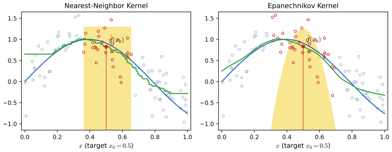
fig_6_1. Reproduces Hastie, Tibshirani and Friedman (2009), Figure 6.1. Download: PDF · SVGResult 6.1 (the three kernels) p. 194, Figure 6.2
Normalised to integrate to one, the three kernels and their constants are
| kernel | normalised \(D(t)\) | \(\mu_2(D)\) | \(R(D)\) | smoothness at the edge of the support |
|---|---|---|---|---|
| Epanechnikov | \(\tfrac34(1-t^2)\) on \([-1,1]\) | \(1/5\) | \(3/5\) | continuous, derivative jumps |
| tri-cube | \(\tfrac{70}{81}(1-|t|^3)^3\) on \([-1,1]\) | \(35/243\) | \(175/247\) | two continuous derivatives |
| Gaussian | \(\phi(t)\) | \(1\) | \(1/(2\sqrt\pi)\) | infinitely differentiable, no edge |
All three are symmetric, so \(\mu_1(D)=\mu_3(D)=0\).
Proof
Epanechnikov. \(\int_{-1}^1\tfrac34(1-t^2)\d t=\tfrac34(2-\tfrac23)=1\); \[\mu_2=\tfrac34\int_{-1}^1(t^2-t^4)\d t=\tfrac34(\tfrac23-\tfrac25)=\tfrac15;\] \[R=\tfrac9{16}\int_{-1}^1(1-2t^2+t^4)\d t=\tfrac9{16}(2-\tfrac43+\tfrac25)=\tfrac9{16}\cdot\tfrac{16}{15}=\tfrac35.\] At \(t=1\) the left derivative is \(-\tfrac32\) and the right derivative is \(0\).
Tri-cube. Expanding \((1-s)^3=1-3s+3s^2-s^3\) with \(s=|t|^3\), \[\int_{-1}^1(1-|t|^3)^3\d t=2(1-\tfrac34+\tfrac37-\tfrac1{10})=\tfrac{81}{70},\] which gives the factor \(70/81\). Similarly \[\int_{-1}^1t^2(1-|t|^3)^3\d t=2(\tfrac13-\tfrac12+\tfrac39-\tfrac1{12})=\tfrac16,\] so \(\mu_2=\tfrac{70}{81}\cdot\tfrac16=\tfrac{35}{243}\); and \[\int_{-1}^1(1-|t|^3)^6\d t=2\sum_{k=0}^6\binom6k\frac{(-1)^k}{3k+1}=\frac{45927}{48412}\approx0.94867;\] multiplying by \((70/81)^2\) gives \(R=175/247\approx0.70850\). Near \(t=1\) put \(s=1-t\): \(1-t^3=3s-3s^2+s^3\), so \(D(t)=27s^3(1+O(s))\); \(D\), \(D'\) and \(D''\) all vanish at the edge and only the third derivative jumps. At \(t=0\), \(|t|^3\) has two continuous derivatives, so the whole kernel is twice continuously differentiable.
Gaussian. \(\mu_2=1\) is the variance of \(N(0,1)\), and \[\int\phi^2=\frac1{2\pi}\int e^{-t^2}\d t=\frac{\sqrt\pi}{2\pi}=\frac1{2\sqrt\pi}.\] ∎
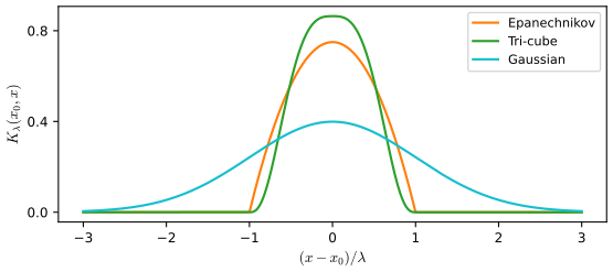
fig_6_2. Reproduces Hastie, Tibshirani and Friedman (2009), Figure 6.2. Download: PDF · SVGThe book lists the practical choices. The width \(\lambda\) has to be chosen (Section 6.2): larger \(\lambda\) averages more points (lower variance) but assumes \(f\) is nearly constant over a wider window (higher bias). A metric window keeps the bias roughly fixed but its variance grows where the data are sparse; a nearest-neighbour window does the opposite. The next box makes this precise.
Filling the gap 6.1: where the bias and the variance go, for metric and nearest-neighbour windows p. 193
Let the \(x_i\) be a sample from a density \(g\), let \(f\) and \(g\) be twice continuously differentiable near an interior point \(x_0\) with \(g(x_0)>0\), and let \(D\) be a symmetric kernel with \(\int D=1\). Then for the Nadaraya–Watson estimator with width \(h\to0\), \(Nh\to\infty\),
\[ \E\hf(x_0)-f(x_0)\approx h^2\mu_2(D)\Big\{\tfrac12f''(x_0)+\frac{f'(x_0)g'(x_0)}{g(x_0)}\Big\},\qquad \Var\hf(x_0)\approx\frac{\sigma^2R(D)}{Nh\,g(x_0)}. \]Derivation, and what it says about the two kinds of window
Write \(\hf(x_0)=A/B\) with \(B=\frac1{Nh}\sum_iD\big(\frac{x_i-x_0}h\big)\) and \(A=\frac1{Nh}\sum_iD\big(\frac{x_i-x_0}h\big)y_i\). Conditionally on the \(x_i\), \(\E(A\given x)=\frac1{Nh}\sum_iD(\cdot)f(x_i)\). Each of these averages is a sum of independent terms whose expectations follow from the substitution \(x=x_0+hu\):
\[ \E B=\int D(u)g(x_0+hu)\d u=g(x_0)+\tfrac12h^2\mu_2g''(x_0)+o(h^2), \] \[ \E\big[\tfrac1{Nh}\textstyle\sum_iD(\cdot)f(x_i)\big]=\int D(u)(fg)(x_0+hu)\d u=(fg)(x_0)+\tfrac12h^2\mu_2(fg)''(x_0)+o(h^2), \]using \(\int D=1\) and \(\int uD=0\) to kill the zero- and first-order terms. Both averages concentrate around these means (their variances are \(O(1/(Nh))\)), so to leading order
\[ \E\hf(x_0)\approx\frac{fg+\tfrac12h^2\mu_2(fg)''}{g+\tfrac12h^2\mu_2g''}\approx f+\tfrac12h^2\mu_2\frac{(fg)''-fg''}{g}=f+\tfrac12h^2\mu_2\frac{f''g+2f'g'}{g}, \]all evaluated at \(x_0\), which is the bias stated. For the variance, conditionally on the \(x_i\), \(\Var\hf(x_0)=\sigma^2\sum_iK_i^2/(\sum_iK_i)^2\) with \(K_i=D((x_i-x_0)/h)\); the sums are \(Nh\{g(x_0)R(D)+o(1)\}\) and \(Nh\{g(x_0)+o(1)\}\), so \(\Var\hf\approx\sigma^2R(D)/(Nhg(x_0))\).
Metric window (\(h=\lambda\) fixed): the variance is inversely proportional to the local density \(g(x_0)\), as the book says. The bias does not involve \(g(x_0)\) itself, but for Nadaraya–Watson it does involve the design through the term \(f'g'/g\); only for local linear regression is the leading bias \(\tfrac12h^2\mu_2f''\) free of the design (Result 6.3), which is where "constant bias" is exactly right.
Nearest-neighbour window: the window around \(x_0\) of half-width \(h\) contains about \(2Nhg(x_0)\) points, so a window holding \(k\) points has \(h_k(x_0)\approx k/(2Ng(x_0))\). Substituting, the variance becomes \(\approx2\sigma^2R(D)/k\), the same everywhere, while the bias becomes \(\approx\mu_2\{\cdot\}k^2/(4N^2g(x_0)^2)\): it varies inversely with the square of the local density (the book's "inversely with local density" describes the direction, not the power). ∎
6.1.1 Local Linear Regression
pp. 194–197 Near the edge of the data a symmetric window becomes one-sided: all the points that get weight lie on one side of \(x_0\). If \(f\) slopes, their responses are systematically higher (or lower) than \(f(x_0)\) and the weighted average is biased (Figure 6.3, left). Fitting a straight line by weighted least squares instead, and evaluating it at \(x_0\), removes this bias to first order.
See also (companion course): Section 3.3.3, the equivalent kernel of Bayesian linear regression.
Definition 6.2 (local linear regression and the equivalent kernel) p. 195, (6.7)–(6.9)
At each target \(x_0\) solve the weighted least-squares problem
\[ \min_{\alpha(x_0),\,\beta(x_0)}\ \sum_{i=1}^NK_\lambda(x_0,x_i)\,\big[y_i-\alpha(x_0)-\beta(x_0)x_i\big]^2 \tag{6.7} \]and set \(\hf(x_0)=\hat\alpha(x_0)+\hat\beta(x_0)x_0\). With \(b(x)^\T=(1,x)\), \(\bB\) the \(N\times2\) matrix with rows \(b(x_i)^\T\) and \(\bW(x_0)=\diag\{K_\lambda(x_0,x_i)\}\),
\[ \hf(x_0)=b(x_0)^\T\big(\bB^\T\bW(x_0)\bB\big)^{-1}\bB^\T\bW(x_0)\by \tag{6.8} \] \[ \phantom{\hf(x_0)}=\sum_{i=1}^Nl_i(x_0)\,y_i. \tag{6.9} \]The weights \(l_i(x_0)\), which do not depend on \(\by\), form the equivalent kernel. The fit is defined when \(\bB^\T\bW\bB\) is invertible, i.e. when at least two distinct \(x_i\) get positive weight.
Result 6.2 (the local linear equivalent kernel and its moments; Exercise 6.2 for \(d=1\)) pp. 195–197
Write \(K_i=K_\lambda(x_0,x_i)\), \(u_i=x_i-x_0\) and \(S_j=\sum_iK_iu_i^j\). Then
\[ l_i(x_0)=K_i\,\frac{S_2-u_iS_1}{S_0S_2-S_1^2},\qquad\sum_{i=1}^Nl_i(x_0)=1,\qquad\sum_{i=1}^N(x_i-x_0)\,l_i(x_0)=0. \]So a local linear fit reproduces every straight line exactly. At an interior point of a symmetric design \(S_1=0\) and \(l_i=K_i/S_0\): the equivalent kernel is the Nadaraya–Watson kernel; where the design is lopsided (\(S_1\ne0\)) it is tilted, and some \(l_i\) can be negative.
Proof
The basis \((1,x)\) and the centred basis \((1,x-x_0)\) span the same functions, and the fitted value at \(x_0\) does not depend on how the line is parametrised; in the centred basis the value at \(x_0\) is the intercept. With \(\bB_0\) having rows \((1,u_i)\),
\[ \bB_0^\T\bW\bB_0=\begin{pmatrix}S_0&S_1\\S_1&S_2\end{pmatrix},\qquad(\bB_0^\T\bW\bB_0)^{-1}=\frac1{S_0S_2-S_1^2}\begin{pmatrix}S_2&-S_1\\-S_1&S_0\end{pmatrix}, \]and \(\hf(x_0)=\be_1^\T(\bB_0^\T\bW\bB_0)^{-1}\bB_0^\T\bW\by\). The first row of the inverse times the \(i\)-th column of \(\bB_0^\T\bW\), which is \(K_i(1,u_i)^\T\), is \(K_i(S_2-S_1u_i)/(S_0S_2-S_1^2)\). Summing, \(\sum_il_i=(S_0S_2-S_1^2)/(S_0S_2-S_1^2)=1\) and \(\sum_iu_il_i=(S_1S_2-S_1S_2)/(S_0S_2-S_1^2)=0\). The denominator is positive by the Cauchy–Schwarz inequality as soon as two distinct \(x_i\) have positive weight. For a line \(y_i=a+bx_i\), \(\sum l_iy_i=(a+bx_0)\sum l_i+b\sum u_il_i=a+bx_0\). Finally \(l_i\lt0\) exactly when \(u_i\) and \(S_1\) have the same sign and \(|u_i|>S_2/|S_1|\): the farthest points on the heavy side of the window are given negative weight. ∎
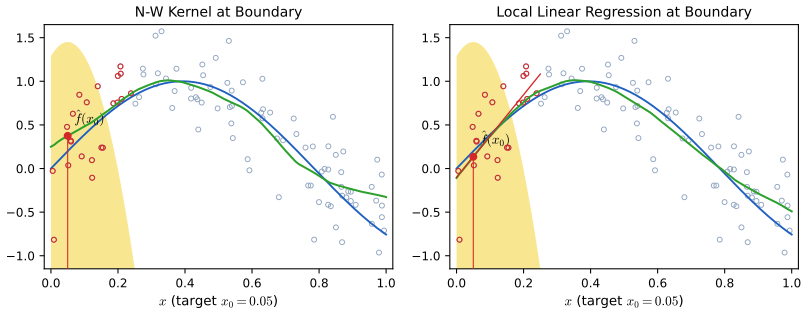
fig_6_3. Reproduces Hastie, Tibshirani and Friedman (2009), Figure 6.3. Download: PDF · SVG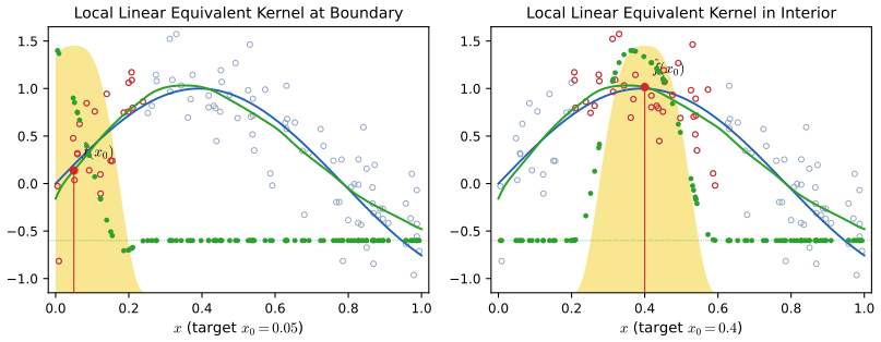
fig_6_4. Reproduces Hastie, Tibshirani and Friedman (2009), Figure 6.4. Download: PDF · SVGThe book calls this automatic kernel carpentry: the old remedy for boundary bias was to design special boundary kernels by asymptotic arguments; local linear regression builds the right kernel at every point, from the actual design. To see what bias remains, expand \(f\) about \(x_0\) and use linearity:
\[ \E\hf(x_0)=\sum_{i=1}^Nl_i(x_0)f(x_i)=f(x_0)\sum_{i=1}^Nl_i(x_0)+f'(x_0)\sum_{i=1}^N(x_i-x_0)l_i(x_0)+\frac{f''(x_0)}{2}\sum_{i=1}^N(x_i-x_0)^2l_i(x_0)+R. \tag{6.10} \]Filling the gap 6.2: the remainder in (6.10) and the bias that is left pp. 196–197
Derivation
If \(f\) has three continuous derivatives on an interval containing the window, Taylor's theorem with the Lagrange remainder gives, for each \(i\) with \(K_i>0\), \[f(x_i)=f(x_0)+f'(x_0)u_i+\tfrac12f''(x_0)u_i^2+\tfrac16f'''(\xi_i)u_i^3\] with \(\xi_i\) between \(x_0\) and \(x_i\). Multiply by \(l_i(x_0)\) and sum (points with \(K_i=0\) have \(l_i=0\)): this is (6.10) with
\[ R=\frac16\sum_{i=1}^Nf'''(\xi_i)\,u_i^3\,l_i(x_0),\qquad|R|\le\frac{\max|f'''|}{6}\,\lambda^3\sum_i|l_i(x_0)| \]for a compact kernel of half-width \(\lambda\). By Result 6.2 the first sum in (6.10) is 1 and the second is 0, so
\[ \E\hf(x_0)-f(x_0)=\frac{f''(x_0)}2\sum_{i=1}^N(x_i-x_0)^2l_i(x_0)+R. \]The bias is exactly zero when \(f\) is linear, and otherwise depends only on second and higher derivatives, whether \(x_0\) is in the interior or on the boundary. For Nadaraya–Watson, by contrast, \(\sum_i(x_i-x_0)l_i=S_1/S_0\), which is of order \(\lambda\) at the boundary, so the bias there is \(f'(x_0)S_1/S_0+O(\lambda^2)\). ∎
Result 6.3 (asymptotic bias and variance in the interior and at the boundary) pp. 194–197
Take a random design with density \(g\) on \([0,1]\), smooth \(f\) and \(g\), a symmetric kernel \(D\) supported on \([-1,1]\) with \(\int D=1\), a metric window \(\lambda\to0\) with \(N\lambda\to\infty\), and the target \(x_0=c\lambda\) near the left boundary (\(0\le c\le1\)); write \(\nu_j=\int_{-c}^1u^jD(u)\d u\). Then
- Nadaraya–Watson: bias \(=\lambda f'(0)\nu_1/\nu_0+O(\lambda^2)\), which is of order \(\lambda\) unless \(c\ge1\) (interior, \(\nu_1=0\));
- local linear: bias \(=\tfrac12\lambda^2f''(0)\,\dfrac{\nu_2^2-\nu_1\nu_3}{\nu_0\nu_2-\nu_1^2}+o(\lambda^2)\), which reduces to \(\tfrac12\lambda^2\mu_2(D)f''(x_0)\) in the interior;
- both: variance \(=\dfrac{\sigma^2}{N\lambda g(0)}\displaystyle\int_{-c}^1K_c^*(u)^2\d u\,(1+o(1))\), with the boundary-adapted kernels \(K_c^*=D/\nu_0\) (Nadaraya–Watson) and \(K_c^*(u)=D(u)\dfrac{\nu_2-\nu_1u}{\nu_0\nu_2-\nu_1^2}\) (local linear).
For the Epanechnikov kernel exactly at the boundary (\(c=0\)): \(\nu_0=\tfrac12\), \(\nu_1=\tfrac3{16}\), \(\nu_2=\tfrac1{10}\), \(\nu_3=\tfrac1{16}\); the Nadaraya–Watson bias is \(\tfrac38\lambda f'(0)\); the local linear bias is \(-\tfrac{11}{95}\cdot\tfrac12\lambda^2f''(0)\); the variance factors \(\int K^{*2}\) are \(1.2\) and \(4.498\), against \(R(D)=0.6\) in the interior.
Proof
For a target \(x_0=c\lambda\), the points with positive weight satisfy \(x_i=x_0+\lambda u\) with \(u\in[-c,1]\). The local sums are \(S_j=\sum_iK_iu_i^j=N\lambda^{j+1}\{g(0)\nu_j+O(\lambda)\}\) (the same substitution as in Filling the gap 6.1, now with the integral cut at \(-c\) because there are no data below 0). For Nadaraya–Watson, \(\sum(x_i-x_0)l_i=S_1/S_0=\lambda\nu_1/\nu_0+O(\lambda^2)\), which multiplies \(f'(x_0)\) in (6.10). For local linear regression Filling the gap 6.2 gives the bias as \(\tfrac12f''(x_0)\sum u_i^2l_i\), and with Result 6.2, \[\sum u_i^2l_i=(S_2^2-S_1S_3)/(S_0S_2-S_1^2)=\lambda^2(\nu_2^2-\nu_1\nu_3)/(\nu_0\nu_2-\nu_1^2)+O(\lambda^3).\] In the interior (\(c\ge1\)) \(\nu_1=\nu_3=0\), \(\nu_0=1\), \(\nu_2=\mu_2\). The variance is \(\sigma^2\sum_il_i^2\), and \(l_i=K^*_c(u_i)/(N\lambda g(0))\,(1+o(1))\), so \(\sum l_i^2=\frac{1}{N\lambda g(0)}\int K_c^{*2}(1+o(1))\). The Epanechnikov numbers are direct integrals of polynomials over \([0,1]\): \(\nu_0=\tfrac12\), \(\nu_1=\tfrac34(\tfrac12-\tfrac14)=\tfrac3{16}\), \(\nu_2=\tfrac34(\tfrac13-\tfrac15)=\tfrac1{10}\), \(\nu_3=\tfrac34(\tfrac14-\tfrac16)=\tfrac1{16}\); then \(\nu_1/\nu_0=\tfrac38\), \[(\nu_2^2-\nu_1\nu_3)/(\nu_0\nu_2-\nu_1^2)=(\tfrac1{100}-\tfrac3{256})/(\tfrac1{20}-\tfrac9{256})=-\tfrac{11}{95},\] \(\int_0^1D^2/\nu_0^2=\tfrac3{10}\cdot4=1.2\), and \(\int_0^1K_0^{*2}\approx4.498\) (computed numerically in the course code). ∎
So at the boundary local linear regression trades a bias of order \(\lambda\) for one of order \(\lambda^2\), at the price of a variance about 3.7 times that of Nadaraya–Watson there (4.498 against 1.2): "a modest cost in variance" for the bias, as the book puts it, compared with what an \(O(\lambda)\) bias costs in mean squared error.
6.1.2 Local Polynomial Regression
pp. 197–198 Why stop at lines? A local polynomial of degree \(d\) solves
\[ \min_{\alpha(x_0),\,\beta_j(x_0),\,j=1,\dots,d}\ \sum_{i=1}^NK_\lambda(x_0,x_i)\Big[y_i-\alpha(x_0)-\sum_{j=1}^d\beta_j(x_0)x_i^j\Big]^2 \tag{6.11} \]with \(\hf(x_0)=\hat\alpha(x_0)+\sum_{j=1}^d\hat\beta_j(x_0)x_0^j\). As before \(\hf(x_0)=\sum_il_i(x_0)y_i\) with \(\bl(x_0)^\T=b(x_0)^\T(\bB^\T\bW\bB)^{-1}\bB^\T\bW\), now with \(b(x)^\T=(1,x,\dots,x^d)\); \(d=0\) is Nadaraya–Watson.
Result 6.4 (moments of the equivalent kernel; Exercise 6.2) p. 197
Let \(b_j(x_0)=\sum_{i=1}^N(x_i-x_0)^jl_i(x_0)\). For local polynomial regression of degree \(d\) (including \(d=0\)), \(b_0(x_0)=1\) and \(b_j(x_0)=0\) for \(j=1,\dots,d\). Consequently, if \(f\) has \(d+1\) continuous derivatives,
\[ \E\hf(x_0)-f(x_0)=\sum_{i=1}^Nl_i(x_0)\,\frac{f^{(d+1)}(\xi_i)}{(d+1)!}(x_i-x_0)^{d+1}, \]so polynomials of degree at most \(d\) are reproduced exactly and the bias involves only derivatives of order \(d+1\) and higher.
Proof
Use the centred basis \(b_0(x)^\T=(1,x-x_0,\dots,(x-x_0)^d)\); it spans the same polynomials as \((1,x,\dots,x^d)\) (the change of basis is an invertible triangular matrix \(\mathbf{T}\), \(\bB=\bB_0\mathbf{T}\), and \[b(x_0)^\T(\bB^\T\bW\bB)^{-1}\bB^\T=b_0(x_0)^\T\mathbf{T}\mathbf{T}^{-1}(\bB_0^\T\bW\bB_0)^{-1}\mathbf{T}^{-\T}\mathbf{T}^\T\bB_0^\T\]), so the fit is unchanged, and \(b_0(x_0)=\be_1\). Hence \(\bl(x_0)^\T=\be_1^\T(\bB_0^\T\bW\bB_0)^{-1}\bB_0^\T\bW\) and
\[ \bl(x_0)^\T\bB_0=\be_1^\T(\bB_0^\T\bW\bB_0)^{-1}\bB_0^\T\bW\bB_0=\be_1^\T. \]The \(j\)-th entry of \(\bl^\T\bB_0\) is \(\sum_il_i(x_i-x_0)^j=b_j(x_0)\), so \(b_0=1\) and \(b_1=\dots=b_d=0\). For the bias, Taylor-expand \(f(x_i)\) to order \(d\) with the Lagrange remainder of order \(d+1\), multiply by \(l_i\) and sum: the terms of order \(1,\dots,d\) vanish and the constant term gives \(f(x_0)\). ∎
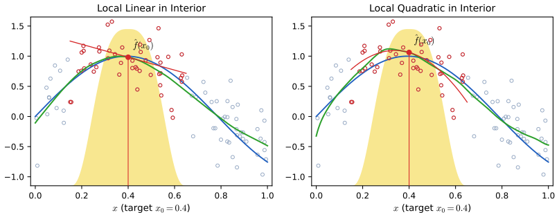
fig_6_5. Reproduces Hastie, Tibshirani and Friedman (2009), Figure 6.5. Download: PDF · SVGIf the errors are independent with variance \(\sigma^2\), then \(\Var\hf(x_0)=\sigma^2\|\bl(x_0)\|^2\). The book states (Exercise 6.3) that \(\|\bl(x_0)\|\) increases with the degree. What is true is the following.
Result 6.5 (the equivalent kernel as a minimum-norm solution, and the variance cost of the degree) p. 197, Exercise 6.3
Let \(\bl^{(d)}(x_0)\) be the equivalent kernel of degree \(d\), and \(\mathcal I=\{i:K_i>0\}\). Then \(\bl^{(d)}\) is the unique minimiser of the weighted norm \(\sum_{i\in\mathcal I}l_i^2/K_i\) among all weight vectors supported on \(\mathcal I\) that satisfy the moment conditions \(\sum_il_i(x_i-x_0)^j=\delta_{j0}\), \(j=0,\dots,d\). Its minimum value \(\be_1^\T(\bB_0^\T\bW\bB_0)^{-1}\be_1\) is therefore nondecreasing in \(d\). In particular:
- for the box kernel (equal weights in the window) \(\|\bl^{(d)}(x_0)\|^2\) is nondecreasing in \(d\);
- for any kernel, the variance \(\sum_il_i^2/K_i\) that the fit would have if \(\Var\varepsilon_i\) were proportional to \(1/K_i\) is nondecreasing in \(d\);
- for a general kernel and equal error variances, \(\|\bl^{(d)}(x_0)\|\) itself can decrease with \(d\) (note below).
Proof
Write the constraints as \(\bB_0^\T\bl=\be_1\) (\(\bB_0\) restricted to the rows in \(\mathcal I\)). The objective \(\bl^\T\bW^{-1}\bl\) is strictly convex, so a minimiser on the affine constraint set is unique if it exists, and it is characterised by the Lagrange condition \(2\bW^{-1}\bl=\bB_0\boldsymbol\nu\) for some \(\boldsymbol\nu\). Then \(\bl=\tfrac12\bW\bB_0\boldsymbol\nu\), and the constraint gives \(\tfrac12\bB_0^\T\bW\bB_0\boldsymbol\nu=\be_1\), so \(\bl=\bW\bB_0(\bB_0^\T\bW\bB_0)^{-1}\be_1\): the equivalent kernel. Its objective value is \[\be_1^\T(\bB_0^\T\bW\bB_0)^{-1}\bB_0^\T\bW\bW^{-1}\bW\bB_0(\bB_0^\T\bW\bB_0)^{-1}\be_1=\be_1^\T(\bB_0^\T\bW\bB_0)^{-1}\be_1.\] Raising the degree from \(d\) to \(d+1\) adds one constraint, so the feasible set shrinks and the minimum cannot decrease. (1): with \(K_i=c\) on \(\mathcal I\), \(\sum l_i^2/K_i=\|\bl\|^2/c\). (2): if \(\Var\varepsilon_i=\tau^2/K_i\), then \(\Var\sum l_iy_i=\tau^2\sum l_i^2/K_i\). (3) is the counterexample below. ∎
Note on the book: Exercise 6.3 is not true as stated
Take the Epanechnikov kernel with \(\lambda=1\), the target \(x_0=0\) and three points \(x=(-0.5,-0.4,0.9)\), with kernel weights \(K=(0.5625,0.63,0.1425)\). Nadaraya–Watson puts almost all of its weight on the two close points: \(\bl^{(0)}=(0.421,0.472,0.107)\), \(\|\bl^{(0)}\|^2=0.4116\). The local line must balance the first moment, which moves weight to the far point: \(\bl^{(1)}=(0.278,0.393,0.329)\), \(\|\bl^{(1)}\|^2=0.3400\), smaller. The variance decreases with the degree. The effect is not confined to contrived designs: on the 100-point design of Figure 6.6 (tri-cube, \(\lambda=0.2\)) the local linear \(\|\bl\|^2\) falls slightly below the Nadaraya–Watson value at some interior targets, by under half a percent. What is true is Result 6.5: the inequality holds for a weighted norm (and for the box kernel), and the curves of Figure 6.6 show the typical behaviour, a large increase near the boundary. The statement in the book's text is safe asymptotically: in the interior the local constant and local linear variances agree to first order, and degree 2 has a strictly larger equivalent-kernel constant.
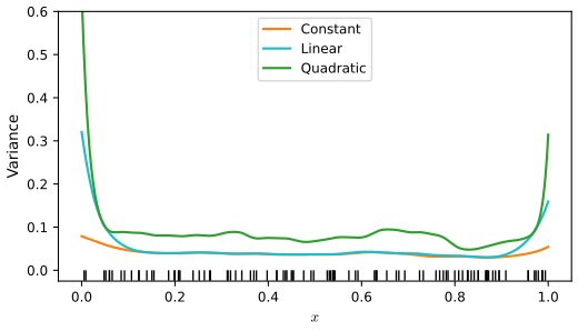
fig_6_6. Reproduces Hastie, Tibshirani and Friedman (2009), Figure 6.6. Download: PDF · SVGFilling the gap 6.3: why odd degrees are preferred p. 198
The book reports that "local polynomials of odd degree dominate those of even degree". Here is the mechanism.
Derivation
In the interior, with a symmetric kernel and a smooth design density, the asymptotic equivalent kernel of degree \(d\) is a fixed function \(K_{(d)}^*\) (the "kernel of order \(d+1\)": the polynomial-times-\(D\) function whose moments \(1,\dots,d\) vanish, from Result 6.4). By symmetry all its odd moments vanish. The leading bias is \(\lambda^{d+1}\frac{f^{(d+1)}}{(d+1)!}\int u^{d+1}K^*_{(d)}\). If \(d\) is even, \(d+1\) is odd and this moment is zero: the bias is of the next order, \(\lambda^{d+2}\), but with a coefficient that involves the design density \(g'/g\), as for Nadaraya–Watson in Filling the gap 6.1. If \(d\) is odd, the bias is of order \(\lambda^{d+1}\) with no design term. Moreover the equivalent kernels of degrees \(2\nu\) and \(2\nu+1\) coincide in the interior (adding the odd term does not change a symmetric problem to first order), so the two have the same asymptotic variance and the same order of bias in the interior. At the boundary the symmetry is lost: the even degree has bias of order \(\lambda^{d+1}\) while the next odd degree, with one more moment condition, has order \(\lambda^{d+2}\). So moving from \(2\nu\) to \(2\nu+1\) costs nothing in the interior and gains an order at the boundary, which is why local linear (\(d=1\)) beats local constant and local cubic beats local quadratic in asymptotic mean squared error (Fan and Gijbels, 1996, Section 3.3). ∎
6.2 Selecting the Width of the Kernel
pp. 198–200 For the Epanechnikov or tri-cube kernel with a metric window \(\lambda\) is the radius of the support; for the Gaussian kernel it is the standard deviation; for nearest-neighbour windows it is \(k\), often given as the span \(k/N\). A narrow window averages few points close to \(x_0\) (low bias, variance close to that of a single \(y_i\)); a wide window averages many points, some far away (low variance, higher bias). As \(\lambda\to0\) a local linear fit tends to the piecewise-linear interpolant of the data (for uniformly spaced \(x_i\)); as \(\lambda\to\infty\) every weight tends to the same value and the fit tends to the global least-squares line.
Definition 6.3 (smoother matrix and effective degrees of freedom) p. 199
Evaluated at the training points, a local polynomial fit is \(\hat\bf=\bS_\lambda\by\) with \(\{\bS_\lambda\}_{ij}=l_j(x_i)\): row \(i\) is the equivalent kernel at \(x_i\). The effective degrees of freedom are \(\mathrm{df}_\lambda=\Tr(\bS_\lambda)\).
Result 6.6 (leave-one-out cross-validation in one fit; Exercise 6.7) p. 199
For local polynomial regression with a metric window, let \(\hf^{(-i)}(x_i)\) be the fit at \(x_i\) computed without the \(i\)-th observation (and with the same kernel weights for the others). If \(\bB_0^\T\bW(x_i)\bB_0\) stays invertible when point \(i\) is removed, then \(S_{ii}\lt1\) and
\[ y_i-\hf^{(-i)}(x_i)=\frac{y_i-\hf(x_i)}{1-S_{ii}},\qquad\mathrm{CV}(\lambda)=\frac1N\sum_{i=1}^N\Big(\frac{y_i-\hf(x_i)}{1-S_{ii}}\Big)^2. \]Proof
Fix \(i\) and the target \(x_i\). Let \(\hat\beta^{(-i)}\) minimise \(Q_{-i}(\beta)=\sum_{j\ne i}K_j(y_j-b_0(x_j)^\T\beta)^2\) (centred at \(x_i\)), and \(z=\hf^{(-i)}(x_i)=b_0(x_i)^\T\hat\beta^{(-i)}\) (the intercept). Define \(\by^*\) as \(\by\) with \(y_i\) replaced by \(z\). The full weighted criterion on \(\by^*\) is \[Q_{-i}(\beta)+K_i(z-b_0(x_i)^\T\beta)^2\ge Q_{-i}(\beta)\ge Q_{-i}(\hat\beta^{(-i)}),\] and both inequalities are equalities at \(\beta=\hat\beta^{(-i)}\); so \(\hat\beta^{(-i)}\) also minimises the full criterion on \(\by^*\), and by uniqueness the full fit at \(x_i\) on \(\by^*\) is \(z\). By linearity that fit is \(\sum_jS_{ij}y_j^*=\hf(x_i)-S_{ii}y_i+S_{ii}z\). Hence \(z(1-S_{ii})=\hf(x_i)-S_{ii}y_i\), and
\[ y_i-z=\frac{y_i(1-S_{ii})-\hf(x_i)+S_{ii}y_i}{1-S_{ii}}=\frac{y_i-\hf(x_i)}{1-S_{ii}}. \]\(S_{ii}\lt1\): by Result 6.5, \(S_{ii}=l_i(x_i)=K_i\,\be_1^\T(\bB_0^\T\bW\bB_0)^{-1}b_0(x_i)\), and the leverage of a point in a weighted least-squares fit is below one exactly when the fit without it is still determined. The argument uses that removing point \(i\) does not change the other points' weights, which holds for a metric window. With a nearest-neighbour window, deleting a point changes the \(k\)-th neighbour and therefore the weights, and the formula becomes an approximation. ∎
Generalised cross-validation replaces each \(S_{ii}\) by the average \(\Tr(\bS_\lambda)/N\): \[\mathrm{GCV}(\lambda)=\frac1N\sum_i(y_i-\hf(x_i))^2/(1-\Tr\bS_\lambda/N)^2.\] Mallows' \(C_p\) is the subject of Exercise 6.10:
Result 6.7 (\(C_p\) for a linear smoother; Exercise 6.10) pp. 199, 217–218, (6.34)–(6.35)
Let \(y_i=f(x_i)+\varepsilon_i\) with fixed \(x_i\) and independent errors of mean 0 and variance \(\sigma^2\), \(\hat\bf=\bS_\lambda\by\), and let \(y_i^*\) be new responses at the same \(x_i\), independent of \(\by\). With the in-sample prediction error
\[ \PE(\lambda)=\E\,\frac1N\sum_{i=1}^N\big(y_i^*-\hf_\lambda(x_i)\big)^2 \tag{6.34} \]and the average squared residual \(\ASR(\lambda)=\frac1N\sum_i(y_i-\hf_\lambda(x_i))^2\),
\[ \E\ASR(\lambda)=\PE(\lambda)-\frac{2\sigma^2}N\Tr(\bS_\lambda),\qquad C_\lambda=\ASR(\lambda)+\frac{2\sigma^2}N\Tr(\bS_\lambda) \tag{6.35} \]is unbiased for \(\PE(\lambda)\). The training error is optimistic by \(2\sigma^2\mathrm{df}_\lambda/N\).
Proof
Write \(\by=\bf+\boldsymbol\varepsilon\), \(\bf=(f(x_i))_i\). For any fixed matrix \(\mathbf{M}\) and vector \(\mathbf{a}\), \[\E\|\mathbf{a}+\mathbf{M}\boldsymbol\varepsilon\|^2=\|\mathbf{a}\|^2+\sigma^2\Tr(\mathbf{M}^\T\mathbf{M}).\] Residuals: \[\by-\bS\by=(\mathbf{I}-\bS)\bf+(\mathbf{I}-\bS)\boldsymbol\varepsilon,\] so
\[ N\,\E\ASR=\|(\mathbf{I}-\bS)\bf\|^2+\sigma^2\Tr\{(\mathbf{I}-\bS)^\T(\mathbf{I}-\bS)\}=\|(\mathbf{I}-\bS)\bf\|^2+\sigma^2\{N-2\Tr\bS+\Tr(\bS^\T\bS)\}. \]Prediction: \[\by^*-\bS\by=(\mathbf{I}-\bS)\bf+\boldsymbol\varepsilon^*-\bS\boldsymbol\varepsilon\] with \(\boldsymbol\varepsilon^*\) independent of \(\boldsymbol\varepsilon\), so the cross term has mean zero and
\[ N\,\PE=\|(\mathbf{I}-\bS)\bf\|^2+N\sigma^2+\sigma^2\Tr(\bS^\T\bS). \]Subtracting, \(N(\PE-\E\ASR)=2\sigma^2\Tr\bS\), which is the claim; \(\E C_\lambda=\PE(\lambda)\) follows. ∎
Filling the gap 6.4: the optimal width and its rate pp. 198–199
Derivation
For local linear regression in the interior, Result 6.3 gives the pointwise mean squared error \[\mathrm{MSE}(x_0)\approx\tfrac14\lambda^4\mu_2^2f''(x_0)^2+\sigma^2R(D)/(N\lambda g(x_0)).\] Integrate against \(g\) to get the average error over the design,
\[ \mathrm{AMISE}(\lambda)=\frac{\lambda^4\mu_2^2}{4}\int f''(x)^2g(x)\,\d x+\frac{\sigma^2R(D)\,|\mathcal X|}{N\lambda}, \]where \(|\mathcal X|\) is the length of the design interval. The first term increases and the second decreases with \(\lambda\). Setting the derivative to zero, \(\lambda^3\mu_2^2\int f''^2g=\sigma^2R|\mathcal X|/(N\lambda^2)\), so
\[ \lambda_{\rm opt}=\Big(\frac{\sigma^2R(D)\,|\mathcal X|}{\mu_2^2\int f''^2g}\Big)^{1/5}N^{-1/5},\qquad\mathrm{AMISE}(\lambda_{\rm opt})\propto N^{-4/5}. \]The optimal width shrinks slowly, the error decreases more slowly than the parametric \(N^{-1}\), and \(\lambda_{\rm opt}\) depends on unknown quantities (\(\sigma^2\), \(\int f''^2g\)): hence data-based choices (cross-validation, GCV, \(C_p\)), or plug-in estimates of these quantities. The effective degrees of freedom calibrate different smoothers against each other: for a metric window in the interior \(S_{ii}\approx D(0)/(N\lambda g(x_i))\), so \(\Tr\bS_\lambda\approx D(0)|\mathcal X|/\lambda\) grows like \(1/\lambda\). ∎
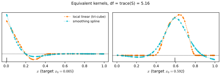
fig_6_7 (the spline is scipy.interpolate.make_smoothing_spline, its smoother matrix built column by column). Reproduces Hastie, Tibshirani and Friedman (2009), Figure 6.7. Download: PDF · SVGThe demonstration computes \(\Tr\bS_\lambda\) and the leave-one-out error for any kernel, degree and width; try the width slider on preset 2 and watch the two numbers move in opposite directions.
6.3 Local Regression in \(\R^p\)
pp. 200–201 The construction extends directly. Let \(b(X)\) collect the monomials of degree at most \(d\) in the \(p\) inputs (for \(p=2\): \((1,X_1,X_2)\) for \(d=1\), and \((1,X_1,X_2,X_1^2,X_2^2,X_1X_2)\) for \(d=2\)).
Definition 6.4 (local polynomial regression in \(\R^p\)) p. 200, (6.12)–(6.13)
At each \(x_0\in\R^p\) solve
\[ \min_{\beta(x_0)}\ \sum_{i=1}^NK_\lambda(x_0,x_i)\big(y_i-b(x_i)^\T\beta(x_0)\big)^2 \tag{6.12} \]and set \(\hf(x_0)=b(x_0)^\T\hat\beta(x_0)\), usually with a radial kernel
\[ K_\lambda(x_0,x)=D\Big(\frac{\|x-x_0\|}{\lambda}\Big). \tag{6.13} \]Because the Euclidean norm mixes units, the inputs are usually standardised first.
Result 6.8 (local linear regression in \(\R^p\) reproduces planes) p. 200
For \(d=1\), \(\hf(x_0)=\sum_il_i(x_0)y_i\) with \(\sum_il_i=1\) and \(\sum_il_i(x_i-x_0)=\mathbf 0\in\R^p\). Hence if \(f\) is twice continuously differentiable with Hessian \(\mathbf H\),
\[ \E\hf(x_0)-f(x_0)=\tfrac12\sum_il_i(x_0)\,(x_i-x_0)^\T\mathbf H(\xi_i)(x_i-x_0), \]a second-order quantity, at interior and boundary points alike and whatever the shape of the boundary.
Proof
Exactly as in Result 6.4: in the centred basis \((1,(x-x_0)^\T)\), \(\bl^\T\bB_0=\be_1^\T\) says \(\sum l_i=1\) and \(\sum l_i(x_i-x_0)=\mathbf 0\). Taylor's theorem in several variables, \[f(x_i)=f(x_0)+\nabla f(x_0)^\T(x_i-x_0)+\tfrac12(x_i-x_0)^\T\mathbf H(\xi_i)(x_i-x_0),\] multiplied by \(l_i\) and summed, gives the bias. No property of the window's shape was used: the correction is automatic for irregular boundaries such as the star-shaped design of Figure 6.8. ∎
Filling the gap 6.5: the boundary and the curse of dimensionality p. 200
Derivation
The boundary grows. For \(N\) points uniform on \([0,1]^p\), a point is within \(\varepsilon\) of the boundary unless all its coordinates lie in \([\varepsilon,1-\varepsilon]\), which has probability \((1-2\varepsilon)^p\). The fraction near the boundary, \(1-(1-2\varepsilon)^p\), tends to one as \(p\) grows: for \(\varepsilon=0.05\) it is 10% when \(p=1\), 41% when \(p=5\) and 88% when \(p=20\). So boundary effects, which local linear regression corrects, dominate in high dimensions.
Localness and sample size cannot both be kept. A cubical neighbourhood of side \(r\) captures a fraction \(r^p\) of uniform data; to hold \(k\) points it needs \(r=(k/N)^{1/p}\), which approaches 1 (not local at all) as \(p\) grows unless \(N\) grows exponentially in \(p\). Quantitatively, the variance of a local linear fit is \(\propto1/(N\lambda^p)\) and its bias \(\propto\lambda^2\); balancing gives \(\lambda\propto N^{-1/(p+4)}\) and a mean squared error of order \(N^{-4/(p+4)}\): with \(p=10\), multiplying the sample size by 1000 reduces the error only by a factor \(1000^{4/14}\approx7\). ∎
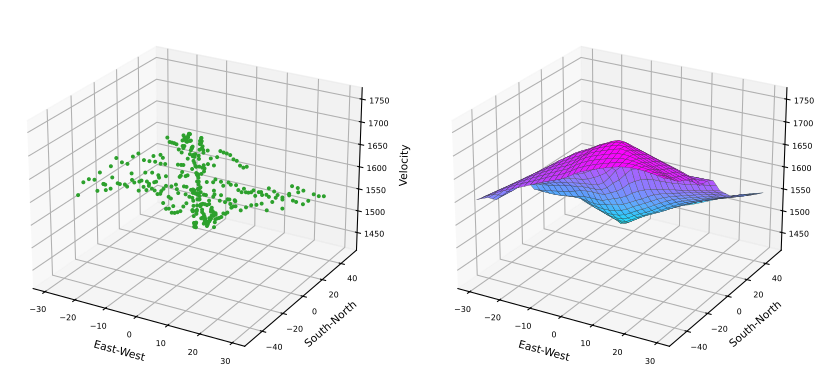
fig_6_8, local_linear_2d. Reproduces Hastie, Tibshirani and Friedman (2009), Figure 6.8. Download: PDF · SVGPictures like the right panel are hard to read beyond the gross shape. Conditioning plots are more useful: show the response against one input in panels that each hold the data with the other inputs in a given range. Conditioning on a range is itself a kind of localisation, so each panel is a one-dimensional local regression.
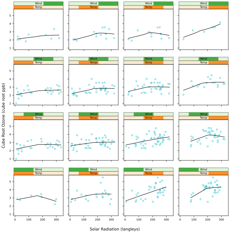
fig_6_9. Reproduces Hastie, Tibshirani and Friedman (2009), Figure 6.9. Download: PDF · SVG6.4 Structured Local Regression Models in \(\R^p\)
p. 201 When the dimension is high relative to \(N\), local regression helps only with structural assumptions. Two kinds are discussed: structure in the kernel, and structure in the regression function.
6.4.1 Structured Kernels
p. 203 Replace the spherical kernel (6.13) by one built on a positive semidefinite matrix \(\bA\):
\[ K_{\lambda,\bA}(x_0,x)=D\Big(\frac{(x-x_0)^\T\bA(x-x_0)}{\lambda}\Big). \tag{6.14} \]Filling the gap 6.6: what the matrix \(\bA\) does p. 203
Derivation
Write \(\bA=\mathbf{L}^\T\mathbf{L}\) (for example \(\mathbf L=\bA^{1/2}\)). Then \((x-x_0)^\T\bA(x-x_0)=\|\mathbf Lx-\mathbf Lx_0\|^2\): the structured kernel is an ordinary radial kernel applied to the transformed inputs \(z=\mathbf Lx\). If \(\bA\) is diagonal, \(A_{jj}\) rescales input \(j\): a large \(A_{jj}\) makes the kernel narrow in that direction (the input matters a lot) and \(A_{jj}=0\) makes the kernel constant along it (the input is ignored). If \(\bA\) has rank \(r\lt p\), the weights depend on \(x\) only through the \(r\) linear combinations \(\mathbf Lx\); a local constant fit with such a kernel is a function of \(\mathbf Lx\) alone, a sum of ridge functions in the projection-pursuit sense of Chapter 11 when \(\mathbf L\) is learned. The choice \(\bA=\Sigma^{-1}\) gives the Mahalanobis distance; Exercise 6.4 shows why that can be a poor choice for smooth signals. ∎
6.4.2 Structured Regression Functions
pp. 203–205 An analysis-of-variance decomposition writes the regression function as main effects, two-way interactions and so on,
\[ f(X_1,X_2,\dots,X_p)=\alpha+\sum_jg_j(X_j)+\sum_{k\lt\ell}g_{k\ell}(X_k,X_\ell)+\cdots, \tag{6.15} \]and structure means dropping the higher-order terms. In the additive model \(f=\alpha+\sum_jg_j(X_j)\), if all terms but \(g_k\) are known, \(g_k\) is estimated by a one-dimensional local regression of the partial residual \(Y-\sum_{j\ne k}g_j(X_j)\) on \(X_k\); cycling over \(k\) until convergence is backfitting (Chapter 9). An important special case is the varying-coefficient model.
Definition 6.5 (varying-coefficient model) p. 204, (6.16)–(6.17)
Split the inputs into \((X_1,\dots,X_q)\) and the rest, \(Z\). The model is conditionally linear,
\[ f(X)=\alpha(Z)+\beta_1(Z)X_1+\cdots+\beta_q(Z)X_q, \tag{6.16} \]and is fitted at each \(z_0\) by weighted least squares with a kernel in \(z\) only:
\[ \min_{\alpha(z_0),\,\beta(z_0)}\ \sum_{i=1}^NK_\lambda(z_0,z_i)\big(y_i-\alpha(z_0)-x_{1i}\beta_1(z_0)-\cdots-x_{qi}\beta_q(z_0)\big)^2. \tag{6.17} \]Result 6.9 (the varying-coefficient fit, its local linear refinement and its standard errors)
Let \(\mathbf X\) be the \(N\times(q+1)\) matrix with rows \((1,x_{1i},\dots,x_{qi})\) and \(\bW(z_0)=\diag\{K_\lambda(z_0,z_i)\}\). The solution of (6.17) is \[\hat\theta(z_0)=(\mathbf X^\T\bW\mathbf X)^{-1}\mathbf X^\T\bW\by=\mathbf L(z_0)\by,\] linear in \(\by\). Adding the columns \(\mathbf X\,\diag(z_i-z_0)\) (each coefficient locally linear in \(z\)) and keeping the first \(q+1\) coefficients removes the first-order bias in \(z\), as in Result 6.2. With independent errors of variance \(\sigma^2\), \(\Cov\hat\theta(z_0)=\sigma^2\mathbf L(z_0)\mathbf L(z_0)^\T\), and \(\sigma^2\) is estimated by \(\mathrm{RSS}/(N-2\Tr\bS+\Tr\bS^\T\bS)\), where \(\bS\) maps \(\by\) to the fitted values \(\hf(x_i,z_i)\).
Proof
(6.17) is a weighted least-squares problem in \(\theta=(\alpha,\beta_1,\dots,\beta_q)\) with design \(\mathbf X\); its normal equations are \(\mathbf X^\T\bW\mathbf X\theta=\mathbf X^\T\bW\by\). With the extra columns the design is \([\mathbf X,\ \mathbf X\diag(z_i-z_0)]\) and the model says \(\theta(z_i)\approx\theta(z_0)+\theta'(z_0)(z_i-z_0)\); the coefficients of the first block estimate \(\theta(z_0)\), and the argument of Result 6.4, applied coordinate by coordinate, shows that a coefficient function that is linear in \(z\) is reproduced exactly. Covariance: \(\hat\theta=\mathbf L\by\) and \(\Cov\by=\sigma^2\mathbf I\). For \(\sigma^2\): with fitted values \(\bS\by\), \[\E\,\mathrm{RSS}=\|(\mathbf I-\bS)\bf\|^2+\sigma^2\Tr\{(\mathbf I-\bS)^\T(\mathbf I-\bS)\}\] (proof of Result 6.7); ignoring the bias term, \(\E\,\mathrm{RSS}\approx\sigma^2(N-2\Tr\bS+\Tr\bS^\T\bS)\). ∎
About Figures 6.10 and 6.11
The book illustrates (6.17) with measurements of the diameter of the human aorta, modelled as linear in age with coefficients that vary with depth down the aorta and with gender. Those data are not distributed with the book, so the two figures are not reproduced. Figure 6.S1 shows the same kind of analysis on one of the book's own data sets.
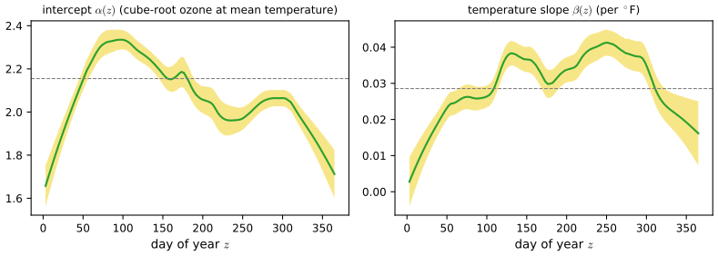
fig_6_s1, varying_coefficient. Stands in for Hastie, Tibshirani and Friedman (2009), Figures 6.10–6.11. Download: PDF · SVG6.5 Local Likelihood and Other Models
pp. 205–208 Any parametric model whose fitting procedure accepts observation weights can be made local. If each observation has a parameter \(\theta_i=\theta(x_i)=x_i^\T\beta\) and inference uses the log-likelihood \(l(\beta)=\sum_il(y_i,x_i^\T\beta)\), the local likelihood at \(x_0\) is
\[ l(\beta(x_0))=\sum_{i=1}^NK_\lambda(x_0,x_i)\,l\big(y_i,x_i^\T\beta(x_0)\big), \]and \(\theta(x_0)=x_0^\T\hat\beta(x_0)\). The kernel can also live on different variables from the model, \(l(\theta(z_0))=\sum_iK_\lambda(z_0,z_i)l(y_i,\eta(x_i,\theta(z_0)))\), giving varying-coefficient generalised linear models; and an autoregressive model \(y_t=\beta_0+\beta_1y_{t-1}+\cdots+\beta_ky_{t-k}+\varepsilon_t\), fitted by local least squares with a kernel \(K(z_0,z_t)\) on the lag vector \(z_t=(y_{t-1},\dots,y_{t-k})\), lets the dynamics depend on the recent history of the series.
Definition 6.6 (local multiclass logistic regression) pp. 206–207, (6.18)–(6.20)
The linear logistic model for \(J\) classes (Section 4.4) is
\[ \Pr(G=j\given X=x)=\frac{e^{\beta_{j0}+\beta_j^\T x}}{1+\sum_{k=1}^{J-1}e^{\beta_{k0}+\beta_k^\T x}}. \tag{6.18} \]Its local version maximises, at each \(x_0\),
\[ \sum_{i=1}^NK_\lambda(x_0,x_i)\Big\{\beta_{g_i0}(x_0)+\beta_{g_i}(x_0)^\T(x_i-x_0)-\log\Big[1+\sum_{k=1}^{J-1}\exp\big(\beta_{k0}(x_0)+\beta_k(x_0)^\T(x_i-x_0)\big)\Big]\Big\}, \tag{6.19} \]with \(\beta_{J0}=0\), \(\beta_J=\mathbf 0\). Because the regressions are centred at \(x_0\), the fitted probabilities at \(x_0\) involve only the intercepts:
\[ \hat\Pr(G=j\given X=x_0)=\frac{e^{\hat\beta_{j0}(x_0)}}{1+\sum_{k=1}^{J-1}e^{\hat\beta_{k0}(x_0)}}. \tag{6.20} \]Result 6.10 (Newton's method for the local logistic likelihood) pp. 206–207
For two classes (\(y_i\in\{0,1\}\)) and local regressors \(b_i=(1,x_i-x_0)\), the local log-likelihood \(\ell(\beta)=\sum_iK_i\{y_ib_i^\T\beta-\log(1+e^{b_i^\T\beta})\}\) has gradient and Hessian
\[ \nabla\ell=\sum_iK_i(y_i-p_i)b_i,\qquad\nabla^2\ell=-\sum_iK_ip_i(1-p_i)b_ib_i^\T,\qquad p_i=\frac{1}{1+e^{-b_i^\T\beta}}. \]\(\ell\) is concave, strictly so when the points with \(K_i>0\) include two distinct \(x_i\); the Newton step \[\beta\leftarrow\beta+(\sum K_ip_i(1-p_i)b_ib_i^\T)^{-1}\sum K_i(y_i-p_i)b_i\] is a weighted least-squares fit (iteratively reweighted least squares) with weights \(K_ip_i(1-p_i)\). The maximiser exists and is unique unless the weighted data are separable by a point (all cases on one side of some threshold within the window), in which case the slope diverges.
Proof
\(\frac{\d}{\d\eta}\{y\eta-\log(1+e^\eta)\}=y-\sigma(\eta)\) and \(\frac{\d^2}{\d\eta^2}=-\sigma(\eta)(1-\sigma(\eta))\), and \(\eta_i=b_i^\T\beta\) is linear in \(\beta\); the chain rule gives the gradient and Hessian. For any \(v\), \(v^\T\nabla^2\ell\,v=-\sum K_ip_i(1-p_i)(b_i^\T v)^2\le0\), with equality only if \(b_i^\T v=0\) for every \(i\) with \(K_i>0\), impossible for \(v\ne0\) when two distinct \(x_i\) carry weight. Writing the Newton step as \[\beta^{\rm new}=(\mathbf B^\T\mathbf V\mathbf B)^{-1}\mathbf B^\T\mathbf V\mathbf z\] with \(\mathbf V=\diag(K_ip_i(1-p_i))\) and working response \(z_i=b_i^\T\beta+(y_i-p_i)/(p_i(1-p_i))\) shows it is a weighted least-squares fit, as for global logistic regression (Section 4.4.1 of the book). Existence: if no \(v\) makes \(\ell\) increase without bound along \(\beta+tv\), the concave \(\ell\) attains its supremum; such a direction exists exactly when \(\{y_i=1\}\) and \(\{y_i=0\}\) (restricted to \(K_i>0\)) are separated by a threshold, the one-dimensional version of separability. In Figure 6.12 the windows are wide enough that this never happens; Newton's method converges in at most five iterations from \(\beta=(\logit\bar y_w,0)\). ∎
See also (companion course): Section 4.3.3, iterative reweighted least squares for the global model.
Filling the gap 6.7: standard errors for local likelihood estimates pp. 207–208
The book draws "estimated pointwise standard-error bands" in Figure 6.12 without saying how. Here is the standard construction.
Derivation
The local estimate solves the weighted score equation \(U(\beta)=\sum_iK_i(y_i-p_i(\beta))b_i=0\). Let \(\beta^*\) solve \(\E U(\beta^*)=0\) (the target of the local fit) and expand: \(0=U(\hat\beta)\approx U(\beta^*)-\mathbf A(\hat\beta-\beta^*)\) with \(\mathbf A=\sum_iK_ip_i(1-p_i)b_ib_i^\T\), the negative Hessian. So \(\hat\beta-\beta^*\approx\mathbf A^{-1}U(\beta^*)\). The \(y_i\) are independent Bernoulli, so \[\Var U=\sum_iK_i^2\Var(y_i)b_ib_i^\T\approx\sum_iK_i^2p_i(1-p_i)b_ib_i^\T=\mathbf B.\] Therefore
\[ \Cov\hat\beta\approx\mathbf A^{-1}\mathbf B\mathbf A^{-1}, \]the "sandwich". Unlike global maximum likelihood, \(\mathbf B\ne\mathbf A\): the weights enter \(\mathbf A\) once and \(\mathbf B\) twice, because the kernel is a device for localisation, not a model for the variance. The standard error of \(\hat\eta(x_0)=\hat\beta_0\) is \(\sqrt{(\mathbf A^{-1}\mathbf B\mathbf A^{-1})_{11}}\), and the band on the probability scale is \(\sigma(\hat\eta\pm\mathrm{se})\), which stays inside \([0,1]\). This band reflects variance only; it ignores the smoothing bias. ∎
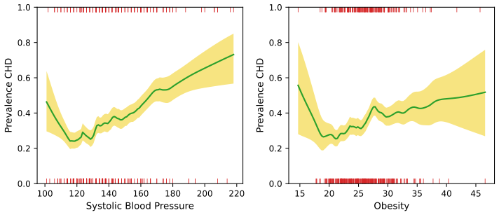
fig_6_12, local_logistic. Reproduces Hastie, Tibshirani and Friedman (2009), Figure 6.12. Download: PDF · SVGBecause CHD is binary one could simply smooth the 0/1 response with a kernel. That is the local constant version of (6.19):
Result 6.11 (a local constant logit is a Nadaraya–Watson smooth of the indicators; Exercise 6.5) p. 207
If in (6.19) only the intercepts are kept (\(\beta_j(x_0)=\mathbf 0\)), the maximiser satisfies
\[ \hat\Pr(G=j\given X=x_0)=\frac{\sum_iK_\lambda(x_0,x_i)\,\mathbf 1(g_i=j)}{\sum_iK_\lambda(x_0,x_i)},\qquad j=1,\dots,J, \]the Nadaraya–Watson smooth (6.2) of the class indicators, whenever every class has positive kernel weight at \(x_0\).
Proof
With intercepts only, write \(p_j=e^{\beta_{j0}}/(1+\sum_{k\lt J}e^{\beta_{k0}})\) (\(\beta_{J0}=0\)); (6.19) becomes \(\sum_iK_i\log p_{g_i}=\sum_jn_j\log p_j\) with \(n_j=\sum_iK_i\mathbf 1(g_i=j)\). The map from \((\beta_{10},\dots,\beta_{J-1,0})\in\R^{J-1}\) to probability vectors with all entries positive is a bijection, so we may maximise \(\sum_jn_j\log p_j\) over the simplex. With a Lagrange multiplier for \(\sum p_j=1\): \(n_j/p_j=\mu\), so \(p_j=n_j/\sum_kn_k\). (Equivalently, the score for \(\beta_{j0}\) is \(\sum_iK_i\{\mathbf 1(g_i=j)-p_j\}=0\).) If some \(n_j=0\) the supremum is approached as \(\beta_{j0}\to-\infty\), consistent with the smoother giving \(0\). ∎
Smoothing the indicators directly has the boundary bias of the Nadaraya–Watson average; working on the unrestricted logit scale with a local line keeps the bias correction of local linear regression and guarantees fitted probabilities in \((0,1)\).
6.6 Kernel Density Estimation and Classification
p. 208 Kernel density estimation is unsupervised and historically precedes kernel regression; it leads directly to nonparametric classifiers.
See also (companion courses): Section 2.5.1 of Bayesian and Probabilistic Machine Learning; Section 3.5.2 of Foundations of Deep Learning.
6.6.1 Kernel Density Estimation
Definition 6.7 (kernel density estimate) pp. 208–209, (6.21)–(6.24)
For a sample \(x_1,\dots,x_N\) from a density \(f_X\) on \(\R\), the local count in a window \(\mathcal N(x_0)\) of width \(\lambda\) gives
\[ \hf_X(x_0)=\frac{\#\{x_i\in\mathcal N(x_0)\}}{N\lambda}, \tag{6.21} \]and the smooth Parzen estimate is
\[ \hf_X(x_0)=\frac1{N\lambda}\sum_{i=1}^NK_\lambda(x_0,x_i). \tag{6.22} \]With the Gaussian kernel \(K_\lambda(x_0,x)=\phi(|x-x_0|/\lambda)\) and \(\phi_\lambda\) the \(N(0,\lambda^2)\) density,
\[ \hf_X(x)=\frac1N\sum_{i=1}^N\phi_\lambda(x-x_i)=(\hat F\star\phi_\lambda)(x), \tag{6.23} \]the convolution of the empirical distribution \(\hat F\) (mass \(1/N\) at each \(x_i\)) with \(\phi_\lambda\): the density of \(x_I+\lambda Z\) with \(I\) uniform on \(\{1,\dots,N\}\) and \(Z\sim N(0,1)\). In \(\R^p\) the Gaussian product kernel gives
\[ \hf_X(x_0)=\frac1{N(2\lambda^2\pi)^{p/2}}\sum_{i=1}^Ne^{-\frac12(\|x_i-x_0\|/\lambda)^2}. \tag{6.24} \]The definitions (6.21) and (6.22) are densities: \(\int\hf_X=1\) whenever \(\int D=1\), because each term \(\frac1\lambda D((x-x_i)/\lambda)\) integrates to one.
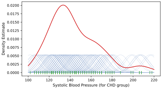
fig_6_13. Reproduces Hastie, Tibshirani and Friedman (2009), Figure 6.13. Download: PDF · SVGResult 6.12 (bias, variance and the AMISE bandwidth) p. 208; Silverman (1986), Section 3.3
Let \(\hf(x)=\frac1{N\lambda}\sum_iD((x-x_i)/\lambda)\) with \(D\) a symmetric density with finite \(\mu_2(D)\) and \(R(D)\), and \(f\) with a square-integrable, continuous second derivative. As \(\lambda\to0\), \(N\lambda\to\infty\):
\[ \E\hf(x)-f(x)=\tfrac12\lambda^2\mu_2f''(x)+o(\lambda^2),\qquad\Var\hf(x)=\frac{R(D)f(x)}{N\lambda}+o\Big(\frac1{N\lambda}\Big), \] \[ \MISE(\lambda)=\E\!\int(\hf-f)^2=\frac{R(D)}{N\lambda}+\frac{\lambda^4\mu_2^2R(f'')}{4}+o\Big(\frac1{N\lambda}+\lambda^4\Big), \]minimised (in its leading terms) by
\[ \lambda_{\rm AMISE}=\Big(\frac{R(D)}{\mu_2^2R(f'')N}\Big)^{1/5}. \]If \(f\) is the \(N(\mu,s^2)\) density and \(D=\phi\), \(R(f'')=3/(8\sqrt\pi s^5)\) and \(\lambda_{\rm AMISE}=(4/3)^{1/5}sN^{-1/5}\approx1.06\,sN^{-1/5}\), the normal-reference rule.
Proof sketch (pointwise part in the companion course)
The pointwise bias and variance are proved in the companion course, Result 2.26: substitute \(y=x-\lambda u\) in \(\E\hf(x)=\int D(u)f(x-\lambda u)\d u\) and expand to second order; the variance of an average of \(N\) independent terms is \(\frac1N\Var\{\lambda^{-1}D((x-X)/\lambda)\}\). Integrating over \(x\): \(\int\Var\hf\approx\frac{R(D)}{N\lambda}\int f=\frac{R(D)}{N\lambda}\) and \(\int\mathrm{bias}^2\approx\frac{\lambda^4\mu_2^2}4\int f''^2\). Minimising \(a/\lambda+b\lambda^4\) gives \(\lambda^5=a/(4b)\), which is the formula. For the normal density with variance \(s^2\), \(f''(x)=f(x)(z^2-1)/s^2\) with \(z=(x-\mu)/s\), so \[R(f'')=\frac1{s^4}\int f^2(z^2-1)^2\d x=\frac1{2\pi s^5}\int e^{-z^2}(z^4-2z^2+1)\d z=\frac{\sqrt\pi}{2\pi s^5}(\tfrac34-1+1)=\frac3{8\sqrt\pi s^5}.\] With \(R(\phi)=1/(2\sqrt\pi)\) and \(\mu_2=1\): \(\lambda^5=\frac{1/(2\sqrt\pi)}{3/(8\sqrt\pi s^5)N}=\frac43s^5N^{-1}\). Silverman's rule \(0.9\min(s,\mathrm{IQR}/1.34)N^{-1/5}\) lowers the constant and uses a robust scale, so that skewed or two-peaked densities are smoothed less. ∎
Result 6.13 (least-squares cross-validation; Rudemo 1982, Bowman 1984)
Let \(\hf_{-i}\) be the estimate computed without \(x_i\) and
\[ \LSCV(\lambda)=\int\hf(x)^2\d x-\frac2N\sum_{i=1}^N\hf_{-i}(x_i). \]Then \(\E\LSCV(\lambda)=\MISE_{N-1}(\lambda)-\int f^2\), where \(\MISE_{N-1}\) is the MISE for samples of size \(N-1\) in the cross term (a negligible difference): minimising LSCV targets the MISE without knowing \(f\). For the Gaussian kernel everything is in closed form,
\[ \LSCV(\lambda)=\frac1{N^2}\sum_{i,j}\phi_{\sqrt2\lambda}(x_i-x_j)-\frac2{N(N-1)}\sum_{i\ne j}\phi_\lambda(x_i-x_j). \]Proof
\(\int(\hf-f)^2=\int\hf^2-2\int\hf f+\int f^2\). The last term does not depend on \(\lambda\). The middle term is \(\int\hf f=\E_X\hf(X)\) for a new \(X\sim f\) independent of the sample. Its natural estimate \(\frac1N\sum_i\hf_{-i}(x_i)\) is unbiased for \(\E\int\hf^{(N-1)}f\): \[\E\hf_{-i}(x_i)=\E\big[\frac1{N-1}\sum_{j\ne i}\lambda^{-1}D((x_i-x_j)/\lambda)\big]=\iint\lambda^{-1}D((x-y)/\lambda)f(x)f(y)\d x\d y,\] which equals \(\E\int\hf f\) because each term of \(\hf\) has the same expectation. Hence \(\E\LSCV=\E\int\hf^2-2\E\int\hf f=\MISE-\int f^2\). (Using \(\hf\) itself at \(x_i\) instead of \(\hf_{-i}\) would include the term \(D(0)/(N\lambda)\), which rewards \(\lambda\to0\).) Closed form: \[\int\phi_\lambda(x-x_i)\phi_\lambda(x-x_j)\d x=\phi_{\sqrt2\lambda}(x_i-x_j),\] the density at \(x_i-x_j\) of a difference of two independent \(N(0,\lambda^2)\) variables; and \(\hf_{-i}(x_i)=\frac1{N-1}\sum_{j\ne i}\phi_\lambda(x_i-x_j)\). ∎
Filling the gap 6.8: why rounded data drive cross-validation to \(\lambda\to0\)
On the blood-pressure data of Figure 6.13 the global minimum of LSCV is at a uselessly small \(\lambda\). The reason is the 112 repeated values (blood pressure was mostly recorded in even numbers).
Derivation
Let \(T\) be the number of pairs \(i\lt j\) with \(x_i=x_j\). As \(\lambda\to0\), every term with \(x_i\ne x_j\) in the closed form of Result 6.13 vanishes faster than any power of \(\lambda\), while the diagonal and the tied pairs contribute \(\phi_{\sqrt2\lambda}(0)=1/(2\sqrt\pi\lambda)\) and \(\phi_\lambda(0)=1/(\sqrt{2\pi}\lambda)\). So
\[ \LSCV(\lambda)=\frac{c}{\lambda}+o\Big(\frac1\lambda\Big),\qquad c=\frac{N+2T}{2\sqrt\pi N^2}-\frac{4T}{\sqrt{2\pi}\,N(N-1)}. \]Without ties \(c=1/(2\sqrt\pi N)>0\) and LSCV \(\to+\infty\): small bandwidths are rejected. With many ties \(c\lt0\) and LSCV \(\to-\infty\): the criterion "believes" that the data have atoms, which they do after rounding. For the CHD group \(N=160\), \(T=321\) and \(c=-0.0113\). The cure is to search only above the rounding unit (2 mmHg here), where LSCV has an interior minimum at \(\lambda\approx7.1\), close to Silverman's 7.5, or to model the rounding. For data with genuine atoms, such as the 107 exact zeros of cumulative tobacco use, no bandwidth cures the problem: the density simply does not exist there. ∎
The Parzen estimate is the density analogue of the local average; local-likelihood versions that fit local polynomials to \(\log f\) (Loader, 1999) correct its boundary bias in the same way that local linear regression corrects Nadaraya–Watson.
6.6.2 Kernel Density Classification
p. 210 With density estimates \(\hf_j\) in each of \(J\) classes and prior estimates \(\hat\pi_j\) (usually the class proportions), Bayes' theorem gives
\[ \hat\Pr(G=j\given X=x_0)=\frac{\hat\pi_j\hf_j(x_0)}{\sum_{k=1}^J\hat\pi_k\hf_k(x_0)}. \tag{6.25} \]Result 6.14 (kernel density classification with a common bandwidth is kernel smoothing of the class indicators; Exercise 6.8)
If every class uses the same kernel and bandwidth and \(\hat\pi_j=N_j/N\), then (6.25) equals the Nadaraya–Watson smooth \(\sum_iK_\lambda(x_0,x_i)\mathbf 1(g_i=j)/\sum_iK_\lambda(x_0,x_i)\), the local constant logit of Result 6.11.
Proof
\[\hat\pi_j\hf_j(x_0)=\frac{N_j}N\cdot\frac1{N_j\lambda}\sum_{i:g_i=j}K_\lambda(x_0,x_i)=\frac1{N\lambda}\sum_iK_\lambda(x_0,x_i)\mathbf 1(g_i=j).\] Summing over \(j\) gives \(\frac1{N\lambda}\sum_iK_\lambda(x_0,x_i)\), and the ratio is the claim. ∎
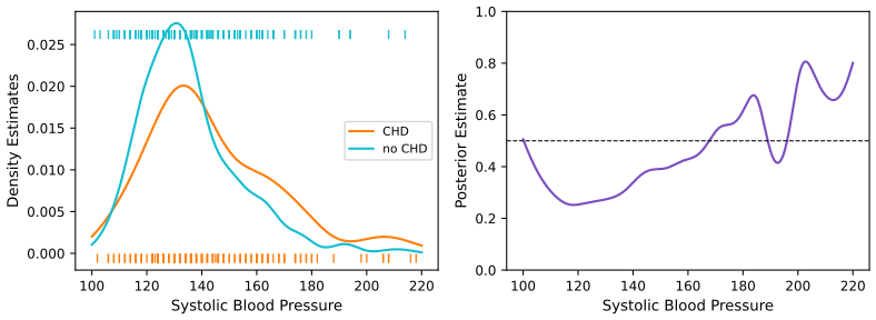
fig_6_14, kde_classifier. Reproduces Hastie, Tibshirani and Friedman (2009), Figure 6.14. Download: PDF · SVGIf classification is the goal, the class densities need not be estimated well everywhere: only the posterior near the decision boundary \(\{x:\Pr(G=1\given X=x)=\tfrac12\}\) matters. Figure 6.15 makes the point with two multimodal densities whose posterior is a plain logistic curve.
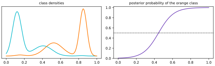
fig_6_15. Reproduces Hastie, Tibshirani and Friedman (2009), Figure 6.15. Download: PDF · SVG6.6.3 The Naive Bayes Classifier
pp. 210–211 When \(p\) is large, density estimation in \(\R^p\) is hopeless (Filling the gap 6.5). Naive Bayes assumes that, within each class, the features are independent:
\[ f_j(X)=\prod_{k=1}^pf_{jk}(X_k). \tag{6.26} \]Each marginal \(f_{jk}\) is then a one-dimensional estimate (a kernel density, a Gaussian, or a histogram for a discrete feature), which mixes variable types seamlessly.
Result 6.15 (naive Bayes has additive log-odds) p. 211, (6.27)
Under (6.26), with class \(J\) as the base,
\[ \log\frac{\Pr(G=\ell\given X)}{\Pr(G=J\given X)}=\log\frac{\pi_\ell f_\ell(X)}{\pi_Jf_J(X)}=\log\frac{\pi_\ell\prod_{k=1}^pf_{\ell k}(X_k)}{\pi_J\prod_{k=1}^pf_{Jk}(X_k)}=\log\frac{\pi_\ell}{\pi_J}+\sum_{k=1}^p\log\frac{f_{\ell k}(X_k)}{f_{Jk}(X_k)}=\alpha_\ell+\sum_{k=1}^pg_{\ell k}(X_k), \tag{6.27} \]which has the form of a generalised additive logistic model (Chapter 9).
Proof
Bayes' theorem gives \(\Pr(G=\ell\given X)=\pi_\ell f_\ell(X)/\sum_k\pi_kf_k(X)\); in the ratio of two classes the denominator cancels. Substitute (6.26), and use that the logarithm turns the product into a sum. Set \(\alpha_\ell=\log(\pi_\ell/\pi_J)\) and \(g_{\ell k}=\log(f_{\ell k}/f_{Jk})\). ∎
The two models are fitted differently (Exercise 6.9): naive Bayes estimates each \(f_{jk}\) from the class-\(j\) data alone (a generative, joint-likelihood fit), the additive logistic model maximises the conditional likelihood. The relation is that of linear discriminant analysis to logistic regression (Section 4.4.5 of the book). On the South African heart data with all nine predictors (famhist as a two-level histogram, the others with Silverman-bandwidth kernel densities), 10-fold cross-validation gives a misclassification rate of 33.3% for kernel naive Bayes against 28.4% for linear logistic regression; here the independence assumption costs more than the flexibility gains (code: naive_bayes_vs_logistic). The book's remark that naive Bayes "often" beats more sophisticated methods is about high-dimensional problems such as text, where the variance saved is large.
6.7 Radial Basis Functions and Kernels
pp. 212–214 Basis expansions (Chapter 5) fit \(f(x)=\sum_j\beta_jh_j(x)\) with fixed \(h_j\); kernel methods fit simple models locally. Radial basis functions combine the two by using kernels as basis functions:
\[ f(x)=\sum_{j=1}^MK_{\lambda_j}(\xi_j,x)\beta_j=\sum_{j=1}^MD\Big(\frac{\|x-\xi_j\|}{\lambda_j}\Big)\beta_j, \tag{6.28} \]with prototypes \(\xi_j\) and scales \(\lambda_j\). Fitting all parameters by least squares with Gaussian \(D\),
\[ \min_{\{\lambda_j,\xi_j,\beta_j\}_1^M}\ \sum_{i=1}^N\Big(y_i-\beta_0-\sum_{j=1}^M\beta_j\exp\Big\{-\frac{(x_i-\xi_j)^\T(x_i-\xi_j)}{\lambda_j^2}\Big\}\Big)^2, \tag{6.29} \]is an RBF network: nonconvex, with multiple local minima, fitted like a neural network. The simpler route chooses \(\{\lambda_j,\xi_j\}\) from the inputs alone (by clustering, or by a Gaussian mixture fitted to the \(x_i\)) and then the \(\beta_j\) by linear least squares; the drawback is that the response has no say in where the basis functions go. A common width \(\lambda_j=\lambda\) can leave holes, regions where no basis function is appreciably nonzero; the renormalised basis functions
\[ h_j(x)=\frac{D(\|x-\xi_j\|/\lambda)}{\sum_{k=1}^MD(\|x-\xi_k\|/\lambda)} \tag{6.30} \]sum to one everywhere and so cannot leave holes.
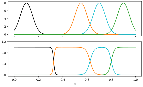
fig_6_16, rbf_basis. Reproduces Hastie, Tibshirani and Friedman (2009), Figure 6.16. Download: PDF · SVGResult 6.16 (Nadaraya–Watson as a renormalised RBF expansion) p. 213, (6.31)
The Nadaraya–Watson estimator in \(\R^p\) is an expansion in renormalised radial basis functions with one centre at each observation and coefficients equal to the responses:
\[ \hf(x_0)=\sum_{i=1}^Ny_i\frac{K_\lambda(x_0,x_i)}{\sum_{i=1}^NK_\lambda(x_0,x_i)}=\sum_{i=1}^Ny_ih_i(x_0), \tag{6.31} \]that is, \(\xi_i=x_i\) and \(\hat\beta_i=y_i\). By contrast, the kernel ridge regression solution (5.50) of Chapter 5, \(f(x)=\sum_i\hat\alpha_iK(x,x_i)\) with \(\hat\alpha=(\mathbf K+\lambda\mathbf I)^{-1}\by\), uses the unnormalised kernels with coefficients obtained by solving a linear system.
Proof
For a radial kernel, \(K_\lambda(x_0,x_i)=D(\|x_0-x_i\|/\lambda)\) is the basis function centred at \(\xi_i=x_i\) evaluated at \(x_0\); dividing by the sum over all centres is exactly (6.30) with \(M=N\). The fitted function is then linear in these basis functions with coefficients \(y_i\), with no fitting at all. ∎
Radial basis functions are the bridge between local fitting and the "kernel methods" of reproducing kernel Hilbert spaces: the same \(K\) appears either as a weight in a local fit or as a basis function in a penalised global fit.
See also (companion course): Section 6.3, radial basis function networks and Filling the gap 6.6 (normalised basis functions from an input-noise model).
6.8 Mixture Models for Density Estimation and Classification
pp. 214–216 The Gaussian mixture model
\[ f(x)=\sum_{m=1}^M\alpha_m\phi(x;\mu_m,\Sigma_m), \tag{6.32} \]with mixing proportions \(\alpha_m\ge0\), \(\sum_m\alpha_m=1\), is a flexible density estimate and a kind of kernel method. It is fitted by maximum likelihood with the EM algorithm (Chapter 8). If the covariances are scalar, \(\Sigma_m=\sigma_m^2\mathbf I\), (6.32) is a radial basis expansion. Fitted, it also gives the probability that observation \(i\) came from component \(m\),
\[ \hat r_{im}=\frac{\hat\alpha_m\phi(x_i;\hat\mu_m,\hat\Sigma_m)}{\sum_{k=1}^M\hat\alpha_k\phi(x_i;\hat\mu_k,\hat\Sigma_k)}. \tag{6.33} \]Filling the gap 6.9: EM for the one-dimensional mixture of Figure 6.17 p. 214
Derivation (sketch; full proofs in the companion course)
Introduce the unobserved component label \(Z_i\). If the labels were known, the complete-data log-likelihood \[\sum_i\sum_m\mathbf 1(Z_i=m)\{\log\alpha_m+\log\phi(x_i;\mu_m,\sigma_m^2)\}\] would be maximised by class proportions, class means and class variances. EM alternates: the E step replaces \(\mathbf 1(Z_i=m)\) by its conditional expectation given the data and the current parameters, which is the responsibility (6.33); the M step maximises the expected complete-data log-likelihood, giving \(N_m=\sum_i\hat r_{im}\), \(\hat\alpha_m=N_m/N\), \(\hat\mu_m=\sum_i\hat r_{im}x_i/N_m\), \(\hat\sigma_m^2=\sum_i\hat r_{im}(x_i-\hat\mu_m)^2/N_m\). Each iteration does not decrease the observed-data log-likelihood. The derivations of these updates, and the proof of monotonicity, are in the companion course, Section 9.2.2. ∎
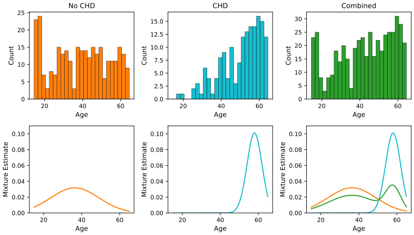
fig_6_17, em_gauss_1d. Reproduces Hastie, Tibshirani and Friedman (2009), Figure 6.17. Download: PDF · SVGThresholding the responsibility of the older component, \(\hat\delta_i=\mathbf 1(\hat r_{i2}>0.5)\), and cross-tabulating with CHD gives exactly the book's table:
| \(\hat\delta=0\) | \(\hat\delta=1\) | |
|---|---|---|
| CHD no | 232 | 70 |
| CHD yes | 76 | 84 |
The error rate is \((70+76)/462=31.6\%\); linear logistic regression of CHD on age, which does use the labels, misclassifies 32.0%.
Note on the book: a mixture with fixed widths does not tend to the kernel density estimate
The book states that if \(\Sigma_m=\sigma^2\mathbf I\) with \(\sigma\) fixed and \(M\uparrow N\), the maximum likelihood estimate of (6.32) approaches the kernel density estimate (6.22), with \(\hat\alpha_m=1/N\) and \(\hat\mu_m=x_m\). The kernel density estimate is one admissible value of the parameters, but in general it is not the maximum, and it is not even a fixed point of EM. Two points closer than \(2\sigma\) already show this: by the concavity of \(\phi_\sigma\) on \((-\sigma,\sigma)\), a single component at their midpoint gives each point the density \(\phi_\sigma(d/2)\ge\frac12\{\phi_\sigma(0)+\phi_\sigma(d)\}\), more than the two-component "kernel" fit. The maximum likelihood estimate with a fixed \(\sigma\) is the nonparametric maximum likelihood estimate of a mixing distribution (Lindsay, 1983), which typically has far fewer support points than \(N\). For the 160 blood pressures of Figure 6.13 with \(\sigma=7.55\): the kernel density estimate has log-likelihood \(-715.56\); EM started from it climbs to \(-711.59\), and the 160 means collapse onto 6 support points (116, 131, 141, 160, 173 and 207 mmHg). The statement becomes true only if \(\sigma\to0\) as well, or for data whose points are much farther apart than \(\sigma\). (Code: mixture_mle_fixed_sd.)
Separate mixtures within each class give flexible models for \(\Pr(G\given X)\) through Bayes' theorem; this is taken up in Chapter 12.
See also (companion course): Section 9.2, mixtures of Gaussians.
6.9 Computational Considerations
p. 216 Kernel and local regression and density estimation are memory-based: the whole training set is the model and all the work is done at prediction time, which can rule them out for real-time use. A fit at one point costs \(O(N)\) operations (unless the kernel is a box, whose sums can be updated as the window slides), against \(O(M)\) for an expansion in \(M\) basis functions, typically with \(M=O(\log N)\), after an initial \(O(NM^2+M^3)\) fit. Choosing \(\lambda\) by cross-validation costs \(O(N^2)\) (all \(N\) fits at all \(N\) points; Result 6.6 keeps it at one fit per \(\lambda\)). Software such as loess and locfit computes the fit exactly at \(M\) well-chosen vertices (\(O(NM)\)) and interpolates elsewhere (\(O(M)\) per point); kernel density estimates on a grid are computed by binning and the fast Fourier transform, since (6.23) is a convolution.
Bibliographic notes. p. 216 Loader (1999) covers local regression and likelihood and their software; Fan and Gijbels (1996) give the theory; Hastie and Tibshirani (1990) treat local regression within additive models; Silverman (1986) and Scott (1992) cover density estimation.
Exercises
All 12 exercises of Chapter 6 (Hastie, Tibshirani and Friedman, 2009, pp. 216–218), restated in my own words, with complete solutions (hidden).
Exercise 6.1. Show that the Nadaraya–Watson smoother with a fixed metric bandwidth and the Gaussian kernel is differentiable. What happens with the Epanechnikov kernel, and with the Epanechnikov kernel and an adaptive nearest-neighbour bandwidth?
Solution
Gaussian, fixed \(\lambda\). \(\hf(x)=A(x)/B(x)\) with \(A=\sum_i\phi((x-x_i)/\lambda)y_i\) and \(B=\sum_i\phi((x-x_i)/\lambda)\). Both are infinitely differentiable and \(B>0\) everywhere, so \(\hf\) is infinitely differentiable, with \(\hf'(x)=\sum_iK_i'(y_i-\hf(x))/\sum_iK_i\), \(K_i'=-\frac{x-x_i}{\lambda^2}K_i\).
Epanechnikov, fixed \(\lambda\). \(D\) is continuous and differentiable except at \(t=\pm1\), where its derivative jumps from \(\mp\tfrac32\) to 0. So \(A\) and \(B\) are continuous everywhere and differentiable except at the points \(x=x_i\pm\lambda\), where a data point enters or leaves the window. Where \(B>0\), \(\hf\) is continuous; it is differentiable except possibly at those finitely many points, where the one-sided derivatives differ by \(\frac{3}{2\lambda}(y_i-\hf(x))/B(x)\) in absolute value (nonzero unless \(y_i=\hf(x)\)). Where no point is within \(\lambda\), \(B=0\) and \(\hf\) is undefined. (The weight of an entering point grows linearly, not abruptly: that is why the fit is continuous, unlike the nearest-neighbour average.)
Epanechnikov, nearest-neighbour \(h(x)\). The \(k\)-th smallest of the continuous functions \(|x-x_i|\) is continuous and piecewise linear in \(x\), with kinks where two distances tie (midpoints between data points) or where \(x\) crosses a data point. Each weight \(D(|x-x_i|/h(x))\) is then continuous, and \(B(x)>0\) as long as at least one point is strictly inside the window (true when \(k\ge2\) and there are no ties). Hence \(\hf\) is continuous, but differentiable only piecewise: it has kinks at the points where \(h\) has kinks and where a point crosses the window's edge. (Note that the \(k\)-th neighbour always sits at the edge, with weight \(D(1)=0\).) A computation on the data of Figure 6.1 confirms that the fit has no jumps and that its derivative jumps at such points.
Exercise 6.2. Show that \(\sum_i(x_i-x_0)l_i(x_0)=0\) for local linear regression. With \(b_j(x_0)=\sum_i(x_i-x_0)^jl_i(x_0)\), show that \(b_0(x_0)=1\) for local polynomial regression of any degree (local constants included), and that \(b_j(x_0)=0\) for \(j=1,\dots,k\) for degree \(k\). What does this imply for the bias?
Solution
This is Result 6.4 (and Result 6.2 for \(k=1\), with an explicit formula). In the centred basis the equivalent kernel satisfies \(\bl(x_0)^\T\bB_0=\be_1^\T\); its entries are exactly \(b_0,b_1,\dots,b_k\). For the bias: Taylor-expanding \(f\) to order \(k\) with remainder, \[\E\hf(x_0)-f(x_0)=\sum_{j=k+1}^{\infty}\frac{f^{(j)}(x_0)}{j!}b_j(x_0)\] (or the Lagrange form of Result 6.4). Polynomials of degree at most \(k\) are reproduced exactly, and the bias depends only on derivatives of order \(k+1\) and higher; for local linear fits the leading term is \(\tfrac12f''(x_0)b_2(x_0)\), even at the boundary.
Exercise 6.3. Show that \(\|\bl(x)\|\) increases with the degree of the local polynomial.
Solution
As stated, this is false for general kernels: see the counterexample, where the squared norm drops from 0.4116 (degree 0) to 0.3400 (degree 1). What can be proved is Result 6.5: the equivalent kernel of degree \(d\) minimises \(\sum_il_i^2/K_i\) subject to the \(d+1\) moment conditions of Exercise 6.2, with minimum \(\be_1^\T(\bB_0^\T\bW\bB_0)^{-1}\be_1\). Adding a degree adds a constraint, so this weighted norm is nondecreasing. Consequences: (a) for the box (uniform) kernel, where the weights are equal on the window, \(\|\bl(x)\|\) itself is nondecreasing in the degree; (b) for any kernel, the variance under errors with \(\Var\varepsilon_i\propto1/K_i\) is nondecreasing; (c) asymptotically, in the interior the variances of degrees \(2\nu\) and \(2\nu+1\) agree to first order and the next even degree is strictly larger, while at the boundary each extra degree inflates the variance (Figure 6.6). With unequal weights the minimiser of the weighted norm need not minimise the plain norm, which is where the claim breaks.
Exercise 6.4. The \(p\) predictors are samples of smooth analogue curves at \(p\) equally spaced abscissae, with conditional covariance \(\Cov(X\given Y)=\Sigma\) roughly independent of \(Y\). Discuss the Mahalanobis choice \(\bA=\Sigma^{-1}\) in (6.14), compare it with \(\bA=\mathbf I\), and propose kernels that (a) downweight high-frequency components of the distance; (b) ignore them.
Solution
Let \(\Sigma=\sum_k d_kv_kv_k^\T\) with \(d_1\ge d_2\ge\cdots\). For smooth curves sampled on a grid, the eigenvectors \(v_k\) look like sinusoids of increasing frequency (they are close to the Fourier or Karhunen–Loève basis of the process) and the eigenvalues decay quickly: smooth curves have little variance in rapidly oscillating contrasts. Then
\[ (x-x_0)^\T\Sigma^{-1}(x-x_0)=\sum_k\frac{\{v_k^\T(x-x_0)\}^2}{d_k}. \]Mahalanobis. The weight \(1/d_k\) is largest for the highest frequencies, so the distance is dominated by the contrasts in which the curves hardly differ and in which measurement noise and discretisation error live. The metric amplifies noise, and \(\hat\Sigma^{-1}\) is badly estimated (the small eigenvalues are the least precisely estimated; with \(p\) close to \(N\) it may not exist). Euclidean \(\bA=\mathbf I\) gives every frequency weight one; the distance is dominated by the low-frequency components simply because they carry most of the variance, which is usually sensible, but noise in the high frequencies still adds to every distance. (a) Downweight high frequencies with \(\bA=\sum_kw_kv_kv_k^\T\), \(w_k\) decreasing in frequency, for example \(\bA=\Sigma\) itself, or \(\bA=\mathbf S^\T\mathbf S\) with \(\mathbf S\) a smoothing matrix (smooth each curve, then use Euclidean distance), or \(\bA=(\mathbf I+\gamma\boldsymbol\Omega)^{-1}\) with \(\boldsymbol\Omega=\mathbf{D}_2^\T\mathbf{D}_2\) a second-difference roughness matrix. (b) Ignore them with a rank-\(r\) projection, \(\bA=\sum_{k\le r}v_kv_k^\T\) (the leading principal components), or the projection \(\mathbf H(\mathbf H^\T\mathbf H)^{-1}\mathbf H^\T\) onto a low-dimensional smooth basis (natural splines with few knots, low-order Fourier terms). Since (6.14) only needs \(\bA\) positive semidefinite, singular choices are allowed; the kernel is then constant along the ignored directions (Filling the gap 6.6).
Exercise 6.5. Show that a locally constant multinomial logit model of the form (6.19) amounts to smoothing the indicator of each class separately with a Nadaraya–Watson smoother with weights \(K_\lambda(x_0,x_i)\).
Solution
This is Result 6.11: with intercepts only, (6.19) is \(\sum_jn_j\log p_j\) with \(n_j=\sum_iK_\lambda(x_0,x_i)\mathbf 1(g_i=j)\), maximised over the simplex at \(p_j=n_j/\sum_kn_k\), which is the Nadaraya–Watson average (6.2) of the responses \(\mathbf 1(g_i=j)\). The demonstration's local constant mode computes exactly this for two classes.
Exercise 6.6. You only have software for local regression in which you can choose exactly which monomials enter the fit. How would you fit a varying-coefficient model in some of the variables?
Solution
Let the model be \(f(x,z)=\alpha(z)+\sum_{j=1}^q\beta_j(z)x_j\). Run local regression on the joint inputs \((x,z)\) with two choices. (i) Make the kernel ignore \(x\): use a structured kernel (6.14) with \(\bA\) zero on the \(x\) coordinates (if the software only offers per-variable scale factors, give the \(x\) variables scale zero, equivalently an enormous bandwidth), so that \(K\) depends on \(z\) only. (ii) Choose the monomials \(1,x_1,\dots,x_q\): then at each target the local fit is \(\alpha+\sum_j\beta_jx_j\) with weights \(K_\lambda(z_0,z_i)\), which is (6.17). To make each coefficient locally linear in \(z\) (Result 6.9), add the monomials \(z\) and \(zx_1,\dots,zx_q\) (and not \(x_jx_k\) or \(x_j^2\)). The fitted surface at \((x,z_0)\) is linear in \(x\) for fixed \(z_0\), because neither the weights nor the local design depend on \(x_0\); so the coefficient functions can be read off from fitted values: \(\hat\alpha(z_0)=\hf(\mathbf 0,z_0)\) and \(\hat\beta_j(z_0)=\hf(\be_j,z_0)-\hf(\mathbf 0,z_0)\).
Exercise 6.7. Derive an expression for the leave-one-out cross-validated residual sum of squares for local polynomial regression.
Solution
Result 6.6: \(\mathrm{CV}=\frac1N\sum_i\{(y_i-\hf(x_i))/(1-S_{ii})\}^2\) with \(S_{ii}=l_i(x_i)\), so the residual sum of squares is \(\sum_i(y_i-\hf(x_i))^2/(1-S_{ii})^2\). It requires that the kernel weights of the other points do not change when \(x_i\) is deleted (true for metric windows). On the data of Figure 6.1 with the tri-cube kernel, \(\lambda=0.2\) and degree 1, the shortcut and \(N\) explicit refits agree to rounding error.
Exercise 6.8. Model the joint density of a continuous \((X,Y)\) with a bivariate Gaussian product kernel estimator, \(\phi_\lambda(X)\phi_\lambda(Y)\). Show that the conditional mean \(\E(Y\given X)\) of this estimate is a Nadaraya–Watson estimator. Extend this to classification with a continuous \(X\) and a discrete \(Y\).
Solution
\(\hf(x,y)=\frac1N\sum_i\phi_\lambda(x-x_i)\phi_\lambda(y-y_i)\). Then \(\int\hf(x,y)\d y=\frac1N\sum_i\phi_\lambda(x-x_i)\) and \(\int y\hf(x,y)\d y=\frac1N\sum_i\phi_\lambda(x-x_i)y_i\), because \(\int y\phi_\lambda(y-y_i)\d y=y_i\). Their ratio is \[\E(Y\given X=x)=\sum_i\phi_\lambda(x-x_i)y_i/\sum_i\phi_\lambda(x-x_i),\] the Gaussian Nadaraya–Watson estimator (6.2). (The \(y\)-bandwidth does not matter, and any kernel in \(y\) with mean zero works.) Classification: use the kernel \(\phi_\lambda(x-x_i)\,\mathbf 1(y=g_i)\) in the discrete coordinate. The estimate of \(\Pr(X\in\d x,Y=j)\) is \(\frac1N\sum_{i:g_i=j}\phi_\lambda(x-x_i)\d x\), and the conditional probability is \[\hat\Pr(Y=j\given x)=\sum_i\phi_\lambda(x-x_i)\mathbf 1(g_i=j)/\sum_i\phi_\lambda(x-x_i),\] which is (6.25) with a common bandwidth and sample proportions as priors (Result 6.14). A smoothed discrete kernel such as \((1-\epsilon)\) on \(y=g_i\) and \(\epsilon/(J-1)\) on the other classes (Aitchison and Aitken, 1976) shrinks the estimates towards \(1/J\). The continuous case is also derived in the companion course, Filling the gap 6.7.
Exercise 6.9. Compare the naive Bayes model (6.27) with a generalised additive logistic regression model in terms of (a) assumptions and (b) estimation. If all the \(X_k\) are discrete, what can you say about the corresponding GAM?
Solution
(a) Assumptions. Naive Bayes models the joint distribution: class priors and class-conditional densities that factorise over the features (6.26). That implies additive log-odds (Result 6.15) but is much stronger: many joint distributions with dependent features also have additive log-odds (for example any class-conditional dependence structure that is the same in all classes, \(f_j(x)=c(x)\prod_kf_{jk}(x_k)\), cancels in the ratio). The additive logistic model assumes only \(\logit\Pr(G=\ell\given X)=\alpha_\ell+\sum_kg_{\ell k}(X_k)\) and says nothing about the distribution of \(X\). (b) Estimation. Naive Bayes fits each \(f_{jk}\) separately from the class-\(j\) data (density estimation, no iteration, a joint likelihood); \(g_{\ell k}=\log(\hf_{\ell k}/\hf_{Jk})\) is inherited from the densities. The GAM maximises the conditional (multinomial) likelihood of \(G\) given \(X\) over the functions \(g_{\ell k}\), by backfitting within local scoring (Chapter 9). As with LDA versus logistic regression, naive Bayes is more efficient when its assumptions hold and can be badly biased (overconfident, because correlated features are counted twice) when they do not; the GAM is consistent under the weaker assumption. Discrete features. If every \(X_k\) is discrete, each \(g_{\ell k}\) is an arbitrary function on a finite set, i.e. a set of dummy-variable coefficients: the GAM is an ordinary multinomial logistic regression with main effects for every level of every feature. Naive Bayes produces one particular member of this family, \(g_{\ell k}(x_k)=\log\{\hat p_{\ell k}(x_k)/\hat p_{Jk}(x_k)\}\) from class-wise relative frequencies, whereas the logistic regression estimates the same coefficients by conditional maximum likelihood. On the heart data the naive Bayes classifier had a 10-fold CV error of 33.3% against 28.4% for linear logistic regression (Section 6.6.3).
Exercise 6.10. With \(y_i=f(x_i)+\varepsilon_i\), fixed \(x_i\), independent errors of mean zero and variance \(\sigma^2\), and a linear smoother \(\hat\bf=\bS_\lambda\by\), show that the average squared residual \(\ASR(\lambda)\) underestimates the in-sample prediction error (6.34), while \(C_\lambda\) of (6.35) is unbiased.
Solution
Result 6.7: \(\E\ASR=\PE-2\sigma^2\Tr(\bS_\lambda)/N\). For a local regression or a smoothing spline \(\Tr\bS_\lambda>0\) (the diagonal entries are leverages, nonnegative for these smoothers), so the training error is optimistic, and adding \(2\sigma^2\Tr(\bS_\lambda)/N\) removes the bias exactly. In practice \(\sigma^2\) is replaced by an estimate from a low-bias fit, e.g. \(\mathrm{RSS}/(N-2\Tr\bS+\Tr\bS^\T\bS)\) at a small \(\lambda\). A simulation with the design of Figure 6.1 confirms the identity.
Exercise 6.11. Show that for the Gaussian mixture model (6.32) the likelihood can be made arbitrarily large, and describe how.
Solution
Take \(M\ge2\). Put \(\mu_1=x_1\), \(\Sigma_1=\sigma^2\mathbf I\), \(\alpha_1=\alpha_2=\tfrac12\), and let the second component be any fixed Gaussian (say the sample mean and covariance), so that \(\phi(x_i;\mu_2,\Sigma_2)\ge c>0\) for all \(i\). Then the likelihood is at least
\[ \Big\{\tfrac12\phi(x_1;x_1,\sigma^2\mathbf I)\Big\}\prod_{i\ge2}\Big\{\tfrac12c\Big\}=\frac{1}{2(2\pi\sigma^2)^{p/2}}\Big(\frac c2\Big)^{N-1}\to\infty\quad(\sigma\to0). \]One component collapses onto a single observation with vanishing variance, while another component keeps the remaining likelihood terms bounded away from zero. This cannot happen with a single Gaussian, because then the other observations' densities go to zero faster. Remedies: bound the variances from below, constrain the covariances to be equal, use a prior (MAP), or look for a good local maximum and discard degenerate solutions. Full proof in the companion course: Result 9.3.
Exercise 6.12. Write a program for local linear discriminant analysis: at each query point \(x_0\) the training data get weights \(K_\lambda(x_0,x_i)\), and the ingredients of the linear discriminant functions (Section 4.3) are weighted averages. Run it on the zip-code data and report training and test errors for five values of \(\lambda\).
Solution
Method (
local_ldain the course code). For a query \(x_0\), Gaussian weights \(w_i=\exp\{-\|x_i-x_0\|^2/(2\lambda^2)\}\) on the 7291 training images (256 pixels); weighted class priors \(\hat\pi_k=\sum_{g_i=k}w_i/\sum_iw_i\), weighted class means \(\hat\mu_k\), and the weighted pooled within-class covariance \[\hat\Sigma=\sum_iw_i(x_i-\hat\mu_{g_i})(x_i-\hat\mu_{g_i})^\T/\sum_iw_i;\] then assign \(x_0\) to the class maximising \[\delta_k(x_0)=x_0^\T\hat\Sigma^{-1}\hat\mu_k-\tfrac12\hat\mu_k^\T\hat\Sigma^{-1}\hat\mu_k+\log\hat\pi_k\] (4.10). Two practical choices: the discriminant is computed in the space of the first 40 principal components of the training images (with narrow kernels a 256-dimensional weighted covariance is singular, and thousands of them are slow), with \(10^{-3}\) times the average eigenvalue added to the diagonal; classes with negligible weight are excluded. \(\lambda=\infty\) is ordinary LDA. The test error uses all 2007 test digits; the training error a fixed random subset of 1000 training digits.\(\lambda\) 4 6 8 12 \(\infty\) (LDA) training error 0.0% 1.6% 3.7% 5.9% 7.9% test error 4.8% 7.3% 8.9% 10.8% 12.7% The typical distance from a test image to its nearest training image is about 6.3 and to its 100th nearest about 10.5, so \(\lambda=4\) is very local: the query's own neighbourhood dominates, the training error is zero (each training point gets weight one at itself) and the test error is close to that of nearest-neighbour classification. As \(\lambda\) grows the fit becomes global LDA, whose linear boundaries are too rigid for the ten digit classes. Localising LDA buys a large improvement (12.7% to 4.8%).
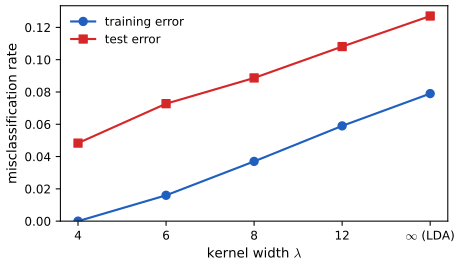
Figure 6.S2 (supplementary, Exercise 6.12). Training and test error of local linear discriminant analysis on the zip-code data. Code: fig_6_s2,local_lda_errors. Download: PDF · SVG
Demonstrations for this chapter
Each demonstration runs in the browser on the course's data files and links back to these notes. The ▶ Demo boxes above open them already set to the case under discussion.
| Demonstration | What you can see | Sections and results |
|---|---|---|
| Local regression at the boundary | Nadaraya–Watson, local linear and local quadratic fits with three kernels and metric or nearest-neighbour windows; the equivalent kernel at any target, its moments, the pointwise bias and standard deviation, \(\Tr\bS\) and leave-one-out CV. Presets: 1 N-W at the boundary; 2 local linear at the boundary; 3 curvature bias; 4 local quadratic; 5 quadratic variance at the edge. | 6.1.1, 6.1.2, 6.2; Results 6.2–6.6 |
| Bandwidth of a kernel density estimate | Gaussian KDEs of six heart-disease risk factors and of simulated two-peaked data; LSCV and likelihood-CV curves, Silverman's and the normal-reference rules, the exact ISE and MISE when the truth is known, and the effect of rounding. Presets: 1 Silverman (Fig 6.13); 2 LSCV collapse; 3 LSCV above the rounding unit; 4 two peaks; 5 small sample. | 6.6.1; Results 6.12, 6.13, Filling the gap 6.8 |
| Local logistic regression | Local constant and local linear logistic fits of CHD on six risk factors, with any span, the local model at any target on the probability and logit scales, sandwich bands, the kernel density classifier and global logistic regression. Presets: 1 SBP (Fig 6.12); 2 obesity; 3 local constant; 4 against the KDC (Fig 6.14); 5 age. | 6.5, 6.6.2; Results 6.10, 6.11, 6.14 |
Related demonstrations in the companion course: the density-estimation demo (histograms, kernels and nearest neighbours) and the Nadaraya–Watson preset of the kernel-functions demo. The Python code that produces every figure of this page is code/ch06_kernel_smoothing.py (see the code index).
References
- Hastie, T., Tibshirani, R. and Friedman, J. (2009). The Elements of Statistical Learning: Data Mining, Inference, and Prediction, 2nd edition. Springer, New York. Chapter 6, pp. 191–218. hastie.su.domains/ElemStatLearn.
- Aitchison, J. and Aitken, C. G. G. (1976). Multivariate binary discrimination by the kernel method. Biometrika, 63(3), 413–420.
- Bowman, A. W. (1984). An alternative method of cross-validation for the smoothing of density estimates. Biometrika, 71(2), 353–360.
- Buta, R. (1987). The structure and dynamics of ringed galaxies, III: surface photometry and kinematics of the ringed nonbarred spiral NGC 7531. The Astrophysical Journal Supplement Series, 64, 1–37.
- Cleveland, W. S. (1979). Robust locally weighted regression and smoothing scatterplots. Journal of the American Statistical Association, 74(368), 829–836.
- Epanechnikov, V. A. (1969). Non-parametric estimation of a multivariate probability density. Theory of Probability and Its Applications, 14(1), 153–158.
- Fan, J. and Gijbels, I. (1996). Local Polynomial Modelling and Its Applications. Chapman and Hall, London.
- Hastie, T. and Tibshirani, R. (1990). Generalized Additive Models. Chapman and Hall, London.
- Hastie, T. and Tibshirani, R. (1993). Varying-coefficient models. Journal of the Royal Statistical Society, Series B, 55(4), 757–796.
- Lindsay, B. G. (1983). The geometry of mixture likelihoods: a general theory. The Annals of Statistics, 11(1), 86–94.
- Loader, C. (1999). Local Regression and Likelihood. Springer, New York.
- Marron, J. S. and Wand, M. P. (1992). Exact mean integrated squared error. The Annals of Statistics, 20(2), 712–736.
- Nadaraya, E. A. (1964). On estimating regression. Theory of Probability and Its Applications, 9(1), 141–142.
- Parzen, E. (1962). On estimation of a probability density function and mode. The Annals of Mathematical Statistics, 33(3), 1065–1076.
- Rosenblatt, M. (1956). Remarks on some nonparametric estimates of a density function. The Annals of Mathematical Statistics, 27(3), 832–837.
- Rousseauw, J., du Plessis, J., Benade, A., Jordaan, P., Kotze, J., Jooste, P. and Ferreira, J. (1983). Coronary risk factor screening in three rural communities. South African Medical Journal, 64, 430–436.
- Rudemo, M. (1982). Empirical choice of histograms and kernel density estimators. Scandinavian Journal of Statistics, 9(2), 65–78.
- Scott, D. W. (1992). Multivariate Density Estimation: Theory, Practice, and Visualization. Wiley, New York.
- Silverman, B. W. (1986). Density Estimation for Statistics and Data Analysis. Chapman and Hall, London.
- Tibshirani, R. and Hastie, T. (1987). Local likelihood estimation. Journal of the American Statistical Association, 82(398), 559–567.
- Wand, M. P. and Jones, M. C. (1995). Kernel Smoothing. Chapman and Hall, London.
- Watson, G. S. (1964). Smooth regression analysis. Sankhyā, Series A, 26(4), 359–372.
The numerical statements in the text (kernel constants, the moment identities of the equivalent kernels, the boundary constants, the leave-one-out shortcut, the unbiasedness of \(C_p\) and of LSCV, the tied-data limit of LSCV, the mixture fit of Figure 6.17 and the corrections to Exercise 6.3 and Section 6.8) were confirmed numerically.