Deep Learning
A neural network builds its own features: each hidden unit takes a linear combination of the inputs and bends it through a fixed nonlinearity, and the output is an ordinary linear (or logistic, or multinomial) model in these learned features. Stacking such layers, sharing weights across the positions of an image (convolutional networks) or across the steps of a sequence (recurrent networks), and fitting millions of parameters by stochastic gradient descent with heavy regularisation gives the methods called deep learning. This chapter explains the models and how they are fitted, and asks when they are worth it: on 263 baseball players a linear model does as well, on 60,000 handwritten digits a network is far better. It ends with double descent, the surprising good behaviour of models that interpolate the training data.
Ch. 1 Introduction Ch. 2 Statistical learning Ch. 3 Linear regression Ch. 4 Classification Ch. 5 Resampling Ch. 6 Selection and regularization Ch. 7 Beyond linearity Ch. 8 Trees Ch. 9 SVMs Ch. 10 Deep learning Ch. 11 Survival analysis Ch. 12 Unsupervised learning Ch. 13 Multiple testing
How to read these notes
They follow the book. Sections carry the book's numbers (10.1, 10.3.2, ...), and displayed equations that appear in the book carry its equation numbers, e.g. \((10.13)\); equations without a number are steps the book skips. Page numbers refer to the R edition (2021); the Python edition (2023) has the same text, figures and exercises a few pages later.
Filling the gaps. The book says of Section 10.7 that readers "can safely skip it". Here the missing steps are written out at the level of a first course in calculus and regression: the parameter counts, the softmax likelihood, convolution as a constrained linear layer, backpropagation by the chain rule, why gradient descent goes downhill, why dropout and data augmentation act like ridge regression, and what the minimum-norm solution is. Each is in an orange Filling the gap box; derivations start hidden. Green Deeper lines point to the graduate course on the same authors' larger book.
The lab in two languages. Section 10.9 shows each step in R (left) and Python (right). The book's R lab needs keras and a Python installation of TensorFlow; here the R networks are written out in base R (forward pass, backpropagation, dropout and RMSprop in about sixty lines), which runs anywhere and shows every step of Section 10.7. The Python lab uses plain PyTorch. The convolutional network is in Python only, and the pretrained ResNet50 and the IMDb models, which need large downloads, are described but not run (see where the two languages differ).
Main reference
G. James, D. Witten, T. Hastie and R. Tibshirani, An Introduction to Statistical Learning with Applications in R, 2nd edition, Springer (2021), Chapter 10, pages 403–460, and G. James, D. Witten, T. Hastie, R. Tibshirani and J. Taylor, An Introduction to Statistical Learning with Applications in Python, Springer (2023), Chapter 10 (book website, with the data and the labs: www.statlearning.com). Section, equation, figure and exercise numbers below refer to these books.
The explanations, derivations, figures and code are my own; equations are cited by their numbers in the book.
Companion courses
- Statistical Learning: Theory and Methods (Hastie, Tibshirani and Friedman 2009), the graduate version of this chapter: Chapter 11, Neural Networks (projection pursuit, back-propagation, weight decay, the ZIP code networks with local connectivity and shared weights). Each section below links to the matching part.
- Foundations of Deep Learning (Bishop and Bishop 2024), which goes much further: Chapter 6 (deep networks and error functions), Chapter 7 (gradient descent, minibatches, RMSProp and Adam), Chapter 8 (backpropagation and automatic differentiation), Chapter 9 (weight decay, early stopping, double descent, dropout), Chapter 10 (convolutional networks) and Chapter 12 (word embeddings, recurrent networks and transformers).
- Bayesian and Probabilistic Machine Learning (Bishop 2006): Chapter 5, Neural Networks, the same models seen from the likelihood side.
The chapter at a glance
- 10.1–10.2 A network with one hidden layer is a linear model in \(K\) learned features \(A_k=g(w_{k0}+\sum_jw_{kj}X_j)\). The nonlinearity \(g\) is essential: without it the model collapses to a linear one (Result 10.1). The MNIST network of Figure 10.4 has 235,146 parameters (Filling the gap 10.2), and its softmax output with cross-entropy is multinomial logistic regression on the last hidden layer (Filling the gap 10.3).
- 10.3 A convolution layer is a dense layer with mostly zero, shared weights (Filling the gap 10.4); max pooling buys some location invariance. The CIFAR100 network has 964,516 parameters, 54% of them in one dense layer. Data augmentation acts like a ridge penalty (Filling the gap 10.5).
- 10.4–10.5 Bag-of-words features make a document a long sparse binary vector; a two-class network is a nonlinear logistic regression (Result 10.4). A recurrent network applies the same weights at every step of a sequence; with a linear activation it is an autoregressive model with structured coefficients (Filling the gap 10.7). On the NYSE volume series it does as well as AR(5), test \(R^2\approx0.41\).
- 10.6 On the Hitters data a 1409-parameter network does no better than least squares and the lasso (Table 10.2, recomputed).
- 10.7 Backpropagation is the chain rule, bookkept layer by layer (Filling the gap 10.9). Gradient descent decreases the objective for a small enough step, and a minibatch gradient is unbiased (Filling the gap 10.10). Dropout is unbiased and, for a linear model, exactly a data-dependent ridge penalty (Filling the gap 10.11).
- 10.8 Past the interpolation threshold the minimum-norm solution \(\bB^\T(\bB\bB^\T)^{-1}\by\) is selected; it is the limit of ridge regression and where gradient descent from zero ends (Filling the gap 10.12), and its test error falls again: double descent.
Notation. Inputs \(X=(X_1,\dots,X_p)\); observations \((x_i,y_i)\), \(i=1,\dots,n\). \(g\) is the activation function, \((z)_+=\max(z,0)\). In a layer with \(K\) units, unit \(k\) computes \(z_k=w_{k0}+\sum_jw_{kj}x_j\) and \(A_k=g(z_k)\). All the parameters together form one long vector \(\bth\).
Prerequisites. Linear and logistic regression (Chapters 3 and 4), multinomial logistic regression (Section 4.3.5), the validation set (Section 5.1.1), ridge and the lasso (Section 6.2), natural splines (Section 7.4).
pp. 403–404 Neural networks rose to fame in the late 1980s, fell out of favour when support vector machines, boosting and random forests proved easier to use, and came back after 2010 as deep learning, with new architectures and very large training sets. The chapter covers the basic network, then two specialisations: convolutional networks for images and recurrent networks for sequences.
10.1 Single Layer Neural Networks
Definition 10.1 (feed-forward network with one hidden layer) pp. 404–405, (10.1)–(10.3), Figure 10.1
Given inputs \(X=(X_1,\dots,X_p)\), a network with \(K\) hidden units predicts a quantitative response by
\[ f(X)=\beta_0+\sum_{k=1}^K\beta_kh_k(X)=\beta_0+\sum_{k=1}^K\beta_k\,g\Big(w_{k0}+\sum_{j=1}^pw_{kj}X_j\Big). \tag{10.1} \]It is built in two steps. The hidden layer computes the activations
\[ A_k=h_k(X)=g\Big(w_{k0}+\sum_{j=1}^pw_{kj}X_j\Big),\qquad k=1,\dots,K, \tag{10.2} \]with an activation function \(g\) fixed in advance, and the output layer is a linear regression on them,
\[ f(X)=\beta_0+\sum_{k=1}^K\beta_kA_k. \tag{10.3} \]All of \(\beta_0,\dots,\beta_K\) and \(w_{10},\dots,w_{Kp}\) are estimated from the data: \(K(p+1)+K+1\) parameters. The \(A_k\) are like the basis functions of Chapter 7, except that they are learned rather than fixed. In machine-learning language the coefficients are weights and the intercepts \(w_{k0}\), \(\beta_0\) are biases (not to be confused with the bias of the bias-variance trade-off).
Definition 10.2 (sigmoid and ReLU activations) p. 405, (10.4)–(10.5), Figure 10.2
\[ g(z)=\frac{e^z}{1+e^z}=\frac1{1+e^{-z}}\quad\text{(sigmoid)}, \tag{10.4} \] \[ g(z)=(z)_+=\begin{cases}0 & z\lt0\\ z & \text{otherwise}\end{cases}\quad\text{(rectified linear unit, ReLU)}. \tag{10.5} \]The sigmoid is the function of logistic regression; it was the early favourite. The ReLU is the modern default: it is cheap to compute and to differentiate, and the intercept \(w_{k0}\) moves its kink to wherever the data need it.
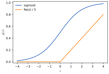
fig_10_2. Reproduces James et al. (2021), Figure 10.2. Download: PDF · SVGResult 10.1 (the nonlinearity is essential, and it creates interactions) p. 406, (10.6)–(10.8)
(a) If \(g\) is linear, \(g(z)=a+bz\), then (10.1) is a linear function of \(X\): the network is just a linear regression, however many hidden units it has. (b) With \(p=2\), \(K=2\), \(g(z)=z^2\) and
\[ \beta_0=0,\ \beta_1=\tfrac14,\ \beta_2=-\tfrac14,\quad w_{10}=0,\ w_{11}=1,\ w_{12}=1,\quad w_{20}=0,\ w_{21}=1,\ w_{22}=-1, \tag{10.6} \]the hidden units are
\[ h_1(X)=(0+X_1+X_2)^2,\qquad h_2(X)=(0+X_1-X_2)^2, \tag{10.7} \]and the network computes the interaction
\[ f(X)=\tfrac14\big[(X_1+X_2)^2-(X_1-X_2)^2\big]=X_1X_2. \tag{10.8} \]Filling the gap 10.1: why a linear \(g\) collapses the network, and why sums of bent linear functions are so flexible p. 406
Derivation
(a) With \(g(z)=a+bz\), each \(A_k=a+b\,w_{k0}+\sum_jb\,w_{kj}X_j\) is a linear function of \(X\), and (10.3) adds them up with weights:
\[ f(X)=\Big(\beta_0+\sum_k\beta_k(a+bw_{k0})\Big)+\sum_{j=1}^p\Big(\sum_k\beta_kbw_{kj}\Big)X_j=\gamma_0+\sum_j\gamma_jX_j. \]A composition of linear maps is linear, so stacking more linear layers changes nothing either. All the flexibility of a network comes from the nonlinearity of \(g\).
(b) Expand:
\[ (X_1+X_2)^2-(X_1-X_2)^2=(X_1^2+2X_1X_2+X_2^2)-(X_1^2-2X_1X_2+X_2^2)=4X_1X_2. \]The identity \(uv=\frac14[(u+v)^2-(u-v)^2]\) (the polarisation identity) shows more: any product of two linear combinations of the inputs is a sum of two squared linear combinations, so with \(g(z)=z^2\) a network can represent every quadratic polynomial in \(X\) (but nothing of higher degree: a sum of squares of linear functions is a quadratic).
Why sigmoids and ReLUs have no such limit. A sum \(\sum_k\beta_k(w_{k0}+w_kX)_+\) of ReLUs of one input is a continuous piecewise-linear function with a kink at each \(-w_{k0}/w_k\); with enough units it can follow any continuous function on an interval as closely as we like (join the dots of the function at fine spacing). In several inputs, sums of functions of linear combinations (ridge functions) can approximate any continuous function on a bounded set: this is the universal approximation property of one-hidden-layer networks (Cybenko 1989; Hornik, Stinchcombe and White 1989). The catch is in "enough units"; Section 10.2 explains why depth helps in practice.
Deeper: Statistical Learning: Theory and Methods, Result 11.1 (products are sums of ridge functions) and Result 11.4 (universal approximation by one hidden layer); a network is projection pursuit regression with sigmoidal ridge functions, Result 11.3. See also: activation functions and their derivatives and the linear regions of a ReLU network in Foundations of Deep Learning.
p. 406 For a quantitative response the parameters are chosen to minimise the squared error
\[ \sum_{i=1}^n\big(y_i-f(x_i)\big)^2, \tag{10.9} \]which, because \(f\) depends on the \(w_{kj}\) through \(g\), is a nonlinear least-squares problem; Section 10.7 explains how it is solved.
10.2 Multilayer Neural Networks
pp. 407–408 A single hidden layer with many units can approximate most functions, but finding a good fit is much easier with several layers of moderate size. The example is the MNIST digits (LeCun, Cortes and Burges 2010): 28 × 28 grey-scale images, so \(p=784\) inputs with values from 0 to 255, ten classes 0–9, 60,000 training and 10,000 test images. The response is coded by ten dummy variables \(Y=(Y_0,\dots,Y_9)\) (one-hot encoding).
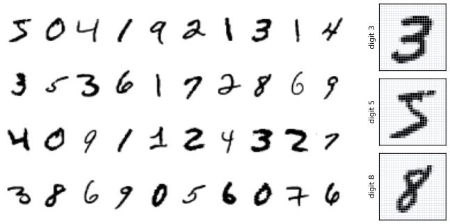
fig_10_3, data from common.mnist. Reproduces James et al. (2021), Figure 10.3. Download: PDF · SVGDefinition 10.3 (a network with two hidden layers and ten outputs) pp. 408–409, (10.10)–(10.12), Figure 10.4
The first hidden layer \(L_1\) has \(K_1=256\) units and the second \(L_2\) has \(K_2=128\):
\[ A^{(1)}_k=h^{(1)}_k(X)=g\Big(w^{(1)}_{k0}+\sum_{j=1}^pw^{(1)}_{kj}X_j\Big),\qquad k=1,\dots,K_1, \tag{10.10} \] \[ A^{(2)}_\ell=h^{(2)}_\ell(X)=g\Big(w^{(2)}_{\ell0}+\sum_{k=1}^{K_1}w^{(2)}_{\ell k}A^{(1)}_k\Big),\qquad \ell=1,\dots,K_2. \tag{10.11} \]Each \(A^{(2)}_\ell\) is still a function of \(X\), through a chain of transformations. The output layer computes ten linear combinations of the second-layer activations,
\[ Z_m=\beta_{m0}+\sum_{\ell=1}^{K_2}\beta_{m\ell}h^{(2)}_\ell(X)=\beta_{m0}+\sum_{\ell=1}^{K_2}\beta_{m\ell}A^{(2)}_\ell,\qquad m=0,1,\dots,9. \tag{10.12} \]The weight matrices are \(\bW_1\) (785 × 256, the extra row for the biases), \(\bW_2\) (257 × 128) and \(\bB\) (129 × 10).
Filling the gap 10.2: counting the parameters of a dense network pp. 408–410, Figure 10.4 and Table 10.2
Derivation
A dense (fully connected) layer from \(a\) inputs to \(b\) units has one weight for each input-unit pair and one bias per unit: \(ab+b=(a+1)b\) parameters. A network with layer sizes \(K_0=p,K_1,\dots,K_L\) therefore has \(\sum_{l=1}^L(K_{l-1}+1)K_l\) parameters. For Figure 10.4:
\[ (784+1)\cdot256+(256+1)\cdot128+(128+1)\cdot10=200{,}960+32{,}896+1{,}290=235{,}146. \]Multinomial logistic regression is the network with no hidden layer: \((784+1)\cdot10=7{,}850\) parameters, or \(785\times9=7{,}065\) after removing the redundant class (see Filling the gap 10.3); \(235{,}146/7{,}065=33.3\), the book's "more than 33 times". With 60,000 training images there are \(235{,}146/60{,}000=3.9\) parameters per observation, hence the need for regularisation.
The Hitters network of Table 10.2. One hidden layer of 64 units on \(p\) inputs has \(64(p+1)+65\) parameters. The book's 1,409 corresponds to \(p=20\): \(64\cdot21+65=1{,}409\). With the 19 predictors of the Hitters data one would expect \(p=19\) and 1,345. The 20 comes from R's model.matrix(Salary ~ . - 1): without an intercept the first factor, League, gets a dummy for both of its levels (LeagueA and LeagueN), so the 16 numeric columns and four dummies make 20. The Python edition's model matrix has 19 columns, and its lab network of 50 units has \(50\cdot19+50+50+1=1{,}051\) parameters; with R's 20 columns it is 1,101, as in both labs here.
Definition 10.4 (softmax output and cross-entropy) p. 410, (10.13)–(10.14)
To turn the ten \(Z_m\) into class probabilities, the output layer applies the softmax (as in (4.13)):
\[ f_m(X)=\Pr(Y=m\given X)=\frac{e^{Z_m}}{\sum_{\ell=0}^9e^{Z_\ell}},\qquad m=0,1,\dots,9. \tag{10.13} \]The fit minimises the negative multinomial log-likelihood, also called the cross-entropy,
\[ -\sum_{i=1}^n\sum_{m=0}^9y_{im}\log\big(f_m(x_i)\big). \tag{10.14} \]The classifier assigns an image to the class with the largest \(f_m\).
Filling the gap 10.3: why (10.14) is the negative log-likelihood, why softmax is over-parametrised, and the derivative that drives backpropagation p. 410; Exercises 2 and 3
Derivation
Likelihood. Given \(x_i\), the class is one draw from the ten probabilities \(f_0(x_i),\dots,f_9(x_i)\). The probability of the observed class is \(\prod_mf_m(x_i)^{y_{im}}\), because exactly one \(y_{im}\) equals 1. For independent observations the likelihood is \(\prod_i\prod_mf_m(x_i)^{y_{im}}\), and minus its logarithm is (10.14). With two classes, \(y_{i1}=y_i\), \(y_{i0}=1-y_i\) and \(f_1=p(x_i)\), it is
\[ -\sum_i\big[y_i\log p(x_i)+(1-y_i)\log(1-p(x_i))\big], \]minus the log of the logistic likelihood (4.5) (Exercise 3).
Over-parametrisation. Adding the same constant \(c\) to every \(Z_\ell\) multiplies numerator and denominator of (10.13) by \(e^c\), so the probabilities do not change (Exercise 2). Hence only differences \(Z_m-Z_0\) matter, and one class's coefficients can be fixed at zero, as in Section 4.3.5. Software keeps all ten and lets regularisation or SGD pick one of the equivalent solutions.
The derivative. For one observation the loss is \(R_i=-\sum_my_{im}\log f_m\), with
\[ \log f_m=Z_m-\log\sum_\ell e^{Z_\ell}, \]so that
\[ \frac{\partial R_i}{\partial Z_m}=-y_{im}+\sum_\ell y_{i\ell}\frac{e^{Z_m}}{\sum_ke^{Z_k}}=f_m(x_i)-y_{im}, \]using \(\sum_\ell y_{i\ell}=1\). The derivative of the cross-entropy with respect to the logits is "predicted probability minus indicator", just as the derivative of \(\frac12(y-f)^2\) with respect to \(f\) is minus the residual. This is the quantity softmax(out) - y that the R lab's fit_mlp passes back through the network.
Deeper: Statistical Learning: Theory and Methods, Result 11.6 (softmax outputs with cross-entropy). See also: error functions as negative log-likelihoods in Foundations of Deep Learning, and multinomial logistic regression in Chapter 4, Section 4.3.5.
pp. 410–411 Table 10.1 compares the network with two linear classifiers of Chapter 4. Our recomputation (same architecture; details in the code's docstring) agrees with the book to a few tenths of a percent, and LDA's 12.7% exactly.
| Method | Test error, book | Test error, here |
|---|---|---|
| Neural network + ridge regularisation | 2.3% | 1.7% |
| Neural network + dropout regularisation | 1.8% | 1.8% |
| Multinomial logistic regression | 7.2% | 7.5% |
| Linear discriminant analysis | 12.7% | 12.7% |
Table 10.1, recomputed: the network of Figure 10.4 trained for 30 epochs by RMSprop on 48,000 images (the other 12,000 are the validation set); the ridge penalty \(\lambda\) of (10.31) was chosen on the validation set. In our run ridge did slightly better than dropout; with other settings the order changes, which is the book's point in Section 10.7.4 about tuning.
10.3 Convolutional Neural Networks
pp. 411–412 Convolutional neural networks (CNNs) drove the return of neural networks around 2010. The example data set, CIFAR100, has 60,000 colour images of 32 × 32 pixels in 100 classes; each image is a three-dimensional array, a feature map, with two spatial axes and a channel axis for red, green and blue. A CNN first finds low-level features (edges, patches of colour), then combines them into higher-level ones (an eye, an ear), and finally into a class. It does this with two special kinds of hidden layer: convolution layers and pooling layers. (The CIFAR100 images of Figure 10.5 and the cartoon of Figure 10.6 are not reproduced; the images are a 160 MB download that this course does not need.)
10.3.1 Convolution Layers
Definition 10.5 (convolution filter) pp. 412–413
A convolution filter is a small array of weights, say \(\ell_1\times\ell_2\). Convolving an image with it means placing the filter on every \(\ell_1\times\ell_2\) patch of the image, multiplying elementwise and adding up. For a 4 × 3 image and a 2 × 2 filter,
\[ \begin{bmatrix}a&b&c\\d&e&f\\g&h&i\\j&k&l\end{bmatrix}\ \text{and}\ \begin{bmatrix}\alpha&\beta\\\gamma&\delta\end{bmatrix}\ \text{give}\ \begin{bmatrix}a\alpha+b\beta+d\gamma+e\delta & b\alpha+c\beta+e\gamma+f\delta\\ d\alpha+e\beta+g\gamma+h\delta & e\alpha+f\beta+h\gamma+i\delta\\ g\alpha+h\beta+j\gamma+k\delta & h\alpha+i\beta+k\gamma+l\delta\end{bmatrix}. \]In symbols,
\[ \text{out}_{rs}=\sum_{a=1}^{\ell_1}\sum_{b=1}^{\ell_2}\text{image}_{r+a-1,\,s+b-1}\,\text{filter}_{ab}. \]The output is large where the patch resembles the filter, so the convolved image highlights the places where the filter's pattern occurs. Without padding an \(H\times W\) image gives an \((H-\ell_1+1)\times(W-\ell_2+1)\) output; adding \((\ell-1)/2\) rows and columns of zeros around the image (padding, "same" in software) keeps the size.
A convolution layer uses a bank of \(K\) filters, learned from the data. On a \(C\)-channel input each filter has \(C\) channels; the \(C\) convolutions are added, a bias is added and the ReLU is applied (the detector layer), giving one output channel per filter: a \(K\)-channel feature map.
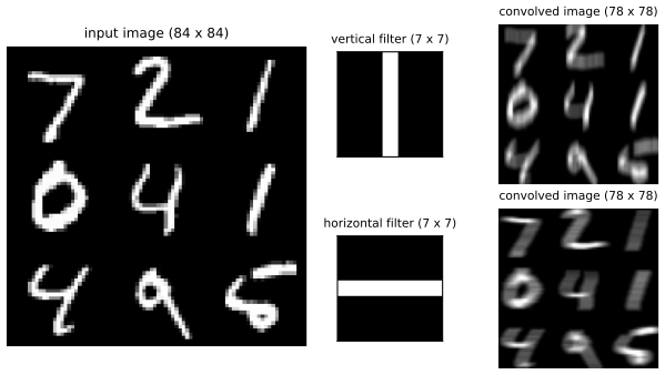
fig_10_7, conv2d_valid. Reproduces James et al. (2021), Figure 10.7. Download: PDF · SVGFilling the gap 10.4: a convolution layer is a dense layer with shared, mostly zero weights, and its parameter count p. 414, "see Exercise 4"; pp. 450–451
Derivation
As a constrained dense layer. Stack the pixels of a one-channel \(H\times W\) image into a vector \(x\) of length \(HW\), and the convolved image into a vector \(u\). Each output \(u_{rs}\) is a linear combination of the pixels, \(u_{rs}=\sum_{q}M_{(rs),q}x_q\), so the convolution is a matrix product \(u=Mx\), the same operation as a dense layer (before the bias and activation). But \(M\) is very special: the row for output \((r,s)\) is zero except on the \(\ell_1\ell_2\) pixels of the patch at \((r,s)\) (structural zeros), and these nonzero entries are the same filter weights in every row (weight sharing, the old name in the book's footnote 10). A dense layer with as many hidden units would have \(HW\) free weights per unit; the convolution has \(\ell_1\ell_2\) weights for all of them.
Counting. A layer of \(K\) filters of size \(\ell\times\ell\) on a \(C\)-channel input has \(K(\ell^2C+1)\) parameters, whatever the size of the image. For the CIFAR100 network of the lab (3 × 3 filters, padding "same", each followed by 2 × 2 max pooling):
| Layer | Output | Parameters |
|---|---|---|
| convolution, 32 filters on 3 channels | 32 × 32 × 32 | \(32(9\cdot3+1)=896\) |
| convolution, 64 filters on 32 channels | 16 × 16 × 64 | \(64(9\cdot32+1)=18{,}496\) |
| convolution, 128 filters on 64 channels | 8 × 8 × 128 | \(128(9\cdot64+1)=73{,}856\) |
| convolution, 256 filters on 128 channels | 4 × 4 × 256 | \(256(9\cdot128+1)=295{,}168\) |
| flatten 2 × 2 × 256, dense to 512 | 512 | \((1024+1)\cdot512=524{,}800\) |
| dense to 100 classes | 100 | \((512+1)\cdot100=51{,}300\) |
| total | 964,516 |
(Each pooling layer halves the two spatial sizes and has no parameters.) More than half of the parameters sit in the single dense layer after flattening. A dense layer producing the first feature map from the raw image would need \((32\cdot32\cdot3+1)\cdot(32\cdot32\cdot32)\approx10^8\) parameters instead of 896. The Python lab builds this network and confirms the count. Gradients of shared weights are sums over the positions where they are used.
Deeper: Statistical Learning: Theory and Methods, Section 11.7 (the ZIP code networks: local connectivity and shared weights, the ancestors of CNNs) and Result 11.12 (the gradient of a shared weight). See also: a convolutional layer as a sparse, weight-shared layer, the size of a feature map and translation equivariance in Foundations of Deep Learning, with its convolution arithmetic demonstration.
10.3.2 Pooling Layers
Definition 10.6 (max pooling) p. 415
A max pooling layer replaces each non-overlapping 2 × 2 block of a feature map by its largest value, halving both spatial sizes:
\[ \begin{bmatrix}1&2&5&3\\3&0&1&2\\2&1&3&4\\1&1&2&0\end{bmatrix}\ \longrightarrow\ \begin{bmatrix}3&5\\2&4\end{bmatrix}. \]It has no parameters, and it gives some location invariance: as long as one of the four pixels of a block is large, the block registers as large, wherever in the block the feature sits.
p. 415 Convolution is equivariant: shift the image and the convolved image shifts with it. Pooling turns this into approximate invariance: a shift of one pixel moves a feature within its 2 × 2 block half of the time, and then the pooled value does not change at all; two rounds of pooling tolerate larger shifts. On a digit shifted by one pixel the convolved maps of the demonstration below correlate poorly, position by position, with those of the unshifted digit, while the maps after two rounds of pooling nearly coincide.
See also: what pooling buys, exactly and approximately (Foundations of Deep Learning, Filling the gap 10.8).
10.3.3 Architecture of a Convolutional Neural Network
pp. 415–417, Figure 10.8 A CNN for CIFAR100 alternates convolution and pooling: the 32 × 32 × 3 input becomes 32 × 32 × \(K_1\) after the first convolution (with padding), 16 × 16 × \(K_1\) after pooling, and so on. Because each pooling shrinks the maps, the number of filters is usually increased in the next layer. When the maps are only a few pixels wide they are flattened (each pixel of each channel becomes a separate unit) and fed to one or more dense layers and a softmax over the 100 classes. The parameters are the filter weights; the count for the lab's network is in Filling the gap 10.4. Dropout and ridge or lasso penalties can be used at every layer.
10.3.4 Data Augmentation
p. 417, Figure 10.9 Each training image is replicated many times with small natural distortions (zoom, shifts, shear, small rotations, and for natural images horizontal flips) that do not change its label. In stochastic gradient descent the distortions can be drawn afresh for every minibatch, so nothing needs to be stored. The book likens this "fattening" of the data to ridge regularisation; the next box makes the analogy exact in the simplest case.

fig_10_9, augment. Reproduces James et al. (2021), Figure 10.9. Download: PDF · SVGFilling the gap 10.5: adding noise to the inputs is ridge regression p. 417, "similar in spirit to ridge regularization"
Derivation
Take a linear model \(f(x)=\beta_0+x^\T\beta\) and replace every training input \(x_i\) by a randomly perturbed copy \(x_i+\varepsilon_i\), with \(\varepsilon_i\) independent of everything, mean zero and covariance \(\sigma^2\bI\). The expected squared error over the perturbations is
\[ \E\sum_i\big(y_i-\beta_0-(x_i+\varepsilon_i)^\T\beta\big)^2=\sum_i\big(y_i-\beta_0-x_i^\T\beta\big)^2-2\sum_i(y_i-\beta_0-x_i^\T\beta)\,\E[\varepsilon_i]^\T\beta+\sum_i\E\big[(\varepsilon_i^\T\beta)^2\big]. \]The middle term vanishes because \(\E\varepsilon_i=0\), and \(\E[(\varepsilon_i^\T\beta)^2]=\beta^\T\E[\varepsilon_i\varepsilon_i^\T]\beta=\sigma^2\|\beta\|^2\). Hence
\[ \E\sum_i\big(y_i-\beta_0-(x_i+\varepsilon_i)^\T\beta\big)^2=\sum_i\big(y_i-\beta_0-x_i^\T\beta\big)^2+n\sigma^2\sum_j\beta_j^2, \]the ridge criterion (6.5) with \(\lambda=n\sigma^2\): training on a cloud of noisy copies around each point shrinks the coefficients exactly as ridge does (Bishop 1995). Image distortions are not isotropic noise, so for a CNN the correspondence is only approximate: augmentation penalises sensitivity of the fit along the directions of the distortions (small rotations, shifts), which is the kind of invariance we want.
See also: augmentation with small transformations is tangent propagation; noise is Tikhonov regularisation (Foundations of Deep Learning, Filling the gap 9.2), and ridge regression in Chapter 6, Section 6.2.1.
10.3.5 Results Using a Pretrained Classifier
pp. 417–419, Figure 10.10 The resnet50 classifier (He et al. 2016), a 50-layer CNN trained on the imagenet database of millions of images, is applied to six photographs from one of the authors' albums. It is confident about the flamingo, reasonable about a hawk seen close up, and confused when the hawk is small in the frame (it then answers "fountain" or "great grey owl"). The learned filters of such a network are useful features for other image problems: one can keep the pretrained hidden layers fixed (weight freezing) and train only the last layers on a small data set. Figure 10.10 is not reproduced: it needs the pretrained ResNet50 weights, distributed with the torchvision package, which this course does not use (Section 10.9.4).
See also: transfer learning and residual connections in Foundations of Deep Learning.
10.4 Document Classification
pp. 419–421 The task is to predict the sentiment, positive or negative, of 50,000 IMDb movie reviews (Maas et al. 2011), half for training and half for testing. A document must first be featurised.
Definition 10.7 (bag of words) p. 419
Fix a dictionary of \(M\) words (here the 10,000 most frequent words in the training reviews). A document becomes the binary vector of length \(M\) with a 1 for every dictionary word that occurs in it and a 0 otherwise; word order and repetitions are ignored. Words not in the dictionary are dropped (or marked as unknown). The 25,000 × 10,000 training matrix has only 1.3% nonzero entries, so it is stored in sparse format: only the positions of the ones. Variants record word counts or relative frequencies, or pairs of consecutive words (bag of 2-grams), which can tell "blissfully long" from "blissfully short".
pp. 420–421, Figure 10.11 Two model sequences are fitted on 23,000 reviews, with 2,000 kept for validation: a lasso logistic regression along its path of \(\lambda\), and a network with two hidden layers of 16 ReLU units, along its training epochs. In both, training accuracy rises steadily while validation accuracy peaks and then falls (overfitting); both reach about 88% test accuracy. Figure 10.11 is not reproduced because the IMDb corpus is not distributed with the book's data (see Section 10.9.5).
Result 10.4 (a two-class network is a nonlinear logistic regression) p. 421, (10.15)
With two classes and softmax outputs \(Z_0,Z_1\) computed from the last hidden layer as in (10.12),
\[ \log\Big(\frac{\Pr(Y=1\given X)}{\Pr(Y=0\given X)}\Big)=Z_1-Z_0=(\beta_{10}-\beta_{00})+\sum_{\ell=1}^{K_2}(\beta_{1\ell}-\beta_{0\ell})A^{(2)}_\ell. \tag{10.15} \]The log-odds are linear in the learned features \(A^{(2)}_\ell\): a logistic regression on them. Only the differences of the two classes' coefficients are identified, so one output with a sigmoid (as in the lab) is enough.
Filling the gap 10.6: the two lines of (10.15) p. 421
Derivation
From (10.13), \(\Pr(Y=1\given X)/\Pr(Y=0\given X)=e^{Z_1}/e^{Z_0}\) (the common denominator cancels), so the log-odds are \(Z_1-Z_0\). Substituting (10.12) for both and collecting the terms of each \(A^{(2)}_\ell\) gives the second line. Inverting, \(\Pr(Y=1\given X)=1/(1+e^{-(Z_1-Z_0)})\): the sigmoid of a linear function of the \(A^{(2)}_\ell\). With the hidden layers fixed this is exactly the logistic regression of Section 4.3, and its cross-entropy is minus the logistic log-likelihood (Filling the gap 10.3). "Accuracy", reported in Figure 10.11, is one minus the classification error rate.
See also: bag of words and word embeddings in Foundations of Deep Learning; the lasso for logistic regression in Chapter 6, Section 6.2.2.
10.5 Recurrent Neural Networks
pp. 421–423 Many inputs are sequences: documents, weather and financial time series, speech and music, handwriting. A recurrent neural network (RNN) reads the sequence one element at a time and carries a summary of what it has seen so far.
Definition 10.8 (a simple recurrent network) pp. 422–424, (10.16)–(10.19), Figure 10.12
The input is a sequence \(X=\{X_1,\dots,X_L\}\) of vectors \(X_\ell=(X_{\ell1},\dots,X_{\ell p})\). The hidden layer has \(K\) units, and its activations \(A_\ell=(A_{\ell1},\dots,A_{\ell K})\) are updated along the sequence by
\[ A_{\ell k}=g\Big(w_{k0}+\sum_{j=1}^pw_{kj}X_{\ell j}+\sum_{s=1}^Ku_{ks}A_{\ell-1,s}\Big), \tag{10.16} \]starting from \(A_0=0\), and each step produces an output
\[ O_\ell=\beta_0+\sum_{k=1}^K\beta_kA_{\ell k} \tag{10.17} \](followed by a sigmoid for a binary response). The same weights \(\bW\) (\(K\times(p+1)\)), \(\bU\) (\(K\times K\)) and \(B\) (\(K+1\)) are used at every step: weight sharing, as with the filters of a CNN. For a single quantitative response only the last output matters, with loss
\[ (Y-O_L)^2, \tag{10.18} \]and the parameters minimise
\[ \sum_{i=1}^n(y_i-o_{iL})^2=\sum_{i=1}^n\Big(y_i-\Big(\beta_0+\sum_{k=1}^K\beta_kg\Big(w_{k0}+\sum_{j=1}^pw_{kj}x_{iLj}+\sum_{s=1}^Ku_{ks}a_{i,L-1,s}\Big)\Big)\Big)^2. \tag{10.19} \]Every \(X_\ell\) affects \(O_L\) through the chain (10.16), and so contributes to learning the shared weights.
Filling the gap 10.7: unrolling the recurrence, the parameter count, and why a linear RNN is an autoregression pp. 423–426 and p. 430
Derivation
Unrolling. Applying (10.16) repeatedly, \(A_1=g(w_0+\bW x_1)\), \(A_2=g(w_0+\bW x_2+\bU A_1)\), ..., so \(A_L\) is a nested function of all of \(x_1,\dots,x_L\), with the most recent input entering last. This is the right-hand side of Figure 10.12: an \(L\)-layer network whose layers all share the same weights, with a new input fed in at each layer. Its gradients are computed by backpropagation through this unrolled network ("backpropagation through time"): the gradient of a shared weight is the sum of its gradients at the \(L\) steps, as the R lab's rnn_grad does.
Counting. \(\bW\) has \(K(p+1)\) parameters (with the biases), \(\bU\) has \(K^2\), and the output layer \(K+1\). For the NYSE network (\(p=3\), \(K=12\)): \(12\cdot4+144+13=205=13+12(1+3+12)\), the book's count. PyTorch's nn.RNN adds a second, redundant bias vector inside the recurrence (one for the input term and one for the hidden term, which only their sum matters), so the Python lab's model reports \(204+13=217\). For the IMDb model with a learned \(m\)-dimensional embedding of a \(D\)-word dictionary the embedding adds \(mD\) parameters (\(32\times10{,}000=320{,}000\)), far more than the recurrent layer itself.
A linear RNN is an AR model. Take \(g\) the identity. Then \(A_\ell=c+\bW x_\ell+\bU A_{\ell-1}\) (with \(c=w_0\) the bias vector), and by induction
\[ A_L=\sum_{\ell=1}^L\bU^{L-\ell}(c+\bW x_\ell),\qquad O_L=\beta_0+\sum_{\ell=1}^L\beta^\T\bU^{L-\ell}c+\sum_{\ell=1}^L\big(\beta^\T\bU^{L-\ell}\bW\big)x_\ell. \]This is a linear regression on the flattened lags \(x_1,\dots,x_L\), an AR model (10.22), whose lag-\(\ell\) coefficient vector is \(\beta^\T\bU^{L-\ell}\bW\): structured (geometrically decaying when \(\bU\) is small), where the AR model leaves all \(Lp\) coefficients free. With \(g=\tanh\) or ReLU the RNN adds nonlinearity on top. So the AR model and the RNN of Section 10.5.2 are close relatives, which is why their test \(R^2\) are so similar.
Deeper: Statistical Learning: Theory and Methods does not cover recurrent networks; see Foundations of Deep Learning, recurrent neural networks, backpropagation through time and why gradients vanish or explode through time (the problem LSTMs address), and its attention-based models, which have largely replaced RNNs for text.
10.5.1 Sequential Models for Document Classification
pp. 424–426, Figure 10.13 To use word order, each IMDb review becomes the sequence of its last \(L=500\) words (shorter ones are padded with zeros at the front). A one-hot vector of length 10,000 per word is wasteful, so each word is mapped to an \(m\)-dimensional embedding by a matrix \(\bE\) (\(m\times10{,}000\)), learned with the network (an embedding layer) or taken from a pretrained embedding such as word2vec or GloVe (weight freezing), in which words with similar meanings lie close together. With \(m=32\) and \(K=32\) the simple RNN reached only 76% test accuracy; replacing it by an LSTM (long short-term memory), which keeps a second track of activations so that early words are not washed out, gave 87%, close to the 88% of bag-of-words. The best models of 2020 exceeded 95%. These models need the IMDb corpus and are not run here.
10.5.2 Time Series Forecasting
pp. 427–428, Figure 10.14 The NYSE data (LeBaron and Weigend 1998) are three daily series from 3 December 1962 to 31 December 1986, \(T=6{,}051\) trading days: log trading volume \(v_t\) (the fraction of shares traded, relative to a 100-day moving average, on the log scale), the Dow Jones return \(r_t\) (the difference of consecutive log index values) and log volatility \(z_t\) (based on absolute daily price changes). The goal is to forecast the volume, which, unlike prices, is fairly predictable from its own past. Days before 2 January 1980 are training data, the rest test data.
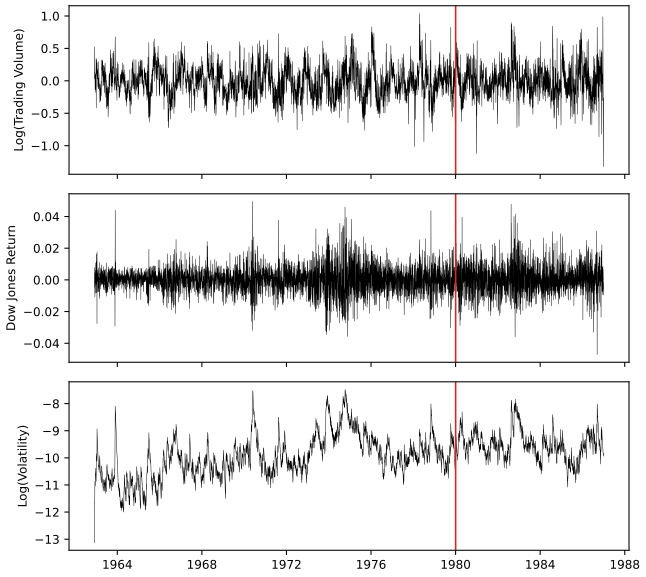
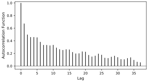
fig_10_14. Reproduces James et al. (2021), Figure 10.14. Download: PDF · SVGpp. 427–428 Unlike the other data sets of the book, the observations are not independent: nearby days are similar. The autocorrelation at lag \(\ell\) is the correlation of the pairs \((v_t,v_{t-\ell})\); Figure 10.15 shows it for log volume, above 0.2 even 20 days apart (0.226 at lag 20).
acf(). Code: fig_10_15, acf. Reproduces James et al. (2021), Figure 10.15. Download: PDF · SVGpp. 428–429 RNN forecaster. There is a single long series rather than 25,000 documents, and the response is itself a predictor. The trick is to cut the series into many short pieces. For each day \(t\) the input is the sequence of the previous \(L\) days' measurements and the target is today's volume:
\[ X_1=\begin{pmatrix}v_{t-L}\\r_{t-L}\\z_{t-L}\end{pmatrix},\ X_2=\begin{pmatrix}v_{t-L+1}\\r_{t-L+1}\\z_{t-L+1}\end{pmatrix},\ \cdots,\ X_L=\begin{pmatrix}v_{t-1}\\r_{t-1}\\z_{t-1}\end{pmatrix},\quad Y=v_t. \tag{10.20} \]With \(L=5\) this gives one \((X,Y)\) pair for each \(t=6,\dots,6051\): 6,046 pairs, 4,276 of them in the training period and 1,770 in the test period. Forecasting the test days uses test-period data in the inputs, but only the past, so this is not cheating.
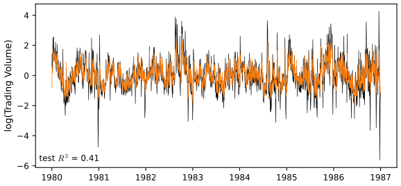
fig_10_16, rnn_forecast. Reproduces James et al. (2021), Figure 10.16. Download: PDF · SVGDefinition 10.9 (autoregression) p. 430, (10.21)–(10.22)
The order-\(L\) autoregressive model AR(\(L\)) is the least-squares regression of
\[ \by=\begin{bmatrix}v_{L+1}\\v_{L+2}\\v_{L+3}\\\vdots\\v_T\end{bmatrix}\quad\text{on}\quad \bM=\begin{bmatrix}1&v_L&v_{L-1}&\cdots&v_1\\1&v_{L+1}&v_L&\cdots&v_2\\1&v_{L+2}&v_{L+1}&\cdots&v_3\\\vdots&\vdots&\vdots&\ddots&\vdots\\1&v_{T-1}&v_{T-2}&\cdots&v_{T-L}\end{bmatrix}, \tag{10.21} \]both with \(T-L\) rows, that is, the model
\[ \hat v_t=\hat\beta_0+\hat\beta_1v_{t-1}+\hat\beta_2v_{t-2}+\dots+\hat\beta_Lv_{t-L}. \tag{10.22} \]With the lags of \(r_t\) and \(z_t\) added, \(\bM\) has \(3L+1\) columns: the RNN's input sequence, flattened into one long vector.
pp. 430–431 On the NYSE data, AR(5) on all three series has test \(R^2=0.4132\), the RNN about 0.42 (205 parameters against the AR model's 16), and a nonlinear AR model (a one-hidden-layer network on the 15 lagged inputs) 0.42. Adding the day of the week of the target day (volume is higher on Mondays and Fridays) as five dummy variables lifts AR to 0.4599 and the nonlinear AR model to about 0.47. The lab reproduces all of these; the deterministic AR numbers agree with the book to all printed digits in both languages.
Filling the gap 10.8: the test \(R^2\), and why the two editions print 0.4132 and 0.4129 for the same model p. 456 (R) and p. 461 (Python)
Derivation
Both labs fit the same AR(5) by least squares and compute the test \(R^2=1-\mathrm{MSE}_{\text{test}}/V\), as in (3.17), but with different \(V\). The R lab divides by var(), the sample variance with denominator \(n-1\) (\(n=1770\) test days); the Python lab uses scikit-learn's score(), which divides by \(\frac1n\sum(y_i-\bar y)^2\). Since the second \(V\) is \((n-1)/n\) times the first,
so \(R^2_{\text{Python}}=0.4129\): the printed numbers differ, the fits do not. (The same holds for the model with the day of the week: 0.4599 and 0.4596, printed as 0.4595 in the Python edition.) Two smaller points: the R lab standardises with \(n-1\) and scikit-learn's StandardScaler with \(n\), which rescales every column by the same factor and leaves least-squares predictions on the standardised scale unchanged; and a linear AR model fitted through the "flattened" RNN input of Exercise 10 is the same regression with its columns reordered, so its \(R^2\) is identical.
See also: the lagged-returns logistic regressions on the Smarket data in Chapter 4, Section 4.7.
10.5.3 Summary of RNNs
p. 431 Variants include one-dimensional convolutional networks that slide a filter along the sequence, several stacked recurrent layers, bidirectional RNNs that read the sequence both ways, and Seq2Seq models for translation, whose input and output are both sequences. Good software hides most of the complexity of fitting them.
10.6 When to Use Deep Learning
pp. 432–433 Should we use deep learning for everything? On the Hitters data of Chapter 6 (263 players with a known 1987 salary, 19 predictors), split into 176 training and 87 test players, three methods give similar test errors:
| Model | # parameters | Mean abs. error, book | here | Test \(R^2\), book | here |
|---|---|---|---|---|---|
| Linear regression | 20 | 254.7 | 254.7 | 0.56 | 0.566 |
| Lasso | 12 (here 13) | 252.3 | 252.3 | 0.51 | 0.522 |
| Neural network | 1409 | 257.4 | 253.8 | 0.54 | 0.564 |
Table 10.2, recomputed on the test players of the R lab (set.seed(13)). The lasso's \(\lambda\) minimises the ten-fold cross-validated mean absolute error (fixed folds here, random folds in the book: with the book's own call, current glmnet gives 252.30 with 13 nonzero coefficients). The network has 64 ReLU units, 10% dropout, and is fitted by RMSprop with minibatches of 32 for 1000 epochs, the settings of the book's footnote 21; its numbers vary from run to run by a few units.
pp. 432–433 The network needed fiddling to match the linear models, which are easier to fit, to present and to understand. By Occam's razor, among methods that perform about equally, pick the simplest. A four-variable model (Hits, Walks, CRuns, PutOuts) found by further exploration with the lasso and refitted by least squares on the training players (a relaxed lasso) did better still; the book reports a test MAE of 224.8, but the same model fitted on these training players gives 234.7 (see Notes on the book). Its coefficients should not be reported with \(p\)-values from the training data, because the variables were selected there; Table 10.3 refits it on the test players, which were not used in the selection:
| Coefficient | Std. error | \(t\)-statistic | \(p\)-value | |
|---|---|---|---|---|
| Intercept | −226.67 | 86.26 | −2.63 | 0.0103 |
| Hits | 3.06 | 1.02 | 3.00 | 0.0036 |
| Walks | 0.181 | 2.04 | 0.09 | 0.9295 |
| CRuns | 0.859 | 0.12 | 7.09 | < 0.0001 |
| PutOuts | 0.465 | 0.13 | 3.60 | 0.0005 |
Table 10.3, recomputed: least squares of Salary on the four variables, fitted on the 87 test players. Every entry agrees with the book's table (its 0.9294 for Walks is 0.92948 truncated, like the \(R^2\) of Table 10.2), which confirms that the test set here is the book's.
p. 433 Deep learning is attractive when the training set is very large and interpretability is not a priority.
See also: the lasso and cross-validation on the same data in Chapter 6, Section 6.5.2.
10.7 Fitting a Neural Network
p. 434 For the single-layer network the parameters are \(\beta=(\beta_0,\dots,\beta_K)\) and \(w_k=(w_{k0},\dots,w_{kp})\), and fitting is the nonlinear least-squares problem
\[ \operatorname*{minimize}_{\{w_k\}_1^K,\,\beta}\ \frac12\sum_{i=1}^n\big(y_i-f(x_i)\big)^2, \tag{10.23} \] \[ f(x_i)=\beta_0+\sum_{k=1}^K\beta_kg\Big(w_{k0}+\sum_{j=1}^pw_{kj}x_{ij}\Big). \tag{10.24} \]The problem is not convex: there are many local minima, partly because of the symmetry of the hidden units (permuting them, or for odd activations flipping signs, gives the same \(f\)). Two strategies keep the fit under control: slow learning by gradient descent, stopped when overfitting begins, and regularisation by penalties. With all parameters in one vector \(\bth\), the objective is
\[ R(\bth)=\frac12\sum_{i=1}^n\big(y_i-f_\bth(x_i)\big)^2. \tag{10.25} \]Algorithm 10.1 (gradient descent) pp. 434–436, (10.26)–(10.27), Figure 10.17
- Start with a guess \(\bth^0\) (typically random) and set \(t=0\).
- Until the objective (10.25) stops decreasing: compute the gradient at the current value, \[ \nabla R(\bth^t)=\frac{\partial R(\bth)}{\partial\bth}\Big|_{\bth=\bth^t}, \tag{10.26} \] the direction in which \(R\) increases fastest, and take a small step against it, \[ \bth^{t+1}\leftarrow\bth^t-\rho\nabla R(\bth^t), \tag{10.27} \] with learning rate \(\rho\); set \(t\leftarrow t+1\).
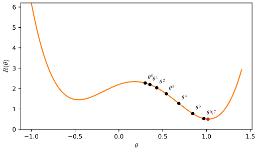
fig_10_17. Reproduces James et al. (2021), Figure 10.17. Download: PDF · SVG10.7.1 Backpropagation
pp. 435–436 Because \(R(\bth)=\sum_iR_i(\bth)\) is a sum, so is its gradient; consider one term,
\[ R_i(\bth)=\frac12\Big(y_i-\beta_0-\sum_{k=1}^K\beta_kg\Big(w_{k0}+\sum_{j=1}^pw_{kj}x_{ij}\Big)\Big)^2, \tag{10.28} \]and write \(z_{ik}=w_{k0}+\sum_jw_{kj}x_{ij}\). The chain rule gives
\[ \frac{\partial R_i(\bth)}{\partial\beta_k}=\frac{\partial R_i(\bth)}{\partial f_\bth(x_i)}\cdot\frac{\partial f_\bth(x_i)}{\partial\beta_k}=-\big(y_i-f_\bth(x_i)\big)\cdot g(z_{ik}), \tag{10.29} \] \[ \frac{\partial R_i(\bth)}{\partial w_{kj}}=\frac{\partial R_i(\bth)}{\partial f_\bth(x_i)}\cdot\frac{\partial f_\bth(x_i)}{\partial g(z_{ik})}\cdot\frac{\partial g(z_{ik})}{\partial z_{ik}}\cdot\frac{\partial z_{ik}}{\partial w_{kj}}=-\big(y_i-f_\bth(x_i)\big)\cdot\beta_k\cdot g'(z_{ik})\cdot x_{ij}. \tag{10.30} \]Both contain the residual \(y_i-f_\bth(x_i)\): differentiation hands a share of the residual to each parameter, first to each hidden unit in proportion to \(g(z_{ik})\), then through unit \(k\) to input \(j\). This is backpropagation.
Filling the gap 10.9: (10.29)–(10.30) step by step, and backpropagation through any number of layers p. 436, "it takes careful bookkeeping"
Derivation
The single layer. \(R_i=\frac12(y_i-f)^2\) with \(f=\beta_0+\sum_k\beta_kg(z_{ik})\), so \(\partial R_i/\partial f=-(y_i-f)\). Next, \(f\) depends on \(\beta_k\) only through the term \(\beta_kg(z_{ik})\), so \(\partial f/\partial\beta_k=g(z_{ik})\) (and \(\partial f/\partial\beta_0=1\)); multiplying gives (10.29). For \(w_{kj}\), the parameter sits inside \(z_{ik}\) only: \(\partial z_{ik}/\partial w_{kj}=x_{ij}\) (and \(\partial z_{ik}/\partial w_{k0}=1\)), \(\partial g(z_{ik})/\partial z_{ik}=g'(z_{ik})\), and \(\partial f/\partial g(z_{ik})=\beta_k\). Multiplying the four factors gives (10.30). For the ReLU, \(g'(z)=1\) if \(z>0\) and 0 if \(z\lt0\) (at \(z=0\) software uses 0): only active units pass the residual back. For the sigmoid, \(g'(z)=g(z)(1-g(z))\).
Computing it efficiently. Define the "error" of the output, \(\delta_i=-(y_i-f(x_i))\), and of hidden unit \(k\), \(s_{ik}=\delta_i\beta_kg'(z_{ik})\). Then \(\partial R_i/\partial\beta_k=\delta_iA_{ik}\) and \(\partial R_i/\partial w_{kj}=s_{ik}x_{ij}\): every gradient is (error at the receiving end) × (signal at the sending end). A forward pass computes the \(z_{ik}\) and \(A_{ik}\); a backward pass computes \(\delta_i\) and then the \(s_{ik}\) from it.
Many layers. For a network with layers \(A^{(0)}=x\), \(z^{(l)}=W^{(l)}A^{(l-1)}+b^{(l)}\), \(A^{(l)}=g(z^{(l)})\) (output layer linear), let \(s^{(l)}=\partial R_i/\partial z^{(l)}\). At the output, \(s^{(L)}=f-y\) for squared error and \(s^{(L)}=p-y\) (probabilities minus indicators) for softmax with cross-entropy (Filling the gap 10.3). The chain rule through \(z^{(l+1)}=W^{(l+1)}g(z^{(l)})+b^{(l+1)}\) gives the backward recursion and the gradients
\[ s^{(l)}=\big(W^{(l+1)\T}s^{(l+1)}\big)\odot g'\big(z^{(l)}\big),\qquad \frac{\partial R_i}{\partial W^{(l)}}=s^{(l)}A^{(l-1)\T},\qquad \frac{\partial R_i}{\partial b^{(l)}}=s^{(l)}, \]with \(\odot\) the elementwise product. For \(L=1\) hidden layer this is (10.29)–(10.30). One backward pass costs about as much as two forward passes, whatever the number of parameters, which is what makes networks with millions of weights trainable. The R lab's mlp_backward is exactly this recursion, for a minibatch at once (the rows of the matrices are the observations, so the sums over \(i\) become matrix products): crossprod(A, D) is \(\sum_iA^{(l-1)}_is^{(l)\T}_i\), and D %*% t(W) * (A > 0) is the recursion with the ReLU's \(g'\).
Confirmed numerically: on a random network (10.29)–(10.30) agree with PyTorch's automatic differentiation to \(10^{-12}\) and with central finite differences to \(10^{-6}\).
Deeper: Statistical Learning: Theory and Methods, Section 11.4 and Result 11.5 (back-propagation for squared error). See also: the backpropagation formulae, its cost and reverse-mode automatic differentiation in Foundations of Deep Learning, with its step-by-step demonstration.
10.7.2 Regularization and Stochastic Gradient Descent
pp. 436–437 Gradient descent takes many steps, and each step sums the gradients of all \(n\) observations. Stochastic gradient descent (SGD) instead uses a small random minibatch of observations for each step; it is the standard way to fit deep networks. An epoch is the number of steps needed to process \(n\) observations once: with 48,000 MNIST training images and minibatches of 128, \(48{,}000/128=375\) steps.
Filling the gap 10.10: why a small step goes downhill, and why a minibatch gradient points the right way on average pp. 435–437
Derivation
Downhill. By Taylor's theorem, for a step \(\bth^{t+1}=\bth^t-\rho\nabla R(\bth^t)\),
\[ R(\bth^{t+1})=R(\bth^t)-\rho\,\|\nabla R(\bth^t)\|^2+O(\rho^2), \]so if the gradient is not zero the objective decreases for every small enough \(\rho\). More precisely, if the gradient is \(L\)-Lipschitz (the curvature is at most \(L\)), then
\[ R(\bth^{t+1})\le R(\bth^t)-\rho\Big(1-\frac{L\rho}2\Big)\|\nabla R(\bth^t)\|^2, \]a decrease whenever \(\rho\lt2/L\). Too large a step overshoots (try a large rate in the Hitters demonstration). A zero gradient means a stationary point: a minimum, but possibly only a local one, or a saddle (Figure 10.17).
Unbiased minibatches. Let \(B\) be a minibatch of \(m\) observations drawn at random without replacement from the \(n\). Each observation is in \(B\) with probability \(m/n\), so
\[ \E\Big[\frac nm\sum_{i\in B}\nabla R_i(\bth)\Big]=\frac nm\sum_{i=1}^n\frac mn\nabla R_i(\bth)=\nabla R(\bth): \]the scaled minibatch gradient is an unbiased estimate of the full gradient, at \(1/(n/m)\) of the cost. Its variance shrinks like \(1/m\); the noise it adds is not all bad (it helps to leave poor local minima, and it acts as a mild regulariser). Software averages over the minibatch instead of scaling by \(n/m\), which only rescales \(\rho\).
Epochs. If \(m\) does not divide \(n\), the last step of an epoch uses the remainder: the Hitters training set of 176 players in minibatches of 32 takes 6 steps, five of 32 and one of 16 (the book's "5.5 steps" counts fractions), and the Python edition's 48,000 MNIST images in minibatches of 256 take 188 (187.5 rounded up).
See also: a small enough step always decreases the error, mean and variance of a minibatch gradient and RMSProp and Adam in Foundations of Deep Learning, with its optimiser paths demonstration.
p. 437 The MNIST network has about four times as many weights as training images, so regularisation is essential. The first row of Table 10.1 adds a ridge penalty to the cross-entropy,
\[ R(\bth;\lambda)=-\sum_{i=1}^n\sum_{m=0}^9y_{im}\log\big(f_m(x_i)\big)+\lambda\sum_j\theta_j^2, \tag{10.31} \]with \(\lambda\) small and preset, or chosen on a validation set; different \(\lambda\) can be used for different layers (here \(\bW_1\) and \(\bW_2\) were penalised and \(\bB\) was not). The penalty adds \(2\lambda\theta_j\) to each gradient, so every step first shrinks the weights by the factor \(1-2\rho\lambda\) and then moves against the gradient of the loss: hence the name weight decay. SGD itself acts as an approximately quadratic regulariser, and stopping it early is another form of regularisation: Figure 10.18 shows the validation objective rising after about 10 to 15 epochs while the training objective keeps falling.
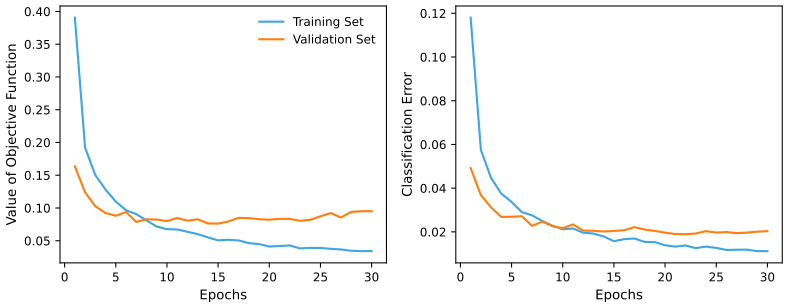
fig_10_18, mnist_results. Reproduces James et al. (2021), Figure 10.18. Download: PDF · SVGDeeper: Statistical Learning: Theory and Methods, Section 11.5.2 (overfitting, early stopping and weight decay) and Filling the gap 11.6 (in what sense weight decay is ridge regression). See also: early stopping is weight decay, up to a factor of 2 (Foundations of Deep Learning, Result 9.7) and its early stopping demonstration.
10.7.3 Dropout Learning
Definition 10.10 (dropout) p. 438, Figure 10.19
Each time a training observation is processed, each unit of a layer is removed independently with probability \(\phi\): its activation is set to zero, and the surviving activations are multiplied by \(1/(1-\phi)\) to compensate. At prediction time nothing is dropped. The idea, inspired by random forests (Section 8.2), is that units cannot rely on particular other units being present, so they do not become over-specialised.
Filling the gap 10.11: why the factor \(1/(1-\phi)\), and dropout as a ridge penalty p. 438, "similar in some respects to ridge regularization"
Derivation
Unbiasedness. Write the dropped activation as \(\tilde A=\frac{\delta}{1-\phi}A\) with \(\delta\sim\text{Bernoulli}(1-\phi)\). Then \(\E\tilde A=\frac{1-\phi}{1-\phi}A=A\): on average the next layer receives what it would receive without dropout, so the network can be used at prediction time with all units and no rescaling.
Dropout in linear regression is ridge. Apply dropout to the inputs of a linear model, with independent \(\delta_{ij}\sim\text{Bernoulli}(1-\phi)\) for every observation and input. The expected training loss is
\[ \E\sum_i\Big(y_i-\sum_j\frac{\delta_{ij}}{1-\phi}x_{ij}\beta_j\Big)^2=\sum_i\Big(y_i-\sum_jx_{ij}\beta_j\Big)^2+\sum_i\sum_j\Var\Big(\frac{\delta_{ij}}{1-\phi}\Big)x_{ij}^2\beta_j^2, \]because the mean of the prediction is \(x_i^\T\beta\) and its variance is the sum of the independent terms' variances (\(\E(Y-U)^2=(Y-\E U)^2+\Var U\)). With \(\Var(\delta/(1-\phi))=\phi(1-\phi)/(1-\phi)^2=\phi/(1-\phi)\),
\[ \E[\text{dropout loss}]=\sum_i\big(y_i-x_i^\T\beta\big)^2+\frac{\phi}{1-\phi}\sum_j\Big(\sum_ix_{ij}^2\Big)\beta_j^2. \]This is ridge regression with a separate penalty for each coefficient, proportional to the size of its input: for standardised inputs (\(\sum_ix_{ij}^2=n\)) exactly ridge with \(\lambda=n\phi/(1-\phi)\). In a network the correspondence is only approximate, but the message is the same: dropout shrinks.
Confirmed numerically: the exact expectation over all dropout patterns of a small problem equals the formula to \(10^{-12}\).
See also: dropout on a linear model is a data-dependent ridge penalty and dropout as model averaging (Foundations of Deep Learning), with its dropout and ensembles demonstration.
10.7.4 Network Tuning
pp. 438–439 Even the simple network of Figure 10.4 involves many choices: the number of hidden layers and of units per layer (modern practice: many units, with overfitting controlled by regularisation); the regularisation parameters (dropout rates, ridge and lasso \(\lambda\), possibly different in each layer); and the details of SGD (minibatch size, number of epochs, data augmentation). They matter: careful tuning of a similar network gets below 1% error on MNIST, but the tinkering is tedious, and tuning on the test set overfits it.
Deeper: Statistical Learning: Theory and Methods, Section 11.5 (starting values, scaling of the inputs, number of hidden units and layers, multiple minima).
10.8 Interpolation and Double Descent
pp. 439–440 The bias-variance trade-off (Section 2.2.2) says that test error is U-shaped in flexibility, and that interpolating the training data (zero training error) usually gives a high test error. In some settings, though, a method that interpolates does well, better than a slightly less flexible one that does not: double descent. The example has \(n=20\) observations from \(Y=\sin(X)+\epsilon\), \(X\sim U[-5,5]\), \(\epsilon\sim N(0,0.3^2)\), fitted by natural splines (Section 7.4) with \(d\) degrees of freedom, that is, least squares on \(d\) basis functions with knots at \(d\) quantiles of the training \(x\)'s. At \(d=20=n\) the spline interpolates. Beyond it the least-squares problem has infinitely many solutions with zero training error, and the one with the smallest \(\sum_j\hat\beta_j^2\), the minimum-norm solution, is chosen.
Definition 10.11 (minimum-norm least squares) p. 440
Let \(\bB\) be the \(n\times d\) matrix of the basis functions at the training points. Among all minimisers of \(\|\by-\bB\beta\|^2\), the minimum-norm solution is the one with the smallest \(\|\beta\|^2=\sum_j\beta_j^2\). If \(\bB\) has full column rank (\(d\le n\)) it is the ordinary least-squares solution; if \(\bB\) has full row rank (\(d\ge n\)) it interpolates the data and equals \(\hat\beta=\bB^\T(\bB\bB^\T)^{-1}\by\).
Filling the gap 10.12: the minimum-norm solution: formula, limit of ridge, and the end point of gradient descent pp. 440–442
Derivation
Formula. Suppose \(d\ge n\) and the rows of \(\bB\) are linearly independent, so \(\bB\bB^\T\) (\(n\times n\)) is invertible and interpolation \(\bB\beta=\by\) is possible. Every solution can be written \(\beta=\beta^*+v\) with \(\beta^*=\bB^\T(\bB\bB^\T)^{-1}\by\) (indeed \(\bB\beta^*=\by\)) and \(\bB v=0\). Since \(\beta^*\) is a combination of the rows of \(\bB\) and \(v\) is orthogonal to every row, \(\beta^{*\T}v=0\), and by Pythagoras \(\|\beta\|^2=\|\beta^*\|^2+\|v\|^2\ge\|\beta^*\|^2\), with equality only for \(v=0\). In general (any rank) the minimum-norm least-squares solution is \(\bB^+\by\) with the pseudo-inverse \(\bB^+\), which the code computes from an eigendecomposition of \(\bB^\T\bB\) or \(\bB\bB^\T\).
The limit of ridge. The ridge solution can be written \(\hat\beta_\lambda=(\bB^\T\bB+\lambda\bI)^{-1}\bB^\T\by=\bB^\T(\bB\bB^\T+\lambda\bI)^{-1}\by\) (multiply out \(\bB^\T(\bB\bB^\T+\lambda\bI)=(\bB^\T\bB+\lambda\bI)\bB^\T\)). As \(\lambda\downarrow0\) the right-hand form tends to \(\bB^\T(\bB\bB^\T)^{-1}\by\): the minimum-norm interpolant is ridge regression with a vanishing penalty, the least-regularised fit that still prefers small coefficients.
The implicit bias of gradient descent. Run gradient descent on \(\frac12\|\by-\bB\beta\|^2\) from \(\beta^0=0\). Each step adds \(\rho\bB^\T(\by-\bB\beta^t)\), a combination of the rows of \(\bB\), so every iterate stays in the row space of \(\bB\). If it converges (\(\rho\) small enough), the limit interpolates and lies in the row space, and the only such vector is \(\beta^*\) (the decomposition above with \(v=0\)). So gradient descent started at zero finds the minimum-norm solution without being told to: this is one sense in which "the techniques used to fit neural networks naturally lend themselves to selecting a smooth interpolating model" (p. 441). For networks the picture is only heuristic, since the model is not linear in its parameters.
Why \(\hat f_{20}\) is wild and \(\hat f_{42}\) is not. At \(d=n\) there is exactly one interpolant, and if \(\bB\) is nearly singular its coefficients are huge (norm 26.7 in our example, against 3.2 at \(d=8\)). With more basis functions there are many interpolants and the smallest one can be much smaller (norm 6.0 at \(d=42\)): small coefficients mean a fit that does not swing far between the data points. In variance terms, the minimum-norm fit with \(d=42\) has a lower variance than the one with \(d=20\), so the horizontal axis of Figure 10.20 is a poor measure of flexibility, and there is no contradiction with the bias-variance trade-off. The size of the coefficients against \(d\) is the bottom panel of the demonstration.
The signal-to-noise ratio. For \(X\sim U[-5,5]\), \(\E\sin X=0\) and
\[ \E\sin^2X=\frac1{10}\int_{-5}^5\frac{1-\cos2x}2\,dx=\frac12-\frac{\sin10}{20}=0.527, \]so \(\Var(f(X))/\sigma^2=0.527/0.09=5.86\), the book's 5.9.
Confirmed numerically: on a random 5 × 12 problem the formula, the pseudo-inverse, ridge with \(\lambda=10^{-10}\) and 20,000 steps of gradient descent from zero give the same \(\beta\).
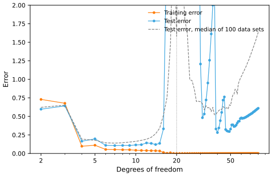
fig_10_20, ns_basis_full, min_norm_fit. Reproduces James et al. (2021), Figure 10.20. Download: PDF · SVG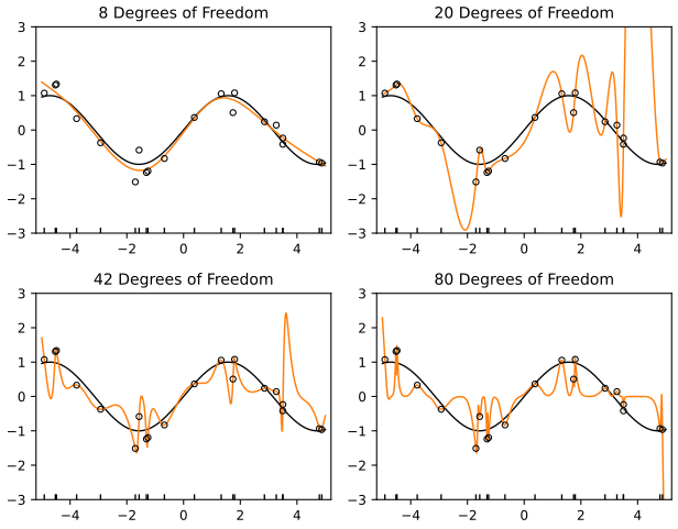
fig_10_21. Reproduces James et al. (2021), Figure 10.21. Download: PDF · SVGpp. 442–443 The book draws four lessons. (1) Double descent does not contradict the bias-variance trade-off; the number of basis functions is the wrong measure of flexibility for interpolating fits. (2) Most methods of the book do not show double descent, because regularised fits do not interpolate, and that is no drawback: here a ridge fit with a well-chosen \(\lambda\) beats every interpolating fit (in our example the curve of test error never exceeds 0.65 with \(\lambda=0.1\), against a best of 0.28 for the minimum-norm interpolants; the best fits of all are the small least-squares ones, about 0.11). (3) Maximal margin classifiers and SVMs also find smooth minimum-norm solutions with zero training error (Chapter 9). (4) Double descent is used to explain why huge networks trained to zero training error can work, but whether interpolation is advisable depends on the signal-to-noise ratio, and ridge penalties or early stopping avoid it while still doing very well.
Deeper: Statistical Learning: Theory and Methods, Section 18.3.5 (computing with \(\bB\bB^\T\) when \(p\gg N\), the same algebra as the minimum-norm solution) and Section 7.3 (the bias-variance decomposition). See also: the implicit bias of gradient descent, exact double descent for least squares with Gaussian inputs and double descent in training time in Foundations of Deep Learning; the bias-variance trade-off in Chapter 2, Section 2.2.2.
10.9 Lab: Deep Learning
p. 443 The lab fits the examples of the chapter. The two editions use different software: the R lab of James et al. 2021 uses the keras package, which drives TensorFlow through a Python installation; the Python lab of James et al. 2023 uses PyTorch with pytorch_lightning, torchvision and the authors' helper package. Here the R version writes the networks out in base R, and the Python version uses plain PyTorch with a short training loop; both use the same architectures, optimiser (RMSprop) and settings, taken from the R lab. The complete files are code/ch10_lab.R (about three minutes) and code/ch10_lab.py (about two and a half minutes, on one CPU thread); the excerpts below are taken from them verbatim, except that lines which only record a number in cache/ are left out.
Where the two languages differ, and why
- No keras in R. The keras and torch R packages need a separate deep-learning back end. The R lab here instead defines a dense network as a list of weight matrices, with a forward pass, backpropagation (Filling the gap 10.9), dropout and RMSprop in about sixty lines of base R, and a recurrent network with backpropagation through time in thirty more. On these problems it is fast enough (R's matrix products use the system's BLAS): the MNIST network trains in under two minutes.
- Same numbers. Everything deterministic agrees: the Hitters test set (R's
set.seed(13)split, used in both languages), least squares (test MAE 254.6687, the book's number), the lasso with fixed folds (\(\lambda=5.6924\), MAE 252.3386 in both once glmnet is run to full convergence), the AR models (0.4132 and 0.4599, the R lab's numbers), and Exercises 6, 7 (logistic regression), 9 and 10. - Similar numbers. The networks start from random weights and use random minibatches and dropout masks, drawn by different generators in R and PyTorch, so they agree only roughly: MNIST test accuracy 0.9810 and 0.9809, multinomial logistic regression 0.9268 and 0.9250, NYSE RNN \(R^2\) 0.4139 and 0.4164, nonlinear AR 0.4683 and 0.4649 (R, then Python). Neither language reproduces the book's runs exactly; the book itself warns that keras results vary from run to run.
- The book's two labs differ too. The Python edition splits Hitters with
train_test_split(random_state=1), so its least-squares MAE is 259.7 rather than 254.7, and builds 19 input columns rather than R's 20 (Filling the gap 10.2); it trains the MNIST network with minibatches of 256 and learning rate 0.01 (default of its helper) rather than 128 and 0.001; and it prints \(R^2\) with an \(n\) rather than \(n-1\) denominator (Filling the gap 10.8). Its RNN has 217 parameters against keras's 205 (two bias vectors, Filling the gap 10.7), and the R lab's RNN applies dropout to the inputs and the recurrent state, the Python lab's to the last hidden state (as here, in both languages). - Python only. The convolutional networks of Section 10.9.3: the CIFAR100 network is built and its 964,516 parameters counted, but not trained (the data are a 160 MB download and training takes over ten minutes); a small CNN is trained on MNIST instead. Writing convolutions and their gradients in base R is possible but would be slow and is not needed to follow the ideas.
- Not run in either language. The pretrained ResNet50 (10.9.4) needs
torchvisionand its 100 MB of weights; the IMDb models (10.9.5 and the LSTM of 10.9.6) need the IMDb corpus. These sections are described in words.
10.9.1 A Single Layer Network on the Hitters Data
The split and least squares. The test set is a random third of the 263 players. The Python lab uses the same players as R, listed in TESTID; least squares then gives the same test MAE, 254.6687, in both languages.
R
Gitters <- na.omit(Hitters)
n <- nrow(Gitters)
set.seed(13)
ntest <- trunc(n / 3)
testid <- sample(1:n, ntest)
cat("test players:", head(testid, 10), "...\n")

lfit <- lm(Salary ~ ., data = Gitters[-testid, ])
lpred <- predict(lfit, Gitters[testid, ])
mae_lm <- with(Gitters[testid, ], mean(abs(lpred - Salary)))
cat("least squares: test MAE", mae_lm, "\n")
Python
Hitters = common.isl_data("Hitters").dropna().reset_index(drop=True)
n = len(Hitters)
test = np.zeros(n, bool)
test[TESTID - 1] = True

Xlm = pd.get_dummies(Hitters.drop(columns=["Salary"]), drop_first=True, dtype=float)
Xlm.insert(0, "intercept", 1.0)
Y = Hitters["Salary"].to_numpy()
beta = np.linalg.lstsq(Xlm[~test].to_numpy(), Y[~test], rcond=None)[0]
mae_lm = np.abs(Xlm[test].to_numpy() @ beta - Y[test]).mean()
print("least squares: test MAE %.4f" % mae_lm)
The lasso. The predictors are standardised over all 263 players (as in the book) and the lasso's \(\lambda\) minimises the ten-fold cross-validated mean absolute error. With the book's random folds R gives 252.30 (the book: 252.2994). Both languages then use fixed folds (training row \(i\) in fold \(i\bmod10\)) so that they can be compared; lasso_glmnet reproduces glmnet's standardisation, objective and \(\lambda\) sequence with scikit-learn's coordinate descent.
R
x <- scale(model.matrix(Salary ~ . - 1, data = Gitters))   # 20 columns: both League dummies
y <- Gitters$Salary
cvfit <- cv.glmnet(x[-testid, ], y[-testid], type.measure = "mae")   # random folds, as in the book
cpred <- predict(cvfit, x[testid, ], s = "lambda.min")
cat("lasso, random folds: test MAE", mean(abs(y[testid] - cpred)), "\n")
foldid <- (seq_len(n - ntest) - 1) %% 10 + 1                    # fixed folds: training row i in fold i mod 10
cvfit2 <- cv.glmnet(x[-testid, ], y[-testid], type.measure = "mae", foldid = foldid,
                    control = list(thresh = 1e-12))            # converge fully, to compare with Python
cpred2 <- predict(cvfit2, x[testid, ], s = "lambda.min")
cat("lasso, fixed folds: lambda.min", cvfit2$lambda.min, " test MAE", mean(abs(y[testid] - cpred2)),
    " nonzero coefficients", sum(coef(cvfit2, s = "lambda.min")[-1] != 0), "\n")
Python
M = hitters_matrix(Hitters)
X = ((M - M.mean()) / M.std()).to_numpy()            # R's scale(): 1/(n-1) standard deviations
print("model matrix:", X.shape, list(M.columns[13:17]))
Xtr, Ytr, Xte, Yte = X[~test], Y[~test], X[test], Y[test]
lambdas, _, _ = lasso_glmnet(Xtr, Ytr)
fold = np.arange(len(Ytr)) % 10                      # training row i in fold i mod 10, as foldid in R
abs_err = np.zeros((len(Ytr), len(lambdas)))
for k in range(10):
    _, b0, B = lasso_glmnet(Xtr[fold != k], Ytr[fold != k], lambdas)
    abs_err[fold == k] = np.abs(Ytr[fold == k, None] - (b0 + Xtr[fold == k] @ B))
best = np.argmin(abs_err.mean(0))
_, b0, B = lasso_glmnet(Xtr, Ytr, lambdas)
mae_lasso = np.abs(Yte - (b0[best] + Xte @ B[:, best])).mean()
print("lasso, fixed folds: lambda.min %.4f  test MAE %.4f  nonzero coefficients %d"
      % (lambdas[best], mae_lasso, np.sum(B[:, best] != 0)))
The helper functions: hitters_matrix and lasso_glmnet (Python)
def lasso_glmnet(X, y, lambdas=None, nlambda=100):
    """The lasso path on glmnet's scale: columns standardised with their 1/n standard deviation,
    objective RSS/(2n) + lambda * sum|beta_j|, glmnet's default lambda sequence. Returns
    (lambdas, intercepts, coefficients on the original scale, one column per lambda)."""
    mx, sx = X.mean(0), X.std(0)
    Z, yc = (X - mx) / sx, y - y.mean()
    if lambdas is None:
        lmax = np.abs(Z.T @ yc).max() / len(y)
        ratio = 1e-4 if len(y) > X.shape[1] else 1e-2
        lambdas = lmax * np.exp(np.linspace(0, np.log(ratio), nlambda))
    _, coefs, _ = skl.lasso_path(Z, yc, alphas=lambdas, tol=1e-12, max_iter=200000)
    B = coefs / sx[:, None]
    return lambdas, y.mean() - mx @ B, B

def hitters_matrix(H):
    """R's model.matrix(Salary ~ . - 1): without an intercept the first factor (League) keeps both of its
    dummies, LeagueA and LeagueN; the later factors drop their first level (DivisionW, NewLeagueN)."""
    cols, first = {}, True
    for c in H.columns.drop("Salary"):
        if H[c].dtype == object:
            levels = sorted(H[c].unique())
            for lev in (levels if first else levels[1:]):
                cols[c + lev] = (H[c] == lev).to_numpy(float)
            first = False
        else:
            cols[c] = H[c].to_numpy(float)
    return pd.DataFrame(cols)
The network. One hidden layer of 50 ReLU units with 40% dropout, fitted by RMSprop (learning rate 0.001) on minibatches of 32 for 1500 epochs, tracking the training and test MAE after every epoch. The test set serves as validation data only to draw the curves, not to choose anything.
R
set.seed(1)
modnn <- mlp_init(c(ncol(x), 50, 1))                 # 20 inputs -> 50 ReLU units -> 1 output
cat("parameters:", n_params(modnn), "\n")            # 50 * 21 + 51 = 1101
xtr <- x[-testid, ]; ytr <- y[-testid]; xte <- x[testid, ]; yte <- y[testid]
hit <- fit_mlp(modnn, xtr, ytr, loss = "mse", epochs = 1500, batch_size = 32, lr = 0.001, dropout = 0.4,
               monitor = function(net) c(train_mae = mean(abs(predict_mlp(net, xtr) - ytr)),
                                         test_mae = mean(abs(predict_mlp(net, xte) - yte))))
npred <- predict_mlp(hit$net, xte)
cat("neural network: test MAE", mean(abs(yte - npred)), "\n")
Python
torch.manual_seed(1)
hit_model = nn.Sequential(nn.Linear(X.shape[1], 50), nn.ReLU(), nn.Dropout(0.4), nn.Linear(50, 1))
print("parameters:", n_params(hit_model))           # 50 * 21 + 51 = 1101
Xtr_t, Ytr_t, Xte_t, Yte_t = tensor(Xtr), tensor(Ytr), tensor(Xte), tensor(Yte)
hist = fit(hit_model, Xtr_t, Ytr_t, mse, epochs=1500, batch_size=32, lr=0.001,
           monitor=lambda m: {"train_mae": float((m(Xtr_t).flatten() - Ytr_t).abs().mean()),
                              "test_mae": float((m(Xte_t).flatten() - Yte_t).abs().mean())})
with torch.no_grad():
    mae_nn = float((hit_model(Xte_t).flatten() - Yte_t).abs().mean())
print("neural network: test MAE %.4f" % mae_nn)
The neural-network toolkit of the R lab: forward pass, backpropagation, RMSprop and the training loop
# A network is a list of layers, each with a weight matrix W (inputs x units) and a bias vector b.
# Hidden layers use ReLU; the output layer is linear (a prediction, or the logits Z_m of (10.12)).
relu <- function(z) pmax(z, 0)
init_layer <- function(fan_in, fan_out) {     # the default of torch's nn.Linear: U(-1/sqrt(fan_in), +)
  s <- 1 / sqrt(fan_in)
  list(W = matrix(runif(fan_in * fan_out, -s, s), fan_in, fan_out), b = runif(fan_out, -s, s))
}
mlp_init <- function(sizes) lapply(seq_len(length(sizes) - 1), function(l) init_layer(sizes[l], sizes[l + 1]))
n_params <- function(net) sum(sapply(net, function(layer) length(layer$W) + length(layer$b)))

mlp_forward <- function(net, X, dropout = 0, train = FALSE) {
  L <- length(net); A <- vector("list", L + 1); M <- vector("list", L); A[[1]] <- X
  dropout <- rep_len(dropout, L)
  for (l in 1:L) {
    Z <- A[[l]] %*% net[[l]]$W + rep(net[[l]]$b, each = nrow(A[[l]]))
    if (l < L) {
      Z <- relu(Z)
      if (train && dropout[l] > 0) {          # dropout (Section 10.7.3): zero a fraction phi, scale by 1/(1-phi)
        M[[l]] <- (runif(length(Z)) > dropout[l]) / (1 - dropout[l])
        Z <- Z * M[[l]]
      }
    }
    A[[l + 1]] <- Z
  }
  list(A = A, M = M)
}

# Backpropagation: dOut is the derivative of the loss with respect to the network's output.
# Layer by layer this is the chain rule of (10.29)-(10.30): the gradient of W is
# (inputs of the layer)' x (derivative at its output), and the derivative is passed back through W'
# and multiplied by g'(z), which for ReLU is 1 where the unit was active and 0 elsewhere.
mlp_backward <- function(net, fw, dOut) {
  L <- length(net); G <- vector("list", L); D <- dOut
  for (l in L:1) {
    G[[l]] <- list(W = crossprod(fw$A[[l]], D), b = colSums(D))
    if (l > 1) {
      D <- D %*% t(net[[l]]$W)
      if (!is.null(fw$M[[l - 1]])) D <- D * fw$M[[l - 1]]
      D <- D * (fw$A[[l]] > 0)
    }
  }
  G
}

softmax <- function(Z) { E <- exp(Z - apply(Z, 1, max)); E / rowSums(E) }

# RMSprop with torch's defaults (alpha = 0.99, eps = 1e-8): each weight's step is the gradient divided
# by a running root-mean-square of its past gradients.
rmsprop_step <- function(net, G, V, lr, alpha = 0.99, eps = 1e-8) {
  for (l in seq_along(net)) for (nm in c("W", "b")) {
    V[[l]][[nm]] <- alpha * V[[l]][[nm]] + (1 - alpha) * G[[l]][[nm]]^2
    net[[l]][[nm]] <- net[[l]][[nm]] - lr * G[[l]][[nm]] / (sqrt(V[[l]][[nm]]) + eps)
  }
  list(net = net, V = V)
}

# Minibatch training. loss = "mse" (quantitative y), "xent" (y a 0/1 matrix, softmax output) or
# "logit" (binary y, one logit output). monitor(net) is called after every epoch.
fit_mlp <- function(net, X, y, loss, epochs, batch_size, lr = 0.001, dropout = 0, monitor = NULL) {
  y <- as.matrix(y); n <- nrow(X)
  V <- lapply(net, function(layer) list(W = 0 * layer$W, b = 0 * layer$b))
  hist <- NULL
  for (ep in 1:epochs) {
    perm <- sample.int(n)
    for (s in seq(1, n, by = batch_size)) {
      idx <- perm[s:min(s + batch_size - 1, n)]
      fw <- mlp_forward(net, X[idx, , drop = FALSE], dropout, train = TRUE)
      out <- fw$A[[length(net) + 1]]
      dOut <- switch(loss,
        mse = 2 * (out - y[idx, , drop = FALSE]) / length(idx),
        xent = (softmax(out) - y[idx, , drop = FALSE]) / length(idx),
        logit = (1 / (1 + exp(-out)) - y[idx, , drop = FALSE]) / length(idx))
      st <- rmsprop_step(net, mlp_backward(net, fw, dOut), V, lr)
      net <- st$net; V <- st$V
    }
    if (!is.null(monitor)) hist <- rbind(hist, c(epoch = ep, monitor(net)))
  }
  list(net = net, history = as.data.frame(hist))
}
predict_mlp <- function(net, X) mlp_forward(net, X)$A[[length(net) + 1]]
The training loop of the Python lab: fit
def fit(model, X, y, loss_fn, epochs, batch_size, lr=0.001, monitor=None, seed=0):
    """Minibatch RMSprop (torch's defaults, as the R lab's rmsprop_step). monitor(model) is called
    after every epoch, in evaluation mode (dropout switched off); returns its values as a DataFrame."""
    gen = torch.Generator().manual_seed(seed)
    opt = torch.optim.RMSprop(model.parameters(), lr=lr)
    n, rows = len(y), []
    for epoch in range(1, epochs + 1):
        model.train()
        perm = torch.randperm(n, generator=gen)
        for s in range(0, n, batch_size):
            idx = perm[s:s + batch_size]
            opt.zero_grad()
            loss_fn(model(X[idx]), y[idx]).backward()
            opt.step()
        if monitor is not None:
            model.eval()
            with torch.no_grad():
                rows.append(dict(epoch=epoch, **monitor(model)))
    model.eval()
    return pd.DataFrame(rows)
test players: 259 74 205 132 221 248 55 23 5 140 ... least squares: test MAE 254.669 lasso, random folds: test MAE 252.298 lasso, fixed folds: lambda.min 5.69237 test MAE 252.339 nonzero coefficients 13 parameters: 1101 neural network: test MAE 252.115
least squares: test MAE 254.6687
model matrix: (263, 20) ['LeagueA', 'LeagueN', 'DivisionW', 'PutOuts']
lasso, fixed folds: lambda.min 5.6924  test MAE 252.3386  nonzero coefficients 13
parameters: 1101
neural network: test MAE 253.4896
The network's test MAE (252.1 in R, 253.5 in Python) is of the same size as least squares and the lasso, as in Table 10.2; the book's keras run gave 257.43. Both curves fall steeply over the first 250 epochs; after that the training error keeps creeping down while the test error flattens out near 250. (The training error is computed at the end of each epoch with dropout switched off.)
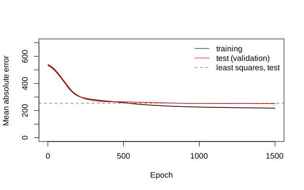
lab-r-hitters.svg.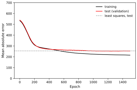
lab-py-hitters.svg.10.9.2 A Multilayer Network on the MNIST Digit Data
The data. In R the four MNIST files are read with readBin; in Python with common.mnist. The pixels are divided by 255, and in R the labels are one-hot encoded.
R
read_idx <- function(path) {
  con <- gzfile(path, "rb"); on.exit(close(con))
  magic <- readBin(con, "integer", 1, size = 4, endian = "big")
  dims <- readBin(con, "integer", magic %% 256, size = 4, endian = "big")
  v <- readBin(con, "integer", prod(dims), size = 1, signed = FALSE)
  if (length(dims) == 1) v else matrix(v, dims[1], prod(dims[-1]), byrow = TRUE)
}
mnist_file <- function(name) {
  dir <- file.path(Sys.getenv("ISL_CACHE", file.path(Sys.getenv("HOME"), ".cache", "prml-repro")), "mnist")
  path <- file.path(dir, name)
  if (!file.exists(path)) {
    dir.create(dir, showWarnings = FALSE, recursive = TRUE)
    download.file(paste0("https://ossci-datasets.s3.amazonaws.com/mnist/", name), path, mode = "wb")
  }
  path
}
x_train <- read_idx(mnist_file("train-images-idx3-ubyte.gz")) / 255   # 60000 x 784, rows are images
g_train <- read_idx(mnist_file("train-labels-idx1-ubyte.gz"))
x_test <- read_idx(mnist_file("t10k-images-idx3-ubyte.gz")) / 255
g_test <- read_idx(mnist_file("t10k-labels-idx1-ubyte.gz"))
cat("MNIST:", dim(x_train), "training,", dim(x_test), "test\n")
one_hot <- function(g, K = 10) { Y <- matrix(0, length(g), K); Y[cbind(seq_along(g), g + 1)] <- 1; Y }
y_train <- one_hot(g_train)
Python
x_train, g_train = common.mnist(train=True)          # 60000 x 784, pixel values scaled to [0, 1]
x_test, g_test = common.mnist(train=False)
print("MNIST:", x_train.shape, "training,", x_test.shape, "test")
fit_rows = np.arange(48000)                          # the last 20% are the validation set
val = np.arange(48000, 60000)
Xm, Gm = tensor(x_train), torch.tensor(g_train)
Xm_test, Gm_test = tensor(x_test), torch.tensor(g_test)
The network of Figure 10.4, with dropout 0.4 and 0.3 after the two hidden layers, 30 epochs, minibatches of 128, the last 12,000 training images as validation data (as keras's validation_split = 0.2), and accuracy tracked by epoch.
R
val <- 48001:60000                         # the last 20% of the training images, as validation_split = 0.2
accuracy <- function(pred, truth) mean(drop(pred) == drop(truth))
classes <- function(net, X) max.col(predict_mlp(net, X), ties.method = "first") - 1
set.seed(2)
modelnn <- mlp_init(c(784, 256, 128, 10))
cat("parameters:", n_params(modelnn), "\n")         # 200960 + 32896 + 1290 = 235146
t0 <- proc.time()[["elapsed"]]
mn <- fit_mlp(modelnn, x_train[-val, ], y_train[-val, ], loss = "xent", epochs = 30, batch_size = 128,
              lr = 0.001, dropout = c(0.4, 0.3),
              monitor = function(net) c(train_acc = accuracy(classes(net, x_train[1:12000, ]), g_train[1:12000]),
                                        valid_acc = accuracy(classes(net, x_train[val, ]), g_train[val])))
cat("fitting took", round(proc.time()[["elapsed"]] - t0), "seconds\n")
acc_nn <- accuracy(classes(mn$net, x_test), g_test)
cat("two hidden layers with dropout: test accuracy", acc_nn, "\n")
Python
def accuracy(model, X, g):
    with torch.no_grad():
        return float((model(X).argmax(1) == g).float().mean())

torch.manual_seed(2)
mnist_model = nn.Sequential(nn.Linear(784, 256), nn.ReLU(), nn.Dropout(0.4),
                            nn.Linear(256, 128), nn.ReLU(), nn.Dropout(0.3),
                            nn.Linear(128, 10))
print("parameters:", n_params(mnist_model))         # 200960 + 32896 + 1290 = 235146
t0 = time.time()
mhist = fit(mnist_model, Xm[fit_rows], Gm[fit_rows], nn.functional.cross_entropy, epochs=30, batch_size=128,
            lr=0.001, monitor=lambda m: {"train_acc": accuracy(m, Xm[:12000], Gm[:12000]),
                                         "valid_acc": accuracy(m, Xm[val], Gm[val])})
print("fitting took %.0f seconds" % (time.time() - t0))
acc_nn = accuracy(mnist_model, Xm_test, Gm_test)
print("two hidden layers with dropout: test accuracy %.4f" % acc_nn)
Multinomial logistic regression is the same network without hidden layers.
R
set.seed(3)
modellr <- mlp_init(c(784, 10))                     # no hidden layer: multinomial logistic regression
cat("parameters:", n_params(modellr), "\n")         # 785 * 10 = 7850
lr_fit <- fit_mlp(modellr, x_train[-val, ], y_train[-val, ], loss = "xent", epochs = 30, batch_size = 128, lr = 0.001)
acc_lr <- accuracy(classes(lr_fit$net, x_test), g_test)
cat("multinomial logistic regression: test accuracy", acc_lr, "\n")
Python
torch.manual_seed(3)
mlr_model = nn.Linear(784, 10)                       # no hidden layer: multinomial logistic regression
print("parameters:", n_params(mlr_model))           # 785 * 10 = 7850
fit(mlr_model, Xm[fit_rows], Gm[fit_rows], nn.functional.cross_entropy, epochs=30, batch_size=128, lr=0.001)
acc_lr = accuracy(mlr_model, Xm_test, Gm_test)
print("multinomial logistic regression: test accuracy %.4f" % acc_lr)
MNIST: 60000 784 training, 10000 784 test parameters: 235146 fitting took 109 seconds two hidden layers with dropout: test accuracy 0.981 parameters: 7850 multinomial logistic regression: test accuracy 0.9268
MNIST: (60000, 784) training, (10000, 784) test
parameters: 235146
fitting took 19 seconds
two hidden layers with dropout: test accuracy 0.9809
parameters: 7850
multinomial logistic regression: test accuracy 0.9250
Both languages reach 98.1% test accuracy with the network (the book's R lab: 0.9813; the Python edition, with its other settings: 0.9681) and about 92.5–92.7% with multinomial logistic regression (the book: 0.9286 and 0.9241).
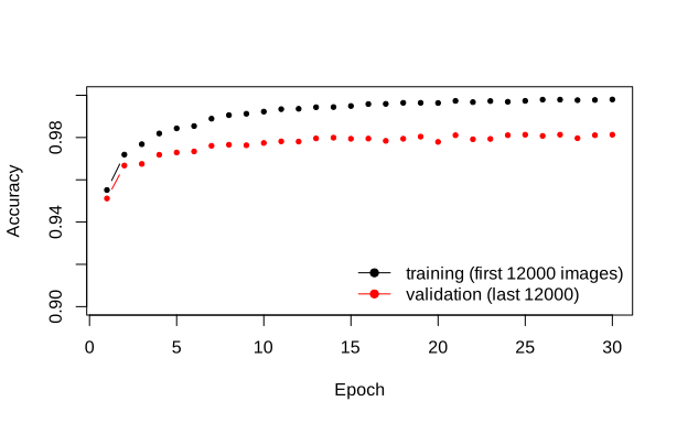
lab-r-mnist.svg.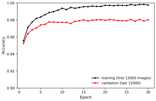
lab-py-mnist.svg.10.9.3 Convolutional Neural Networks
Python only
This section is not in the R lab: base R has no convolution layers, and writing their gradients by hand would add much code and run slowly. The ideas (convolution, the ReLU detector, pooling, the parameter counts) are in Section 10.3 and in the convolution demonstration.
The CIFAR100 network: four blocks of 3 × 3 convolution (padding "same"), ReLU and 2 × 2 max pooling, with 32, 64, 128 and 256 filters, then dropout, a dense layer of 512 units and the 100-class output. It is built and pushed through a dummy image to print each layer's output shape and parameters; the CIFAR100 data are not downloaded and the network is not trained (the book reports 10 minutes or more and a test accuracy of 46%, or 42% in the Python edition).
Python
class BuildingBlock(nn.Module):
    """3 x 3 convolution with 'same' padding, ReLU, then 2 x 2 max pooling."""
    def __init__(self, in_channels, out_channels):
        super().__init__()
        self.conv = nn.Conv2d(in_channels, out_channels, kernel_size=3, padding="same")
        self.pool = nn.MaxPool2d(2)

    def forward(self, x):
        return self.pool(torch.relu(self.conv(x)))

cifar_model = nn.Sequential(BuildingBlock(3, 32), BuildingBlock(32, 64), BuildingBlock(64, 128),
                            BuildingBlock(128, 256), nn.Flatten(), nn.Dropout(0.5),
                            nn.Linear(2 * 2 * 256, 512), nn.ReLU(), nn.Linear(512, 100))
shape = torch.zeros(1, 3, 32, 32)
for layer in cifar_model:
    shape = layer(shape)
    print("  %-14s output %-18s parameters %d" % (type(layer).__name__, tuple(shape.shape[1:]), n_params(layer)))
print("CIFAR100 network, total parameters:", n_params(cifar_model))   # 964516
BuildingBlock output (32, 16, 16) parameters 896 BuildingBlock output (64, 8, 8) parameters 18496 BuildingBlock output (128, 4, 4) parameters 73856 BuildingBlock output (256, 2, 2) parameters 295168 Flatten output (1024,) parameters 0 Dropout output (1024,) parameters 0 Linear output (512,) parameters 524800 ReLU output (512,) parameters 0 Linear output (100,) parameters 51300 CIFAR100 network, total parameters: 964516
A small CNN on MNIST instead: two blocks with 16 and 32 filters, then dropout, 128 dense units and the output, trained for 3 epochs.
Python
cnn = nn.Sequential(BuildingBlock(1, 16), BuildingBlock(16, 32), nn.Flatten(), nn.Dropout(0.5),
                    nn.Linear(32 * 7 * 7, 128), nn.ReLU(), nn.Linear(128, 10))
print("small MNIST CNN, parameters:", n_params(cnn))
Xc, Xc_test = Xm.reshape(-1, 1, 28, 28), Xm_test.reshape(-1, 1, 28, 28)
t0 = time.time()
fit(cnn, Xc[fit_rows], Gm[fit_rows], nn.functional.cross_entropy, epochs=3, batch_size=128, lr=0.001)
print("fitting took %.0f seconds" % (time.time() - t0))
acc_cnn = accuracy(cnn, Xc_test, Gm_test)
print("small CNN: test accuracy %.4f" % acc_cnn)
small MNIST CNN, parameters: 206922 fitting took 58 seconds small CNN: test accuracy 0.9860
With fewer parameters than the dense network (206,922 against 235,146) and a tenth of the epochs, the CNN does better on the test digits (98.6% against 98.1%): weight sharing builds the spatial structure of images into the model.
10.9.4 Using Pretrained CNN Models
pp. 451–452 Not run here. Both labs load six photographs (on the book's website), resize them to 224 × 224 pixels, normalise their colour channels as the ImageNet training images were normalised, pass them through ResNet50 with its pretrained weights, and print the three classes with the highest softmax probabilities. In Python this needs torchvision (for resnet50, its weights and the image transforms), in R the keras function application_resnet50. The Python edition's results differ from the R edition's (Figure 10.10), because the published weights are updated from time to time (the book's footnote 12): for example "Cape weaver" is a "jacamar" with probability 0.29 in Python against 0.28 in R, and the sleeping cat a "tabby" (0.17) rather than an "Old English sheepdog".
10.9.5 IMDb Document Classification
pp. 452–454 Not run here: the IMDb corpus (Maas et al. 2011) is not part of the book's data and comes with keras (R) or with the Python edition's helper package. The steps are: keep the 10,000 most frequent words; one-hot encode each review into a row of a sparse 25,000 × 10,000 binary matrix (1.3% nonzero; R's sparseMatrix, or a sparse tensor in Python); hold out 2,000 reviews for validation; fit the lasso logistic path with glmnet (R) or LogisticRegression(penalty="l1", solver="liblinear") over 50 values of \(C=1/\lambda\) (Python); and fit a network with two hidden layers of 16 ReLU units and one sigmoid output, by RMSprop on minibatches of 512. Both reach about 86–88% test accuracy (Figure 10.11). In the sparse format the lasso path takes seconds; with a dense matrix it would take minutes.
10.9.6 Recurrent Neural Networks
Sequential models for documents. Not run here, for the same reason as Section 10.9.5. The LSTM model embeds each of the last 500 words of a review in 32 dimensions (an embedding matrix of 10,000 × 32 = 320,000 parameters, or 10,003 × 32 = 320,096 in the Python edition, which keeps three extra tokens), runs an LSTM with 32 units and maps its last output to one logit; it reaches 87% (R) or 85% (Python) test accuracy after 10 to 20 epochs.
The NYSE data. The three series are standardised and the lagged frame of (10.21) is built; the first five days, which lack a full history, are dropped. Python reads the data from a CSV file exported once from the R package (load_nyse).
R
xdata <- data.matrix(NYSE[, c("DJ_return", "log_volume", "log_volatility")])
istrain <- NYSE[, "train"]
xdata <- scale(xdata)
lagm <- function(x, k = 1) {
  n <- nrow(x)
  pad <- matrix(NA, k, ncol(x))
  rbind(pad, x[1:(n - k), ])
}
arframe <- data.frame(log_volume = xdata[, "log_volume"],
                      L1 = lagm(xdata, 1), L2 = lagm(xdata, 2),
                      L3 = lagm(xdata, 3), L4 = lagm(xdata, 4),
                      L5 = lagm(xdata, 5))
arframe <- arframe[-(1:5), ]
istrain <- istrain[-(1:5)]
cat("training days", sum(istrain), " test days", sum(!istrain), "\n")
Python
NYSE = load_nyse()
cols = ["DJ_return", "log_volume", "log_volatility"]
xdata = (NYSE[cols] - NYSE[cols].mean()) / NYSE[cols].std()    # R's scale()
istrain = NYSE["train"].to_numpy(bool)
arframe = pd.DataFrame({"log_volume": xdata["log_volume"]})
for lag in range(1, 6):
    for c in cols:
        arframe["L%d.%s" % (lag, c)] = xdata[c].shift(lag)
arframe, istrain = arframe.iloc[5:], istrain[5:]
print("training days", istrain.sum(), " test days", (~istrain).sum())
Linear AR models, with and without the day of the week, and their test \(R^2\) (computed with R's var() in both languages).
R
arfit <- lm(log_volume ~ ., data = arframe[istrain, ])
arpred <- predict(arfit, arframe[!istrain, ])
V0 <- var(arframe[!istrain, "log_volume"])
r2_ar <- 1 - mean((arpred - arframe[!istrain, "log_volume"])^2) / V0
cat("AR(5): test R2", r2_ar, "\n")

arframed <- data.frame(day = NYSE[-(1:5), "day_of_week"], arframe)
arfitd <- lm(log_volume ~ ., data = arframed[istrain, ])
arpredd <- predict(arfitd, arframed[!istrain, ])
r2_ard <- 1 - mean((arpredd - arframe[!istrain, "log_volume"])^2) / V0
cat("AR(5) + day of week: test R2", r2_ard, "\n")
Python
yv = arframe["log_volume"].to_numpy()
V0 = yv[~istrain].var(ddof=1)                         # R's var(); sklearn's score() divides by n instead

def r2(pred):
    return 1 - np.mean((pred - yv[~istrain]) ** 2) / V0

def ols_pred(Xd):
    Xd = np.column_stack([np.ones(len(Xd)), Xd])
    b = np.linalg.lstsq(Xd[istrain], yv[istrain], rcond=None)[0]
    return Xd[~istrain] @ b

Xlag = arframe.drop(columns="log_volume").to_numpy()
r2_ar = r2(ols_pred(Xlag))
sst = np.sum((yv[~istrain] - yv[~istrain].mean()) ** 2)
print("AR(5): test R2 %.4f (with the n-denominator of sklearn's score(): %.4f)"
      % (r2_ar, 1 - np.sum((ols_pred(Xlag) - yv[~istrain]) ** 2) / sst))
day = pd.get_dummies(NYSE["day_of_week"].iloc[5:], dtype=float).to_numpy()   # fri, mon, thur, tues, wed
r2_ard = r2(ols_pred(np.column_stack([day[:, 1:], Xlag])))
print("AR(5) + day of week: test R2 %.4f" % r2_ard)
The recurrent network. The 15 lag columns are reshaped into an \(n\times5\times3\) array, oldest day first, and the RNN of (10.16)–(10.17) with 12 tanh units is fitted for 200 epochs (minibatches of 64, 10% dropout on the last hidden state).
R
n <- nrow(arframe)
xrnn <- data.matrix(arframe[, -1])
xrnn <- array(xrnn, c(n, 3, 5))
xrnn <- xrnn[, , 5:1]                     # index 1 is furthest back in time
xrnn <- aperm(xrnn, c(1, 3, 2))           # n x 5 (time) x 3 (variables)
cat("RNN input:", dim(xrnn), "\n")
set.seed(4)
rnn <- rnn_init(3, 12)
cat("RNN parameters:", sum(lengths(rnn)), "\n")     # 12 * (3 + 12 + 1) + 13 = 205
t0 <- proc.time()[["elapsed"]]
rnn <- fit_rnn(rnn, xrnn[istrain, , ], arframe[istrain, "log_volume"], epochs = 200, batch_size = 64)
cat("fitting took", round(proc.time()[["elapsed"]] - t0), "seconds\n")
kpred <- rnn_forward(rnn, xrnn[!istrain, , ])$out
r2_rnn <- 1 - mean((kpred - arframe[!istrain, "log_volume"])^2) / V0
cat("RNN: test R2", r2_rnn, "\n")
Python
X_rnn = Xlag.reshape(-1, 5, 3)[:, ::-1, :].copy()     # n x 5 (time, oldest first) x 3 (variables)
print("RNN input:", X_rnn.shape)

class NYSEModel(nn.Module):
    def __init__(self, p=3, K=12):
        super().__init__()
        self.rnn = nn.RNN(p, K, batch_first=True)      # A_l = tanh(W x_l + U A_{l-1} + b), (10.16)
        self.dropout = nn.Dropout(0.1)
        self.dense = nn.Linear(K, 1)

    def forward(self, x):
        val, _ = self.rnn(x)
        return self.dense(self.dropout(val[:, -1])).flatten()

torch.manual_seed(4)
nyse_model = NYSEModel()
print("RNN parameters:", n_params(nyse_model))       # 217: torch's RNN has two bias vectors
Xr_tr, Xr_te, Yr_tr = tensor(X_rnn[istrain]), tensor(X_rnn[~istrain]), tensor(yv[istrain])
t0 = time.time()
fit(nyse_model, Xr_tr, Yr_tr, mse, epochs=200, batch_size=64, lr=0.001)
print("fitting took %.0f seconds" % (time.time() - t0))
with torch.no_grad():
    kpred = nyse_model(Xr_te).numpy()
r2_rnn = r2(kpred)
print("RNN: test R2 %.4f" % r2_rnn)
The recurrent network of the R lab: forward pass, backpropagation through time and RMSprop
# A simple recurrent network, (10.16)-(10.17): A_l = tanh(W x_l + U A_{l-1} + b), output beta0 + beta' A_L,
# with dropout on A_L during training. Gradients by backpropagation through time.
rnn_init <- function(p, K) {
  s <- 1 / sqrt(K)
  list(W = matrix(runif(K * p, -s, s), p, K), U = matrix(runif(K * K, -s, s), K, K), b = runif(K, -s, s),
       beta = runif(K, -s, s), beta0 = runif(1, -s, s))
}
rnn_forward <- function(par, X, mask = NULL) {
  m <- dim(X)[1]; L <- dim(X)[2]; K <- length(par$b)
  A <- vector("list", L + 1); A[[1]] <- matrix(0, m, K)
  for (l in 1:L) A[[l + 1]] <- tanh(X[, l, ] %*% par$W + A[[l]] %*% par$U + rep(par$b, each = m))
  AL <- if (is.null(mask)) A[[L + 1]] else A[[L + 1]] * mask
  list(A = A, AL = AL, out = drop(AL %*% par$beta) + par$beta0)
}
rnn_grad <- function(par, X, y, mask) {
  fw <- rnn_forward(par, X, mask); m <- length(y); L <- dim(X)[2]
  dout <- 2 * (fw$out - y) / m
  g <- list(W = 0 * par$W, U = 0 * par$U, b = 0 * par$b, beta = drop(crossprod(fw$AL, dout)), beta0 = sum(dout))
  dA <- outer(dout, par$beta) * mask
  for (l in L:1) {
    dZ <- dA * (1 - fw$A[[l + 1]]^2)      # tanh'(z) = 1 - tanh(z)^2
    g$W <- g$W + crossprod(X[, l, ], dZ)
    g$U <- g$U + crossprod(fw$A[[l]], dZ)
    g$b <- g$b + colSums(dZ)
    dA <- dZ %*% t(par$U)
  }
  g
}
fit_rnn <- function(par, X, y, epochs, batch_size, lr = 0.001, dropout = 0.1, alpha = 0.99, eps = 1e-8) {
  V <- lapply(par, function(p) 0 * p); n <- length(y); K <- length(par$b)
  for (ep in 1:epochs) {
    perm <- sample.int(n)
    for (s in seq(1, n, by = batch_size)) {
      idx <- perm[s:min(s + batch_size - 1, n)]
      mask <- matrix((runif(length(idx) * K) > dropout) / (1 - dropout), length(idx), K)
      g <- rnn_grad(par, X[idx, , , drop = FALSE], y[idx], mask)
      for (nm in names(par)) {
        V[[nm]] <- alpha * V[[nm]] + (1 - alpha) * g[[nm]]^2
        par[[nm]] <- par[[nm]] - lr * g[[nm]] / (sqrt(V[[nm]]) + eps)
      }
    }
  }
  par
}
The nonlinear AR model: a network with one hidden layer of 32 ReLU units and 50% dropout on the 20 inputs (five day-of-week dummies and the 15 lags), 100 epochs.
R
x <- model.matrix(log_volume ~ . - 1, data = arframed)   # 5 day dummies + 15 lags
cat("nonlinear AR inputs:", colnames(x)[1:7], "...\n")
set.seed(5)
arnnd <- mlp_init(c(ncol(x), 32, 1))
arnn <- fit_mlp(arnnd, x[istrain, ], arframe[istrain, "log_volume"], loss = "mse", epochs = 100,
                batch_size = 32, lr = 0.001, dropout = 0.5)
npred <- predict_mlp(arnn$net, x[!istrain, ])
r2_nar <- 1 - mean((arframe[!istrain, "log_volume"] - npred)^2) / V0
cat("nonlinear AR + day of week: test R2", r2_nar, "\n")
Python
Xday = np.column_stack([day, Xlag])                   # 5 day dummies + 15 lags, as model.matrix(~ . - 1)
torch.manual_seed(5)
nl_model = nn.Sequential(nn.Linear(20, 32), nn.ReLU(), nn.Dropout(0.5), nn.Linear(32, 1))
fit(nl_model, tensor(Xday[istrain]), Yr_tr, mse, epochs=100, batch_size=32, lr=0.001)
with torch.no_grad():
    r2_nar = r2(nl_model(tensor(Xday[~istrain])).flatten().numpy())
print("nonlinear AR + day of week: test R2 %.4f" % r2_nar)
training days 4276 test days 1770 AR(5): test R2 0.413223 AR(5) + day of week: test R2 0.459862 RNN input: 6046 5 3 RNN parameters: 205 fitting took 6 seconds RNN: test R2 0.413897 nonlinear AR inputs: dayfri daymon daythur daytues daywed L1.DJ_return L1.log_volume ... nonlinear AR + day of week: test R2 0.468278
training days 4276  test days 1770
AR(5): test R2 0.4132 (with the n-denominator of sklearn's score(): 0.4129)
AR(5) + day of week: test R2 0.4599
RNN input: (6046, 5, 3)
RNN parameters: 217
fitting took 13 seconds
RNN: test R2 0.4164
nonlinear AR + day of week: test R2 0.4649
The AR numbers are the R lab's to all printed digits (0.4132 and 0.4599). The RNN (0.4139 in R, 0.4164 in Python; the book 0.416) adds nothing to the linear AR model, while the nonlinear AR model with the day of the week does slightly better than its linear version (0.4683 and 0.4649; the book 0.4698), as in Section 10.5.2.
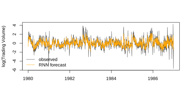
lab-r-nyse.svg.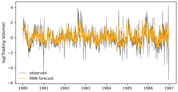
lab-py-nyse.svg.Notes on the book
Section 10.6: the relaxed lasso's test MAE of 224.8 is not reproduced
The book (p. 433) refits least squares on Hits, Walks, CRuns and PutOuts "to the training data (the so-called relaxed lasso)" and reports a test mean absolute error of 224.8. With the R lab's split (set.seed(13)) this model gives a test MAE of 234.70, in R and in Python. The split is certainly the book's: least squares on all predictors gives the book's 254.6687, and Table 10.3, fitted on the test players, is reproduced to every printed digit. The 224.8 may come from another set of four variables or from shrunken (lasso) coefficients; it is still the best of the methods compared, so the conclusion of the section stands.
Table 10.2: the \(R^2\) values look truncated, and the lasso keeps 13 variables with current glmnet
The test \(R^2\) of least squares is 0.5658 and that of the lasso 0.5182 (with the book's random folds); Table 10.2 prints 0.56 and 0.51, which are these numbers truncated rather than rounded (0.57 and 0.52). With glmnet 5.0 the book's call cv.glmnet(x[-testid, ], y[-testid], type.measure = "mae") after set.seed(13) gives a test MAE of 252.2981 (the book: 252.2994) and keeps 13 nonzero coefficients, not 12; the small differences come from changes in glmnet since the book was written.
Section 10.5.2: 4,276 training sequences, not 4,281
The book fits the RNN "using the 4,281 training sequences derived from the data before January 2, 1980". There are 4,281 training days, but the first five have no five-day history, so only 4,276 \((X,Y)\) pairs can be formed from them; with the 1,770 test pairs this makes the 6,046 pairs counted on p. 429 (4,281 + 1,770 = 6,051 is the number of days).
The two editions print different \(R^2\) for the same AR models
Not an error, but a source of confusion: the R lab prints 0.4132 and 0.4599, the Python lab 0.4129 and 0.4595 for the same least-squares fits, because R's var() divides by \(n-1\) and scikit-learn's score() by \(n\) (Filling the gap 10.8).
Footnote 23: what "\(d\) degrees of freedom" means for the natural splines
The footnote says that \(d\) degrees of freedom imply \(d\) knots at \(d\) quantiles of the data, and the text that the spline interpolates at \(d=n=20\). Both hold if \(d\) counts all basis functions, the constant included: a natural cubic spline with \(d\) knots (two of them boundary knots) spans a \(d\)-dimensional space (Result 7.3). With R's ns(x, df = d) plus an intercept, as in Chapter 7, there would be \(d+1\) parameters and interpolation at \(d=19\). The figures here use the first convention.
Typographical slips
p. 426: "the accompaying text" (accompanying); p. 440: "quite a bit less less wild" (one "less"); p. 441: "inbetween" (in between). The Python edition has the same three slips, on pp. 420, 433 and 434.
Exercises
Conceptual exercises 1–5 and applied exercises 6–13, in the book's numbering (the two editions have the same exercises, except that Exercise 13 of the Python edition varies the number of hidden units instead of the dictionary size). The applied solutions are the last sections of ch10_lab.R and ch10_lab.py; Exercises 8 and 13 need data that are not available here and are answered in words.
Exercise 10.1. A network has \(p=4\) inputs, two hidden layers with 2 and 3 units, and one output. (a) Draw it. (b) Write \(f(X)\) explicitly with ReLU activations. (c) Plug in some coefficients and compute \(f(X)\). (d) How many parameters does it have?
Solution
(a) Four input nodes \(X_1,\dots,X_4\), each joined to both units \(A^{(1)}_1,A^{(1)}_2\) of the first hidden layer; both joined to each of the three units \(A^{(2)}_1,A^{(2)}_2,A^{(2)}_3\) of the second; these three joined to the single output \(f(X)\): Figure 10.4 with 4, 2, 3 and 1 nodes.
(b)
\[ f(X)=\beta_0+\sum_{\ell=1}^3\beta_\ell\Big(w^{(2)}_{\ell0}+\sum_{k=1}^2w^{(2)}_{\ell k}\Big(w^{(1)}_{k0}+\sum_{j=1}^4w^{(1)}_{kj}X_j\Big)_+\Big)_+. \](c) Take \(A^{(1)}_1=(X_1+X_2-1)_+\), \(A^{(1)}_2=(X_3-X_4)_+\); \(A^{(2)}_1=(A^{(1)}_1+A^{(1)}_2)_+\), \(A^{(2)}_2=(A^{(1)}_1-A^{(1)}_2)_+\), \(A^{(2)}_3=(1-A^{(1)}_1)_+\); and \(f=1+2A^{(2)}_1-A^{(2)}_2+\frac12A^{(2)}_3\). At \(X=(1,2,4,1)\): \(A^{(1)}=(2,3)\), \(A^{(2)}=(5,0,0)\), so \(f(X)=1+10=11\). At \(X=(0,0,0,0)\): \(A^{(1)}=(0,0)\), \(A^{(2)}=(0,0,1)\), \(f=1.5\).
(d) By Filling the gap 10.2,
\[ (4+1)\cdot2+(2+1)\cdot3+(3+1)\cdot1=10+9+4=23. \]Exercise 10.2. (a) Show that adding a constant \(c\) to every \(Z_\ell\) in (10.13) leaves the probabilities unchanged. (b) In the multinomial logistic model (4.13), show that adding constants \(c_j\), \(j=0,\dots,p\), to the corresponding coefficients of every class leaves the predictions unchanged.
Solution
(a)
\[ \frac{e^{Z_m+c}}{\sum_\ell e^{Z_\ell+c}}=\frac{e^c\,e^{Z_m}}{e^c\sum_\ell e^{Z_\ell}}=\frac{e^{Z_m}}{\sum_\ell e^{Z_\ell}}. \](b) In (4.13) the class-\(k\) score is \(\eta_k(x)=\beta_{k0}+\sum_j\beta_{kj}x_j\). Replacing \(\beta_{kj}\) by \(\beta_{kj}+c_j\) for every class adds \(c_0+\sum_jc_jx_j\) to every score; at a fixed \(x\) this is the same constant for all classes, so by (a) the probabilities at \(x\) do not change. The model is therefore over-parametrised: one class's coefficients can be set to zero (as in the baseline form of Section 4.3.5), or a penalty or SGD picks one of the equivalent solutions. Checked numerically for random coefficients.
Exercise 10.3. Show that the negative multinomial log-likelihood (10.14) with \(M=2\) classes is minus the log of the likelihood (4.5).
Solution
With classes 0 and 1, \(y_{i1}=y_i\), \(y_{i0}=1-y_i\), \(f_1(x_i)=p(x_i)\) and \(f_0(x_i)=1-p(x_i)\). Then (10.14) is
\[ -\sum_i\big[y_i\log p(x_i)+(1-y_i)\log(1-p(x_i))\big]=-\log\prod_ip(x_i)^{y_i}(1-p(x_i))^{1-y_i}, \]and the product is the likelihood (4.5),
\[ \prod_{i:y_i=1}p(x_i)\prod_{i':y_{i'}=0}(1-p(x_{i'})). \]With softmax,
\[ p(x)=\frac{e^{Z_1}}{e^{Z_0}+e^{Z_1}}=\frac1{1+e^{-(Z_1-Z_0)}}, \]the logistic function of \(Z_1-Z_0\) (Result 10.4). See Filling the gap 10.3.
Exercise 10.4. A CNN takes 32 × 32 grey-scale images and has one convolution layer with three 5 × 5 filters, without padding. (a) Sketch the input and the first hidden layer. (b) How many parameters does it have? (c) Explain it as a feed-forward network with the pixels as inputs and constraints on the weights. (d) Without the constraints, how many weights would that network have?
Solution
(a) A 32 × 32 × 1 input; each filter fits in \(32-5+1=28\) positions in each direction, so the hidden layer is a 28 × 28 × 3 feature map (three channels).
(b) Each filter has 25 weights and a bias: \(3\times26=78\) parameters.
(c) Flatten the image into 1,024 inputs and the hidden layer into \(28\cdot28\cdot3=2{,}352\) units. Unit \((k,r,s)\) computes
\[ g\Big(b_k+\sum_{a,b}\text{filter}^{(k)}_{ab}\,x_{r+a-1,s+b-1}\Big): \]a dense unit whose weights are zero except on the 25 pixels of the 5 × 5 patch at \((r,s)\) (local connectivity), and whose 25 nonzero weights and bias are the same for all 784 units of channel \(k\) (weight sharing). See Filling the gap 10.4.
(d) \(1{,}024\times2{,}352=2{,}408{,}448\) weights, plus 2,352 biases: 2,410,800 parameters, about 31,000 times as many. The convolution demonstration computes both counts.
Exercise 10.5. In Table 10.2 the order of the three methods by mean absolute error differs from their order by test \(R^2\). How can this be?
Solution
The test \(R^2=1-\mathrm{MSE}/V\) is a decreasing function of the mean squared error (\(V\), the variance of the test responses, is the same for all methods), so ordering by \(R^2\) is ordering by MSE, a different criterion from the mean absolute error. Squaring weights large errors heavily: a method can have smaller errors on most players (smaller MAE) and a few larger misses on the highest salaries (larger MSE). In the book the lasso has the smallest MAE (252.3) but the smallest \(R^2\) (0.51); in our recomputation the lasso again has the smallest MAE (252.3) and the smallest \(R^2\) (0.522), with least squares the best by \(R^2\) (0.566). Salaries are skewed, with a few very high values, which makes the two criteria disagree easily; on 87 test players the differences are also well within sampling noise.
Exercise 10.6. Let \(R(\beta)=\sin\beta+\beta/10\). (a) Plot it on \([-6,6]\). (b) Find its derivative. (c) Run gradient descent with learning rate \(\rho=0.1\) from \(\beta^0=2.3\), showing the iterates. (d) Repeat from \(\beta^0=1.4\).
Solution
(b) \(R'(\beta)=\cos\beta+\frac1{10}\). Stationary points solve \(\cos\beta=-0.1\); minima also need \(R''(\beta)=-\sin\beta>0\), i.e. \(\sin\beta\lt0\): \(\beta=-\arccos(-0.1)+2\pi k\), that is \(\ldots,-1.6710,\ 4.6122,\ldots\)
R
# Exercise 6: gradient descent on R(beta) = sin(beta) + beta / 10 with learning rate 0.1
gd <- function(b0, rho = 0.1, tol = 1e-10, maxit = 10000) {
  b <- b0
  for (it in 1:maxit) {
    b_new <- b - rho * (cos(b) + 1 / 10)
    if (abs(b_new - b) < tol) break
    b <- b_new
  }
  c(beta = b_new, R = sin(b_new) + b_new / 10, steps = it)
}
ex6a <- gd(2.3); ex6b <- gd(1.4)
cat("Exercise 6: from 2.3 ->", round(ex6a, 6), "; from 1.4 ->", round(ex6b, 6), "\n")
Python
def gd(b, rho=0.1, tol=1e-10, maxit=10000):          # Exercise 6: R(beta) = sin(beta) + beta / 10
    for it in range(1, maxit + 1):
        b_new = b - rho * (np.cos(b) + 0.1)
        if abs(b_new - b) < tol:
            break
        b = b_new
    return b_new, np.sin(b_new) + b_new / 10, it

ex6a, ex6b = gd(2.3), gd(1.4)
print("Exercise 6: from 2.3 -> beta %.6f, R %.6f (%d steps); from 1.4 -> beta %.6f, R %.6f (%d steps)"
      % (ex6a + ex6b))
Exercise 6: from 2.3 -> 4.61222 -0.533765 217 ; from 1.4 -> -1.67096 -1.16208 227 Exercise 6: from 2.3 -> beta 4.612222, R -0.533765 (217 steps); from 1.4 -> beta -1.670964, R -1.162084 (227 steps)
(c) From 2.3 the gradient is negative (\(\cos2.3+0.1=-0.57\)), so the iterates move right, uphill of nothing, down into the minimum at \(\beta=4.6122\) with \(R=-0.5338\). (d) From 1.4 the gradient is positive (\(0.27\)), the iterates move left and end at the other minimum, \(\beta=-1.6710\), with \(R=-1.1621\), the lower of the two. The starting point decides which local minimum gradient descent finds, as in Figure 10.17.
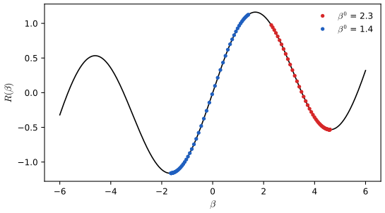
Exercise 6: the iterates from \(\beta^0=2.3\) (red) and \(\beta^0=1.4\) (blue), 60 steps each. Code: fig_ex6. Download: PDF · SVGExercise 10.7. Fit a network with one hidden layer of 10 units and dropout to the Default data, and compare its classification performance with logistic regression.
Solution
Inputs: student (0/1), balance and income, standardised; every third row is a test row (3,334 test, 6,666 training). The network has 10 ReLU units, 40% dropout and one logit output, fitted for 30 epochs.
R
# Exercise 7: Default data, one hidden layer of 10 units with dropout, against logistic regression
Xd <- scale(cbind(student = as.numeric(Default$student == "Yes"), balance = Default$balance, income = Default$income))
yd <- as.numeric(Default$default == "Yes")
te7 <- (seq_len(nrow(Default)) - 1) %% 3 == 0          # every third row is a test row
glm7 <- glm(yd ~ Xd, family = binomial, subset = !te7)
p_glm <- 1 / (1 + exp(-cbind(1, Xd[te7, ]) %*% coef(glm7)))
err_glm <- mean((p_glm > 0.5) != yd[te7])
set.seed(7)
nn7 <- fit_mlp(mlp_init(c(3, 10, 1)), Xd[!te7, ], yd[!te7], loss = "logit", epochs = 30, batch_size = 32,
               lr = 0.001, dropout = 0.4)$net
err_nn <- mean((predict_mlp(nn7, Xd[te7, ]) > 0) != yd[te7])
cat("Exercise 7: test error, logistic regression", err_glm, " network", err_nn, "\n")
Python
Default = common.isl_data("Default")                  # Exercise 7
Xd7 = np.column_stack([(Default["student"] == "Yes").astype(float), Default["balance"], Default["income"]])
Xd7 = (Xd7 - Xd7.mean(0)) / Xd7.std(0, ddof=1)
yd7 = (Default["default"] == "Yes").to_numpy(float)
te7 = np.arange(len(yd7)) % 3 == 0                    # every third row is a test row
glm7 = sm.GLM(yd7[~te7], sm.add_constant(Xd7[~te7]), family=sm.families.Binomial()).fit()
err_glm = np.mean((glm7.predict(sm.add_constant(Xd7[te7])) > 0.5) != yd7[te7])
torch.manual_seed(7)
nn7 = nn.Sequential(nn.Linear(3, 10), nn.ReLU(), nn.Dropout(0.4), nn.Linear(10, 1))
fit(nn7, tensor(Xd7[~te7]), tensor(yd7[~te7]), lambda o, t: nn.functional.binary_cross_entropy_with_logits(o.flatten(), t),
    epochs=30, batch_size=32, lr=0.001)
with torch.no_grad():
    err_nn = np.mean((nn7(tensor(Xd7[te7])).flatten().numpy() > 0) != yd7[te7])
print("Exercise 7: test error, logistic regression %.4f  network %.4f" % (err_glm, err_nn))
Exercise 7: test error, logistic regression 0.0278944 network 0.0314937 Exercise 7: test error, logistic regression 0.0279 network 0.0318
Logistic regression misclassifies 2.79% of the test customers in both languages; the network does no better (3.15% in R, 3.18% in Python). Only about 3% of customers default and the log-odds of default are close to linear in balance, so there is little nonlinearity for the network to find: another case for Occam's razor (Section 10.6). Both classifiers do barely better than predicting "no default" for everyone (3.3% error); a lower threshold than 0.5 would catch more defaulters, as in Section 4.4.2.
Exercise 10.8. Classify ten of your own photographs of animals with a pretrained CNN and report the top five classes and their probabilities.
Solution
This needs your photographs and the pretrained weights, so there is no fixed answer. Follow Section 10.9.4: crop each photograph so that the animal fills much of the frame (the hawk in Figure 10.10 is misclassified when it is small), resize to 224 × 224, apply ImageNet's normalisation, and take the five largest softmax probabilities. Expect confident, correct answers for common animals photographed clearly (dogs, cats, farm animals are well represented among the 1,000 ImageNet classes), confusions between similar breeds, and odd answers for unusual viewpoints. The probabilities are not calibrated against your own collection and should not be read as accuracy.
Exercise 10.9. Fit the lag-5 AR model to the NYSE data, then add a 12-level factor for the month. Does it help?
Solution
R
# Exercise 9: AR(5) with a 12-level month factor
arframem <- data.frame(month = factor(format(as.Date(NYSE$date[-(1:5)]), "%m")), arframe)
r2_m <- 1 - mean((predict(lm(log_volume ~ ., data = arframem[istrain, ]), arframem[!istrain, ]) -
                  arframe[!istrain, "log_volume"])^2) / V0
cat("Exercise 9: AR(5) + month: test R2", r2_m, " (without month", r2_ar, ")\n")
Python
month = pd.get_dummies(pd.to_datetime(NYSE["date"].iloc[5:]).dt.month, dtype=float).to_numpy()   # Exercise 9
r2_m = r2(ols_pred(np.column_stack([month[:, 1:], Xlag])))
print("Exercise 9: AR(5) + month: test R2 %.4f (without month %.4f)" % (r2_m, r2_ar))
Exercise 9: AR(5) + month: test R2 0.417042 (without month 0.413223 ) Exercise 9: AR(5) + month: test R2 0.4170 (without month 0.4132)
The test \(R^2\) rises from 0.4132 to 0.4170, identical in both languages: a small gain for 11 extra parameters, much less than the day of the week brings (0.4599). Trading volume has some seasonality (lower in late summer and around the holidays), but the 100-day moving-average normalisation of the volume series already removes much of it.
Exercise 10.10. Fit the linear AR model by flattening the short sequences prepared for the RNN, compare its test \(R^2\) with the lab's AR model, and discuss the two approaches.
Solution
R
# Exercise 10: a linear AR model from the flattened RNN input
xflat <- matrix(xrnn, n, 15)
r2_flat <- 1 - mean((cbind(1, xflat[!istrain, ]) %*% coef(lm(arframe[istrain, "log_volume"] ~ xflat[istrain, ])) -
                     arframe[!istrain, "log_volume"])^2) / V0
cat("Exercise 10: flattened linear AR: test R2", r2_flat, "\n")
Python
Xflat = X_rnn.reshape(len(yv), 15)                    # Exercise 10: the flattened RNN input
r2_flat = r2(ols_pred(Xflat))
print("Exercise 10: flattened linear AR: test R2 %.4f" % r2_flat)
Exercise 10: flattened linear AR: test R2 0.413223 Exercise 10: flattened linear AR: test R2 0.4132
The flattened array has the same 15 lagged columns as the AR design matrix, only in another order, so least squares gives exactly the same fit: \(R^2=0.4132\). Fitting the flattened input by a network with a single linear output layer (keras's
layer_flattenfollowed bylayer_dense(units = 1), as the book suggests) minimises the same criterion by SGD and would get close to, but not exactly, this solution, after many epochs. Advantages oflm(): exact, instantaneous, with standard errors and tests, and named lag variables. Advantages of the flattened tensor: the same data structure serves the RNN, the linear and the nonlinear AR models, so they are easy to compare and to extend (more layers, dropout).Exercise 10.11. Repeat Exercise 10 with a nonlinear AR model fitted to the flattened sequences.
Solution
R
# Exercise 11: a nonlinear AR model from the flattened input (no day of week)
set.seed(11)
nn11 <- fit_mlp(mlp_init(c(15, 32, 1)), xflat[istrain, ], arframe[istrain, "log_volume"], loss = "mse",
                epochs = 100, batch_size = 32, lr = 0.001, dropout = 0.5)$net
r2_11 <- 1 - mean((predict_mlp(nn11, xflat[!istrain, ]) - arframe[!istrain, "log_volume"])^2) / V0
cat("Exercise 11: flattened nonlinear AR: test R2", r2_11, "\n")
Python
torch.manual_seed(11)                                 # Exercise 11
nn11 = nn.Sequential(nn.Linear(15, 32), nn.ReLU(), nn.Dropout(0.5), nn.Linear(32, 1))
fit(nn11, tensor(Xflat[istrain]), Yr_tr, mse, epochs=100, batch_size=32, lr=0.001)
with torch.no_grad():
    r2_11 = r2(nn11(tensor(Xflat[~istrain])).flatten().numpy())
print("Exercise 11: flattened nonlinear AR: test R2 %.4f" % r2_11)
Exercise 11: flattened nonlinear AR: test R2 0.423128 Exercise 11: flattened nonlinear AR: test R2 0.4230
One hidden layer of 32 ReLU units with 50% dropout on the 15 flattened lags gives \(R^2\approx0.423\) in both languages, a little above the linear AR model (0.4132) and close to the book's 0.42 for its nonlinear AR model without the day of the week. Adding the day of the week matters more than the nonlinearity (0.468, Section 10.9.6).
Exercise 10.12. Include the day of the week in the RNN of Section 10.9.6 and compute the test \(R^2\).
Solution
The day of the week belongs to the target day \(t\), which is known when forecasting. One simple way to give it to the RNN is to append its five dummies to every element of the input sequence, so that each \(X_\ell\) has \(3+5=8\) components (another is to feed it into the output layer next to \(A_L\)).
R
# Exercise 12: the RNN with the day of week of the target day added to every step of the sequence
day <- model.matrix(~ day - 1, data = arframed)            # 5 dummies
xrnn_d <- array(0, c(n, 5, 8)); xrnn_d[, , 1:3] <- xrnn
for (l in 1:5) xrnn_d[, l, 4:8] <- day
set.seed(12)
rnn12 <- fit_rnn(rnn_init(8, 12), xrnn_d[istrain, , ], arframe[istrain, "log_volume"], epochs = 200, batch_size = 64)
r2_12 <- 1 - mean((rnn_forward(rnn12, xrnn_d[!istrain, , ])$out - arframe[!istrain, "log_volume"])^2) / V0
cat("Exercise 12: RNN + day of week: test R2", r2_12, "\n")
Python
X_rnn_d = np.concatenate([X_rnn, np.repeat(day[:, None, :], 5, axis=1)], axis=2)   # Exercise 12
torch.manual_seed(12)
rnn12 = NYSEModel(p=8)
fit(rnn12, tensor(X_rnn_d[istrain]), Yr_tr, mse, epochs=200, batch_size=64, lr=0.001)
with torch.no_grad():
    r2_12 = r2(rnn12(tensor(X_rnn_d[~istrain])).numpy())
print("Exercise 12: RNN + day of week: test R2 %.4f" % r2_12)
Exercise 12: RNN + day of week: test R2 0.456173 Exercise 12: RNN + day of week: test R2 0.4633
The test \(R^2\) rises from about 0.414 to 0.4562 and 0.4633 (R, Python), the same improvement as for the AR model (0.4132 to 0.4599) and in line with the book's statement that the RNN improves "to \(R^2=0.46\)" with the day of the week.
Exercise 10.13. Repeat the IMDb analysis of Section 10.9.5 with dictionaries of 1,000, 3,000, 5,000 and 10,000 words (R edition); or with 32 and 64 hidden units per layer, with and without 30% dropout (Python edition).
Solution
Not run here: the IMDb corpus is not available offline in this course. What to do: rebuild the binary bag-of-words matrix with the \(M\) most frequent words for each \(M\), fit the network of Section 10.9.5 (or the lasso path) on the 23,000 training reviews, choose the epoch (or \(\lambda\)) on the 2,000 validation reviews, and report test accuracy. What to expect: accuracy rises quickly with \(M\) and then levels off, because the most frequent sentiment words ("great", "worst", "boring", ...) are already among the first few thousand; most of the gain is reached by 3,000–5,000 words, and the extra rare words mostly add variance. For the Python edition's version, wider layers fit the training data faster and overfit sooner; 30% dropout slows the overfitting, and with the epoch chosen on the validation set all the variants end within about a percentage point of the 86–88% of the lab.
Demonstrations for this chapter
Each demonstration runs in the browser and links back to these notes. The ▶ Demo boxes above open them already set to the case under discussion.
| Demonstration | What you can see | Sections |
|---|---|---|
| A single-hidden-layer network on the Hitters data | The network of (10.1) trained in the browser by RMSprop with the gradients (10.29)–(10.30): training and test MAE by epoch against least squares and the lasso, and predicted against actual salaries. Presets: 1 full batch, no dropout; 2 the lab's network; 3 Table 10.2; 4 a big network trained too long; 5 one hidden unit. | 10.1, 10.6, 10.7, 10.9.1 |
| Convolution, ReLU and max pooling on a digit | Any 3 × 3 filter on an MNIST digit, the detector layer, two rounds of 2 × 2 pooling, a shift of the digit with the correlation of every map with the unshifted one, and a parameter counter for convolution against dense layers. Presets: 1 vertical stripe on a 1; 2 horizontal stripe on a 7; 3 an edge detector; 4 a one-pixel shift; 5 Exercise 4. | 10.3 |
| Double descent with minimum-norm natural splines | The natural-spline fit with any number \(d\) of basis functions, training and test error against \(d\), the size of the coefficients, five training samples, and ridge regression for comparison. Presets: 1 \(d=8\); 2 \(d=20\); 3 \(d=42\); 4 \(d=80\); 5 ridge. | 10.8 |
Related demonstrations in the companion courses: hidden units and weight decay and local connectivity and weight sharing in the ZIP code networks (Statistical Learning: Theory and Methods); backpropagation step by step, optimiser paths, dropout and ensembles, convolution arithmetic and the filters of a trained CNN (Foundations of Deep Learning).
References
- James, G., Witten, D., Hastie, T. and Tibshirani, R. (2021). An Introduction to Statistical Learning with Applications in R, 2nd edition. Springer, New York. Chapter 10, pp. 403–460. www.statlearning.com.
- James, G., Witten, D., Hastie, T., Tibshirani, R. and Taylor, J. (2023). An Introduction to Statistical Learning with Applications in Python. Springer, Cham. Chapter 10.
- Bishop, C. M. (1995). Training with noise is equivalent to Tikhonov regularization. Neural Computation, 7(1), 108–116.
- Belkin, M., Hsu, D., Ma, S. and Mandal, S. (2019). Reconciling modern machine-learning practice and the classical bias-variance trade-off. Proceedings of the National Academy of Sciences, 116(32), 15849–15854.
- Cybenko, G. (1989). Approximation by superpositions of a sigmoidal function. Mathematics of Control, Signals and Systems, 2, 303–314.
- He, K., Zhang, X., Ren, S. and Sun, J. (2016). Deep residual learning for image recognition. Proceedings of the IEEE Conference on Computer Vision and Pattern Recognition, 770–778.
- Hochreiter, S. and Schmidhuber, J. (1997). Long short-term memory. Neural Computation, 9(8), 1735–1780.
- Hornik, K., Stinchcombe, M. and White, H. (1989). Multilayer feedforward networks are universal approximators. Neural Networks, 2(5), 359–366.
- Krizhevsky, A. (2009). Learning Multiple Layers of Features from Tiny Images. Technical report.
- LeBaron, B. and Weigend, A. S. (1998). A bootstrap evaluation of the effect of data splitting on financial time series. IEEE Transactions on Neural Networks, 9(1), 213–220.
- LeCun, Y., Bottou, L., Bengio, Y. and Haffner, P. (1998). Gradient-based learning applied to document recognition. Proceedings of the IEEE, 86(11), 2278–2324.
- Maas, A. L., Daly, R. E., Pham, P. T., Huang, D., Ng, A. Y. and Potts, C. (2011). Learning word vectors for sentiment analysis. Proceedings of the 49th Annual Meeting of the Association for Computational Linguistics, 142–150.
- Rumelhart, D. E., Hinton, G. E. and Williams, R. J. (1986). Learning representations by back-propagating errors. Nature, 323, 533–536.
- Srivastava, N., Hinton, G., Krizhevsky, A., Sutskever, I. and Salakhutdinov, R. (2014). Dropout: a simple way to prevent neural networks from overfitting. Journal of Machine Learning Research, 15, 1929–1958.
- Tieleman, T. and Hinton, G. (2012). Lecture 6.5, RMSprop: divide the gradient by a running average of its recent magnitude. Neural Networks for Machine Learning (lecture notes).
The numerical statements in the text (the parameter counts, the convolution and pooling examples, the backpropagation formulas, the dropout and minimum-norm identities, the recomputed tables and figures, the agreement of the R and Python labs, and the demonstrations' numbers) were confirmed numerically.