Neural Networks
Take a few linear combinations of the inputs, pass each through a nonlinear function, and add the results: that one idea gives both projection pursuit regression, where the nonlinear functions are smooth curves estimated from the data, and the single-hidden-layer neural network, where they are rescaled and shifted copies of one fixed sigmoid. This chapter shows why such sums can approximate any continuous function, how both models are fitted (alternating smoothing and Gauss–Newton steps for projection pursuit; back-propagation and quasi-Newton methods for networks), why a network started near zero weights is almost linear and how weight decay keeps it from overfitting, how much the answer depends on the random start and why one should average predictions rather than weights, how local connectivity and weight sharing turned a generic network into a good digit recogniser, and what made Bayesian networks win a feature-selection challenge.
Ch. 1 Introduction Ch. 2 Supervised learning Ch. 3 Linear regression Ch. 4 Linear classification Ch. 5 Basis expansions Ch. 6 Kernel smoothing Ch. 7 Model assessment Ch. 8 Inference and averaging Ch. 9 Additive models and trees Ch. 10 Boosting Ch. 11 Neural networks Ch. 12 SVMs Ch. 13 Nearest neighbours Ch. 14 Unsupervised learning Ch. 15 Random forests Ch. 16 Ensembles Ch. 17 Graphical models Ch. 18 High-dimensional problems
How to read these notes
They follow the book. Sections carry the book's numbers (11.1, 11.5.2, ...) and every displayed equation that appears in the book carries the book's own equation number, e.g. \((11.15)\), so you can read these notes next to the book. Equations without a number are steps that the book skips.
Filling the gaps. Wherever the book states a result without proof, leaves it to an exercise, or describes an algorithm without deriving it, an orange Filling the gap box or a proof gives the full argument. Proofs and derivations start hidden: open one with its bar, or use the button below.
Figures and demonstrations. Every figure of the chapter that is computed from data or a model is reproduced from scratch by the Python code. Figures 11.2 and 11.10 are diagrams; Figure 11.12 reports competition results that cannot be rerun here and is replaced by a CPU-scale version of the same comparison. Seven supplementary figures (11.S1–11.S7) illustrate points the book makes in words and the computational exercises. The ▶ Demo boxes open an interactive demonstration already set to the case being discussed.
Main reference
T. Hastie, R. Tibshirani and J. Friedman, The Elements of Statistical Learning: Data Mining, Inference, and Prediction, 2nd edition, Springer (2009), Chapter 11, pages 389–416 (book website, with the data sets: hastie.su.domains/ElemStatLearn). Section, equation, figure and exercise numbers below refer to this book. Further reading is listed in the references.
The explanations, derivations, figures and code are my own; equations are cited by their numbers in the book.
Companion courses
Most of the network material of this chapter is treated at length in the two companion courses on this site. The overlapping material is:
- Section 11.3 (the network, universal approximation, symmetries of the weights): Foundations of Deep Learning, Section 6.2, with Result 6.2 and Result 6.4; Bayesian and Probabilistic Machine Learning, Section 5.1, with Result 5.1 and Result 5.2.
- Section 11.4 (error functions, back-propagation, gradient descent, stochastic approximation): Foundations of Deep Learning, Section 8.1 (Result 8.1, Result 8.2), Section 7.2 and Result 7.9; Bayesian and Probabilistic Machine Learning, Section 5.3 (Result 5.6).
- Section 11.5 (initialisation, early stopping, weight decay, input normalisation, model averaging): Foundations of Deep Learning, Section 7.2.5, Section 7.4.1, Section 9.2, Section 9.3.1, Section 9.6; Bayesian and Probabilistic Machine Learning, Section 5.5.
- Section 11.7 (local connectivity, weight sharing, convolutional networks): Foundations of Deep Learning, Section 10.2 and Section 9.4; Bayesian and Probabilistic Machine Learning, Section 5.5.6.
- Section 11.9 (Bayesian networks, hybrid Monte Carlo, committees and boosting): Bayesian and Probabilistic Machine Learning, Section 5.7, Section 11.5.2 and Section 14.2.
Where a proof there is the same, these notes state the result, sketch the argument and link to it. New here: projection pursuit regression (the Gauss–Newton step, a complete proof that sums of ridge functions are universal approximators, the polarisation identity for products), back-propagation in the book's notation with the biases restored, the weight-elimination penalty, the near-linearity of a network with small weights with an explicit cubic error bound, the simulated examples with their exact signal variances, the parameter counts of the ZIP code networks, the standard errors of compared error rates, the Gibbs step behind automatic relevance determination, and several corrections to the book (the weight-decay gradient, the missing biases in (11.12), the weight-elimination penalty, the scale of the radial example, two slips in Section 11.9.1).
The chapter at a glance
- 11.2 Projection pursuit regression (PPR) fits \(f(x)=\sum_mg_m(\omega_m^\T x)\) (Definition 11.1); products of inputs are sums of ridge functions (Result 11.1) and so is, approximately, every continuous function (Result 11.2); each direction is updated by a Gauss–Newton step that is a weighted least-squares fit (Filling the gap 11.1).
- 11.3 A single-hidden-layer network is a PPR model whose ridge functions are scaled and shifted sigmoids (Result 11.3), it is a universal approximator too (Result 11.4), and its weights are never identifiable (Filling the gap 11.2).
- 11.4 Back-propagation computes all derivatives in two passes (Result 11.5); softmax with cross-entropy gives the output errors \(f_k-y_k\) (Result 11.6).
- 11.5 With weights near zero the network is linear up to a cubic error (Result 11.7), exactly zero weights never move apart (Filling the gap 11.5); weight decay is ridge regression for networks (Filling the gap 11.6); averaging the predictions of several starts never hurts, averaging their weights can be disastrous (Result 11.9).
- 11.6 The sum of sigmoids is the ideal case for a network and the radial function the worst (Result 11.10; Figures 11.6–11.8).
- 11.7 Local connectivity and weight sharing cut the number of weights from 3214 to 1060 while raising the number of links to 5194 (Result 11.11); the gradient for a shared weight is the sum of the gradients of its links (Result 11.12).
- 11.9 Bayesian networks average over the posterior, bagging over bootstrap samples, boosting over a sequence of fits (11.21); hybrid Monte Carlo and Gibbs steps for the ARD precisions make the posterior computable (Result 11.13, Filling the gap 11.9).
Notation. Inputs \(x\in\R^p\), training pairs \((x_i,y_i)\), \(i=1,\dots,N\); for \(K\) outputs \(y_{ik}\), \(k=1,\dots,K\) (one-hot class indicators for classification). The logistic sigmoid is \(\sigma(v)=1/(1+e^{-v})\), with \(\sigma'(v)=\sigma(v)(1-\sigma(v))\). Hidden units \(z_{mi}=\sigma(\alpha_{0m}+\alpha_m^\T x_i)\), \(m=1,\dots,M\); output activations \(T_{ki}=\beta_{0k}+\beta_k^\T z_i\); outputs \(f_k(x_i)=g_k(T_i)\). \(\theta\) collects all weights, \(R(\theta)\) is the error, \(J(\theta)\) the penalty and \(\lambda\ge0\) the weight decay.
Prerequisites. Least squares and ridge regression (Section 3.4.1), multinomial logistic regression (Section 4.4), smoothing splines (Section 5.4), the chain rule, Taylor's theorem and the Weierstrass approximation theorem.
11.1 Introduction
p. 389 Statistics and artificial intelligence arrived, independently, at the same kind of model: form a few linear combinations of the inputs ("derived features") and model the response as a nonlinear function of them. The statistical version, projection pursuit regression, came out of semiparametric smoothing; the neural network came out of models of the brain. The chapter treats the first briefly and the second at length; the theme throughout is that a neural network is a nonlinear statistical model, fitted by (penalised) least squares or maximum likelihood, and subject to all the usual concerns about overfitting.
11.2 Projection Pursuit Regression
pp. 389–392
Definition 11.1 (projection pursuit regression; ridge functions) p. 389, (11.1)
Let \(\omega_1,\dots,\omega_M\) be unit vectors in \(\R^p\) and \(g_1,\dots,g_M\) functions from \(\R\) to \(\R\). The projection pursuit regression (PPR) model is
\[ f(X)=\sum_{m=1}^Mg_m(\omega_m^\T X). \tag{11.1} \]A function of the form \(x\mapsto g(\omega^\T x)\) is a ridge function: it is constant on every hyperplane orthogonal to \(\omega\) and varies only along \(\omega\). PPR is an additive model in the derived features \(V_m=\omega_m^\T X\) rather than in the inputs; both the directions and the functions are estimated. The case \(M=1\) is the single index model of econometrics.
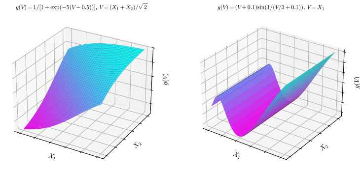
fig_11_1. Reproduces Hastie, Tibshirani and Friedman (2009), Figure 11.1. Download: PDF · SVGSums of ridge functions are far richer than they look. The book's example is the product of two inputs, and the same trick works for any monomial.
Result 11.1 (products are sums of ridge functions) p. 390
For all \(x\in\R^p\),
\[ x_1x_2=\tfrac14\big[(x_1+x_2)^2-(x_1-x_2)^2\big], \]a sum of two ridge functions with directions \((1,\pm1,0,\dots,0)^\T/\sqrt2\) and quadratic \(g\)'s. More generally (polarisation) for \(d\) coordinates
\[ x_1x_2\cdots x_d=\frac1{2^d\,d!}\sum_{\varepsilon\in\{-1,1\}^d}\varepsilon_1\varepsilon_2\cdots\varepsilon_d\,(\varepsilon_1x_1+\cdots+\varepsilon_dx_d)^d, \]a sum of \(2^d\) (or, pairing \(\varepsilon\) with \(-\varepsilon\), \(2^{d-1}\)) ridge functions of the form \(c\,v^d\).
Proof
The first identity is \((a+b)^2-(a-b)^2=4ab\). For the second, expand \((\sum_j\varepsilon_jx_j)^d\) by the multinomial theorem: it is \(\sum_{|k|=d}\binom{d}{k}\prod_j\varepsilon_j^{k_j}x_j^{k_j}\) over multi-indices \(k=(k_1,\dots,k_d)\). Multiply by \(\prod_j\varepsilon_j\) and sum over \(\varepsilon\): the coefficient of \(\prod_jx_j^{k_j}\) becomes \(\binom dk\prod_j\big(\sum_{\varepsilon_j=\pm1}\varepsilon_j^{k_j+1}\big)\). The inner sum is 2 when \(k_j+1\) is even and 0 when it is odd, so only multi-indices with every \(k_j\) odd survive; with \(\sum_jk_j=d\) and \(d\) coordinates, every \(k_j\ge1\) forces \(k=(1,\dots,1)\). That term has coefficient \(\binom{d}{1,\dots,1}2^d=d!\,2^d\). Dividing by \(2^dd!\) gives the identity. Replacing \(\varepsilon\) by \(-\varepsilon\) multiplies both \(\prod_j\varepsilon_j\) and \((\sum_j\varepsilon_jx_j)^d\) by \((-1)^d\), so the two terms are equal and pair up. ∎
The book then states that with \(M\) large enough PPR approximates any continuous function on \(\R^p\) arbitrarily well, a universal approximator. Here is a complete proof.
Result 11.2 (sums of ridge functions are dense) p. 390
Let \(K\subset\R^p\) be compact and \(f:K\to\R\) continuous. For every \(\epsilon>0\) there are \(M\), unit vectors \(\omega_1,\dots,\omega_M\) and polynomials \(g_1,\dots,g_M\) of one variable with
\[ \sup_{x\in K}\Big|f(x)-\sum_{m=1}^Mg_m(\omega_m^\T x)\Big|\lt \epsilon. \]In fact every polynomial of degree \(D\) in \(p\) variables is exactly a finite sum of ridge polynomials.
Proof
Step 1 (Weierstrass). By the Stone–Weierstrass theorem there is a polynomial \(P\) with \(\sup_K|f-P|\lt \epsilon\). It suffices to write \(P\) exactly as a finite sum of ridge functions.
Step 2 (reduce to homogeneous parts). \(P=\sum_{d=0}^DP_d\) with \(P_d\) homogeneous of degree \(d\). Let \(\mathcal H_d\) be the space of homogeneous polynomials of degree \(d\) in \(p\) variables, a finite-dimensional vector space, and \(\mathcal R_d\subseteq\mathcal H_d\) the span of the powers \((a^\T x)^d\), \(a\in\R^p\). If \(\mathcal R_d=\mathcal H_d\), then each \(P_d\) is a finite combination \(\sum_jc_j(a_j^\T x)^d=\sum_j c_j\|a_j\|^d(\omega_j^\T x)^d\) with \(\omega_j=a_j/\|a_j\|\), a sum of ridge functions, and so is \(P\).
Step 3 (the powers span). On \(\mathcal H_d\) use the inner product \(\langle q,r\rangle=q(\partial)\,r\), where \(q(\partial)\) replaces each \(x_j\) by \(\partial/\partial x_j\). On monomials, \(\langle x^k,x^l\rangle=k!\) if \(k=l\) and 0 otherwise (\(k!=\prod_jk_j!\)), so this is a genuine inner product (positive definite, with the monomials orthogonal). For \(r(x)=(a^\T x)^d\), \(\partial^k(a^\T x)^d=d!\,a^k\) for \(|k|=d\) (differentiate \(d\) times; each derivative in \(x_j\) brings down a factor \(a_j\)). Hence for \(q=\sum_kq_kx^k\),
\[ \langle q,(a^\T x)^d\rangle=\sum_{|k|=d}q_k\,d!\,a^k=d!\;q(a). \]If \(q\in\mathcal H_d\) is orthogonal to \(\mathcal R_d\), then \(q(a)=0\) for every \(a\in\R^p\), so \(q\) is the zero polynomial. The orthogonal complement of \(\mathcal R_d\) in the finite-dimensional space \(\mathcal H_d\) is therefore \(\{0\}\), and \(\mathcal R_d=\mathcal H_d\). (A spanning set needs at most \(\dim\mathcal H_d=\binom{p+d-1}{d}\) directions.)
Combining the steps, \(P(x)=\sum_mg_m(\omega_m^\T x)\) with polynomial \(g_m\) (group the terms with the same direction), and \(\sup_K|f-\sum_mg_m(\omega_m^\T\cdot)|\lt \epsilon\). ∎
The generality has a price: each input enters through every term, in a different nonlinear way, so a fitted PPR model is hard to interpret. It is a tool for prediction; the single index model is the exception, being only slightly more general than linear regression.
Fitting. Given data, we seek approximate minimisers of
\[ \sum_{i=1}^N\Big[y_i-\sum_{m=1}^Mg_m(\omega_m^\T x_i)\Big]^2 \tag{11.2} \]over the functions and the directions, with complexity constraints on the \(g_m\) (otherwise \(g_m\) could interpolate the data). With one term and a fixed \(\omega\), the derived values \(v_i=\omega^\T x_i\) turn the problem into one-dimensional smoothing: any scatterplot smoother, for instance a smoothing spline (Section 5.4), estimates \(g\). With \(g\) fixed, \(\omega\) is updated by a Gauss–Newton step: linearise \(g\) around the current direction,
\[ g(\omega^\T x_i)\approx g(\omega_{\rm old}^\T x_i)+g'(\omega_{\rm old}^\T x_i)(\omega-\omega_{\rm old})^\T x_i, \tag{11.3} \]which gives
\[ \sum_{i=1}^N\big[y_i-g(\omega^\T x_i)\big]^2\approx\sum_{i=1}^Ng'(\omega_{\rm old}^\T x_i)^2\bigg[\Big(\omega_{\rm old}^\T x_i+\frac{y_i-g(\omega_{\rm old}^\T x_i)}{g'(\omega_{\rm old}^\T x_i)}\Big)-\omega^\T x_i\bigg]^2. \tag{11.4} \]The right side is minimised by a weighted least-squares regression, without intercept, of the working response \(\omega_{\rm old}^\T x_i+(y_i-g(\omega_{\rm old}^\T x_i))/g'(\omega_{\rm old}^\T x_i)\) on \(x_i\) with weights \(g'(\omega_{\rm old}^\T x_i)^2\). The two steps are repeated until the fit stops improving.
Filling the gap 11.1: why (11.4) is a Gauss–Newton step, and why it goes downhill p. 391
Derivation
The algebra of (11.4). Write \(v_i=\omega_{\rm old}^\T x_i\), \(r_i=y_i-g(v_i)\), \(d_i=g'(v_i)\). Substituting (11.3), the \(i\)-th residual is \[ y_i-g(\omega^\T x_i)\approx r_i-d_i(\omega-\omega_{\rm old})^\T x_i=r_i+d_iv_i-d_i\,\omega^\T x_i \]. Its square is \(d_i^2\big[(v_i+r_i/d_i)-\omega^\T x_i\big]^2\) whenever \(d_i\ne0\), which is (11.4). To avoid dividing by small \(d_i\), the code minimises the equivalent form \(\sum_i(r_i+d_iv_i-d_i\,x_i^\T\omega)^2\), an ordinary least-squares regression of \(r_i+d_iv_i\) on the rows \(d_ix_i^\T\): with \(\mathbf D=\diag(d_i)\),
\[ \omega_{\rm new}=(\bX^\T\mathbf D^2\bX)^{-1}\bX^\T\mathbf D(\mathbf Dv+\br). \]Gauss–Newton. Let \(S(\omega)=\sum_i\rho_i(\omega)^2\) with \(\rho_i(\omega)=y_i-g(\omega^\T x_i)\). Its gradient is \(\nabla S=-2\bJ^\T\rho\), where the Jacobian of \(g(\omega^\T x_i)\) has rows \(\bJ_i=d_ix_i^\T\), i.e. \(\bJ=\mathbf D\bX\). Its Hessian is \(2\bJ^\T\bJ-2\sum_i\rho_i\,g''(v_i)\,x_ix_i^\T\). Newton's method uses both terms; Gauss–Newton drops the second, which involves \(g''\) and is small when the residuals are small. The Gauss–Newton step solves \(\bJ^\T\bJ\,\Delta=\bJ^\T\rho\), i.e. \(\bX^\T\mathbf D^2\bX\,\Delta=\bX^\T\mathbf D\br\), and \(\omega_{\rm old}+\Delta\) is exactly the \(\omega_{\rm new}\) above (since \(\bX^\T\mathbf D^2\bX\,\omega_{\rm old}=\bX^\T\mathbf D^2v\)).
It is a descent direction. If \(\bJ^\T\bJ\) is positive definite, \(\nabla S^\T\Delta=-2\rho^\T\bJ(\bJ^\T\bJ)^{-1}\bJ^\T\rho\le0\), with equality only when \(\bJ^\T\rho=0\) (a stationary point). So a small enough step along \(\Delta\) reduces \(S\) for fixed \(g\); the code halves the step until the criterion, recomputed with the smoother refitted on the new projections, decreases.
Why \(\omega\) can be renormalised. For fixed data, \(g(\omega^\T x)\) with \(\omega=c\,u\), \(\|u\|=1\), equals \(\tilde g(u^\T x)\) with \(\tilde g(v)=g(cv)\), and the smoothing step re-estimates \(g\) anyway; so after each update the direction is divided by its length (and its sign fixed, since \(g(\omega^\T x)=h(-\omega^\T x)\) with \(h(v)=g(-v)\)). ∎
With several terms the model is built forward stagewise, adding one pair \((\omega_m,g_m)\) at a time fitted to the residuals of the previous terms. Implementation details (p. 391): a smoother that provides derivatives is convenient (local regression or smoothing splines); after each new term the earlier \(g_m\) may be readjusted by backfitting (Chapter 9), usually leaving the \(\omega_m\) fixed; and the number of terms is chosen by stopping when a new term does not improve the fit appreciably, or by cross-validation. The book also notes that projection pursuit ideas apply to density estimation and to independent component analysis (Section 14.7), and that the computational cost of PPR in 1981 explains why statisticians used it little.
The fitting procedure used in these notes (one possible implementation)
- Set \(\hat c=\bar y\) and the current fit to 0. For \(m=1,\dots,M\): let \(r_i=y_i-\hat c-\sum_{j\lt m}\hat g_j(\hat\omega_j^\T x_i)\).
- From each starting direction (the least-squares direction of \(r\) on \(x\), and a few fixed directions), alternate: (a) smooth \(r_i\) against \(v_i=\omega^\T x_i\) with a cubic smoothing spline of fixed degrees of freedom, centred over the data; (b) the Gauss–Newton step of Filling the gap 11.1, halving it until the residual sum of squares decreases; stop when the relative decrease is below \(10^{-8}\). Keep the start with the smallest residual sum of squares.
- Backfit \(\hat g_1,\dots,\hat g_m\) with the directions fixed: cycle through \(j\), re-smoothing the partial residuals \(y_i-\hat c-\sum_{l\ne j}\hat g_l(\hat\omega_l^\T x_i)\) against \(\hat\omega_j^\T x_i\), until the fits stop changing.
The spline is a cubic B-spline basis with ten interior knots at equally spaced ranks of \(v\) and the penalty \(\lambda\int g''(v)^2\d v\) (a smoothing spline on a reduced knot set), with \(\lambda\) chosen so that the trace of the smoother equals the requested degrees of freedom, as in Section 5.4; the derivative \(g'\) comes from the basis. Code: RidgeSmoother, ppr_single, ppr_fit.
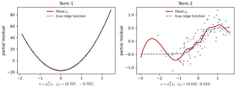
fig_11_s2.11.3 Neural Networks
pp. 392–395 The "vanilla" network of the chapter is the single-hidden-layer, feed-forward network, also called the single hidden layer back-propagation network or single layer perceptron. Figure 11.2 of the book is its diagram (inputs at the bottom, \(M\) hidden units in the middle, \(K\) outputs on top, every unit connected to every unit in the next layer; it is not reproduced). It handles regression (usually \(K=1\)) and \(K\)-class classification (one output per class) in the same way.
See also (companion courses): Foundations of Deep Learning, Section 6.2 and Bayesian and Probabilistic Machine Learning, Section 5.1.
Definition 11.2 (single-hidden-layer network) p. 392, (11.5)–(11.6)
\[ \begin{aligned} Z_m&=\sigma(\alpha_{0m}+\alpha_m^\T X),\quad m=1,\dots,M,\\ T_k&=\beta_{0k}+\beta_k^\T Z,\quad k=1,\dots,K,\\ f_k(X)&=g_k(T),\quad k=1,\dots,K, \end{aligned} \tag{11.5} \]with \(Z=(Z_1,\dots,Z_M)\), \(T=(T_1,\dots,T_K)\) and activation \(\sigma\), usually the sigmoid \(\sigma(v)=1/(1+e^{-v})\). The output function is the identity \(g_k(T)=T_k\) for regression; for classification it is the softmax
\[ g_k(T)=\frac{e^{T_k}}{\sum_{\ell=1}^Ke^{T_\ell}}, \tag{11.6} \]the transformation of the multiple logistic model (Section 4.4), which gives positive estimates that sum to one. The \(Z_m\) are hidden units; the intercepts \(\alpha_{0m},\beta_{0k}\) are often drawn as a bias unit, a constant input 1 feeding every unit. With Gaussian radial functions in place of \(\sigma\) one obtains a radial basis function network (Section 6.7).
Early classification networks used the identity output too; the book notes that this was abandoned for the softmax, and recalls the masking problem of linear outputs (Section 4.2). The hidden units are a basis expansion of the inputs, \(h_m(X)=Z_m\), and the network is a linear (or linear logistic) model in them; the difference from Chapter 5 is that the parameters of the basis functions are learned from the data.
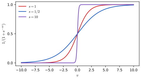
fig_11_3. Reproduces Hastie, Tibshirani and Friedman (2009), Figure 11.3. Download: PDF · SVGTwo remarks of the book are worth making precise. If \(\sigma\) is the identity, every \(T_k\) is an affine function of \(X\) (a composition of affine maps), so the network collapses to a linear model: the nonlinearity is what enlarges the class. And if \(\|\alpha_m\|\) is small, unit \(m\) operates in the nearly linear middle part of the sigmoid (Result 11.7). Finally, the one-hidden-layer network is a PPR model:
Result 11.3 (a network is projection pursuit with sigmoidal ridge functions; Exercise 11.1) p. 394, (11.7)
For a regression network (\(K=1\), identity output) with \(\alpha_m\ne0\), put \(s_m=\|\alpha_m\|\) and \(\omega_m=\alpha_m/s_m\). Then
\[ \begin{aligned} g_m(\omega_m^\T X)&=\beta_m\sigma(\alpha_{0m}+\alpha_m^\T X)\\ &=\beta_m\sigma(\alpha_{0m}+\|\alpha_m\|(\omega_m^\T X)), \end{aligned} \tag{11.7} \]so \(f(X)=\beta_0+\sum_mg_m(\omega_m^\T X)\) is a PPR model (11.1) whose ridge functions belong to the three-parameter family \(\sigma_{\beta,\alpha_0,s}(v)=\beta\sigma(\alpha_0+sv)\) (the constant \(\beta_0\) can be absorbed into any \(g_m\)). A unit with \(\alpha_m=0\) contributes the constant \(\beta_m\sigma(\alpha_{0m})\). For \(K\) outputs, every output \(T_k=\beta_{0k}+\sum_m\beta_{km}\sigma(\alpha_{0m}+s_m\omega_m^\T X)\) is a PPR model with the same directions and the same unit shapes but its own scales \(\beta_{km}\): a multiple-response PPR model with shared directions, followed by the output transformation \(g_k\).
Proof
\(\alpha_m^\T X=\|\alpha_m\|\,(\alpha_m/\|\alpha_m\|)^\T X=s_m\,\omega_m^\T X\), and substituting into \(T=\beta_0+\sum_m\beta_m\sigma(\alpha_{0m}+\alpha_m^\T X)\) gives (11.7) term by term. Conversely, any PPR model whose ridge functions are of the form \(\beta\sigma(\alpha_0+sv)\) is a network with \(\alpha_m=s_m\omega_m\). The multi-output case is the same computation for each \(k\). ∎
Because \(\beta\sigma(\alpha_0+sv)\) is much less flexible than a nonparametric \(g\), a network typically uses 20 or 100 units where PPR uses 5 or 10 terms. Yet a network is still a universal approximator.
Result 11.4 (universal approximation by one hidden layer)
Let \(\sigma\) be continuous with \(\sigma(v)\to0\) as \(v\to-\infty\) and \(\sigma(v)\to1\) as \(v\to\infty\). For every continuous \(f\) on a compact \(K\subset\R^p\) and \(\epsilon>0\) there is a network \(\beta_0+\sum_{m=1}^M\beta_m\sigma(\alpha_{0m}+\alpha_m^\T x)\) within \(\epsilon\) of \(f\) uniformly on \(K\).
Proof (from Result 11.2)
By Result 11.2, \(\sup_K|f-\sum_{j=1}^Jg_j(\omega_j^\T x)|\lt \epsilon/2\) with continuous \(g_j\). Each \(v_j=\omega_j^\T x\) ranges over a compact interval \([a,b]\) (containing all of them). It is enough to show that each continuous \(g\) on \([a,b]\) is within \(\epsilon/(2J)\) of a sum \(c_0+\sum_l c_l\sigma(s(v-t_l))\), because \(s(\omega_j^\T x-t_l)=\alpha_0+\alpha^\T x\) with \(\alpha=s\omega_j\), \(\alpha_0=-st_l\), and summing over \(j\) gives a network.
Staircase. \(g\) is uniformly continuous on \([a,b]\): given \(\eta>0\) choose \(n\) so that \(|g(u)-g(v)|\lt \eta\) whenever \(|u-v|\le h=(b-a)/n\). Put \(t_l=a+lh\), jump points \(c_l=t_l-h/2\) and jumps \(J_l=g(t_l)-g(t_{l-1})\), so \(|J_l|\lt \eta\), for \(l=1,\dots,n\). With \(H\) the unit step, \(G(v)=g(t_0)+\sum_{l=1}^nJ_lH(v-c_l)\) equals \(g(t_L)\) on \([c_L,c_{L+1})\) (telescoping), and every \(v\) there is within \(h/2\) of \(t_L\); hence \(|g-G|\lt \eta\) on \([a,b]\).
Smoothing the steps. Let \(S(v)=g(t_0)+\sum_lJ_l\,\sigma(s(v-c_l))\). Put \(B=\sup_u|\sigma(u)-H(u)|\), finite because \(\sigma\) is continuous with finite limits, and \(e(r)=\sup_{|u|\ge r}|\sigma(u)-H(u)|\), which tends to 0 as \(r\to\infty\). The jump points are \(h\) apart, so any \(v\) is within \(\delta=h/4\) of at most one of them; that term contributes at most \(|J_l|B\lt B\eta\), and each of the other (at most \(n\)) terms at most \(\eta\,e(s\delta)\). So \(|g-S|\le\eta+B\eta+n\eta\,e(s\delta)\) on \([a,b]\). Choose \(\eta\) with \((2+B)\eta\lt \epsilon/(2J)\), which fixes \(n\) and \(\delta\), and then \(s\) so large that \(n\,e(s\delta)\lt1\). Then \(|g-S|\lt \epsilon/(2J)\). ∎
The companion courses state the general theorem (one hidden layer with any non-polynomial activation is dense) and discuss its meaning: Foundations of Deep Learning, Result 6.2; Bayesian and Probabilistic Machine Learning, Result 5.1.
Filling the gap 11.2: the weights of a network are never identifiable pp. 394, 408
Many weight vectors give the same function, which matters for interpretation (Section 11.8) and for averaging (Section 11.5.5).
Derivation
Permutations. Relabelling the hidden units, i.e. permuting the pairs \((\alpha_{0m},\alpha_m)\) and the columns \(\beta_{\cdot m}\) together, leaves every \(T_k\) unchanged: \(M!\) equivalent weight vectors.
Sign flips. The sigmoid satisfies \(\sigma(-v)=1-\sigma(v)\) (multiply numerator and denominator of \(1/(1+e^{v})\) by \(e^{-v}\)). Hence \[ \beta_{km}\sigma(\alpha_{0m}+\alpha_m^\T x)=\beta_{km}-\beta_{km}\sigma(-\alpha_{0m}-\alpha_m^\T x) \]: replacing \((\alpha_{0m},\alpha_m,\beta_{km})\) by \((-\alpha_{0m},-\alpha_m,-\beta_{km})\) and \(\beta_{0k}\) by \(\beta_{0k}+\beta_{km}\) gives the same outputs. With the \(M!\) permutations this makes \(2^MM!\) equivalent points for a generic network.
Degenerate units. If \(\beta_{\cdot m}=0\), the weights \(\alpha_m\) are arbitrary; if \(\alpha_m=0\), the unit is a constant that trades off with \(\beta_{0k}\); two units with equal \((\alpha_{0m},\alpha_m)\) only identify the sum of their output weights. With softmax outputs, adding the same vector to every \((\beta_{0k},\beta_k)\) leaves (11.6) unchanged.
The same symmetries for tanh units are in Bayesian and Probabilistic Machine Learning, Result 5.2 and Foundations of Deep Learning, Result 6.4. ∎
The name "neural network" comes from the first models of the brain: units are neurons, links are synapses, and a neuron fires (a step function in place of \(\sigma\) and \(g_k\)) when its input exceeds a threshold. For statistical fitting a step is not smooth enough to optimise, and it was replaced by the sigmoid.
11.4 Fitting Neural Networks
pp. 395–397 The unknown weights \(\theta\) are
\[ \begin{aligned} &\{\alpha_{0m},\alpha_m;\ m=1,2,\dots,M\}&&M(p+1)\text{ weights},\\ &\{\beta_{0k},\beta_k;\ k=1,2,\dots,K\}&&K(M+1)\text{ weights}. \end{aligned} \tag{11.8} \]For regression the error is the residual sum of squares,
\[ R(\theta)=\sum_{k=1}^K\sum_{i=1}^N(y_{ik}-f_k(x_i))^2, \tag{11.9} \]and for classification either squared error or the cross-entropy (deviance)
\[ R(\theta)=-\sum_{i=1}^N\sum_{k=1}^Ky_{ik}\log f_k(x_i), \tag{11.10} \]with classifier \(G(x)=\argmax_kf_k(x)\). With the softmax and the cross-entropy, the network is a linear logistic regression in the hidden units and all parameters are estimated by maximum likelihood (Result 11.6). The global minimiser of \(R\) is usually an overfit; regularisation comes from a penalty or from early stopping (Section 11.5). The basic method of fitting is gradient descent, called back-propagation here because of how the gradient is computed.
See also (companion courses): Foundations of Deep Learning, Section 8.1 (back-propagation for any feed-forward network, its cost, gradient checking); Bayesian and Probabilistic Machine Learning, Section 5.3.
For squared error write \(z_{mi}=\sigma(\alpha_{0m}+\alpha_m^\T x_i)\), \(z_i=(z_{1i},\dots,z_{Mi})\) and
\[ R(\theta)\equiv\sum_{i=1}^NR_i=\sum_{i=1}^N\sum_{k=1}^K(y_{ik}-f_k(x_i))^2. \tag{11.11} \]Result 11.5 (back-propagation for squared error) pp. 395–396, (11.12)–(11.15)
Suppose each output function depends only on its own activation, \(f_k=g_k(T_k)\) (true for the identity). Then
\[ \frac{\partial R_i}{\partial\beta_{km}}=-2(y_{ik}-f_k(x_i))\,g_k'(\beta_k^\T z_i)\,z_{mi},\qquad \frac{\partial R_i}{\partial\alpha_{m\ell}}=-\sum_{k=1}^K2(y_{ik}-f_k(x_i))\,g_k'(\beta_k^\T z_i)\,\beta_{km}\,\sigma'(\alpha_m^\T x_i)\,x_{i\ell}, \tag{11.12} \]where, here and in (11.15), the arguments of \(g_k'\) and \(\sigma'\) are the full activations \(\beta_{0k}+\beta_k^\T z_i\) and \(\alpha_{0m}+\alpha_m^\T x_i\) (note below). Gradient descent takes the steps
\[ \beta_{km}^{(r+1)}=\beta_{km}^{(r)}-\gamma_r\sum_{i=1}^N\frac{\partial R_i}{\partial\beta_{km}^{(r)}},\qquad \alpha_{m\ell}^{(r+1)}=\alpha_{m\ell}^{(r)}-\gamma_r\sum_{i=1}^N\frac{\partial R_i}{\partial\alpha_{m\ell}^{(r)}}, \tag{11.13} \]with learning rate \(\gamma_r\). Writing (11.12) as
\[ \frac{\partial R_i}{\partial\beta_{km}}=\delta_{ki}z_{mi},\qquad\frac{\partial R_i}{\partial\alpha_{m\ell}}=s_{mi}x_{i\ell}, \tag{11.14} \]the output "errors" \[ \delta_{ki}=-2(y_{ik}-f_k(x_i))g_k'(T_{ki}) \] and the hidden-layer errors \(s_{mi}\) satisfy the back-propagation equations
\[ s_{mi}=\sigma'(\alpha_m^\T x_i)\sum_{k=1}^K\beta_{km}\delta_{ki}. \tag{11.15} \]The bias derivatives are the cases \(z_{0i}=1\) and \(x_{i0}=1\): \(\partial R_i/\partial\beta_{0k}=\delta_{ki}\), \(\partial R_i/\partial\alpha_{0m}=s_{mi}\).
Proof
Fix \(i\) and drop it from the notation. \(R_i=\sum_k(y_k-g_k(T_k))^2\) depends on \(\beta_{km}\) only through \(T_k=\beta_{0k}+\sum_m\beta_{km}z_m\), with \(\partial T_k/\partial\beta_{km}=z_m\). By the chain rule \(\partial R_i/\partial\beta_{km}=\frac{\partial R_i}{\partial T_k}z_m\) and \(\partial R_i/\partial T_k=-2(y_k-f_k)g_k'(T_k)=\delta_k\). That is the first half of (11.12) and of (11.14).
The weight \(\alpha_{m\ell}\) affects \(R_i\) only through \(a_m=\alpha_{0m}+\alpha_m^\T x\), with \(\partial a_m/\partial\alpha_{m\ell}=x_\ell\); and \(a_m\) affects every \(T_k\) through \(z_m=\sigma(a_m)\): \(\partial T_k/\partial a_m=\beta_{km}\sigma'(a_m)\). Summing over the paths,
\[ \frac{\partial R_i}{\partial a_m}=\sum_k\frac{\partial R_i}{\partial T_k}\frac{\partial T_k}{\partial a_m}=\sigma'(a_m)\sum_k\beta_{km}\delta_k=s_m, \]which is (11.15), and \(\partial R_i/\partial\alpha_{m\ell}=s_mx_\ell\) is the second half of (11.14); expanding \(\delta_k\) gives the second half of (11.12). ∎
So one sweep gives all derivatives. In the forward pass the current weights produce \(z_{mi}\), \(T_{ki}\) and \(\hat f_k(x_i)\); in the backward pass the output errors \(\delta_{ki}\) are computed and propagated back through (11.15) to give \(s_{mi}\); then (11.14) gives every gradient. This two-pass procedure is back-propagation; it has also been called the delta rule (Widrow and Hoff, 1960). Its appeal is locality: each unit needs only quantities of the units it is connected to, which suits parallel hardware. The general version for any feed-forward graph, and the proof that it costs a small constant times one forward pass, are in Foundations of Deep Learning, Results 8.1 and 8.2.
Note on the book: the biases in (11.12) and (11.15)
As printed, (11.12) and (11.15) evaluate the derivatives at \(\beta_k^\T z_i\) and \(\alpha_m^\T x_i\), without the intercepts \(\beta_{0k}\) and \(\alpha_{0m}\) that (11.5) includes. The derivatives must be evaluated at the full activations \(\beta_{0k}+\beta_k^\T z_i\) and \(\alpha_{0m}+\alpha_m^\T x_i\) (equivalently, the book's formulas hold if the constant 1 is counted as an extra input and an extra hidden unit, the "bias unit" convention of p. 393). Also, (11.12) presumes that \(f_k\) depends on \(T_k\) alone, so it does not cover the softmax; the cross-entropy version is Result 11.6. The code's gradients were confirmed against finite differences and against the fits of R's nnet package.
The cross-entropy gives the same structure (Exercise 11.3):
Result 11.6 (softmax outputs with cross-entropy; Exercises 11.3–11.4) pp. 395, 397
With the softmax (11.6) and the cross-entropy (11.10), \(R_i=-\sum_ky_{ik}\log f_k(x_i)\) with \(\sum_ky_{ik}=1\), the output errors are
\[ \delta_{ki}=\frac{\partial R_i}{\partial T_{ki}}=f_k(x_i)-y_{ik}, \]and (11.14)–(11.15) hold unchanged with these \(\delta_{ki}\). The same is true of a single logistic output \(f=\sigma(T)\) with the binomial deviance \(-y\log f-(1-y)\log(1-f)\): \(\delta_i=f(x_i)-y_i\).
Proof
\(\log f_k=T_k-\log\sum_\ell e^{T_\ell}\), so \(\partial\log f_k/\partial T_j=1\{k=j\}-f_j\). Then \[ \partial R_i/\partial T_j=-\sum_ky_k(1\{k=j\}-f_j)=-y_j+f_j\sum_ky_k=f_j-y_j \]. The rest of the proof of Result 11.5 used only \(\partial R_i/\partial T_k\), so it carries over. For one logistic output, \(\partial\log f/\partial T=1-f\) and \(\partial\log(1-f)/\partial T=-f\), giving \(-y(1-f)+(1-y)f=f-y\). This is the "canonical link" property: Bayesian and Probabilistic Machine Learning, Result 5.4. ∎
Batch and online learning. The updates (11.13) sum over all training cases (batch learning). Online learning processes one case at a time, updating after each and cycling through the data; one sweep is an epoch. Online training handles very large training sets and data that arrive over time. For batch learning \(\gamma_r\) is usually a constant, or chosen by a line search; for online learning it should decrease to zero. This is stochastic approximation (Robbins and Monro, 1951): convergence is guaranteed when
\[ \gamma_r\to0,\qquad\sum_r\gamma_r=\infty,\qquad\sum_r\gamma_r^2\lt \infty, \]for example \(\gamma_r=1/r\).
Filling the gap 11.3: why the two sums p. 397
Derivation, in the simplest case
Estimate a mean \(\mu\) from i.i.d. \(y_r\) with variance \(s^2\) by online gradient steps on \(\tfrac12(y_r-\theta)^2\): \(\theta_{r+1}=\theta_r+\gamma_r(y_r-\theta_r)\). With \(e_r=\theta_r-\mu\), \(e_{r+1}=(1-\gamma_r)e_r+\gamma_r(y_r-\mu)\), so (for \(\gamma_r\lt1\))
\[ \E e_{r+1}=\prod_{j\le r}(1-\gamma_j)\,e_1,\qquad \Var e_{r+1}=(1-\gamma_r)^2\Var e_r+\gamma_r^2s^2. \]The bias tends to 0 if and only if \(\prod_j(1-\gamma_j)\to0\), which (since \(\log(1-\gamma)\le-\gamma\), and \(\log(1-\gamma)\ge-2\gamma\) for small \(\gamma\)) happens if and only if \(\sum_j\gamma_j=\infty\): the steps must be able to travel any distance. The variance recursion is driven by \(\gamma_r^2s^2\); if \(\gamma_r\) does not tend to 0 the iterates keep fluctuating with variance of order \(\gamma s^2\) (with constant \(\gamma\) the limit is \(\gamma s^2/(2-\gamma)\)). With \(\gamma_r=1/r\) the recursion gives exactly the running mean, \(\theta_{r+1}=\bar y_r\), whose variance \(s^2/r\) tends to 0. In general \(\sum\gamma_r^2\lt \infty\) makes the total injected noise finite, and \(\sum\gamma_r=\infty\) lets the contraction remove it; the general theorem and the noise floor of constant-rate SGD are in Foundations of Deep Learning, Result 7.9. ∎
Better optimisers. Back-propagation by plain gradient descent can be very slow. Newton's method needs the Hessian, of size \(W\times W\) for \(W\) weights, which is too large to form and invert; conjugate gradients and variable metric (quasi-Newton) methods converge faster without it. All the networks of Sections 11.5 and 11.6 in these notes are fitted with the variable metric method that R's nnet package uses.
Filling the gap 11.4: the variable metric (BFGS) method used for the fits p. 397
The algorithm and why it works
Keep an approximation \(\mathbf B\) to the inverse Hessian, starting at \(\mathbf B=\mathbf I\). At \(\theta\) with gradient \(g\), the direction is \(t=-\mathbf Bg\); it is downhill (\(g^\T t\lt0\)) whenever \(\mathbf B\) is positive definite and \(g\ne0\). Try the step \(\theta+\ell t\) with \(\ell=1\) and multiply \(\ell\) by 0.2 until the Armijo condition \(R(\theta+\ell t)\le R(\theta)+10^{-4}\ell\,g^\T t\) holds. With \(s=\ell t\) and \(c=g_{\rm new}-g\), if \(s^\T c\gt0\) update
\[ \mathbf B\leftarrow\mathbf B+\Big(1+\frac{c^\T\mathbf Bc}{s^\T c}\Big)\frac{ss^\T}{s^\T c}-\frac{\mathbf Bcs^\T+sc^\T\mathbf B}{s^\T c}, \]the BFGS update of the inverse; otherwise reset \(\mathbf B=\mathbf I\). Stop when the relative decrease of \(R\) falls below \(10^{-8}\) (or \(R\lt10^{-4}\), or after a maximum number of iterations). Two facts make it work. (i) The new \(\mathbf B\) satisfies the secant condition \(\mathbf Bc=s\) (multiply out: \(\mathbf Bc+\big(1+\frac{c^\T\mathbf Bc}{s^\T c}\big)s-\mathbf Bc-s\frac{c^\T\mathbf Bc}{s^\T c}=s\)), so it reproduces the curvature just observed along \(s\), as the true inverse Hessian of a quadratic would. (ii) If \(\mathbf B\) is positive definite and \(s^\T c\gt0\), the update is positive definite: for any \(u\), write \(a=u-\frac{s^\T u}{s^\T c}c\); then \(u^\T\mathbf B_{\rm new}u=a^\T\mathbf Ba+(s^\T u)^2/s^\T c\ge0\), with equality only if \(a=0\) and \(s^\T u=0\), i.e. \(u=0\). Each iteration costs \(O(W^2)\) for the update plus one gradient, \(O(NW)\) by back-propagation; this is Nash's (1990) Algorithm 21, which the code (vmmin) follows step by step. ∎
11.5 Some Issues in Training Neural Networks
pp. 397–401 A network is usually over-parametrised, and its criterion is nonconvex; training is stable only if a few guidelines are followed.
11.5.1 Starting Values
pp. 397–398 Near zero the sigmoid is nearly linear, so a network with small weights is nearly a linear model (Exercise 11.2). Starting weights are therefore drawn at random near zero: the fit starts out nearly linear and becomes nonlinear only where the data ask for it, as individual units grow along useful directions. Exactly zero weights do not work, and large starting weights often lead to poor solutions.
See also (companion course): Foundations of Deep Learning, Section 7.2.5 (parameter initialisation for deep networks).
Result 11.7 (small weights give a nearly linear network; Exercise 11.2) p. 397
For all real \(a\),
\[ \Big|\sigma(a)-\tfrac12-\tfrac a4\Big|\le\frac{|a|^3}{48}. \]Consequently, if every hidden activation satisfies \(|\alpha_{0m}+\alpha_m^\T x|\le\epsilon\) on a region of inputs, then there, for a regression network with identity output,
\[ f(x)=\underbrace{\beta_0+\sum_m\beta_m\Big(\frac12+\frac{\alpha_{0m}}4\Big)}_{\text{intercept}}+\Big(\frac14\sum_m\beta_m\alpha_m\Big)^\T x+E(x),\qquad|E(x)|\le\frac{\epsilon^3}{48}\sum_m|\beta_m|. \]If only the input weights \(\alpha_m\) are small (the biases \(\alpha_{0m}\) arbitrary), the network is still linear up to a quadratic error: \[ |\sigma(\alpha_{0m}+u)-\sigma(\alpha_{0m})-\sigma'(\alpha_{0m})u|\le u^2/(12\sqrt3) \].
Proof
\(\sigma(a)-\tfrac12=\tfrac12\tanh(a/2)\) (write both over the denominator \(1+e^{-a}\)). For \(u\ge0\), \(h(u)=u-\tanh u\) has \(h'(u)=\tanh^2u\ge0\) and \(h(0)=0\), so \(\tanh u\le u\); and \(k(u)=\tanh u-u+u^3/3\) has \(k'(u)=u^2-\tanh^2u\ge0\), so \(\tanh u\ge u-u^3/3\). By oddness, \(|\tanh u-u|\le|u|^3/3\) for all \(u\). With \(u=a/2\): \[ |\sigma(a)-\tfrac12-\tfrac a4|=\tfrac12|\tanh(a/2)-a/2|\le\tfrac12\cdot\tfrac{|a|^3}{24} \]. Note the error is cubic, not quadratic: \(\sigma-\tfrac12\) is odd, so the even Taylor terms vanish. Substituting \(\sigma(a_m)=\tfrac12+\tfrac{a_m}4+r_m\) with \(|r_m|\le\epsilon^3/48\) into \(f=\beta_0+\sum_m\beta_m\sigma(a_m)\) gives the display.
For the second claim, Taylor's theorem gives the remainder \(\tfrac12\sigma''(\xi)u^2\), and \(\sigma''=\sigma(1-\sigma)(1-2\sigma)\); with \(q=\sigma\in(0,1)\), \(q(1-q)(1-2q)\) is maximised at \(q=\tfrac12-\tfrac1{2\sqrt3}\), where it equals \(1/(6\sqrt3)\). Half of that is \(1/(12\sqrt3)\approx0.048\). ∎
Filling the gap 11.5: what happens when every weight starts at exactly zero p. 398
Derivation
At \(\theta=0\) every hidden unit outputs \(z_{mi}=\sigma(0)=\tfrac12\) and every \(\beta_{km}=0\). By (11.15), \(s_{mi}=\sigma'(0)\sum_k\beta_{km}\delta_{ki}=0\), so every input-layer derivative \(\partial R/\partial\alpha_{m\ell}=\sum_is_{mi}x_{i\ell}\) is exactly zero. The output-layer derivatives \(\partial R/\partial\beta_{km}=\tfrac12\sum_i\delta_{ki}\) are generally not zero (unless the constant fit is already optimal), but they are the same for every \(m\).
Now use symmetry. Call a weight vector symmetric if all hidden units have the same \((\alpha_{0m},\alpha_m)\) and the same output weights \(\beta_{\cdot m}\). Swapping two units maps \(\theta\) to \(\pi\theta\) and leaves \(R\) unchanged, \(R(\pi\theta)=R(\theta)\), so \(\nabla R(\pi\theta)=\pi\nabla R(\theta)\). At a symmetric point \(\pi\theta=\theta\), hence \(\pi\nabla R(\theta)=\nabla R(\theta)\): the gradient is symmetric too, and a gradient step (or any update built from gradients and symmetric operations, such as BFGS started from the identity) keeps \(\theta\) symmetric. By induction, a network started at 0 stays a network of \(M\) identical units forever, which is a one-unit network in disguise. (Numerically, plain gradient descent from zero keeps the units exactly equal; a quasi-Newton fit keeps them equal up to rounding, which the unstable symmetric point amplifies from \(10^{-16}\) to about \(10^{-4}\) before the fit converges, still to four practically identical units.) So the book's "the algorithm never moves" is true of the shape of the fit, not literally of all weights: the output weights do move, but the hidden units can never differentiate. Random starting values break the symmetry. The same argument for gradient descent is Foundations of Deep Learning, Filling the gap 7.5. ∎
11.5.2 Overfitting
pp. 398–399 Networks often have so many weights that the global minimum of \(R\) overfits. Early work used, by design or by accident, early stopping: train only for a while, well short of the minimum. Since training starts from a highly regularised, nearly linear solution (Result 11.7), stopping early shrinks the final model toward a linear one; a validation set tells when to stop. A more explicit regulariser is weight decay, the analogue of ridge regression (Section 3.4.1): minimise \(R(\theta)+\lambda J(\theta)\) with
\[ J(\theta)=\sum_{km}\beta_{km}^2+\sum_{m\ell}\alpha_{m\ell}^2 \tag{11.16} \]and \(\lambda\ge0\), usually chosen by cross-validation. Larger \(\lambda\) shrinks the weights toward zero, i.e. the fit toward a linear one.
See also (companion courses): Foundations of Deep Learning, Section 9.2 (weight decay, Result 9.4) and Section 9.3.1 (early stopping is weight decay, Result 9.7); Bayesian and Probabilistic Machine Learning, Result 5.13.
Note on the book: the weight-decay terms in the gradient
The book says that the penalty "simply add[s] terms \(2\beta_{km}\) and \(2\alpha_{m\ell}\)" to the gradients (11.13). The derivative of \(\lambda J(\theta)\) with respect to \(\beta_{km}\) is \(2\lambda\beta_{km}\), so the added terms are \(2\lambda\beta_{km}\) and \(2\lambda\alpha_{m\ell}\); without the factor \(\lambda\) the tuning parameter would have no effect on the gradient. In the gradient step (11.13) the decay appears as \(\beta_{km}\leftarrow(1-2\gamma_r\lambda)\beta_{km}-\gamma_r\sum_i\partial R_i/\partial\beta_{km}\): each step first shrinks every weight by the factor \(1-2\gamma_r\lambda\), hence the name.
Filling the gap 11.6: in what sense weight decay is ridge regression p. 398
Derivation
No hidden layer. With \(M=0\) and identity output, \[ R(\theta)+\lambda J(\theta)=\|\by-\beta_0\mathbf 1-\bX\beta\|^2+\lambda\|\beta\|^2 \] when, as in (11.16), the bias is not penalised: that is exactly ridge regression, \(\hat\beta=(\bX_c^\T\bX_c+\lambda\mathbf I)^{-1}\bX_c^\T\by\) with centred inputs. (Software such as nnet, and the code here, also penalise the biases; then the fit is not invariant to shifting \(y\), one more reason to centre the response.)
With hidden units. For fixed \(\alpha\)'s the hidden units are fixed basis functions and the \(\beta\) part of the problem is ridge regression on them, so at any minimum \(\hat\beta_k=(\mathbf Z^\T\mathbf Z+\lambda\mathbf I)^{-1}\mathbf Z^\T\by_k\) (unpenalised intercept, centred \(\mathbf Z\)). The \(\alpha\)'s are shrunk through the same penalty. Small \(\alpha_m\) puts unit \(m\) in its linear range (Result 11.7), so heavy decay drives the whole network toward a ridge-regularised linear model.
Bayesian reading. If \(y_{ik}=f_k(x_i)+\varepsilon_{ik}\) with \(\varepsilon\sim N(0,s^2)\) and the weights have independent \(N(0,\tau^2)\) priors, then \[ -2s^2\log p(\theta\given\text{data})=R(\theta)+(s^2/\tau^2)J(\theta)+{\rm const} \]: the weight-decay solution is the posterior mode with \(\lambda=s^2/\tau^2\). Section 11.9 replaces the mode by the posterior average. ∎
Other penalties have been proposed, such as the weight elimination penalty
\[ J(\theta)=\sum_{km}\frac{\beta_{km}^2}{1+\beta_{km}^2}+\sum_{m\ell}\frac{\alpha_{m\ell}^2}{1+\alpha_{m\ell}^2}, \tag{11.17} \]which the book says shrinks smaller weights more than (11.16) does. The precise statement is about relative shrinkage:
Result 11.8 (what the weight-elimination penalty does to one weight) p. 398
Consider one weight with a quadratic error, \(\min_w\,(w-b)^2+\lambda\,\phi(w)\), with \(b>0\). For ridge, \(\phi(w)=w^2\), the solution is \(w=b/(1+\lambda)\): every weight is shrunk by the same factor. For weight elimination, \(\phi(w)=w^2/(1+w^2)\):
- its derivative \(\phi'(w)=2w/(1+w^2)^2\) is at most that of ridge, \(2w\), so for the same \(\lambda\) it never shrinks a weight more than ridge does;
- the stationary weights satisfy \(b=w+\lambda w/(1+w^2)^2\), so \(w/b\to1/(1+\lambda)\) as \(b\to0\) (small weights are shrunk like ridge) and \(b-w\approx\lambda/b^3\to0\) as \(b\to\infty\) (large weights are left almost alone);
- the criterion is convex in \(w\) for every \(b\) if and only if \(\lambda\le4\); for \(\lambda>4\) the minimiser jumps as \(b\) grows (for \(\lambda=10\), at \(b\approx3.16\), from \(w\approx0.36\) to \(w\approx2.81\)): weights below the jump are pushed toward zero and those above it kept, which is how the penalty "eliminates" weights.
So "shrinks smaller weights more" means more relative to large weights (ridge shrinks all weights by the same proportion), not more than ridge.
Proof
Differentiate: \(2(w-b)+\lambda\phi'(w)=0\). For ridge this gives \(w(1+\lambda)=b\). For weight elimination, \(\phi'(w)=\frac{2w(1+w^2)-w^2\cdot2w}{(1+w^2)^2}=\frac{2w}{(1+w^2)^2}\le2w\) for \(w\ge0\), and the stationarity condition is \(b=w+\lambda w/(1+w^2)^2=:\psi(w)\). As \(w\to0\), \(\psi(w)=w(1+\lambda)+O(w^3)\); as \(w\to\infty\), \(\psi(w)=w+\lambda w^{-3}+O(w^{-5})\). Convexity of the criterion is \(2+\lambda\phi''(w)\ge0\) with \(\phi''(w)=\frac{2(1-3w^2)}{(1+w^2)^3}\). Differentiating once more, \(\phi'''(w)=\frac{24w(w^2-1)}{(1+w^2)^4}\), so \(\phi''\) is smallest at \(w=1\), where it equals \(-\tfrac12\). Hence the criterion is convex for all \(b\) exactly when \(\lambda\le4\); then \(\psi\) is increasing and the solution is unique and continuous in \(b\). When \(\lambda>4\), \(\psi\) decreases on an interval around \(w=1\) (for \(\lambda=10\): \(0.66\lt w\lt1.90\)), so for \(b\) in the corresponding range there are two local minima, and the global one switches from one to the other; the location of the switch was found numerically. ∎
Figure 11.4 applies a ten-unit network with softmax outputs and the cross-entropy to the mixture data of Chapter 2 (Section 2.3), without and with weight decay. The penalty clearly helps: the unpenalised boundary chases individual training points. Figure 11.5 shows the fitted weights as heat maps (in grey levels these are called Hinton diagrams): decay damps the weights of both layers and spreads them evenly over the ten units.
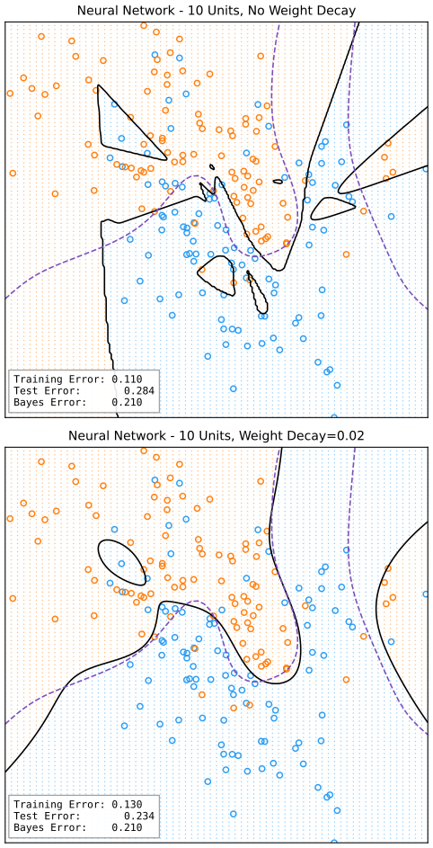
fig_11_4. Reproduces Hastie, Tibshirani and Friedman (2009), Figure 11.4. Download: PDF · SVG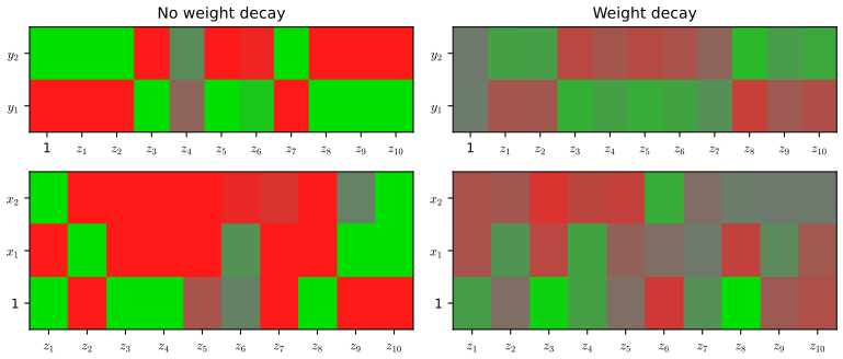
fig_11_5. Reproduces Hastie, Tibshirani and Friedman (2009), Figure 11.5. Download: PDF · SVG11.5.3 Scaling of the Inputs
pp. 398–400 The scale of the inputs sets the effective scale of the bottom-layer weights, so it can change the final fit a great deal. The advice is to standardise every input to mean zero and standard deviation one at the outset: this treats the inputs equally in the regularisation and makes a meaningful range for the random starting weights possible; with standardised inputs the weights are typically drawn uniformly on \([-0.7,0.7]\).
See also (companion course): Foundations of Deep Learning, Section 7.4.1 and Filling the gap 7.7 (what normalising the inputs does to the Hessian).
Filling the gap 11.7: what the scale of an input changes, and why \([-0.7,0.7]\) p. 400
Derivation
The model does not care; the penalty and the start do. If input \(j\) is multiplied by \(c\ne0\), dividing every \(\alpha_{mj}\) by \(c\) gives exactly the same network, so the set of fitted functions is unchanged. But the penalty (11.16) charges \(\alpha_{mj}^2\), which becomes \(\alpha_{mj}^2/c^2\): measuring an input in larger units (\(c>1\)) makes its weights cheaper, measuring it in smaller units makes them dearer. Weight decay is therefore not scale invariant, exactly like ridge regression, and the inputs must be put on a common scale before the penalty means anything. The same rescaling changes the distribution of the starting values relative to the fitted ones.
The starting range. With independent standardised inputs and weights \(U[-a,a]\) independent of the inputs, the activation \(a_m=\alpha_{0m}+\sum_{j=1}^p\alpha_{mj}x_j\) has mean 0 and variance \((p+1)a^2/3\) (each term has variance \(\E\alpha^2\E x_j^2=a^2/3\)). With \(a=0.7\) the standard deviation is \(0.40\sqrt{p+1}\): \(0.70\) for \(p=2\) and \(1.3\) for \(p=10\). By Result 11.7 the nonlinear part of a unit is then at most \(|a_m|^3/48\), e.g. \(0.007\) at \(|a_m|=0.7\): the network starts almost linear, as Section 11.5.1 wants, and the units are not saturated, so the gradients are not tiny. For many inputs the same rule saturates the units: with \(p=256\) (the ZIP code images), \(0.40\sqrt{257}=6.5\). That is why the starting range should shrink with the number of inputs to a unit, e.g. uniform on \(\pm2.4/F\) for fan-in \(F\) as in Le Cun's networks of Section 11.7 (activation standard deviation at most \(2.4/\sqrt{3F}\approx0.09\) for \(F=257\)), and why modern initialisations scale with \(1/\sqrt F\) (Foundations of Deep Learning, Result 7.5). ∎
11.5.4 Number of Hidden Units and Layers
p. 400 It is generally better to have too many hidden units than too few: too few cannot capture the nonlinearities, while the weights of extra units can be shrunk toward zero by regularisation. Typical numbers are 5 to 100, growing with the number of inputs and of training cases; the common practice is to use a reasonably large number and train with regularisation. Choosing the number by cross-validation is possible but seems unnecessary when cross-validation already chooses \(\lambda\). The number of hidden layers is a matter of background knowledge and experiment; each layer extracts features of the one below, and several layers build a hierarchy of features at different resolutions (Section 11.7).
11.5.5 Multiple Minima
pp. 400–401 \(R(\theta)\) is nonconvex with many local minima, so the solution depends on the starting weights. At the least one should try several random starts and keep the solution with the lowest penalised error; probably better is to average the predictions of the networks (Ripley, 1996), rather than their weights, because the model is nonlinear in the weights. Bagging (Section 8.7) averages networks trained on bootstrap samples instead.
See also (companion courses): Foundations of Deep Learning, Section 9.6 (committees, Result 9.11); Bayesian and Probabilistic Machine Learning, Section 14.2.
Result 11.9 (average predictions, not weights) p. 401
(a) For predictions \(\hat f_1(x),\dots,\hat f_L(x)\) with average \(\bar f(x)\) and any response \(y\),
\[ (y-\bar f(x))^2=\frac1L\sum_{l=1}^L(y-\hat f_l(x))^2-\frac1L\sum_{l=1}^L(\hat f_l(x)-\bar f(x))^2. \]So the averaged prediction's squared error never exceeds the average of the members' squared errors, at every \(x\) and hence for every test set, and the gain is the spread of the members (the "ambiguity").
(b) Averaging weights has no such guarantee. If \(\theta\) is a fitted network and \(\pi\theta\) the same network with two hidden units swapped, both predict identically, yet \((\theta+\pi\theta)/2\) is a different network; if the two units are sign-flipped copies of each other (Filling the gap 11.2), averaging can cancel them entirely.
Proof
(a) Write \(y-\hat f_l=(y-\bar f)-(\hat f_l-\bar f)\) and square: \[ \frac1L\sum_l(y-\hat f_l)^2=(y-\bar f)^2-\frac2L(y-\bar f)\sum_l(\hat f_l-\bar f)+\frac1L\sum_l(\hat f_l-\bar f)^2 \], and the middle sum is zero. (b) Take \(M=2\), \(\theta\) with units \((\alpha_{01},\alpha_1,\beta_1)\) and \((\alpha_{02},\alpha_2,\beta_2)\). The swapped network has the same function. The average has both units equal to \(((\alpha_{01}+\alpha_{02})/2,(\alpha_1+\alpha_2)/2)\) with output weights \((\beta_1+\beta_2)/2\): a one-unit network in disguise. If moreover \((\alpha_{02},\alpha_2,\beta_2)=(-\alpha_{01},-\alpha_1,-\beta_1)\), the averaged units have zero weights and output weight zero: a constant. ∎
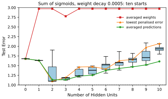
fig_11_s1.How strongly does the solution depend on the start? Even a change in the data far below any measurement precision can move a fit to a different minimum: in these experiments, multiplying all 100 responses by \(1+10^{-15}\) changed the relative test error of one of seven networks checked with weight decay 0.0005 by 0.22 (it ended in another minimum), and with no decay three of the seven moved by more than 0.1 (up to 0.9). Only strongly penalised fits (\(\lambda=0.1\)) were stable to many digits. Weight decay therefore also makes the fitting problem better posed.
11.6 Example: Simulated Data
pp. 401–404 Two additive-error models \(Y=f(X)+\varepsilon\) with standard Gaussian inputs:
\[ \text{Sum of sigmoids: }Y=\sigma(a_1^\T X)+\sigma(a_2^\T X)+\varepsilon_1;\qquad\text{Radial: }Y=\prod_{m=1}^{10}\phi(X_m)+\varepsilon_2, \]with \(p=2\), \(a_1=(3,3)\), \(a_2=(3,-3)\) in the first, \(p=10\) and \(\phi(t)=(2\pi)^{-1/2}e^{-t^2/2}\) in the second, and Gaussian errors whose variance makes the signal-to-noise ratio
\[ \frac{\Var(\E(Y\given X))}{\Var(Y-\E(Y\given X))}=\frac{\Var(f(X))}{\Var(\varepsilon)} \tag{11.18} \]equal to 4. The training sample has 100 cases and the test sample 10,000. Test errors are reported relative to the Bayes error \(\Var(\varepsilon)\), the smallest possible expected squared error.
Result 11.10 (the two signals, exactly) pp. 401–402
(a) For the sum of sigmoids, \(a_1^\T X\) and \(a_2^\T X\) are independent \(N(0,18)\), and
\[ \Var f(X)=2\Big(\E\,\sigma(3\sqrt2Z)^2-\tfrac14\Big)=0.32652,\qquad Z\sim N(0,1), \]so the noise variance is \(0.08163\) (standard deviation 0.286).
(b) For the radial function, \(\E f(X)=(2\sqrt\pi)^{-10}=3.19\times10^{-6}\) and
\[ \Var f(X)=\Big(\frac1{2\pi\sqrt3}\Big)^{10}-\Big(\frac1{2\sqrt\pi}\Big)^{20}=3.27\times10^{-11}. \](c) In both models the constant predictor \(\E f(X)\) has expected test error \(\Var f+\Var\varepsilon\), i.e. relative error \(1+\text{SNR}=5\); the sample mean of the training responses adds a factor \(1+1/N\). For the radial model \(\E[f(X)X_j]=0\), so the best linear predictor is the constant too.
Proof
(a) \(a_1^\T X\) and \(a_2^\T X\) are jointly Gaussian with variances \(9+9=18\) and covariance \(9-9=0\), hence independent, so \(\Var f\) is the sum of the two variances, each \(\Var\sigma(3\sqrt2Z)\). Since \(\sigma(-v)=1-\sigma(v)\) and \(Z\) is symmetric, \(\E\sigma(cZ)=\tfrac12\); so \(\Var\sigma(cZ)=\E\sigma(cZ)^2-\tfrac14\), a one-dimensional integral (computed by quadrature: \(0.16326\)).
(b) The coordinates are independent, so \(\E f=(\E\phi(X_1))^{10}\) and \(\E f^2=(\E\phi(X_1)^2)^{10}\). Now \(\E\phi(X_1)=\int\phi^2=\frac1{2\pi}\int e^{-t^2}\d t=\frac{\sqrt\pi}{2\pi}=\frac1{2\sqrt\pi}\) and \[ \E\phi(X_1)^2=\int\phi^3=(2\pi)^{-3/2}\int e^{-3t^2/2}\d t=(2\pi)^{-3/2}\sqrt{2\pi/3}=\frac1{2\pi\sqrt3} \]. Subtract the squared mean.
(c) For any constant \(c\), \(\E(Y-c)^2=\Var f+\Var\varepsilon+(\E f-c)^2\), minimised at \(c=\E f\); divide by \(\Var\varepsilon=\Var f/4\). The training mean \(\bar y\) is independent of a new case and has variance \((\Var f+\Var\varepsilon)/N\). Finally \(f\) is even in each \(X_j\) and \(X_j\) is symmetric, so \(\E[f(X)X_j]=0\): the population least-squares coefficients of the inputs are zero. ∎
Note on the book: the scale of the radial example
By Result 11.10(b), the radial signal has standard deviation \(5.7\times10^{-6}\) and the noise \(2.9\times10^{-6}\). On that scale the residual sum of squares of 100 points is of order \(10^{-9}\), while the penalty \(0.0005\sum\theta^2\) of any network with weights of order one is of order \(10^{-3}\): the stated weight decay would shrink every network to (nearly) zero output, and the relative error would be about \(1+(3.19^2+5.72^2)/2.86^2\approx6.2\) for every number of hidden units, not the rising curve of Figure 11.6. The book does not say how the response was scaled. Here the radial function is divided by its standard deviation (so \(\Var f=1\) and \(\Var\varepsilon=1/4\)), which leaves every relative error unchanged and makes the decay 0.0005 mean the same as for the sum of sigmoids (whose signal variance is 0.33). Under this reading the reproduction matches the book's picture.
The networks are fitted with weight decay and \(0,1,\dots,10\) hidden units (zero units means linear least squares), each from ten random starts, and the test error is computed for each. Only one training set is generated; the book says the results are typical of an "average" training set. The network is perfectly suited to the sum of sigmoids, and two units come close to the Bayes rate; with more units overfitting creeps in, and some starts do worse than the linear model. The radial function, spherically symmetric with no preferred direction, is the hardest case for a network: it does worse than the constant fit.
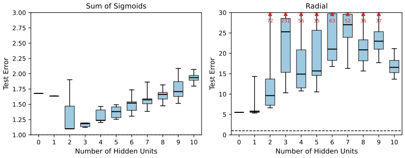
fig_11_6. Reproduces Hastie, Tibshirani and Friedman (2009), Figure 11.6. Download: PDF · SVGThe linear model's 5.53 against the constant's 5 is the price of estimating 11 useless coefficients from 100 points: about \(5\times11/100=0.55\) in relative error. In Figure 11.6 the decay of 0.0005 is mild. Figure 11.7 repeats the sum of sigmoids with no decay and with \(\lambda=0.1\); Figure 11.8 varies \(\lambda\) for ten units.
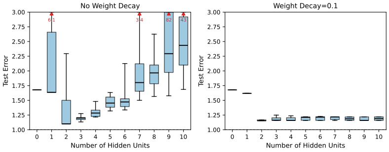
fig_11_7. Reproduces Hastie, Tibshirani and Friedman (2009), Figure 11.7. Download: PDF · SVG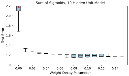
fig_11_8. Reproduces Hastie, Tibshirani and Friedman (2009), Figure 11.8. Download: PDF · SVGThere are two tuning parameters, \(\lambda\) and \(M\). One strategy fixes one of them at its least constrained value (\(\lambda=0\), or the largest \(M\)) and cross-validates the other. Comparing Figure 11.7 (left) with Figure 11.8 shows that the test error is much less sensitive to \(\lambda\) near its optimum than to \(M\) without decay, so cross-validating \(\lambda\) at a generous \(M\) is preferable.
11.7 Example: ZIP Code Data
pp. 404–408 Handwritten digits scanned from envelopes, deslanted and size-normalised to 16×16 grey-level images (Figure 11.9); the 256 pixel values are the inputs. A generic network is not ideal for images because pixels lack invariances (a small shift or rotation changes every input), and early networks made about 4.5% errors. The example follows Le Cun's (1989) handcrafted networks, which led to the convolutional networks of Le Cun et al. (1998). To make the effects visible the sample is small: 320 training and 160 test digits, built from scanned digits plus copies with random horizontal shifts.
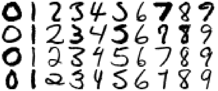
fig_11_9. Reproduces Hastie, Tibshirani and Friedman (2009), Figure 11.9 (with digits drawn at random from zip.train). Download: PDF · SVGFive networks were fitted (Figure 11.10 of the book is their diagram; the demonstration draws them live):
- Net-1: no hidden layer: 256 inputs, 10 outputs; nearly multinomial logistic regression (Exercise 11.4).
- Net-2: one hidden layer of 12 fully connected units.
- Net-3: two locally connected hidden layers. Layer 1 is an 8×8 array in which each unit sees a 3×3 patch of the image; units one apart in the array have patches two pixels apart (overlapping by one row or column). Layer 2 is a 4×4 array, each unit seeing a 5×5 patch of layer 1, again two apart. All other connections are zero.
- Net-4: as Net-3, but layer 1 consists of two 8×8 feature maps; all units of a map share the same nine weights (each has its own bias). Layer 2 is locally connected without sharing.
- Net-5: layer 1 as in Net-4; layer 2 has four 4×4 feature maps, each unit connected to 5×5 patches of both layer-1 maps, with weights shared within each map.
All have sigmoidal output units and are fitted by back-propagation on the squared error; the output \(\hat f_k(x)\) estimates the probability of class \(k\). Every network has more weights than training cases, and all reach 0% training error. Local connectivity makes each unit a local feature extractor and cuts the number of weights; sharing forces the same local feature to be computed everywhere, which is what makes these networks convolutional. The book's Table 11.1 lists links (connections) and weights (free parameters):
Result 11.11 (links and weights of the five networks; Table 11.1) p. 407
| network | architecture | links | weights | % correct (book) |
|---|---|---|---|---|
| Net-1 | single layer | 2570 | 2570 | 80.0 |
| Net-2 | two layers, 12 hidden units | 3214 | 3214 | 87.0 |
| Net-3 | locally connected | 1226 | 1226 | 88.5 |
| Net-4 | constrained network 1 | 2266 | 1132 | 94.0 |
| Net-5 | constrained network 2 | 5194 | 1060 | 98.4 |
All five counts follow from the architectures above, counting each bias as one link and one weight, with every unit (shared or not) having its own bias.
Proof (the counts)
A fully connected layer from \(n\) to \(m\) units has \(m(n+1)\) links and weights. A layer of \(u\) units each seeing \(q\) inputs has \(u(q+1)\) links; without sharing that is also its number of weights, with one shared kernel per map it has (kernel size) × (maps) + \(u\) weights.
- Net-1: \(10\times257=2570\).
- Net-2: \(12\times257+10\times13=3084+130=3214\).
- Net-3: layer 1, \(64\times(9+1)=640\); layer 2, \(16\times(25+1)=416\); output, \(10\times17=170\); total 1226 links = weights.
- Net-4: layer 1 has \(2\times64=128\) units, \(128\times10=1280\) links but only \(2\times9+128=146\) weights; layer 2, \(16\) units each seeing \(2\times25\) inputs, \(16\times51=816\) links and weights; output 170. Links \(1280+816+170=2266\); weights \(146+816+170=1132\).
- Net-5: layer 1 as Net-4 (1280 links, 146 weights); layer 2, \(4\times16=64\) units each seeing \(2\times25\) inputs: \(64\times51=3264\) links, \(4\times50+64=264\) weights; output \(10\times65=650\). Links \(1280+3264+650=5194\); weights \(146+264+650=1060\). ∎
The book's "errors of only 1.6%, compared to 13% for the vanilla network Net-2" is the table's 98.4% and 87.0%. The gradient for a shared weight needs one more line:
Result 11.12 (the gradient of a shared weight) p. 407
If one parameter \(w\) is the value of the links \(c\in\mathcal C(w)\), then \(\partial R/\partial w=\sum_{c\in\mathcal C(w)}\partial R/\partial w_c\), where \(\partial R/\partial w_c\) is the derivative computed by back-propagation as if link \(c\) had its own weight.
Proof
Let \(\tilde R(\{w_c\})\) be the error as a function of separate link weights; the shared network's error is \(R(w)=\tilde R(w,w,\dots,w)\). By the chain rule for the map \(w\mapsto(w,\dots,w)\), \(R'(w)=\sum_c\partial\tilde R/\partial w_c\) evaluated at equal weights. For a convolutional feature map this sum over positions is a cross-correlation of the layer's errors with its input, Foundations of Deep Learning, Result 10.4; see also Filling the gap 9.9 there. ∎
See also (companion courses): Foundations of Deep Learning, Filling the gap 10.4 (a convolutional layer is a sparse, weight-shared fully connected layer) and Result 10.3 (receptive fields); Bayesian and Probabilistic Machine Learning, Result 5.16.
The reproduction. Le Cun's 320/160 digit set is not distributed with the book, so Figure 11.11 is redone at CPU scale in the same spirit: 160 digits of zip.train (16 per class), each used twice with independent random horizontal shifts of up to two pixels (320 training images), and all 2007 digits of zip.test, each shifted once. Each network has tanh hidden units and logistic outputs, starting weights uniform on \(\pm2.4/F\) (\(F\) the fan-in), and is trained by on-line back-propagation of the squared error for 30 epochs, five times from different starts.
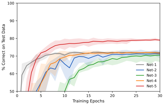
fig_11_11. Reproduces Hastie, Tibshirani and Friedman (2009), Figure 11.11, at CPU scale with different data. Download: PDF · SVGWhat carries over and what does not. The parameter counts are exact. The network with two levels of weight sharing is clearly the best (by 7 points, far beyond the run-to-run spread of about 1 point), with the fewest weights. The others end close together, and none of the book's 7-point gaps between Net-1, Net-2 and Net-3 appears: on the much harder public test set (different writers from the training set) and with only 160 distinct training digits, every network is limited by the data, and the linear Net-1 learns fastest because its error surface is convex. Net-4 does reach its plateau faster than Net-3, as sharing should make it. The book's own point stands: the gains come from building knowledge of the problem (locality, shift invariance) into the architecture, not from more weights; the design of Net-5 "was the result of many person years of experimentation".
The later history: tangent distance (Simard et al., 1993; Section 13.3.3) beat these networks by building in affine invariances explicitly, and digit recognition became a test bed for every new method. On a database of 60,000 training and 10,000 test digits, Le Cun et al. (1998) report 1.1% error for tangent distance with 1-nearest neighbour, 0.8% for a degree-9 polynomial SVM, 0.8% for LeNet-5 and 0.7% for boosted LeNet-4. They quote a standard error of 0.1%, so error rates within 0.1–0.2% of each other are statistically equivalent; and since the test set was used, implicitly, to tune the methods, the real uncertainty is larger.
Filling the gap 11.8: the standard error of an error rate, and of a difference p. 408
Derivation
If a classifier errs independently on each of \(N\) test cases with probability \(p\), the observed rate \(\hat p\) has standard error \(\sqrt{p(1-p)/N}\). With \(N=10{,}000\) and \(p\approx0.01\): \(\sqrt{0.01\times0.99/10^4}=0.00099\approx0.1\%\).
For a difference of two rates the answer depends on whether the test sets are the same. On independent test sets the variances add: \(\sqrt2\times0.1\%\approx0.14\%\), so a difference of 0.2% is about 1.4 standard errors and 0.1% about 0.7, which is why differences in the 0.1–0.2% range are not significant. On the same test set, write \(n_{10}\) and \(n_{01}\) for the cases that exactly one of the two classifiers gets wrong; then \(\hat p_A-\hat p_B=(n_{10}-n_{01})/N\) and, conditionally on the discordant total \(n_{10}+n_{01}\), \(n_{10}\) is binomial with probability \(\tfrac12\) under equal accuracy (McNemar's test), giving standard error \(\sqrt{n_{10}+n_{01}}/N\). Two good classifiers share most of their errors, so the paired standard error is usually smaller than \(0.14\%\); the book's error bars in Figure 11.12 use the unpaired form. ∎
11.8 Discussion
pp. 408–409 Projection pursuit and networks both model nonlinear functions of linear combinations of the inputs; this is a powerful general approach that competes well with the best learning methods. It works best when the signal-to-noise ratio is high and prediction, not interpretation, is the goal. It is much less suited to describing how the data were generated or what role each input plays, because each input enters the model in many places, nonlinearly. Plotting the weights into each hidden unit (Hinton, 1989) is limited by non-identifiability (Filling the gap 11.2): beyond the exact symmetries, there are often quite different weight vectors \(\alpha_m\) spanning roughly the same linear space and giving nearly the same predictions; a principal component analysis of the fitted weights has been suggested as a way to find an interpretable version. This has limited the use of networks where interpretation matters, such as medicine. On the other hand, networks are smooth functions of real parameters (unlike CART and MARS), which makes Bayesian inference for them feasible.
11.9 Bayesian Neural Nets and the NIPS 2003 Challenge
pp. 409–414 A classification competition held for a workshop of the 2003 Neural Information Processing Systems conference gave participants five labelled two-class training sets from different domains (Table 11.2), with the features of a validation set. For 12 weeks they could submit validation-set predictions and see their scores; they then submitted test-set predictions; finally the validation labels were released and they had one week to refit on training plus validation data and submit final predictions. Of 75 groups, 20 and 16 submitted on the validation and test sets. The challenge stressed feature selection: artificial probes, noise features distributed like the real ones but independent of the class, were added to every data set, so each method had to find and downweight them. Entries were scored by test accuracy, area under the ROC curve and a combined head-to-head score (Guyon et al., 2006).
| data set | domain | features | \(p\) | % probes | \(N_{\rm tr}\) | \(N_{\rm val}\) | \(N_{\rm te}\) |
|---|---|---|---|---|---|---|---|
| Arcene | mass spectrometry | dense | 10,000 | 30 | 100 | 100 | 700 |
| Dexter | text classification | sparse | 20,000 | 50 | 300 | 300 | 2000 |
| Dorothea | drug discovery | sparse binary | 100,000 | 50 | 800 | 350 | 800 |
| Gisette | digit recognition | dense | 5000 | 30 | 6000 | 1000 | 6500 |
| Madelon | artificial | dense | 500 | 96 | 2000 | 600 | 1800 |
The five data sets of the challenge (the facts of the book's Table 11.2).
The clear overall winners were Neal and Zhang (2006): first on three data sets, fifth and seventh on the other two. They used feature-selection preprocessing followed by Bayesian neural networks, Dirichlet diffusion trees and combinations of these. The book focuses on the Bayesian networks and asks which ingredients mattered, rerunning their programs against boosted and bagged networks, boosted trees and random forests.
11.9.1 Bayes, Boosting and Bagging
pp. 410–412 Given training data \(\bX_{\rm tr},\by_{\rm tr}\) and a sampling model \(\Pr(Y\given X,\theta)\) (for Neal and Zhang, a network with two hidden layers whose output is the class probability) with prior \(\Pr(\theta)\), the posterior is
\[ \Pr(\theta\given\bX_{\rm tr},\by_{\rm tr})=\frac{\Pr(\theta)\Pr(\by_{\rm tr}\given\bX_{\rm tr},\theta)}{\int\Pr(\theta)\Pr(\by_{\rm tr}\given\bX_{\rm tr},\theta)\,\d\theta} \tag{11.19} \]and the predictive distribution of a new label is
\[ \Pr(Y_{\rm new}\given X_{\rm new},\bX_{\rm tr},\by_{\rm tr})=\int\Pr(Y_{\rm new}\given X_{\rm new},\theta)\Pr(\theta\given\bX_{\rm tr},\by_{\rm tr})\,\d\theta \tag{11.20} \](compare Section 8.3). The integral is intractable; a few hundred draws \(\theta_\ell\) from the posterior (11.19), obtained by Markov chain Monte Carlo, give the estimate \(\frac1L\sum_\ell\Pr(Y_{\rm new}\given X_{\rm new},\theta_\ell)\). Neal and Zhang used diffuse Gaussian priors and hybrid (Hamiltonian) Monte Carlo, which adds an auxiliary momentum vector and follows Hamiltonian dynamics with the negative log posterior as potential energy, so that successive draws move far through the parameter space instead of random-walking, are less correlated, and converge faster.
See also (companion courses): Bayesian and Probabilistic Machine Learning, Section 5.7 (Bayesian networks by the Laplace approximation) and Section 11.5.2 (hybrid Monte Carlo, with proofs); Section 8.6 of this course (MCMC).
Result 11.13 (hybrid Monte Carlo samples the posterior)
Let \(U(\theta)=-\log[\Pr(\theta)\Pr(\by_{\rm tr}\given\bX_{\rm tr},\theta)]\). From \(\theta\), draw momenta \(\rho\sim N(0,\mathbf I)\), run \(L\) leapfrog steps with step sizes \(\epsilon_i\) (one per coordinate, fixed during the trajectory),
\[ \rho\leftarrow\rho-\tfrac{\epsilon}2\odot\nabla U(\theta),\quad\theta\leftarrow\theta+\epsilon\odot\rho,\quad\rho\leftarrow\rho-\tfrac\epsilon2\odot\nabla U(\theta), \]and accept the end point \((\theta^*,\rho^*)\) with probability \(\min\{1,\exp(H(\theta,\rho)-H(\theta^*,\rho^*))\}\), \(H=U+\tfrac12\|\rho\|^2\). This Markov chain leaves the posterior (11.19) invariant, whatever \(\epsilon\) and \(L\).
Proof sketch
Target the joint density \(\propto e^{-H(\theta,\rho)}\), whose \(\theta\)-marginal is the posterior. Redrawing \(\rho\) is a Gibbs step for it. Each half-step and full step of the leapfrog is a shear (it changes one block of variables by a function of the other block), so it has Jacobian determinant 1, and the composition is volume preserving; the leapfrog map followed by a reversal of \(\rho\) is its own inverse. A deterministic, volume-preserving involution followed by a Metropolis test with ratio \(e^{-H^*}/e^{-H}\) satisfies detailed balance with respect to \(e^{-H}\). Per-coordinate step sizes are the same as a diagonal mass matrix. The full proof is in Bayesian and Probabilistic Machine Learning, Section 11.5.2. If the step sizes depend on the current hyperparameters (as here: \(\epsilon_i\) proportional to the prior standard deviation of weight \(i\)), the argument holds conditionally on them, and alternating with a Gibbs step for the hyperparameters leaves the joint posterior invariant. Adapting \(\epsilon\) from the acceptance rate is allowed during burn-in only. ∎
Neal and Zhang also tried two kinds of preprocessing: (1) univariate screening by \(t\)-tests, and (2) automatic relevance determination (ARD), in which the weights from input \(j\) to all first-layer units share one prior variance \(\sigma_j^2\) (prior mean zero); the posterior of each \(\sigma_j^2\) is computed, and features whose \(\sigma_j\) concentrates on small values are dropped.
Filling the gap 11.9: how the posterior of an ARD variance is computed p. 411
Derivation
Parametrise by the precision \(\tau_j=1/\sigma_j^2\) with a Gamma prior of shape \(a\) and rate \(b\), \(p(\tau_j)\propto\tau_j^{a-1}e^{-b\tau_j}\). Given \(\tau_j\), the \(H_1\) weights \(w_{j1},\dots,w_{jH_1}\) out of input \(j\) are independent \(N(0,1/\tau_j)\), with joint density \(\propto\tau_j^{H_1/2}\exp(-\tau_j\sum_mw_{jm}^2/2)\). The likelihood depends on \(\tau_j\) only through these weights, so
\[ p(\tau_j\given\theta,\text{data})\propto\tau_j^{a+H_1/2-1}\exp\Big\{-\Big(b+\tfrac12\sum_{m=1}^{H_1}w_{jm}^2\Big)\tau_j\Big\}, \]a Gamma distribution with shape \(a+H_1/2\) and rate \(b+\tfrac12\sum_mw_{jm}^2\). Sampling it given the current weights is a Gibbs step; the same conjugate update serves the precisions of the other groups of weights (biases, second layer, output). If input \(j\) is irrelevant, the likelihood does not push its weights away from zero, \(\sum_mw_{jm}^2\) stays small and the draws of \(\tau_j\) are large: \(\sigma_j\) concentrates near zero and the input is effectively switched off. Relevance is read from the posterior of \(\sigma_j\), e.g. its median over the draws. ∎
Three ingredients might explain the success: (a) the feature selection and preprocessing, (b) the network model, (c) Bayesian inference by MCMC. According to Neal and Zhang, (a) was done only to save computation (MCMC is slow with many features); overfitting needs no feature selection because the posterior average (11.20) takes care of it. The book's view is that the power of modern Bayesian methods lies less in formal inference (few would believe the priors of a large network are correct) than in the fact that MCMC samples the relevant parts of model space efficiently and averages the predictions of the high-probability models.
Bagging and boosting have a similar flavour. The Bayesian approach fixes the data and perturbs the parameters according to the current posterior; bagging perturbs the data i.i.d. (bootstrap samples), refits, and averages; boosting fits a model that is additive in base learners, each fitted to non-i.i.d. (reweighted) data. All three have the form
\[ \hat f(x_{\rm new})=\sum_{\ell=1}^Lw_\ell\,\E(Y_{\rm new}\given x_{\rm new},\hat\theta_\ell), \tag{11.21} \]with \(\hat\theta_\ell\) a large collection of parameter values: for the Bayesian model, posterior draws with \(w_\ell=1/L\) (an estimate of the posterior mean (11.20)); for bagging, fits to bootstrap samples with \(w_\ell=1/L\); for boosting, a sequence chosen deterministically to keep improving the fit, with \(w_\ell=1\) (the shrinkage factor, if any, absorbed into the terms).
Note on the book: two slips in Section 11.9.1
(i) Page 410 says MCMC methods are used "to sample from the posterior distribution \(\Pr(Y_{\rm new}\given X_{\rm new},\bX_{\rm tr},\by_{\rm tr})\)". The chain samples the parameters from \(\Pr(\theta\given\bX_{\rm tr},\by_{\rm tr})\), (11.19); the predictive probability (11.20) is then estimated by averaging \(\Pr(Y_{\rm new}\given X_{\rm new},\theta_\ell)\) over the draws, as the next sentence of the book says. (ii) Page 412 says that for the Bayesian model "the average estimates the posterior mean (11.21)"; the posterior mean is (11.20), and (11.21) is the general weighted average that covers all three methods.
11.9.2 Performance Comparisons
pp. 412–414 The book compares, on the five data sets: Bayesian networks (Neal and Zhang's results; two hidden layers of 20 and 8 units); boosted trees (R package gbm, tree depth 2–9, shrinkage 0.001–0.1, 80% subsampling per iteration); boosted networks (single hidden layer of two or four units, R package nnet); random forests (R package randomForest, default settings); and bagged networks with the Bayesian architecture. The analysis, by Nicholas Johnson (2008), used both the univariate-screened features and the ARD-reduced features. Its Figure 11.12 shows the test errors (not reproduced: the challenge data and the entries' programs are not part of the book's material), with error bars of one standard error of a difference of two rates; its Table 11.3 gives average ranks and times:
| method | avg. rank, screened | time, screened (min) | avg. rank, ARD | time, ARD (min) |
|---|---|---|---|---|
| Bayesian neural networks | 1.5 | 384 (138) | 1.6 | 600 (186) |
| boosted trees | 3.4 | 3.03 (2.5) | 4.0 | 34.1 (32.4) |
| boosted neural networks | 3.8 | 9.4 (8.6) | 2.2 | 35.6 (33.5) |
| random forests | 2.7 | 1.9 (1.7) | 3.2 | 11.2 (9.3) |
| bagged neural networks | 3.6 | 3.5 (1.1) | 4.0 | 6.4 (4.4) |
The book's Table 11.3: average rank of the test error over the five problems (low is good) and mean computing time with its standard error.
The Bayesian networks win again, although on some data sets the differences are within the standard error. Random forests are the best competitor with the screened features, boosted networks with the reduced features (nearly matching the Bayesian networks). That boosted networks beat boosted trees suggests that the network model suits these problems (linear combinations of features predict better than individual features), but the strong showing of random forests does not fit this explanation and surprised the authors. Since the ARD features come from the Bayesian networks, only the screened-feature methods are self-contained; better internal feature selection might help boosted networks. The non-Bayesian methods are far faster. The book concludes that the Bayesian networks did well because (a) the network model suits these five problems and (b) MCMC explores the important part of the parameter space and averages the resulting models by their quality; Bayesian methods work well for smoothly parametrised models like networks, and it is not yet clear that they do for non-smooth ones like trees.
A CPU-scale rerun. The comparison can be repeated in a few minutes on one problem built like Madelon (the artificial data set of the challenge): 100 features, of which 5 informative (classes formed by Gaussian clusters at vertices of a hypercube), 10 linear combinations of them and 85 probes; 500 training and 2000 test cases. The five methods are reimplemented as closely as is practical: a Bayesian network with hidden layers of 20 and 8 tanh units, ARD priors and Gamma hyperpriors, sampled by hybrid Monte Carlo (Result 11.13) with Gibbs steps for the precisions (Filling the gap 11.9), 1000 iterations of 40 leapfrog steps, the second half kept; gradient-boosted trees (depth 4, shrinkage 0.05, 80% subsampling, 400 trees); gradient boosting of the binomial deviance with four-unit networks as base learners (200 rounds, shrinkage 0.1); random forests (500 trees, default settings); 25 bagged networks with the Bayesian architecture fitted by penalised maximum likelihood. "Screened" keeps the 20 features with the largest two-sample \(|t|\); "ARD reduced" keeps the features whose posterior median \(\sigma_j\) in an ARD network fitted to all 100 features exceeds half the largest.
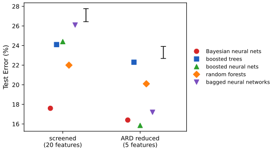
fig_11_s3.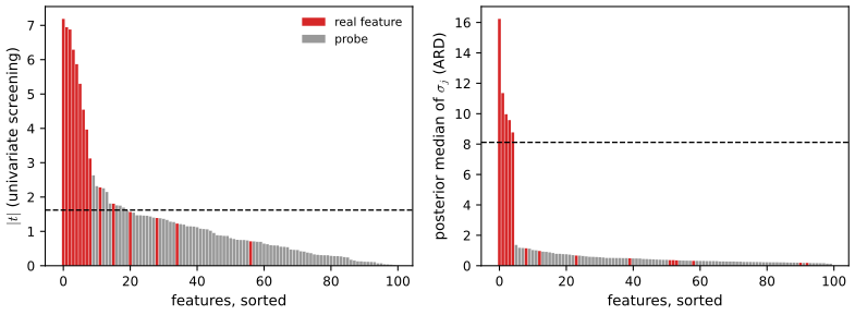
fig_11_s4.The book\'s pattern survives the change of scale. With the screened features the Bayesian network is best (17.6%) and random forests are the best competitor (22.0%); the Bayesian network\'s lead over every other method is 3 to 6 standard errors of a difference. With the ARD features the boosted networks come first (15.9%), within half a standard error of the Bayesian network (16.4%), as in the book\'s Table 11.3 where boosted networks rank 2.2 against 1.6. Average ranks over the two feature sets: Bayesian networks 1.5, random forests 3, boosted networks 2.5, bagged networks 4, boosted trees 4. The Bayesian network took 20 and 16 seconds, plus 32 seconds for the ARD run on all 100 features, against 1 to 15 seconds for the others: the same ordering of costs as in the book, at a thousandth of the scale. The ARD features help every method, the networks most (bagged networks from 26.1% to 17.2%), which supports the book\'s remark that better internal feature selection would help the non-Bayesian networks; and the probes are what defeats univariate screening, which keeps 9 probes among its 20 features.
11.10 Computational Considerations
p. 414 With \(N\) observations, \(p\) inputs, \(M\) hidden units and \(L\) training epochs, fitting a network takes \(O(NpML)\) operations. Software for networks is plentiful and of uneven quality, and the fit is sensitive to input scaling and starting values, so it should be chosen and checked with care.
Filling the gap 11.10: where \(O(NpML)\) comes from p. 414
Derivation
For one case, the forward pass computes \(M\) activations \(\alpha_{0m}+\alpha_m^\T x\) (\(M(p+1)\) multiply-adds), \(M\) sigmoids, and \(K\) outputs (\(K(M+1)\) multiply-adds). The backward pass computes \(K\) output errors, the \(M\) hidden errors (11.15) (\(KM\)) and the gradients (11.14) (\(K(M+1)+M(p+1)\)). So one case costs \(O(M(p+K))\), which is \(O(pM)\) when \(K\le p\), as is usual; an epoch over \(N\) cases costs \(O(NpM)\) and \(L\) epochs \(O(NpML)\). Back-propagation is what makes this linear in the number of weights \(W=M(p+1)+K(M+1)\): differencing the error numerically would cost \(O(W)\) forward passes per gradient, i.e. \(O(NW^2)\) (Foundations of Deep Learning, Result 8.2). A quasi-Newton iteration (Filling the gap 11.4) adds \(O(W^2)\) per iteration for the matrix update, negligible when \(N\) is much larger than \(W\). ∎
Bibliographic Notes
p. 415 Projection pursuit was proposed by Friedman and Tukey (1974) and specialised to regression by Friedman and Stuetzle (1981); Huber (1985) gives a scholarly overview and Roosen and Hastie (1994) a formulation with smoothing splines. Neural networks go back to McCulloch and Pitts (1943), Widrow and Hoff (1960) and Rosenblatt (1962), with Hebb (1949) a strong influence on learning rules; their resurgence in the mid-1980s followed the back-propagation algorithm of Werbos (1974), Parker (1985) and Rumelhart et al. (1986). For readers of the book, Hertz et al. (1991), Bishop (1995) and Ripley (1996) are the most informative texts; Bayesian learning for networks is Neal (1996); the ZIP code example is from Le Cun (1989), see also Le Cun et al. (1990, 1998). Approximation properties (Barron, 1993; Girosi et al., 1995; Jones, 1992) are not discussed in the book; Results 11.2 and 11.4 above give the basic density statement.
Exercises
All 7 exercises of Chapter 11 (Hastie, Tibshirani and Friedman, 2009, pp. 415–416), restated in my own words, with complete solutions (hidden). The computations are in the chapter code.
Exercise 11.1. Make the correspondence between projection pursuit regression (11.1) and the network (11.5) exact: show that a single-hidden-layer regression network is a PPR model with \(g_m(\omega_m^\T x)=\beta_m\sigma(\alpha_{0m}+s_m\omega_m^\T x)\), \(\omega_m\) a unit vector. Do the same for a classification network.
Solution
Regression. Take \(K=1\) and the identity output. For each unit with \(\alpha_m\ne0\) set \(s_m=\|\alpha_m\|\), \(\omega_m=\alpha_m/s_m\); then \(\alpha_m^\T x=s_m\omega_m^\T x\) and
\[ f(x)=\beta_0+\sum_{m=1}^M\beta_m\sigma(\alpha_{0m}+s_m\,\omega_m^\T x)=\sum_{m=1}^Mg_m(\omega_m^\T x),\qquad g_m(v)=\beta_m\sigma(\alpha_{0m}+s_mv)+\beta_0/M. \]Units with \(\alpha_m=0\) are constants and can be merged into \(\beta_0\). Conversely, every PPR model whose ridge functions are of the form \(c+\beta\sigma(\alpha_0+sv)\) is a network with \(\alpha_m=s_m\omega_m\). So the network is PPR restricted to a three-parameter family of ridge functions (four with the constant), the same family for every term (Result 11.3).
Classification. With \(K\) outputs, \[ T_k(x)=\beta_{0k}+\sum_m\beta_{km}\sigma(\alpha_{0m}+s_m\omega_m^\T x)=\sum_mg_{km}(\omega_m^\T x) \] with \(g_{km}(v)=\beta_{km}\sigma(\alpha_{0m}+s_mv)+\beta_{0k}/M\), and \(f_k(x)=e^{T_k}/\sum_\ell e^{T_\ell}\). Each logit \(T_k\) is a PPR model; all \(K\) of them use the same \(M\) directions and the same unit shapes \(\sigma(\alpha_{0m}+s_mv)\), differing only in the coefficients \(\beta_{km}\). The classification network is thus a multiple-response PPR model with shared directions, composed with the softmax link and fitted by maximum likelihood (cross-entropy): a "generalised" PPR model for the multinomial. Since only differences \(T_k-T_K\) matter, one may equivalently use the \(K-1\) logits \(T_k-T_K\), each again PPR in the shared directions.
Exercise 11.2. For a regression network with squared error and identity output, suppose the input-to-hidden weights \(\alpha_m\) are nearly zero. Show that the fitted function is nearly linear in the inputs.
Solution
This is Result 11.7. If all activations \(a_m=\alpha_{0m}+\alpha_m^\T x\) are small (input weights and biases near zero, as at the start of training), \(\sigma(a)=\tfrac12+\tfrac a4+r(a)\) with \(|r(a)|\le|a|^3/48\), so
\[ f(x)=\Big[\beta_0+\sum_m\beta_m\Big(\tfrac12+\tfrac{\alpha_{0m}}4\Big)\Big]+\Big(\tfrac14\sum_m\beta_m\alpha_m\Big)^\T x+E(x),\quad|E(x)|\le\tfrac1{48}\sum_m|\beta_m|\,|a_m|^3. \]If only the \(\alpha_m\) are small and the biases are not, expand around \(\alpha_{0m}\): \(\sigma(\alpha_{0m}+u)=\sigma(\alpha_{0m})+\sigma'(\alpha_{0m})u+r\) with \(|r|\le u^2/(12\sqrt3)\), giving \[ f(x)=c+\big(\sum_m\beta_m\sigma'(\alpha_{0m})\alpha_m\big)^\T x+O(\sum_m|\beta_m|(\alpha_m^\T x)^2) \]. Either way \(f\) is an affine function of \(x\) plus an error that vanishes faster than the weights (cubically in the first case, quadratically in the second), uniformly over bounded inputs. Moreover the effective linear coefficient \(\frac14\sum_m\beta_m\alpha_m\) has rank-one-per-unit structure: the network with small weights is a linear model whose coefficient vector is a combination of the \(\alpha_m\).
Exercise 11.3. Derive the forward and backward propagation equations for the cross-entropy loss.
Solution
Forward pass (for each case \(i\)): \(a_{mi}=\alpha_{0m}+\alpha_m^\T x_i\), \(z_{mi}=\sigma(a_{mi})\); \(T_{ki}=\beta_{0k}+\beta_k^\T z_i\); \(f_k(x_i)=e^{T_{ki}}/\sum_\ell e^{T_{\ell i}}\); \(R_i=-\sum_ky_{ik}\log f_k(x_i)\).
Backward pass. Output errors (Result 11.6): \(\delta_{ki}=\partial R_i/\partial T_{ki}=f_k(x_i)-y_{ik}\). Hidden errors, by the same chain rule as (11.15): \[ s_{mi}=\partial R_i/\partial a_{mi}=\sigma'(a_{mi})\sum_k\beta_{km}\delta_{ki}=z_{mi}(1-z_{mi})\sum_k\beta_{km}\delta_{ki} \]. Gradients, as (11.14):
\[ \frac{\partial R_i}{\partial\beta_{km}}=\delta_{ki}z_{mi},\quad\frac{\partial R_i}{\partial\beta_{0k}}=\delta_{ki},\quad\frac{\partial R_i}{\partial\alpha_{m\ell}}=s_{mi}x_{i\ell},\quad\frac{\partial R_i}{\partial\alpha_{0m}}=s_{mi}. \]Sum over \(i\) for batch learning; with weight decay add \(2\lambda\) times each weight. Compared with squared error the only change is the output error: \(f_k-y_{ik}\) instead of \(-2(y_{ik}-f_k)g_k'(T_k)\); in particular there is no factor \(g'\) that vanishes when an output saturates on the wrong side, which is one reason the cross-entropy trains faster for classification. For two classes with one logistic output and the binomial deviance, \(\delta_i=f(x_i)-y_i\) and the rest is identical. The code implements these equations (
Net.gradwithout="softmax"), and they were confirmed against finite differences and against R'snnet(same starting weights, same fitted criterion to seven digits).Exercise 11.4. Show that a \(K\)-class network with cross-entropy loss and no hidden layer is the multinomial logistic model of Chapter 4.
Solution
Without a hidden layer \(T_k=\beta_{0k}+\beta_k^\T x\) and \(f_k(x)=e^{T_k}/\sum_\ell e^{T_\ell}\). The cross-entropy (11.10) is \(-\sum_i\log f_{g_i}(x_i)\), the negative multinomial log-likelihood of the observed classes \(g_i\). The model of Section 4.4 is
\[ \log\frac{\Pr(G=k\given x)}{\Pr(G=K\given x)}=\gamma_{0k}+\gamma_k^\T x,\qquad k=1,\dots,K-1, \]which gives
\[ \Pr(G=k\given x)=\frac{e^{\gamma_{0k}+\gamma_k^\T x}}{1+\sum_{\ell\lt K}e^{\gamma_{0\ell}+\gamma_\ell^\T x}}. \]Dividing numerator and denominator of the softmax by \(e^{T_K}\) shows that the network gives exactly these probabilities with \(\gamma_{0k}=\beta_{0k}-\beta_{0K}\), \(\gamma_k=\beta_k-\beta_K\); conversely any \(\gamma\) is obtained with \(\beta_K=0\). The two models therefore define the same family of conditional distributions, the network criterion is the negative log-likelihood, and minimising it is maximum likelihood for the multilogit model: \(\hat\gamma_k=\hat\beta_k-\hat\beta_K\) for any minimiser \(\hat\beta\).
The network's parametrisation is redundant: adding the same \((c_0,c)\) to every \((\beta_{0k},\beta_k)\) changes nothing, so the minimiser is a whole line of solutions (and with separable classes there is no finite minimiser at all, as in logistic regression). Weight decay removes the redundancy: for fixed differences, \(\sum_k\|\beta_k+c\|^2\) is minimised at \(c=-\frac1K\sum_k\beta_k\), so the penalised solution is unique within its class and satisfies \(\sum_k\beta_k=0\) (similarly for the intercepts, if penalised). In the ZIP example, Net-1 uses sigmoid outputs with squared error, which is why the book says it is only "nearly" equivalent to the multinomial model.
Exercise 11.5. (a) Write a program to fit a single-hidden-layer network (ten hidden units) by back-propagation with weight decay. (b) Apply it to 100 observations from \(Y=\sigma(a_1^\T X)+(a_2^\T X)^2+0.30\,Z\), with \(Z\) and the two components of \(X\) independent standard normal, \(a_1=(3,3)\), \(a_2=(3,-3)\). With a test sample of 1000, plot the training and test errors against the number of training epochs, for several values of the weight decay, and discuss the overfitting. (c) Vary the number of hidden units from 1 to 10 and find the smallest number that performs well.
Solution
(a) The program is
backprop_gd(batch gradient descent (11.13), one update per epoch, using the gradients ofNet.grad, i.e. (11.12)–(11.15) plus \(2\lambda\theta\));Net.fitfits the same model by the quasi-Newton method of Filling the gap 11.4. The response is standardised for training (its standard deviation is 20.8), the inputs are already standardised, and the starting weights are uniform on \([-0.7,0.7]\).(b) Learning rate 0.001 on the summed squared error, 100,000 epochs, \(\lambda\in\{0,0.001,0.01,0.1\}\) (Figure 11.S5). The signal is enormous compared with the noise: \(\Var(a_2^\T X)^2=2\times18^2=648\) against \(0.09\), a signal-to-noise ratio of about 7000. So there is almost nothing to overfit. For \(\lambda\le0.01\) the training and test errors fall together for all 100,000 epochs; with \(\lambda=0.1\) the test error reaches its minimum near epoch 42,000 and then rises by 2%, a faint trace of overfitting. Weight decay mainly adds bias here: on the standardised scale the final test error is 0.044, 0.055, 0.090 and 0.163 for the four values of \(\lambda\). Most of that test error comes from the 68 test points that lie outside the training data along \(a_1\) or \(a_2\), where the network must extrapolate a quadratic with bounded sigmoids; on the other 932 points the errors are 0.00032, 0.00033, 0.00084 and 0.0075, i.e. 0.14 to 3.2 on the original scale against the noise variance 0.09.
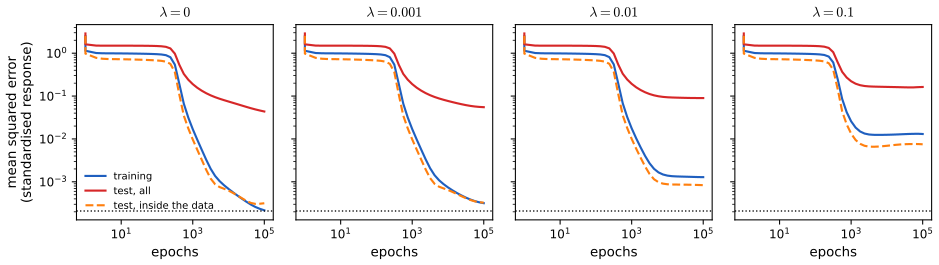
Figure 11.S5 (supplementary, Exercise 11.5(b)). Ten hidden units trained by batch back-propagation (standardised response): training error (blue), test error on all 1000 test points (red) and on the 932 inside the range of the training data along \(a_1\) and \(a_2\) (orange, dashed); dotted: the noise variance. Code: fig_11_s5.(c) Networks with 1–10 units fitted to convergence with \(\lambda=10^{-4}\) (best of five starts; Figure 11.S6, left). On the 932 interior test points the mean squared error (original scale; noise variance 0.09) is 134 with one unit, 0.173 with two, 0.157–0.176 with three to five, and 0.18–0.91 with six to ten (larger networks overfit slightly with this small decay). One unit cannot represent a quadratic (a single sigmoid is monotone); two units can, by facing each other along \(a_2\) to form a U; a third unit would be needed for the sigmoid along \(a_1\), but that term has variance 0.16 and adds little. So two hidden units are the minimum that performs well, and three or four are best.
Exercise 11.6. Write a program for projection pursuit regression with cubic smoothing splines of fixed degrees of freedom. Fit it to the data of Exercise 11.5 for several smoothing parameters and numbers of terms. Find the smallest number of terms that performs well and compare with the number of hidden units of Exercise 11.5.
Solution
The program is
ppr_fit(Section 11.2: forward stagewise terms, the Gauss–Newton step with step halving, backfitting of the ridge functions; smoothers with fixed df). Interior test errors (original scale) for 1–4 terms (Figure 11.S6, right):df 1 term 2 terms 3 terms 4 terms 5 0.99 0.55 0.44 0.35 8 0.31 0.153 0.164 0.157 12 0.29 0.133 0.166 0.203 16 0.31 0.139 0.61 1.31 With enough flexibility (8–16 df) two terms suffice, and they are the two true directions (Figure 11.S2): the model is exactly a sum of two ridge functions, \(\sigma(a_1^\T x)\) and \((a_2^\T x)^2\), whose directions are orthogonal. With 5 df the spline shrinks the quadratic so much that every new term goes back to nearly the same direction to fit what is left (the demonstration, preset 4), and four terms are still not enough; with 16 df the extra terms fit noise. The best PPR fit (0.133) is a little better than the best network (0.157): two flexible ridge functions match the truth, whereas the network needs two sigmoids to make one parabola. The minimum number of terms (2) equals the minimum number of hidden units found in Exercise 11.5, but for different reasons: PPR needs one term per true ridge function, the network one unit per monotone piece.
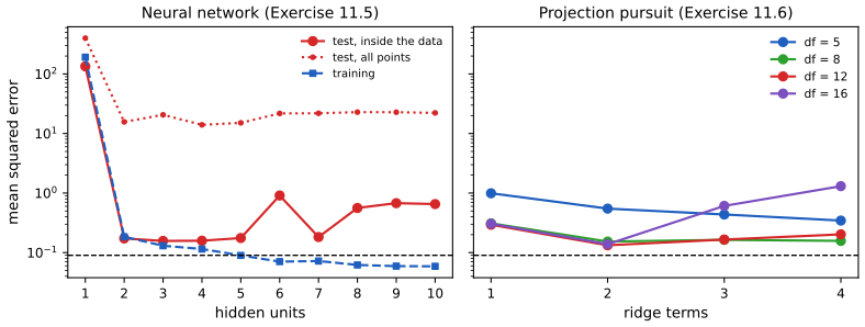
Figure 11.S6 (supplementary, Exercises 11.5(c) and 11.6). Left: networks with 1–10 hidden units (decay \(10^{-4}\), best of five starts): test error inside the data (solid), on all test points (dotted) and training error (dashed). Right: PPR with 1–4 terms and smoothers of 5, 8, 12 and 16 df, test error inside the data. Dashed line: the noise variance 0.09. Code: fig_11_s6.Exercise 11.7. Fit a neural network to the spam data of Section 9.1.2 and compare it with the additive model of that section, both for classification performance and for interpretability.
Solution
Inputs \(\log(x+0.1)\) as in Section 9.1.2, standardised; the book's split (3065 training, 1536 test emails); ten hidden units, softmax outputs, cross-entropy, weight decay chosen by five-fold cross-validation over \(\lambda\in\{0.01,0.1,0.5,1,2,5,10\}\) (602 weights). The CV curve is minimised at \(\lambda=1\) (CV error 4.96%, standard error 0.33%); the network refitted on all the training data with \(\lambda=1\) (best of three starts) has test error 5.27%. The additive logistic model of Section 9.1.2 (a cubic smoothing spline with 4 df for each predictor), fitted with R's
gampackage, has test error 5.47% here (the book reports 5.3%). The difference is far below one standard error of a test error rate, \(\sqrt{0.053\times0.947/1536}=0.57\%\): the two methods classify equally well. Small decay overfits (6.6% at \(\lambda=0.01\)) and large decay underfits (5.9% at 10).For interpretation the additive model wins clearly. Each predictor has one fitted function that is its effect on the log-odds, holding the others fixed. The network has no such components; the closest thing is a partial dependence plot (the average fitted log-odds as one input is varied over the training data). Figure 11.S7 compares them for six predictors: the directions agree (more "!", "$", "remove" and "free" push toward spam, more "hp" and "george" toward email) and the network's curves are smoother and less extreme, but they are averages over the other inputs, they can hide interactions the network has learned, and the 602 weights themselves have no reading. This is the trade-off of Section 11.8: comparable prediction, much less interpretability.
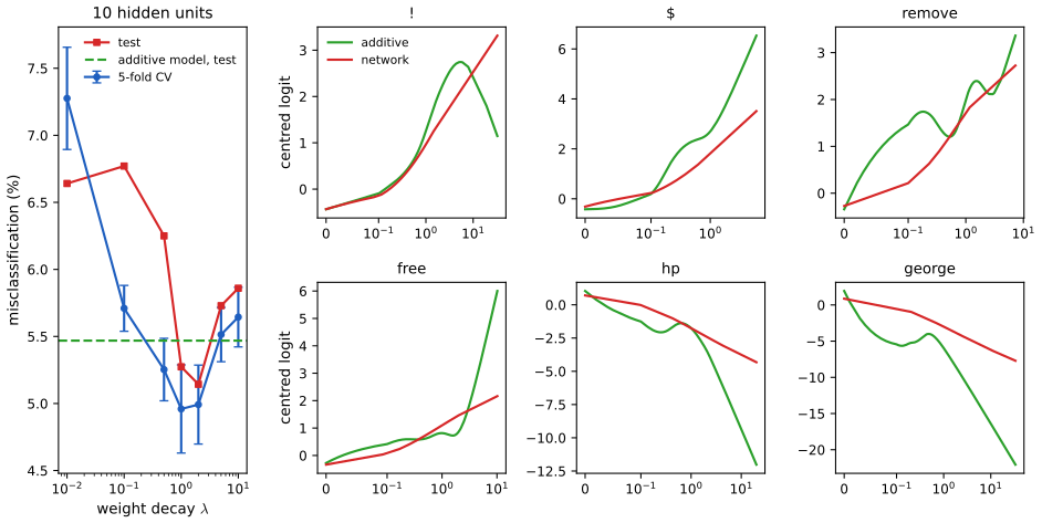
Figure 11.S7 (supplementary, Exercise 11.7). Left: five-fold cross-validation error (with standard errors) and test error of the ten-unit network against the weight decay, and the additive model's test error. Right: for six predictors, the additive model's fitted function (green) and the network's partial dependence (red), both centred, against the raw frequency (symmetric log scale). Code: fig_11_s7.
Demonstrations for this chapter
Each demonstration runs in the browser and links back to these notes. The ▶ Demo boxes above open them already set to the case under discussion.
| Demonstration | What you can see | Sections and results |
|---|---|---|
| Projection pursuit regression | One to three ridge terms on four two-input data sets, with any smoother df, the best of nine starts or a single start at any angle, backfitting on or off: the fitted surface, the fitted directions and the Gauss–Newton path, the partial residuals and ridge functions, and the test error. Presets: 1 a single index model; 2 the product \(x_1x_2\); 3 the Exercise 11.5 model; 4 too few df; 5 greedy stagewise fitting. | 11.2; Results 11.1, 11.2, Filling the gap 11.1, Exercise 11.6 |
| Hidden units, weight decay and random starts | The networks of Section 11.6 fitted in the browser by the quasi-Newton method of nnet: the fitted surface, the norm of every unit's weights, and the boxplots of Figures 11.6–11.8 recomputed over ten starts. Presets: 1 Figure 11.6 (left); 2 no decay; 3 decay 0.1; 4 Figure 11.8; 5 the radial function. | 11.5, 11.6; Results 11.7, 11.9, 11.10 |
| The five ZIP code networks | Net-1 to Net-5 trained on shifted digits and run on 300 test digits: links and weights, all hidden activations, the receptive field of any unit, the shared kernels, the outputs and the test curves. Presets: 1 Net-1; 2 Net-2; 3 local connectivity; 4 shared weights; 5 two levels of sharing. | 11.7; Results 11.11, 11.12 |
Related demonstrations in the companion courses: universal approximation, back-propagation step by step, early stopping and weight decay, committees of networks and a convolutional network on MNIST (Foundations of Deep Learning); back-propagation and a Bayesian network by the Laplace approximation (Bayesian and Probabilistic Machine Learning). The Python code that produces every figure of this page is code/ch11_neural_networks.py (see the code index).
References
- Hastie, T., Tibshirani, R. and Friedman, J. (2009). The Elements of Statistical Learning: Data Mining, Inference, and Prediction, 2nd edition. Springer, New York. Chapter 11, pp. 389–416. hastie.su.domains/ElemStatLearn.
- Barron, A. R. (1993). Universal approximation bounds for superpositions of a sigmoidal function. IEEE Transactions on Information Theory, 39(3), 930–945.
- Bishop, C. M. (1995). Neural Networks for Pattern Recognition. Clarendon Press, Oxford.
- Friedman, J. H. and Stuetzle, W. (1981). Projection pursuit regression. Journal of the American Statistical Association, 76(376), 817–823.
- Friedman, J. H. and Tukey, J. W. (1974). A projection pursuit algorithm for exploratory data analysis. IEEE Transactions on Computers, C-23(9), 881–890.
- Guyon, I., Gunn, S., Nikravesh, M. and Zadeh, L. (eds) (2006). Feature Extraction: Foundations and Applications. Springer, Berlin.
- Hertz, J., Krogh, A. and Palmer, R. G. (1991). Introduction to the Theory of Neural Computation. Addison-Wesley, Redwood City.
- Huber, P. J. (1985). Projection pursuit. The Annals of Statistics, 13(2), 435–475.
- Johnson, N. (2008). A Study of the NIPS Feature Selection Challenge. Technical report, Stanford University.
- Le Cun, Y. (1989). Generalization and network design strategies. In R. Pfeifer et al. (eds), Connectionism in Perspective, 143–155. North-Holland, Amsterdam.
- Le Cun, Y., Bottou, L., Bengio, Y. and Haffner, P. (1998). Gradient-based learning applied to document recognition. Proceedings of the IEEE, 86(11), 2278–2324.
- Nash, J. C. (1990). Compact Numerical Methods for Computers: Linear Algebra and Function Minimisation, 2nd edition. Adam Hilger, Bristol.
- Neal, R. M. (1996). Bayesian Learning for Neural Networks. Springer, New York.
- Neal, R. M. and Zhang, J. (2006). High dimensional classification with Bayesian neural networks and Dirichlet diffusion trees. In Guyon et al. (2006), 265–295.
- Ripley, B. D. (1996). Pattern Recognition and Neural Networks. Cambridge University Press.
- Robbins, H. and Monro, S. (1951). A stochastic approximation method. The Annals of Mathematical Statistics, 22(3), 400–407.
- Roosen, C. B. and Hastie, T. (1994). Automatic smoothing spline projection pursuit. Journal of Computational and Graphical Statistics, 3(3), 235–248.
- Rumelhart, D. E., Hinton, G. E. and Williams, R. J. (1986). Learning internal representations by error propagation. In D. E. Rumelhart and J. L. McClelland (eds), Parallel Distributed Processing, Vol. 1, 318–362. MIT Press, Cambridge, MA.
- Simard, P., Le Cun, Y. and Denker, J. (1993). Efficient pattern recognition using a new transformation distance. In Advances in Neural Information Processing Systems 5, 50–58. Morgan Kaufmann, San Mateo.
- Widrow, B. and Hoff, M. E. (1960). Adaptive switching circuits. IRE WESCON Convention Record, 4, 96–104.
The numerical statements in the text (the polarisation identity, the cubic bound of Result 11.7, the weight-elimination thresholds, the signal variances of Section 11.6, the parameter counts of Table 11.1, the back-propagation gradients, the agreement of the quasi-Newton fits with R's nnet, and the numbers quoted for every figure) were confirmed numerically.