Unsupervised Learning
With no response to predict, the object of study is the joint density of the inputs itself, and the questions become descriptive: where is the density high (association rules, mode seeking), does it split into separate groups (cluster analysis), and does it concentrate near a low-dimensional set (principal components, principal curves, self-organising maps, multidimensional scaling and their nonlinear relatives)? There is no test error to settle disputes, so each method is defined by a criterion, and these notes concentrate on the criteria: what each one measures, why the algorithms that optimise it work, and when their answers can be trusted. The chapter ends with an unexpected relative, the PageRank of web pages, which is the stationary distribution of a random walk.
Ch. 1 Introduction Ch. 2 Supervised learning Ch. 3 Linear regression Ch. 4 Linear classification Ch. 5 Basis expansions Ch. 6 Kernel smoothing Ch. 7 Model assessment Ch. 8 Inference and averaging Ch. 9 Additive models and trees Ch. 10 Boosting Ch. 11 Neural networks Ch. 12 SVMs Ch. 13 Nearest neighbours Ch. 14 Unsupervised learning Ch. 15 Random forests Ch. 16 Ensembles Ch. 17 Graphical models Ch. 18 High-dimensional problems
How to read these notes
They follow the book. Sections carry the book's numbers (14.2, 14.2.1, ...) and every displayed equation that appears in the book carries the book's own equation number, e.g. \((14.33)\), so you can read these notes next to the book. Equations without a number are steps that the book skips.
Filling the gaps. Wherever the book says that something "can be shown", "is easy to show", leaves it to an exercise, or states a property without proof, an orange Filling the gap box or a proof gives the full argument. Proofs and derivations start hidden: open one with its bar, or use the button below.
Figures and demonstrations. The figures computed from data or simulations are reproduced from scratch by the Python code. Where the book's data are not public (a photograph, a corpus of newsgroup articles, face images, brain scans), the same method is applied to data that are, and the caption says so. The ▶ Demo boxes open an interactive demonstration already set to the case being discussed.
A long chapter. The chapter covers some twenty methods. Each section can be read on its own after Section 14.3.6 (K-means) and Section 14.5.1 (principal components), which the others keep returning to.
Main reference
T. Hastie, R. Tibshirani and J. Friedman, The Elements of Statistical Learning: Data Mining, Inference, and Prediction, 2nd edition, Springer (2009), Chapter 14, pages 485–586 (book website, with the data sets: hastie.su.domains/ElemStatLearn). Section, equation, figure, table and exercise numbers below refer to this book. Further reading is listed in the references.
The explanations, derivations, figures and code are my own; equations are cited by their numbers in the book.
Companion courses
Much of this chapter also appears in the three companion courses on this site. The overlapping material is:
- Sections 14.3.6–14.3.7 and 14.3.9 (K-means, its convergence, EM for Gaussian mixtures and the small-variance limit, vector quantisation): Bayesian and Probabilistic Machine Learning, Section 9.1, Filling the gap 9.1, 9.4, Section 9.2.2 and Section 9.3.2; Foundations of Deep Learning, Section 15.1, Result 15.1, Filling the gap 15.2 and Result 15.7.
- Sections 14.3.1–14.3.12 (dissimilarities, K-medoids and PAM, hierarchical clustering, the gap statistic): Statistical Methods for Modern Biology, Section 5.3, Filling the gap 5.6, Section 5.6, Filling the gaps 5.9, 5.10 and 5.13.
- Section 14.5.1 (principal components, the SVD and the best low-rank approximation): Bayesian and Probabilistic Machine Learning, Section 12.1 and Result 12.3; Foundations of Deep Learning, Section 16.1; Statistical Methods for Modern Biology, Theorem 7.4 (Eckart–Young–Mirsky) with its proof.
- Section 14.5.4 (kernel PCA): Section 12.3, Results 12.14 and 12.15.
- Section 14.7 (factor analysis and independent component analysis): Section 12.2.4, Section 12.4.1 and Result 12.16; Foundations of Deep Learning, Sections 16.2.4–16.2.5 and Result 16.10.
- Sections 14.8–14.9 (classical and nonmetric multidimensional scaling, local nonlinear methods): Statistical Methods for Modern Biology, Section 9.2, Theorem 9.2, Result 9.3, Filling the gap 9.5 and Section 9.5.2; Bayesian and Probabilistic Machine Learning, Result 12.18.
Within this course the chapter builds on logistic regression (Section 4.4), natural splines (Section 5.2.1), reproducing kernels (Section 5.8), Gaussian mixtures and the EM algorithm (Section 6.8, Section 8.5), trees and PRIM (Sections 9.2–9.3) and principal components regression (Section 3.5.1). New here: the Apriori algorithm and the reference-density view, the combinatorics of partitions, Lloyd's algorithm and its finite convergence, the gap statistic, the ultrametric of a dendrogram, self-organising maps, Procrustes analysis, principal curves, the graph Laplacian with its zero eigenspace, sparse PCA, non-negative matrix factorisation as a minorise-maximise algorithm, archetypes, the entropy argument behind ICA, local linear embedding, local MDS, and PageRank through the Perron–Frobenius theorem.
The chapter at a glance
- 14.2 Apriori finds every frequent item set because support can only fall as items are added (Result 14.1); classifying data against a reference sample estimates the density ratio \(g/g_0\) (Result 14.2), but against a permuted reference no single split helps (Result 14.3).
- 14.3 The average squared difference is twice the variance (Result 14.4); there are \(S(N,K)\) partitions (Result 14.5); K-means is coordinate descent on the unweighted within-cluster sum of squares and stops in finitely many steps (Result 14.6), and is the small-variance limit of EM (Result 14.7); K-medoids descends on (14.38) (Result 14.8); dendrograms are ultrametrics with non-decreasing heights for single, complete and average linkage (Results 14.9 and 14.10).
- 14.4 With the smallest neighbourhood the SOM is K-means (Result 14.11).
- 14.5 Principal components: partial optimisation (Result 14.12), the best rank-\(q\) approximation (Result 14.13), Procrustes and affine averages (Results 14.14 and 14.15); principal curves with a linear smoother are the power method (Result 14.16); the Laplacian's quadratic form and its zero eigenspace (Results 14.17 and 14.18); kernel PCA through the Gram matrix and in the RKHS (Results 14.19 and 14.20); sparse PCA without the lasso penalty is PCA (Result 14.21).
- 14.6 The NMF updates are a minorise-maximise algorithm (Result 14.22); archetypes lie on the convex hull (Result 14.23).
- 14.7 Entropy, mutual information and why ICA maximises non-Gaussianity (Result 14.24); the ProDenICA density has mean 0 and variance 1 (Result 14.25).
- 14.8–14.9 Classical scaling is PCA (Result 14.26); the two LLE steps in closed form (Result 14.27).
- 14.10 PageRank exists, is unique and positive, and the power method converges at rate \(d\) (Result 14.28).
Notes on the book in this chapter: the number of rules and a lift, what K-means minimises, the responsibilities in Figure 14.7, Table 14.2, the noise level of the half-sphere data, the location in (14.57), the two PageRank normalisations and (14.122).
Notation. Data \(x_1,\dots,x_N\in\R^p\), stacked as the rows of the \(N\times p\) matrix \(\bX\) (centred where stated); \(d_{ii'}\) a dissimilarity; \(C(i)\) the cluster of observation \(i\), \(N_k\) the size and \(\bar x_k\) the mean of cluster \(k\); \(\bX=\bU\bD\bV^\T\) the singular value decomposition with \(d_1\ge d_2\ge\cdots\); \(\bW\) is a weight matrix (graph adjacencies, NMF or LLE weights) whose meaning is fixed in each section; \(\bone\) and \(\be\) are vectors of ones; \(\|\cdot\|_F\) is the Frobenius norm.
Prerequisites. The singular value decomposition, Lagrange multipliers, the EM algorithm (Section 8.5), reproducing kernels (Section 5.8) and basic Markov chains.
14.1 Introduction
pp. 485–487 In supervised learning the training data are pairs \((x_i,y_i)\) and the target is a property of the conditional density \(\Pr(Y\given X)\), usually a location such as
\[ \mu(x)=\argmin_\theta \E_{Y|X}L(Y,\theta). \tag{14.1} \]Because \(\Pr(X,Y)=\Pr(Y\given X)\Pr(X)\), supervised learning ignores the marginal \(\Pr(X)\). In unsupervised learning there is only a sample \(x_1,\dots,x_N\) of a random \(p\)-vector \(X\), and \(\Pr(X)\) is the object of study. In low dimensions (\(p\le3\), say) it can be estimated directly by the kernel methods of Chapter 6; in high dimensions the curse of dimensionality forces cruder summaries: where the density is large (association rules, Section 14.2; mode seeking), whether it is a mixture of separated pieces (cluster analysis, Section 14.3), or whether it concentrates near a low-dimensional manifold (principal components, curves and surfaces, self-organising maps, multidimensional scaling, Sections 14.4–14.9).
Filling the gap 14.1: what (14.1) is for the common losses, and why there is no test error here pp. 485–487
Derivation
For squared error, \(\E[(Y-\theta)^2\given X=x]=\Var(Y\given x)+(\E[Y\given x]-\theta)^2\) is minimised at \(\theta=\E(Y\given x)\); for absolute error \(\E|Y-\theta|\) has derivative \(\Pr(Y\lt\theta\given x)-\Pr(Y>\theta\given x)\) in \(\theta\), which changes sign at the conditional median. In both cases the target is a single number per \(x\), and its quality is judged by the expected loss \(\E\,L(Y,\hat\mu(X))\) over the joint distribution, which can be estimated on new data or by cross-validation (Chapter 7).
In the unsupervised problem there is no \(Y\) and so no loss with a "correct answer". One could judge a density estimate \(\hat g\) by the expected log-likelihood \(\E\log\hat g(X)\) on new data, and Section 14.2.4 turns density estimation into a classification problem that can be cross-validated; but most methods of this chapter produce descriptive summaries (clusters, directions, maps) whose criteria, such as the within-cluster scatter, keep improving as the summary gets richer, on training data and on new data alike (Filling the gap 14.8). That is the "uncomfortable situation" the book describes, and the reason so many methods coexist. ∎
14.2 Association Rules
pp. 487–488 The general goal is to find values \(v_1,\dots,v_L\) where the density \(\Pr(v_l)\) is large ("mode finding" or "bump hunting"). Estimating \(\Pr(X=v)\) by the fraction of observations equal to \(v\) is hopeless once \(p\) is moderate: almost every \(v\) is observed at most once. The first simplification looks instead for regions of high probability. Let \(\mathcal{S}_j\) be the set of possible values of \(X_j\) and \(s_j\subseteq\mathcal{S}_j\). The aim becomes to find subsets \(s_1,\dots,s_p\) for which
\[ \Pr\Big[\bigcap_{j=1}^p(X_j\in s_j)\Big] \tag{14.2} \]is large. Such an intersection is a conjunctive rule; when \(s_j=\mathcal{S}_j\) the variable \(X_j\) does not appear in the rule.
14.2.1 Market Basket Analysis
pp. 488–489 For commercial data bases (\(p\approx10^4\), \(N\approx10^8\)) a second simplification is needed: each \(s_j\) is either a single value \(v_{0j}\) or the whole of \(\mathcal{S}_j\). The problem is then to find \(\mathcal{J}\subset\{1,\dots,p\}\) and values \(v_{0j}\), \(j\in\mathcal{J}\), with
\[ \Pr\Big[\bigcap_{j\in\mathcal{J}}(X_j=v_{0j})\Big] \tag{14.3} \]large. Coding every value of every variable as a dummy variable \(Z_k\) (\(K=\sum_j|\mathcal{S}_j|\) of them) turns (14.3) into a problem on binary variables: find \(\Kc\subset\{1,\dots,K\}\) with
\[ \Pr\Big[\bigcap_{k\in\Kc}(Z_k=1)\Big]=\Pr\Big[\prod_{k\in\Kc}Z_k=1\Big] \tag{14.4} \]large. This is the market basket problem: \(Z_k=1\) if item \(k\) is in the basket.
Definition 14.1 (item sets, support, confidence, lift) pp. 489–491, (14.5)–(14.9)
A set \(\Kc\) of items is an item set; \(|\Kc|\) is its size. Its support (prevalence) is the fraction of baskets that contain it,
\[ T(\Kc)=\widehat\Pr\Big[\prod_{k\in\Kc}Z_k=1\Big]=\frac1N\sum_{i=1}^N\prod_{k\in\Kc}z_{ik}. \tag{14.5} \]Given a threshold \(t\), the target is the collection of frequent item sets
\[ \{\Kc_l\given T(\Kc_l)>t\}. \tag{14.6} \]An item set \(\Kc\) is split into disjoint non-empty parts \(A\cup B=\Kc\), written as the association rule
\[ A\Rightarrow B, \tag{14.7} \]with antecedent \(A\) and consequent \(B\). The rule's support is \(T(A\Rightarrow B)=T(\Kc)\), an estimate of \(\Pr(A\text{ and }B)\); its confidence (predictability) is
\[ C(A\Rightarrow B)=\frac{T(A\Rightarrow B)}{T(A)}, \tag{14.8} \]an estimate of \(\Pr(B\given A)\); its expected confidence is \(T(B)\), an estimate of \(\Pr(B)\); and its lift is \(L(A\Rightarrow B)=C(A\Rightarrow B)/T(B)\), an estimate of \(\Pr(A\text{ and }B)/[\Pr(A)\Pr(B)]\). Lift 1 means that \(A\) and \(B\) occur together as often as they would if they were independent. Rules are reported if their confidence also exceeds a threshold \(c\):
\[ \{A\Rightarrow B\given C(A\Rightarrow B)>c\}. \tag{14.9} \]14.2.2 The Apriori Algorithm
pp. 489–492 There are \(2^K\) item sets, far too many to count. Apriori (Agrawal et al., 1995) finds all of (14.6) in one pass over the data per item-set size, using two facts: for a reasonable \(t\) the collection (14.6) is small, and support can only fall when items are added.
Result 14.1 (support is anti-monotone, and Apriori finds every frequent item set) p. 490
(a) If \(\mathcal{L}\subseteq\Kc\) then \(T(\mathcal{L})\ge T(\Kc)\).
(b) Let \(F_m\) be the frequent item sets of size \(m\). Apriori forms the candidates of size \(m+1\) from those \(\Kc\cup\{k\}\), \(\Kc\in F_m\), \(\{k\}\in F_1\), all of whose \(m+1\) subsets of size \(m\) are in \(F_m\), counts their support in one pass, and keeps the frequent ones. Then every frequent item set of size \(m+1\) is a candidate, so the algorithm returns exactly (14.6), and it stops after at most (largest frequent size) + 1 passes.
Proof
(a) A basket that contains every item of \(\Kc\) contains every item of \(\mathcal{L}\): \(\prod_{k\in\Kc}z_{ik}\le\prod_{k\in\mathcal{L}}z_{ik}\) for each \(i\), because the extra factors are 0 or 1. Average over \(i\).
(b) Let \(\Kc'\) be frequent with \(|\Kc'|=m+1\). By (a) each of its subsets of size \(m\) has support at least \(T(\Kc')>t\), so all of them are in \(F_m\), and each single item of \(\Kc'\) is in \(F_1\). Removing the largest item \(k\) of \(\Kc'\) gives \(\Kc=\Kc'\setminus\{k\}\in F_m\), so \(\Kc'=\Kc\cup\{k\}\) is generated and survives the subset test. Since only candidates are counted and each is counted exactly, the frequent sets found at size \(m+1\) are exactly \(F_{m+1}\); by induction from \(F_1\) (one full pass) all of (14.6) is found. If \(F_m\) is empty no candidate of size \(m+1\) exists, and by (a) neither does any larger frequent set, so stopping is correct. ∎
The rules (14.9) follow from the frequent sets alone: \(C(A\Rightarrow B)=T(\Kc)/T(A)\) and \(A\subset\Kc\) is itself frequent by (a), so its support is already known and no further pass over the data is needed.
Note on the book: the number of rules from one item set, and the lift in the example p. 491
Rules. The book says an item set of size \(|\Kc|\) gives \(2^{|\Kc|-1}-1\) rules \(A\Rightarrow(\Kc-A)\). The antecedent can be any non-empty proper subset of \(\Kc\), and \(A\Rightarrow B\) and \(B\Rightarrow A\) are different rules (with different confidences), so the count is \(2^{|\Kc|}-2\). For \(\Kc=\{a,b\}\) the two rules are \(\{a\}\Rightarrow\{b\}\) and \(\{b\}\Rightarrow\{a\}\), while \(2^{1}-1=1\). The book's number counts unordered splits \(\{A,B\}\).
Lift. In the peanut butter example, confidence 0.82 and \(T(\text{bread})=0.43\) give lift \(0.82/0.43=1.91\), not 1.95.
14.2.3 Example: Market Basket Analysis
pp. 492–495 The demographics data (Table 14.1 in the book) are answers to 14 questions from 9409 shopping-mall questionnaires (the book's website has the 8993 with income recorded). Removing incomplete rows leaves 6876 observations, as in the book. Each of the six ordinal inputs (income, age, education, years in the Bay Area, household size, number of children) is cut at its median into two dummies, and each of the eight categorical inputs with \(k\) categories gives \(k\) dummies: 50 dummies in all, matching the book's \(6876\times50\) matrix.
Our implementation of Apriori (apriori), with support at least 10%, item sets of at most five items and rules with confidence at least 80% and one consequent item, finds 4925 frequent item sets and 6343 rules (the book reports 6288 rules with an external implementation; the coding details of the median cut account for the difference). Figure 14.2 compares how often each dummy appears in the data and in the rules.
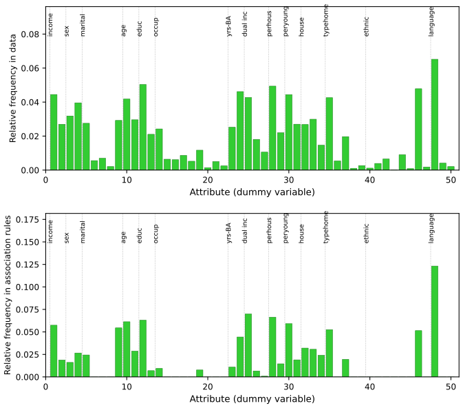
fig_14_2. Reproduces Hastie, Tibshirani and Friedman (2009), Figure 14.2. Download: PDF · SVGThree rules from our list illustrate the three measures:
- {white} \(\Rightarrow\) {English at home}: support 66.0%, confidence 98.5%, lift 1.08. Very common, and barely more frequent than under independence.
- {education up to some college} \(\Rightarrow\) {English at home}: support 63.4%, confidence 90.0%, lift 0.99. A high confidence says nothing by itself: this rule has negative association, since English is spoken in 91% of all households.
- {single, children at home, lives in a house} \(\Rightarrow\) {lives with parents or family}: support 10.7%, confidence 87.6%, lift 4.27. The highest lift in the list, a genuine association.
The book's second example rule has the high-income dummy as consequent; ours with the highest confidence is {married, professional or managerial, owns the home} \(\Rightarrow\) {income above the median}, with support 10.4%, confidence 87.5% and lift 2.32. If only associations with a rare item's presence are wanted (high income, not low income), only that item's dummy should be included.
14.2.4 Unsupervised as Supervised Learning
pp. 495–497 Let \(g\) be the unknown density of the data and \(g_0\) a reference density that we choose and can sample from (for instance uniform on the range of the data). Draw \(N_0\) points from \(g_0\), label the data \(Y=1\) and the reference sample \(Y=0\), and give weight \(w=N_0/(N+N_0)\) to each data point and \(w_0=N/(N+N_0)\) to each reference point. Then
\[ \mu(x)=\E(Y\given x)=\frac{g(x)}{g(x)+g_0(x)}=\frac{g(x)/g_0(x)}{1+g(x)/g_0(x)} \tag{14.10} \]can be estimated from the pooled sample
\[ (y_1,x_1),(y_2,x_2),\dots,(y_{N+N_0},x_{N+N_0}) \tag{14.11} \]by any classifier, and inverted to give
\[ \hat g(x)=g_0(x)\frac{\hat\mu(x)}{1-\hat\mu(x)}. \tag{14.12} \]Logistic regression estimates the log-odds
\[ f(x)=\log\frac{g(x)}{g_0(x)} \tag{14.13} \]directly, and then
\[ \hat g(x)=g_0(x)\,e^{\hat f(x)}. \tag{14.14} \]Result 14.2 (classification against a reference sample estimates the density ratio) p. 495, (14.10)–(14.14)
With the weights above, the weighted pooled sample is a sample from the equal mixture \(\tfrac12(g+g_0)\), and \(\Pr(Y=1\given x)=g(x)/[g(x)+g_0(x)]\) whatever \(N_0\) is. Without the weights, \(\Pr(Y=1\given x)=Ng(x)/[Ng(x)+N_0g_0(x)]\) and the log-odds are \(\log[g(x)/g_0(x)]+\log(N/N_0)\): an intercept shift, which any logistic regression with an intercept absorbs.
Proof
Pick one point of the pooled sample with probability proportional to its weight. The total weight of the data points is \(N\cdot N_0/(N+N_0)\) and that of the reference points is \(N_0\cdot N/(N+N_0)\): the same. So the chosen point comes from \(g\) or \(g_0\) with probability \(\tfrac12\) each and has density \(\tfrac12g+\tfrac12g_0\); by Bayes' theorem
\[ \Pr(Y=1\given x)=\tfrac12g(x)/[\tfrac12g(x)+\tfrac12g_0(x)], \]which is (14.10). Solving \(\mu=r/(1+r)\) for \(r=g/g_0\) gives \(r=\mu/(1-\mu)\), hence (14.12), and \(\log r=\log[\mu/(1-\mu)]\) is the logit, hence (14.13)–(14.14). Without weights the prior class probabilities are \(N/(N+N_0)\) and \(N_0/(N+N_0)\), and the same calculation gives the stated form. ∎
Both \(\mu\) and \(f\) are increasing functions of \(g/g_0\), so their contours are contours of the density ratio, and (when \(g_0\) is uniform) of \(\hat g\) itself. With a product-of-marginals reference the ratio is the dependence density \(g(x)/\prod_jg_j(x_j)\), which equals 1 everywhere exactly when the variables are independent.
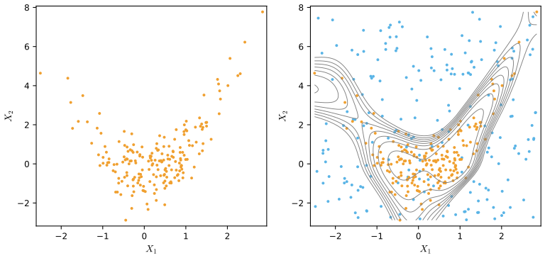
fig_14_3, density_by_classification. Reproduces Hastie, Tibshirani and Friedman (2009), Figure 14.3. Download: PDF · SVGThe choice of \(g_0\) decides what "interesting" means: the uniform for departures from uniformity, a Gaussian with the data's mean and covariance for departures from normality, and the product of the marginal densities
\[ g_0(x)=\prod_{j=1}^p g_j(x_j) \tag{14.15} \]for departures from independence. A sample from (14.15) is made by permuting each column of the data matrix independently.
Filling the gap 14.2: why independent column permutations sample the product of the marginals p. 497
Derivation
Let \(\pi_1,\dots,\pi_p\) be independent uniformly random permutations of \(\{1,\dots,N\}\) and form the reference row \(i\) as \((x_{\pi_1(i)1},\dots,x_{\pi_p(i)p})\). For a fixed \(i\), \(\pi_j(i)\) is uniform on \(\{1,\dots,N\}\) and the \(\pi_j(i)\) are independent across \(j\), so the reference row is a draw from \(\prod_j\hat G_j\), the product of the empirical marginal distributions. Different rows are not independent (they are sampled without replacement), but every reference column has exactly the data's multiset of values: the marginal distributions match perfectly, and all the dependence between variables is destroyed. That exact match has a consequence for tree methods, Result 14.3.
14.2.5 Generalized Association Rules
pp. 497–499 Back to the general problem (14.2), now with intervals for quantitative variables and arbitrary subsets of categories: find \(\mathcal{J}\) and \(s_j\), \(j\in\mathcal{J}\), with large
\[ \widehat\Pr\Big[\bigcap_{j\in\mathcal{J}}(X_j\in s_j)\Big]=\frac1N\sum_{i=1}^N I\Big[\bigcap_{j\in\mathcal{J}}(x_{ij}\in s_j)\Big]. \tag{14.16} \]An exhaustive search is impossible and heuristics are needed. Both (14.5) and (14.16) implicitly compare with the uniform distribution, and so favour sets whose marginal pieces are individually frequent, that is with large
\[ \frac1N\sum_{i=1}^NI(x_{ij}\in s_j). \tag{14.17} \]This is why a high-lift but low-support rule such as vodka \(\Rightarrow\) caviar is never found. Using the product reference (14.15) removes the preference: if the variables were independent the ratio \(g/g_0\) would be flat, whatever the marginal frequencies. With a reference sample in hand, the task becomes a supervised one: find regions
\[ R=\bigcap_{j\in\mathcal{J}}(X_j\in s_j) \tag{14.18} \]where \(\mu(x)=\E(Y\given x)\) is large, with data support
\[ T(R)=\int_{x\in R}g(x)\,dx \tag{14.19} \]not too small.
14.2.6 Choice of Supervised Learning Method
p. 499 The regions (14.18) are conjunctive rules, so methods that output such rules are natural: the terminal nodes of a CART tree (Section 9.2) with high average \(\bar y_t\), whose data support is \(\hat T(R_t)=\bar y_tN_t/N\) (\(N_t\) pooled observations in the node), or the boxes of PRIM (Section 9.3), which aim directly at high-mean, high-support regions. Exercise 14.3 points to a snag.
Result 14.3 (against a permutation reference, no first split helps; Exercise 14.3) p. 499
If the reference sample is made by permuting each column of the data (Filling the gap 14.2), then every region defined by one variable, \(\{X_j\in s\}\), contains equally many data and reference points. Hence every candidate first split of CART has class proportion exactly \(\tfrac12\) in both children and zero impurity decrease, and every first peel of PRIM leaves the box mean at exactly \(\tfrac12\).
Proof
The data column \(j\) and the reference column \(j\) are the same multiset of values, so \(\#\{i:x_{ij}\in s\}\) is the same in both samples for every \(s\). A child of a split on \(X_j\) is such a region; its class-1 fraction is \(n/(n+n)=\tfrac12\), equal to the root's, and any impurity function (Gini, deviance, misclassification) gives the same value in the children as in the root, so the decrease is 0. PRIM's peels on a single variable are regions of the same kind. ∎
On the demographics data, a tree fitted to the 6876 questionnaires against their permuted copy indeed has a first split with Gini decrease exactly 0 (our market_tree): the first split is chosen by an arbitrary tie-break. The associations are visible only jointly, two variables at a time, and a greedy one-variable search cannot see the first step. Remedies are in the solution to Exercise 14.3.
14.2.7 Example: Market Basket Analysis (Continued)
pp. 499–501 The book applies PRIM to the demographics data against the product reference and lists generalised item sets with support 15–24% and rules with confidence above 95%, for example {householder status = rent, type of home \(\ne\) house} \(\Rightarrow\) {marital status = single or living together}; rules involving "type of home \(\ne\) apartment" are out of reach of Apriori, which can only use the dummies it is given. Apriori is exhaustive for its restricted class; PRIM (or CART) is greedy over a much larger class. Exercise 14.4 repeats the analysis with a classification tree.
14.3 Cluster Analysis
pp. 501–503 Cluster analysis (segmentation) groups objects so that objects in the same group are more alike than objects in different groups, sometimes as a hierarchy of nested groups, sometimes to decide whether the data consist of distinct subpopulations at all. Everything depends on the notion of (dis)similarity, which must come from the subject matter, much as the loss function does in prediction.
See also (companion course): Statistical Methods for Modern Biology, Chapter 5, on clustering biological data.
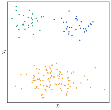
fig_14_4. Reproduces Hastie, Tibshirani and Friedman (2009), Figure 14.4. Download: PDF · SVGK-means, used for Figure 14.4, alternates two steps from a guess of the centres: assign each point to the closest centre; replace each centre by the mean of its points. It is a top-down method; hierarchical methods (Section 14.3.12) work bottom-up.
14.3.1 Proximity Matrices
p. 503 Sometimes the data are an \(N\times N\) matrix \(\bD\) of judged dissimilarities \(d_{ii'}\) (for example averages of subjects' ratings). Most algorithms want \(d_{ii'}\ge0\), \(d_{ii}=0\) and symmetry; a non-symmetric \(\bD\) is replaced by \((\bD+\bD^\T)/2\). Judged dissimilarities rarely satisfy the triangle inequality \(d_{ii'}\le d_{ik}+d_{i'k}\), so methods that assume a metric cannot be used.
Filling the gap 14.3: \((\bD+\bD^\T)/2\) is the closest symmetric matrix p. 503
Derivation
Write \(\bD=\bS+\bA\) with \(\bS=(\bD+\bD^\T)/2\) symmetric and \(\bA=(\bD-\bD^\T)/2\) antisymmetric. For any symmetric \(\bM\), \(\Tr[(\bS-\bM)^\T\bA]=0\) because the trace of a symmetric matrix times an antisymmetric one vanishes (
\[ \Tr(\bP\bA)=\Tr((\bP\bA)^\T)=\Tr(\bA^\T\bP)=-\Tr(\bA\bP)=-\Tr(\bP\bA) \]). Hence \(\|\bD-\bM\|_F^2=\|\bS-\bM\|_F^2+\|\bA\|_F^2\), minimised over symmetric \(\bM\) at \(\bM=\bS\). The symmetrised matrix keeps nonnegativity and a zero diagonal. ∎
14.3.2 Dissimilarities Based on Attributes
pp. 503–505 With measurements \(x_{ij}\) on \(p\) attributes, one defines a dissimilarity \(d_j(x_{ij},x_{i'j})\) per attribute and adds them up:
\[ D(x_i,x_{i'})=\sum_{j=1}^p d_j(x_{ij},x_{i'j}). \tag{14.20} \]The usual choice is squared difference
\[ d_j(x_{ij},x_{i'j})=(x_{ij}-x_{i'j})^2. \tag{14.21} \]Quantitative variables. Any increasing function of \(|x_i-x_{i'}|\) can be used; squared error stresses large differences more than absolute error. Alternatively one can use the correlation across variables
\[ \rho(x_i,x_{i'})=\frac{\sum_j(x_{ij}-\bar x_i)(x_{i'j}-\bar x_{i'})}{\sqrt{\sum_j(x_{ij}-\bar x_i)^2\sum_j(x_{i'j}-\bar x_{i'})^2}}, \tag{14.22} \]with \(\bar x_i=\sum_jx_{ij}/p\), an average over variables, not observations.
Filling the gap 14.4: correlation similarity is squared distance between standardised profiles p. 504
Derivation
Standardise each observation across its variables: \(\tilde x_{ij}=(x_{ij}-\bar x_i)/s_i\) with \(s_i^2=\frac1p\sum_j(x_{ij}-\bar x_i)^2\), so that \(\sum_j\tilde x_{ij}=0\) and \(\sum_j\tilde x_{ij}^2=p\). Then (14.22) is \(\rho(x_i,x_{i'})=\frac1p\sum_j\tilde x_{ij}\tilde x_{i'j}\), and
\[ \sum_{j=1}^p(\tilde x_{ij}-\tilde x_{i'j})^2=\sum_j\tilde x_{ij}^2+\sum_j\tilde x_{i'j}^2-2\sum_j\tilde x_{ij}\tilde x_{i'j}=2p\,\big[1-\rho(x_i,x_{i'})\big]. \]So ranking pairs by large correlation is ranking them by small squared distance between standardised profiles, and any clustering criterion based on one is based on the other. This is the "standardisation" meant in the book: of observations across variables, not of variables across observations. ∎
Ordinal variables (grades, preference scales, ranks) with \(M\) ordered values are replaced by
\[ \frac{i-1/2}{M},\quad i=1,\dots,M, \tag{14.23} \]in their order, and then treated as quantitative. These are the midpoints of \(M\) equal bins of \([0,1]\), so the scale runs from \(1/(2M)\) to \(1-1/(2M)\) whatever \(M\) is. Categorical variables with \(M\) values need an explicit \(M\times M\) loss matrix \(L_{rr'}=L_{r'r}\ge0\), \(L_{rr}=0\); the usual choice is \(L_{rr'}=1\) for \(r\ne r'\).
14.3.3 Object Dissimilarity
pp. 505–507 The attribute dissimilarities are combined by a convex combination
\[ D(x_i,x_{i'})=\sum_{j=1}^pw_j\cdot d_j(x_{ij},x_{i'j});\qquad\sum_{j=1}^pw_j=1. \tag{14.24} \]Equal weights do not give equal influence. The influence of attribute \(j\) on the average dissimilarity over all pairs is \(w_j\bar d_j\), with
\[ \bar d_j=\frac1{N^2}\sum_{i=1}^N\sum_{i'=1}^Nd_j(x_{ij},x_{i'j}) \tag{14.25} \]the average dissimilarity on attribute \(j\), so \(w_j\propto1/\bar d_j\) equalises the influences. For squared differences (14.24) is the weighted squared Euclidean distance
\[ D_I(x_i,x_{i'})=\sum_{j=1}^pw_j\cdot(x_{ij}-x_{i'j})^2 \tag{14.26} \]and (14.25) becomes
\[ \bar d_j=\frac1{N^2}\sum_{i=1}^N\sum_{i'=1}^N(x_{ij}-x_{i'j})^2=2\cdot\mathrm{var}_j. \tag{14.27} \]Result 14.4 (the average squared difference is twice the variance) p. 505, (14.27)
With \(\mathrm{var}_j=\frac1N\sum_i(x_{ij}-\bar x_j)^2\) (divisor \(N\)), \(\frac1{N^2}\sum_{i,i'}(x_{ij}-x_{i'j})^2=2\,\mathrm{var}_j\). Hence equal influence for squared distance means \(w_j\propto1/\mathrm{var}_j\), which is standardising every variable.
Proof
Write \(a_i=x_{ij}-\bar x_j\), so \(\sum_ia_i=0\). Then
\[ \sum_{i,i'}(a_i-a_{i'})^2=\sum_{i,i'}(a_i^2+a_{i'}^2)-2\sum_ia_i\sum_{i'}a_{i'}=2N\sum_ia_i^2, \]and dividing by \(N^2\) gives \(2\cdot\frac1N\sum_ia_i^2\). ∎
Equalising influence is often recommended and often harmful: if one variable carries the grouping, giving every variable the same influence dilutes it. Figure 14.5 shows this.
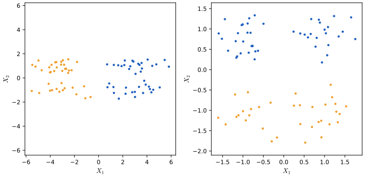
fig_14_5. Reproduces Hastie, Tibshirani and Friedman (2009), Figure 14.5. Download: PDF · SVGFilling the gap 14.5: when standardising hides the groups p. 506
Derivation
For two clusters split along one coordinate, the K-means criterion (per point, standardised data) is roughly the total variance of the other coordinate, 1, plus the within-half variance of the split coordinate, \(r_j\le1\), the fraction of the variance of \(X_j\) left inside the two halves. Splitting \(X_1\) costs \(1+r_1\), splitting \(X_2\) costs \(r_2+1\): K-means splits the variable whose two halves are relatively tighter. In Figure 14.5, \(r_1=1.2^2/(3^2+1.2^2)\approx0.14\) and \(r_2\approx0.35^2/(1+0.35^2)\approx0.11\), so after standardising, \(X_2\) wins, although on the raw scale the \(X_1\) split reduces the sum of squares by about 36 units per point and the \(X_2\) split by less than 1. Standardising replaces "how much variance is explained" by "how bimodal is each variable", which may or may not be the question of interest. ∎
Missing values are usually handled by omitting, in (14.24), the attributes missing in either object; imputation, or treating "missing" as a category, are alternatives.
14.3.4 Clustering Algorithms
p. 507 Three families: combinatorial algorithms work on the data (or dissimilarities) directly; mixture modelling fits a parametric mixture density by maximum likelihood (Section 6.8); mode seekers (bump hunters, such as PRIM) estimate the modes of the density nonparametrically.
14.3.5 Combinatorial Algorithms
pp. 507–508 An encoder \(k=C(i)\) assigns each of the \(N\) observations to one of \(K\lt N\) clusters. A natural loss is the within-cluster point scatter
\[ W(C)=\frac12\sum_{k=1}^K\sum_{C(i)=k}\sum_{C(i')=k}d(x_i,x_{i'}). \tag{14.28} \]With the total scatter \(T=\frac12\sum_i\sum_{i'}d_{ii'}\) and the between-cluster scatter
\[ B(C)=\frac12\sum_{k=1}^K\sum_{C(i)=k}\sum_{C(i')\ne k}d_{ii'}, \tag{14.29} \]one has \(T=W(C)+B(C)\): every ordered pair is either within a cluster or between clusters. \(T\) does not depend on \(C\), so minimising \(W\) is maximising \(B\). Complete enumeration is out of reach; the number of distinct assignments is
\[ S(N,K)=\frac1{K!}\sum_{k=1}^K(-1)^{K-k}\binom Kk k^N. \tag{14.30} \]Result 14.5 (the number of partitions into \(K\) non-empty clusters) p. 508, (14.30)
\(S(N,K)\) in (14.30), the Stirling number of the second kind, is the number of ways to partition \(N\) labelled objects into \(K\) non-empty unlabelled groups. \(S(10,4)=34{,}105\) and \(S(19,4)=11{,}259{,}666{,}950\approx10^{10}\); for fixed \(K\), \(S(N,K)\sim K^N/K!\).
Proof
Count maps \(c:\{1,\dots,N\}\to\{1,\dots,K\}\) that are onto. There are \(K^N\) maps in all. Let \(A_m\) be the set of maps that miss value \(m\). By inclusion–exclusion the number of onto maps is \(\sum_{j=0}^K(-1)^j\binom Kj(K-j)^N\), since the maps missing a given set of \(j\) values are the \((K-j)^N\) maps into the other \(K-j\). Substituting \(k=K-j\) gives \(\sum_{k=0}^K(-1)^{K-k}\binom Kkk^N\), and the \(k=0\) term vanishes for \(N\ge1\). An onto map is an encoder that uses every label; permuting the labels gives the same partition, and the \(K!\) permutations give distinct maps, so dividing by \(K!\) counts partitions. The two values are direct evaluations, and as \(N\to\infty\) the \(k=K\) term dominates because \((k/K)^N\to0\) for \(k\lt K\). ∎
Practical algorithms are greedy descents: start from a partition and change assignments so as to improve the criterion until no change helps. They examine a tiny fraction of the \(S(N,K)\) partitions and stop at a local optimum.
14.3.6 K-means
pp. 509–510 K-means is for quantitative variables with squared Euclidean distance
\[ d(x_i,x_{i'})=\sum_j(x_{ij}-x_{i'j})^2=\|x_i-x_{i'}\|^2 \](weighted distances reduce to this by rescaling the variables, Exercise 14.1). The within-point scatter (14.28) can be written as
\[ W(C)=\frac12\sum_{k=1}^K\sum_{C(i)=k}\sum_{C(i')=k}\|x_i-x_{i'}\|^2=\sum_{k=1}^KN_k\sum_{C(i)=k}\|x_i-\bar x_k\|^2, \tag{14.31} \]with \(\bar x_k\) the mean of cluster \(k\) and \(N_k\) its size. For any set \(S\) of observations
\[ \bar x_S=\argmin_m\sum_{i\in S}\|x_i-m\|^2, \tag{14.32} \]so the book writes the problem as the enlarged minimisation
\[ \min_{C,\{m_k\}_1^K}\sum_{k=1}^KN_k\sum_{C(i)=k}\|x_i-m_k\|^2. \tag{14.33} \]Algorithm 14.1 K-means clustering p. 510
- For the current assignment \(C\), replace each centre \(m_k\) by the mean of the observations assigned to cluster \(k\) (14.32).
- For the current centres, assign each observation to the closest one: \[ C(i)=\argmin_{1\le k\le K}\|x_i-m_k\|^2. \tag{14.34} \]
- Repeat until the assignments do not change.
See also (companion courses): Bayesian and Probabilistic Machine Learning, Filling the gap 9.1; Foundations of Deep Learning, Result 15.1; Statistical Methods for Modern Biology, Filling the gap 5.5.
Result 14.6 (what K-means minimises, and why it stops) pp. 509–510, (14.31)–(14.34)
(a) The identity (14.31) holds, and (14.32) holds with a unique minimiser.
(b) Algorithm 14.1 is coordinate descent on the unweighted criterion
\[ J(C,\{m_k\})=\sum_{k=1}^K\sum_{C(i)=k}\|x_i-m_k\|^2, \]whose minimum over the centres is
\[ \min_{\{m_k\}}J(C,\{m_k\})=\sum_{k=1}^K\sum_{C(i)=k}\|x_i-\bar x_k\|^2=\sum_{k=1}^K\frac{1}{2N_k}\sum_{C(i)=k}\sum_{C(i')=k}\|x_i-x_{i'}\|^2 . \]Each step does not increase \(J\); with ties in (14.34) broken by keeping the current cluster, \(J\) decreases strictly at every iteration that changes the assignment, so no partition is visited twice and the algorithm stops after finitely many iterations (at most \(S(N,K)\)), at a partition where no single step of either kind improves \(J\).
Proof
(14.32). For any \(m\),
\[ \sum_{i\in S}\|x_i-m\|^2=\sum_{i\in S}\|x_i-\bar x_S\|^2+|S|\,\|\bar x_S-m\|^2, \]because the cross term \(2(\bar x_S-m)^\T\sum_{i\in S}(x_i-\bar x_S)\) vanishes. The second term is zero only at \(m=\bar x_S\).
(14.31). Apply the same decomposition with \(m=x_{i'}\) and sum over \(i'\in S\):
\[ \sum_{i'}\sum_i\|x_i-x_{i'}\|^2=\sum_{i'}\big[\sum_i\|x_i-\bar x_S\|^2+|S|\|\bar x_S-x_{i'}\|^2\big]=2|S|\sum_i\|x_i-\bar x_S\|^2. \]Halve and sum over clusters.
(b) Step 1 minimises \(J\) over the centres for fixed \(C\) by (14.32), cluster by cluster. Step 2 minimises \(J\) over \(C\) for fixed centres: \(J\) is a sum over \(i\) of \(\|x_i-m_{C(i)}\|^2\), and each term is minimised separately by (14.34). So \(J\) cannot increase. After step 1 the value is \(J^*(C)=\sum_k\sum_{C(i)=k}\|x_i-\bar x_k\|^2\), a function of the partition only. If an iteration changes \(C\) to \(C'\), some point moved to a strictly closer centre (ties keep the current cluster), so \(J(C',\{\bar x_k\})\lt J^*(C)\), and step 1 gives \(J^*(C')\le J(C',\{\bar x_k\})\lt J^*(C)\). Strict decrease of a function on a finite set rules out cycles. The last identity in the display is (14.31) cluster by cluster. ∎
Note on the book: Algorithm 14.1 does not minimise (14.28) or (14.33) pp. 509–510
The identity (14.31) is correct, but it shows that the pairwise scatter \(W(C)\) weights each cluster's sum of squares by its size \(N_k\). K-means minimises the unweighted sum, which is \(W\) with each cluster's pairwise sum divided by \(2N_k\) (Result 14.6). The two criteria differ, and the weighted one favours unbalanced partitions less: its minimiser moves points from large clusters to small ones. Step 2 of Algorithm 14.1 (nearest centre) is also not the minimiser of (14.33) over \(C\), since moving a point changes the weights \(N_k\). On the data of Figure 14.4, starting from the K-means solution (cluster sizes 30, 100, 30), moving a single point from the large cluster to a small one lowers \(W(C)\) from 14401 to 13952 while raising the K-means criterion by 5.8. The statement "the criterion is minimized by assigning the N observations to the K clusters" and the factors \(N_k\) in (14.33) and in the display above it should be read as referring to \(\sum_k\sum_{C(i)=k}\|x_i-\bar x_k\|^2\).
The result can be a poor local minimum. Hartigan and Wong's (1979) algorithm also checks that no single transfer of an observation to another cluster lowers the criterion; in practice one runs from many random starts and keeps the best. Figure 14.6 follows the iterations from a deliberately poor start: the partitions are Voronoi tessellations of the plane by the current centres.
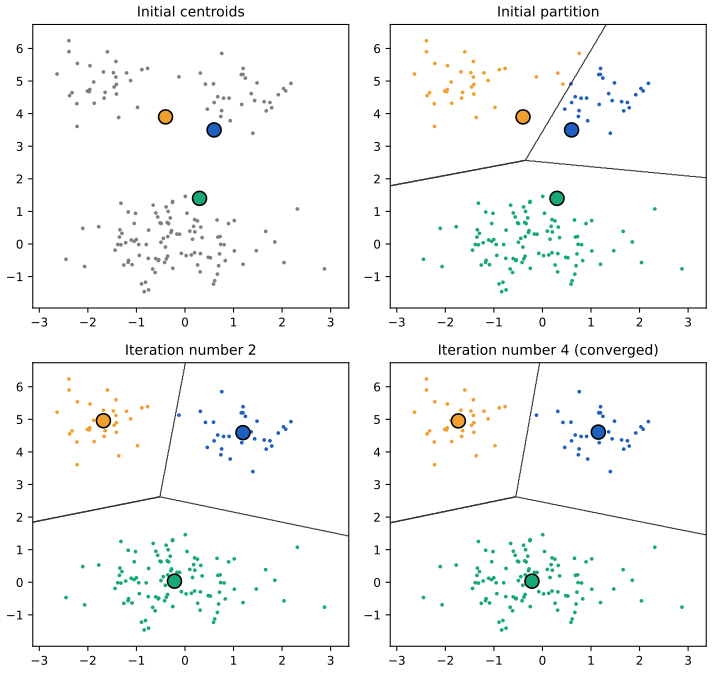
fig_14_6. Reproduces Hastie, Tibshirani and Friedman (2009), Figure 14.6. Download: PDF · SVG14.3.7 Gaussian Mixtures as Soft K-means Clustering
pp. 510–512 K-means is a limit of the EM algorithm (Section 8.5) for a mixture of \(K\) Gaussians with common covariance \(\sigma^2\bI\). The E-step gives each point a responsibility for each component, its relative density under that component, which here is a decreasing function of the distance to the component mean; the M-step recomputes the means as responsibility-weighted averages. So EM is a "soft" K-means, and as \(\sigma\to0\) the responsibilities become 0 or 1 and the two coincide.
See also (companion courses): Foundations of Deep Learning, Result 15.7 (K-means is the small-variance limit of EM, with rates); Bayesian and Probabilistic Machine Learning, Section 9.3.2.
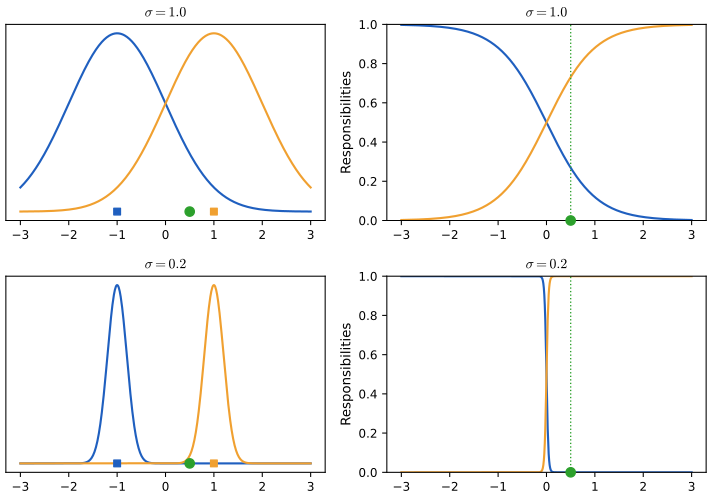
fig_14_7. Reproduces Hastie, Tibshirani and Friedman (2009), Figure 14.7. Download: PDF · SVGNote on the book: the responsibilities in Figure 14.7 are 0.27 and 0.73 p. 512
The caption gives 0.36 and 0.64 for \(\sigma=1\). With equal weights the responsibility of the component at \(+1\) for a point \(x\) is \(1/[1+e^{-2x/\sigma^2}]\) (the quadratic terms cancel, Result 14.7), which at \(x=0.5\), \(\sigma=1\) is \(1/(1+e^{-1})=0.731\). The book's values would need \(\sigma\approx1.7\) or the point at \(x\approx0.29\).
Result 14.7 (soft K-means and its hard limit; Exercise 14.2) pp. 510–511
For the mixture \(g(x)=\sum_k\pi_k\N(x;\mu_k,\sigma^2\bI)\) with \(\sigma\) known, EM iterates
\[ r_{ik}=\frac{\pi_k\exp(-\|x_i-\mu_k\|^2/2\sigma^2)}{\sum_l\pi_l\exp(-\|x_i-\mu_l\|^2/2\sigma^2)},\qquad \pi_k\leftarrow\frac1N\sum_ir_{ik},\qquad \mu_k\leftarrow\frac{\sum_ir_{ik}x_i}{\sum_ir_{ik}}. \]If no point is equidistant from two current means, then as \(\sigma\to0\) the responsibilities tend to \(r_{ik}=1\{k=\argmin_l\|x_i-\mu_l\|\}\) and the M-step for the means becomes step 1 of Algorithm 14.1: one EM iteration tends to one K-means iteration.
Proof
The derivation of the E- and M-steps is the solution to Exercise 14.2. For the limit, divide numerator and denominator by the term of the closest mean \(l^*\): \(r_{ik}=\pi_ke^{-\Delta_k/2\sigma^2}/\sum_l\pi_le^{-\Delta_l/2\sigma^2}\) with \(\Delta_l=\|x_i-\mu_l\|^2-\|x_i-\mu_{l^*}\|^2\ge0\), zero only for \(l=l^*\). As \(\sigma\to0\) each term with \(\Delta_l>0\) tends to 0 (the weights \(\pi_l>0\) are fixed), so \(r_{il^*}\to1\). Then \(\mu_k\) tends to the mean of the points assigned to \(k\). For two components on the line,
\[ \log(r_{i1}/r_{i0})=\log(\pi_1/\pi_0)+[(x-\mu_0)^2-(x-\mu_1)^2]/2\sigma^2, \]which for \(\mu_{0,1}=\mp1\) is \(2x/\sigma^2\): the curves in Figure 14.7 are logistic functions of slope \(2/\sigma^2\). On the data of Figure 14.4 from the start of Figure 14.6, EM with \(\sigma=0.1\) ends at exactly the K-means centres and partition. ∎
14.3.8 Example: Human Tumor Microarray Data
pp. 512–514 The microarray data of Chapter 1 are a \(6830\times64\) matrix: expression of 6830 genes (rows) in 64 cancer samples (columns). Here the 64 samples are clustered as vectors in \(\R^{6830}\), without using their labels. Figure 14.8 shows the within-cluster sum of squares for \(K=1,\dots,10\) (best of 300 random starts each); there is no clear kink.
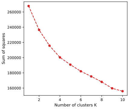
fig_14_8. Reproduces Hastie, Tibshirani and Friedman (2009), Figure 14.8. Download: PDF · SVGTable 14.2 cross-tabulates the three clusters (\(K=3\)) against the cancer types (the K562 and MCF7 cell-line repeats are counted with their types):
| Cluster | Breast | CNS | Colon | K562 | Leukemia | MCF7 | Melanoma | NSCLC | Ovarian | Prostate | Renal | Unknown |
|---|---|---|---|---|---|---|---|---|---|---|---|---|
| 1 | 3 | 5 | 0 | 0 | 0 | 0 | 1 | 7 | 6 | 2 | 9 | 1 |
| 2 | 2 | 0 | 7 | 2 | 6 | 2 | 0 | 2 | 0 | 0 | 0 | 0 |
| 3 | 2 | 0 | 0 | 0 | 0 | 0 | 7 | 0 | 0 | 0 | 0 | 0 |
Note on the book: Table 14.2 seems to have the Colon and Melanoma columns exchanged in clusters 2 and 3 p. 513
Our best K-means partition (criterion 215746, the lowest of 300 random starts) has clusters of sizes 34, 21 and 9, like the book's, and cluster 1 agrees with the book's first row in every column. Clusters 2 and 3 agree with the book's rows too, except that the seven colon samples and the seven melanoma samples change places: in the book cluster 2 holds the melanomas and cluster 3 the colons. The text supports our version: it says the two breast samples placed with the melanomas were later found to be metastatic melanomas, and in our partition the 9-sample cluster is exactly the seven melanomas plus two breast samples. The book's arrangement (melanomas with the leukemias, colons alone with two breast samples) also appears as a local optimum, but with a larger criterion.
K-means groups the samples of the same cancer well, but it gives no ordering within a cluster, and the clusters for different \(K\) need not be nested. Hierarchical clustering (Section 14.3.12) removes both drawbacks.
14.3.9 Vector Quantization
pp. 514–515 In image compression, K-means (called Lloyd's algorithm there) is vector quantisation. The image is cut into \(2\times2\) blocks of pixels, each a vector in \(\R^4\); K-means on the blocks gives a codebook of \(K\) centroids (codewords); each block is encoded by the index of its closest codeword and decoded by replacing it with that codeword. The photograph of R. A. Fisher used in the book is not available, so Figure 14.9 compresses a public-domain portrait of the computer scientist Grace Hopper (the central \(512\times512\) pixels of a photograph distributed with matplotlib).
See also (companion courses): Bayesian and Probabilistic Machine Learning, Filling the gap 9.4 (the compression arithmetic); Foundations of Deep Learning, Filling the gap 15.2 and the K-means quantisation demo.
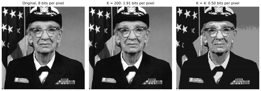
fig_14_9, vq_compress. Reproduces the method of Hastie, Tibshirani and Friedman (2009), Figure 14.9. Download: PDF · SVGFilling the gap 14.6: the rates, and why an entropy code does better p. 515
Derivation
A \(512\times512\) image has \(256^2\) blocks of four pixels. A fixed-length index for \(K\) codewords needs \(\log_2K\) bits per block, i.e. \(\log_2K/4\) bits per pixel, against 8 for the original: a storage fraction of \(\log_2K/32\) (0.239 for \(K=200\), 0.0625 for \(K=4\)). The codebook adds \(4K\) numbers, negligible next to \(256^2\) indices.
If codeword \(\ell\) is used by a fraction \(p_\ell\) of the blocks, Shannon's source coding theorem says that a prefix code can use on average as few as \(H=-\sum_\ell p_\ell\log_2p_\ell\) bits per block (and no fewer), and \(H\le\log_2K\) with equality only for equal frequencies (Jensen's inequality applied to the concave \(\log\)). Frequent codewords (large plain areas) get short codes. Per pixel the rate is \(H/4\): 1.72 and 0.42 bits for our two codebooks (the book reports 1.42 and 0.39 for its image). The book's distortions (0.89 and 16.95) are on a different scale from our mean squared errors in grey levels, so only the rates are comparable. ∎
14.3.10 K-medoids
pp. 515–518 Squared Euclidean distance requires quantitative variables and is sensitive to outliers. Only step 1 of K-means uses it, through (14.32); replacing the mean by an explicit minimisation over centres that are themselves observations allows any dissimilarity, even a proximity matrix with no attributes at all.
Algorithm 14.2 K-medoids clustering p. 516
- For the current assignment \(C\), find in each cluster the observation with the smallest total dissimilarity to the other members, \[ i_k^*=\argmin_{\{i:C(i)=k\}}\sum_{C(i')=k}D(x_i,x_{i'}), \tag{14.35} \] and set \(m_k=x_{i_k^*}\).
- For the current centres, assign each observation to the closest: \[ C(i)=\argmin_{1\le k\le K}D(x_i,m_k). \tag{14.36} \]
- Repeat until the assignments do not change.
Step 1 costs \(O(N_k^2)\) per cluster instead of \(O(N_k)\). With only indices \(i_1,\dots,i_K\) of the centres, the assignment step is
\[ C(i)=\argmin_{1\le k\le K}d_{ii_k}, \tag{14.37} \]and the alternation is a heuristic search for
\[ \min_{C,\{i_k\}_1^K}\sum_{k=1}^K\sum_{C(i)=k}d_{ii_k}. \tag{14.38} \]Result 14.8 (K-medoids descends on (14.38)) pp. 516–517
Each step of Algorithm 14.2 does not increase (14.38); with ties kept, it stops after finitely many iterations. The exchange search of Kaufman and Rousseeuw (1990) (swap a medoid with a non-medoid when that lowers (14.38)) also descends and stops, and can only improve on a fixed point of Algorithm 14.2.
Proof
For fixed \(C\), (14.38) is a sum over clusters of \(\sum_{C(i)=k}d_{ii_k}\), and (14.35) minimises each term over the allowed centres. For fixed centres, (14.38) is a sum over \(i\) of \(d_{ii_{C(i)}}\), minimised term by term by (14.37). The argument of Result 14.6 (strict decrease when the partition changes, finitely many partitions) applies verbatim. A swap is accepted only if it lowers the criterion with the optimal assignment for the new medoids, so the swap search is also a strict descent on a finite set of medoid sets; at a fixed point of the swap search no single swap helps, which includes the moves Algorithm 14.2 can make. ∎
See also (companion course): Statistical Methods for Modern Biology, Filling the gap 5.6 (medoids, PAM's BUILD and SWAP) and the k-means and PAM demo.
Example: country dissimilarities. Political science students rated the dissimilarity of 12 countries; Table 14.3 of the book gives the averages (Kaufman and Rousseeuw, 1990). Only dissimilarities are available, so K-means cannot be used. Running Algorithm 14.2 from all 220 sets of three starting medoids, the best fixed point has medoids USA, Zaire and Cuba and criterion 30.08; the swap search cannot improve it, and enumerating all 220 medoid triples confirms it is the global minimum of (14.38).
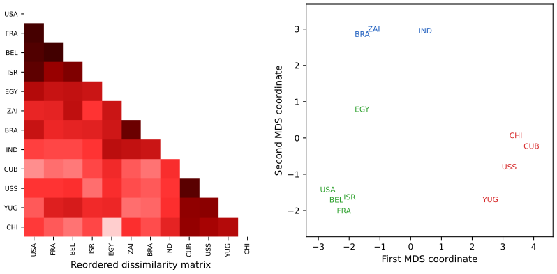
fig_14_10, kmedoids, pam_swap. Reproduces Hastie, Tibshirani and Friedman (2009), Figure 14.10. Download: PDF · SVG14.3.11 Practical Issues
pp. 518–520 Starting centres can be random or chosen forward stepwise (each new centre minimising (14.33) or (14.38) given the previous ones). When \(K\) is not dictated by the application, it is estimated from the within-cluster dissimilarities \(W_1,W_2,\dots,W_{K_{\max}}\). These always decrease with \(K\), even on independent test data, so cross-validation does not help. If there are \(K^*\) well-separated groups, splitting them apart gives large drops \(W_K-W_{K+1}\) for \(K\lt K^*\) and smaller ones after, and one looks for a kink. The gap statistic (Tibshirani et al., 2001b) compares \(\log W_K\) with its average over data drawn uniformly on a box containing the data, \(\mathrm{Gap}(K)\), with \(s'_K=s_K\sqrt{1+1/B}\) from \(B\) reference sets, and estimates
\[ K^*=\argmin_K\{K\given G(K)\ge G(K+1)-s'_{K+1}\}. \tag{14.39} \]Filling the gap 14.7: why \(W_K\) keeps falling, even on test data, and where \(\sqrt{1+1/B}\) comes from p. 519
Derivation
Training data. Let \(W_K^*\) be the global minimum of the K-means criterion. Take an optimal \(K\)-partition and split off one point that is not at its cluster mean as a new singleton cluster (possible whenever \(K\lt N\) and not all points of every cluster coincide). Removing a point \(x\) from a cluster of size \(n\) with mean \(\bar x\) lowers its sum of squares by \(\frac{n}{n-1}\|x-\bar x\|^2>0\), and the singleton costs nothing, so \(W^*_{K+1}\lt W^*_K\).
Test data. For new data the criterion is \(\sum_i\min_k\|x_i-m_k\|^2\) with the trained centres. Adding a centre can only lower each \(\min_k\), and as \(K\) grows the centres fill the support of the distribution, so the expected test criterion tends to 0. Unlike prediction error, there is no variance penalty for a richer description, so no U-shape for cross-validation to find.
The standard error. The reference curve is the average \(\bar\ell_K=\frac1B\sum_b\log W^{(b)}_K\) of \(B\) simulated values with sample standard deviation \(s_K\). \(\mathrm{Gap}(K)\) estimates \(\E\log W_K^{\rm ref}-\log W_K\); treating the observed \(\log W_K\) as one more draw with the reference spread, the variance of the difference is
\[ \Var(\bar\ell_K)+\Var(\log W_K)\approx s_K^2/B+s_K^2=s_K^2(1+1/B). \]The rule (14.39) takes the smallest \(K\) whose gap is within one such standard error of the next gap. See also Filling the gap 5.13 of the companion course. ∎
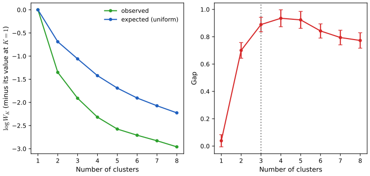
fig_14_11, gap_statistic. Reproduces Hastie, Tibshirani and Friedman (2009), Figure 14.11. Download: PDF · SVGSee also (companion course): Statistical Methods for Modern Biology, Section 5.7.1 (using the gap statistic) and the choosing-k demo.
14.3.12 Hierarchical Clustering
pp. 520–528 Hierarchical methods need no \(K\) and no start; they need a dissimilarity between groups. Agglomerative (bottom-up) methods start from \(N\) singletons and merge the two closest groups at each of \(N-1\) steps; divisive (top-down) methods split one group into two at each step. The result is a rooted binary tree, drawn as a dendrogram with each merge at the height of the dissimilarity between the merged groups. Cutting it at a height gives a partition, and partitions at different heights are nested.
See also (companion course): Statistical Methods for Modern Biology, Section 5.6, Filling the gaps 5.9 (the Lance–Williams recursion) and 5.10, and the hierarchical clustering demo.
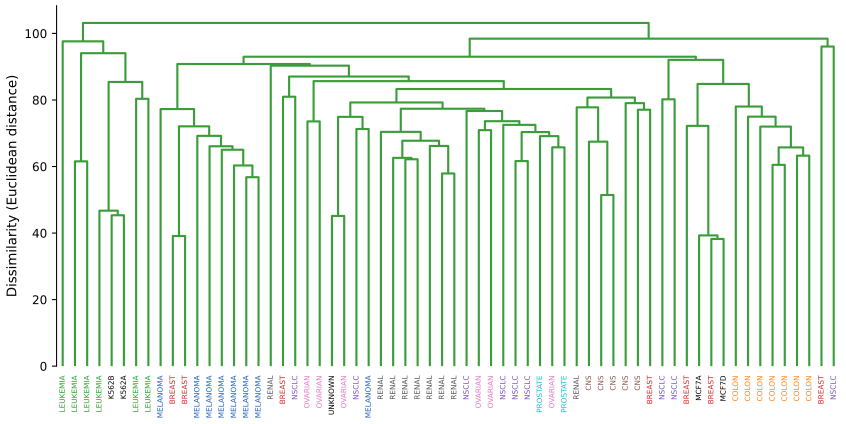
fig_14_12, agglomerate. Reproduces Hastie, Tibshirani and Friedman (2009), Figure 14.12. Download: PDF · SVGHierarchical methods impose a hierarchy whether or not the data have one. The cophenetic dissimilarity \(C_{ii'}\) is the height at which \(i\) and \(i'\) first join; the correlation between the \(N(N-1)/2\) values \(d_{ii'}\) and \(C_{ii'}\) (the cophenetic correlation) measures how well the tree represents the dissimilarities. Only \(N-1\) of the \(C_{ii'}\) can be distinct, and they satisfy the ultrametric inequality
\[ C_{ii'}\le\max\{C_{ik},C_{i'k}\} \tag{14.40} \]for any three observations.
Result 14.9 (dendrograms are ultrametrics; ultrametric triangles are isosceles) pp. 522–523, (14.40)
(a) If the merge heights of a hierarchical clustering are non-decreasing, the cophenetic dissimilarities satisfy (14.40). (b) For any three points of an ultrametric, the two largest of the three dissimilarities are equal. So Euclidean points whose distances form an ultrametric make only isosceles triangles whose third side is no longer than the two equal ones, which few real data sets satisfy.
Proof
(a) Let \(h=\max\{C_{ik},C_{i'k}\}\). At height \(h\) (after all merges at heights \(\le h\)), \(i\) is in the same group as \(k\), and \(i'\) is in the same group as \(k\), because groups only grow as the height increases. So \(i\) and \(i'\) are in one group at height \(h\), and they first joined at a height \(C_{ii'}\le h\).
(b) Label the three values \(a\le b\le c\). Applying (14.40) with the pair whose dissimilarity is \(c\) gives \(c\le\max\{a,b\}=b\), so \(b=c\). ∎
For the 64 samples the cophenetic correlation is 0.77 for average linkage, 0.66 for complete linkage and 0.68 for single linkage: average linkage represents the distances best, as it usually does.
Agglomerative clustering. The dissimilarity \(d(G,H)\) between groups is built from the \(d_{ii'}\) with \(i\in G\), \(i'\in H\). Single linkage (nearest neighbour) uses the closest pair,
\[ d_{SL}(G,H)=\min_{i\in G,\ i'\in H}d_{ii'}, \tag{14.41} \]complete linkage (furthest neighbour) the furthest pair,
\[ d_{CL}(G,H)=\max_{i\in G,\ i'\in H}d_{ii'}, \tag{14.42} \]and group average linkage the average,
\[ d_{GA}(G,H)=\frac1{N_GN_H}\sum_{i\in G}\sum_{i'\in H}d_{ii'}. \tag{14.43} \]Result 14.10 (the merge heights never decrease for these three linkages) p. 521
For (14.41)–(14.43) the dissimilarity at which merges happen is non-decreasing along the agglomeration, so the dendrogram can be drawn with heights equal to the merge dissimilarities and (by Result 14.9) the cophenetic dissimilarities form an ultrametric.
Proof
When \(G\) and \(H\) are merged into \(G\cup H\), the new dissimilarity to any other group \(K\) is \(\min\{d(G,K),d(H,K)\}\) (single), \(\max\{\dots\}\) (complete), or \(\frac{N_G}{N_G+N_H}d(G,K)+\frac{N_H}{N_G+N_H}d(H,K)\) (average): the Lance–Williams updates, which follow from (14.41)–(14.43) by splitting the min, max or sum over \(G\cup H\) into its parts. In all three cases the new value is at least \(\min\{d(G,K),d(H,K)\}\). The merged pair was the closest, so \(d(G,K)\ge d(G,H)\) and \(d(H,K)\ge d(G,H)\), hence \(d(G\cup H,K)\ge d(G,H)\): no future merge can be cheaper than the current one, and dissimilarities between untouched groups do not change. By induction the merge heights are non-decreasing. (Centroid linkage, which is not of this form, can produce inversions; see Filling the gap 5.10 of the companion course.) ∎
If the clusters are compact and well separated, the three linkages agree. Otherwise single linkage chains: one small dissimilarity suffices to join two groups, so it can produce clusters of large diameter
\[ D_G=\max_{i\in G,\ i'\in G}d_{ii'}, \tag{14.44} \]while complete linkage produces compact clusters whose members may be closer to other clusters than to some of their own. Group average is a compromise, but unlike the other two it is not invariant under monotone transformations of the \(d_{ii'}\).
Filling the gap 14.8: invariance, and what the three linkages estimate p. 525, (14.45)
Derivation
Invariance. If \(h\) is strictly increasing, \(\min_{i,i'}h(d_{ii'})=h(\min d_{ii'})\) and likewise for the max, so every comparison made by single or complete linkage gives the same answer after transforming: the same merges in the same order, with heights transformed by \(h\). An average does not commute with \(h\) unless \(h\) is affine, so group-average merges can change.
Population limits. Suppose cluster \(G\) is a sample of size \(N_G\) from a density \(p_G\) and \(H\) from \(p_H\). By the law of large numbers \(d_{GA}(G,H)\) tends to
\[ \int\int d(x,x')\,p_G(x)\,p_H(x')\,dx\,dx', \tag{14.45} \]a property of the two populations. If the supports of \(p_G\) and \(p_H\) touch (for example two overlapping Gaussians), the minimum of \(N_GN_H\) distances tends to the distance between the supports, which is 0; if the supports are unbounded, the maximum tends to \(\infty\). So \(d_{SL}\to0\) and \(d_{CL}\to\infty\) for overlapping Gaussian clusters, whatever their separation: neither estimates a population quantity that depends on the densities beyond their supports. ∎
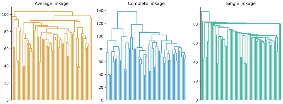
fig_14_13. Reproduces Hastie, Tibshirani and Friedman (2009), Figure 14.13. Download: PDF · SVGOrdering the leaves. Each merge can be drawn with either subtree on the left, so a leaf order needs a rule. Following the book, the tighter subtree (smaller merge height) goes first, and two single leaves keep their index order. Applying average linkage separately to the genes and to the samples and ordering both by this rule gives the two-way display of Figure 14.14, far more readable than the random order of Figure 1.3.
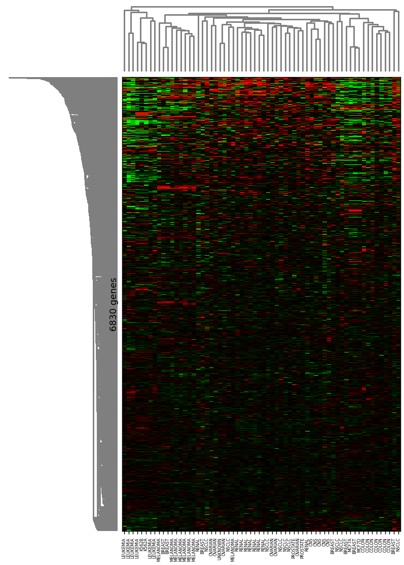
fig_14_14, tight_first_linkage. Reproduces Hastie, Tibshirani and Friedman (2009), Figure 14.14. Download: PDF · PNGDivisive clustering could apply K-means or K-medoids with \(K=2\) recursively, but the result depends on the starts and need not have monotone heights. The method of Macnaughton-Smith et al. (1965) avoids this. Start a new group \(H\) with the observation of \(G\) whose average dissimilarity to the others is largest. Then, for each \(i\) still in \(G\), compute
\[ \delta_i=\big(\text{average of } d_{ii'} \text{ over the other } i'\in G\big)-\big(\text{average of } d_{ii'} \text{ over } i'\in H\big), \]move the observation with the largest \(\delta_i\) to \(H\), and repeat while the largest \(\delta_i\) is positive, i.e. while some member of \(G\) is on average closer to \(H\) than to the rest of \(G\). (The book phrases the difference the other way round, "average distance from those in H, minus that for the remaining observations in G", but its stopping rule, "no longer any observations in G that are, on average, closer to those in H", requires \(\delta_i\) as written here.) The splitting continues recursively on the cluster of largest diameter (14.44) or largest average dissimilarity
\[ \bar d_G=\frac1{N_G^2}\sum_{i\in G}\sum_{i'\in G}d_{ii'}, \]until all clusters are singletons or have zero internal dissimilarity.
14.4 Self-Organizing Maps
pp. 528–534 The self-organising map (SOM; Kohonen, 1990) is a constrained K-means: the \(K=q_1q_2\) prototypes \(m_j\in\R^p\) are attached to the nodes \(\ell_j\in\{1,\dots,q_1\}\times\{1,\dots,q_2\}\) of a grid, and neighbouring nodes are encouraged to have nearby prototypes, so that the prototypes form a bent two-dimensional sheet in \(\R^p\) onto which the data can be mapped. Start with the prototypes on a regular grid in the plane of the first two principal components ("buttons sewn on the plane"). Then process the observations one at a time: for \(x_i\), find the closest prototype \(m_j\) and move every prototype \(m_k\) whose node is a neighbour of \(\ell_j\) (\(\|\ell_j-\ell_k\|\le r\), which includes \(j\) itself) towards \(x_i\):
\[ m_k\leftarrow m_k+\alpha(x_i-m_k). \tag{14.46} \]The learning rate \(\alpha\) decreases from about 1 to 0 and the radius \(r\) from \(R\) to 1 over a few thousand updates. A smoother version weights the move by a decreasing function \(h\) of the grid distance:
\[ m_k\leftarrow m_k+\alpha h(\|\ell_j-\ell_k\|)(x_i-m_k). \tag{14.47} \]The batch version replaces each prototype by a weighted average,
\[ m_j=\frac{\sum w_kx_k}{\sum w_k}, \tag{14.48} \]over the points \(x_k\) whose closest prototype is a grid neighbour of \(m_j\), with weights \(w_k\) equal to 1 (rectangular) or decreasing with the grid distance.
Result 14.11 (with the smallest neighbourhood, the SOM is K-means) pp. 529–531
(a) If \(r\lt1\), so each neighbourhood is the winning node alone, the online update (14.46) with \(\alpha=1/n_j\) (\(n_j\) the number of points node \(j\) has won so far, counting the start as one) keeps every prototype equal to the running mean of the points it has won: MacQueen's online K-means. With a slowly decreasing \(\alpha\) it is a stochastic approximation of K-means.
(b) With rectangular weights and \(r\lt1\), one batch update (14.48) is exactly one iteration of Algorithm 14.1 (assignment to the closest prototype, then means).
Proof
(a) Only the winner moves. If \(m_j\) is the mean of \(n-1\) points and \(x\) is the \(n\)-th point it wins, \(m_j+\frac1n(x-m_j)=\frac{(n-1)m_j+x}{n}\) is the mean of the \(n\) points. In general (14.46) with only the winner moving is a Robbins–Monro step for the stationarity condition \(\E[(X-m_j)1\{X\in V_j\}]=0\) of the K-means criterion, where \(V_j\) is the Voronoi cell of \(m_j\) (see Filling the gap 9.2 of the companion course).
(b) With rectangular weights and only the node itself in its neighbourhood, (14.48) averages the points whose closest prototype is \(m_j\): that is (14.34) followed by (14.32). ∎
Example: the half-sphere data. Ninety points in three clusters of 30 lie near the unit sphere, around \((0,0,1)\) (red, the tightest), \((1,0,0)\) and \((0,1,0)\) (Exercise 14.5 gives the recipe). A \(5\times5\) SOM with \(R=2\) (about a third of the prototypes in each neighbourhood at the start) is run for 40 passes over the data, 3600 updates, with \(\alpha\) and \(r\) decreasing linearly.
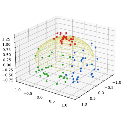
fig_14_15, half_sphere. Reproduces Hastie, Tibshirani and Friedman (2009), Figure 14.15. Download: PDF · SVG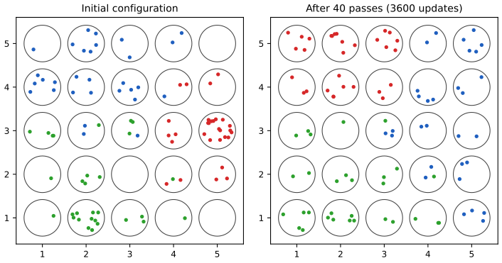
fig_14_16, som_online. Reproduces Hastie, Tibshirani and Friedman (2009), Figure 14.16. Download: PDF · SVG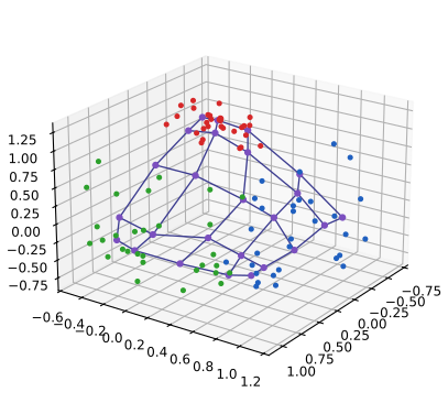
fig_14_17. Reproduces Hastie, Tibshirani and Friedman (2009), Figure 14.17. Download: PDF · SVG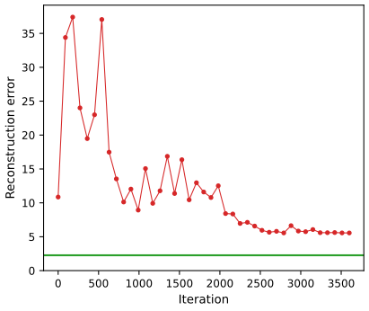
fig_14_18. Reproduces Hastie, Tibshirani and Friedman (2009), Figure 14.18. Download: PDF · SVGNote on the book: the noise level of the half-sphere data pp. 529–532 and Exercise 14.5
Exercise 14.5 adds Gaussian noise of standard deviation 0.6 to each coordinate. With that noise the clusters are not "near the surface of a half sphere": K-means with 25 centres leaves a reconstruction error of about 15 and the SOM about 34, while the total sum of squares is 186; Figure 14.18 shows a K-means error near 2.5 and a final SOM error near 8. With standard deviation 0.1 we get 2.27 and 5.6, in line with the figure, so the figures were presumably made with a much smaller noise level than the exercise states (or 0.6 is a typo). We use 0.1. Also, the text places the red cluster at \((0,1,0)\), but in the exercise the tight cluster (polar angle within \(\pi/8\) of 0) is the one at \((0,0,1)\), as Figure 14.15 shows.
Document organisation. The book's Figure 14.19 shows a WEBSOM map of 12,088 newsgroup articles (Kohonen et al., 2000), built on term-frequency vectors reduced by a random projection; the corpus and map are not available, so the figure is not reproduced. The idea is a SOM on document vectors, with each node labelled by its typical words and a "zoom" down to the articles.
14.5 Principal Components, Curves and Surfaces
p. 534 Principal components were met in Section 3.5.1 as the directions behind ridge regression and principal components regression. Here they are the best linear approximations of the data of each rank \(q\); Sections 14.5.2–14.5.5 and 14.9 make them nonlinear, sparse or local.
14.5.1 Principal Components
pp. 534–541 The rank-\(q\) linear model for \(x_1,\dots,x_N\in\R^p\) is
\[ f(\lambda)=\mu+\bV_q\lambda, \tag{14.49} \]with \(\mu\in\R^p\), \(\bV_q\) a \(p\times q\) matrix with orthonormal columns and \(\lambda\in\R^q\): an affine subspace of dimension \(q\). Fitting it by least squares means minimising the reconstruction error
\[ \min_{\mu,\{\lambda_i\},\bV_q}\sum_{i=1}^N\|x_i-\mu-\bV_q\lambda_i\|^2. \tag{14.50} \]Optimising over \(\mu\) and the \(\lambda_i\) gives
\[ \hat\mu=\bar x, \tag{14.51} \] \[ \hat\lambda_i=\bV_q^\T(x_i-\bar x), \tag{14.52} \]which leaves
\[ \min_{\bV_q}\sum_{i=1}^N\|(x_i-\bar x)-\bV_q\bV_q^\T(x_i-\bar x)\|^2. \tag{14.53} \]Result 14.12 (partial optimisation of (14.50); Exercise 14.7) p. 535
For fixed \(\bV_q\), (14.51)–(14.52) attain the minimum of (14.50) over \(\mu\) and \(\{\lambda_i\}\), so (14.50) reduces to (14.53). The minimising \(\mu\) is not unique: the minimisers are exactly \(\mu=\bar x+\bV_qc\), \(c\in\R^q\), with \(\lambda_i=\bV_q^\T(x_i-\bar x)-c\); all give the same fitted values.
Proof
For fixed \(\mu\) and \(\bV_q\), each \(\lambda_i\) is a least-squares coefficient of \(x_i-\mu\) on the orthonormal columns of \(\bV_q\): \(\lambda_i=\bV_q^\T(x_i-\mu)\), and the residual is \((\bI-\bH_q)(x_i-\mu)\) with \(\bH_q=\bV_q\bV_q^\T\) the orthogonal projection onto the column space. The criterion becomes \(\sum_i\|(\bI-\bH_q)(x_i-\mu)\|^2\). Write \(\bP=\bI-\bH_q\), also an orthogonal projection, and decompose as in Result 14.6:
\[ \sum_i\|\bP(x_i-\mu)\|^2=\sum_i\|\bP(x_i-\bar x)\|^2+N\|\bP(\bar x-\mu)\|^2. \]The minimum over \(\mu\) is attained exactly when \(\bP(\bar x-\mu)=0\), i.e. \(\mu-\bar x\in\span(\bV_q)\), \(\mu=\bar x+\bV_qc\). Then \(\lambda_i=\bV_q^\T(x_i-\bar x)-c\) (using \(\bV_q^\T\bV_q=\bI\)), and the fitted value \(\mu+\bV_q\lambda_i=\bar x+\bH_q(x_i-\bar x)\) does not depend on \(c\). Taking \(c=0\) gives (14.51)–(14.52), and substituting gives (14.53). ∎
Assume from now on that the data are centred (\(\bar x=0\)) and stacked in the rows of the \(N\times p\) matrix \(\bX\), with singular value decomposition
\[ \bX=\bU\bD\bV^\T, \tag{14.54} \]\(\bU\) (\(N\times p\)) and \(\bV\) (\(p\times p\)) with orthonormal columns and \(\bD=\diag(d_1\ge\dots\ge d_p\ge0)\). The solution of (14.53) is \(\bV_q\) = the first \(q\) columns of \(\bV\); the optimal \(\hat\lambda_i\) are the rows of \(\bU_q\bD_q\), the first \(q\) principal components (columns of \(\bU\bD\)), and \(\bH_q=\bV_q\bV_q^\T\) maps each \(x_i\) to its rank-\(q\) reconstruction.
See also (companion courses): Bayesian and Probabilistic Machine Learning, Result 12.3 (minimum-error PCA); Foundations of Deep Learning, Result 16.2; Statistical Methods for Modern Biology, Theorem 7.4 (Eckart–Young–Mirsky).
Result 14.13 (the best rank-\(q\) subspace, and the Eckart–Young theorem) pp. 535–536
(a) Over all \(p\times q\) \(\bV_q\) with \(\bV_q^\T\bV_q=\bI\), (14.53) equals \(\|\bX\|_F^2-\Tr(\bV_q^\T\bX^\T\bX\bV_q)\) and is minimised by the first \(q\) right singular vectors, with minimum \(\sum_{j>q}d_j^2\); the minimiser is unique (up to a rotation within the span) when \(d_q>d_{q+1}\).
(b) Equivalently, \(\bX_q=\bU_q\bD_q\bV_q^\T=\bX\bV_q\bV_q^\T\) is a closest matrix of rank at most \(q\) to \(\bX\) in Frobenius norm (Eckart and Young, 1936).
(c) \(\bX v_1\) has the largest sample variance among all \(\bX v\) with \(\|v\|=1\); \(\bX v_2\) the largest among those with \(v\perp v_1\); and so on.
Proof
(a) Since \(\bH_q\) is an orthogonal projection, \(\|x_i-\bH_qx_i\|^2=\|x_i\|^2-\|\bV_q^\T x_i\|^2\), and summing, (14.53)
\[ =\|\bX\|_F^2-\|\bX\bV_q\|_F^2=\|\bX\|_F^2-\Tr(\bV_q^\T\bS\bV_q) \]with \(\bS=\bX^\T\bX=\bV\bD^2\bV^\T\). Write \(\bV_q=\bV\bA\) with \(\bA=\bV^\T\bV_q\), also with orthonormal columns. Then \(\Tr(\bV_q^\T\bS\bV_q)=\sum_jd_j^2a_j\), where \(a_j=\sum_k A_{jk}^2\) is the squared norm of row \(j\) of \(\bA\). The weights satisfy \(0\le a_j\le1\) (row norms of a matrix with orthonormal columns, completed to an orthogonal matrix, are at most 1) and \(\sum_ja_j=\|\bA\|_F^2=q\). A linear function \(\sum_jd_j^2a_j\) with \(d_1^2\ge d_2^2\ge\cdots\) over this set is maximised by putting \(a_1=\dots=a_q=1\) and the rest 0 (move weight from any \(j>q\) to any \(j\le q\) with \(a_j\lt1\) without decreasing the sum), with value \(\sum_{j\le q}d_j^2\). The choice \(\bV_q=\) first \(q\) columns of \(\bV\) attains it. If \(d_q>d_{q+1}\), any weight on \(j>q\) strictly lowers the sum, so the maximiser has \(a_j=0\) for \(j>q\): its columns lie in \(\span(v_1,\dots,v_q)\).
(b) For a matrix \(\bY\) of rank at most \(q\), its row space lies in some \(q\)-dimensional subspace with orthonormal basis \(\bV_q\); then \(\|\bX-\bY\|_F^2\ge\|\bX-\bX\bV_q\bV_q^\T\|_F^2\) (projecting each row of \(\bX\) onto that subspace is the best approximation row by row), which by (a) is at least \(\sum_{j>q}d_j^2=\|\bX-\bX_q\|_F^2\). A complete proof with the spectral norm as well is in Filling the gap 7.9 of the companion course.
(c) With centred columns the sample variance of \(\bX v\) is \(v^\T\bS v/N\). This is (a) with \(q=1\): \(v^\T\bS v\le d_1^2\) with equality at \(v_1\). Restricted to \(v\perp v_1,\dots,v_{k-1}\), write \(v=\sum_{j\ge k}c_jv_j\), \(\sum c_j^2=1\): \(v^\T\bS v=\sum_{j\ge k}d_j^2c_j^2\le d_k^2\), attained at \(v_k\). ∎
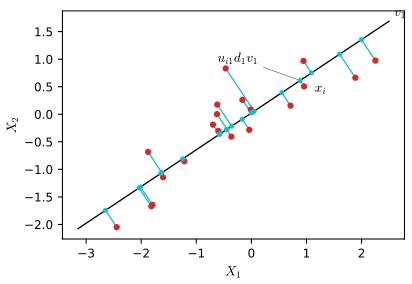
fig_14_20. Reproduces Hastie, Tibshirani and Friedman (2009), Figure 14.20. Download: PDF · SVG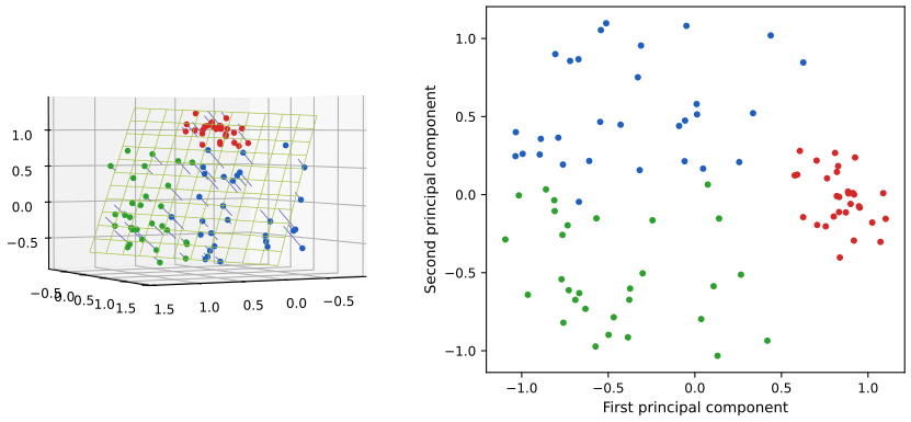
fig_14_21. Reproduces Hastie, Tibshirani and Friedman (2009), Figure 14.21. Download: PDF · SVGExample: handwritten digits. The 658 threes of the zip-code training set (Chapter 1) are points in \(\R^{256}\) (\(16\times16\) grey levels). Figure 14.22 shows a sample; writing styles vary in thickness, slant and the length of the lower tail.
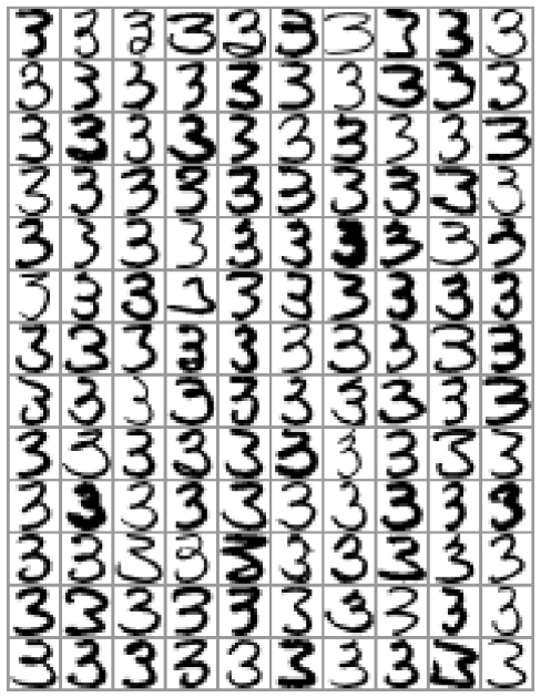
fig_14_22. Reproduces Hastie, Tibshirani and Friedman (2009), Figure 14.22. Download: PDF · SVG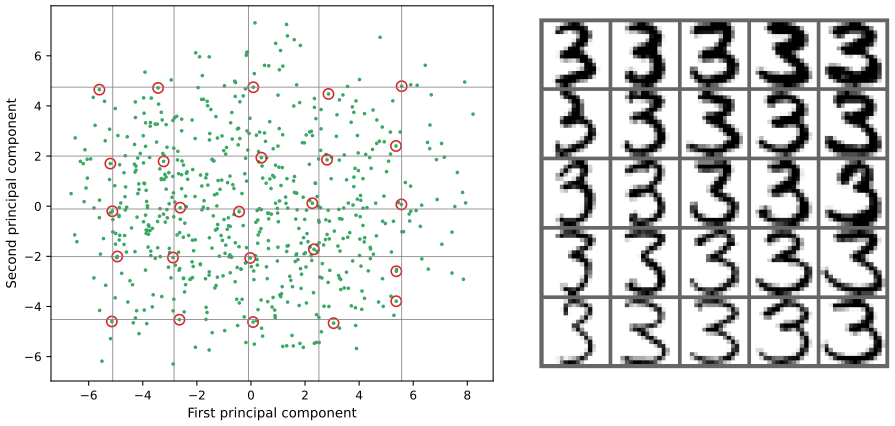
fig_14_23. Reproduces Hastie, Tibshirani and Friedman (2009), Figure 14.23. Download: PDF · SVGIn terms of (14.49) the rank-two model is
\[ \hat f(\lambda)=\bar x+\lambda_1v_1+\lambda_2v_2, \tag{14.55} \]with the mean and the two directions shown as images below. Twelve components explain 63.4% of the variance and 52 are needed for 90% (the book: 63% and about 50).
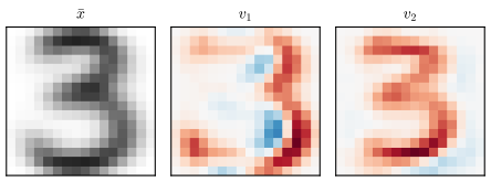
fig_14_23b. Download: PDF · SVG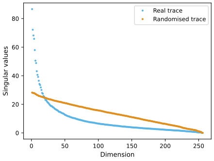
fig_14_24. Reproduces Hastie, Tibshirani and Friedman (2009), Figure 14.24. Download: PDF · SVGFilling the gap 14.9: what the randomised trace shows p. 537
Derivation
Permuting each column independently keeps the column variances, so the sum of squared singular values (the total variance times \(N\)) is the same for both traces: \(\sum_jd_j^2=\|\bX\|_F^2\). After permutation the columns are (nearly) uncorrelated, so \(\bX^\T\bX\) is close to the diagonal matrix of column sums of squares, and its eigenvalues spread the total over all 256 directions roughly as the sorted pixel variances (plus sampling noise): a slowly decreasing trace. In the real data the same total is concentrated in the leading directions, so the real trace must start above and end below the randomised one: the crossing point (here near dimension 20) is a rough guide to how many components carry structure beyond what independent pixels would give. ∎
Example: Procrustes transformations and shape averaging. Figure 14.25 shows two handwritten S's, each recorded as \(N=96\) corresponding points (landmarks) in \(\R^2\), the \(N\times2\) matrices \(\bX_1\) and \(\bX_2\) (the correspondence was obtained by time-warping the speed signal along each signature). A Procrustes transformation translates and rotates one set of points to match the other as closely as possible:
\[ \min_{\mu,\bR}\|\bX_2-(\bX_1\bR+\bone\mu^\T)\|_F, \tag{14.56} \]with \(\bR\) a \(p\times p\) orthogonal matrix (rotations and reflections), \(\mu\in\R^p\), and \(\|\bX\|_F^2=\Tr(\bX^\T\bX)\). Let \(\bar x_1,\bar x_2\) be the column means, \(\tilde\bX_1,\tilde\bX_2\) the centred matrices, and \(\tilde\bX_1^\T\tilde\bX_2=\bU\bD\bV^\T\). Then (Exercise 14.8)
\[ \hat\bR=\bU\bV^\T,\qquad \hat\mu=\bar x_2-\hat\bR^\T\bar x_1, \tag{14.57} \]and the minimum is the Procrustes distance. With a scale factor as well,
\[ \min_{\beta,\bR}\|\bX_2-\beta\bX_1\bR\|_F \tag{14.58} \](centred matrices), the rotation is the same and \(\hat\beta=\Tr(\bD)/\|\bX_1\|_F^2\).
Result 14.14 (the Procrustes solutions; Exercise 14.8) p. 540, (14.57)–(14.58)
(14.57) solves (14.56), and with scaling \(\hat\beta=\Tr(\bD)/\|\tilde\bX_1\|_F^2\). The Procrustes distance is \(\big(\|\tilde\bX_1\|_F^2+\|\tilde\bX_2\|_F^2-2\Tr(\bD)\big)^{1/2}\), and with scaling \(\big(\|\tilde\bX_2\|_F^2-\Tr(\bD)^2/\|\tilde\bX_1\|_F^2\big)^{1/2}\).
Proof
Location. For fixed \(\bR\), (14.56) is \(\sum_i\|x_{2i}-\bR^\T x_{1i}-\mu\|^2\) (rows written as column vectors), a least-squares problem for a common shift, minimised by the mean of the residuals: \(\mu=\bar x_2-\bR^\T\bar x_1\). Substituting, the criterion becomes \(\|\tilde\bX_2-\tilde\bX_1\bR\|_F^2\) with the centred matrices.
Rotation.
\[ \|\tilde\bX_2-\tilde\bX_1\bR\|_F^2=\|\tilde\bX_2\|_F^2+\|\tilde\bX_1\bR\|_F^2-2\Tr(\bR^\T\tilde\bX_1^\T\tilde\bX_2), \]and \(\|\tilde\bX_1\bR\|_F=\|\tilde\bX_1\|_F\) for orthogonal \(\bR\). So we must maximise
\[ \Tr(\bR^\T\bU\bD\bV^\T)=\Tr(\bV^\T\bR^\T\bU\bD)=\Tr(\bQ\bD)=\sum_jQ_{jj}d_j, \]where \(\bQ=\bV^\T\bR^\T\bU\) is orthogonal, so \(|Q_{jj}|\le1\). Since \(d_j\ge0\), the maximum is \(\sum_jd_j=\Tr(\bD)\), attained at \(\bQ=\bI\), i.e. \(\bR=\bU\bV^\T\). (If all \(d_j>0\) this maximiser is unique.)
Scale. For fixed \(\bR\),
\[ \|\tilde\bX_2-\beta\tilde\bX_1\bR\|_F^2=\|\tilde\bX_2\|^2-2\beta\Tr(\bR^\T\tilde\bX_1^\T\tilde\bX_2)+\beta^2\|\tilde\bX_1\|^2. \]For any \(\beta>0\) the best \(\bR\) is the same \(\bU\bV^\T\) (the \(\beta\) term only multiplies the trace), and then the quadratic in \(\beta\) is minimised at \(\beta=\Tr(\bD)/\|\tilde\bX_1\|_F^2\). Substituting gives the two distances. ∎
Note on the book: the location in (14.57) needs \(\hat\bR^\T\) p. 540
The book gives \(\hat\mu=\bar x_2-\hat\bR\bar x_1\). In (14.56) row \(i\) of \(\bX_1\bR+\bone\mu^\T\) is \(x_{1i}^\T\bR+\mu^\T\), i.e. the column vector \(\bR^\T x_{1i}+\mu\), so matching the means requires \(\hat\mu=\bar x_2-\hat\bR^\T\bar x_1\) (as stated above). The two agree only when \(\hat\bR\) is symmetric; for the two S's of Figure 14.25 the book's formula shifts the fitted shape by 246 units and raises the distance from 823 to 2549.
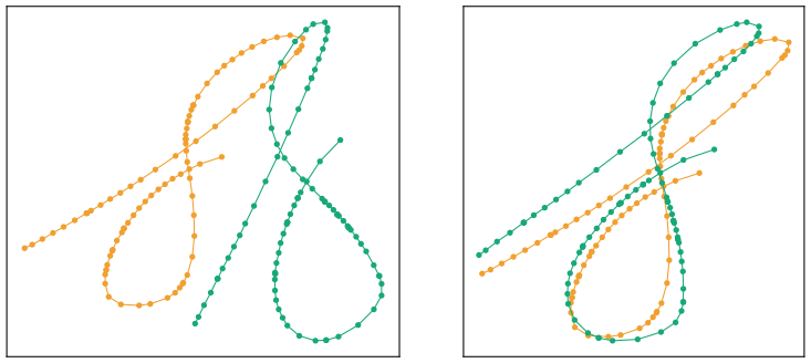
fig_14_25, procrustes. Reproduces Hastie, Tibshirani and Friedman (2009), Figure 14.25. Download: PDF · SVGThe Procrustes average of \(L\) shapes solves
\[ \min_{\{\bR_\ell\}_1^L,\bM}\sum_{\ell=1}^L\|\bX_\ell\bR_\ell-\bM\|_F^2, \tag{14.59} \]by alternation: start with \(\bM=\bX_1\); (1) solve the \(L\) Procrustes problems with \(\bM\) fixed, giving \(\bX'_\ell=\bX_\ell\hat\bR_\ell\); (2) set \(\bM=\frac1L\sum_\ell\bX'_\ell\); repeat. Each step minimises (14.59) over one block of variables, so the criterion never increases (it converges in 10 iterations for the three S's). The solution is determined only up to a common rotation of \(\bM\) and all \(\bR_\ell\).
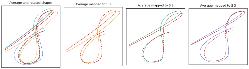
fig_14_26, procrustes_average. Reproduces Hastie, Tibshirani and Friedman (2009), Figure 14.26. Download: PDF · SVGMost generally, the affine-invariant average allows any non-singular \(p\times p\) matrices \(\bA_\ell\):
\[ \min_{\{\bA_\ell\}_1^L,\bM}\sum_{\ell=1}^L\|\bX_\ell\bA_\ell-\bM\|_F^2, \tag{14.60} \]with a normalisation such as \(\bM^\T\bM=\bI\) to rule out \(\bM=0\). It has a closed-form solution: with \(\bH_\ell=\bX_\ell(\bX_\ell^\T\bX_\ell)^{-1}\bX_\ell^\T\) the projection onto the column space of \(\bX_\ell\), \(\bM\) consists of the \(p\) leading eigenvectors of \(\bar\bH=\frac1L\sum_\ell\bH_\ell\).
Result 14.15 (the affine-invariant average; Exercise 14.10) p. 541, (14.60)
Subject to \(\bM^\T\bM=\bI_p\), (14.60) is minimised by \(\bM\) = the eigenvectors of the \(p\) largest eigenvalues of \(\bar\bH\), and \(\hat\bA_\ell=(\bX_\ell^\T\bX_\ell)^{-1}\bX_\ell^\T\bM\). The minimum is \(L\big(p-\sum_{j\le p}\gamma_j\big)\) with \(\gamma_j\) the eigenvalues of \(\bar\bH\).
Proof
For fixed \(\bM\), each \(\bA_\ell\) solves a multivariate least-squares problem (regress the columns of \(\bM\) on \(\bX_\ell\)), giving \(\hat\bA_\ell\) as stated and residual \(\|(\bI-\bH_\ell)\bM\|_F^2=\Tr(\bM^\T\bM)-\Tr(\bM^\T\bH_\ell\bM)\) (\(\bI-\bH_\ell\) is a projection). With \(\bM^\T\bM=\bI_p\) the sum over \(\ell\) is \(Lp-L\,\Tr(\bM^\T\bar\bH\bM)\). Maximising \(\Tr(\bM^\T\bar\bH\bM)\) over \(\bM\) with orthonormal columns is the problem of Result 14.13(a) with \(\bar\bH\) in place of \(\bS\) (Ky Fan's theorem): the leading \(p\) eigenvectors, with value \(\sum_{j\le p}\gamma_j\). The \(\hat\bA_\ell\) are non-singular in general (they would be singular only if some combination of the columns of \(\bM\) were orthogonal to the column space of \(\bX_\ell\)). ∎
For the three S's (centred), \(\bar\bH\) has leading eigenvalues 0.971, 0.898 and then 0.098: the three column spaces nearly share a two-dimensional subspace, and the residual (14.60) is \(3(2-0.971-0.898)=0.393\).
14.5.2 Principal Curves and Surfaces
pp. 541–544 A principal curve is a smooth one-dimensional curve \(f(\lambda)=[f_1(\lambda),\dots,f_p(\lambda)]\) in \(\R^p\) that passes through the "middle" of the data. For each \(x\), let \(\lambda_f(x)\) be the parameter of the point of the curve closest to \(x\). Then \(f\) is a principal curve of the distribution of \(X\) if
\[ f(\lambda)=\E\big(X\given\lambda_f(X)=\lambda\big): \tag{14.61} \]every point of the curve is the average of the points that project onto it (self-consistency). A distribution has many principal curves (Duchamp and Stuetzle, 1996); the smooth ones are of interest.
Principal points are the discrete analogue: \(k\) points minimising \(\E\min_j\|X-c_j\|^2\). Each is the mean of \(X\) over its Voronoi region, so they are the population version of K-means centroids, and a principal curve is like infinitely many principal points constrained to lie on a smooth curve, as an SOM constrains K-means centres to a sheet.
Filling the gap 14.10: the two principal points of a circular normal distribution p. 542
Derivation
Let \(X\sim\N(0,\sigma^2\bI_p)\). For one point the best choice is the mean, since \(\E\|X-c\|^2=p\sigma^2+\|c\|^2\). For two points \(c_1,c_2\), the Voronoi regions are the half-spaces on either side of the perpendicular bisector. Take candidates \(\pm au\) with \(\|u\|=1\): the regions are \(\{u^\T X>0\}\) and \(\{u^\T X\lt0\}\), and self-consistency asks \(au=\E(X\given u^\T X>0)\). Write \(X=(u^\T X)u+X_\perp\); \(X_\perp\) is independent of \(u^\T X\sim\N(0,\sigma^2)\) with mean 0, so \(\E(X\given u^\T X>0)=\E(Z\given Z>0)\,u=\sigma\sqrt{2/\pi}\,u\). So \(\pm\sigma\sqrt{2/\pi}\,u\) (about \(\pm0.80\sigma\)) is self-consistent for every direction \(u\): a pair symmetric about the mean on any ray, as the book says, and by rotational symmetry all directions give the same distortion \(p\sigma^2-2\sigma^2/\pi\). ∎
To find a principal curve, alternate
\[ \begin{aligned}&\text{(a)}\quad \hat f_j(\lambda)\leftarrow\E\big(X_j\given\lambda(X)=\lambda\big),\quad j=1,\dots,p,\\ &\text{(b)}\quad \hat\lambda_f(x)\leftarrow\argmin_{\lambda'}\|x-\hat f(\lambda')\|^2.\end{aligned} \tag{14.62} \]Step (a) imposes (14.61) for fixed projections; step (b) recomputes the projections for the fixed curve. With data, start from the first principal component line, estimate the conditional expectations in (a) by a scatterplot smoother of each \(x_{ij}\) against the current arc length \(\hat\lambda_i\), and project each observation in (b).
Result 14.16 (with a linear smoother the algorithm is the power method and converges to the first principal component) p. 543
If step (a) is a least-squares straight-line fit of each coordinate on \(\lambda\), then (14.62) maps a line direction \(b\) to a direction proportional to \(\bX^\T\bX b\) (centred data). Hence, from any start with \(v_1^\T b\ne0\) and \(d_1>d_2\), the fitted line converges to the first principal component line.
Proof
Centre the data. Let the current curve be the line \(f(\lambda)=\lambda b\). Step (b) projects each point: \(\lambda_i=x_i^\T b/\|b\|^2\), i.e. \(\lambda=\bX b/\|b\|^2\), which has mean 0. Step (a) regresses each coordinate on \(\lambda\) through the origin (the intercept is the mean, 0): the new slope vector is
\[ b'=\bX^\T\lambda/\|\lambda\|^2=\bX^\T\bX b\,/(\|b\|^2\|\lambda\|^2). \]So, up to scale, \(b\mapsto\bS b\) with \(\bS=\bX^\T\bX=\sum_jd_j^2v_jv_j^\T\): the power method. Writing \(b_0=\sum_j\beta_jv_j\), after \(t\) steps \(b_t\propto\sum_jd_j^{2t}\beta_jv_j\), and \(b_t/\|b_t\|\to\pm v_1\) at rate \((d_2/d_1)^{2t}\) when \(\beta_1\ne0\). Starting from the principal component line itself, the algorithm does not move. ∎
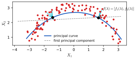
fig_14_27, principal_curve. Reproduces Hastie, Tibshirani and Friedman (2009), Figure 14.27. Download: PDF · SVGA principal surface has two parameters, \(f(\lambda_1,\lambda_2)=[f_1(\lambda_1,\lambda_2),\dots,f_p(\lambda_1,\lambda_2)]\), and step (a) uses a two-dimensional surface smoother. With a kernel smoother, step (a) has the form of the batch SOM (14.48) with the kernel weights as \(w_k\); the difference is that the principal surface gives each observation its own prototype \(f(\hat\lambda_1(x_i),\hat\lambda_2(x_i))\), while the SOM shares \(K\) prototypes, so the two agree only as \(K\) grows. The smooth parametrisation also preserves distances locally, which the SOM does not.
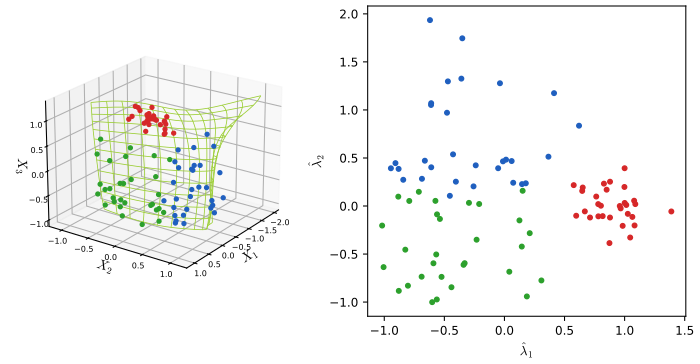
fig_14_28, principal_surface. Reproduces Hastie, Tibshirani and Friedman (2009), Figure 14.28. Download: PDF · SVG14.5.3 Spectral Clustering
pp. 544–547 K-means uses spherical (or, for mixtures, elliptical) metrics and fails for non-convex clusters such as concentric rings. Spectral clustering starts from similarities \(s_{ii'}\ge0\), for instance \(s_{ii'}=\exp(-d_{ii'}^2/c)\), and an undirected weighted graph on the \(N\) observations: in the mutual (symmetric) \(K\)-nearest-neighbour graph, \((i,i')\) is an edge with weight \(w_{ii'}=s_{ii'}\) if either point is among the other's \(K\) nearest neighbours; in the fully connected graph every pair is an edge and the scale \(c\) controls locality. The weights form the adjacency matrix \(\bW\); the degree of node \(i\) is \(g_i=\sum_{i'}w_{ii'}\), \(\bG=\diag(g_i)\), and the (unnormalised) graph Laplacian is
\[ \bL=\bG-\bW. \tag{14.63} \]Normalised versions such as \(\tilde\bL=\bI-\bG^{-1}\bW\) are also used. Spectral clustering takes the \(m\) eigenvectors of \(\bL\) with the smallest eigenvalues (ignoring the constant one), stacks them into \(\bZ\) (\(N\times m\)), and clusters the rows of \(\bZ\) with K-means.
See also (companion course): Statistical Methods for Modern Biology, Section 5.5.3 (density-based clustering), another way to find non-convex clusters.
Result 14.17 (the quadratic form of the Laplacian) p. 545, (14.64)
For every \(f\in\R^N\),
\[ f^\T\bL f=\sum_{i=1}^Ng_if_i^2-\sum_{i=1}^N\sum_{i'=1}^Nf_if_{i'}w_{ii'}=\frac12\sum_{i=1}^N\sum_{i'=1}^Nw_{ii'}(f_i-f_{i'})^2. \tag{14.64} \]So \(\bL\) is symmetric positive semidefinite, \(\bL\bone=0\), and a vector has a small quadratic form when it is nearly constant across heavy edges.
Proof
The first equality is \(f^\T\bG f-f^\T\bW f\). For the second, expand \(\frac12\sum_{i,i'}w_{ii'}(f_i^2-2f_if_{i'}+f_{i'}^2)\): by symmetry of \(\bW\) the first and third terms each give \(\frac12\sum_ig_if_i^2\), and the middle term is \(-\sum_{i,i'}w_{ii'}f_if_{i'}\). A sum of nonnegative terms is nonnegative, so \(\bL\succeq0\); and \((\bL\bone)_i=g_i-\sum_{i'}w_{ii'}=0\). ∎
Result 14.18 (the zero eigenspace is spanned by the indicators of the connected components; Exercise 14.21) pp. 545–547
If the graph has connected components \(A_1,\dots,A_m\) (with positive weights on the edges), then the eigenvalue 0 of \(\bL\) has multiplicity exactly \(m\), and its eigenspace is spanned by the indicator vectors \(\bone_{A_1},\dots,\bone_{A_m}\). In particular a connected graph has only the constant vector in its null space.
Proof
Since \(\bL\succeq0\), \(\bL f=0\) if and only if \(f^\T\bL f=0\) (if \(f^\T\bL f=0\), then \(\|\bL^{1/2}f\|^2=0\), so \(\bL f=\bL^{1/2}\bL^{1/2}f=0\)). By (14.64), \(f^\T\bL f=0\) if and only if \(f_i=f_{i'}\) for every edge \((i,i')\) with \(w_{ii'}>0\). Along any path of edges the value of \(f\) is then constant, so \(f\) is constant on each connected component: \(f=\sum_kc_k\bone_{A_k}\). Conversely each such \(f\) satisfies the condition. The \(\bone_{A_k}\) have disjoint supports, so they are linearly independent and the null space has dimension exactly \(m\). Numbering the nodes component by component makes \(\bL\) block diagonal with one connected-graph Laplacian per block, each contributing one zero eigenvalue. ∎
In practice there are strong and weak connections rather than separate components; the weak edges perturb \(\bL\) slightly, and (by continuity of eigenvalues and of the eigenspace of a group of eigenvalues well separated from the rest) the \(m\) smallest eigenvalues are small and their eigenvectors are close to the span of the indicators: nearly constant on each cluster. K-means on the rows of \(\bZ\) then sees \(m\) tight groups.
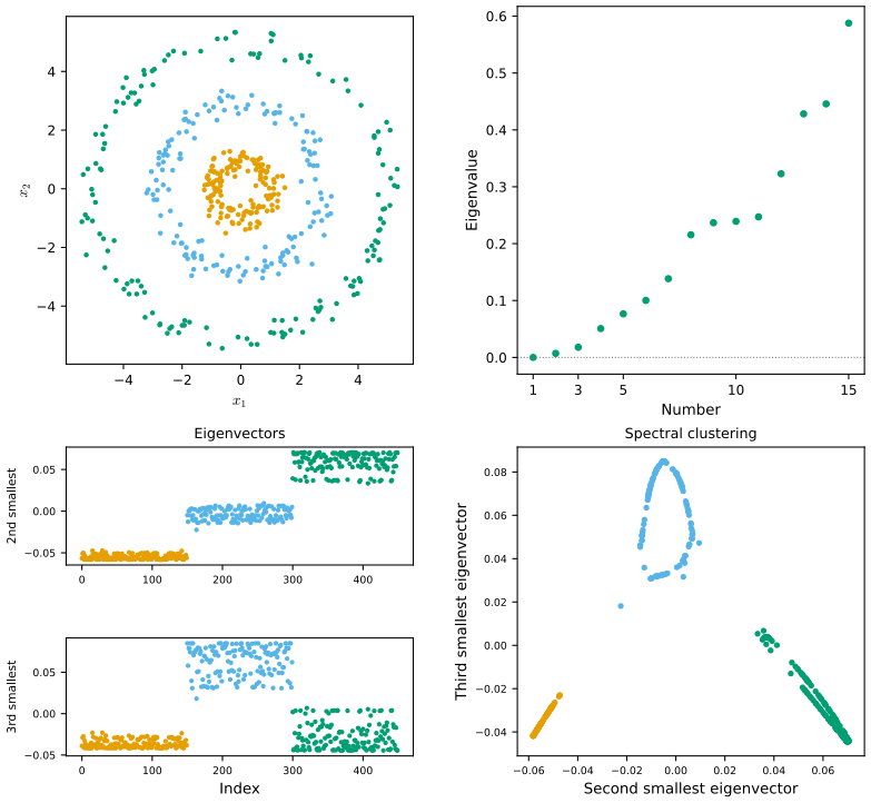
fig_14_29, spectral_embedding. Reproduces Hastie, Tibshirani and Friedman (2009), Figure 14.29. Download: PDF · SVGFilling the gap 14.11: the random-walk view, and what the normalised Laplacian optimises p. 547
Derivation
\(\bP=\bG^{-1}\bW\) has nonnegative rows summing to 1: the transition matrix of a random walk that leaves node \(i\) along edge \((i,i')\) with probability \(w_{ii'}/g_i\). The normalised Laplacian \(\tilde\bL=\bI-\bP\) has eigenpairs \(\tilde\bL v=\lambda v\iff\bL v=\lambda\bG v\), a symmetric-definite generalised problem, so the eigenvalues are real and nonnegative, with \(v^\T\bL v=\lambda\,v^\T\bG v\). For a set of nodes \(A\) with complement \(\bar A\), the stationary distribution of the walk is \(\pi_i=g_i/\sum g\), and
\[ \Pr(\text{walk moves from }A\text{ to }\bar A\given\text{it is in }A)=\frac{\sum_{i\in A,i'\in\bar A}w_{ii'}}{\sum_{i\in A}g_i}. \]Minimising the sum of this quantity over \(A\) and \(\bar A\) is the normalised cut problem, which is NP-hard. Coding the partition by \(f_i=\sqrt{\mathrm{vol}\bar A/\mathrm{vol}A}\) on \(A\) and \(-\sqrt{\mathrm{vol}A/\mathrm{vol}\bar A}\) on \(\bar A\) (\(\mathrm{vol}A=\sum_{i\in A}g_i\)) gives \(f^\T\bG\bone=0\) and \(f^\T\bL f/f^\T\bG f=\) the normalised cut. Dropping the constraint that \(f\) take two values, the minimiser of \(f^\T\bL f/f^\T\bG f\) over \(f\perp_{\bG}\bone\) is the second generalised eigenvector. So spectral clustering finds groups the walk rarely leaves, as the book says, through a continuous relaxation (von Luxburg, 2007). ∎
In practice one must choose the graph (fully connected or nearest-neighbour), \(K\) or \(c\), the number of eigenvectors and the number of clusters. The book reports good results for \(K\in[5,200]\) on its rings. On our draw, \(K=5\) already splits the graph into two components: \(\bL\) has two zero eigenvalues, the second and third eigenvectors describe that split, and the adjusted Rand index falls to 0.44; with \(K=3\) the graph falls apart into many pieces. When several eigenvalues are exactly zero, all of their eigenvectors (one per component) must be kept.
14.5.4 Kernel Principal Components
pp. 547–550 Linear principal components can be computed from the inner-product (Gram) matrix \(\bK=\bX\bX^\T\) (Section 18.5.2): with \(\bM=\bone\bone^\T/N\), compute
\[ \tilde\bK=(\bI-\bM)\bK(\bI-\bM)=\bU\bD^2\bU^\T, \tag{14.65} \]and \(\bZ=\bU\bD\). Kernel PCA (Schölkopf et al., 1999) uses the same recipe with \(\bK=\{K(x_i,x_{i'})\}\) for a kernel \(K\), i.e. linear PCA of the implicit features \(\varphi(x_i)\) with \(\langle\varphi(x_i),\varphi(x_{i'})\rangle=K(x_i,x_{i'})\). The elements of the \(m\)-th component are (up to centring) \(z_{im}=\sum_j\alpha_{jm}K(x_i,x_j)\) with \(\alpha_{jm}=u_{jm}/d_m\).
See also (companion course): Bayesian and Probabilistic Machine Learning, Result 12.14 (kernel PCA through the Gram matrix) and Result 12.15 (centring in feature space), and the kernel PCA demo.
Result 14.19 (principal components from the Gram matrix; Exercise 14.16) p. 547, (14.65)
(a) If \(\tilde\bX=(\bI-\bM)\bX=\bU\bD\bV^\T\), then \(\tilde\bK=\tilde\bX\tilde\bX^\T=\bU\bD^2\bU^\T\) and the principal components \(\tilde\bX\bV=\bU\bD\) are obtained without \(\bV\). (b) For a kernel, the number of components with \(d_m>0\) is the rank of \(\tilde\bK\) (at most \(N-1\), since \(\tilde\bK\bone=0\)). (c) \(\bZ=\tilde\bK\,\bA\) with \(\bA=\bU\bD^{-1}\), i.e. \(z_{im}=\sum_j\alpha_{jm}\tilde K(x_i,x_j)\); and a new point \(x_0\) has component \(z_{0m}=\sum_j\alpha_{jm}\tilde K(x_0,x_j)\), where \(\tilde K(x_0,\cdot)\) is the kernel row of \(x_0\) centred with the training means.
Proof
(a) \(\tilde\bX\tilde\bX^\T=\bU\bD\bV^\T\bV\bD\bU^\T=\bU\bD^2\bU^\T\), and \(\tilde\bX\bV=\bU\bD\). (b) The nonzero eigenvalues of \(\tilde\bK\) are the \(d_m^2>0\), one per column of \(\bU\) kept, so their number is \(\rank\tilde\bK\); centring kills the constant vector. (c) \(\tilde\bK\bU\bD^{-1}=\bU\bD^2\bU^\T\bU\bD^{-1}=\bU\bD\). In feature space the \(m\)-th direction is \(\nu_m=\sum_j\alpha_{jm}\tilde\varphi(x_j)\) (a unit vector, since \(\|\nu_m\|^2=\alpha_m^\T\tilde\bK\alpha_m=u_m^\T\bU\bD^2\bU^\T u_m/d_m^2=1\)), and the component of a new point is \(\langle\tilde\varphi(x_0),\nu_m\rangle=\sum_j\alpha_{jm}\tilde K(x_0,x_j)\), with \(\tilde\varphi\) the features centred by the training mean; expanding the inner products of centred features gives
\[ \tilde K(x_0,x_j)=K(x_0,x_j)-\frac1N\sum_kK(x_0,x_k)-\frac1N\sum_kK(x_k,x_j)+\frac1{N^2}\sum_{k,l}K(x_k,x_l). \]Our implementation agrees with scikit-learn's KernelPCA to \(10^{-15}\). ∎
Strictly, (b) concerns the centred matrix: the book's "the rank of \(\bK\)" can exceed the number of components by one. For the radial kernel on 150 ring points, \(\bK\) has full rank while \(\tilde\bK\) has rank 148 numerically.
The components can also be seen as functions \(g_m\) in the reproducing kernel Hilbert space \(\Hc_K\) of \(K\) (Section 5.8). The first solves
\[ \max_{g_1\in\Hc_K}\Var_\mathcal{T}\,g_1(X)\quad\text{subject to}\quad\|g_1\|_{\Hc_K}=1, \tag{14.66} \]where \(\Var_\mathcal{T}\) is the sample variance over the training data.
Result 14.20 (kernel principal component functions; Exercise 14.17) p. 548, (14.66)
With the kernel centred as in (14.65), the solution of (14.66) is \(g_1(x)=\sum_j\hat c_jK(x,x_j)\) with \(\hat c=u_1/d_1\), and its maximal variance is \(d_1^2/N\). The \(m\)-th function maximises the same criterion subject also to \(\langle g_m,g_l\rangle_{\Hc_K}=0\), \(l\lt m\), and is \(\hat c=u_m/d_m\).
Proof
Finite representation. Write \(g=\sum_jc_jK(\cdot,x_j)+g_\perp\) with \(g_\perp\) orthogonal in \(\Hc_K\) to every \(K(\cdot,x_j)\). By the reproducing property \(g_\perp(x_i)=\langle g_\perp,K(\cdot,x_i)\rangle=0\), so the values \(g(x_i)\), and hence the variance, do not depend on \(g_\perp\), while \(\|g\|^2=c^\T\bK c+\|g_\perp\|^2\). Any \(g_\perp\ne0\) uses up norm without increasing the variance (at a maximiser the norm constraint is active, since the variance scales with \(\|g\|^2\)), so \(g_\perp=0\), as in the representer theorem (Result 5.13).
The finite problem. With the centred kernel, the vector of values is \(\tilde\bK c\) (mean 0), so \(N\Var_\mathcal{T}g=c^\T\tilde\bK^2c\), and \(\|g\|^2=c^\T\tilde\bK c\). Put \(a=\bD\bU^\T c\) (only the component of \(c\) in the column space of \(\tilde\bK\) matters). Then \(c^\T\tilde\bK c=\|a\|^2\) and \(c^\T\tilde\bK^2c=\sum_md_m^2a_m^2\). Maximising \(\sum_md_m^2a_m^2\) subject to \(\|a\|=1\) gives \(a=e_1\), i.e. \(c=u_1/d_1\), value \(d_1^2\). The inner product \(\langle g_m,g_l\rangle_{\Hc_K}=c_m^\T\tilde\bK c_l=a_m^\T a_l\), so the orthogonality constraints become \(a\perp e_1,\dots,e_{m-1}\), and the maximiser is \(a=e_m\), \(c=u_m/d_m\). The values \(g_m(x_i)=(\tilde\bK u_m/d_m)_i=d_mu_{im}\) are the kernel principal components \(z_{im}\). ∎
With the radial kernel
\[ K(x,x')=\exp(-\|x-x'\|^2/c), \tag{14.67} \]\(\bK\) is the similarity matrix of spectral clustering, and \(\bW\) is its nearest-neighbour truncation. Kernel PCA takes the eigenvectors of the largest eigenvalues of \(\tilde\bK\), which are those of the smallest eigenvalues of
\[ \bI-\tilde\bK, \tag{14.68} \]a matrix like the Laplacian (14.63), except for the centring of \(\tilde\bK\) and the degrees \(g_i\) on the diagonal of \(\bG\).
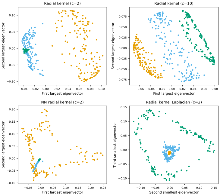
fig_14_30, kernel_pca. Reproduces Hastie, Tibshirani and Friedman (2009), Figure 14.30. Download: PDF · SVG14.5.5 Sparse Principal Components
pp. 550–552 Principal components are interpreted through their loadings \(v_j\), and sparse loadings are easier to read. With centred \(\bX\), SCoTLASS (Jolliffe et al., 2003) solves
\[ \max_v\ v^\T(\bX^\T\bX)v,\quad\text{subject to}\quad\sum_{j=1}^p|v_j|\le t,\ v^\T v=1, \tag{14.69} \]a non-convex problem. Zou et al. (2006) start instead from the reconstruction property: for one component,
\[ \min_{\theta,v}\sum_{i=1}^N\|x_i-\theta v^\T x_i\|_2^2+\lambda\|v\|_2^2+\lambda_1\|v\|_1\quad\text{subject to}\quad\|\theta\|_2=1, \tag{14.70} \]and for \(K\) components, with \(\bV\) and \(\bTh\) both \(p\times K\),
\[ \min_{\bTh,\bV}\sum_{i=1}^N\|x_i-\bTh\bV^\T x_i\|_2^2+\lambda\sum_{k=1}^K\|v_k\|_2^2+\sum_{k=1}^K\lambda_{1k}\|v_k\|_1\quad\text{subject to}\quad\bTh^\T\bTh=\bI_K. \tag{14.71} \]Result 14.21 (sparse PCA reduces to PCA without the lasso penalty) p. 550
(a) If \(\lambda=\lambda_1=0\) and \(\bS=\bX^\T\bX\) is invertible (\(N>p\), full rank), (14.70) is solved by \(v=\theta=v_1\), the first principal direction. (b) For any \(\lambda>0\) and \(\lambda_1=0\), the solution \(v\) is proportional to \(v_1\) (whatever \(N\) and \(p\); for \(p\gg N\) the ridge term makes \(v\) unique).
Proof
Since \(\|\theta\|=1\),
\[ \|x-\theta v^\T x\|^2=\|x\|^2-2(v^\T x)(\theta^\T x)+(v^\T x)^2, \]and summing over the rows, the criterion is \(\Tr\bS-2v^\T\bS\theta+v^\T(\bS+\lambda\bI)v\). For fixed \(\theta\) it is a convex quadratic in \(v\), minimised by \(v=(\bS+\lambda\bI)^{-1}\bS\theta\), with value \(\Tr\bS-\theta^\T\bS(\bS+\lambda\bI)^{-1}\bS\theta\). It remains to maximise \(\theta^\T\bS(\bS+\lambda\bI)^{-1}\bS\theta\) over unit \(\theta\). In the eigenbasis of \(\bS=\sum_jd_j^2v_jv_j^\T\) this matrix is \(\sum_j\frac{d_j^4}{d_j^2+\lambda}v_jv_j^\T\), and \(t\mapsto t^2/(t+\lambda)\) is increasing for \(t\ge0\), so the maximiser is \(\theta=v_1\) and then \(v=\frac{d_1^2}{d_1^2+\lambda}v_1\propto v_1\). With \(\lambda=0\) and \(\bS\) invertible, \(v=\theta=v_1\). When \(p>N\) and \(\lambda=0\), \(\bS\) is singular and \(v=\theta+\) anything in the null space of \(\bS\) is also optimal; \(\lambda>0\) removes this. ∎
(14.71) is not jointly convex, but it is convex in \(\bV\) for fixed \(\bTh\) and becomes a Procrustes problem in \(\bTh\) for fixed \(\bV\) (Exercise 14.12): with \(\bTh\) fixed it splits into \(K\) elastic-net regressions of the responses \(\theta_k^\T x_i\) on \(x_i\); with \(\bV\) fixed, \(\bTh=\bU\bQ^\T\) where \(\bX^\T\bX\bV=\bU\bD\bQ^\T\). The two steps are alternated. (The ordinary principal component criterion (14.50) is not jointly convex either, yet its solution is well defined.)
The book illustrates sparse PCA on shapes of the corpus callosum in 569 elderly people (Sjöstrand et al., 2007; Figures 14.31 and 14.32, the latter a photograph of a brain slice with landmarks). Those data are not available, so Figure 14.31 here applies the same method to the threes.
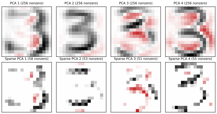
fig_14_31, sparse_pca. Reproduces the method of Hastie, Tibshirani and Friedman (2009), Figure 14.31. Download: PDF · SVG14.6 Non-negative Matrix Factorization
pp. 553–557 Non-negative matrix factorisation (Lee and Seung, 1999) approximates a non-negative \(N\times p\) data matrix by
\[ \bX\approx\bW\bH, \tag{14.72} \]with \(\bW\) (\(N\times r\)) and \(\bH\) (\(r\times p\)), \(r\le\max(N,p)\), and \(x_{ij},w_{ik},h_{kj}\ge0\). \(\bW\) and \(\bH\) maximise
\[ L(\bW,\bH)=\sum_{i=1}^N\sum_{j=1}^p\big[x_{ij}\log(\bW\bH)_{ij}-(\bW\bH)_{ij}\big], \tag{14.73} \]the log-likelihood of independent Poisson counts \(x_{ij}\) with means \((\bW\bH)_{ij}\) (the terms \(-\log x_{ij}!\) do not involve the parameters). Lee and Seung's (2001) alternating updates are
\[ w_{ik}\leftarrow w_{ik}\frac{\sum_{j=1}^ph_{kj}x_{ij}/(\bW\bH)_{ij}}{\sum_{j=1}^ph_{kj}},\qquad h_{kj}\leftarrow h_{kj}\frac{\sum_{i=1}^Nw_{ik}x_{ij}/(\bW\bH)_{ij}}{\sum_{i=1}^Nw_{ik}}. \tag{14.74} \]Result 14.22 (the multiplicative updates never decrease the likelihood; Exercise 14.23) p. 553, (14.74)
Each update in (14.74) (of \(\bW\) with \(\bH\) fixed, or of \(\bH\) with \(\bW\) fixed) is the exact maximiser of a function that minorises \(L\) at the current point. Hence \(L\) never decreases, the iterates stay non-negative, and a zero entry stays zero.
Proof
MM principle. If \(g(x,y)\le f(x)\) for all \(x,y\) and \(g(x,x)=f(x)\) (\(g\) minorises \(f\)), then \(x^{s+1}=\argmax_xg(x,x^s)\) gives
\[ f(x^{s+1})\ge g(x^{s+1},x^s)\ge g(x^s,x^s)=f(x^s). \]The minoriser. Fix the current \(\bW^s,\bH^s\) and let \(a_{ikj}=w^s_{ik}h^s_{kj}\), \(b_{ij}=\sum_ka_{ikj}=(\bW^s\bH^s)_{ij}\). Concavity of \(\log\) (Jensen's inequality with weights \(c_k=a_{ikj}/b_{ij}\), which sum to 1) gives, for any positive \(y_k\), \(\log\sum_ky_k\ge\sum_kc_k\log(y_k/c_k)\). With \(y_k=w_{ik}h_{kj}\):
\[ \log(\bW\bH)_{ij}\ \ge\ \sum_k\frac{a_{ikj}}{b_{ij}}\Big[\log w_{ik}+\log h_{kj}-\log\frac{a_{ikj}}{b_{ij}}\Big], \]with equality at \((\bW,\bH)=(\bW^s,\bH^s)\). Since \(x_{ij}\ge0\), replacing \(\log(\bW\bH)_{ij}\) in (14.73) by the right side gives, ignoring terms free of \((\bW,\bH)\),
\[ g(\bW,\bH\given\bW^s,\bH^s)=\sum_{i,j}\sum_k\Big[x_{ij}\frac{a_{ikj}}{b_{ij}}\big(\log w_{ik}+\log h_{kj}\big)-w_{ik}h_{kj}\Big]\ \le\ L(\bW,\bH), \]with equality at the current point: a minoriser.
Maximising it. For fixed \(\bH=\bH^s\), \(g\) is a sum of concave functions of the single \(w_{ik}\): \(\big(\sum_jx_{ij}a_{ikj}/b_{ij}\big)\log w_{ik}-w_{ik}\sum_jh^s_{kj}\). Setting the derivative to zero,
\[ w_{ik}=\sum_jx_{ij}a_{ikj}/b_{ij}\big/\sum_jh^s_{kj}=w^s_{ik}\sum_jh^s_{kj}x_{ij}/(\bW^s\bH^s)_{ij}\big/\sum_jh^s_{kj}, \]the first update. The same argument with \(\bW\) fixed (now at its new value) gives the second. Both factors are non-negative, so non-negativity is kept, and a zero stays zero. On the digit 2s with \(r=10\) the log-likelihood rises at every one of 100 sweeps. ∎
The algorithm can also be read as iterative proportional scaling, the classical algorithm for log-linear models: Exercise 14.24 shows that for \(r=1\) it fits the independence model of a two-way table in one sweep.
The book's Figure 14.33 compares NMF, vector quantisation (K-means) and PCA on 2429 face images (\(19\times19\) pixels) with \(r=49\); NMF learns parts of faces. That database is not available, and Figure 14.33 here does the same on the 731 training 2s with \(r=25\), which is also Exercise 14.25.
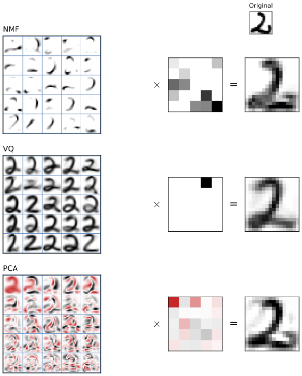
fig_14_33, vq_pca_nmf, nmf_kl. Reproduces the method of Hastie, Tibshirani and Friedman (2009), Figure 14.33. Download: PDF · SVGDonoho and Stodden (2004) point out that even an exact factorisation need not be unique, which clouds the interpretation of the parts.
Filling the gap 14.12: why NMF is not unique p. 554
Derivation
If \(\bX=\bW\bH\) with \(\bW,\bH\ge0\), then for any invertible \(r\times r\) matrix \(\bQ\) with \(\bW\bQ\ge0\) and \(\bQ^{-1}\bH\ge0\), \(\bX=(\bW\bQ)(\bQ^{-1}\bH)\) is another non-negative factorisation with the same fit. Scalings and permutations (\(\bQ\) a positive diagonal matrix times a permutation) always qualify; the question is whether other \(\bQ\) do. Geometrically, the rows of \(\bX\) must lie in the cone generated by the rows of \(\bH\) (non-negative combinations). If the data occupy a narrow cone inside the positive orthant, any pair of generators \(h_1,h_2\) in the "open space" between the data and the axes spans a cone that contains all the data, and then the coefficients \(\bW=\bX\bH^{-1}\) are non-negative: an exact factorisation for each such pair. Figure 14.34 shows two. Uniqueness needs the data to touch the boundary of the cone (Donoho and Stodden's separability conditions). ∎
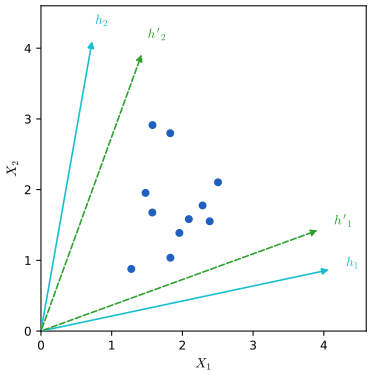
fig_14_34. Reproduces Hastie, Tibshirani and Friedman (2009), Figure 14.34. Download: PDF · SVG14.6.1 Archetypal Analysis
pp. 554–557 Archetypal analysis (Cutler and Breiman, 1994) approximates each observation by a convex combination of \(r\) prototypes that are themselves convex combinations of the observations. As in (14.72),
\[ \bX\approx\bW\bH, \tag{14.75} \]with \(w_{ik}\ge0\), \(\sum_kw_{ik}=1\), and
\[ \bH=\bB\bX, \tag{14.76} \]with \(\bB\) (\(r\times N\)) non-negative with rows summing to one. The weights minimise
\[ J(\bW,\bB)=\|\bX-\bW\bH\|^2=\|\bX-\bW\bB\bX\|^2, \tag{14.77} \]alternately in \(\bW\) and \(\bB\); each step is a convex problem (least squares over simplices), the whole is not, and the algorithm converges to a local minimum. K-means is the special case in which each row of \(\bW\) has a single one (and \(\bB\) averages the members of each cluster). Unlike NMF, archetypal analysis approximates the rows of \(\bX\) and allows \(r>p\); unlike K-means, its prototypes sit on the edge of the data.
Result 14.23 (archetypes can be taken on the boundary of the convex hull) p. 556
For \(r\ge2\), (14.77) has a minimiser whose archetypes all lie on the boundary of the convex hull of the data; moving an interior archetype outward never increases \(J\), and strictly decreases it if some observation lies outside the convex hull of the archetypes.
Proof
For fixed archetypes \(z_1,\dots,z_r\) (rows of \(\bH\)), the best \(\bW\) gives each observation its squared distance to the polytope \(P=\mathrm{conv}\{z_1,\dots,z_r\}\), so \(J=\sum_i\mathrm{dist}(x_i,P)^2\), a non-increasing function of \(P\) under inclusion. Constraint (14.76) says each \(z_k\) lies in \(\mathrm{conv}\{x_i\}\). Suppose \(z_k\) is interior. Let \(c\) be any point of \(\mathrm{conv}\{z_l:l\ne k\}\) and move \(z_k\) to \(z_k'=z_k+t(z_k-c)\), \(t>0\), until it reaches the boundary of the data hull (possible because the hull is bounded and \(z_k\) is interior). Then \(z_k=\frac1{1+t}z_k'+\frac t{1+t}c\in\mathrm{conv}\{z_k',c\}\), so the new polytope contains the old one and no distance increases. Repeat for every interior archetype. If some \(x_i\) is outside \(P\), its distance to the larger polytope is strictly smaller for suitable \(c\) (the polytope grows towards it), so at a strict minimiser no archetype is interior. ∎
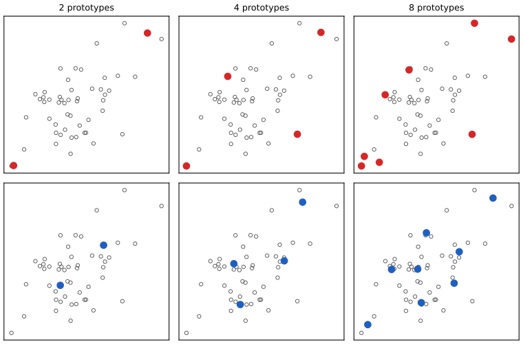
fig_14_35, archetypes. Reproduces Hastie, Tibshirani and Friedman (2009), Figure 14.35. Download: PDF · SVG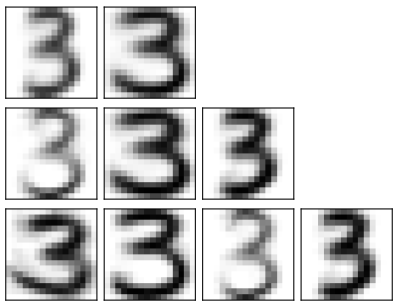
fig_14_36. Reproduces Hastie, Tibshirani and Friedman (2009), Figure 14.36. Download: PDF · SVG14.7 Independent Component Analysis and Exploratory Projection Pursuit
pp. 557–558 Multivariate data are often indirect measurements of underlying sources that cannot be observed: test scores of mental abilities, scalp electrodes of brain activity, prices of market sentiment. Factor analysis, the classical model for this, is tied to Gaussian distributions; independent component analysis relies on the sources being non-Gaussian.
14.7.1 Latent Variables and Factor Analysis
pp. 558–560 The SVD (14.54) has a latent-variable reading: with \(\bS=\sqrt N\bU\) and \(\bA^\T=\bD\bV^\T/\sqrt N\), \(\bX=\bS\bA^\T\), and for centred \(\bX\) the columns of \(\bS\) have mean 0, are uncorrelated and have unit variance. In terms of random variables,
\[ \begin{aligned}X_1&=a_{11}S_1+a_{12}S_2+\cdots+a_{1p}S_p\\ X_2&=a_{21}S_1+a_{22}S_2+\cdots+a_{2p}S_p\\ &\ \ \vdots\\ X_p&=a_{p1}S_1+a_{p2}S_2+\cdots+a_{pp}S_p,\end{aligned} \tag{14.78} \]or \(X=\bA S\) with uncorrelated unit-variance \(S_\ell\). But for any orthogonal \(\bR\),
\[ X=\bA S=\bA\bR^\T\bR S=\bA^*S^*, \tag{14.79} \]and \(\Cov(S^*)=\bR\Cov(S)\bR^\T=\bI\): the latent variables are not identified. The factor analysis model with \(q\lt p\) factors is
\[ \begin{aligned}X_1&=a_{11}S_1+\cdots+a_{1q}S_q+\varepsilon_1\\ &\ \ \vdots\\ X_p&=a_{p1}S_1+\cdots+a_{pq}S_q+\varepsilon_p,\end{aligned} \tag{14.80} \]\(X=\bA S+\varepsilon\), with \(\bA\) the \(p\times q\) loadings and uncorrelated disturbances \(\varepsilon_j\) unique to each variable. With Gaussian \(S\) and \(\varepsilon\), fitted by maximum likelihood, all parameters sit in
\[ \bSig=\bA\bA^\T+\bD_\varepsilon, \tag{14.81} \]\(\bD_\varepsilon=\diag[\Var(\varepsilon_1),\dots,\Var(\varepsilon_p)]\). The rotation problem (14.79) remains, since \(\bA\) and \(\bA\bR^\T\) give the same \(\bSig\), which leaves room for choosing "interpretable" rotations (varimax, quartimax).
See also (companion courses): Bayesian and Probabilistic Machine Learning, Definition 12.3 (factor analysis) and Result 12.13; Foundations of Deep Learning, Section 16.2.4.
Filling the gap 14.13: factor analysis models correlations, PCA models covariances p. 560
Derivation
Scale invariance. Let \(\bD_s=\diag(\sigma_1,\dots,\sigma_p)\) be the standard deviations. Pre- and post-multiplying (14.81) by \(\bD_s^{-1}\) gives the correlation matrix
\[ \bD_s^{-1}\bSig\bD_s^{-1}=(\bD_s^{-1}\bA)(\bD_s^{-1}\bA)^\T+\bD_s^{-1}\bD_\varepsilon\bD_s^{-1}: \]the same model with the rows of \(\bA\) and the uniquenesses rescaled (Exercise 14.14). The Gaussian likelihood is equivariant under such rescaling, so the maximum likelihood fit on standardised variables is the rescaled fit on raw ones. Principal components have no such property: rescaling a variable changes the directions.
Why the disturbances matter. Each \(\varepsilon_j\) can absorb all the variance of \(X_j\) that is not shared with the other variables. A variable with large variance but no correlation with the others is explained entirely by its own \(\varepsilon_j\) and does not move the factors, while it dominates the leading principal component (Exercise 14.15). ∎
When the \(\Var(\varepsilon_j)\) are all equal to \(\sigma^2\), the model is probabilistic PCA, and the maximum likelihood \(\bA\) spans the leading \(q\) principal components (Result 12.8 of the companion course).
14.7.2 Independent Component Analysis
pp. 560–565 The ICA model has the form (14.78), but with the \(S_\ell\) statistically independent, not just uncorrelated. Uncorrelatedness fixes second moments only; independence fixes all cross-moments, and those extra conditions identify \(\bA\) (up to sign and order) as long as at most one source is Gaussian. A Gaussian vector is determined by its covariance, so Gaussian sources can be recovered only up to a rotation. Without loss of generality \(X\) is whitened, \(\Cov(X)=\bI\) (via the SVD); since \(\Cov(S)=\bI\) too, \(\bA\) is then orthogonal, and ICA looks for an orthogonal \(\bA\) such that the components of \(S=\bA^\T X\) are independent (and non-Gaussian).
See also (companion courses): Bayesian and Probabilistic Machine Learning, Result 12.16 (Gaussian sources cannot be unmixed); Foundations of Deep Learning, Result 16.10 (the ICA likelihood) and the ICA unmixing demo.
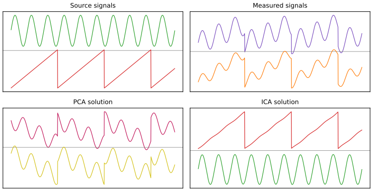
fig_14_37, fastica. Reproduces Hastie, Tibshirani and Friedman (2009), Figure 14.37. Download: PDF · SVGMany ICA methods use entropy. The differential entropy of \(Y\) with density \(g\) is
\[ H(Y)=-\int g(y)\log g(y)\,dy. \tag{14.82} \]The mutual information between the components of \(Y\),
\[ I(Y)=\sum_{j=1}^pH(Y_j)-H(Y), \tag{14.83} \]is the Kullback–Leibler divergence between the density \(g\) of \(Y\) and the product \(\prod_jg_j(y_j)\) of its marginals: zero exactly under independence. If \(\Cov(X)=\bI\) and \(Y=\bA^\T X\), then
\[ I(Y)=\sum_{j=1}^pH(Y_j)-H(X)-\log|\det\bA| \tag{14.84} \] \[ \phantom{I(Y)}=\sum_{j=1}^pH(Y_j)-H(X)\quad\text{for orthogonal }\bA. \tag{14.85} \]Result 14.24 (entropy under linear maps, and the Gaussian maximises entropy) p. 561, (14.83)–(14.85)
(a) \(I(Y)=\int g\log\big(g/\prod_jg_j\big)\ge0\), with equality if and only if the components are independent. (b) For \(Y=\bA^\T X\) with \(\bA\) invertible, \(H(Y)=H(X)+\log|\det\bA|\); this gives (14.84) and (14.85). (c) Among densities with variance \(\sigma^2\), the Gaussian has the largest entropy, \(\frac12\log(2\pi e\sigma^2)\). So, for orthogonal \(\bA\), minimising \(I(\bA^\T X)\) is minimising \(\sum_jH(Y_j)\), that is, making the unit-variance components as far from Gaussian as possible.
Proof
(a) \(-\int g\log g+\sum_j\int g_j\log g_j=\int g\log g-\int g\log\prod_jg_j\) (the marginal of \(g\) in coordinate \(j\) is \(g_j\)), which is \(\mathrm{KL}(g\,\|\prod g_j)\ge0\) by Jensen's inequality, with equality iff \(g=\prod g_j\).
(b) The density of \(Y=\bA^\T X\) is \(g_Y(y)=g_X(\bA^{-\T}y)/|\det\bA|\). Substituting \(y=\bA^\T x\) (\(dy=|\det\bA|dx\)):
\[ H(Y)=-\int g_X(x)\big[\log g_X(x)-\log|\det\bA|\big]dx=H(X)+\log|\det\bA|. \]Insert in (14.83). For orthogonal \(\bA\), \(|\det\bA|=1\), and \(\Cov(Y)=\bA^\T\bA=\bI\) as well: every \(Y_j\) has unit variance.
(c) Let \(\phi\) be the \(\N(\mu,\sigma^2)\) density with the mean and variance of \(g\). \(0\le\mathrm{KL}(g\|\phi)=-H(g)-\int g\log\phi\), and
\[ -\int g\log\phi=\frac12\log(2\pi\sigma^2)+\frac{\E(Y-\mu)^2}{2\sigma^2}=\frac12\log(2\pi e\sigma^2)=H(\phi), \]because \(\log\phi\) is a quadratic whose expectation depends only on the first two moments. So \(H(g)\le H(\phi)\), with equality iff \(g=\phi\). Since \(H(X)\) does not depend on \(\bA\), (14.85) is minimised by minimising \(\sum_jH(Y_j)\). ∎
Hyvärinen and Oja (2000) use the negentropy
\[ J(Y_j)=H(Z_j)-H(Y_j), \tag{14.86} \]with \(Z_j\) Gaussian of the same variance as \(Y_j\); by Result 14.24(c), \(J\ge0\), with equality only for Gaussian \(Y_j\). They approximate it by
\[ J(Y_j)\approx\big[\E G(Y_j)-\E G(Z_j)\big]^2, \tag{14.87} \]with \(G(u)=\frac1a\log\cosh(au)\), \(1\le a\le2\), expectations replaced by sample averages. More classical measures use the fourth moment (kurtosis), but they are less robust to outliers.
Filling the gap 14.14: where the approximation (14.87) comes from p. 562
Derivation
Standardise \(Y\) (mean 0, variance 1). Among all densities with the given values of \(\E Y\), \(\E Y^2\) and \(c=\E G(Y)\), the one with the largest entropy is \(f(y)\propto\exp(\theta_0+\theta_1y+\theta_2y^2+\theta_3G(y))\) (the same Lagrange argument as for the Gaussian). If \(Y\) is close to Gaussian, \(\theta_3\) is small; expanding the entropy of this exponential family to second order around \(\theta_3=0\), where it is the Gaussian, gives \(H(f)\approx H(\phi)-\kappa\,[c-\E G(Z)]^2\) for a constant \(\kappa>0\) (the first-order term vanishes because the Gaussian is the maximum; the coefficient of the square is half the inverse of the variance of \(G(Z)\) after removing its regression on \(Z\) and \(Z^2\)). Using this maximum-entropy density as a stand-in for the density of \(Y\), \(J(Y)\approx\kappa[\E G(Y)-\E G(Z)]^2\), which is (14.87) up to the constant. \(G\) should grow more slowly than a quadratic so that the estimate is robust; \(\log\cosh\) grows linearly. For \(Z\sim\N(0,1)\) and \(a=1\), \(\E\log\cosh Z=0.37457\). On Gaussian data the approximation is about \(10^{-6}\); on the uniform sources of Figure 14.38 it is two orders of magnitude larger. ∎
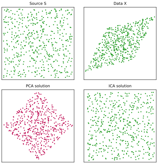
fig_14_38. Reproduces Hastie, Tibshirani and Friedman (2009), Figure 14.38. Download: PDF · SVGSo ICA looks for a sequence of orthogonal projections of the whitened data that are as non-Gaussian, and therefore as independent, as possible. It starts from a factor-analysis-like solution and rotates it, like varimax or quartimax, but with independence as the criterion.
Example: handwritten digits. Figure 14.39 compares the first five principal components of the threes with five ICA components.
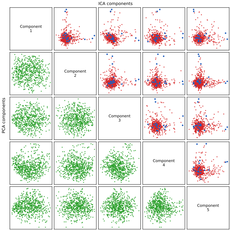
fig_14_39, digits_ica. Reproduces Hastie, Tibshirani and Friedman (2009), Figure 14.39. Download: PDF · SVG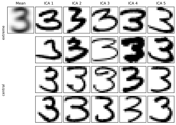
fig_14_40. Reproduces Hastie, Tibshirani and Friedman (2009), Figure 14.40. Download: PDF · SVGExample: EEG time courses. The book's Figure 14.41 (Onton and Makeig, 2006) shows nine of 100 scalp channels of an EEG recording and nine ICA components, which separate eye blinks, the cardiac pulse and frontal theta activity. The recordings are not available and the figure is not reproduced; the point is that nearby electrodes record almost the same mixture, while the independent components are temporally distinct.
14.7.3 Exploratory Projection Pursuit
p. 565 Friedman and Tukey (1974) looked for "interesting" one- or two-dimensional projections of high-dimensional data, arguing that most projections look Gaussian, and that clusters or long tails show up as non-Gaussian projections. Their projection indices measure departure from Gaussianity, and some (entropy among them) are of the form \(J(Y_j)\) with \(Y_j=a_j^\T X\). Projection pursuit usually does not force the directions to be orthogonal; Friedman (1987) transforms the data to look Gaussian in a found direction before searching for the next. With the representation used here, ICA and exploratory projection pursuit are very close. (The projection pursuit regression of Section 11.2 uses projections for prediction.)
14.7.4 A Direct Approach to ICA
pp. 565–570 Independent components have a product density
\[ f_S(s)=\prod_{j=1}^pf_j(s_j), \tag{14.88} \]and Hastie and Tibshirani (2003) estimate it directly, with each factor a tilted Gaussian
\[ f_j(s_j)=\phi(s_j)e^{g_j(s_j)}, \tag{14.89} \]\(\phi\) the standard normal density and \(g_j\) a function normalising \(f_j\) to a density. For pre-whitened \(X=\bA S\) with \(\bA\) orthogonal, the log-likelihood is
\[ \ell(\bA,\{g_j\}_1^p;\bX)=\sum_{i=1}^N\sum_{j=1}^p\big[\log\phi(a_j^\T x_i)+g_j(a_j^\T x_i)\big], \tag{14.90} \]and they maximise the penalised version
\[ \sum_{j=1}^p\Big[\frac1N\sum_{i=1}^N\big[\log\phi(a_j^\T x_i)+g_j(a_j^\T x_i)\big]-\int\phi(t)e^{g_j(t)}dt-\lambda_j\int\{g_j'''(t)\}^2dt\Big]. \tag{14.91} \]The first penalty makes the solution integrate to 1 (Silverman's device, Result 14.25); the second makes \(\hat g_j\) a quartic smoothing spline with knots at the \(s_{ij}=a_j^\T x_i\). As \(\lambda_j\to\infty\), \(\hat g_j\) tends to a quadratic and \(\hat f_j\) to \(\phi\).
Algorithm 14.3 Product density ICA (ProDenICA) p. 567
- Initialise \(\bA\) (a random Gaussian matrix, orthogonalised).
- Alternate until \(\bA\) converges:
- given \(\bA\), maximise (14.91) over each \(g_j\) separately;
- given the \(g_j\), take one step of a fixed-point algorithm towards the optimal \(\bA\).
Step 2(a) is one-dimensional semi-parametric density estimation:
\[ \frac1N\sum_{i=1}^N\big[\log\phi(s_i)+g(s_i)\big]-\int\phi(t)e^{g(t)}dt-\lambda\int\{g'''(t)\}^2dt. \tag{14.92} \]On a fine grid \(s^*_\ell\) of \(L\) points with spacing \(\Delta\), let
\[ y^*_\ell=\frac{\#\,s_i\in(s^*_\ell-\Delta/2,\,s^*_\ell+\Delta/2)}{N}, \tag{14.93} \]and approximate (14.92) by
\[ \sum_{\ell=1}^L\Big\{y^*_\ell\big[\log\phi(s^*_\ell)+g(s^*_\ell)\big]-\Delta\,\phi(s^*_\ell)e^{g(s^*_\ell)}\Big\}-\lambda\int\{g'''(s)\}^2ds, \tag{14.94} \]proportional to a penalised Poisson log-likelihood with responses \(y^*_\ell/\Delta\), mean \(\mu(s)=\phi(s)e^{g(s)}\), offset \(\log\phi(s)\) and penalty \(\lambda/\Delta\): a generalised additive spline model, fitted by Newton's method in \(O(L)\) operations. (Our implementation uses a cubic B-spline basis with a third-difference penalty set to 5 effective degrees of freedom, the default of the book's software.) Step 2(b) only involves the first terms of (14.91), and since \(\bA\) is orthogonal the \(\log\phi\) terms do not depend on \(\bA\) (Exercise 14.19), so it maximises
\[ C(\bA)=\frac1N\sum_{j=1}^p\sum_{i=1}^N\hat g_j(a_j^\T x_i), \tag{14.95} \]a log-likelihood ratio between the fitted density and the Gaussian, hence an estimate of negentropy in which each \(\hat g_j\) plays the role of the contrast \(G\) in (14.87). The fixed-point step is a modified Newton step (Exercise 14.20):
\[ a_j\leftarrow\E\big\{X\hat g_j'(a_j^\T X)-\E[\hat g_j''(a_j^\T X)]\,a_j\big\}, \tag{14.96} \]with expectations over the sample, followed by the symmetric orthogonalisation \(\bA\leftarrow(\bA\bA^\T)^{-1/2}\bA\), which for \(\bA=\bU\bD\bV^\T\) is \(\bA\leftarrow\bU\bV^\T\). FastICA uses the same update with the fixed contrast \(G\) in place of \(\hat g_j\).
Result 14.25 (the fitted tilted Gaussian is a density with mean 0 and variance 1; Exercise 14.18) p. 567
Let \(\hat g\) maximise (14.92), where the penalty \(\int(g''')^2\) does not penalise quadratics \(q(s)=\theta_0+\theta_1s+\theta_2s^2\). Then \(\hat f=\phi e^{\hat g}\) satisfies \(\int\hat f=1\), \(\int s\hat f=\frac1N\sum_is_i\) and \(\int s^2\hat f=\frac1N\sum_is_i^2\); for whitened data (mean 0, variance 1 for every \(s_i=a_j^\T x_i\)), \(\hat f\) has mean 0 and variance 1. With a second-derivative penalty only linear functions are free, and the variance condition is lost unless a free quadratic term is added back (for instance by leaving \(\theta_2s^2\) unpenalised).
Proof
Perturb \(\hat g\) to \(\hat g+\epsilon s^k\), \(k=0,1,2\). The penalty is unchanged (the third derivative of \(s^k\) is 0), and the derivative of (14.92) at \(\epsilon=0\) must vanish: \(\frac1N\sum_is_i^k-\int s^k\phi(s)e^{\hat g(s)}ds=0\). For \(k=0\) this is \(\int\hat f=1\) (this is why \(-\int\phi e^g\) appears in (14.91): the unconstrained maximiser normalises itself); for \(k=1,2\) it matches the first two sample moments. For whitened data, \(\frac1N\sum s_i=0\) and \(\frac1N\sum s_i^2=1\). Under a \((g'')^2\) penalty only \(k=0,1\) are free directions, so only the mass and the mean are matched. With the binned version (14.94), the same argument matches the binned moments, which our fit reproduces to \(10^{-12}\). ∎
The book compares ProDenICA with FastICA and KernelICA (Bach and Jordan, 2002) on 18 source distributions, measuring the error by the Amari metric between the true and estimated orthogonal mixing matrices,
\[ d(\bA_0,\bA)=\frac1{2p}\sum_{i=1}^p\Big(\frac{\sum_{j=1}^p|r_{ij}|}{\max_j|r_{ij}|}-1\Big)+\frac1{2p}\sum_{j=1}^p\Big(\frac{\sum_{i=1}^p|r_{ij}|}{\max_i|r_{ij}|}-1\Big), \tag{14.97} \]\(r_{ij}=(\bA_0\bA^{-1})_{ij}\), which is 0 exactly when \(\bA\) equals \(\bA_0\) up to permutation and scaling of its columns.
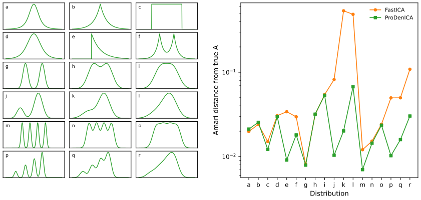
fig_14_42, prodenica, ica_simulation. Reproduces Hastie, Tibshirani and Friedman (2009), Figure 14.42. Download: PDF · SVG14.8 Multidimensional Scaling
pp. 570–572 Multidimensional scaling (MDS) places \(N\) points \(z_1,\dots,z_N\in\R^k\) so that their distances match given dissimilarities \(d_{ii'}\) (Euclidean distances between data points, or judged dissimilarities as in Section 14.3.10): only the \(d_{ii'}\) are needed. Least squares (Kruskal–Shephard) scaling minimises the stress
\[ S_M(z_1,\dots,z_N)=\sum_{i\ne i'}\big(d_{ii'}-\|z_i-z_{i'}\|\big)^2 \tag{14.98} \]by gradient descent. The Sammon mapping gives small distances more weight:
\[ S_{Sm}(z_1,\dots,z_N)=\sum_{i\ne i'}\frac{(d_{ii'}-\|z_i-z_{i'}\|)^2}{d_{ii'}}. \tag{14.99} \]Classical scaling starts from similarities, typically centred inner products \(s_{ii'}=\langle x_i-\bar x,x_{i'}-\bar x\rangle\), and minimises
\[ S_C(z_1,\dots,z_N)=\sum_{i,i'}\big(s_{ii'}-\langle z_i-\bar z,z_{i'}-\bar z\rangle\big)^2, \tag{14.100} \]which has an explicit solution in eigenvectors (Exercise 14.11). Distances can be converted to centred inner products when they are Euclidean (realisable as distances between points in some space).
See also (companion courses): Statistical Methods for Modern Biology, Result 9.1 (from squared distances to inner products), Theorem 9.2, Result 9.3 and the MDS demo; Bayesian and Probabilistic Machine Learning, Result 12.18 (classical MDS is PCA).
Result 14.26 (classical scaling; Exercise 14.11) p. 571, (14.100)
(a) If \(d_{ii'}=\|x_i-x_{i'}\|\), the matrix of centred inner products is \(\bS=-\frac12\bJ\bD^{(2)}\bJ\), with \(\bD^{(2)}=\{d_{ii'}^2\}\) and \(\bJ=\bI-\bone\bone^\T/N\). (b) Let \(\bS\) be positive semidefinite with eigenvalues \(\lambda_1\ge\lambda_2\ge\cdots\) and eigenvectors \(e_1,e_2,\dots\). The rows of \(\bE_k\bD_k\), \(\bE_k=(e_1,\dots,e_k)\), \(\bD_k=\diag(\sqrt{\lambda_1},\dots,\sqrt{\lambda_k})\), minimise (14.100), with minimum \(\sum_{m>k}\lambda_m^2\). (c) When \(\bS\) comes from data \(\bX\), these are the first \(k\) principal components \(\bU_k\bD_k\) of (14.54) (up to sign): classical scaling of Euclidean distances is PCA.
Proof
(a) With centred points \(\tilde x_i\),
\[ d_{ii'}^2=\|\tilde x_i\|^2+\|\tilde x_{i'}\|^2-2\langle\tilde x_i,\tilde x_{i'}\rangle, \]i.e. \(\bD^{(2)}=a\bone^\T+\bone a^\T-2\bS\) with \(a_i=\|\tilde x_i\|^2\). Since \(\bJ\bone=0\) and \(\bJ\bS\bJ=\bS\) (the rows and columns of \(\bS\) sum to 0), \(-\frac12\bJ\bD^{(2)}\bJ=\bS\).
(b) Let \(\bZ\) be the \(N\times k\) matrix with rows \(z_i-\bar z\); then (14.100) is \(\|\bS-\bZ\bZ^\T\|_F^2\), and \(\bZ\bZ^\T\) ranges over the positive semidefinite matrices of rank at most \(k\). For any matrix \(\bY\) of rank at most \(k\), the Eckart–Young theorem (Result 14.13(b), applied to the symmetric \(\bS=\sum_m\lambda_me_me_m^\T\), whose singular values are the \(\lambda_m\ge0\)) gives \(\|\bS-\bY\|_F^2\ge\sum_{m>k}\lambda_m^2\), attained by \(\bY=\sum_{m\le k}\lambda_me_me_m^\T=(\bE_k\bD_k)(\bE_k\bD_k)^\T\), which is of the required form. Its rows are centred because \(\bS\bone=0\) puts \(\bone\) orthogonal to the eigenvectors of positive eigenvalues.
(c) With \(\tilde\bX=\bU\bD\bV^\T\), \(\bS=\tilde\bX\tilde\bX^\T=\bU\bD^2\bU^\T\): \(e_m=u_m\), \(\sqrt{\lambda_m}=d_m\), and \(\bE_k\bD_k=\bU_k\bD_k\). ∎
If the \(d_{ii'}\) are not Euclidean, \(-\frac12\bJ\bD^{(2)}\bJ\) has negative eigenvalues; classical scaling then uses the positive part only, and the fit is approximate.
Least squares and classical scaling are metric methods; they are not equivalent (the losses differ, and least squares scaling can be a nonlinear map). Shephard–Kruskal nonmetric scaling uses only the ranks of the dissimilarities, minimising
\[ S_{NM}(z_1,\dots,z_N)=\frac{\sum_{i\ne i'}\big[\|z_i-z_{i'}\|-\theta(d_{ii'})\big]^2}{\sum_{i\ne i'}\|z_i-z_{i'}\|^2} \tag{14.101} \]over the \(z_i\) and an increasing function \(\theta\): gradient descent in the \(z_i\) for fixed \(\theta\), isotonic regression for \(\theta\) with the \(z_i\) fixed (Filling the gap 9.5 of the companion course). Like the SOM and principal surfaces, MDS gives low-dimensional coordinates; unlike them it does not fit a manifold, but because it tries to preserve all distances, points far apart are unlikely to be mapped close together.
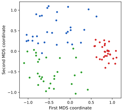
fig_14_43, classical_mds. Reproduces Hastie, Tibshirani and Friedman (2009), Figure 14.43. Download: PDF · SVG14.9 Nonlinear Dimension Reduction and Local Multidimensional Scaling
pp. 572–576 Several methods "unfold" data that lie near a low-dimensional nonlinear manifold, using only the coordinates of the points. They work best when the signal-to-noise ratio is high. Classical MDS fails on a strongly curved manifold because it judges points on opposite ends of the curve to be close (Figure 14.44).
Isomap (Tenenbaum et al., 2000) joins each point to its neighbours, approximates the geodesic distance along the manifold by the shortest path in that graph, and applies classical scaling to the graph distances. Local linear embedding (Roweis and Saul, 2000) preserves the local affine structure:
- for each \(x_i\), find its \(K\) nearest neighbours \(\Nc(i)\);
- approximate \(x_i\) by an affine combination of its neighbours, \[ \min_{w_{ik}}\Big\|x_i-\sum_{k\in\Nc(i)}w_{ik}x_k\Big\|^2, \tag{14.102} \] with \(w_{ik}=0\) for \(k\notin\Nc(i)\) and \(\sum_kw_{ik}=1\);
- find \(y_i\in\R^d\), \(d\lt p\), minimising, with the \(w_{ik}\) fixed, \[ \sum_{i=1}^N\Big\|y_i-\sum_{k=1}^Nw_{ik}y_k\Big\|^2. \tag{14.103} \]
In matrix form step 3 minimises
\[ \Tr\big[(\bY-\bW\bY)^\T(\bY-\bW\bY)\big]=\Tr\big[\bY^\T(\bI-\bW)^\T(\bI-\bW)\bY\big], \tag{14.104} \]with \(\bW\) \(N\times N\) and \(\bY\) \(N\times d\).
Result 14.27 (the two LLE steps in closed form) p. 574, (14.102)–(14.104)
(a) With the local Gram matrix \(\bC^{(i)}_{kl}=(x_k-x_i)^\T(x_l-x_i)\), \(k,l\in\Nc(i)\), the weights of (14.102) are \(w^{(i)}=\bC^{(i)-1}\bone/(\bone^\T\bC^{(i)-1}\bone)\) when \(\bC^{(i)}\) is invertible. \(\bC^{(i)}\) has rank at most \(\min(K,p)\): it is invertible (unique weights) only if \(K\le p\) and the neighbours are in general position; for \(K>p\) the usual fix is to add \(\delta\Tr(\bC^{(i)})\bI\). (b) Under the normalisation \(\bY^\T\bY=\bI\), (14.104) is minimised by the eigenvectors of \(\bM=(\bI-\bW)^\T(\bI-\bW)\) with the smallest eigenvalues, after discarding the constant vector, which has eigenvalue 0. The embedding is then centred, \(\bone^\T\bY=0\).
Proof
(a) Because the weights sum to one, \(x_i-\sum_kw_kx_k=\sum_kw_k(x_i-x_k)\), so (14.102) is \(w^\T\bC^{(i)}w\) subject to \(\bone^\T w=1\). The Lagrangian \(w^\T\bC w-2\mu(\bone^\T w-1)\) gives \(\bC w=\mu\bone\), \(w=\mu\bC^{-1}\bone\), and the constraint fixes \(\mu=1/\bone^\T\bC^{-1}\bone\). \(\bC^{(i)}=\bQ^\T\bQ\) with \(\bQ\) the \(p\times K\) matrix of differences, so its rank is at most \(\min(K,p)\). (The book's "we must have \(K\lt p\)" should be read as this condition.) The ridge term \(\delta\Tr(\bC)\bI\) makes \(\bC\) positive definite and picks the minimum-norm-like solution.
(b) Since each row of \(\bW\) sums to 1, \((\bI-\bW)\bone=0\) and \(\bM\bone=0\): the constant vector is an eigenvector with eigenvalue 0, the smallest possible since \(\bM\succeq0\). Minimising \(\Tr(\bY^\T\bM\bY)\) subject to \(\bY^\T\bY=\bI\) is minimising a sum of Rayleigh quotients over orthonormal frames, solved by the \(d\) eigenvectors of smallest eigenvalues (Ky Fan, as in Result 14.13). The constant vector would give a trivial coordinate, so it is excluded; the remaining eigenvectors are orthogonal to \(\bone\), i.e. centred. Our implementation agrees with scikit-learn's to \(4\times10^{-10}\). ∎
Local MDS (Chen and Buja, 2008) is the most direct. With \(\Nc\) the symmetric set of nearby pairs (\(i\) among the \(K\) nearest neighbours of \(i'\) or vice versa), it minimises
\[ S_L(z_1,\dots,z_N)=\sum_{(i,i')\in\Nc}\big(d_{ii'}-\|z_i-z_{i'}\|\big)^2+\sum_{(i,i')\notin\Nc}w\cdot\big(D-\|z_i-z_{i'}\|\big)^2, \tag{14.105} \]treating non-neighbours as far apart (a large distance \(D\)) but with a small weight \(w\). Letting \(w\sim1/D\) and \(D\to\infty\) gives
\[ S_L(z_1,\dots,z_N)=\sum_{(i,i')\in\Nc}\big(d_{ii'}-\|z_i-z_{i'}\|\big)^2-\tau\sum_{(i,i')\notin\Nc}\|z_i-z_{i'}\|, \tag{14.106} \]with \(\tau=2wD\): the first term preserves local structure, the second pushes non-neighbours apart.
Filling the gap 14.15: from (14.105) to (14.106) p. 576
Derivation
Expand one non-neighbour term:
\[ w(D-\|z_i-z_{i'}\|)^2=wD^2-2wD\|z_i-z_{i'}\|+w\|z_i-z_{i'}\|^2. \]The first piece does not depend on the \(z\)'s and drops out of the minimisation. Keep \(\tau=2wD\) fixed while \(D\to\infty\) (so \(w=\tau/2D\to0\)): the second piece is \(-\tau\|z_i-z_{i'}\|\), and the third, \(\frac{\tau}{2D}\|z_i-z_{i'}\|^2\), tends to 0 for bounded configurations. What remains is (14.106). The criterion is not convex, and without the neighbour term it would be unbounded below; the neighbour term holds the configuration together. ∎
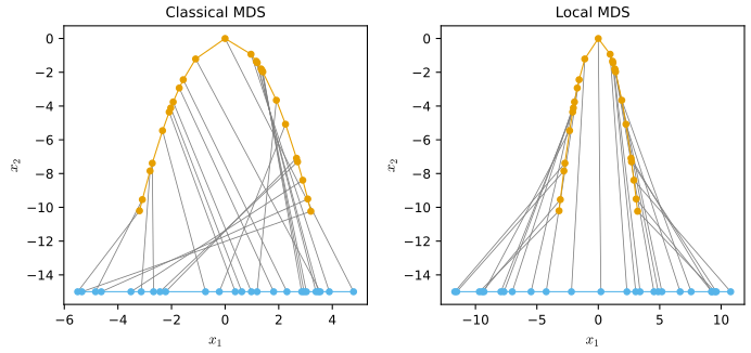
fig_14_44, local_mds. Reproduces Hastie, Tibshirani and Friedman (2009), Figure 14.44. Download: PDF · SVGThe book's Figure 14.45 shows the first two LLE coordinates of 1965 photographs of a face, which vary with pose and expression. Those images are not available; Figure 14.45 here embeds the zip-code threes instead.
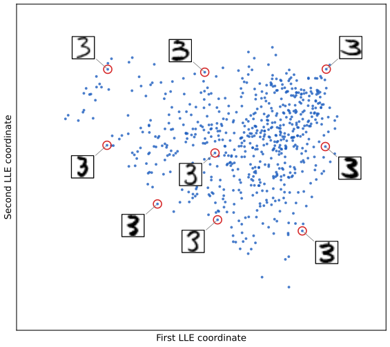
fig_14_45, lle. Reproduces the method of Hastie, Tibshirani and Friedman (2009), Figure 14.45. Download: PDF · SVGChen and Buja (2008) report that local MDS outperforms Isomap and LLE, and the methods are closely related to spectral clustering and kernel PCA: all build a local neighbourhood graph and read coordinates off eigenvectors or a stress built on it.
See also (companion course): Statistical Methods for Modern Biology, Section 9.5.2 (local, nonlinear methods) and Filling the gap 9.14 (what t-SNE optimises).
14.10 The Google PageRank Algorithm
pp. 576–578 To rank \(N\) web pages by importance, PageRank (Page et al., 1998) counts a page as important if important pages link to it, each linking page sharing one vote among its outgoing links. Let \(L_{ij}=1\) if page \(j\) links to page \(i\) and 0 otherwise, and \(c_j=\sum_iL_{ij}\) the number of pages \(j\) links to. The PageRanks are defined by
\[ p_i=(1-d)+d\sum_{j=1}^N\frac{L_{ij}}{c_j}p_j, \tag{14.107} \]with \(d=0.85\). In matrix form, with \(\be\) the vector of ones and \(\bD_c=\diag(c)\),
\[ \bp=(1-d)\be+d\,\bL\bD_c^{-1}\bp. \tag{14.108} \]With the normalisation \(\be^\T\bp=N\) (average PageRank 1) this is
\[ \bp=\big[(1-d)\be\be^\T/N+d\,\bL\bD_c^{-1}\big]\bp=\bA\bp, \tag{14.109} \]and the PageRanks are found by the power method:
\[ \bp_k\leftarrow\bA\bp_{k-1};\qquad \bp_k\leftarrow N\frac{\bp_k}{\be^\T\bp_k}. \tag{14.110} \]The random-surfer reading: the surfer follows a random outgoing link with probability \(d\) and jumps to a page chosen at random with probability \(1-d\); \(\bA\) is the transition matrix of this Markov chain (columns sum to one), and \(\bp/N\) is its stationary distribution.
Result 14.28 (existence, uniqueness and positivity of PageRank; convergence of the power method) pp. 577–578
Assume every page has at least one outgoing link (\(c_j\ge1\)) and \(0\le d\lt1\). Then:
- (14.108) has exactly one solution, \(\bp=(1-d)\sum_{k\ge0}d^k(\bL\bD_c^{-1})^k\be\); every \(p_i\ge1-d\) (with equality exactly for pages without incoming links), and \(\be^\T\bp=N\) automatically (Exercise 14.22(a)).
- \(\bp\) is, up to scale, the only eigenvector of \(\bA\) for the eigenvalue 1; every other eigenvalue \(\lambda\) of \(\bA\) has \(|\lambda|\le d\).
- From any \(\bp_0\) with \(\be^\T\bp_0=N\), the iterates (14.110) satisfy \(\|\bp_k-\bp\|_1\le d^k\|\bp_0-\bp\|_1\).
Proof
Write \(\bP=\bL\bD_c^{-1}\). Its entries are non-negative and each column sums to \(\sum_iL_{ij}/c_j=1\): \(\be^\T\bP=\be^\T\). The induced \(\ell_1\) norm of a matrix is its largest absolute column sum, so \(\|\bP v\|_1\le\|v\|_1\) for all \(v\).
(1) (14.108) is \((\bI-d\bP)\bp=(1-d)\be\). Since \(\|d\bP\|_1=d\lt1\), the Neumann series \(\sum_kd^k\bP^k\) converges and is the inverse of \(\bI-d\bP\): the solution exists, is unique and has the stated form. All terms are non-negative and the \(k=0\) term is \((1-d)\be\), so \(p_i\ge1-d\); by (14.107), \(p_i=1-d\) exactly when \(\sum_jL_{ij}p_j/c_j=0\), i.e. no page links to \(i\) (all \(p_j>0\)). Multiplying (14.108) by \(\be^\T\): \(\be^\T\bp=(1-d)N+d\,\be^\T\bp\), so \(\be^\T\bp=N\).
(2) For \(\be^\T\bp=N\), \(\bA\bp=(1-d)\be+d\bP\bp\), so \(\bA\bp=\bp\) is (14.108) and, by (1), has the single normalised solution; an eigenvector for the eigenvalue 1 with \(\be^\T v=0\) would satisfy \(d\bP v=v\), impossible for \(v\ne0\) since \(\|d\bP v\|_1\le d\|v\|_1\). Any eigenvector \(v\) of another eigenvalue \(\lambda\ne1\) has \(\be^\T v=0\), because \(\be^\T\bA=\be^\T\) gives \(\be^\T v=\be^\T\bA v=\lambda\be^\T v\). Then \(\bA v=d\bP v\) (the first term of \(\bA\) annihilates \(v\)), and \(|\lambda|\|v\|_1=\|d\bP v\|_1\le d\|v\|_1\). (Complex eigenvectors are handled the same way with the \(\ell_1\) norm on \(\mathbb{C}^N\).)
(3) \(\be^\T\bA=\be^\T\) means \(\bA\) preserves the sum, so with \(\be^\T\bp_0=N\) the normalisation in (14.110) does nothing and \(\bp_k=\bA^k\bp_0\). Then \(\bp_k-\bp=\bA(\bp_{k-1}-\bp)=d\bP(\bp_{k-1}-\bp)\), since the difference sums to zero, and \(\|\bp_k-\bp\|_1\le d\|\bp_{k-1}-\bp\|_1\). ∎
This is the Perron–Frobenius theorem for this particular positive, column-stochastic matrix: \(\bA\) has all entries at least \((1-d)/N>0\), so the chain is irreducible and aperiodic, and its stationary distribution is unique and positive (Brémaud, 1999). The argument above gives the explicit rate \(d\). With \(d=1\) the conclusions can fail: if the web splits into two parts with no links between them, every mixture of the two parts' stationary vectors is a fixed point.
Note on the book: the \((1-d)/N\) version is the same Markov chain p. 577
The book says that putting \((1-d)/N\) in place of \((1-d)\) in (14.107) fits the random-surfer interpretation better, and that (14.107) "also corresponds to an irreducible, aperiodic Markov chain, with different transition probabilities". When every \(c_j\ge1\), both versions lead to the same matrix \(\bA\) of (14.109): if \(\bp\) solves (14.108), then \(\bp/N\) solves \(\bp=(1-d)\be/N+d\bL\bD_c^{-1}\bp\), and both are the fixed point of \(\bA\) normalised to sum \(N\) or 1. The chain is the same; only the scale of the answer differs (numerically, the two solutions differ by the factor \(N\) to \(10^{-12}\) on both of the book's networks). A page with no outgoing links (\(c_j=0\)) makes \(\bD_c^{-1}\) undefined; the usual fix, used in the demo, treats it as linking to every page.
For the network of Figure 14.46 the link matrix is
\[ \bL=\begin{pmatrix}0&0&1&0\\1&0&0&0\\1&1&0&1\\0&0&0&0\end{pmatrix}, \tag{14.111} \]with \(c=(2,1,1,1)\), and the PageRanks are \(\hat\bp=(1.49,0.78,1.58,0.15)\). Page 4 has no incoming links and gets the minimum \(1-d=0.15\).
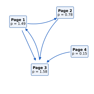
fig_14_46, pagerank. Reproduces Hastie, Tibshirani and Friedman (2009), Figure 14.46 (the web pages are drawn as boxes). Download: PDF · SVGExercises
All 25 exercises of Chapter 14 (Hastie, Tibshirani and Friedman, 2009, pp. 579–584), restated in my own words, with complete solutions (hidden). Computations use the chapter's code (exercises() and the exercise_14_* functions).
Exercise 14.1 (weights for clustering). Show that the weighted squared Euclidean distance
\[ d_e^{(w)}(x_i,x_{i'})=\sum_lw_l(x_{il}-x_{i'l})^2/\sum_lw_l \]equals the ordinary squared distance between \(z_i\) and \(z_{i'}\),
\[ d_e^{(w)}(x_i,x_{i'})=d_e(z_i,z_{i'})=\sum_{l=1}^p(z_{il}-z_{i'l})^2, \tag{14.112} \]where
\[ z_{il}=x_{il}\cdot\Big(\frac{w_l}{\sum_{l=1}^pw_l}\Big)^{1/2}. \tag{14.113} \]Solution
With \(s_l=(w_l/\sum_mw_m)^{1/2}\), \(z_{il}-z_{i'l}=s_l(x_{il}-x_{i'l})\), so
\[ \sum_l(z_{il}-z_{i'l})^2=\sum_ls_l^2(x_{il}-x_{i'l})^2=\sum_lw_l(x_{il}-x_{i'l})^2/\sum_mw_m. \]Hence any method that uses squared Euclidean distance (K-means in particular) can use weighted distance by rescaling each variable by \(\sqrt{w_l}\) first; Figure 14.5 is an example with \(w_l=1/[2\,\mathrm{var}(X_l)]\).
Exercise 14.2. Consider the mixture \(g(x)=\sum_{k=1}^K\pi_kg_k(x)\) (14.114) with \(g_k=\N(\mu_k,\bI\sigma^2)\) (the book prints \(\bL\cdot\sigma^2\), a typo for \(\bI\cdot\sigma^2\)), \(\pi_k\ge0\), \(\sum_k\pi_k=1\). (1) Write down the log-likelihood of data \(x_1,\dots,x_N\). (2) Derive an EM algorithm. (3) Show that if \(\sigma\) is known and \(\sigma\to0\), EM coincides in a sense with K-means.
\[ g(x)=\sum_{k=1}^K\pi_kg_k(x) \tag{14.114} \]Solution
(1)
\[ \ell(\theta)=\sum_{i=1}^N\log\sum_{k=1}^K\pi_k(2\pi\sigma^2)^{-p/2}\exp(-\|x_i-\mu_k\|^2/2\sigma^2). \](2) Introduce the latent labels \(\Delta_{ik}=1\) if \(x_i\) came from component \(k\). The complete-data log-likelihood is
\[ \sum_i\sum_k\Delta_{ik}[\log\pi_k-\frac p2\log(2\pi\sigma^2)-\|x_i-\mu_k\|^2/2\sigma^2]. \]E-step: replace \(\Delta_{ik}\) by its conditional expectation, the responsibility \(r_{ik}=\pi_kg_k(x_i)/\sum_l\pi_lg_l(x_i)\). M-step: maximise \(\sum_{i,k}r_{ik}[\dots]\): for the means, \(\mu_k=\sum_ir_{ik}x_i/\sum_ir_{ik}\); for the weights, with a Lagrange multiplier for \(\sum\pi_k=1\), \(\pi_k=\frac1N\sum_ir_{ik}\); for \(\sigma^2\) (if unknown), \(\sigma^2=\frac1{Np}\sum_{i,k}r_{ik}\|x_i-\mu_k\|^2\). Each iteration does not decrease \(\ell\) (Result 8.8).
(3) This is Result 14.7: as \(\sigma\to0\), \(r_{ik}\to1\) for the closest mean and 0 otherwise, so the E-step becomes the assignment step (14.34) and the M-step for the means becomes (14.32). On the data of Figure 14.4, EM with \(\sigma=0.1\) from the start of Figure 14.6 ends at the K-means centres and partition exactly, and with \(\sigma=0.3\) the centres differ by at most \(10^{-3}\). (The weights \(\pi_k\) enter the limit only through ties.)
Exercise 14.3. In Section 14.2.6, CART or PRIM are used to find generalised association rules. Show that a problem arises with either method when the reference data are generated from the product of the marginals, i.e. by randomly permuting each variable, and propose remedies.
Solution
The problem is Result 14.3: every region defined by a single variable contains exactly as many reference points as data points, so every first split of CART has zero impurity decrease and every first peel of PRIM leaves the target mean at exactly \(\tfrac12\). Associations show up only in regions defined by two or more variables, which a greedy one-variable-at-a-time search cannot reach on its first step; the first split is decided by ties (on the demographics data the first CART split has Gini decrease exactly 0), and later splits inherit that arbitrariness.
Remedies: (i) search over pairs of variables at the first step (two-step look-ahead in CART, or peeling two variables at a time in PRIM); (ii) use a method that models interactions without a greedy marginal start, for instance boosting with depth-2 trees or logistic regression with pairwise interaction terms, and read the high-\(\hat\mu\) regions from the fit; (iii) draw the reference sample by sampling each column with replacement, or from smoothed marginals, which breaks the exact ties but leaves the expected marginal gain at 0, so it is only a partial cure; (iv) use a different reference (the uniform), at the price of rediscovering marginally frequent values (14.17).
Exercise 14.4. Cluster the demographics data of Table 14.1 with a classification tree: make a reference sample of the same size by permuting each feature, fit a tree to data (class 1) against reference (class 0), and describe the terminal nodes with the highest class-1 probability. Compare with PRIM (Section 14.2.7) and with K-means on the same data.
Solution
Tree (depth 6, at least 100 observations per leaf) on the 14 coded inputs of the 6876 complete rows against their permuted copy (
market_tree); the first split has zero gain, as Exercise 14.3 predicts, but deeper splits find structure. The four leaves with the highest proportion of real data:- lives in a house, lives with parents or family, aged 14–24, single and not in a dual-income couple: class-1 proportion 0.93, data support 14.5%;
- not in a house, lives with family, aged 14–24, single, income below $10,000: 0.93, support 2.2%;
- lives in a house, owns it, married, aged over 24, dual income: 0.89, support 22.7%;
- lives in a condominium, owns it, household of at most two, college graduate: 0.84, support 1.5%.
These are the same kinds of item sets as the book's PRIM results (married home owners in houses; young singles living with their family). K-means with \(K=4\) on the 50 dummies gives four segments of 34%, 23%, 25% and 18%: renters in apartments in small households with lower income; young singles (students) living with their family; older home owners without children and with higher income; married couples with children. K-means partitions everybody, including people in no dense region, while the tree (or PRIM) reports only the high-density regions with their support.
Exercise 14.5. Generate three classes of 30 points in \(\R^3\) near the unit sphere: class 1 with \(\theta\sim U(-\pi/8,\pi/8)\), \(\phi\sim U(0,2\pi)\); class 2 with \(\theta\sim U(\pi/2-\pi/4,\pi/2+\pi/4)\), \(\phi\sim U(-\pi/4,\pi/4)\); class 3 with \(\theta,\phi\sim U(\pi/2-\pi/4,\pi/2+\pi/4)\); point \((\sin\theta\cos\phi,\sin\theta\sin\phi,\cos\theta)\) plus independent normal noise of standard deviation 0.6 per coordinate. Fit a SOM with the learning rates of the text, and K-means, and compare with the text.
Solution
The classes are centred near \((0,0,1)\), \((1,0,0)\) and \((0,1,0)\). The code is
half_sphereandsom_online(Section 14.4: \(5\times5\) grid on the principal component plane, \(R=2\), \(\alpha\) from 1 to 0, 40 passes). With noise sd 0.6 the SOM ends with reconstruction error 34.1 and K-means with 25 centres 15.0, out of a total sum of squares of 186: the clusters overlap heavily and the map is mostly noise. With sd 0.1 the numbers are 5.56, 2.27 and 74.1, and Figures 14.15–14.18 look like the book's; see the note on the noise level. In both cases the SOM error is within a factor of about 2.5 of K-means, so the two-dimensional constraint is reasonable, and the SOM separates the three classes on the grid while hiding that class 1 is the tightest.Exercise 14.6. Implement K-means and a SOM with prototypes on a two-dimensional grid, apply them to the columns (samples) of the microarray data with \(K=2,5,10,20\), and show that as the SOM neighbourhood shrinks the SOM solution approaches the K-means solution.
Solution
exercise_14_6: grids \(1\times2\), \(1\times5\), \(2\times5\), \(4\times5\), started on the principal component plane; batch SOM (14.48) with a Gaussian neighbourhood of width \(r=2,1,0.5,0.2,0.05\) grid units, each run to convergence from the previous one. Reconstruction errors (the K-means value is the best of 30 random starts):K r = 2 r = 1 r = 0.5 r = 0.2 r = 0.05 K-means 2 264452 255737 241185 239555 239555 236482 5 248967 226574 198066 192420 192420 194612 10 244864 213260 178014 168335 168335 158435 20 220158 182519 152234 137426 137426 114441 The error falls monotonely as the neighbourhood shrinks. Once the Gaussian weights of the neighbours are negligible (\(r\le0.2\)), the batch SOM update is exactly a Lloyd step (Result 14.11), and the final SOM partition is a fixed point of K-means: starting K-means from the SOM prototypes changes no assignment. Whether it is the best K-means solution depends on the start: for \(K=5\) the SOM path ends below the best of 30 random K-means starts, for \(K=20\) above it.
Exercise 14.7. Derive (14.51) and (14.52). Show that \(\hat\mu\) is not unique and characterise the family of equivalent solutions.
Solution
This is Result 14.12: the minimisers are \(\mu=\bar x+\bV_qc\) with \(\lambda_i=\bV_q^\T(x_i-\bar x)-c\), \(c\in\R^q\) arbitrary; all give the same fitted values \(\bar x+\bV_q\bV_q^\T(x_i-\bar x)\). Moving \(\mu\) within the fitted affine subspace and shifting every \(\lambda_i\) back describes the same subspace. The choice \(c=0\) makes the \(\hat\lambda_i\) average to 0.
Exercise 14.8. Derive the solution (14.57) of the Procrustes problem (14.56), and the solution of the problem with scaling (14.58).
Solution
This is Result 14.14: \(\hat\bR=\bU\bV^\T\) from \(\tilde\bX_1^\T\tilde\bX_2=\bU\bD\bV^\T\), \(\hat\mu=\bar x_2-\hat\bR^\T\bar x_1\) (see the note on the transpose), and with scaling the same rotation and \(\hat\beta=\Tr(\bD)/\|\tilde\bX_1\|_F^2\). The key step is \(\max_{\bR}\Tr(\bR^\T\bU\bD\bV^\T)=\max\Tr(\bQ\bD)=\Tr\bD\) over orthogonal \(\bQ=\bV^\T\bR^\T\bU\), attained at \(\bQ=\bI\).
Exercise 14.9. Write an algorithm to solve
\[ \min_{\{\beta_\ell,\bR_\ell\}_1^L,\bM}\sum_{\ell=1}^L\|\beta_\ell\bX_\ell\bR_\ell-\bM\|_F^2, \tag{14.115} \]apply it to the three S's and compare with Figure 14.26.
Solution
As stated, (14.115) is minimised by \(\beta_\ell=0\), \(\bM=0\); a normalisation is needed, for instance fixing \(\|\bM\|_F\) (we fix it at the size of the first centred shape). Algorithm (
procrustes_average(..., scaling=True)): centre each \(\bX_\ell\); start with \(\bM\) = the first shape; (1) for each \(\ell\), solve the Procrustes problem with scaling of \(\bX_\ell\) onto \(\bM\) (Result 14.14): \(\bX_\ell^\T\bM=\bU\bD\bV^\T\), \(\bR_\ell=\bU\bV^\T\), \(\beta_\ell=\Tr\bD/\|\bX_\ell\|_F^2\); (2) set \(\bM\) to the average of the \(\beta_\ell\bX_\ell\bR_\ell\), rescaled to the fixed size; repeat. For the three S's the scales are 0.964, 1.000 and 0.973: the three signatures have almost the same size, so the scaled average is almost the plain Procrustes average of Figure 14.26 (the shapes are rescaled by at most 4%).Exercise 14.10. Derive the solution of the affine-invariant average problem (14.60), apply it to the three S's and compare with Exercise 14.9.
Solution
This is Result 14.15: \(\bM\) = the two leading eigenvectors of \(\bar\bH=\frac13\sum_\ell\bH_\ell\), \(\hat\bA_\ell=(\bX_\ell^\T\bX_\ell)^{-1}\bX_\ell^\T\bM\). For the S's the leading eigenvalues of \(\bar\bH\) are 0.971 and 0.898 (the third is 0.098), and the minimum of (14.60) is 0.393 under \(\bM^\T\bM=\bI\). The affine average is an orthonormal "shape" (the scale is fixed by \(\bM^\T\bM=\bI\)); mapped back by \(\hat\bA_\ell^{-1}\), it matches each S at least as closely as the Procrustes average, because affine maps include rotations and scalings, and it differs from it mainly by allowing shear: the slant of each signature is absorbed by \(\bA_\ell\).
Exercise 14.11 (classical multidimensional scaling). Let \(\bS\) be the centred inner-product matrix with elements \(\langle x_i-\bar x,x_j-\bar x\rangle\), with largest eigenvalues \(\lambda_1>\dots>\lambda_k\) and eigenvectors \(\bE_k\), and \(\bD_k=\diag(\sqrt{\lambda_1},\dots,\sqrt{\lambda_k})\). Show that the solutions \(z_i\) of the classical scaling problem (14.100) are the rows of \(\bE_k\bD_k\).
Solution
This is Result 14.26(b): (14.100) is \(\|\bS-\bZ\bZ^\T\|_F^2\) over centred \(N\times k\) matrices \(\bZ\), and by the Eckart–Young theorem the best approximation of the positive semidefinite \(\bS\) of rank at most \(k\) is \(\sum_{m\le k}\lambda_me_me_m^\T=(\bE_k\bD_k)(\bE_k\bD_k)^\T\). The solution is unique up to an orthogonal transformation of the rows (\(\bZ\bQ\) has the same \(\bZ\bZ^\T\)), as it must be for a configuration known only through inner products.
Exercise 14.12. For the sparse PCA criterion (14.71): (1) show that with \(\bTh\) fixed, solving for \(\bV\) is \(K\) separate elastic-net regressions with responses the \(K\) elements of \(\bTh^\T x_i\); (2) show that with \(\bV\) fixed, solving for \(\bTh\) is a reduced-rank Procrustes problem,
\[ \max_{\bTh}\Tr(\bTh^\T\bM)\quad\text{subject to}\quad\bTh^\T\bTh=\bI_K, \tag{14.116} \]with \(\bM\) and \(\bTh\) both \(p\times K\), \(K\le p\); if \(\bM=\bU\bD\bQ^\T\) is the SVD of \(\bM\), the optimal \(\bTh\) is \(\bU\bQ^\T\).
Solution
(1) Using \(\bTh^\T\bTh=\bI\),
\[ \|x-\bTh\bV^\T x\|^2=\|x\|^2-2\sum_k(\theta_k^\T x)(v_k^\T x)+\sum_k(v_k^\T x)^2, \]while
\[ \sum_k(\theta_k^\T x-v_k^\T x)^2=\sum_k(\theta_k^\T x)^2-2\sum_k(\theta_k^\T x)(v_k^\T x)+\sum_k(v_k^\T x)^2. \]The two differ by \(\|x\|^2-\|\bTh^\T x\|^2\), which does not involve \(\bV\). So (14.71) equals, up to a constant,
\[ \sum_{k=1}^K\big[\sum_i(\theta_k^\T x_i-v_k^\T x_i)^2+\lambda\|v_k\|_2^2+\lambda_{1k}\|v_k\|_1\big]: \]\(K\) independent elastic-net problems, regressing the response \(\theta_k^\T x_i\) on \(x_i\).
(2) With \(\bV\) fixed, the only term of (14.71) involving \(\bTh\) is \(-2\sum_ix_i^\T\bTh\bV^\T x_i=-2\Tr(\bTh^\T\bX^\T\bX\bV)\) (the quadratic term \(\|\bTh\bV^\T x\|^2=\|\bV^\T x\|^2\) does not depend on \(\bTh\)). So we maximise \(\Tr(\bTh^\T\bM)\) with \(\bM=\bX^\T\bX\bV\). With \(\bM=\bU\bD\bQ^\T\) (\(\bU\) \(p\times K\), \(\bD\), \(\bQ\) \(K\times K\)), \(\Tr(\bTh^\T\bU\bD\bQ^\T)=\Tr(\bQ^\T\bTh^\T\bU\bD)=\sum_kG_{kk}d_k\) with \(\bG=\bQ^\T\bTh^\T\bU\). \(\bG\) is a product of matrices of operator norm at most 1, so \(|G_{kk}|\le1\) and the trace is at most \(\sum_kd_k\), attained when \(\bG=\bI\), i.e. \(\bTh=\bU\bQ^\T\) (which satisfies \(\bTh^\T\bTh=\bQ\bU^\T\bU\bQ^\T=\bI\)). Numerically, for a random \(8\times3\) \(\bM\), \(\Tr(\bTh^\T\bM)\) at \(\bU\bQ^\T\) equals the sum of the singular values (10.425), while the best of 5000 random orthonormal frames reaches 6.71. With \(\lambda_1=0\) the alternation returns the principal directions of the threes (\(|\cos|=1\) to nine digits).
Exercise 14.13. Generate 200 points near a helix: \(X_1=\cos s+0.1Z_1\), \(X_2=\sin s+0.1Z_2\), \(X_3=s+0.1Z_3\), with \(s\) 200 equally spaced values in \([0,2\pi]\) and \(Z_j\) independent standard normal. (a) Fit a principal curve and compare its coordinate functions with \(\cos s\), \(\sin s\), \(s\). (b) Fit a SOM and see whether it discovers the helix.
Solution
(a)
principal_curve(local linear smoother, span 0.08, started from the first principal component line, which is nearly the helix axis): the fitted arc-length orders the points as \(s\) does (Spearman correlation 0.9993), and after matching \(\hat\lambda\) to \(s\), the root mean squared differences of the coordinate functions from \(\cos s\), \(\sin s\) and \(s\) are 0.089, 0.092 and 0.072, about the noise level 0.1: the curve recovers the helix. (b) A one-dimensional SOM with 20 prototypes (40 passes, \(\alpha\) from 1 to 0, radius from 20/3 to 1) orders its prototypes along the helix (Spearman correlation 1.0 between prototype index and the average \(s\) of the points it wins), with residual sum of squares 9.27: the chain of prototypes traces the helix. A two-dimensional SOM grid would also follow it but fold, as in Figure 14.17, since the data are intrinsically one-dimensional.Exercise 14.14. Pre- and post-multiply (14.81) by the diagonal matrix of inverse standard deviations of the \(X_j\), and so obtain an equivalent decomposition of the correlation matrix in which \(\bA\) is simply rescaled.
Solution
Let \(\bD_s=\diag(\sigma_1,\dots,\sigma_p)\), \(\sigma_j^2=\Sigma_{jj}\). Then the correlation matrix is
\[ \bD_s^{-1}\bSig\bD_s^{-1}=(\bD_s^{-1}\bA)(\bD_s^{-1}\bA)^\T+\bD_s^{-1}\bD_\varepsilon\bD_s^{-1}: \]a factor model with loadings \(a_{jl}/\sigma_j\) (row \(j\) of \(\bA\) divided by \(\sigma_j\)) and uniquenesses \(\Var(\varepsilon_j)/\sigma_j^2\), still diagonal. Since \(\sigma_j^2=\sum_la_{jl}^2+\Var(\varepsilon_j)\), each standardised communality plus uniqueness equals 1. (The book says "inverse variances"; the matrix needed is that of inverse standard deviations.) See Filling the gap 14.13.
Exercise 14.15. Generate 200 observations of
\[ X_1\sim Z_1,\qquad X_2=X_1+0.001\cdot Z_2,\qquad X_3=10\cdot Z_3, \tag{14.117} \]with \(Z_1,Z_2,Z_3\) independent standard normal. Compute the leading principal component and factor analysis directions, and show that the principal component aligns with the high-variance \(X_3\), while the leading factor ignores the uncorrelated \(X_3\) and picks up the correlated \(X_1+X_2\).
Solution
Population covariance: \(\Var X_1=\Var X_2\approx1\), \(\Cov(X_1,X_2)\approx1\), \(\Var X_3=100\), \(X_3\) uncorrelated with the others. The leading eigenvector of the covariance is \(e_3\) (eigenvalue 100 against 2 for \((1,1,0)/\sqrt2\)): our sample gives \(v_1=(0.013,0.013,0.9998)\). The one-factor model \(\bSig=aa^\T+\bD_\varepsilon\) can reproduce \(\Cov(X_1,X_2)=1\) only through \(a_1a_2\approx1\), while \(X_3\)'s variance is free to go into \(\Var\varepsilon_3\). Maximum likelihood (our
factor_analysis, profile likelihood) gives loadings \((0.993,0.993,1.38)\) and uniquenesses \((10^{-6},\ 1.7\times10^{-8},\ 106.8)\): standardised loadings about \((1.00,1.00,0.13)\). The factor is \(X_1\approx X_2\), and \(X_3\) is almost entirely its own disturbance. The solution is a Heywood case (uniquenesses at the boundary 0), which is typical when two variables are almost identical. (scikit-learn's FactorAnalysis stops at a much worse local optimum on these data, with a large loading on \(X_3\); maximising the likelihood properly matters.)Exercise 14.16. For kernel PCA (Section 14.5.4), argue that the number \(M\) of components equals the rank of \(\bK\), the number of nonzero elements of \(\bD\); show that \(z_{im}=\sum_j\alpha_{jm}K(x_i,x_j)\) (up to centring) with \(\alpha_{jm}=u_{jm}/d_m\); and show that a new point \(x_0\) maps to \(z_{0m}=\sum_j\alpha_{jm}K(x_0,x_j)\).
Solution
This is Result 14.19. The count is the rank of the centred \(\tilde\bK\), which is at most \(N-1\) and can be one less than \(\rank\bK\); \(\bZ=\tilde\bK\bU\bD^{-1}=\bU\bD\); and a new point uses its kernel row centred with the training means. On 150 ring points with the radial kernel, \(\tilde\bK\bU\bD^{-1}\) equals \(\bU\bD\) to \(2\times10^{-15}\), the projections of 50 new points agree with scikit-learn's KernelPCA to \(10^{-15}\), and \(\rank\tilde\bK=148\).
Exercise 14.17. Show that with \(g_1(x)=\sum_jc_jK(x,x_j)\) the solution of (14.66) is \(\hat c_j=u_{j1}/d_1\), and that the later principal component functions are defined similarly.
Solution
This is Result 14.20: with \(a=\bD\bU^\T c\), the variance is \(\sum_md_m^2a_m^2/N\) and the squared norm is \(\|a\|^2\), so the maximiser is \(a=e_1\), \(c=u_1/d_1\); the orthogonality constraints \(\langle g_m,g_l\rangle_{\Hc_K}=a_m^\T a_l=0\) give \(c=u_m/d_m\) for the \(m\)-th function.
Exercise 14.18. For the regularised log-likelihood
\[ \frac1N\sum_{i=1}^N\big[\log\phi(s_i)+g(s_i)\big]-\int\phi(t)e^{g(t)}dt-\lambda\int\{g'''(t)\}^2dt, \tag{14.118} \]whose solution is a quartic smoothing spline \(\hat g=\hat q+\hat q_\perp\) with \(q(s)=\theta_0+\theta_1s+\theta_2s^2\) in the null space of the penalty, show from the stationarity conditions for the \(\theta_k\) that \(\hat f=\phi e^{\hat g}\) is a density with mean 0 and variance 1. With a second-derivative penalty, what simple change keeps the three moment conditions?
Solution
This is Result 14.25: \(\partial/\partial\theta_k\) at the optimum gives \(\frac1N\sum_is_i^k=\int t^k\hat f(t)dt\), \(k=0,1,2\); with whitened data the right-hand sides are 1, 0 and 1. With a \((g'')^2\) penalty the null space contains only \(\theta_0+\theta_1s\), so only the mass and the mean are matched; adding an unpenalised term \(\theta_2s^2\) to \(g\) (or, equivalently, putting the quadratic into the offset and letting its coefficient be free) restores the variance condition. For the fitted density of standardised exponential data, the mass is 1 to \(2\times10^{-15}\) and the fitted mean and second moment equal the binned data's to \(10^{-12}\).
Exercise 14.19. If \(\bA\) is \(p\times p\) orthogonal, show that the first term of (14.92) summed over the components, \(\sum_{j=1}^p\sum_{i=1}^N\log\phi(a_j^\T x_i)\), with \(a_j\) the \(j\)-th column of \(\bA\), does not depend on \(\bA\).
Solution
\(\log\phi(u)=-\frac12\log(2\pi)-\frac12u^2\), so the sum is
\[ -\frac{Np}2\log(2\pi)-\frac12\sum_i\sum_j(a_j^\T x_i)^2=-\frac{Np}2\log(2\pi)-\frac12\sum_i\|\bA^\T x_i\|^2, \]and \(\|\bA^\T x_i\|=\|x_i\|\) for orthogonal \(\bA\). Numerically it is \(-2905.98612\) for three random orthogonal matrices (whitened two-dimensional data, \(N=1024\)). Hence only the \(g_j\) terms (14.95) matter for \(\bA\).
Exercise 14.20 (fixed point algorithm for ICA; Hyvärinen et al., 2001). Maximise \(C(a)=\E\{g(a^\T X)\}\) over \(\|a\|=1\) with \(\Cov(X)=\bI\). Use a Lagrange multiplier, write the first two derivatives, and use \(\E\{XX^\T g''(a^\T X)\}\approx\E\{XX^\T\}\E\{g''(a^\T X)\}\) to show that the Newton update is the fixed-point update (14.96).
Solution
Lagrangian \(\mathcal{L}(a)=\E g(a^\T X)-\frac\beta2(a^\T a-1)\). Gradient \(F(a)=\E[Xg'(a^\T X)]-\beta a\); Hessian \(\E[XX^\T g''(a^\T X)]-\beta\bI\approx(\E g''(a^\T X)-\beta)\bI\) by the approximation and \(\E XX^\T=\bI\). At a stationary point \(\beta=\E[a^\T Xg'(a^\T X)]\) (multiply \(F=0\) by \(a^\T\)). The Newton step with the approximate (scalar) Hessian is
\[ a^+=a-\frac{\E[Xg'(a^\T X)]-\beta a}{\E g''(a^\T X)-\beta}. \]Multiplying by the scalar \(\beta-\E g''(a^\T X)\) (the direction is renormalised anyway) gives
\[ a^+\propto\E[Xg'(a^\T X)]-\beta a+(\beta-\E g'')a=\E[Xg'(a^\T X)]-\E[g''(a^\T X)]\,a, \]which is (14.96) followed by normalisation. Numerically the approximate Newton direction and the fixed-point direction are parallel to machine precision. The approximation is exact when \(a^\T X\) is independent of the other whitened coordinates, as at the true solution of the ICA model.
Exercise 14.21. For an undirected graph with non-negative weights, Laplacian \(\bL\) and connected components \(A_1,\dots,A_m\), show that \(\bL\) has \(m\) eigenvectors with eigenvalue zero, and that the indicators of the components span the zero eigenspace.
Solution
This is Result 14.18. For a graph of three separated clusters (all cross weights zero), the three smallest eigenvalues are 0 to \(2\times10^{-14}\), the fourth is 3.49, and the zero eigenvectors lie in the span of the indicators to \(10^{-15}\).
Exercise 14.22. (a) Show that (14.108) implies that the PageRanks sum to \(N\). (b) Compute the PageRanks of the network of Figure 14.47 by the power method using (14.107).
Solution
(a) Result 14.28(1): multiplying (14.108) by \(\be^\T\) and using \(\be^\T\bL\bD_c^{-1}=\be^\T\) (every page has an outgoing link) gives \(\be^\T\bp=(1-d)N+d\,\be^\T\bp\), so \(\be^\T\bp=N\).
(b) The links of Figure 14.47 are \(1\to2\), \(1\to3\), \(2\to3\), \(3\to1\), \(4\to1\), \(4\to3\), \(5\to3\), \(6\to2\), \(6\to5\), so \(c=(2,1,1,2,1,2)\). With \(d=0.85\) the power method gives
\[ \hat\bp=(2.1234,\ 1.1162,\ 2.2467,\ 0.1500,\ 0.2138,\ 0.1500), \]summing to 6, in 56 iterations to \(10^{-12}\); the linear system (14.108) and the eigenvector of \(\bA\) give the same values. Pages 4 and 6 have no incoming links and get \(1-d\); page 5 gets \(0.15+0.85\cdot0.15/2=0.21375\) from page 6 alone; page 3, with four incoming links, ranks first, and page 1, fed mainly by page 3, second.
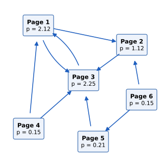
Figure 14.47. The six-page network of Exercise 14.22 with its PageRanks for \(d=0.85\). Code: fig_14_47. Reproduces Hastie, Tibshirani and Friedman (2009), Figure 14.47, with the computed PageRanks added. Download: PDF · SVG▶ DemoPageRank of the six-page web (Exercise 14.22)Compare the power method with the visit frequencies of a random surfer.Exercise 14.23 (an algorithm for NMF; Wu and Lange, 2007). A function \(g(x,y)\) minorises \(f(x)\) if
\[ g(x,y)\le f(x),\qquad g(x,x)=f(x) \tag{14.119} \]for all \(x,y\); then \(f\) is non-decreasing under
\[ x^{s+1}=\argmax_xg(x,x^s). \tag{14.120} \](a) Using the concavity of \(\log\), show that \(\log\sum_ky_k\ge\sum_kc_k\log(y_k/c_k)\) for \(y_k\ge0\), \(c_k\ge0\), \(\sum c_k=1\), and hence
\[ \log\sum_kw_{ik}h_{kj}\ge\sum_k\frac{a^s_{ikj}}{b^s_{ij}}\log\big(\frac{b^s_{ij}}{a^s_{ikj}}w_{ik}h_{kj}\big) \]with \(a^s_{ikj}=w^s_{ik}h^s_{kj}\), \(b^s_{ij}=\sum_kw^s_{ik}h^s_{kj}\). (b) Show that, up to constants,
\[ g(\bW,\bH\given\bW^s,\bH^s)=\sum_{i,j,k}x_{ij}\frac{a^s_{ikj}}{b^s_{ij}}(\log w_{ik}+\log h_{kj})-\sum_{i,j,k}w_{ik}h_{kj} \]minorises \(L(\bW,\bH)\). (c) Set its derivatives to zero to derive (14.74).
Solution
All three parts are in the proof of Result 14.22. (a) is Jensen's inequality \(\log\sum_kc_k(y_k/c_k)\ge\sum_kc_k\log(y_k/c_k)\) (terms with \(c_k=0\) are omitted), applied with \(c_k=a^s_{ikj}/b^s_{ij}\); equality holds when \(y_k/c_k\) does not depend on \(k\), in particular at \((\bW^s,\bH^s)\). (b) Multiply by \(x_{ij}\ge0\), sum, and subtract \(\sum(\bW\bH)_{ij}=\sum_{i,j,k}w_{ik}h_{kj}\) (exact); the dropped terms \(-\sum x_{ij}\frac{a}{b}\log\frac ab\) are constants. (The book prints \(u_{ij}\) in this display; it should be \(x_{ij}\).) (c)
\[ \partial g/\partial w_{ik}=\sum_jx_{ij}a^s_{ikj}/(b^s_{ij}w_{ik})-\sum_jh_{kj}=0 \]gives the first update of (14.74) with \(\bH=\bH^s\); similarly for \(h_{kj}\). On the 2s with \(r=10\), \(L\) increases at every one of 100 sweeps (smallest increase 2.92).
Exercise 14.24. For NMF with \(r=1\): (a) show that (14.74) becomes
\[ w_i\leftarrow w_i\frac{\sum_{j=1}^px_{ij}}{\sum_{j=1}^pw_ih_j},\qquad h_j\leftarrow h_j\frac{\sum_{i=1}^Nx_{ij}}{\sum_{i=1}^Nw_ih_j}, \tag{14.121} \]an iterative proportional scaling for the independence model of a two-way table; (b) show that the final iterates have the explicit form (the book's version)
\[ w_i=c\cdot\frac{\sum_{j=1}^px_{ij}}{\sum_{i=1}^N\sum_{j=1}^px_{ij}},\qquad h_k=\frac1c\cdot\frac{\sum_{i=1}^Nx_{ik}}{\sum_{i=1}^N\sum_{j=1}^px_{ij}}, \tag{14.122} \]for any \(c>0\), equivalent to the usual row and column estimates of the independence model.
Solution
(a) With \(r=1\), \((\bW\bH)_{ij}=w_ih_j\), and (14.74) gives
\[ w_i\leftarrow w_i\sum_jh_jx_{ij}/(w_ih_j)\big/\sum_jh_j=\sum_jx_{ij}/\sum_jh_j, \]which is (14.121); likewise for \(h_j\). Each step rescales the fitted row (column) totals to match the observed ones: \(\sum_jw_ih_j=\sum_jx_{ij}\) after the \(w\) step and \(\sum_iw_ih_j=\sum_ix_{ij}\) after the \(h\) step, which is iterative proportional scaling.
(b) Write \(x_{i+},x_{+j},x_{++}\) for the row, column and grand totals. From any positive start, the first \(w\) step gives \(w_i=x_{i+}/h_+\) (\(h_+\) the current column-parameter total), so \(w_+=x_{++}/h_+\); the \(h\) step then gives \(h_j=x_{+j}/w_+=x_{+j}h_+/x_{++}\). Hence after one sweep \(w_ih_j=x_{i+}x_{+j}/x_{++}\), the maximum likelihood fit of the independence model, and later sweeps leave it unchanged (we check this to \(10^{-15}\)). The final iterates are \(w_i=c\,x_{i+}/x_{++}\) and \(h_j=x_{+j}/c\) for some \(c>0\).
Note on the book: a factor \(x_{++}\) is missing in (14.122)
With (14.122) as printed, \(w_ih_k=x_{i+}x_{+k}/x_{++}^2\), which is the fit divided by the grand total \(x_{++}\); the fitted table would sum to 1 instead of \(x_{++}\). The second formula should read \(h_k=\frac1c\sum_ix_{ik}\) (or the first should have no denominator).
Exercise 14.25. Fit NMF with 25 basis elements to the 2s of the digits data, compare with a 24-component (plus mean) PCA model, and display \(\bW\) and \(\bH\) as in Figure 14.33.
Solution
Figure 14.33 above displays the factorisations (with uncentred rank-25 PCA so that all three read \(\bX\approx\bW\bH\)). For the requested comparison on the 731 training 2s in \([0,2]\): NMF with \(r=25\) (500 sweeps) leaves a residual sum of squares of 32,096, PCA with the mean and 24 components 19,879 (total centred sum of squares 84,036). PCA wins on squared error, as it must (it is the optimal rank-25 affine approximation, Result 14.13), and NMF optimises a Poisson likelihood rather than squared error. What NMF offers is the representation: its 25 basis images are localised strokes, combined with non-negative weights, while PCA's are global signed patterns that cancel. The NMF demonstration repeats this on 300 of the 2s for any rank.
Demonstrations for this chapter
Each demonstration runs in the browser and links back to these notes. The ▶ Demo boxes above open them already set to the case under discussion.
| Demonstration | What you can see | Sections and results |
|---|---|---|
| Spectral clustering and the graph Laplacian | The rings of Figure 14.29 with the nearest-neighbour graph, the smallest eigenvalues and eigenvectors of the Laplacian, the spectral embedding and the clustering, against K-means on the raw data; the number of neighbours, the kernel scale, the noise and the normalisation can be changed. Presets: 1 Figure 14.29; 2 K-means; 3 too few neighbours; 4 the fully connected graph; 5 two rings, random-walk Laplacian. | 14.5.3, 14.5.4; Results 14.17, 14.18 |
| PageRank and the damped random walk | The power method on the webs of Figures 14.46 and 14.47 and two others, with the damping \(d\), the iteration count, the start, and a random surfer whose visit frequencies estimate the PageRanks; the error against the rate \(d^k\). Presets: 1 Figure 14.46; 2 Figure 14.47; 3 a bad start; 4 \(d=1\) on two webs; 5 a dangling page. | 14.10; Result 14.28, Exercise 14.22 |
| Non-negative matrix factorisation of digits | NMF by the multiplicative updates on 300 handwritten 2s next to PCA: basis images, the reconstruction and weights of any digit, the log-likelihood along the sweeps, the squared errors. Presets: 1 \(r=25\); 2 the random start; 3 \(r=10\); 4 \(r=5\); 5 rank one. | 14.6; Result 14.22, Exercises 14.24–14.25 |
Related demonstrations in the companion courses: the K-means and EM demo and the kernel PCA demo (Bayesian and Probabilistic Machine Learning); the K-means quantisation, eigen-digits and ICA unmixing demos (Foundations of Deep Learning); the k-means and PAM, hierarchical clustering, choosing k and MDS demos (Statistical Methods for Modern Biology). The Python code for every figure of this page is in code/ch14_unsupervised_learning_a.py (Sections 14.2–14.5.1) and code/ch14_unsupervised_learning_b.py (Sections 14.5.2–14.10); see the code index.
References
- Hastie, T., Tibshirani, R. and Friedman, J. (2009). The Elements of Statistical Learning: Data Mining, Inference, and Prediction, 2nd edition. Springer, New York. Chapter 14, pp. 485–586. hastie.su.domains/ElemStatLearn.
- Agrawal, R., Mannila, H., Srikant, R., Toivonen, H. and Verkamo, A. I. (1995). Fast discovery of association rules. In Advances in Knowledge Discovery and Data Mining, AAAI/MIT Press.
- Bach, F. and Jordan, M. (2002). Kernel independent component analysis. Journal of Machine Learning Research, 3, 1–48.
- Brémaud, P. (1999). Markov Chains: Gibbs Fields, Monte Carlo Simulation, and Queues. Springer, New York.
- Chen, L. and Buja, A. (2008). Local multidimensional scaling for nonlinear dimension reduction, graph drawing and proximity analysis. Journal of the American Statistical Association, 104, 209–219.
- Cutler, A. and Breiman, L. (1994). Archetypal analysis. Technometrics, 36(4), 338–347.
- Donoho, D. and Stodden, V. (2004). When does non-negative matrix factorization give a correct decomposition into parts? In Advances in Neural Information Processing Systems 16, MIT Press.
- Duchamp, T. and Stuetzle, W. (1996). Extremal properties of principal curves in the plane. The Annals of Statistics, 24, 1511–1520.
- Eckart, C. and Young, G. (1936). The approximation of one matrix by another of lower rank. Psychometrika, 1, 211–218.
- Friedman, J. (1987). Exploratory projection pursuit. Journal of the American Statistical Association, 82, 249–266.
- Friedman, J. and Tukey, J. (1974). A projection pursuit algorithm for exploratory data analysis. IEEE Transactions on Computers, C-23, 881–889.
- Gersho, A. and Gray, R. (1992). Vector Quantization and Signal Compression. Kluwer, Boston.
- Hartigan, J. A. and Wong, M. A. (1979). Algorithm AS 136: a K-means clustering algorithm. Applied Statistics, 28, 100–108.
- Hastie, T. (1984). Principal Curves and Surfaces. PhD thesis, Stanford University.
- Hastie, T. and Stuetzle, W. (1989). Principal curves. Journal of the American Statistical Association, 84, 502–516.
- Hastie, T. and Tibshirani, R. (2003). Independent components analysis through product density estimation. In Advances in Neural Information Processing Systems 15, MIT Press.
- Hyvärinen, A., Karhunen, J. and Oja, E. (2001). Independent Component Analysis. Wiley, New York.
- Hyvärinen, A. and Oja, E. (2000). Independent component analysis: algorithms and applications. Neural Networks, 13, 411–430.
- Jolliffe, I. T., Trendafilov, N. T. and Uddin, M. (2003). A modified principal component technique based on the lasso. Journal of Computational and Graphical Statistics, 12, 531–547.
- Kaufman, L. and Rousseeuw, P. (1990). Finding Groups in Data: An Introduction to Cluster Analysis. Wiley, New York.
- Kohonen, T. (1990). The self-organizing map. Proceedings of the IEEE, 78, 1464–1479.
- Kohonen, T., Kaski, S., Lagus, K., Salojärvi, J., Paatero, A. and Saarela, A. (2000). Self organization of a massive document collection. IEEE Transactions on Neural Networks, 11(3), 574–585.
- Lee, D. D. and Seung, H. S. (1999). Learning the parts of objects by non-negative matrix factorization. Nature, 401, 788–791.
- Lee, D. D. and Seung, H. S. (2001). Algorithms for non-negative matrix factorization. In Advances in Neural Information Processing Systems 13, MIT Press.
- Lloyd, S. (1957, published 1982). Least squares quantization in PCM. IEEE Transactions on Information Theory, 28, 129–137.
- Macnaughton-Smith, P., Williams, W., Dale, M. and Mockett, L. (1964). Dissimilarity analysis: a new technique of hierarchical subdivision. Nature, 202, 1034–1035.
- MacQueen, J. (1967). Some methods for classification and analysis of multivariate observations. In Proceedings of the Fifth Berkeley Symposium on Mathematical Statistics and Probability, 1, 281–297.
- Mardia, K., Kent, J. and Bibby, J. (1979). Multivariate Analysis. Academic Press, London.
- Onton, J. and Makeig, S. (2006). Information-based modeling of event-related brain dynamics. Progress in Brain Research, 159, 99–120.
- Page, L., Brin, S., Motwani, R. and Winograd, T. (1998). The PageRank citation ranking: bringing order to the web. Technical report, Stanford Digital Library Technologies Project.
- Roweis, S. T. and Saul, L. K. (2000). Nonlinear dimensionality reduction by locally linear embedding. Science, 290, 2323–2326.
- Schölkopf, B., Smola, A. and Müller, K.-R. (1999). Kernel principal component analysis. In Advances in Kernel Methods: Support Vector Learning, MIT Press, 327–352.
- Silverman, B. (1986). Density Estimation for Statistics and Data Analysis. Chapman and Hall, London.
- Sjöstrand, K., Rostrup, E., Ryberg, C., Larsen, R., Studholme, C., Baezner, H., Ferro, J., Fazekas, F., Pantoni, L., Inzitari, D. and Waldemar, G. (2007). Sparse decomposition and modeling of anatomical shape variation. IEEE Transactions on Medical Imaging, 26(12), 1625–1635.
- Tarpey, T. and Flury, B. (1996). Self-consistency: a fundamental concept in statistics. Statistical Science, 11, 229–243.
- Tenenbaum, J. B., de Silva, V. and Langford, J. C. (2000). A global geometric framework for nonlinear dimensionality reduction. Science, 290, 2319–2323.
- Tibshirani, R., Walther, G. and Hastie, T. (2001). Estimating the number of clusters in a data set via the gap statistic. Journal of the Royal Statistical Society, Series B, 63(2), 411–423.
- von Luxburg, U. (2007). A tutorial on spectral clustering. Statistics and Computing, 17(4), 395–416.
- Wu, T. and Lange, K. (2007). The MM alternative to EM. Technical report, University of California, Los Angeles.
- Zou, H., Hastie, T. and Tibshirani, R. (2006). Sparse principal component analysis. Journal of Computational and Graphical Statistics, 15(2), 265–286.
The numerical statements in the text (the Apriori search against brute force, the dissimilarity identities, the descent properties of K-means, K-medoids, EM, the SOM, Procrustes averaging and the NMF updates, the agreement of our hierarchical clustering, kernel PCA, sparse PCA, FastICA, LLE and Isomap with library implementations, the Laplacian's zero eigenspace, the moment conditions of ProDenICA, the PageRank values and convergence rate, the exercises' identities, and the corrections in the notes on the book) were confirmed numerically.