Structured Distributions
A classifier's output distribution \(p(t\given\bx,\bw)\) is simple even when the network is not. Many deep learning models, though, are joint distributions over many variables with a rich structure: language models, normalising flows, variational autoencoders, diffusion models. This chapter introduces the language for that structure. A directed graph says how a joint distribution factorises into conditionals (Section 11.1); the same graph says which conditional independences every such distribution has, and they can be read off by d-separation (Section 11.2); and sequences are modelled by autoregressive factorisations, Markov chains and latent-variable state-space models (Section 11.3).
Ch. 1 Deep learning revolution Ch. 2 Probabilities Ch. 3 Standard distributions Ch. 4 Regression Ch. 5 Classification Ch. 6 Deep neural networks Ch. 7 Gradient descent Ch. 8 Backpropagation Ch. 9 Regularization Ch. 10 Convolutional networks Ch. 11 Structured distributions Ch. 12 Transformers Ch. 13 Graph neural networks Ch. 14 Sampling Ch. 15 Discrete latent variables Ch. 16 Continuous latent variables Ch. 17 GANs Ch. 18 Normalizing flows Ch. 19 Autoencoders Ch. 20 Diffusion models Appendices A to C
How to read these notes
They follow the book. Sections carry the book's numbers (11.1, 11.2.3, ...) and every displayed equation that appears in the book carries the book's own equation number, e.g. (11.13), so the notes can be read next to the book. Equations without a number are steps that the book skips.
Filling the gaps. Wherever the book states a result without proof, says it "can be shown" or "is easy to verify", or leaves it to an exercise, an orange Filling the gap box or a proof gives the full argument. Proofs and derivations start hidden: open one with its bar, or use the button below. Every numerical claim in them was confirmed by direct computation, mostly by enumerating joint probability tables exactly.
Figures and demonstrations. Only one figure of the chapter (11.23) is computed from a model; the others are graph diagrams. The diagrams that carry an argument are redrawn by the Python code with the statements they illustrate computed (the d-separation verdicts, the blocking nodes, the Markov blanket, the posterior probabilities), and five supplementary figures (11.S1 to 11.S5, our own) illustrate the gaps that are filled. The ▶ Demo boxes open an interactive demonstration already set to the case being discussed.
Main reference
C. M. Bishop and H. Bishop, Deep Learning: Foundations and Concepts, Springer (2024), Chapter 11, pages 325–356. Section, equation, figure and exercise numbers below refer to this book. The official solutions manual stops at Chapter 10, so every exercise solution here is my own. Further reading is listed in the references; the book's website is www.bishopbook.com.
The explanations, derivations, figures and code are my own; equations are cited by their numbers in the book.
Companion course: Bayesian and Probabilistic Machine Learning
Most of this chapter condenses Chapter 8 (graphical models) and part of Chapter 13 (sequential data) of the companion course Bayesian and Probabilistic Machine Learning (Bishop 2006). Where the full proof is already there, these notes give the statement and a short argument and link it; results that this book states differently get the full treatment here.
- Bayesian networks, the factorisation and acyclicity: Section 8.1, Result 8.1, Result 8.2 (here 11.1.2).
- Discrete variables, parameter counts, tied and logistic tables: Section 8.1.3, Result 8.4, Filling the gap 8.4 (here 11.1.3).
- Linear-Gaussian models: Section 8.1.4, Result 8.5 (here 11.1.4).
- Generative models and ancestral sampling: Section 8.1.2, Result 8.3 (here 11.2.5).
- Conditional independence, the three graphs, explaining away: Section 8.2.1, Result 8.7, Result 8.8, Filling the gap 8.6 (here 11.2.1–11.2.2).
- D-separation and its theorem, naive Bayes, the Markov blanket: Section 8.2.2, Result 8.9, Filling the gap 8.7, Result 8.10 (here 11.2.3–11.2.7). Undirected graphs and message passing, which this book only mentions: Section 8.3 and Section 8.4.
- Markov models, hidden Markov models and linear dynamical systems: Section 13.1, Result 13.3, Result 13.4, Section 13.2, Section 13.3 (here 11.3); autoregressive deep generative models: Advanced topics, Lecture 3.
- Demonstrations: d-separation, belief propagation, hidden Markov models, the Kalman filter, autoregressive images.
The chapter at a glance
- 11.1 A directed acyclic graph defines the product of conditionals (11.6); it is always normalised and its factors are the joint's own conditionals (Result 11.1). Leaving out links cuts the number of parameters from exponential to linear (Result 11.3). In a linear-Gaussian graph the joint is Gaussian with explicit mean, covariance and precision; the recursion (11.13) needs a restriction the book omits, and a missing link is a zero of the precision, not of the covariance (Results 11.4–11.6).
- 11.2 Conditional independence. Tail-to-tail and head-to-tail nodes block a path when observed; a head-to-head node blocks it unless it or a descendant is observed (Results 11.8, 11.9). Explaining away, with exact numbers and the reason in one likelihood ratio (Filling the gap 11.6). The d-separation theorem (Result 11.10) and the algorithm that decides it (Algorithm 11.1); naive Bayes fitted by maximum likelihood (Result 11.11); the Markov blanket (Result 11.13); and why the two "filters" pass the same distributions (Result 11.14).
- 11.3 Any sequence distribution is autoregressive (11.42); Markov chains of order \(M\) keep the last \(M\) values and have \(K^M(K-1)\) parameters (the book prints \(K^{M-1}(K-1)\)); maximum likelihood is counting, and on real text the held-out loss is best at an intermediate order (Results 11.16, 11.17, Figure 11.S4). A chain of latent states makes the observations depend on the whole past (Result 11.18), and the forward recursion that computes predictions is a recurrent network (Filling the gap 11.9).
Notation. \(\pa_k\) (or \(\pa(k)\)) is the set of parents of node \(k\), \(\ch_k\) its children, \(\an(S)\) the ancestors of a set \(S\). Nodes are numbered so that parents come before children (a topological order). \(a\indep b\given c\) means "\(a\) is conditionally independent of \(b\) given \(c\)", \(\emptyset\) the empty conditioning set. \(K\) is the number of states of a discrete variable; \(\bW\) collects the link weights \(w_{ij}\) of a linear-Gaussian graph, \(\bV=\diag(v_1,\dots,v_D)\) its noise variances. \(I(a;b\given c)\) is the conditional mutual information, zero exactly when \(a\indep b\given c\) (Section 2.5.7).
Printings. The first printing has a few slips in this chapter: a wrong exponent in the parameter count of an order-\(M\) Markov chain, a missing condition on the covariance recursion (11.13), a noise variance in a classifier that has none, and a mislabelled parameter in Exercise 11.5. Each is flagged with an Erratum note where it occurs; the list with the evidence is in Corrections to the book.
pp. 325–326 A network for binary classification defines the conditional distribution
\[ p(t\given\bx,\bw)=y(\bx,\bw)^t\{1-y(\bx,\bw)\}^{1-t}, \tag{11.1} \]whose negative log is the cross-entropy error of Section 5.4.3. However complicated \(y(\bx,\bw)\) is, (11.1) is a distribution over a single binary variable. The models of the later chapters are distributions over many variables at once, and probabilistic graphical models describe how such a joint distribution is built from simple pieces. Combined with neural networks that supply the pieces, they give models that are still trained end to end by stochastic gradient descent with automatic differentiation.
11.1 Graphical Models
See also the companion course, Section 8.1 (Bayesian networks).
p. 326 Every probabilistic computation in this book is a repeated use of the sum rule and the product rule (Section 2.1.2). Graphs add three things: a picture of a model's structure that helps in designing it, conditional independences that can be read off the picture, and a way to organise inference as local computations ("message passing") on the graph. The book draws neural networks in blue and graphical models in red; in a graphical model a node is a random variable and a link a probabilistic dependence, not a weighted connection.
11.1.1 Directed graphs
pp. 326–327 A graph has nodes (vertices) joined by links (edges). In a directed graphical model, also called a Bayesian network, the links are arrows. The other main class, Markov random fields or undirected graphical models, has links without direction; directed graphs suit causal, generative relationships and undirected graphs suit soft constraints between variables, and both are special cases of factor graphs (see Section 8.3 and Section 8.4.3 of the companion course). This chapter uses only directed graphs. Undirected graphs reappear in Chapter 13 of the book, as the graphs that graph neural networks act on, but there the nodes carry deterministic vectors, not random variables.
11.1.2 Factorization
pp. 327–328 For any joint distribution of three variables, two uses of the product rule give
\[ p(a,b,c)=p(c\given a,b)\,p(a,b), \tag{11.2} \] \[ p(a,b,c)=p(c\given a,b)\,p(b\given a)\,p(a). \tag{11.3} \]Draw one node per variable and an arrow into each node from every variable its factor is conditioned on: arrows \(a\to b\), \(a\to c\), \(b\to c\) (Figure 11.1). If there is an arrow from \(a\) to \(b\), \(a\) is a parent of \(b\) and \(b\) a child of \(a\). The left side of (11.3) is symmetric in \(a,b,c\) and the right side is not: another ordering gives another factorisation and another graph, all equally valid. For \(K\) variables the same argument gives the chain rule
\[ p(x_1,\dots,x_K)=p(x_K\given x_1,\dots,x_{K-1})\cdots p(x_2\given x_1)\,p(x_1), \tag{11.4} \]a fully connected graph in which every node receives an arrow from every lower-numbered node. It describes every distribution, so it says nothing. Information is in the missing links. The graph of Figure 11.2 has seven nodes and only eight links; reading off each node's parents gives
\[ p(x_1)p(x_2)p(x_3)p(x_4\given x_1,x_2,x_3)p(x_5\given x_1,x_3)p(x_6\given x_4)p(x_7\given x_4,x_5). \tag{11.5} \]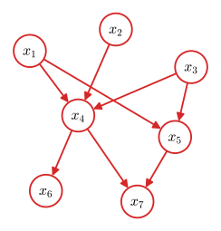
Definition 11.1 (directed acyclic graph; the factorisation it defines) pp. 328–329, (11.6)
A directed graph is acyclic (a DAG) if no directed path (a sequence of arrows followed in their direction) returns to its starting node. A distribution over \(\bx=(x_1,\dots,x_K)\) factorises over the DAG \(G\) if there are normalised conditional distributions \(f_k(x_k\given\pa_k)\), one per node, with
\[ p(x_1,\dots,x_K)=\prod_{k=1}^{K}p(x_k\given\pa_k). \tag{11.6} \]Nodes may stand for scalars, vectors or tensors, discrete or continuous; for continuous variables "distribution" means density and sums below become integrals. The set of all distributions that factorise over \(G\) is written \(\DF\) (Section 11.2.7).
The book states two properties without proof: the product (11.6) is normalised (Exercise 11.1), and acyclicity is the same as the existence of an ordering with all arrows pointing forward (Exercise 11.2). Both are needed for (11.6) to make sense, and there is a third, stronger fact behind the notation \(p(x_k\given\pa_k)\): the factors are not just some functions, they are the joint distribution's own conditionals.
Result 11.1 (the product (11.6) is a distribution, and its factors are its conditionals) p. 329; Exercise 11.1
Let the nodes be numbered in a topological order (parents before children) and let each \(f_k(\cdot\given\pa_k)\) be a normalised distribution for every value of its parents. Then \(p(\bx)=\prod_kf_k(x_k\given\pa_k)\) satisfies:
- \(p\ge0\) and \(\sum_{\bx}p(\bx)=1\);
- the marginal of the first \(k\) variables is \(p(x_1,\dots,x_k)=\prod_{j\le k}f_j(x_j\given\pa_j)\);
- the factors are the conditionals of \(p\): \[p(x_k\given x_1,\dots,x_{k-1})=p(x_k\given\pa_k)=f_k(x_k\given\pa_k).\]
Proof
(2) Fix \(k\) and sum over \(x_K\) first. Because \(K\) is last in the order, \(x_K\) is nobody's parent, so it appears only in \(f_K\), and \(\sum_{x_K}f_K(x_K\given\pa_K)=1\) whatever the values of \(\pa_K\). What remains is \(\prod_{j\le K-1}f_j\), the same expression with one node fewer, whose last node again appears only in its own factor. Repeating down to \(k+1\) gives (2).
(1) Non-negativity is clear; (2) with \(k=0\) (summing out every variable) gives total mass 1. This is Exercise 11.1.
(3) Divide (2) for \(k\) by (2) for \(k-1\): \[p(x_k\given x_1,\dots,x_{k-1})=\frac{\prod_{j\le k}f_j}{\prod_{j\le k-1}f_j}=f_k(x_k\given\pa_k).\] The right side depends on \(x_1,\dots,x_{k-1}\) only through \(\pa_k\subseteq\{x_1,\dots,x_{k-1}\}\). If a conditional distribution given a set of variables depends only on a subset \(S\) of them, it equals the conditional given \(S\); with \(S=\pa_k\), \[p(x_k\given\pa_k)=\E\big[p(x_k\given x_1,\dots,x_{k-1})\given\pa_k\big]=f_k(x_k\given\pa_k).\] So \(f_k=p(x_k\given\pa_k)\), which justifies writing the factors as \(p(x_k\given\pa_k)\). ∎
A direct computation confirms (1) and (3) on 20 random networks with two- and three-state nodes: the joint sums to 1 and every table equals the conditional computed from the joint.
Result 11.2 (acyclic means orderable) p. 329; Exercise 11.2
A finite directed graph has no directed cycle if and only if its nodes can be numbered so that every link goes from a lower to a higher number.
Proof
(\(\Leftarrow\), Exercise 11.2) Along a directed path the numbers strictly increase, so a path can never return to the node it started from.
(\(\Rightarrow\)) A finite DAG has a node with no parents: otherwise start anywhere and step to a parent repeatedly; after more steps than there are nodes some node repeats, and the repeated stretch, read forwards, is a directed cycle. Give such a node the number 1 and delete it with its links. The rest is still acyclic, so it has a parentless node, which gets number 2, and so on. Every link points from an earlier-deleted node to a later one, i.e. forward. (This is Kahn's algorithm, topological_order in the code; it agrees with an independent cycle test on 300 random graphs.) ∎
Filling the gap 11.1: "absence of links conveys information", precisely p. 328
The book says that the information in a graph is in its missing links. Here is the exact statement, which the rest of the chapter uses repeatedly.
Derivation
Claim (ordered Markov property). Number the nodes topologically. A distribution \(p\) factorises over \(G\) if and only if, for every \(k\), \[p(x_k\given x_1,\dots,x_{k-1})=p(x_k\given\pa_k),\quad\text{i.e.}\quad x_k\indep\{x_1,\dots,x_{k-1}\}\setminus\pa_k\given\pa_k .\]
(\(\Rightarrow\)) is part (3) of Result 11.1. (\(\Leftarrow\)) The chain rule (11.4) holds for every \(p\); replace each factor \(p(x_k\given x_1,\dots,x_{k-1})\) by \(p(x_k\given\pa_k)\) to obtain (11.6).
So deleting the link \(x_j\to x_k\) from the fully connected graph means exactly: \(x_k\) does not depend on \(x_j\) once its other predecessors are known. Each missing link removes one variable from one conditioning set of the chain rule. ∎
11.1.3 Discrete variables
See also the companion course, Section 8.1.3 and Result 8.4; the categorical distribution in Section 3.1.3 of this course.
pp. 329–331 A \(K\)-state variable in 1-of-\(K\) coding has
\[ p(\bx\given\bmu)=\prod_{k=1}^{K}\mu_k^{x_k}, \tag{11.7} \]with \(K-1\) free parameters because \(\sum_k\mu_k=1\). Two such variables have a joint table \(\mu_{kl}\) with \(K^2-1\) free entries, and \(M\) variables \(K^M-1\): exponential in \(M\). The graph decides where between "everything" and "independent" a model sits (Figures 11.3 to 11.5).
Result 11.3 (parameter counts for discrete graphs) pp. 330–332, Figures 11.3–11.6
If node \(k\) has \(K_k\) states, a general table \(p(x_k\given\pa_k)\) has \((K_k-1)\prod_{j\in\pa_k}K_j\) free parameters, and the graph has the sum of these. With all \(K_k=K\) and \(M\) nodes:
- fully connected: \(K^M-1\); no links: \(M(K-1)\);
- the chain of Figure 11.4: \(K-1+(M-1)K(K-1)\), linear in \(M\) and quadratic in \(K\);
- the chain with one transition table shared by all links (Figure 11.5): \(K-1+K(K-1)=K^2-1\), independent of \(M\);
- a binary child with \(M\) binary parents: \(2^M\) for a table, \(M+1\) for the logistic form
Proof
A table assigns a distribution over the \(K_k\) values of \(x_k\) (\(K_k-1\) free numbers) to each of the \(\prod_{j\in\pa_k}K_j\) parent configurations, independently. Summing over nodes gives the total.
(1) In the fully connected graph node \(k\) has \(k-1\) parents: \[\sum_{k=1}^{M}(K-1)K^{k-1}=(K-1)\frac{K^M-1}{K-1}=K^M-1,\] the same as the joint table, as it must be since (11.4) holds for every distribution. With no links each node contributes \(K-1\).
(2) The first node contributes \(K-1\) and each of the other \(M-1\) nodes, with one \(K\)-state parent, \(K(K-1)\).
(3) Tying the transition tables leaves one table of \(K(K-1)\) numbers plus the \(K-1\) of the first node.
(4) A binary child needs one number \(p(y=1\given\cdot)\) per parent configuration; (11.8) has the \(M+1\) weights \(w_0,\dots,w_M\). ∎
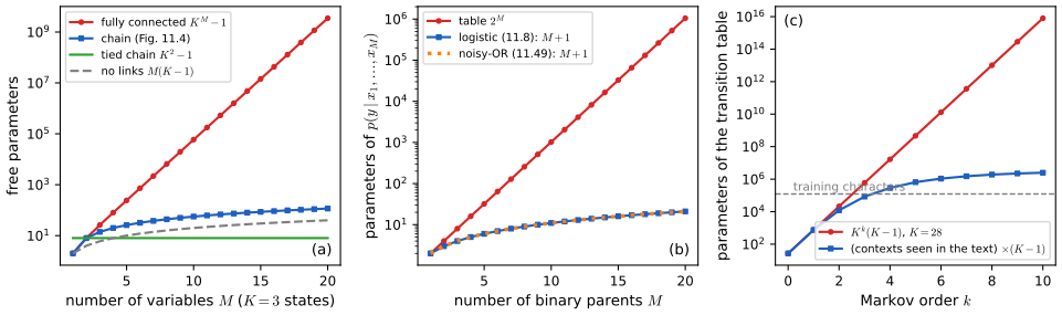
pp. 331–332 The logistic form (11.8) is to a table what a diagonal covariance is to a full one: a restricted family with a manageable number of parameters. The book does not say what is given up, nor how the noisy-OR of Exercise 11.5 compares.
Filling the gap 11.2: what the logistic table loses, and the noisy-OR as a latent-cause model pp. 331–332, (11.8); Exercise 11.5
Derivation
A table is a logistic model with all interactions. Write the log-odds of a general table as \(a(\bx)=\ln\frac{p(y=1\given\bx)}{p(y=0\given\bx)}\), one real number for each of the \(2^M\) parent configurations (when every probability is strictly between 0 and 1). Every function of \(M\) binary variables has a unique expansion \[a(\bx)=\sum_{S\subseteq\{1,\dots,M\}}\beta_S\prod_{i\in S}x_i,\] with \(\beta_S=\sum_{T\subseteq S}(-1)^{|S|-|T|}a(\mathbf{1}_T)\) (Möbius inversion: there are \(2^M\) coefficients for \(2^M\) values, and the system is triangular). The logistic model (11.8) keeps \(\beta_\emptyset=w_0\) and \(\beta_{\{i\}}=w_i\) and sets all interactions to zero. For two parents the lost term is \(\beta_{12}=a(1,1)-a(1,0)-a(0,1)+a(0,0)\): (11.8) cannot represent, for instance, "\(y\) is likely when exactly one parent is on".
The noisy-OR as a model with hidden inhibitors. Suppose each active cause \(x_i=1\) independently switches \(y\) on with probability \(\mu_i\), and an always-present "leak" does so with probability \(\mu_0\); \(y\) is on if any of them does. Then \(y=0\) requires every active cause and the leak to fail, so \[p(y=0\given\bx)=(1-\mu_0)\prod_{i=1}^{M}(1-\mu_i)^{x_i},\] which is (11.49). It also has \(M+1\) parameters, but it is linear on a different scale: \[\ln p(y=0\given\bx)=\ln(1-\mu_0)+\sum_ix_i\ln(1-\mu_i).\] Its log-odds do have interactions (the second cause adds less when the first is already on), so neither family contains the other. A direct computation verifies the formula against a simulation of the inhibitor story (\(2\times10^5\) draws per configuration, largest difference 0.0015). ∎
11.1.4 Gaussian variables
See also the companion course, Section 8.1.4 and Result 8.5; the linear-Gaussian model of two variables in Result 3.10 of this course.
pp. 332–333 In a linear-Gaussian model each node is Gaussian with a mean that is linear in its parents,
\[ p(x_i\given\pa(i))=\N\Big(x_i\,\Big|\sum_{j\in\pa(i)}w_{ij}x_j+b_i,\;v_i\Big), \tag{11.9} \]a family that contains probabilistic PCA, factor analysis and linear dynamical systems (Roweis and Ghahramani, 1999). The log of the joint is a sum over nodes,
\[ \ln p(\bx)=\sum_{i=1}^{D}\ln p(x_i\given\pa(i)) \tag{11.10} \] \[ =-\sum_{i=1}^{D}\frac{1}{2v_i}\Big(x_i-\sum_{j\in\pa(i)}w_{ij}x_j-b_i\Big)^2+\const, \tag{11.11} \]a quadratic in \(\bx\), so the joint is Gaussian. Its moments satisfy
\[ \E[x_i]=\sum_{j\in\pa(i)}w_{ij}\E[x_j]+b_i, \tag{11.12} \] \[ \cov[x_i,x_j]=\sum_{k\in\pa(j)}w_{jk}\cov[x_i,x_k]+I_{ij}v_j, \tag{11.13} \]which the book leaves to Exercises 11.6 and 11.7. Collect the weights in the matrix \(\bW\) (\(W_{ij}=w_{ij}\) if \(j\in\pa(i)\), else 0; strictly lower triangular in a topological numbering), the offsets in \(\bb\) and the variances in \(\bV=\diag(v_1,\dots,v_D)\).
Result 11.4 (a linear-Gaussian graph is a Gaussian, in closed form) p. 332, (11.9)–(11.11)
The joint distribution of (11.9) is \(\N(\bx\given\bmu,\Sig)\) with
\[ \bmu=(\bI-\bW)^{-1}\bb,\qquad \Sig=(\bI-\bW)^{-1}\bV(\bI-\bW)^{-\T},\qquad \Lam=\Sig^{-1}=(\bI-\bW)^\T\bV^{-1}(\bI-\bW). \]Proof
As a generative recipe. (11.9) says \(x_i=\sum_jw_{ij}x_j+b_i+\sqrt{v_i}\,\epsilon_i\) with independent \(\epsilon_i\sim\N(0,1)\), i.e. \(\bx=\bW\bx+\bb+\bV^{1/2}\beps\). Since \(\bW\) is strictly lower triangular, \(\bI-\bW\) is lower triangular with unit diagonal, so \(\det(\bI-\bW)=1\) and it is invertible: \[\bx=(\bI-\bW)^{-1}(\bb+\bV^{1/2}\beps).\] An affine function of a standard Gaussian vector is Gaussian with mean \((\bI-\bW)^{-1}\bb\) and covariance \((\bI-\bW)^{-1}\bV^{1/2}\bI\bV^{1/2}(\bI-\bW)^{-\T}\).
From (11.11). The bracket in (11.11) is the \(i\)th component of \((\bI-\bW)\bx-\bb\), so \[\ln p(\bx)=-\tfrac12\big((\bI-\bW)\bx-\bb\big)^\T\bV^{-1}\big((\bI-\bW)\bx-\bb\big)+\const,\] a Gaussian exponent with precision \(\Lam=(\bI-\bW)^\T\bV^{-1}(\bI-\bW)\) and mean solving \((\bI-\bW)\bmu=\bb\). The "const" is also right: the product of the \(D\) normalisers \((2\pi v_i)^{-1/2}\) equals \((2\pi)^{-D/2}|\Lam|^{1/2}\) because \(|\Lam|=\det(\bI-\bW)^2/\prod_iv_i=1/\prod_iv_i\). ∎
Result 11.5 (the recursions (11.12) and (11.13), and when (11.13) holds) pp. 332–333; Exercises 11.6, 11.7
- (11.12) holds for every \(i\); evaluated in topological order, each mean uses only means already computed.
- (11.13) holds whenever \(x_i\) is not a descendant of \(x_j\), in particular for all \(i\le j\) in a topological numbering. Evaluated column by column (\(j=1,2,\dots\), and \(i=1,\dots,j\) within a column), each entry uses only entries already computed; the entries with \(i>j\) follow from symmetry.
- For \(i\) a descendant of \(j\), (11.13) is false in general.
Erratum (p. 333): the book states (11.13) for all \(i,j\). Example: the two-node graph \(x_1\to x_2\). With \(i=2\), \(j=1\), (11.13) gives \(\cov[x_2,x_1]=0+I_{21}v_1=0\) since \(x_1\) has no parents, but in fact \(\cov[x_2,x_1]=w_{21}v_1\). The recursion is correct for the upper triangle, which is how the book then uses it ("starting from the lowest numbered node").
Proof (Exercises 11.6 and 11.7)
Take expectations in \(x_i=\sum_{j\in\pa(i)}w_{ij}x_j+b_i+\sqrt{v_i}\epsilon_i\) with \(\E[\epsilon_i]=0\): this is (11.12).
For the covariance, write node \(j\)'s equation and use bilinearity of \(\cov\): \[\cov[x_i,x_j]=\sum_{k\in\pa(j)}w_{jk}\cov[x_i,x_k]+\sqrt{v_j}\,\cov[x_i,\epsilon_j].\] Unrolling the recursion, \(x_i\) is a linear function of \(\epsilon_i\) and of the \(\epsilon_l\) of its ancestors only. If \(x_i\) is not a descendant of \(x_j\) and \(i\ne j\), then \(j\) is not among them, and \(\epsilon_j\) is independent of \(x_i\): \(\cov[x_i,\epsilon_j]=0\). If \(i=j\), then \(x_j=(\text{terms independent of }\epsilon_j)+\sqrt{v_j}\epsilon_j\), so \(\cov[x_j,\epsilon_j]=\sqrt{v_j}\). Together, \(\sqrt{v_j}\cov[x_i,\epsilon_j]=I_{ij}v_j\): this is (11.13). If \(x_i\) is a descendant of \(x_j\), \(\cov[x_i,\epsilon_j]\ne0\) in general and the term is missing, which gives the counterexample.
Order of evaluation: entry \((i,j)\) with \(i\le j\) needs \(\cov[x_i,x_k]\) for \(k\in\pa(j)\), so \(k<j\). If \(i\le k\) this is an entry of an earlier column; if \(k<i\) it equals \(\cov[x_k,x_i]\), an entry of column \(i\le j\) above the diagonal, computed earlier in this column or in an earlier one. ∎
A direct computation confirms both recursions against the closed form of Result 11.4 on a random six-node graph, and the counterexample.
p. 333 Two extremes. With no links there are \(D\) offsets and \(D\) variances: \(\bmu=\bb\), \(\Sig=\diag(v_1,\dots,v_D)\), \(2D\) parameters, \(D\) independent Gaussians. With every lower-numbered node a parent, the weights and variances together number \(D(D+1)/2\), exactly those of a general symmetric covariance (Exercise 11.8). The book stops at the count; the stronger statement is that every covariance is reached.
Result 11.6 (a fully connected linear-Gaussian graph is a general Gaussian) p. 333; Exercise 11.8
The fully connected graph has \(D(D-1)/2\) weights and \(D\) variances, \(D(D+1)/2\) in all. Every positive definite \(\Sig\) arises from exactly one choice: \(\bw_i=(w_{i1},\dots,w_{i,i-1})\) are the coefficients of the regression of \(x_i\) on \(x_1,\dots,x_{i-1}\), \(\bw_i=\Sig_{1:i-1,1:i-1}^{-1}\Sig_{1:i-1,i}\), and \(v_i=\Sigma_{ii}-\Sig_{i,1:i-1}\bw_i>0\) is the residual variance.
Proof
Counting: node \(i\) has \(i-1\) weights, \(\sum_{i=1}^{D}(i-1)=D(D-1)/2\), plus \(D\) variances. A symmetric \(D\times D\) matrix has \(D(D+1)/2\) free entries.
Reaching every \(\Sig\): the Cholesky factorisation gives a unique \(\Sig=\bL\bm D\bL^\T\) with \(\bL\) unit lower triangular and \(\bm D\) diagonal and positive. Put \(\bI-\bW=\bL^{-1}\) (unit lower triangular, so \(\bW\) is strictly lower triangular) and \(\bV=\bm D\); then Result 11.4 gives covariance \(\bL\bm D\bL^\T=\Sig\). The explicit formulas are the conditional mean and variance of a Gaussian (Result 3.7): \(x_i\given x_{1:i-1}\) has mean \(\mu_i+\bw_i^\T(\bx_{1:i-1}-\bmu_{1:i-1})\) and variance \(v_i\), a Schur complement of a positive definite matrix and so positive. A numerical experiment rebuilds a random \(5\times5\) covariance this way exactly. ∎
p. 333 In between, missing links constrain the covariance. For the chain \(x_1\to x_2\to x_3\) of Figure 11.7 (no link from \(x_1\) to \(x_3\)) the recursions give (Exercise 11.9)
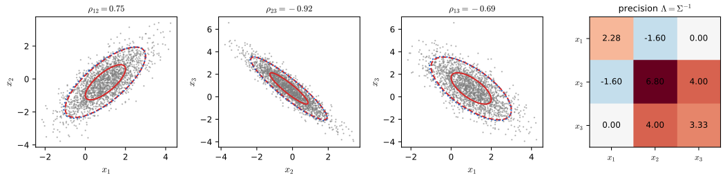
\[ \bmu=\big(b_1,\;b_2+w_{21}b_1,\;b_3+w_{32}b_2+w_{32}w_{21}b_1\big)^\T, \tag{11.14} \] \[ \Sig=\begin{pmatrix}v_1&w_{21}v_1&w_{32}w_{21}v_1\\ w_{21}v_1&v_2+w_{21}^2v_1&w_{32}(v_2+w_{21}^2v_1)\\ w_{32}w_{21}v_1&w_{32}(v_2+w_{21}^2v_1)&v_3+w_{32}^2(v_2+w_{21}^2v_1)\end{pmatrix}. \tag{11.15} \]Notice that \(\Sigma_{13}=w_{32}w_{21}v_1\ne0\): the missing link does not make \(x_1\) and \(x_3\) uncorrelated. Where does it show up, then?
Filling the gap 11.3: a missing link is a zero of the precision matrix p. 333, Figure 11.7
Derivation
Write \(\bm B=\bI-\bW\). By Result 11.4, \[\Lambda_{ij}=\sum_{k=1}^{D}\frac{B_{ki}B_{kj}}{v_k}.\] \(B_{ki}\ne0\) only if \(k=i\) or \(i\in\pa(k)\). For \(i\ne j\) a term is nonzero only if (a) \(k=i\) and \(j\in\pa(i)\), (b) \(k=j\) and \(i\in\pa(j)\), or (c) both \(i,j\in\pa(k)\). Hence \[\Lambda_{ij}=0\quad\text{unless } i,j \text{ are linked or share a child (are co-parents).}\] For a Gaussian, \(\Lambda_{ij}=0\) is equivalent to \(x_i\indep x_j\given\) (all the other variables): the conditional distribution of \((x_i,x_j)\) given the rest has precision equal to the \(2\times2\) block of \(\Lam\) (Result 3.7), which is diagonal exactly when \(\Lambda_{ij}=0\). The partial correlation given the rest is \(-\Lambda_{ij}/\sqrt{\Lambda_{ii}\Lambda_{jj}}\).
Figure 11.7. With \(w_{31}=0\), \[\Lambda_{13}=\frac{B_{11}B_{13}}{v_1}+\frac{B_{21}B_{23}}{v_2}+\frac{B_{31}B_{33}}{v_3}=0\] because \(B_{13}=B_{23}=0\) and \(B_{31}=-w_{31}=0\). So \(x_1\indep x_3\given x_2\), the head-to-tail independence of Section 11.2, while \(\Sigma_{13}\ne0\).
The collider \(x_1\to x_3\leftarrow x_2\) (\(w_{21}=0\)): now \(\Sigma_{12}=0\) (independent causes) but \(\Lambda_{12}=B_{31}B_{32}/v_3=w_{31}w_{32}/v_3\ne0\): given \(x_3\), the causes are dependent. This is explaining away for Gaussians. The zero pattern of \(\Lam\) is the "moral graph" (links plus married co-parents) of the companion course's Section 8.3.4; a direct computation finds all eight structural zeros of a random six-node graph. ∎
p. 333 The same construction works when each node is a vector,
\[ p(\bx_i\given\pa(i))=\N\Big(\bx_i\,\Big|\sum_{j\in\pa(i)}\bW_{ij}\bx_j+\bb_i,\;\Sig_i\Big), \tag{11.16} \]with matrices \(\bW_{ij}\), non-square when \(\bx_i\) and \(\bx_j\) differ in dimension.
Filling the gap 11.4: vector-valued nodes give a Gaussian, with block recursions p. 333, (11.16); Exercise 11.10
Derivation
Stack the nodes into \(\bx=(\bx_1,\dots,\bx_D)\) and the blocks \(\bW_{ij}\) into a block strictly lower triangular \(\bW\); let \(\bV=\mathrm{blockdiag}(\Sig_1,\dots,\Sig_D)\). Then \(\bx=\bW\bx+\bb+\bV^{1/2}\beps\) with \(\beps\sim\N(\bzero,\bI)\), \(\bI-\bW\) is block unit lower triangular (determinant 1), and the argument of Result 11.4 applies word for word: \(\bx\) is Gaussian with mean \((\bI-\bW)^{-1}\bb\) and covariance \((\bI-\bW)^{-1}\bV(\bI-\bW)^{-\T}\). The proof of Result 11.5 also carries over, with \(\cov[\bx_i,\bx_j]=\E[(\bx_i-\bmu_i)(\bx_j-\bmu_j)^\T]\): \[\bmu_i=\sum_{j\in\pa(i)}\bW_{ij}\bmu_j+\bb_i,\qquad \cov[\bx_i,\bx_j]=\sum_{k\in\pa(j)}\cov[\bx_i,\bx_k]\bW_{jk}^\T+I_{ij}\Sig_j\quad(\bx_i\text{ not a descendant of }\bx_j).\] A direct computation compares these block recursions with the stacked closed form for nodes of dimensions 2, 3 and 1. ∎
11.1.5 Binary classifier
p. 334 A two-class network classifier with a Gaussian prior on its weights (Section 2.6.2) is the joint distribution
\[ p(\bt,\bw\given\bX,\lambda)=p(\bw\given\lambda)\prod_{n=1}^{N}p(t_n\given\bw,\bx_n), \tag{11.17} \] \[ p(\bw\given\lambda)=\N(\bw\given\bzero,\lambda\bI), \tag{11.18} \]with \(p(t_n\given\bw,\bx_n)\) given by (11.1). Its random variables are \(t_1,\dots,t_N\) and \(\bw\): the graph is \(\bw\) with an arrow to each \(t_n\) (Figure 11.8). A plate, a box labelled \(N\) around one representative node \(t_n\), stands for the \(N\) copies (Figure 11.9). Note that in (11.18) \(\lambda\) is the prior variance (not a precision as elsewhere in the book).
Erratum (p. 334, Figures 11.10 and 11.11): the text says this model "contains the noise variance \(\sigma^2\)", and the figures draw a node \(\sigma^2\). The Bernoulli likelihood (11.1) has no noise variance; \(\sigma^2\) belongs to the regression version of the model, and the next page indeed speaks of "the linear regression model". For the classifier the only deterministic parameters are \(\lambda\) and the inputs \(\bx_n\) (Figure 11.12 correctly omits \(\sigma^2\)).
11.1.6 Parameters and observations
pp. 334–336 Conventions: random variables are open circles; deterministic quantities (parameters such as \(\lambda\), inputs \(\bx_n\)) are small floating symbols; an observed random variable, set to its value in the data, is shaded. An unobserved random variable such as \(\bw\) is a latent or hidden variable. For a new input \(\hat\bx\) the joint distribution of all random variables is
\[ p(\hat t,\bt,\bw\given\hat\bx,\bX,\lambda)=p(\bw\given\lambda)\,p(\hat t\given\bw,\hat\bx)\prod_{n=1}^{N}p(t_n\given\bw,\bx_n) \tag{11.19} \](Figure 11.12). The book describes the prediction in words; here it is from (11.19).
Filling the gap 11.5: the predictive distribution, read off (11.19) pp. 335–336
Derivation
By the sum and product rules applied to (11.19), with \(\bt\) observed, \[p(\hat t\given\hat\bx,\bt,\bX,\lambda)=\frac{\int p(\hat t,\bt,\bw\given\hat\bx,\bX,\lambda)\,\d\bw}{\sum_{\hat t}\int p(\hat t,\bt,\bw\given\hat\bx,\bX,\lambda)\,\d\bw}=\int p(\hat t\given\bw,\hat\bx)\,\underbrace{\frac{p(\bw\given\lambda)\prod_np(t_n\given\bw,\bx_n)}{\int p(\bw'\given\lambda)\prod_np(t_n\given\bw',\bx_n)\,\d\bw'}}_{p(\bw\given\bt,\bX,\lambda)}\,\d\bw,\] where the sum over \(\hat t\) of \(p(\hat t\given\bw,\hat\bx)\) is 1. So the prediction averages the network's output distribution over the posterior of the weights. Two facts make this possible: \(\hat t\) enters (11.19) only through \(p(\hat t\given\bw,\hat\bx)\), which is the conditional independence \(\hat t\indep t_n\given\bw\) of (11.36) below; and the posterior does not involve \(\hat\bx\).
The integral over millions of weights is intractable for deep networks, so the book replaces the posterior by a point mass at \(\bw_{\mathrm{MAP}}=\argmax_\bw p(\bw\given\bt,\bX,\lambda)\), giving \(p(\hat t\given\bw_{\mathrm{MAP}},\hat\bx)\). With the prior (11.18), \(-\ln p(\bw\given\bt,\bX,\lambda)\) is the cross-entropy error plus \(\|\bw\|^2/(2\lambda)\): MAP is weight decay (Section 2.6.2). ∎
11.1.7 Bayes' theorem
pp. 336–337 Observing variables changes the distribution of the others; computing the new distributions is inference. The simplest case is the two-node graph \(x\to y\), \(p(x,y)=p(x)p(y\given x)\), with \(y\) observed:
\[ p(y)=\sum_{x'}p(y\given x')p(x'), \tag{11.20} \] \[ p(x\given y)=\frac{p(y\given x)p(x)}{p(y)}. \tag{11.21} \]The joint is now written \(p(y)p(x\given y)\), the graph \(y\to x\) with the arrow reversed (Figure 11.13). Both graphs on two nodes are complete, so both describe every joint distribution and the reversal loses nothing; a direct computation confirms that the reversed tables give the same joint. For larger graphs, inference can exploit the graph by passing local messages: exact on trees, approximate (loopy belief propagation) on graphs with cycles. This book does not develop it; see the companion course's Section 8.4 and its belief propagation demo.
11.2 Conditional Independence
See also the companion course, Section 8.2 and Result 8.6.
Definition 11.2 (conditional independence; Dawid, 1979, 1980) p. 337, (11.22)–(11.24)
\(a\) is conditionally independent of \(b\) given \(c\) if
\[ p(a\given b,c)=p(a\given c), \tag{11.22} \]for every value of \(b\) and \(c\) with \(p(b,c)>0\); equivalently
\[ p(a,b\given c)=p(a\given b,c)p(b\given c)=p(a\given c)p(b\given c), \tag{11.23} \]for every \(c\) with \(p(c)>0\). It is written
\[ a\indep b\given c. \tag{11.24} \]\(a,b,c\) may be sets of variables; \(c=\emptyset\) is ordinary independence.
Result 11.7 (equivalent forms and three rules) p. 337; Exercise 11.11
- (11.22) \(\Leftrightarrow\) (11.23) \(\Leftrightarrow\) \(p(a,b,c)=f(a,c)\,g(b,c)\) for some functions \(f,g\) (factorisation criterion).
- Symmetry: \(a\indep b\given c\Rightarrow b\indep a\given c\).
- Decomposition (Exercise 11.11): \(a\indep(b,d)\given c\Rightarrow a\indep b\given c\).
- Weak union: \(a\indep(b,d)\given c\Rightarrow a\indep b\given(c,d)\).
Proof
(1) (11.22)\(\Rightarrow\)(11.23) is the displayed computation. (11.23)\(\Rightarrow\)(11.22): divide \(p(a,b\given c)=p(a\given c)p(b\given c)\) by \(p(b\given c)>0\). (11.23)\(\Rightarrow\) factorisation: \(p(a,b,c)=p(a\given c)\cdot p(b\given c)p(c)\). Factorisation \(\Rightarrow\)(11.23): summing \(f(a,c)g(b,c)\) gives \(p(a,c)=f(a,c)G(c)\), \(p(b,c)=F(c)g(b,c)\) and \(p(c)=F(c)G(c)\) with \(F(c)=\sum_af(a,c)\), \(G(c)=\sum_bg(b,c)\); so \[\frac{p(a,c)\,p(b,c)}{p(c)}=f(a,c)g(b,c)=p(a,b,c),\] which is (11.23) multiplied by \(p(c)\).
(2) (11.23) is symmetric in \(a\) and \(b\).
(3) Sum (11.23) for the pair \((a,(b,d))\), \(p(a,b,d\given c)=p(a\given c)p(b,d\given c)\), over \(d\): \(p(a,b\given c)=p(a\given c)p(b\given c)\).
(4) By (1), \(p(a,b,c,d)=f(a,c)g(b,d,c)\), which is also of the form \(f'(a,(c,d))\,g'(b,(c,d))\); apply (1) with conditioning set \((c,d)\). ∎
p. 338 Checking a conditional independence by algebra on the factorised joint is tedious. The point of the graph is that the independences implied by the factorisation can be read off it by d-separation (Pearl, 1988). The three graphs of Section 11.2.1 contain the whole idea.
11.2.1 Three example graphs
See also the companion course, Section 8.2.1 and Result 8.7.
pp. 338–341 The three graphs on \(a,b,c\) in which \(a\) and \(b\) are joined through \(c\) factorise as
\[ p(a,b,c)=p(a\given c)p(b\given c)p(c), \tag{11.25} \] \[ p(a,b)=\sum_cp(a\given c)p(b\given c)p(c), \tag{11.26} \] \[ p(a,b,c)=p(a)p(c\given a)p(b\given c), \tag{11.28} \] \[ p(a,b,c)=p(a)p(b)p(c\given a,b), \tag{11.30} \]the tail-to-tail graph \(a\leftarrow c\to b\) (Figure 11.14), the head-to-tail chain \(a\to c\to b\) (Figure 11.16) and the head-to-head graph \(a\to c\leftarrow b\) (Figure 11.18), where \(c\) is called a collider. The book shows that independence holds where it does; for "does not hold in general" it only says the expression "does not factorize". Here are both halves, with explicit measures of the dependence.
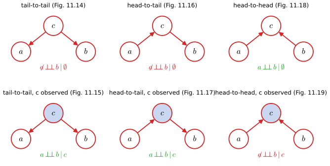
d_separated), green when \(a\indep b\) is implied and red when it is not. Observing \(c\) blocks the first two paths and opens the third. Redraws Bishop and Bishop (2024), Figures 11.14–11.19. Download: PDF · SVGResult 11.8 (the three three-node graphs) pp. 338–341, (11.25)–(11.31)
- Tail-to-tail (11.25): \(a\indep b\given c\) always; and \(a\nindep b\given\emptyset\) in general. For binary variables, with \(\alpha_c=p(a=1\given c)\), \(\beta_c=p(b=1\given c)\), \(\pi=p(c=1)\): \[\cov[a,b]=\pi(1-\pi)(\alpha_1-\alpha_0)(\beta_1-\beta_0).\]
- Head-to-tail (11.28): \(a\indep b\given c\) always; and \(a\nindep b\given\emptyset\) in general: with \(\gamma_a=p(c=1\given a)\), \(\beta_c=p(b=1\given c)\), \[\cov[a,b]=\var[a]\,(\gamma_1-\gamma_0)(\beta_1-\beta_0).\]
- Head-to-head (11.30): \(a\indep b\given\emptyset\) always; and \(a\nindep b\given c\) in general: for binary \(a,b\), \(a\indep b\given c=c_0\) holds if and only if \[p(c_0\given0,0)\,p(c_0\given1,1)=p(c_0\given0,1)\,p(c_0\given1,0).\]
So \(a\indep b\given c\) for the first two graphs and \(a\indep b\given\emptyset\) for the third hold for every choice of tables; the opposite statements fail except on a set of tables of measure zero (where a difference or the cross-ratio above happens to vanish).
Proof
(1) \(p(a,b\given c)=p(a,b,c)/p(c)=p(a\given c)p(b\given c)\). Marginally, \(\E[ab]=\E_c[\alpha_c\beta_c]\), \(\E[a]=\E_c[\alpha_c]\), \(\E[b]=\E_c[\beta_c]\), so \(\cov[a,b]=\cov_c[\alpha_c,\beta_c]\); for binary \(c\), \(\alpha_c=\alpha_0+(\alpha_1-\alpha_0)c\) and similarly \(\beta_c\), giving \((\alpha_1-\alpha_0)(\beta_1-\beta_0)\var[c]\). Nonzero covariance means dependence.
(2) By Bayes' theorem \(p(a)p(c\given a)/p(c)=p(a\given c)\), so \[p(a,b\given c)=\frac{p(a)p(c\given a)p(b\given c)}{p(c)}=p(a\given c)p(b\given c).\] Marginally \[p(b=1\given a)=\sum_cp(c\given a)\beta_c=\beta_0+(\beta_1-\beta_0)\gamma_a,\] so \[\cov[a,b]=\cov\big[a,p(b=1\given a)\big]=(\beta_1-\beta_0)\cov[a,\gamma_a]=(\beta_1-\beta_0)(\gamma_1-\gamma_0)\var[a].\]
(3) Summing (11.30) over \(c\) gives \(p(a,b)=p(a)p(b)\), which is (11.31). Given \(c=c_0\), \(p(a,b\given c_0)\propto q_{ab}=p(a)p(b)p(c_0\given a,b)\). A \(2\times2\) table is a product \(f(a)g(b)\) if and only if it has rank one, i.e. \(q_{00}q_{11}=q_{01}q_{10}\); the factors \(p(a)p(b)\) cancel from both sides, leaving the cross-ratio condition. For the fuel gauge below with \(c_0\) = "reads empty": \(0.9\times0.2=0.18\ne0.8\times0.8=0.64\), so battery and fuel are dependent given the reading.
A numerical experiment draws 30 random tables for each graph and confirms \(I(a;b\given c)=0\), \(I(a;b)>0\) for the first two and the reverse for the third. ∎
p. 341 In each case the graph explains the result: a path from \(a\) to \(b\) through a tail-to-tail or head-to-tail node carries dependence until that node is observed, which blocks it; a path through a head-to-head node is blocked until the node is observed, which unblocks it. One more case completes the picture: \(y\) is a descendant of \(x\) if a directed path leads from \(x\) to \(y\).
Result 11.9 (observing a descendant of a collider) p. 341; Exercise 11.13, Figure 11.32
In the graph \(a\to c\leftarrow b\), \(c\to d\) (Figure 11.32), \(a\indep b\given\emptyset\), but in general \(a\nindep b\given d\): a head-to-head path is unblocked when the collider or any of its descendants is observed.
Proof (Exercise 11.13)
\(p(a,b,c,d)=p(a)p(b)p(c\given a,b)p(d\given c)\). Summing over \(d\) and then \(c\) gives \(p(a,b)=p(a)p(b)\). Given \(d\), \[p(a,b\given d)\propto p(a)p(b)\sum_cp(c\given a,b)p(d\given c)=p(a)p(b)\,\tilde p(d\given a,b),\] where \(\tilde p(d\given a,b)=\sum_cp(d\given c)p(c\given a,b)\) is a conditional distribution of \(d\) given \(a,b\). This is the head-to-head case of Result 11.8(3) with \(d\) in the place of \(c\), so \(a\) and \(b\) are dependent given \(d\) unless the cross-ratio of \(\tilde p\) happens to equal 1. A noisy copy of the collider still carries information about how its parents combined. The driver of Exercise 11.14 below is a concrete case; a direct computation confirms \(I(a;b\given d)>0\) for 30 random tables. ∎
11.2.2 Explaining away
See also the companion course, Filling the gap 8.6 (the same fuel-gauge numbers).
pp. 341–343 A car has a battery \(B\) (1 charged, 0 flat), a fuel tank \(F\) (1 full, 0 empty) and an electric fuel gauge \(G\) (1 reads full, 0 reads empty) that depends on both (Figure 11.20). The book's numbers are \(p(B=1)=p(F=1)=0.9\) and
\(p(G=1\given B=1,F=1)=0.8\), \(p(G=1\given B=1,F=0)=0.2\), \(p(G=1\given B=0,F=1)=0.2\), \(p(G=1\given B=0,F=0)=0.1\)
(an unreliable gauge). Observing that the gauge reads empty,
\[ p(G=0)=\sum_{B\in\{0,1\}}\sum_{F\in\{0,1\}}p(G=0\given B,F)p(B)p(F)=0.315, \tag{11.32} \] \[ p(G=0\given F=0)=\sum_{B\in\{0,1\}}p(G=0\given B,F=0)p(B)=0.81, \tag{11.33} \] \[ p(F=0\given G=0)=\frac{p(G=0\given F=0)p(F=0)}{p(G=0)}\simeq0.257, \tag{11.34} \]up from the prior 0.1. Then the battery is found flat:
\[ p(F=0\given G=0,B=0)=\frac{p(G=0\given B=0,F=0)p(F=0)}{\sum_{F\in\{0,1\}}p(G=0\given B=0,F)p(F)}\simeq0.111. \tag{11.35} \]The flat battery explains away the empty reading.
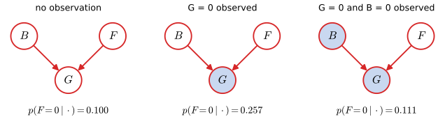
Filling the gap 11.6: the numbers exactly, and why the battery matters so much pp. 342–343, (11.32)–(11.35)
Derivation
The sums. \(p(G=0\given B,F)\) is \(0.9,0.8,0.8,0.2\) for \((B,F)=(0,0),(0,1),(1,0),(1,1)\), and \(p(B,F)=0.01,0.09,0.09,0.81\). So \[p(G=0)=0.009+0.072+0.072+0.162=0.315,\qquad p(G=0\given F=0)=0.9\cdot0.1+0.8\cdot0.9=0.81,\] \[p(F=0\given G=0)=\frac{0.81\times0.1}{0.315}=\frac{9}{35}=0.2571,\qquad p(F=0\given G=0,B=0)=\frac{0.9\times0.1}{0.9\times0.1+0.8\times0.9}=\frac{0.09}{0.81}=\frac19=0.1111.\] In (11.35) \(p(B=0)\) cancels because \(B\indep F\) a priori.
Why. In odds form, for a fixed battery state \(B\), \[\frac{p(F=0\given G=0,B)}{p(F=1\given G=0,B)}=\frac{p(G=0\given B,F=0)}{p(G=0\given B,F=1)}\times\frac{p(F=0)}{p(F=1)}.\] The likelihood ratio is \(0.8/0.2=4\) when the battery is charged but only \(0.9/0.8=1.125\) when it is flat: with a flat battery the gauge reads empty almost regardless of the fuel, so the reading says little about the tank. Not knowing \(B\), we average, and the reading counts for something in between. Conversely, learning that the battery is charged makes the reading more credible: \[p(F=0\given G=0,B=1)=\frac{0.8\cdot0.1}{0.8\cdot0.1+0.2\cdot0.9}=\frac{4}{13}=0.308>0.257.\] Either way, once \(G\) is known, learning \(B\) changes our belief about \(F\): they are dependent given \(G\), as Result 11.8(3) predicted.
The value 0.111 is still above the prior 0.1 because 1.125 > 1: even with a flat battery an empty reading is slightly more likely when the tank is empty. All four numbers are checked exactly (as fractions 9/35, 1/9, 4/13). ∎
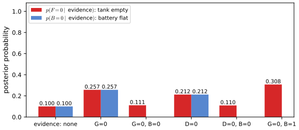
11.2.3 D-separation
See also the companion course, Section 8.2.2, Result 8.9 (the theorem with its proof) and the d-separation demo.
Definition 11.3 (blocked paths; d-separation; Pearl, 1988) p. 343
Let \(A,B,C\) be disjoint sets of nodes of a DAG. A path is a sequence of distinct nodes, each joined to the next by a link in either direction. A path from \(A\) to \(B\) is blocked by \(C\) if it contains a node at which
(a) the arrows meet head-to-tail or tail-to-tail, and the node is in \(C\); or
(b) the arrows meet head-to-head, and neither the node nor any of its descendants is in \(C\).
If every path from a node of \(A\) to a node of \(B\) is blocked, \(A\) is d-separated from \(B\) by \(C\).
Result 11.10 (the d-separation theorem; Pearl, 1988; Geiger, Verma and Pearl, 1990; Lauritzen, 1996) pp. 343, 348–349
- Soundness. If \(C\) d-separates \(A\) from \(B\) in \(G\), then \(A\indep B\given C\) for every distribution that factorises over \(G\).
- Completeness. If \(C\) does not d-separate \(A\) from \(B\), some distribution that factorises over \(G\) has \(A\nindep B\given C\); for discrete tables, in fact all except a set of measure zero (Meek, 1995).
Proof sketch
(1) The book refers to Lauritzen (1996) for a proof; a complete one is Result 8.9 of the companion course. The idea: restrict to the ancestral set \(\an(A\cup B\cup C)\), whose marginal still factorises over the restricted graph (sum out the other nodes childless-first, as in Result 11.1). Every factor \(p(x_k\given\pa_k)\) is a function of a node and its parents, so the joint factorises over the undirected "moral" graph in which co-parents are joined. One shows that every path from \(A\) to \(B\) in that moral graph passes through \(C\) exactly when \(C\) d-separates \(A\) from \(B\) in the original graph, and separation in an undirected graph in which the joint factorises gives conditional independence (a factorisation \(f(\text{one side},C)\,g(\text{other side},C)\) as in Result 11.7(1)).
(2) Take an unblocked path. Choose tables that make every link on it a strong (near-deterministic) dependence, let every other node ignore its parents, and make every observed descendant of a collider on the path a near copy of it: the dependence then propagates along the path. Generic tables lie on the right side of a polynomial equation and so are dependent except on a measure-zero set. A direct computation tests both halves numerically: on 40 random six-node networks, 71 d-separated queries all give \(I=0\) and 169 connected queries all give \(I>10^{-9}\). ∎
Algorithm 11.1 (deciding d-separation by reachability) p. 343
Enumerating paths is exponential in general; this linear-time search (Shachter, 1998; Koller and Friedman, 2009) is what d_separated in the code does.
- Mark \(C\) and all its ancestors (these are exactly the head-to-head nodes that an observation unblocks).
- Search over pairs (node, direction of arrival), starting from each node of \(A\) as "arrived from a child" (moving up).
- Arrived up (from a child) at a node not in \(C\): continue up to its parents and down to its children.
- Arrived down (from a parent) at a node not in \(C\): continue down to its children (head-to-tail).
- Arrived down at a node marked in step 1: also continue up to its parents (an unblocked collider).
- \(A\) and \(B\) are d-separated by \(C\) iff no node of \(B\) is reached.
Each (node, direction) pair is visited once, so the cost is linear in the size of the graph. The rules are Definition 11.3 applied locally: a node in \(C\) passes nothing except a collider bounce, a non-collider outside \(C\) passes everything. A direct computation compares it with the path-by-path rule (trails) on every random query.
pp. 343–344 In Figure 11.21(a), the only path from \(a\) to \(b\) is \(a\to e\leftarrow f\to b\). Given \(c\), it is not blocked at \(f\) (tail-to-tail, unobserved) nor at \(e\) (head-to-head, with the observed descendant \(c\)), so \(a\indep b\given c\) does not follow. In (b), given \(f\), it is blocked at \(f\) (tail-to-tail, observed) and also at \(e\) (head-to-head, nothing below it observed): \(a\indep b\given f\).
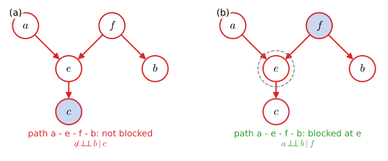
trails; \(f\) blocks it too). Redraws Bishop and Bishop (2024), Figure 11.21. Download: PDF · SVGp. 344 Parameters drawn as floating nodes (such as \(\lambda\)) behave like observed nodes, but since they have no parents every path through them is tail-to-tail and blocked: they play no role in d-separation. I.i.d. data. In Figure 11.12 the only path from \(\hat t\) to any \(t_n\) is \(\hat t\leftarrow\bw\to t_n\), tail-to-tail at \(\bw\); conditioning on \(\bw\) blocks it:
\[ \hat t\indep t_n\given\bw. \tag{11.36} \]So once the posterior over \(\bw\) (or an approximation such as \(\bw_{\mathrm{MAP}}\)) is computed, the training data can be discarded (Filling the gap 11.5). Without conditioning on \(\bw\) the path is open: the training targets are informative about \(\hat t\), which is the whole point of learning.
11.2.4 Naive Bayes
See also the companion course, Filling the gap 8.7 and naive Bayes with discrete features in Filling the gap 4.4; in this course, generative classifiers in Section 5.3.
pp. 344–346 The naive Bayes model splits the input into \(L\) parts \(\bx=(\bx^{(1)},\dots,\bx^{(L)})\) and assumes them independent given the class:
\[ p(\bx\given\Cc_k)=\prod_{l=1}^{L}p(\bx^{(l)}\given\Cc_k), \tag{11.37} \]the graph \(\Cc_k\to\bx^{(l)}\) for each \(l\) (Figure 11.22). Paths between parts are tail-to-tail at the class, blocked when the class is observed and open otherwise: the marginal \(p(\bx)\) does not factorise in general. Classification uses
\[ p(\Cc_k\given\bx)=\frac{p(\bx\given\Cc_k)p(\Cc_k)}{p(\bx)}, \tag{11.38} \] \[ p(\bx)=\sum_{k=1}^{K}p(\bx\given\Cc_k)p(\Cc_k). \tag{11.39} \]Result 11.11 (maximum likelihood for naive Bayes) p. 345; Exercise 11.15
Let \(p(\bx^{(l)}\given\Cc_k)\) have its own parameters \(\bw_k^{(l)}\) for each class \(k\) and part \(l\), and class priors \(\pi_k=p(\Cc_k)\). Given labelled data \(\{(\bx_n,\bt_n)\}\) (1-of-\(K\) labels \(t_{nk}\)), the maximum likelihood solution is
- \(\pi_k=N_k/N\), the fraction of points in class \(k\);
- \(\bw_k^{(l)}\) maximises \(\sum_{n:\,t_{nk}=1}\ln p(\bx_n^{(l)}\given\bw_k^{(l)})\): each part of each class is fitted on its own, to the \(l\)th part of that class's data only.
If the parameters \(\bw^{(l)}\) are shared across classes (as the book's wording allows), the second step becomes one fit of \(\bw^{(l)}\) to \(\sum_n\sum_kt_{nk}\ln p(\bx_n^{(l)}\given\Cc_k,\bw^{(l)})\), still separate for each part.
Proof (Exercise 11.15)
For i.i.d. data the log likelihood is \[\ln L=\sum_{n=1}^{N}\sum_{k=1}^{K}t_{nk}\Big[\ln\pi_k+\sum_{l=1}^{L}\ln p(\bx_n^{(l)}\given\bw_k^{(l)})\Big]=\sum_kN_k\ln\pi_k+\sum_k\sum_l\Big[\sum_{n:\,t_{nk}=1}\ln p(\bx_n^{(l)}\given\bw_k^{(l)})\Big].\] It is a sum of separate terms: one in \(\bpi\) only, and one for each pair \((k,l)\) in \(\bw_k^{(l)}\) only. Maximising a sum of functions of disjoint parameter blocks means maximising each term. For \(\bpi\) under \(\sum_k\pi_k=1\), the Lagrangian \(\sum_kN_k\ln\pi_k+\nu(\sum_k\pi_k-1)\) gives \(N_k/\pi_k=-\nu\), so \(\pi_k\propto N_k\) and \(\pi_k=N_k/N\) (Result 3.3). A numerical experiment maximises the likelihood of a two-class Gaussian naive Bayes model numerically and recover the class fraction and the per-class, per-feature means and variances. ∎
pp. 345–346 With two axis-aligned Gaussian classes in two dimensions,
\[ p(\bx\given\Cc_k)=p(x_1\given\Cc_k)p(x_2\given\Cc_k), \tag{11.40} \] \[ p(\bx)=\sum_{k=1}^{K}p(\bx\given\Cc_k)p(\Cc_k), \tag{11.41} \]a mixture of two Gaussians that does not factorise (Figure 11.23).
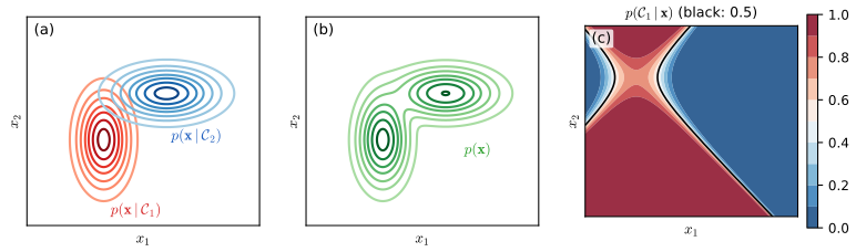
Filling the gap 11.7: why the mixture is dependent, and what naive Bayes boundaries look like pp. 345–346, Figure 11.23
Derivation
Dependence of the mixture. Within a class \(x_1\) and \(x_2\) are independent, so their covariance in the mixture comes only from the class means (law of total covariance): \[\cov[x_1,x_2]=\E_k\big[\cov[x_1,x_2\given\Cc_k]\big]+\cov_k\big[\E[x_1\given\Cc_k],\E[x_2\given\Cc_k]\big]=0+\sum_k\pi_k(\mu_{k1}-\bar\mu_1)(\mu_{k2}-\bar\mu_2).\] In Figure 11.23, \(\bar\bmu=(0.465,0.52)\) and the covariance is \[0.5(-0.135)(-0.1)+0.5(0.135)(0.1)=0.0135>0:\] nonzero covariance implies dependence. (The mixture would factorise only in degenerate cases, e.g. when the class conditionals of one coordinate coincide.)
Additive log-odds. By (11.37), the log posterior odds are a sum over parts: \[\ln\frac{p(\Cc_1\given\bx)}{p(\Cc_2\given\bx)}=\ln\frac{\pi_1}{\pi_2}+\sum_{l=1}^{L}\ln\frac{p(\bx^{(l)}\given\Cc_1)}{p(\bx^{(l)}\given\Cc_2)}.\] Each part contributes evidence separately, which is why naive Bayes fuses heterogeneous sources so easily (the blood test and skin image of Section 5.2.4). For Gaussian parts each term is a quadratic in its own \(x_l\) with no cross terms, \(a_lx_l^2+b_lx_l+c_l\) with \(a_l=\frac{1}{2\sigma_{2l}^2}-\frac{1}{2\sigma_{1l}^2}\), so the boundary is a conic with axes parallel to the coordinate axes. In Figure 11.23 class 1 is narrower in \(x_1\) and wider in \(x_2\), so \(a_1<0<a_2\) and the conic is a hyperbola, as panel (c) shows. With equal variances across classes the quadratic terms cancel and the boundary is linear (Section 5.3.1). ∎
p. 346 Naive Bayes helps when \(D\) is large (one-dimensional densities are much easier to estimate than a \(D\)-dimensional one) and when the input mixes discrete and continuous parts. Its assumption is strong and usually false, but classification can still be good because the decision depends on the class-conditional densities only through the boundary (Figure 5.8).
11.2.5 Generative models
See also the companion course, Section 8.1.2 and Result 8.3.
pp. 346–347 Many learning problems are inverse problems: a physical process turns causes (an object's class, position and scale) into data (an image), and we want to go back. A discriminative model, such as a convolutional network trained on labelled images, learns the inverse map directly and cannot use unlabelled images. A generative model describes the forward process (Figure 11.24: class, position and scale, independent a priori, each with an arrow into the image) and inverts it by inference. Once trained, it can also generate: draw the causes from their priors and then an image given them. That is ancestral sampling.
Algorithm 11.2 (ancestral sampling) p. 347
Number the nodes topologically. For \(k=1,\dots,K\): draw \(\hat x_k\sim p(x_k\given\pa_k=\hat\pa_k)\), using the values already drawn for the parents. Return \((\hat x_1,\dots,\hat x_K)\).
Result 11.12 (ancestral sampling is exact)
The returned vector has distribution (11.6), and any sub-vector is a draw from the corresponding marginal.
Proof
By induction on \(k\): if \((\hat x_1,\dots,\hat x_{k-1})\) has distribution \(\prod_{j<k}p(x_j\given\pa_j)\), which by Result 11.1(2) is the marginal of the first \(k-1\) variables, then drawing \(\hat x_k\) from \(p(x_k\given\pa_k)\) multiplies by the next factor. Marginals come for free by ignoring coordinates. A numerical experiment samples \(2\times10^5\) draws from the network of Figure 11.2 (largest frequency error 0.0013) and the linear-Gaussian chain of Figure 11.S3. ∎
p. 347 In Figure 11.24 every path between class, position and scale is head-to-head at the unobserved image, so they are independent a priori. Observing an image unblocks the paths: told the object's class, our belief about its position changes. Latent variables need not have a physical meaning: normalising flows, variational autoencoders and diffusion models (Chapters 18 to 20 of the book) push a simple Gaussian latent through a deep network to make a complex distribution, and ancestral sampling is how they generate.
11.2.6 Markov blanket
See also the companion course, Result 8.10.
pp. 347–348 The conditional of one node given all the others is
\[ p(x_i\given\bx_{\{j\ne i\}})=\frac{p(x_1,\dots,x_D)}{\int p(x_1,\dots,x_D)\,\d x_i}=\frac{\prod_kp(x_k\given\pa_k)}{\int\prod_kp(x_k\given\pa_k)\,\d x_i}. \]Result 11.13 (the Markov blanket) p. 348, Figure 11.25; Exercise 11.12
Let \(\MB(x_i)\) be the parents, the children and the co-parents (the other parents of the children) of \(x_i\). Then \[p(x_i\given\bx_{\{j\ne i\}})=p(x_i\given\MB(x_i))\propto p(x_i\given\pa_i)\prod_{k:\,i\in\pa_k}p(x_k\given\pa_k),\] i.e. \(x_i\indep(\text{all other nodes})\given\MB(x_i)\). No member can be dropped in general: for each \(y\in\MB(x_i)\) some distribution in \(\DF\) has \(x_i\nindep y\given\MB(x_i)\setminus\{y\}\).
Proof
By factorisation. Factors without \(x_i\) do not depend on the integration variable, come out of the integral and cancel. The factors with \(x_i\) are its own, a function of \(x_i\) and \(\pa_i\), and those of its children, functions of the child, \(x_i\) and the co-parents. So the ratio depends only on \(x_i\) and \(\MB(x_i)\).
By d-separation (Exercise 11.12). Take any path from \(x_i\) to a node \(y\notin\MB(x_i)\cup\{x_i\}\). If its first step goes to a parent \(p\), the path leaves \(p\) by its tail (\(p\to x_i\)), so \(p\) is head-to-tail or tail-to-tail on it and observed: blocked. If the first step goes to a child \(c\), the next node is either a child of \(c\) (then \(c\) is head-to-tail and observed: blocked) or another parent \(q\) of \(c\) (then \(c\) is an observed collider and lets the path through; but the path meets the co-parent \(q\) at the tail of the arrow \(q\to c\), so \(q\) is a non-collider on the path, and it is observed: blocked). \(y\) itself cannot be the second node, since all nodes at distance one or two of this kind are in the blanket.
Minimality. A parent or child is joined to \(x_i\) by a link, a path that nothing can block. For a co-parent \(q\) of child \(c\), the path \(x_i\to c\leftarrow q\) with \(c\) observed is open. By the completeness half of Result 11.10, some distribution in \(\DF\) shows the dependence. This is the book's remark that observing only parents and children is not enough because of explaining away. A direct computation verifies the blanket by enumeration on 15 random seven-node networks, and that dropping a co-parent in Figure 11.25 leaves \(I>0\). ∎
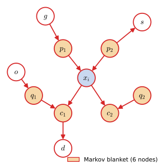
markov_blanket: parents \(p_1,p_2\), children \(c_1,c_2\) and co-parents \(q_1,q_2\) (orange). The grandparent \(g\), the grandchild \(d\), the parent's other child \(s\) and the co-parent's parent \(o\) are outside it. Redraws Bishop and Bishop (2024), Figure 11.25, on a concrete graph. Download: PDF · SVG11.2.7 Graphs as filters
See also the companion course, Result 8.9(b).
pp. 348–349 A graph acts as two filters on the set of all distributions over its variables: one passes the distributions that factorise as (11.6), the set \(\DF\); the other passes those that satisfy every conditional independence that d-separation reads off the graph, call it \(\DI\). The book states that the two sets coincide (Figure 11.26). Half of this is Result 11.10(1); the other half has a short proof that uses only the tools above.
Result 11.14 (the two filters pass the same distributions: \(\DF=\DI\)) pp. 348–349, Figure 11.26
Lemma. In a topological numbering, \(\pa_k\) d-separates \(x_k\) from every earlier node that is not a parent.
Theorem. \(\DF=\DI\). In particular a fully connected graph passes every distribution, and a fully factorised distribution passes every graph.
Proof
Lemma. Let \(u<k\), \(u\notin\pa_k\), and take a path from \(x_k\) to \(u\). If it starts at a parent \(p\) of \(x_k\), it leaves \(p\) by a tail, so \(p\) is a non-collider in \(C=\pa_k\): blocked. Otherwise it starts \(x_k\to c_1\). Follow it while it keeps going along arrows: \(x_k\to c_1\to c_2\to\cdots\), all descendants of \(x_k\), hence numbered above \(k\). Since it ends at \(u<k\), it must at some point go against an arrow; the first time it does, at node \(c_m\), the path meets \(c_m\) head-to-head. \(c_m\) and all its descendants are descendants of \(x_k\), numbered above \(k\), while every node of \(C=\pa_k\) is numbered below \(k\). So no descendant of the collider is observed: blocked.
\(\DI\subseteq\DF\). If \(p\) satisfies all d-separation statements, the Lemma gives \(x_k\indep\{x_1,\dots,x_{k-1}\}\setminus\pa_k\given\pa_k\) for every \(k\), which is the ordered Markov property, equivalent to factorisation by Filling the gap 11.1.
\(\DF\subseteq\DI\) is soundness, Result 11.10(1).
The fully connected graph has no d-separation statements at all, so \(\DI\) is everything. A fully factorised distribution satisfies every independence statement, so it is in \(\DI\) for every graph, hence in \(\DF\). ∎
The theorem is about families: a particular distribution in \(\DF\) may have extra independences (for special values of its tables) that the graph does not show, as the measure-zero exceptions of Result 11.8 illustrate. The statements also hold whether the variables are discrete, continuous or mixed.
11.3 Sequence Models
See also the companion course, Section 13.1 (Markov models), Results 13.1–13.3, and autoregressive models.
pp. 349–350 Text, proteins, audio and rainfall records are sequences \(\bx_1,\dots,\bx_N\); "time", "past" and "future" refer to positions in the sequence. Several independent sequences have a joint distribution that is a product over sequences, so it suffices to model one. Ordering the chain rule (11.4) along the sequence gives the autoregressive factorisation
\[ p(\bx_1,\dots,\bx_N)=\prod_{n=1}^{N}p(\bx_n\given\bx_1,\dots,\bx_{n-1}), \tag{11.42} \]the fully connected graph of Figure 11.27. It holds for every distribution, so it assumes nothing; assumptions enter by deleting links. Deleting all of them treats the elements as independent,
\[ p(\bx_1,\dots,\bx_N)=\prod_{n=1}^{N}p(\bx_n), \tag{11.43} \]which ignores the order altogether (Figure 11.28). Keeping only the link from the previous element gives a (first-order) Markov chain,
\[ p(\bx_1,\dots,\bx_N)=p(\bx_1)\prod_{n=2}^{N}p(\bx_n\given\bx_{n-1}), \tag{11.44} \](Figure 11.29), for which
\[ p(\bx_n\given\bx_1,\dots,\bx_{n-1})=p(\bx_n\given\bx_{n-1}). \tag{11.45} \]Keeping two gives the second-order chain (Figure 11.30)
\[ p(\bx_1,\dots,\bx_N)=p(\bx_1)p(\bx_2\given\bx_1)\prod_{n=3}^{N}p(\bx_n\given\bx_{n-1},\bx_{n-2}), \tag{11.46} \]with
\[ p(\bx_n\given\bx_1,\dots,\bx_{n-1})=p(\bx_n\given\bx_{n-1},\bx_{n-2}), \tag{11.52} \]and in general an \(M\)th-order chain conditions on the previous \(M\) elements.
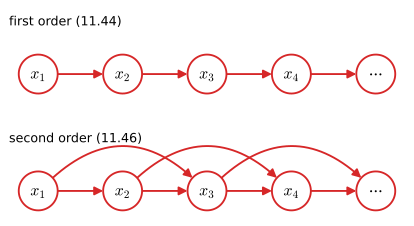
Result 11.15 (the Markov properties (11.45) and (11.52)) p. 351; Exercises 11.16, 11.17
The chain (11.44) satisfies (11.45) for \(n=2,\dots,N\); the chain (11.46) satisfies (11.52) for \(n=3,\dots,N\); an \(M\)th-order chain satisfies \(p(\bx_n\given\bx_{1:n-1})=p(\bx_n\given\bx_{n-M:n-1})\). In words, the future is independent of the distant past given the last \(M\) values.
Proof (Exercises 11.16 and 11.17)
By the sum and product rules. Summing (11.44) over \(\bx_N\), then \(\bx_{N-1}\), ..., \(\bx_{n+1}\) (each sum removes one factor that sums to one, the last remaining factor being the only one containing the summed variable) gives \(p(\bx_1,\dots,\bx_n)=p(\bx_1)\prod_{m=2}^{n}p(\bx_m\given\bx_{m-1})\). Dividing by the same expression with \(n-1\) gives \(p(\bx_n\given\bx_1,\dots,\bx_{n-1})=p(\bx_n\given\bx_{n-1})\), which is (11.45). The same steps on (11.46) leave \(p(\bx_n\given\bx_{n-1},\bx_{n-2})\), which is (11.52). This is Result 11.1(3) for these graphs.
By d-separation. In an \(M\)th-order chain \(\pa(\bx_n)=\{\bx_{n-M},\dots,\bx_{n-1}\}\) and the numbering is topological, so the Lemma of Result 11.14 says the parents d-separate \(\bx_n\) from \(\bx_1,\dots,\bx_{n-M-1}\). For the first-order chain this is visible directly: the only path from \(\bx_m\) (\(m<n-1\)) to \(\bx_n\) runs along the chain and passes \(\bx_{n-1}\) head-to-tail; the second-order chain has more paths, including ones that go beyond \(n\) and come back through a collider, which is why the general Lemma is the clean argument. A direct computation confirms both properties by conditional mutual information on random three-state chains of length 6, and that a second-order chain is not first-order. ∎
pp. 351–352 The price of a longer memory is the number of parameters.
Result 11.16 (parameters of an \(M\)th-order chain) p. 352
For \(K\)-state variables and a general conditional probability table shared over \(n\) (a homogeneous chain), the table \(p(\bx_n\given\bx_{n-M},\dots,\bx_{n-1})\) has \(K^M(K-1)\) free parameters, plus \(K^M-1\) for the distribution of the first \(M\) values. The count grows exponentially in \(M\).
Erratum (p. 352): the book gives \(K^{M-1}(K-1)\). For \(M=1\) that is \(K-1\), contradicting the \(K(K-1)\) stated for the first-order chain in the sentence before. (The same slip appears in Bishop (2006), p. 609; see the companion course's Result 13.3.)
Proof
The conditioning tuple has \(K^M\) configurations, each needing a distribution over \(K\) values, \(K-1\) free numbers: \(K^M(K-1)\). The first \(M\) values have a general joint table, \(K^M-1\) (equivalently, the book's \(p(\bx_1)p(\bx_2\given\bx_1)\cdots\), which has \((K-1)(1+K+\dots+K^{M-1})\) \(=K^M-1\)). Counting table entries directly for \(M=1,\dots,4\) agrees. ∎
How are these tables fitted, and how large should \(M\) be? The book does not say. On real data the answers are instructive, and they are the subject of the third demo.
Result 11.17 (maximum likelihood for a Markov chain is counting)
Let \(n(s,x)\) be the number of times symbol \(x\) follows the context \(s\) (the previous \(M\) symbols) in the training sequence, and \(n(s)=\sum_xn(s,x)\). The maximum likelihood transition table is \[\hat p(x\given s)=\frac{n(s,x)}{n(s)}\quad(n(s)>0),\] and with a symmetric Dirichlet prior of parameter \(\alpha\) on each row, the posterior mean is the additively smoothed estimate \[\tilde p(x\given s)=\frac{n(s,x)+\alpha}{n(s)+K\alpha}.\]
Proof
Conditioned on the first \(M\) symbols, the log likelihood of the training sequence under a homogeneous order-\(M\) chain is \[\sum_{n}\ln p(x_n\given s_n)=\sum_s\sum_xn(s,x)\ln\theta_{x\given s}:\] a separate categorical log likelihood for each context. Each is maximised under \(\sum_x\theta_{x\given s}=1\) by the normalised counts (Lagrange multiplier, as in Result 3.3). With a Dirichlet\((\alpha,\dots,\alpha)\) prior the posterior of row \(s\) is Dirichlet\((n(s,x)+\alpha)\), whose mean is \(\tilde p\) (companion course Section 2.2.1). A direct computation confirms that 200 random feasible perturbations of the counted row for the context "the" all lower the likelihood. ∎
Filling the gap 11.8: what the exponential parameter count does on real text p. 352
The book's remark that large \(M\) is "impractical" can be made quantitative. The text of Lewis Carroll's Alice's Adventures in Wonderland, reduced to \(K=28\) symbols (space, full stop, a to z), has 122,778 training characters and 13,640 held-out ones. Fit an order-\(k\) chain by smoothed counts and measure the held-out cross-entropy \(-\frac1n\sum_i\log_2\tilde p(x_i\given s_i)\) in bits per character.
Derivation and numbers
What the cross-entropy measures. For a stationary source, the average of \(-\log_2\tilde p(x_i\given s_i)\) over held-out text estimates \(H(p_{\text{data}})+\KL(p_{\text{data}}\,\|\,\tilde p)\) per symbol (Section 2.5.5), so it is minimised by the true conditional and penalises a model for every bit of misplaced probability. The uniform model scores \(\log_228=4.81\) bits; letter frequencies alone (\(k=0\)) 4.12 bits.
Two errors pull in opposite directions. Small \(k\) is biased: it cannot represent dependences longer than \(k\). Large \(k\) has \(28^k\cdot27\) parameters but at most 122,778 training positions, so most contexts are never or rarely seen: at \(k=4\) the text visits 10,657 of the \(614{,}656\) possible contexts, at \(k=10\) 92,349 of \(3\times10^{14}\). An unseen context gets a uniform row (with smoothing) or no row at all (maximum likelihood), and a seen context with one occurrence gets a row that is mostly smoothing. The training cross-entropy keeps falling with \(k\) (0.46 bits at \(k=10\), \(\alpha=0.01\): the model memorises), while the held-out one has a minimum:
| order \(k\) | 0 | 1 | 2 | 3 | 4 | 5 | 6 | 8 | 10 |
|---|---|---|---|---|---|---|---|---|---|
| \(\alpha=1\) | 4.12 | 3.25 | 2.58 | 2.38 | 2.64 | 3.06 | 3.47 | 4.10 | 4.46 |
| \(\alpha=0.1\) | 4.12 | 3.25 | 2.53 | 2.13 | 2.16 | 2.44 | 2.82 | 3.58 | 4.13 |
| \(\alpha=0.1\), back off | 4.12 | 3.25 | 2.53 | 2.12 | 2.12 | 2.23 | 2.36 | 2.58 | 2.67 |
(held-out bits per character; bold: the best order in each row). "Back off" gives an unseen context the row of its longest suffix that was seen. That is parameter tying in the sense of Section 11.1.3, and the model remains an order-\(k\) chain with normalised conditionals; it removes most of the damage from large \(k\) but still has its optimum at \(k=4\) (2.117 bits). With \(\alpha=0\) any held-out symbol that never followed its context in training has probability zero and the held-out cross-entropy is infinite, for every \(k\ge1\).
Samples (110 characters after the prompt "alice was beginning to get very tired ", seed 3, back off):
k = 0:  o g phh ai  ohrtdnbnisi tdureo eo  htlnrkj eiseghirtnenogwtonur  iteicgiiep unor e nrlyywktusdmuel miat s et n
k = 1:  s l the ff asertararere t. the ir ansheree inond outhengayothro ans. gang. curou iderivowhowiketef se t t it s
k = 2:  teldeen do and the shin this sain aming on her known hemayings a much ing thoust i sompty ust roqueen ter it s
k = 3:  the she flaminuted the as wher he and to large king. in. you wonder neveral whit joings.blowledgehog grave tal
k = 5:  off the end of the pleaded. what a great had somebody seemed to alice in bringing down. would not answered the
k = 10: of being such a noise inside no one could possibly reach it. she could not even get her head made her so savag
(\(\alpha=0.01\) for \(k\le3\), 0.001 for \(k=5\), 0 for \(k=10\)). The order-10 sample is copied from the book: plausible locally, it is memorisation, and the same model assigns zero probability to held-out text. Shannon (1948) made the same experiment by hand with letter tables of English. Every number here is recomputed by the Python code and reproduced by the demo. ∎
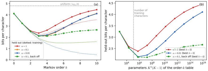
Exercise 11.18 (below) shows that higher order is not a different kind of model: grouping \(M\) consecutive values into one variable turns an \(M\)th-order chain into a first-order one on \(K^M\) states, which again shows the exponential cost.
11.3.1 Hidden variables
See also the companion course, Result 13.4, Section 13.2 (hidden Markov models) and Section 13.3 (linear dynamical systems), with the HMM demo and the Kalman filter demo.
pp. 352–353 To model long-range dependence with few parameters, attach to each observation \(\bx_n\) a latent variable \(\bz_n\) and let the latent variables form the Markov chain: the state-space model of Figure 11.31. It has
\[ \bz_{n+1}\indep\bz_{n-1}\given\bz_n, \tag{11.47} \] \[ p(\bx_1,\dots,\bx_N,\bz_1,\dots,\bz_N)=p(\bz_1)\Big[\prod_{n=2}^{N}p(\bz_n\given\bz_{n-1})\Big]\prod_{n=1}^{N}p(\bx_n\given\bz_n). \tag{11.48} \]With discrete \(\bz_n\) it is a hidden Markov model (Elliott, Aggoun and Moore, 1995); with linear-Gaussian conditionals for both \(\bz\) and \(\bx\) it is a linear dynamical system, whose exact inference algorithm is the Kalman filter (Zarchan and Musoff, 2005; the book calls the model itself a Kalman filter). Replacing the emission tables or linear maps \(p(\bx_n\given\bz_n)\) by deep networks makes either much more flexible.
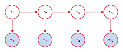
Result 11.18 (latent chains: Markov states, non-Markov observations) pp. 352–353, (11.47); Exercise 11.19
- The latent chain satisfies (11.47) and, marginally, is the Markov chain \(p(\bz_1)\prod_np(\bz_n\given\bz_{n-1})\).
- The observations satisfy no conditional independence of the form \(\bx_{n+1}\indep\bx_{n-k}\given\bx_{n-k+1},\dots,\bx_n\) for any \(k\): they are not Markov of any finite order. For generic parameters the dependence is real, and it decays with \(k\).
Proof (Exercise 11.19)
(1) Summing (11.48) over all \(\bx_n\) removes every emission factor (each sums to 1), leaving the Markov chain (11.44) for \(\bz\); (11.47) is then Result 11.15. By d-separation: every path from \(\bz_{n+1}\) to \(\bz_{n-1}\) passes \(\bz_n\), as a head-to-tail node along the chain (paths through an \(\bx\) node are impossible, since each \(\bx_m\) has a single neighbour), so observing \(\bz_n\) blocks it.
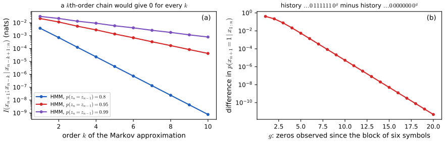
(2) Consider the path \[\bx_{n-k}\leftarrow\bz_{n-k}\to\bz_{n-k+1}\to\cdots\to\bz_{n+1}\to\bx_{n+1}.\] Its interior nodes are latent: \(\bz_{n-k}\) is tail-to-tail and the others head-to-tail, none observed, so with \(C=\{\bx_{n-k+1},\dots,\bx_n\}\) the path is open (observed \(\bx\)'s are not on it). So the independence is not implied, and by completeness (Result 11.10) it fails for some, indeed generic, parameters. Numerically, for a two-state HMM with \(p(\bz_n=\bz_{n-1})=0.95\) and emissions that are right with probability 0.8, \(I(x_{n+1};x_{n-k}\given x_{n-k+1:n})\) is 0.021, 0.011, 0.0054, 0.0013 and 0.00017 nats for \(k=1,2,3,5,8\), each extra symbol of context removing about half of what is left (Figure 11.S5). The book's sentence "our predictions for \(\bx_{n+1}\) depend on all previous observations" is exactly this. ∎
The state-space model has a finite set of parameters (initial, transition and emission distributions), yet its predictions use the whole past. How is that computed, and what does it have to do with the neural sequence models of the later chapters? The book stops here; the connection is worth making.
Filling the gap 11.9: the predictive distribution is a recurrent network, and the step to neural sequence models p. 353
Derivation
The filtering recursion. For an HMM with transition matrix \(A_{jk}=p(z_n=k\given z_{n-1}=j)\) and emissions \(e_k(x)=p(x\given z=k)\), define the normalised forward vector \(\hat\alpha_n(k)=p(z_n=k\given x_1,\dots,x_n)\). By the product and sum rules and (11.48), \[\hat\alpha_n(k)=\frac{e_k(x_n)\sum_j\hat\alpha_{n-1}(j)A_{jk}}{\sum_{k'}e_{k'}(x_n)\sum_j\hat\alpha_{n-1}(j)A_{jk'}},\qquad p(x_{n+1}\given x_1,\dots,x_n)=\sum_k\Big(\sum_j\hat\alpha_n(j)A_{jk}\Big)e_k(x_{n+1}).\] The first step uses \(x_n\indep x_{1:n-1}\given z_n\) and \(z_n\indep x_{1:n-1}\given z_{n-1}\), both d-separation statements of Figure 11.31. A direct computation confirms that this recursion gives exactly the ratio \(p(x_{1:n+1})/p(x_{1:n})\) computed by summing over all latent paths.
Reading it as a network. The whole past is summarised by a fixed-size state \(\hat\alpha_n\in\R^K\), updated by a fixed function of the previous state and the new input, \(\hat\alpha_n=f(\hat\alpha_{n-1},x_n)\), and read out to give the next-symbol distribution. That is exactly the structure of a recurrent neural network, with a hand-specified, normalised, linear-then-multiplicative update instead of a learned one. Because the state is a probability vector updated by a contraction (each step mixes through \(A\)), old inputs are forgotten geometrically, which is the decay seen in Figure 11.S5.
Neural autoregressive models. A modern language model goes back to (11.42) itself, \[p(x_n\given x_1,\dots,x_{n-1})=\mathrm{softmax}\big(f_\theta(x_1,\dots,x_{n-1})\big),\] with one network \(f_\theta\) shared across positions. It makes no Markov assumption (any context length) and has no latent state to infer, yet its parameter count does not grow with the context, unlike the \(K^M(K-1)\) of a table. Parameter sharing across positions, the device of Figure 11.5, is what makes it feasible; a recurrent network compresses the past into a learned state, a transformer (Chapter 12 of the book) attends to all of it. Sampling is ancestral sampling along the sequence. ∎
Corrections to the book
The first printing of Chapter 11 has these slips (there is no solutions manual for this chapter to compare with). Each is confirmed numerically where a number is involved.
- p. 352, parameter count of an \(M\)th-order Markov chain. Printed \(K^{M-1}(K-1)\); correct \(K^M(K-1)\). At \(M=1\) the printed formula gives \(K-1\), contradicting the \(K(K-1)\) of the sentence before (Result 11.16).
- p. 333, (11.13). The covariance recursion holds only when \(x_i\) is not a descendant of \(x_j\) (e.g. \(i\le j\) in a topological numbering); read for all \(i,j\) it gives \(\cov[x_2,x_1]=0\) for \(x_1\to x_2\), instead of \(w_{21}v_1\) (Result 11.5).
- p. 334 and Figures 11.10, 11.11. The binary classifier "contains the noise variance \(\sigma^2\)": a Bernoulli likelihood has no noise variance; \(\sigma^2\) and the phrase "linear regression model" on p. 335 are carried over from the regression version of the example.
- p. 354, Exercise 11.5. "The parameters \(\mu_i\) represent the probabilities \(p(x_i=1)\)": in the noisy-OR (11.49), \(\mu_i\) is the probability that cause \(i\) on its own switches \(y\) on (with \(\mu_0=0\), \(\mu_i=p(y=1\given x_i=1,\ x_{j\ne i}=0)\)); \(p(x_i=1)\) is the separate prior parameter of the parents in Figure 11.6.
- p. 353, terminology. A linear dynamical system is "also known as a Kalman filter": the Kalman filter is the exact inference (filtering) algorithm for that model, not the model.
- Typographical: p. 346 "learn now to invert this process" (how), "proving the labels" (providing); p. 350 "a specific of ordering" (a specific ordering).
Exercises
All 19 exercises of Chapter 11 (Bishop and Bishop, 2024, pp. 353–356), restated in my own words, with complete solutions (hidden). Stars give the book's difficulty. The official solutions manual does not cover this chapter; every numerical answer was confirmed by direct computation.
Exercise 11.1 (★). Show, by summing out the variables one at a time, that the directed factorisation (11.6) is normalised whenever each conditional is.
Solution
Number the nodes topologically. \(x_K\) has no children, so it appears only in \(p(x_K\given\pa_K)\), and \(\sum_{x_K}p(x_K\given\pa_K)=1\) for every value of \(\pa_K\). What is left is the factorisation of the graph with node \(K\) deleted, which is again a DAG with a childless last node. After \(K\) steps the total is 1. Full details, including that the factors are the conditionals of the joint: Result 11.1.
Exercise 11.2 (★). Show that if the nodes can be numbered so that no link goes to a lower-numbered node, the graph has no directed cycles.
Solution
Numbers strictly increase along every directed path, so no path returns to its start. The converse (every DAG has such a numbering) is also true: Result 11.2.
Exercise 11.3 (★★). For the joint distribution of three binary variables in Table 11.1 (\(p(a,b,c)\) for \((a,b,c)=000,\dots,111\): 0.192, 0.144, 0.048, 0.216, 0.192, 0.064, 0.048, 0.096), show that \(p(a,b)\ne p(a)p(b)\) but \(p(a,b\given c)=p(a\given c)p(b\given c)\) for \(c=0\) and \(c=1\).
Solution
Marginals. \[p(a=0)=0.192+0.144+0.048+0.216=0.6,\qquad p(b=0)=0.192+0.144+0.192+0.064=0.592,\] and \(p(a=0,b=0)=0.192+0.144=0.336\), while \(p(a=0)p(b=0)=0.3552\ne0.336\). So \(a\) and \(b\) are dependent.
Given \(c=0\) (\(p(c=0)=0.48\)): the table of \(p(a,b\given c=0)\) for \((a,b)=00,01,10,11\) is \(0.4,0.1,0.4,0.1\); \(p(a=0\given c=0)=0.5\), \(p(b=0\given c=0)=0.8\), and \(0.5\times0.8=0.4\), \(0.5\times0.2=0.1\), and the same for \(a=1\). Independent.
Given \(c=1\) (\(p(c=1)=0.52\)): \[p(a,b\given c=1)=\frac{(0.144,\,0.216,\,0.064,\,0.096)}{0.52}\] for \((a,b)=00,01,10,11\), with \(p(a=0\given c=1)=0.36/0.52=9/13\) and \(p(b=0\given c=1)=0.208/0.52=0.4\). Check: \[\tfrac{9}{13}\cdot0.4=\tfrac{0.144}{0.52},\quad \tfrac{9}{13}\cdot0.6=\tfrac{0.216}{0.52},\quad \tfrac{4}{13}\cdot0.4=\tfrac{0.064}{0.52},\quad \tfrac{4}{13}\cdot0.6=\tfrac{0.096}{0.52}.\] Independent. (Checked numerically.)
Exercise 11.4 (★★). For Table 11.1, compute \(p(a)\), \(p(b\given c)\) and \(p(c\given a)\), verify \(p(a,b,c)=p(a)p(c\given a)p(b\given c)\) and draw the graph.
Solution
\(p(a=1)=0.4\). From the table, \(p(a,c)\) for \((a,c)=00,01,10,11\) is \(0.24,0.36,0.24,0.16\), so \(p(c=1\given a=0)=0.6\) and \(p(c=1\given a=1)=0.4\). Also \(p(b=1,c=0)=0.048+0.048=0.096\) and \(p(c=0)=0.48\), so \(p(b=1\given c=0)=0.2\); \(p(b=1,c=1)=0.216+0.096=0.312\) and \(p(c=1)=0.52\), so \(p(b=1\given c=1)=0.6\).
Product, e.g. \((a,b,c)=(0,0,0)\): \(0.6\times0.4\times0.8=0.192\); \((0,1,1)\): \(0.6\times0.6\times0.6=0.216\); \((1,0,1)\): \(0.4\times0.4\times0.4=0.064\); \((1,1,1)\): \(0.4\times0.4\times0.6=0.096\); the other four agree likewise (all eight are checked). The graph is the head-to-tail chain \(a\to c\to b\), consistent with Exercise 11.3 and Result 11.8(2). (The tail-to-tail graph \(a\leftarrow c\to b\) describes the same independences, and by reversing the arrow \(a\to c\) with Bayes' theorem it fits the same table.) The demo has this table as a network.
Exercise 11.5 (★). The noisy-OR \[p(y=1\given x_1,\dots,x_M)=1-(1-\mu_0)\prod_{i=1}^{M}(1-\mu_i)^{x_i},\tag{11.49}\] with \(0\le\mu_0\le1\), also uses \(M+1\) parameters. Interpret it as a soft logical OR and explain \(\mu_0\).
Solution
If all \(\mu_i=1\) and \(\mu_0=0\): any \(x_i=1\) makes the product 0, so \(p(y=1)=1\); with all \(x_i=0\), \(p(y=1)=0\). That is the OR. In general each active parent independently "fires" with probability \(\mu_i\), and \(y=1\) if anything fires (Filling the gap 11.2 derives (11.49) from this story). \(p(y=1\given\bx)\) never decreases when a parent is switched on. \(\mu_0\) is the leak: the probability that \(y=1\) when no parent is on, \(p(y=1\given\bx=\bzero)=\mu_0\), standing for causes not in the model. Erratum: the book calls \(\mu_i\) "the probabilities \(p(x_i=1)\)"; they are the probabilities that cause \(i\) alone switches \(y\) on (see Corrections). In the demo, seeing \(y=1\) raises \(p(x_2=1)\) from 0.2 to 0.43; learning \(x_1=1\) lowers it to 0.22.
Exercise 11.6 (★★). Derive the mean recursion (11.12) from (11.9).
Solution
(11.9) is \(x_i=\sum_{j\in\pa(i)}w_{ij}x_j+b_i+\sqrt{v_i}\epsilon_i\) with \(\epsilon_i\sim\N(0,1)\) independent of the parents. Taking expectations, \(\E[x_i]=\sum_jw_{ij}\E[x_j]+b_i\). In closed form, \(\bmu=(\bI-\bW)^{-1}\bb\) (Result 11.4, Result 11.5).
Exercise 11.7 (★★). Derive the covariance recursion (11.13).
Solution
\[\cov[x_i,x_j]=\sum_{k\in\pa(j)}w_{jk}\cov[x_i,x_k]+\sqrt{v_j}\cov[x_i,\epsilon_j],\] and \(\sqrt{v_j}\cov[x_i,\epsilon_j]=I_{ij}v_j\) provided \(x_i\) is not a descendant of \(x_j\). The proof and the counterexample for descendants are in Result 11.5; the recursion is applied to \(i\le j\) and completed by symmetry.
Exercise 11.8 (★★). Show that a fully connected linear-Gaussian graph over \(D\) variables has \(D(D+1)/2\) parameters in its covariance.
Solution
Node \(i\) has \(i-1\) weights: \(\sum_i(i-1)=D(D-1)/2\); plus \(D\) variances: \(D(D+1)/2\), the number of free entries of a symmetric matrix. Moreover the map from \((\bW,\bV)\) to \(\Sig\) is a bijection onto all positive definite matrices (Cholesky), so these are genuinely free: Result 11.6.
Exercise 11.9 (★★). Use the recursions to derive (11.14) and (11.15) for Figure 11.7.
Solution
Parents: \(\pa(1)=\emptyset\), \(\pa(2)=\{1\}\), \(\pa(3)=\{2\}\). Means: \(\mu_1=b_1\), \(\mu_2=w_{21}\mu_1+b_2\), and \(\mu_3=w_{32}\mu_2+b_3\), which is (11.14). Covariances, column by column with \(i\le j\): \[\begin{aligned}\Sigma_{11}&=v_1, & \Sigma_{12}&=w_{21}\Sigma_{11}=w_{21}v_1,\\ \Sigma_{22}&=w_{21}\Sigma_{21}+v_2=v_2+w_{21}^2v_1, & \Sigma_{13}&=w_{32}\Sigma_{12}=w_{32}w_{21}v_1,\\ \Sigma_{23}&=w_{32}\Sigma_{22}=w_{32}(v_2+w_{21}^2v_1), & \Sigma_{33}&=w_{32}\Sigma_{32}+v_3.\end{aligned}\] With \(\Sigma_{32}=\Sigma_{23}\) the last is \(v_3+w_{32}^2(v_2+w_{21}^2v_1)\), and symmetry gives (11.15). Checked against the closed form, and against 2000 ancestral samples in Figure 11.S3.
Exercise 11.10 (★). Verify that the vector-valued linear-Gaussian model (11.16) has a Gaussian joint distribution.
Solution
Stacking, \[\bx=(\bI-\bW)^{-1}(\bb+\bV^{1/2}\beps)\] with block lower triangular \(\bW\) and block diagonal \(\bV\): an affine image of a standard Gaussian, hence Gaussian. Equivalently \[\ln p(\bx)=-\frac12\sum_i\Big(\bx_i-\sum_j\bW_{ij}\bx_j-\bb_i\Big)^\T\Sig_i^{-1}\Big(\cdots\Big)+\const\] is a quadratic form in \(\bx\) with positive definite precision \((\bI-\bW)^\T\bV^{-1}(\bI-\bW)\). Block recursions: Filling the gap 11.4.
Exercise 11.11 (★). Show that \(a\indep b,c\given d\) implies \(a\indep b\given d\).
Solution
\(p(a,b,c\given d)=p(a\given d)p(b,c\given d)\); sum over \(c\): \(p(a,b\given d)=p(a\given d)p(b\given d)\). (Result 11.7(3); checked on a random table built to satisfy the premise.)
Exercise 11.12 (★). Using d-separation, show that a node is independent of all other nodes given its Markov blanket.
Solution
Every path from \(x_i\) to a node outside the blanket starts at a parent (an observed non-collider: blocked) or at a child \(c\); from \(c\) it continues either to a child of \(c\) (\(c\) is an observed head-to-tail node: blocked) or to a co-parent \(q\) (through the observed collider \(c\), but then \(q\) is an observed non-collider: blocked). Details in Result 11.13.
Exercise 11.13 (★). In the graph \(a\to c\leftarrow b\), \(c\to d\) (Figure 11.32), show that \(a\indep b\given\emptyset\), and that in general \(a\nindep b\given d\).
Solution
Summing \(p(a)p(b)p(c\given a,b)p(d\given c)\) over \(d\) and \(c\) gives \(p(a)p(b)\). Given \(d\), \(p(a,b\given d)\propto p(a)p(b)\tilde p(d\given a,b)\) with \(\tilde p(d\given a,b)=\sum_cp(d\given c)p(c\given a,b)\), which factorises in \((a,b)\) only for special tables. Concrete case: the fuel system with the driver's report \(D\) as \(d\): \(p(F=0\given D=0)=0.2125\) but \(p(F=0\given D=0,B=0)=0.1096\), so \(F\) and \(B\) are dependent given \(D\). See Result 11.9.
Exercise 11.14 (★★). In the fuel system, suppose we do not see the gauge but hear a driver \(D\) report it, with \(p(D=1\given G=1)=0.9\) (11.50) and \(p(D=0\given G=0)=0.9\) (11.51). Given \(D=0\), find the probability that the tank is empty; then given also \(B=0\). Explain why the second is lower and relate it to Figure 11.32.
Solution
Given \(D=0\). \[p(D=0)=0.9\,p(G=0)+0.1\,p(G=1)=0.9(0.315)+0.1(0.685)=0.352,\] \[p(D=0\given F=0)=0.9\,p(G=0\given F=0)+0.1\,p(G=1\given F=0)=0.9(0.81)+0.1(0.19)=0.748.\] Hence \[p(F=0\given D=0)=\frac{0.748\times0.1}{0.352}=0.2125.\]
Given also \(B=0\). \[p(D=0\given B=0,F=0)=0.9(0.9)+0.1(0.1)=0.82,\quad p(D=0\given B=0,F=1)=0.9(0.8)+0.1(0.2)=0.74,\] so \[p(F=0\given D=0,B=0)=\frac{0.82\times0.1}{0.82\times0.1+0.74\times0.9}=\frac{0.082}{0.748}=0.1096.\]
Why. Both are below the values for observing the gauge itself (0.257 and 0.111) because the driver adds noise: the likelihood ratios are pulled towards 1. The flat battery still explains away the empty report, because \(D\) is a descendant of the collider \(G\) in \(B\to G\leftarrow F\), \(G\to D\), exactly the graph of Figure 11.32 with \(a=B\), \(b=F\), \(c=G\), \(d=D\): observing \(D\) unblocks the path between \(B\) and \(F\) (Result 11.9). The value 0.1096 is still above the prior 0.1. Checked exactly; demo preset 3.
Exercise 11.15 (★★). Show that maximum likelihood for naive Bayes (11.37), with separate parameters for each part, fits each class-conditional density of each part to the corresponding data and sets the class priors to the class fractions.
Solution
The log likelihood splits into \(\sum_kN_k\ln\pi_k\) plus one term per (class, part) that depends only on that block's parameters; maximise each term separately, and \(\pi_k=N_k/N\) by a Lagrange multiplier. Full argument: Result 11.11 (numerically confirmed for a Gaussian naive Bayes model).
Exercise 11.16 (★★). From (11.44) verify (11.45) by the sum and product rules; similarly derive (11.52) from (11.46).
Solution
Summing (11.44) over \(\bx_N,\dots,\bx_{n+1}\) gives \(p(\bx_{1:n})=p(\bx_1)\prod_{m=2}^{n}p(\bx_m\given\bx_{m-1})\); dividing by \(p(\bx_{1:n-1})\) leaves \(p(\bx_n\given\bx_{n-1})\), (11.45). The same for (11.46) leaves \(p(\bx_n\given\bx_{n-1},\bx_{n-2})\), (11.52). See Result 11.15.
Exercise 11.17 (★). Verify (11.45) and (11.52) by d-separation for the graphs of Figures 11.29 and 11.30 with \(N\) nodes.
Solution
First order: the only path from \(\bx_m\) (\(m\le n-2\)) to \(\bx_n\) runs along the chain through \(\bx_{n-1}\), head-to-tail and observed: blocked. Second order: there are paths through later nodes, so use the Lemma of Result 11.14: the parents \(\{\bx_{n-2},\bx_{n-1}\}\) d-separate \(\bx_n\) from every earlier non-parent (a path that leaves through a parent is blocked there; one that leaves through a child must turn back at a collider all of whose descendants come after \(n\), hence unobserved). See Result 11.15.
Exercise 11.18 (★). Show that a second-order Markov process becomes a first-order one in the pairs of adjacent variables.
Solution
Let \(\bm y_n=(\bx_{n-1},\bx_n)\) for \(n\ge2\). Then \[p(\bm y_n\given\bm y_2,\dots,\bm y_{n-1})=p(\bx_n,\bx_{n-1}\given\bx_1,\dots,\bx_{n-1}).\] The \(\bx_{n-1}\) component of \(\bm y_n\) must equal the second component of \(\bm y_{n-1}\) (probability 1 if it does, 0 otherwise), and by (11.52) \(\bx_n\) depends only on \(\bx_{n-2},\bx_{n-1}\), both in \(\bm y_{n-1}\). So \[p(\bm y_n=(\bm u,\bm v)\given\bm y_{n-1}=(\bm s,\bm t),\dots)=\delta_{\bm u\bm t}\,p(\bx_n=\bm v\given\bx_{n-2}=\bm s,\bx_{n-1}=\bm t),\] a function of \(\bm y_{n-1}\) only: first order, with \(p(\bm y_2)=p(\bx_1)p(\bx_2\given\bx_1)\). For \(K\)-state \(\bx\), the transition matrix is \(K^2\times K^2\) with only \(K^3\) nonzero entries (checked), and its free parameters are the \(K^2(K-1)\) of Result 11.16. In general an \(M\)th-order chain is first order on \(M\)-tuples with \(K^M\) states.
Exercise 11.19 (★). Using d-separation, show that the observations of the state-space model (Figure 11.31) satisfy no conditional independence and are not Markov of any finite order.
Solution
For any \(m<n\) and any set \(C\) of observations not containing \(\bx_m,\bx_n\), the path \(\bx_m\leftarrow\bz_m\to\bz_{m+1}\to\cdots\to\bz_n\to\bx_n\) has only latent interior nodes, none head-to-head, none observed: it is open. So no statement \(\bx_m\indep\bx_n\given C\) follows from the graph, in particular not \(\bx_{n+1}\indep\bx_{n-k}\given\bx_{n-k+1:n}\) for any \(k\). Generic parameters do show the dependence: Result 11.18 and Figure 11.S5.
Demonstrations
Three interactive pages, each linked above where its topic arises. They compute in the browser and reproduce the Python code number for number (differences at most \(4\times10^{-16}\); the generated text and the samples are identical).
- Explaining away and d-separation, with exact probabilities: five small networks (the fuel system, the driver of Exercise 11.14, Figure 11.21, a noisy-OR, Table 11.1); click nodes to observe them, read every posterior, the paths that d-separation blocks and the conditional mutual information, and edit the tables. Presets: 1 the gauge reads empty, 2 the battery explains it away, 3 the driver, 4 Figure 11.21, 5 noisy-OR.
- Linear-Gaussian graphs and ancestral sampling: set the weights, offsets and variances of a three-node graph; ancestral samples against the mean and covariance of the recursions, the precision matrix and partial correlations against the d-separation verdicts. Presets: 1 Figure 11.7, 2 no links, 3 tail-to-tail, 4 head-to-head, 5 fully connected.
- Markov models of text of order \(k\): an order-\(k\) chain over 28 symbols fitted by counting; generated text, training and held-out cross-entropy for every \(k\), the parameter count against the contexts seen, smoothing and back off. Presets: 1 independent symbols, 2 first order, 3 the best order, 4 memorising, 5 lost in unseen contexts.
References
- Bishop, C. M. and Bishop, H. (2024). Deep Learning: Foundations and Concepts. Springer, Cham. Chapter 11, pp. 325–356. doi:10.1007/978-3-031-45468-4. Book website: www.bishopbook.com.
- Bishop, C. M. (2006). Pattern Recognition and Machine Learning. Springer, New York. Chapters 8 and 13.
- Carroll, L. (1865). Alice's Adventures in Wonderland. Macmillan, London. (Public-domain text used for the Markov models.)
- Dawid, A. P. (1979). Conditional independence in statistical theory (with discussion). Journal of the Royal Statistical Society, Series B, 41(1), 1–31.
- Dawid, A. P. (1980). Conditional independence for statistical operations. The Annals of Statistics, 8(3), 598–617.
- Elliott, R. J., Aggoun, L. and Moore, J. B. (1995). Hidden Markov Models: Estimation and Control. Springer, New York.
- Geiger, D., Verma, T. and Pearl, J. (1990). Identifying independence in Bayesian networks. Networks, 20(5), 507–534.
- Koller, D. and Friedman, N. (2009). Probabilistic Graphical Models: Principles and Techniques. MIT Press, Cambridge, MA.
- Lauritzen, S. L. (1996). Graphical Models. Oxford University Press, Oxford.
- Meek, C. (1995). Strong completeness and faithfulness in Bayesian networks. In Proceedings of the Eleventh Conference on Uncertainty in Artificial Intelligence, 411–418.
- Pearl, J. (1988). Probabilistic Reasoning in Intelligent Systems: Networks of Plausible Inference. Morgan Kaufmann, San Mateo, CA.
- Roweis, S. and Ghahramani, Z. (1999). A unifying review of linear Gaussian models. Neural Computation, 11(2), 305–345.
- Shachter, R. D. (1998). Bayes-ball: the rational pastime (for determining irrelevance and requisite information in belief networks and influence diagrams). In Proceedings of the Fourteenth Conference on Uncertainty in Artificial Intelligence, 480–487.
- Shannon, C. E. (1948). A mathematical theory of communication. Bell System Technical Journal, 27(3), 379–423.
- Zarchan, P. and Musoff, H. (2005). Fundamentals of Kalman Filtering: A Practical Approach (2nd ed.). American Institute of Aeronautics and Astronautics, Reston, VA.
Every numerical statement in these notes comes from ch11_structured_distributions.py.