Chapter 13. Design of High Throughput Experiments and their Analyses
The last chapter of Holmes and Huber (2019) collects the lessons of the book about planning experiments and organising analyses: what kind of control an experiment gives us, how error splits into noise (which replication averages away) and bias (which it does not), why confounding cannot be repaired after the fact, how clever combinations of measurements, blocking and randomisation buy precision, how many replicates are needed, why correlated observations count for less than their number, and how to keep an analysis pipeline from leaking information. The book states most of its quantitative claims by simulation; these notes derive them.
Ch. 1 Discrete data Ch. 2 Statistical modeling Ch. 3 Data visualization Ch. 4 Mixture models Ch. 5 Clustering Ch. 6 Testing Ch. 7 Multivariate analysis Ch. 8 Count data and GLMs Ch. 9 Heterogeneous data Ch. 10 Networks and trees Ch. 11 Image data Ch. 12 Supervised learning Ch. 13 Experimental design
How to read these notes
They follow the book. Sections carry the book's numbers (13.2, 13.4.3, ...), and the book's in-text questions appear as Question 13.k with a hidden answer. The only numbered equation of the book is (13.1); other equations are numbered (13.a), (13.b), ... in order.
Filling the gaps. The chapter is a guide to practice, and almost every quantitative statement in it (a factor of 8 for Hotelling's design, the power of a paired test, "about twice as many observations", the spread of a clustered poll, the effect of a variance-stabilising transformation) is either asserted or shown by a simulation. An orange Filling the gap box gives the derivation, with its assumptions. Derivations start hidden: open one with its bar, or use the button below.
Figures and demonstrations. The seven figures computed from data or simulation are reproduced by code/ch13_experimental_design.R, and every result below is checked numerically. The ▶ Demo boxes open an interactive demonstration already set to the case being discussed.
Main reference
S. Holmes and W. Huber, Modern Statistics for Modern Biology, Cambridge University Press (2019), Chapter 13. Section, figure and question numbers below refer to this book. The explanations, derivations and code are my own; results are cited by their place in the book.
The chapter at a glance
- 13.2–13.3 Controlled experiments, studies, observational studies, randomised trials. Error = bias + noise: \(\MSE=\bias^2+\Var\), and replication shrinks only the variance. Sums of squares split into within- and between-group parts (13.1); refining the groups moves variation from "noise" to "explained". Biological replicates generalise, technical replicates only re-measure; the cost-optimal number of technical replicates is \(\sqrt{c_B\sigma_E^2/(c_T\sigma_B^2)}\).
- 13.4 Confounding makes effects non-identifiable (a rank-deficient design). Precision of an effect estimate grows like \(\sqrt n\); the diagnostic value of a biomarker does not. Hotelling's Hadamard design gives every estimate variance \(\sigma^2/8\) instead of \(\sigma^2\), and no design can do better. Pairing divides the variance by \(1/(1-\rho)\); randomisation makes the difference in means unbiased and the permutation test exact. Power comes from the noncentral \(t\) distribution, and \(n\) clustered observations are worth \(n/[1+(m-1)\rho]\) independent ones.
- 13.5–13.13 A variance-stabilising transformation solves \(g'(m)=1/\sqrt{v(m)}\). Repeated measures need the right null distribution; selected units regress to the mean; the maximum of \(p\) null statistics grows like \(\sqrt{2\ln p}\). Sufficient statistics are what a pipeline must not throw away.
Notation. \(\Phi\) and \(\varphi\) are the standard normal distribution and density functions, \(z_q=\Phi^{-1}(q)\), \(t_{\nu}\) the \(t\) distribution with \(\nu\) degrees of freedom and \(t_{q,\nu}\) its \(q\)-quantile. \(\Var\), \(\Cov\), \(\Cor\) are variance, covariance and correlation; \(\one\) is a vector of ones and \(\I\) an identity matrix.
Prerequisites. The \(t\)-test and its sampling distribution, linear models and least squares, the delta method, the negative binomial (gamma-Poisson) model and size factors of the count-data chapter, and the \(p\)-value and multiple-testing chapter.
The chapter opens with three pieces of advice that frame everything after it: plan the analysis before the experiment (Fisher's remark that a statistician consulted afterwards can only perform a post-mortem), look at the data as soon as the first batch arrives (the film director's "dailies"), and start writing while analysing, because only the attempt to support a conclusion shows which data were missing (Holmes and Huber, 2019, introduction to Chapter 13).
13.2 Types of experiments
Section 13.2 Resources are finite and instruments imperfect, so design is the art of "good enough": a well-designed experiment has enough power, and the technical and biological factors that could also explain the effect are balanced, randomised or otherwise controlled. How much can be controlled depends on the kind of investigation.
Definition 13.1 (kinds of investigation) Section 13.2
In a controlled experiment the investigator sets the system, the conditions and the treatment (a cell line in defined medium given a known dose). In a study some conditions that affect the outcome are outside the investigator's control (weather and predators in a field study); in an observational study even the variable of interest is not assigned by the investigator. A randomised controlled trial leaves many factors uncontrolled but assigns the variable of interest at random, usually prospectively (before the outcome is known). A meta-analysis is an observational study of several earlier studies, done to gain power and to average out study-level problems.
Why does assignment matter so much? The potential-outcome notation makes the answer one line of algebra.
Filling the gap 13.1: an observational comparison is the causal effect plus a selection bias Section 13.2, "correlation is not causation"
Derivation
Setting. Each unit has two potential outcomes, \(Y(1)\) if treated and \(Y(0)\) if not; we observe \(Y=Y(T)\) for the received treatment \(T\in\{0,1\}\). The average effect on the treated is \(\tau_1=\E[Y(1)-Y(0)\given T=1]\).
Decomposition. Adding and subtracting \(\E[Y(0)\given T=1]\),
\[ \E[Y\given T=1]-\E[Y\given T=0]=\underbrace{\E[Y(1)-Y(0)\given T=1]}_{\tau_1}+\underbrace{\E[Y(0)\given T=1]-\E[Y(0)\given T=0]}_{\text{selection bias}}. \tag{13.a} \]The selection bias is the difference that the two groups would show without treatment, for example because sicker patients choose the new drug. In an observational study nothing makes it zero. If \(T\) is assigned at random, independently of \((Y(0),Y(1))\), then \(\E[Y(0)\given T=1]\)
13.3 Partitioning error: bias and noise
Section 13.3 In statistics, error is any deviation of a measurement from the true value, and it is to be measured and controlled rather than avoided. The book separates two kinds: noise, which averages out over replicates, and bias, which does not (and becomes easier to see with more replicates, as in the bull's-eye picture of the supervised-learning chapter, Figure 12.18).
Definition 13.2 (bias, noise, mean squared error) Section 13.3
For an estimator \(\hat\theta\) of \(\theta\): \(\bias(\hat\theta)=\E\hat\theta-\theta\), noise variance \(\Var(\hat\theta)\), and \(\MSE(\hat\theta)=\E(\hat\theta-\theta)^2\).
Result 13.1 (replication removes noise, not bias)
(a) \(\MSE(\hat\theta)=\bias(\hat\theta)^2+\Var(\hat\theta)\). (b) If the replicates are \(X_i=\theta+b+\varepsilon_i\) with a common bias \(b\) and independent noise of variance \(\sigma^2\), the mean of \(n\) replicates has \(\MSE=b^2+\sigma^2/n\), which tends to \(b^2\), not to 0, as \(n\to\infty\). If the noise terms have pairwise correlation \(\rho>0\), the limit is \(b^2+\rho\sigma^2\): a shared error component behaves like bias.
Proof
(a) Write \(\hat\theta-\theta=(\hat\theta-\E\hat\theta)+(\E\hat\theta-\theta)\) and square: the cross term has expectation \(2(\E\hat\theta-\theta)\E[\hat\theta-\E\hat\theta]=0\). (b) \(\bar X=\theta+b+\bar\varepsilon\), \(\E\bar X-\theta=b\) and \(\Var\bar\varepsilon=\sigma^2/n\). With correlation \(\rho\), \(\Var\bar\varepsilon\)
Question 13.1. Name two places earlier in the book where bias in high-throughput data was modelled.
Answer
In the count-data chapter: library size factors model a per-sample sequencing-depth bias in the negative binomial GLM, and a blocking factor for the library type (single-end versus paired-end) models a protocol bias. The gamma-Poisson distribution there models the noise.
13.3.1 Error models: noise is in the eye of the beholder
Section 13.3.1 Whether an effect is "noise" or "bias" is a modelling choice. Sequence content (GC content, homopolymers) changes PCR and sequencing efficiency in ways that are hard to model; we can either absorb it into the noise or estimate it as a bias.
Question 13.2. How does DESeq2 treat such sequence-dependent effects?
Answer
Both ways. With per-sample size factors the effect is not modelled: for each gene it is assumed to scale all samples alike, so it cancels in a comparison between samples, and whatever is sample-specific becomes noise. Alternatively the user can supply a matrix of sample- and gene-specific normalisation factors that hold explicit estimates of the bias.
Analysis of variance splits variability by origin. The decomposition the book recalls from linear discriminant analysis is
\[ C_{\text{total}}=C_{\text{within groups}}+C_{\text{between groups}}. \tag{13.1} \]Filling the gap 13.2: the ANOVA identity (13.1), its matrix form, and why finer groups explain more Section 13.3.1, (13.1)
Derivation
Univariate. Let observations \(y_{gi}\), \(i=1,\dots,n_g\), fall in groups \(g=1,\dots,G\), with group means \(\bar y_g\), grand mean \(\bar y\) and \(n=\sum_gn_g\). Then
\[ \sum_{g,i}(y_{gi}-\bar y)^2=\sum_{g,i}(y_{gi}-\bar y_g)^2+\sum_gn_g(\bar y_g-\bar y)^2. \]Write \(y_{gi}-\bar y=(y_{gi}-\bar y_g)+(\bar y_g-\bar y)\) and square. The cross term is \(2\sum_g(\bar y_g-\bar y)\sum_i(y_{gi}-\bar y_g)\), and the inner sum is zero by the definition of \(\bar y_g\).
Multivariate. For vectors \(\mathbf{x}_{gi}\in\R^p\) the same algebra with outer products gives the scatter-matrix identity \(\mathbf{T}=\mathbf{W}+\mathbf{B}\), \(\mathbf{T}=\sum_{g,i}(\mathbf{x}_{gi}-\bar{\mathbf{x}})(\mathbf{x}_{gi}-\bar{\mathbf{x}})^\T\), \(\mathbf{W}=\sum_{g,i}(\mathbf{x}_{gi}-\bar{\mathbf{x}}_g)(\cdot)^\T\), \(\mathbf{B}=\sum_gn_g(\bar{\mathbf{x}}_g-\bar{\mathbf{x}})(\cdot)^\T\); (13.1) is its trace. This is the decomposition that linear discriminant analysis uses. On the Hiiragi expression data (Fgf4, Gata4, Gata6, Sox2; 8 sample groups) the traces are 2662.65 = 874.45 + 1788.20 (checked to \(10^{-13}\)).
Refinement. If each group is split into subgroups, the between-group sum of squares cannot decrease. For a fixed group \(g\) split into subgroups \(h\) with sizes \(n_h\) and means \(\bar y_h\), the univariate identity applied inside group \(g\) gives \(\sum_hn_h(\bar y_h-\bar y)^2\)
Determinism versus chance. A carefully built machine flips a coin deterministically (Diaconis et al., 2007), so randomness is a statement about what we choose to model: we model an effect deterministically (as bias) or average over its details (as noise). Latent factors are bias sources we suspect but did not record; known ones are batch effects (Leek et al., 2010). In high dimensions the noise they cause is correlated across features, which both damages inference and makes the factor estimable from the data (Leek and Storey, 2007; Stegle et al., 2010).
Filling the gap 13.3: a latent factor is visible as a low-rank component Section 13.3.1, "Latent factors"
Derivation
Model. Gene \(g\) in sample \(j\) is \(Y_{gj}=\mu_g+\lambda_gz_j+\varepsilon_{gj}\), where \(z_j\) is an unrecorded sample factor (a hidden batch, a cell-cycle stage), \(\lambda_g\) its loading on gene \(g\), and \(\varepsilon_{gj}\) independent noise with variance \(\sigma^2\).
Correlated noise. If \(z\) is ignored, the "noise" of gene \(g\) is \(\lambda_gz_j+\varepsilon_{gj}\), and two genes measured in the same sample have covariance \(\lambda_g\lambda_{g'}\Var(z)\ne0\). Test statistics of different genes are then dependent; when \(z\) is also correlated with the condition of interest, every gene with \(\lambda_g\ne0\) gets a biased effect estimate, the mechanism behind spurious batch "signatures".
Estimability. Centre each gene over the samples and let \(\mathbf{R}\) be the \(G\times J\) centred matrix (genes in rows). With \(\tilde{\mathbf{z}}\) the centred vector of factor values,
\[ \tfrac1G\E[\mathbf{R}^\T\mathbf{R}\given\mathbf{z}]=\Big(\tfrac1G\textstyle\sum_g\lambda_g^2\Big)\tilde{\mathbf{z}}\tilde{\mathbf{z}}^\T+\sigma^2\mathbf{H}, \qquad \mathbf{H}=\I-\tfrac1J\one\one^\T. \]The second term acts as \(\sigma^2\) times the identity on centred vectors, so the leading eigenvector of this \(J\times J\) matrix is \(\tilde{\mathbf{z}}/\|\tilde{\mathbf{z}}\|\), with an eigenvalue larger by \(\overline{\lambda^2}\|\tilde{\mathbf{z}}\|^2\). As \(G\) grows, \(\frac1G\mathbf{R}^\T\mathbf{R}\) concentrates around this expectation, so the first right singular vector of \(\mathbf{R}\) estimates the hidden factor up to sign and scale; that is the idea of surrogate variable analysis. With 500 genes and 20 samples the first singular vector correlates with \(z\) at \(|r|>0.95\). In practice the factor must be estimated from residuals after removing the known design, or the signal of interest would be absorbed too. ∎
13.3.2 Biological versus technical replicates
Question 13.3. To test a weight-loss drug, would you weigh one person 20 times on a milligram balance before and after four weeks, or ask ten people to weigh themselves once on bathroom scales before and after?
Answer
The second. The 20 replicates of the first design re-measure one person's weight, which is already known far more precisely than needed, and say nothing about other people: the question is how the effect varies between people, and only replication over people (biological replicates) addresses it. Inference to a population also needs a representative random sample of that population. Result 13.2 makes the trade-off quantitative.
Result 13.2 (nested replication: variance and the optimal number of technical replicates) Section 13.3.2
Let \(Y_{ij}=\mu+B_i+E_{ij}\), \(i=1,\dots,n\) biological units, \(j=1,\dots,m\) technical replicates, with independent \(B_i\sim(0,\sigma_B^2)\) and \(E_{ij}\sim(0,\sigma_E^2)\). Then
\[ \Var(\bar Y_{\cdot\cdot})=\frac{\sigma_B^2}{n}+\frac{\sigma_E^2}{nm}. \tag{13.b} \]If a unit costs \(c_B\) and a measurement \(c_T\), the budget is \(n(c_B+mc_T)\), and among designs of equal cost the variance is minimised by
\[ m^\ast=\sqrt{\frac{c_B\,\sigma_E^2}{c_T\,\sigma_B^2}}. \tag{13.c} \]The intraclass correlation of two measurements of the same unit is \(\rho=\sigma_B^2/(\sigma_B^2+\sigma_E^2)\), and as \(m\to\infty\) the variance tends to \(\sigma_B^2/n\), not 0.
Proof
\(\bar Y_{\cdot\cdot}=\mu+\bar B+\bar E\) with \(\Var\bar B=\sigma_B^2/n\) and \(\Var\bar E=\sigma_E^2/(nm)\), independent. For a budget \(K\), \(n=K/(c_B+mc_T)\) and
\[ \Var=\frac{c_B+mc_T}{K}\Big(\sigma_B^2+\frac{\sigma_E^2}m\Big)=\frac1K\Big(c_B\sigma_B^2+c_T\sigma_E^2+mc_T\sigma_B^2+\frac{c_B\sigma_E^2}{m}\Big). \]Only the last two terms depend on \(m\); \(am+b/m\) with \(a,b>0\) is convex on \(m>0\) with derivative \(a-b/m^2\), zero at \(m=\sqrt{b/a}\), which is (13.c). With \(\sigma_B^2=1\), \(\sigma_E^2=0.5\), \(c_B=10\), \(c_T=1\), \(m^\ast=2.24\), and a brute-force search over integer designs of cost at most 120 picks \(m=2\), \(n=10\). Technical replicates pay only when units are expensive relative to measurements and the measurement noise is large relative to the biological variation. ∎
Filling the gap 13.4: pseudoreplication, or testing technical replicates as if they were independent Section 13.3.2
Derivation
Setting. Two groups, each of \(n\) units (mice) with \(m\) technical replicates, model of Result 13.2 with total variance \(\tau^2=\sigma_B^2+\sigma_E^2\), and no treatment effect. The naive analysis runs a two-sample \(t\)-test on the \(N=nm\) values per group.
Numerator. The difference of group means has variance \(2v\), with \(v=\Var\bar Y=(\sigma_B^2+\sigma_E^2/m)/n\) from (13.b).
Denominator. The naive test estimates this variance by \(2s^2/N\), where \(s^2\) is the pooled within-group sample variance. For one group, \(\E\sum(Y-\bar Y)^2=\sum\E(Y-\mu)^2-N\E(\bar Y-\mu)^2=N\tau^2-Nv\), so
\[ \E s^2=\frac{N(\tau^2-v)}{N-1}. \]Approximate size. Treating the denominator as fixed at its expectation, the naive statistic is approximately \(\N(0,\kappa)\) with \(\kappa=2v/(2\E s^2/N)\), and the test rejects with probability about \(2\Phi(-t_{0.975,2N-2}/\sqrt\kappa)\). For \(\kappa\approx\deff=1+(m-1)\rho\) (large \(n\)) this is the design effect of Result 13.8. With 3 mice per group, 5 replicates and \(\rho=0.8\), \(\kappa=5.4\) and the formula gives 0.380 against 0.409 by simulation (the denominator is in fact random, which fattens the tails): about eight times the nominal 5%.
Remedy. Average the replicates within each unit and test the \(n\) unit means: they are independent with common variance \(v n\), so the ordinary \(t\)-test is exact (simulated size 0.052). Equivalently, fit a mixed model with a random unit effect. The experimental unit is what was randomised to the treatment, here the mouse. ∎
Question 13.4. Reliable genotype calls need about \(30\times\) coverage, yet the 1000 Genomes Project (2012) sequenced 1092 people at an average depth of 5.1. Why?
Answer
The aim was to find variants that are common in the population (frequency above about 1%) and to estimate their frequencies, not to genotype individuals. For the same amount of sequencing, many shallow genomes sample many more chromosomes from the population. Filling the gap 13.5 quantifies this. Note that the expected number of reads carrying a variant is the same in both designs (\(1092\times1\%\times5\)
Filling the gap 13.5: many shallow genomes or few deep ones Question 13.4
Derivation
Model. A biallelic site has alternative-allele frequency \(f\) in the population. Each of \(N\) sampled individuals carries \(2\) chromosomes drawn independently (Hardy-Weinberg), so its genotype fraction \(G_i\in\{0,\frac12,1\}\) has \(\E G_i=f\) and \(\Var G_i=f(1-f)/2\). It receives \(R_i\sim\text{Poisson}(d)\) reads, each from one of its chromosomes at random, so given \((G_i,R_i)\) the alternative reads are \(A_i\sim\text{Bin}(R_i,G_i)\). The total sequencing effort is \(Nd\).
Discovery. A variant can only be found if it is in the sample: \(\P(\text{present})=1-(1-f)^{2N}\). For \(f=0.1\%\) this is 0.888 with \(N=1092\) and 0.305 with \(N=182\).
Frequency estimate. Pool the reads: \(\hat f=\sum A_i/\sum R_i\). By the delta method for a ratio of sums, \(\Var\hat f\approx\Var(A_i-fR_i)/(Nd^2)\). Decompose \(A_i-fR_i=R_i(G_i-f)+(A_i-R_iG_i)\); the two parts are uncorrelated because \(\E[A_i-R_iG_i\given G_i,R_i]=0\). The first has second moment \(\E R_i^2\Var G_i=(d+d^2)f(1-f)/2\) (as \(R_i\) and \(G_i\) are independent); the second \(\E[R_iG_i(1-G_i)]=d\cdot f(1-f)/2\), since \(\E[G(1-G)]=\frac14\cdot2f(1-f)\). Adding,
\[ \Var\hat f\approx\frac{f(1-f)}{2N}\Big(1+\frac2d\Big). \tag{13.d} \]The factor \(f(1-f)/(2N)\) is what perfectly genotyped individuals would give; low depth only inflates it by \(1+2/d\). With equal effort \(Nd=5460\): \(N=1092\), \(d=5\) gives \(1.4f(1-f)/2184\), while \(N=182\), \(d=30\) gives \(1.067f(1-f)/364\), about 4.6 times larger. Simulation agrees to within 4% for both designs. ∎
The words "technical" and "biological" are too coarse: an effect can generalise or not over labs, operators, machines, protocols, strains, litters, sexes and individuals, and it is better to name the level of replication explicitly.
13.3.3 Units vs. fold-changes
Section 13.3.3 Physical measurements are multiples of standard units and comparable across labs; biological measurements are often fold changes relative to a local reference, whose denominator is itself random. Even "absolute" values such as FPKM carry experiment-specific sampling biases and no statement of precision.
Filling the gap 13.6: why ratios are unstable Section 13.3.3
Derivation
Small noise: the delta method. Let \(X\) and \(Y\) be independent with means \(\mu_X,\mu_Y>0\) and coefficients of variation \(c_X=\sigma_X/\mu_X\), \(c_Y=\sigma_Y/\mu_Y\). A first-order expansion of \(\log\) around the means gives \(\log(X/Y)\approx\log(\mu_X/\mu_Y)+\frac{X-\mu_X}{\mu_X}-\frac{Y-\mu_Y}{\mu_Y}\), hence
\[ \Var\log\frac XY\approx c_X^2+c_Y^2 . \]The reference contributes its full relative variance to every fold change, and comparisons between experiments with different references have unequal variances. (With CVs of 5% and 10% the approximation is within 3% of simulation.)
Large noise: no moments at all. If the denominator has a density \(p_Y\) that is continuous and positive at 0 (any normal \(Y\)), then \(\E|1/Y|=\infty\): for small \(\varepsilon\), \(p_Y\ge c>0\) on \((-\varepsilon,\varepsilon)\) and \(\int_{-\varepsilon}^{\varepsilon}\frac{c}{|y|}\d y=\infty\). Then \(\E|X/Y|=\E|X|\,\E|1/Y|=\infty\) as well: the sample mean of fold changes does not converge, and its variance is undefined. The ratio of two independent standard normals is the Cauchy distribution. Ratios behave only when the denominator is far from 0 relative to its spread, which is what a stable reference must guarantee. ∎
13.3.4 Regular and catastrophic noise
Section 13.3.4 Regular noise follows a simple probability model (independent normal, Poisson, gamma-Poisson or Laplace); catastrophic noise (a sample swap, a contamination, a software bug, a failed plate) can put values off any scale and affect many measurements at once. The defence is quality assessment, outlier detection and documented removal, and estimators that a few wild values cannot carry away.
Result 13.3 (breakdown: the mean versus the median)
Replacing a single observation of a sample of size \(n\) by an arbitrary value can move the sample mean by an arbitrary amount, but moves the median by at most the distance between neighbouring order statistics around the middle. The mean has breakdown point \(1/n\to0\), the median \(\lfloor(n+1)/2\rfloor/n\to\frac12\).
Proof
The mean changes by \((y'-y)/n\), unbounded in \(y'\). For the median (\(n\) odd, \(n=2k+1\)), changing one value changes each order statistic \(y_{(j)}\) to a value in \([y_{(j-1)},y_{(j+1)}]\) (with \(y_{(0)}=-\infty\), \(y_{(n+1)}=+\infty\)), so the new median lies in \([y_{(k)},y_{(k+2)}]\). To push the median outside the range of the clean data one must replace at least \(k+1\) of the \(2k+1\) values. ∎
Result 13.4 (the Laplace distribution is a normal scale mixture) Section 13.3.4; Exercise 13.1
If \(V\sim\text{Exponential}\) with mean \(2b^2\) and \(X\given V\sim\N(0,V)\), then \(X\) has the Laplace density \(\frac1{2b}e^{-|x|/b}\).
Proof
Characteristic functions: \(\E e^{itX}=\E[\E(e^{itX}\given V)]=\E e^{-t^2V/2}\). For an exponential variable with rate \(\lambda=1/(2b^2)\), \(\E e^{-sV}=\lambda/(\lambda+s)\); with \(s=t^2/2\) this is \(1/(1+b^2t^2)\). The Laplace density has characteristic function \(\int\frac1{2b}e^{-|x|/b}e^{itx}\d x\)
13.4 Basic principles in the design of experiments
13.4.1 Confounding
Section 13.4.1 In Figure 13.2 a biomarker separates healthy from diseased samples perfectly, until we learn that all healthy samples were measured in one batch and all diseased ones in another.
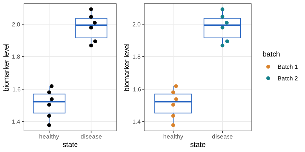
Question 13.5. Is the difference in Figure 13.2 due to the disease or to the batch?
Answer
The data cannot say: state and batch are confounded (Filling the gap 13.7 shows that only their sum is estimable). Confounding can also be biological: the biomarker may track a lifestyle that causes the disease, or an inflammation that the disease causes along with many other things.
Filling the gap 13.7: confounding is non-identifiability, and balance removes omitted-variable bias Section 13.4.1, Figure 13.2
Derivation
Complete confounding. Fit \(y=\beta_0+\beta_s s+\beta_b b+\varepsilon\) with indicators \(s\) (disease) and \(b\) (batch 2). In Figure 13.2, \(s_i=b_i\) for every sample, so the design matrix \(\mathbf{X}=[\one,\mathbf{s},\mathbf{b}]\) has two equal columns and rank 2. Then \(\mathbf{X}(\beta_0,\beta_s,\beta_b)^\T\) depends on \((\beta_s,\beta_b)\) only through \(\beta_s+\beta_b\): every pair with the same sum gives the same distribution of the data, so no estimator, however clever, can recover \(\beta_s\) separately. The least-squares normal equations \(\mathbf{X}^\T\mathbf{X}\beta=\mathbf{X}^\T y\) have a line of solutions in the direction \((0,1,-1)\). (R reports the batch coefficient as NA; qr(model.matrix(~ states + batch))$rank is 2.)
Partial confounding: the omitted-variable bias. Suppose \(b\) is not recorded and we regress \(y\) on \((\one,\mathbf{s})\) only. Conditionally on the design, the least-squares slope has expectation
\[ \E\hat\beta_s=\beta_s+\beta_b\,\frac{\widehat{\Cov}(s,b)}{\widehat{\Var}(s)}, \tag{13.e} \]with sample covariance and variance over the units. Proof: with \(\mathbf{X}_1=[\one,\mathbf{s}]\), \(\E\hat\beta=(\mathbf{X}_1^\T\mathbf{X}_1)^{-1}\mathbf{X}_1^\T(\mathbf{X}_1\beta_{(1)}+\beta_b\mathbf{b})\)
Balance. If the nuisance factor is balanced with the treatment (every state measured equally often in every batch), then \(\widehat{\Cov}(s,b)=0\) and the bias vanishes even though \(b\) was ignored; including \(b\) as a blocking factor then also removes its variance from the error (Section 13.4.4). Randomisation makes \(\widehat{\Cov}(s,b)\) zero on average for every nuisance factor, recorded or not (Filling the gap 13.12). ∎
Confounding is why Ibn Sina's rules of experimentation (around 1020, as recalled by Stigler, 2016) asked to study one possible cause at a time; Section 13.4.3 shows why Fisher could relax this rule.
13.4.2 Effect size and replicates
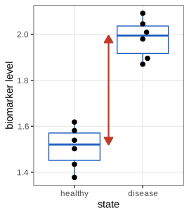
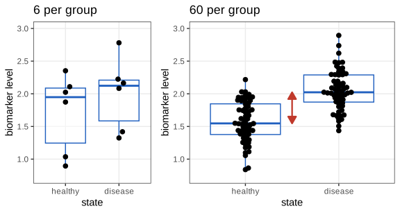
Section 13.4.2 The effect size is the distance between the group centres (Figure 13.4). More replicates locate the centres more precisely and so increase the power to detect a difference (Figure 13.5); they do not improve the biomarker's ability to classify an individual sample, which depends on how much the two distributions overlap.
Filling the gap 13.8: precision of the effect grows like \(\sqrt n\), classification accuracy does not Section 13.4.2, Figures 13.4 and 13.5
Derivation
Precision. Let both groups be normal with standard deviation \(\sigma\), centres \(\mu_0\), \(\mu_1\), \(\Delta=\mu_1-\mu_0\), and \(n\) samples each. The difference of sample means has standard error \(\sigma\sqrt{2/n}\). The sample median of \(n\) draws from a density \(f\) with median \(m\) is asymptotically normal with variance \(1/(4nf(m)^2)\) (a standard consequence of the Bahadur representation of sample quantiles); for the normal, \(f(m)=1/(\sigma\sqrt{2\pi})\), giving
\[ \Var(\text{median})\approx\frac{\pi\sigma^2}{2n}, \]so the difference of medians has standard error \(\sigma\sqrt{\pi/n}\), larger than that of the means by \(\sqrt{\pi/2}=1.25\) (simulation with \(n=61\): ratio 1.00 to within 1%). Either way the effect estimate sharpens as \(n^{-1/2}\), and the power of a test of \(\Delta=0\) tends to 1.
Classification. To assign one new sample to a group, the best rule for equal prevalences and equal variances thresholds at \((\mu_0+\mu_1)/2\), and its error probability is the Bayes error
\[ \P(\text{error})=\Phi\Big(-\frac{\Delta}{2\sigma}\Big), \]since a healthy sample is misclassified when \(X-\mu_0>\Delta/2\). This depends on \(\Delta/\sigma\) only, not on \(n\): replication tells us the threshold more precisely but cannot reduce the overlap of the populations. For the 60-per-group data of Figure 13.5 (\(\Delta\approx0.5\), \(\sigma\approx0.3\)) the Bayes error is 0.20, and the midpoint-of-medians rule misclassifies 23% of the 120 samples. With unequal prevalences the optimal threshold shifts by \(\frac{\sigma^2}{\Delta}\ln\frac{\pi_0}{\pi_1}\), and the error depends on the prevalences, as the book notes. ∎
13.4.3 Clever combinations: Hotelling's weighing example
Section 13.4.3 Eight objects with unknown weights \(\theta=(\theta_1,\dots,\theta_8)\) are to be weighed with eight uses of a two-pan balance whose readings have independent \(\N(0,\sigma^2)\) errors, \(\sigma=0.1\) (an example due to Yates and developed by Hotelling, 1944, and Mood, 1946). Method 1 weighs each object alone. Method 2 uses the rows of an \(8\times8\) matrix \(C\) of \(\pm1\) entries: in weighing \(j\) the objects with \(C_{ji}=+1\) go on the left pan and those with \(-1\) on the right, so the reading is \(y_j=\sum_iC_{ji}\theta_i+\varepsilon_j\).
Definition 13.3 (weighing design, Hadamard matrix) Section 13.4.3; Question 13.6
A weighing design is a matrix \(C\in\R^{n\times p}\) (rows weighings, columns objects) with \(|C_{ji}|\le1\); the model is \(y=C\theta+\varepsilon\), \(\varepsilon\sim\N(0,\sigma^2\I_n)\). A Hadamard matrix of order \(n\) has entries \(\pm1\) and \(H^\T H=n\I\). Sylvester's construction \(H_1=(1)\), \(H_{2k}=\begin{pmatrix}H_k&H_k\\H_k&-H_k\end{pmatrix}\) gives orders \(1,2,4,8,\dots\); its \(8\times8\) member is exactly the book's 2*hadamard(6)-1 from the survey package, and it is symmetric.
Question 13.6. Check that the design matrix is orthogonal up to a factor, and that multiplying \(\theta\) by \(C\) and then by \(C^\T\) and dividing by 8 returns \(\theta\).
Answer
By induction on Sylvester's construction, \(H_{2k}^\T H_{2k}=\begin{pmatrix}2H_k^\T H_k&0\\0&2H_k^\T H_k\end{pmatrix}\), so \(H_8^\T H_8=8\I\) (the off-diagonal blocks are \(H_k^\T H_k-H_k^\T H_k=0\)). Then \(C^\T C\theta/8=\theta\). Numerically \(C^\T C-8\I\) is exactly zero. Because \(C\) is symmetric, the book's theta %*% coef8 and coef8 %*% theta coincide; for a non-symmetric design they would not.
Filling the gap 13.9: why the Hadamard design is 8 times better, and what "8 times" means Section 13.4.3; Question 13.7, Figure 13.7
Derivation
Estimator. For any design of full column rank, least squares gives \(\hat\theta=(C^\T C)^{-1}C^\T y\), unbiased with \(\Cov\hat\theta=\sigma^2(C^\T C)^{-1}\). For the Hadamard design \(\hat\theta=C^\T y/8\) and \(\Cov\hat\theta=\frac{\sigma^2}8\I\): each weight is estimated with variance \(\sigma^2/8\), against \(\sigma^2\) for method 1, with the same number of weighings.
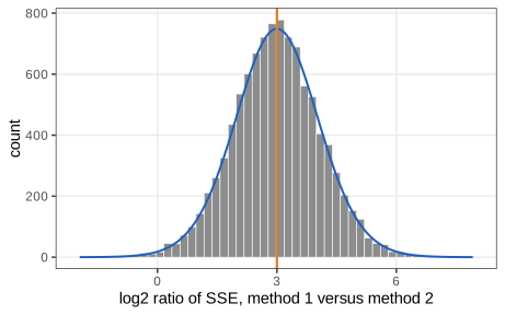
Sums of squared errors. Method 1: \(\text{SSE}_1=\sum_i\varepsilon_i^2=\sigma^2\chi^2_8\), mean \(8\sigma^2=0.08\). Method 2: \(\hat\theta-\theta=C^\T\varepsilon'/8\) is \(\N(0,\frac{\sigma^2}8\I)\), so \(\text{SSE}_2=\frac{\sigma^2}8\chi^2_8\), mean \(\sigma^2=0.01\). The book's 10 000 repetitions give 0.0795 and 0.00995. Neither depends on \(\theta\).
The ratio. The two error vectors are independent, so
\[ \frac{\text{SSE}_1}{\text{SSE}_2}=8\cdot\frac{\chi^2_8/8}{\chi'^2_8/8}=8F,\qquad F\sim F(8,8). \tag{13.f} \]Hence \(\log_2(\text{SSE}_1/\text{SSE}_2)=3+\log_2F\), whose density is drawn over the histogram in Figure 13.7. Since \(F\) and \(1/F\) have the same distribution when the degrees of freedom are equal, the median of \(F\) is 1 and the histogram is centred at \(\log_28=3\). But the mean of the ratio is \(8\E F=8\cdot\frac{8}{8-2}=\frac{32}3\approx10.7\): "8 times" is the ratio of the expected errors and the median of the ratio, not the expected ratio (simulation: median 7.96, mean 10.63). ∎
Result 13.5 (Hotelling's bound: no weighing design beats \(\sigma^2/n\)) Section 13.4.3; Hotelling (1944)
For any weighing design \(C\in[-1,1]^{n\times p}\) of full column rank and every object \(i\),
\[ \Var(\hat\theta_i)=\sigma^2\big[(C^\T C)^{-1}\big]_{ii}\ \ge\ \frac{\sigma^2}{(C^\T C)_{ii}}\ \ge\ \frac{\sigma^2}{n}, \]with equality for every \(i\) if and only if every entry is \(\pm1\) and the columns of \(C\) are orthogonal, i.e. \(C^\T C=n\I\). A Hadamard matrix is therefore optimal for every object simultaneously.
Proof
Let \(A=C^\T C\), positive definite, and \(e_i\) the \(i\)th unit vector. By the Cauchy-Schwarz inequality in the form \((u^\T v)^2\le(u^\T u)(v^\T v)\) with \(u=A^{1/2}e_i\) and \(v=A^{-1/2}e_i\),
\[ 1=(e_i^\T e_i)^2=(u^\T v)^2\le(e_i^\T Ae_i)(e_i^\T A^{-1}e_i)=A_{ii}\,[A^{-1}]_{ii}, \]which is the first inequality. Equality holds iff \(u\) and \(v\) are parallel, i.e. \(Ae_i=\lambda e_i\): \(e_i\) is an eigenvector of \(A\), meaning column \(i\) is orthogonal to all other columns. Second, \(A_{ii}=\sum_jC_{ji}^2\le n\) because \(|C_{ji}|\le1\), with equality iff every \(C_{ji}=\pm1\). Both equalities for all \(i\) mean \(A=n\I\). (Over 1413 random nonsingular \(\pm1\) designs of order 8, no variance factor fell below \(1/8\).) ∎
Spring balances. A spring balance cannot subtract, so its designs have entries in \(\{0,1\}\). For 7 objects and 7 weighings the best such design is the S-matrix obtained from \(H_8\) by deleting its first row and column and mapping \(+1\mapsto0\), \(-1\mapsto1\); it weighs four objects at a time, and \([(S^\T S)^{-1}]_{ii}=4n/(n+1)^2=7/16\) for \(n=7\) (checked exactly). The gain over one-at-a-time weighing is \(16/7\approx2.3\), not 7: being able to put objects on both pans is what makes Hotelling's design so efficient. Hotelling's design contradicts Ibn Sina's one-cause-at-a-time rule, and Fisher's factorial designs exploit the same idea: vary many factors together, with contrasts chosen so that the effects can be separated.
Question 13.7. Repeat the experiment 10 000 times with new weights each time and compare the sums of squared errors of the two methods.
Answer
The R function weighing_sse in ch13_experimental_design.R does this; the averages are close to 0.08 and 0.01, and the ratio of variances is 8 (Filling the gap 13.9). The distribution of the ratio is \(8F(8,8)\) (Figure 13.7).
13.4.4 Blocking and pairing
Section 13.4.4 Figure 13.8 shows the same kind of comparison where the measurements also depend on the time of collection. Comparing the groups within each time (a block) removes that variation from the comparison; a paired design is the simplest case of blocking.
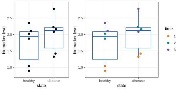
Darwin compared maize (Zea mays) plants grown from cross- and self-fertilised seed, planting the two kinds side by side in the same pots so that soil and moisture would affect both alike: each pot is a block, and the fertilisation method is the treatment. Fisher (1935) criticised that the crossed plant was always on the same side of the pot, which could confound a side effect (more light) with the treatment; the side should have been chosen by a coin flip. Block what you can, randomise what you cannot (Box et al., 1978).
Note on the data. The book describes "one seedling of each type in each of 15 pots". Darwin's data as tabulated by Fisher (1935) have 15 pairs grown in only 4 pots, with 3, 3, 5 and 4 pairs (HistData::ZeaMays, column pot); the pairs, not the pots, are the blocks of the paired analysis.
Result 13.6 (variance of a paired and of an unpaired difference) Section 13.4.4
Let \((X_i,Y_i)\), \(i=1,\dots,n\), be independent pairs with \(\Var X_i=\Var Y_i=\tau^2\) and within-pair correlation \(\rho\). Then
\[ \Var(\bar X-\bar Y)=\frac{2\tau^2(1-\rho)}{n}, \tag{13.g} \]against \(2\tau^2/n\) for two independent samples of size \(n\). Pairing divides the variance by \(1/(1-\rho)\) when \(\rho>0\), is neutral when \(\rho=0\) and harmful when \(\rho<0\). In the pot model \(X_i=P_i+\delta+\varepsilon_i\), \(Y_i=P_i+\varepsilon'_i\) with pot effects of variance \(\sigma_P^2\) and noise \(\sigma^2\), \(\tau^2=\sigma_P^2+\sigma^2\), \(\rho=\sigma_P^2/(\sigma_P^2+\sigma^2)\), and (13.g) equals \(2\sigma^2/n\): the pot effects cancel exactly.
Proof
\(\Var(X_i-Y_i)=\tau^2+\tau^2-2\rho\tau^2\), and \(\bar X-\bar Y\) is the mean of \(n\) independent differences. In the pot model \(X_i-Y_i=\delta+\varepsilon_i-\varepsilon'_i\) has variance \(2\sigma^2=2\tau^2(1-\rho)\). (Simulation with \(\rho=0.6\), \(n=15\): agreement to \(5\times10^{-5}\).) ∎
In the book's simulation \(n=15\), \(\delta=0.2\), pot effects with sd 1 and noise with sd 0.25, so \(\rho=1/1.0625=0.94\).
Question 13.8. Run an unpaired and a paired \(t\)-test on one simulated data set. Which is more powerful?
Answer
The paired test: in the book's run \(p=0.008\) for the paired test against \(p=0.57\) for the Welch test. Questions 13.9 and 13.10 show that this is the rule, not luck.
Filling the gap 13.10: the unpaired test on paired data is conservative, and the exact power of the paired test Questions 13.9 and 13.10, Figure 13.10
Derivation
The paired test. The differences \(D_i=X_i-Y_i\) are i.i.d. \(\N(\delta,2\sigma^2)\), so \(T=\bar D/(s_D/\sqrt n)\) has the noncentral \(t\) distribution with \(n-1\) degrees of freedom and noncentrality \(\lambda=\sqrt n\,\delta/(\sigma\sqrt2)\) (Result 13.7). Its power does not involve \(\sigma_P\) at all. For the book's setting \(\lambda=\sqrt{15}\cdot0.5657\), and the exact power is 0.5318. The book's simulated powers 0.555, 0.516, 0.531 and 0.563 (Questions 13.9 and 13.10, for \(\sigma_P=1,0.5,0.25,0.1\)) are all Monte Carlo estimates of this one number, with standard error 0.016.
The Welch test applied to the same pairs. Its numerator \(\bar X-\bar Y\) has variance \(2\tau^2(1-\rho)/n\) by (13.g), but its denominator estimates \((s_X^2+s_Y^2)/n\), with expectation \(2\tau^2/n\), because each sample variance sees the pot effects. For large \(n\) the denominator is close to \(\sqrt{2\tau^2/n}\), so
\[ T_{\text{W}}\approx\frac{\bar X-\bar Y}{\sqrt{2\tau^2/n}}\sim\N\big(\lambda_u,\,1-\rho\big),\qquad\lambda_u=\frac{\sqrt n\,\delta}{\tau\sqrt2}, \]and its rejection probability at level \(\alpha\) is approximately
\[ \Phi\Big(\frac{\lambda_u-z_{1-\alpha/2}}{\sqrt{1-\rho}}\Big)+\Phi\Big(\frac{-\lambda_u-z_{1-\alpha/2}}{\sqrt{1-\rho}}\Big). \tag{13.h} \]Under the null (\(\lambda_u=0\)) this is \(2\Phi(-z_{1-\alpha/2}/\sqrt{1-\rho})<\alpha\) for \(\rho>0\): the test is conservative, and its p-values pile up towards 1 (Figure 13.10). With \(\rho=0.94\) its size is \(2\Phi(-1.96/0.24)\approx10^{-16}\), and its power at \(\delta=0.2\) is essentially 0 (book: 0.001; 4000 simulations: no rejection under the null). For \(n=100\) and both standard deviations 0.5 (\(\rho=\frac12\)), (13.h) gives 0.523 (simulation 0.516; the book reports 0.508), against 0.7998 for the paired test.
What drives the difference. Larger pot effects do not help the paired test; they hurt the unpaired one. The book's conclusion that "if the pot effects are large, pairing makes a big difference" is right, but the mechanism is the degradation of the unpaired analysis. A design with independent pots would have noise variance \(2\tau^2/n\) and the ordinary two-sample power, which is the "independent pots" curve of the demo. ∎
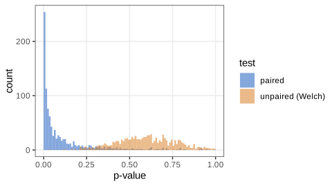
Question 13.9. Repeat the simulation 1000 times and estimate the rejection rate of each test at \(\alpha=0.05\).
Answer
The book obtains 0.001 (unpaired) and 0.555 (paired); our run behind Figure 13.10 gives 0.001 and 0.548. The exact values are 0.5318 for the paired test and essentially 0 for the Welch test (Filling the gap 13.10).
Question 13.10. Write a function comparing the power of the two tests as effect size, \(n\), pot sd and noise sd vary. Which standard deviation matters most for the benefit of pairing at \(n=15\)? How large must \(n\) be for 80% power when both standard deviations are 0.5?
Answer
The function is paired_sim in the chapter's R script (and the demo). The pot sd determines the benefit: it does not enter the paired test's power, and it makes the unpaired test conservative through \(\rho=\sigma_P^2/(\sigma_P^2+\sigma^2)\). The noise sd sets the power of the paired test itself. With both sds 0.5 the paired effect size is \(d_z=0.2/(0.5\sqrt2)=0.283\), and solving the exact power equation gives \(n=100.05\), so 101 pairs (the book's simulation at \(n=100\) gives 0.794; the exact power at 100 is 0.7998).
Filling the gap 13.11: Fisher's randomisation test for Darwin's data is exact Section 13.4.4, Fisher's criticism
Derivation
Sharp null hypothesis. Suppose that within each pair the side (or label) was assigned by a fair coin, and that crossing has no effect on any plant. Then the pair difference \(D_i\) would have been \(-D_i\) had the coin fallen the other way, so under the null the observed vector \((D_1,\dots,D_n)\) is one of \(2^n\) equally likely sign patterns \((\pm|D_1|,\dots,\pm|D_n|)\).
Test. Take the statistic \(S=|\sum_iD_i|\) and the p-value \(p=\#\{\text{sign patterns with }S'\ge S_{\text{obs}}\}/2^n\).
Exactness. Under the null, \(S_{\text{obs}}\) is uniformly distributed over the multiset \(\{S'_1,\dots,S'_{2^n}\}\) of values generated by the sign patterns. For any \(\alpha\), the patterns with \(p\le\alpha\) are those whose statistic is among the largest \(k\) values, where \(k\) is the largest number of tied-or-larger values not exceeding \(\alpha2^n\); hence \(\P(p\le\alpha)\le\alpha\), with equality when \(\alpha2^n\) falls at a gap between distinct values. No distributional assumption is used. (An exhaustive check over the 252 assignments of 10 units to two groups of 5 gives \(\P(p\le0.05)=0.048\) and \(\P(p\le0.1)=0.095\).)
Darwin's data. For the 15 differences (mean 2.62 inches) exactly 1726 of the \(2^{15}=32\,768\) sign patterns give \(|\sum\pm D_i|\ge|\sum D_i|\), so \(p=0.0527\), the value Fisher (1935) computed by hand; the paired \(t\)-test gives \(t=2.148\), \(p=0.0497\). The Welch test gives \(t=2.437\), \(p=0.023\): for these data the within-pair correlation is \(-0.33\), so by (13.g) pairing increases the variance, and the paired analysis is the less significant one. ∎
Question 13.11. What can be done when no natural pairing exists?
Answer
Matched designs build pairs of subjects that are as similar as possible (age, sex, health) and treat one of each pair. More generally a balanced design has the same number of replicates for every combination of factor levels, which keeps every factor's effect identifiable and makes nuisance factors orthogonal to the factors of interest (Filling the gap 13.7). When balance is impractical the analysis must model the imbalance explicitly, with caution.
Randomisation
When the important nuisance factors are unknown, or cannot be planned for, assign treatments at random: in large samples their effects average out. Randomisation also protects against unconscious bias, such as handling the scarce samples of one group with extra care (Senn, 2004, discusses the pitfalls of trying to improve on simple randomisation). The sense in which randomisation "averages out" nuisance factors is exact.
Filling the gap 13.12: randomisation makes the comparison unbiased, whatever the nuisance factors (Neyman, 1923) Section 13.4.4, "Randomization"
Derivation
Setting. \(N\) fixed units have fixed potential outcomes \(y_i(0)\), \(y_i(1)\) (which may depend on any nuisance property of the unit, measured or not). A completely randomised design picks \(n_1\) units for treatment uniformly among the \(\binom N{n_1}\) subsets; the rest (\(n_0=N-n_1\)) are controls. The estimator is \(\hat\tau=\bar y_1^{\text{obs}}-\bar y_0^{\text{obs}}\), and the target the average effect \(\tau=\frac1N\sum_i(y_i(1)-y_i(0))\).
Unbiasedness. With \(W_i\) the treatment indicator, \(\P(W_i=1)=n_1/N\), so \(\E\bar y_1^{\text{obs}}=\frac1{n_1}\sum_i\E[W_i]y_i(1)=\bar y(1)\), and likewise \(\E\bar y_0^{\text{obs}}=\bar y(0)\). Hence \(\E\hat\tau=\tau\), the expectation being over the randomisation only: no model for the outcomes is assumed.
Variance. Using \(\Var W_i=\frac{n_1n_0}{N^2}\) and \(\Cov(W_i,W_j)=-\frac{n_1n_0}{N^2(N-1)}\) for \(i\ne j\) (sampling without replacement), a direct computation gives
\[ \Var\hat\tau=\frac{S_1^2}{n_1}+\frac{S_0^2}{n_0}-\frac{S_\tau^2}{N}, \tag{13.i} \]where \(S_1^2\), \(S_0^2\), \(S_\tau^2\) are the finite-population variances (divisor \(N-1\)) of \(y_i(1)\), \(y_i(0)\) and \(y_i(1)-y_i(0)\). The usual estimate \(s_1^2/n_1+s_0^2/n_0\) is unbiased for the first two terms and so conservative. For a balanced covariate, the imbalance \(\bar x_1-\bar x_0\) has mean 0 and variance \(S_x^2(1/n_1+1/n_0)\): any nuisance factor is balanced on average and its chance imbalance shrinks like \(N^{-1/2}\).
Check. Enumerating all 252 assignments of 10 units with heterogeneous effects reproduces \(\E\hat\tau=\tau\) and (13.i) to machine precision. The same randomisation distribution, with the outcomes held fixed under the sharp null, gives the exact test of Filling the gap 13.11. ∎
13.4.5 How many replicates do I need?
Section 13.4.5 A cell-line experiment may give the right answer with one replicate (we do two or three to be safe); a comparison of two drugs in patients may need dozens or hundreds, because uncontrolled variability is so much larger. The number depends on that variability and on the effect size, which is the "elephant in the room" of power calculations (Figure 13.11 of the book, a photograph not reproduced here): in screens of thousands of features we rarely know it. Power calculations are still useful for orders of magnitude and for comparing designs. Four quantities are linked: sample size, effect size, level \(\alpha\) and power; the R package pwr solves for any one of them (pwr.t.test, pwr.2p.test, pwr.chisq.test, pwr.f2.test).
Definition 13.4 (noncentral \(t\) distribution)
If \(Z\sim\N(0,1)\) and \(V\sim\chi^2_\nu\) are independent and \(\lambda\in\R\), then \(T=(Z+\lambda)/\sqrt{V/\nu}\) has the noncentral \(t\) distribution \(t_\nu(\lambda)\). Conditioning on \(W=\sqrt V\),
\[ \P(T>c)=\int_0^\infty\Big[1-\Phi\Big(\frac{cw}{\sqrt\nu}-\lambda\Big)\Big]f_W(w)\,\d w,\qquad f_W(w)=\frac{2^{1-\nu/2}w^{\nu-1}e^{-w^2/2}}{\Gamma(\nu/2)}, \]a one-dimensional integral (this is how the demonstrations compute it; R's pt(q, df, ncp) uses a series).
Result 13.7 (exact power of the \(t\)-tests) Section 13.4.5, pwr.t.test
(a) One sample or \(n\) pairs. For i.i.d. \(\N(\mu,\sigma^2)\) observations (the pair differences) and \(H_0:\mu=0\), the statistic \(T=\bar X/(s/\sqrt n)\) is \(t_{n-1}(\lambda)\) with \(\lambda=\sqrt n\,d\), \(d=\mu/\sigma\). (b) Two groups of \(n\) with common \(\sigma\) and the pooled-variance statistic, \(T\sim t_{2n-2}(\lambda)\) with \(\lambda=\sqrt{n/2}\,d\), \(d=(\mu_1-\mu_2)/\sigma\). In both cases the two-sided level-\(\alpha\) test has power
\[ \beta(n,d,\alpha)=\P(T>t_{1-\alpha/2,\nu})+\P(T<-t_{1-\alpha/2,\nu}),\qquad T\sim t_\nu(\lambda). \tag{13.j} \]For \(n=15\), \(d=0.4\): two groups 0.1848496, paired 0.3031649; 80% power needs 99.08 per group or 51.01 pairs, exactly the book's pwr.t.test output.
Proof
(a) For normal samples \(\bar X\) and \(s^2\) are independent, \(\sqrt n(\bar X-\mu)/\sigma\sim\N(0,1)\) and \((n-1)s^2/\sigma^2\sim\chi^2_{n-1}\) (the classical theorem behind Student's \(t\), proved by an orthogonal change of variables that puts \(\sqrt n\bar X\) in the first coordinate). Write
\[ T=\frac{\sqrt n\bar X/\sigma}{s/\sigma}=\frac{Z+\sqrt n\mu/\sigma}{\sqrt{V/(n-1)}},\quad Z=\frac{\sqrt n(\bar X-\mu)}\sigma,\ V=\frac{(n-1)s^2}{\sigma^2}, \]which is Definition 13.4 with \(\lambda=\sqrt nd\). (b) \(\bar X_1-\bar X_2\sim\N(\mu_1-\mu_2,2\sigma^2/n)\), independent of the pooled variance \(s_p^2\) with \((2n-2)s_p^2/\sigma^2\sim\chi^2_{2n-2}\); dividing by \(s_p\sqrt{2/n}\) gives \(\lambda=(\mu_1-\mu_2)/(\sigma\sqrt{2/n})=\sqrt{n/2}\,d\). The test rejects when \(|T|>t_{1-\alpha/2,\nu}\), which is (13.j). pwr.t.test evaluates exactly this with pt(..., ncp) and solves for \(n\) on a continuous scale; our implementation agrees with it to \(10^{-15}\), with power.t.test(strict = TRUE), and with 20 000 simulated two-sample tests (0.1846). ∎
Filling the gap 13.13: the normal-approximation sample size and its correction
Derivation
Known \(\sigma\). If \(\sigma\) were known, the statistic would be \(\N(\lambda,1)\) and the two-sided power \(\Phi(\lambda-z_{1-\alpha/2})+\Phi(-\lambda-z_{1-\alpha/2})\). The second term is the probability of rejecting in the wrong direction and is negligible once the power is substantial (below \(\alpha/2\) whenever \(\lambda>0\)). Setting \(\Phi(\lambda-z_{1-\alpha/2})=1-\beta\) gives \(\lambda=z_{1-\alpha/2}+z_{1-\beta}\), and with \(\lambda=\sqrt nd\) or \(\sqrt{n/2}\,d\):
\[ n_{\text{pairs}}\approx\frac{(z_{1-\alpha/2}+z_{1-\beta})^2}{d^2},\qquad n_{\text{per group}}\approx\frac{2(z_{1-\alpha/2}+z_{1-\beta})^2}{d^2}. \tag{13.k} \]For \(\alpha=0.05\), power 0.8, \(d=0.4\): 49.06 pairs and 98.11 per group.
Why it is too small. Estimating \(\sigma\) adds variability: \(T=(Z+\lambda)/W'\) with \(W'=\sqrt{V/\nu}\) has heavier tails than the normal, and the critical value \(t_{1-\alpha/2,\nu}\) exceeds \(z_{1-\alpha/2}\). A first-order expansion, \(W'\approx1+\xi/\sqrt{2\nu}\) with \(\xi\sim\N(0,1)\), shows \(T>c\) iff approximately \(Z-c\xi/\sqrt{2\nu}>c-\lambda\), where the left side has variance \(1+c^2/(2\nu)\); the required \(\lambda\) therefore grows by a term of order \(1/\nu\), i.e. \(n\) grows by a constant. Guenther (1981) gives the practical correction
\[ n_{\text{pairs}}\approx(13.\text{k})+\frac{z_{1-\alpha/2}^2}2,\qquad n_{\text{per group}}\approx(13.\text{k})+\frac{z_{1-\alpha/2}^2}4, \]which gives 50.98 and 99.07 against the exact 51.01 and 99.08. (The correction is checked numerically to within 0.1, not derived here in full.) ∎
Filling the gap 13.14: what "about twice as many observations without pairing" assumes Section 13.4.5, pwr.t.test with type = "paired"
Derivation
The book computes 99.08 per group for the two-sample test and 51.01 pairs for the paired test, both with \(d=0.4\), and concludes that about twice as many observations are needed without pairing. But the two \(d\)'s are on different scales: for the paired test \(d_z=\delta/\sigma_D\), the mean difference over the sd of the differences, while for the two-sample test \(d=\delta/\tau\). By (13.g), \(\sigma_D=\tau\sqrt{2(1-\rho)}\), so
\[ d_z=\frac{d}{\sqrt{2(1-\rho)}}. \]Using the same number for both means \(2(1-\rho)=1\), \(\rho=\frac12\). With (13.k), \(n_{\text{pairs}}/n_{\text{per group}}\approx\frac{d^2}{2d_z^2}=1-\rho\): the paired design needs \(1-\rho\) times as many pairs as the unpaired design needs subjects per group, and so \(1-\rho\) times as many observations. The factor 2 is the case \(\rho=\frac12\). With \(\rho=0\) (no real pairing) the paired analysis needs 100.05 pairs against 99.08 per group, slightly more, because it has \(n-1\) instead of \(2n-2\) degrees of freedom; with \(\rho<0\), as in Darwin's data, it needs considerably more. ∎
Effective sample size
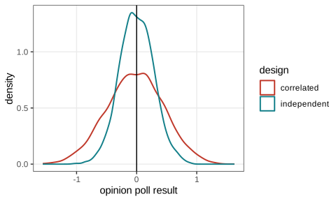
Independent observations are more informative than the same number of dependent ones. The book's opinion poll asks 12 of 100 people, either at 12 random doors or at 4 random doors and their two neighbours, on a street where opinions are sorted from most negative to most positive, so that neighbours think alike.
Result 13.8 (variance of a mean of correlated observations; design effect)
(a) For \(X_1,\dots,X_n\) with common variance \(\sigma^2\) and correlations \(\rho_{ij}\), \(\Var\bar X=\frac{\sigma^2}{n^2}\sum_{i,j}\rho_{ij}\). (b) If the observations form \(k\) clusters of \(m\) (\(n=km\)), with correlation \(\rho\) within clusters and 0 between,
\[ \Var\bar X=\frac{\sigma^2}{n}\,\big[1+(m-1)\rho\big],\qquad n_{\text{eff}}=\frac{n}{1+(m-1)\rho}. \tag{13.l} \]The factor \(\deff=1+(m-1)\rho\) is the design effect (Kish, 1965); \(n_{\text{eff}}\) independent observations give the same precision. For \(\rho\to1\), \(n_{\text{eff}}\to k\): each cluster counts once.
Proof
(a) \(\Var\sum X_i=\sum_{i,j}\Cov(X_i,X_j)=\sigma^2\sum_{i,j}\rho_{ij}\). (b) The double sum has \(n\) diagonal terms equal to 1 and, in each of the \(k\) clusters, \(m(m-1)\) off-diagonal terms equal to \(\rho\): \(n+km(m-1)\rho=n[1+(m-1)\rho]\). Simulation with \(m=3\), \(k=4\), \(\rho=\frac12\): agreement to \(10^{-4}\). ∎
Filling the gap 13.15: the exact spread of the two polls of Figure 13.12 Section 13.4.5, doPoll
Derivation
Random doors. The 100 opinions are i.i.d. \(\N(0,1)\) and then sorted along the street; the 12 doors are chosen independently of the opinions. A uniformly random subset of exchangeable variables is distributed like any fixed subset, so the 12 answers are i.i.d. \(\N(0,1)\) and the poll mean is exactly \(\N(0,1/12)\), variance 0.0833, regardless of the sorting.
Groups of neighbours. The code's groups are houses \((3g-2,3g-1,3g)\), \(g=1,\dots,33\), with group means \(T_g\); 4 of the 33 groups are chosen without replacement. Conditionally on the street, the poll is the mean of a simple random sample of 4 out of 33 values, with mean \(\bar T\) and variance \(\frac{S_T^2}{4}(1-\frac4{33})\) (the finite-population correction). By the law of total variance,
\[ \Var(\text{poll})=\E\Big[\frac{S_T^2}{4}\Big(1-\frac4{33}\Big)\Big]+\Var(\bar T). \]Simulation of 40 000 streets gives a variance of 0.218 (the two-stage formula agrees within 1.2%), so the design effect is \(0.218/0.0833=2.6\) and the 12 answers are worth about \(n_{\text{eff}}=4.6\) independent ones: almost one per group, since sorted neighbours are nearly identical (\(\rho\approx0.8\) in (13.l)).
A small bias in the book's code. Groups end at houses \(3,6,\dots,99\), so house 100, which holds the largest opinion, is never polled. The groups' poll is then an average over the 99 lowest order statistics, whose expected mean is \(-\E X_{(100)}/99=-2.5076/99=-0.0253\) (since all 100 sum to mean 0). The simulated mean is \(-0.0253\). The effect is small next to the spread, but it is a reminder that a sampling frame that silently excludes units creates bias. ∎
13.5 Mean-variance relationships and variance-stabilizing transformations
Section 13.5 The mixture-model and count-data chapters transformed data so that the variance between replicates no longer depends strongly on their mean. Before transformation, the variance \(v\) as a function of the mean \(m\) is often close to one of three prototypes, with constants \(a,b,c\ge0\): constant, \(v(m)=c\); Poisson-like, \(v(m)=am\); quadratic (constant coefficient of variation), \(v(m)=bm^2\). Microarray intensities combine additive background noise and multiplicative noise, \(v(m)=bm^2+c\) (Rocke and Durbin, 2001): multiplicative noise dominates for bright spots and background for faint ones.
Filling the gap 13.16: the variance-stabilising transformation for each mean-variance relationship Section 13.5
Derivation
Principle. Let \(X\) have mean \(m\) and variance \(v(m)\), and let \(g\) be smooth. A first-order Taylor expansion \(g(X)\approx g(m)+g'(m)(X-m)\) (the delta method, accurate when the spread of \(X\) is small on the scale on which \(g'\) changes) gives \(\Var g(X)\approx g'(m)^2v(m)\). Requiring this to equal 1 for every \(m\) gives the differential equation \(g'(m)=v(m)^{-1/2}\), so
\[ g(m)=\int^m\frac{\d u}{\sqrt{v(u)}}. \tag{13.m} \]The prototypes. \(v=c\): \(g(m)=m/\sqrt c\), no transformation. \(v=am\): \(g(m)=2\sqrt{m/a}\), the square root. \(v=bm^2\): \(g(m)=\ln(m)/\sqrt b\), the logarithm.
Additive plus multiplicative noise, \(v=bm^2+c\). Substituting \(u=\sqrt{c/b}\sinh t\) gives \(\sqrt{bu^2+c}=\sqrt c\cosh t\) and \(\d u=\sqrt{c/b}\cosh t\,\d t\), so
\[ g(m)=\frac1{\sqrt b}\arsinh\Big(m\sqrt{\tfrac bc}\Big),\qquad \arsinh(x)=\ln\big(x+\sqrt{x^2+1}\big). \]It is linear near 0 (\(g\approx m/\sqrt c\), where background noise dominates) and logarithmic for large \(m\) (\(g\approx\ln(2m\sqrt{b/c})/\sqrt b\)), and, unlike the logarithm, it is defined for zero and negative background-corrected values. This is the "generalised logarithm" behind vsn (Huber et al., 2002).
Negative binomial counts, \(v=m+\alpha m^2\). With \(u=\sinh^2(t)/\alpha\), \(\sqrt{u+\alpha u^2}=\sinh t\cosh t/\alpha\) and \(\d u=2\sinh t\cosh t\,\d t/\alpha\), so
\[ g(m)=\frac2{\sqrt\alpha}\arsinh\big(\sqrt{\alpha m}\big), \]which is \(2\sqrt m\) for \(\alpha m\ll1\) and \(\ln(4\alpha m)/\sqrt\alpha\) for \(\alpha m\gg1\); DESeq2's variance-stabilising transformation is built on this function.
How good is first order? Poisson with mean 50: \(\Var(2\sqrt X)=1.0077\), and Anscombe's \(2\sqrt{X+3/8}\) gives 1.00003. Additive-plus-multiplicative noise with a 10% coefficient of variation: \(\Var g(X)\) is within 2% of 1 from \(m=0\) to \(10^4\). Negative binomial with \(\mu=100\), \(\alpha=0.1\) (a 33% coefficient of variation): 1.052. The approximation degrades as the relative spread grows, because the neglected second-order term is of the order of the squared coefficient of variation. ∎
Question 13.12. Give assays whose data show each type of mean-variance relationship.
Answer
Constant: measurements dominated by additive instrument noise, such as background-level fluorescence or log-scale data that have already been stabilised. Poisson: counts of independent events, such as reads of a gene across technical replicates of a library, photon counts, colony or cell counts. Quadratic: multiplicative errors, such as bright microarray spots, ELISA or mass-spectrometry intensities at high concentration, and highly expressed genes across biological replicates, where the \(\alpha m^2\) term of the negative binomial dominates.
Question 13.13. What is the point of a variance-stabilising transformation?
Answer
On the transformed scale, plots and heatmaps use their space and colour range evenly across the dynamic range; PCA, clustering and correlations are no longer dominated by a few highly expressed features; and models that assume identically distributed (homoskedastic) noise give valid estimates and tests.
13.6 Data quality assessment and quality control
Section 13.6 Quality assessment (QA) measures and monitors data quality; quality control (QC) removes bad data. Both run through every stage of an analysis. Typical QA questions: what do the marginal distributions look like (histograms, ECDFs) and the joint ones (scatter and pairs plots)? Do replicates agree better with each other than with other conditions, and are the differences between conditions plausible? Are there batch effects, stepwise (a reagent change) or gradual (an instrument drifting), recorded or latent? Heatmaps and ordination plots (PCA and its relatives) answer the last two. The most useful notion of quality is fitness for purpose rather than conformance to specifications: read counts, read lengths and alignment rates matter less for a differential-expression study than spotting samples that do not behave as expected (a swap, degradation) or genes that were not measured properly. A quality metric is any number used to measure quality; explicit metrics make QA/QC automatable. When a metric is computed for many samples or features, its extremes need the multiple-comparison view of Filling the gap 13.19: among thousands of perfectly good samples, some will look extreme.
13.7 Longitudinal data
Section 13.7 When time is a covariate, the first question is whether we have a few time points (a cell line at 48, 72 and 96 hours) or a long, densely sampled series (patch-clamp recordings, live-cell movies). A few time points are best treated as levels of an experimental factor; one can look for the most informative one and use the others as approximate replicates, and sample densely where most is expected to happen. To ask whether there is any time effect at all one can use an \(F\)-test, provided its null distribution accounts for the dependence between measurements of the same unit.
Filling the gap 13.17: an exact \(F\)-test for a time effect with repeated measurements Section 13.7, "account for the dependencies"
Derivation
Model. Subject \(s=1,\dots,n\) is measured at times \(t=1,\dots,T\): \(y_{st}=\mu_t+S_s+\varepsilon_{st}\) with independent subject effects \(S_s\sim\N(0,\sigma_S^2)\) and noise \(\varepsilon_{st}\sim\N(0,\sigma^2)\). The vector \(\mathbf{y}_s\in\R^T\) has covariance \(\bm\Sigma=\sigma_S^2\one\one^\T+\sigma^2\I\) (compound symmetry). We test \(H_0:\mu_1=\dots=\mu_T\).
Contrasts remove the subject. Let \(Q\in\R^{T\times(T-1)}\) have orthonormal columns orthogonal to \(\one\) (normalised Helmert contrasts). Then \(\mathbf{u}_s=Q^\T\mathbf{y}_s\) has covariance \(Q^\T\bm\Sigma Q=\sigma^2\I_{T-1}\), because \(Q^\T\one=0\), and mean \(Q^\T\bm\mu\), which is 0 exactly under \(H_0\). So the \(\mathbf{u}_s\) are i.i.d. \(\N(Q^\T\bm\mu,\sigma^2\I)\).
The test. With \(\bar{\mathbf{u}}=\frac1n\sum\mathbf{u}_s\), \(n\|\bar{\mathbf{u}}\|^2/\sigma^2\sim\chi^2_{T-1}\) under \(H_0\), independent of \(\sum_s\|\mathbf{u}_s-\bar{\mathbf{u}}\|^2/\sigma^2\sim\chi^2_{(n-1)(T-1)}\), so
\[ F=\frac{n\|\bar{\mathbf{u}}\|^2/(T-1)}{\sum_s\|\mathbf{u}_s-\bar{\mathbf{u}}\|^2/\big((n-1)(T-1)\big)}\sim F\big(T-1,(n-1)(T-1)\big). \]Since \(QQ^\T=\I-\frac1T\one\one^\T\) (the centring projection), the numerator sum of squares is \(n\sum_t(\bar y_{\cdot t}-\bar y_{\cdot\cdot})^2\) and the denominator is the residual sum of squares of the two-way model "subject + time": this \(F\) is exactly the time test of lm(y ~ subject + time), with subjects as blocks.
Ignoring the subjects puts \(\sigma_S^2\) into the error and makes a one-way ANOVA very conservative (simulated size below 0.001, while the blocked test rejects close to 5% of 2000 null data sets). If the correlation decays with the time lag, compound symmetry fails and the \(F\)-test is no longer exact; then a corrected test (Greenhouse-Geisser) or a mixed model with a suitable covariance is needed. ∎
Filling the gap 13.18: regression to the mean in before-after data
Derivation
Setting. A quantity is measured twice without any intervention, \((X_1,X_2)\) bivariate normal with mean \(\mu\), standard deviation \(\sigma\) and correlation \(\rho<1\) (measurement noise or day-to-day variation makes \(\rho<1\)). Units are selected because \(X_1\) is extreme, say \(X_1>\mu+c\sigma\) (the heaviest patients, the most highly expressed genes in a pilot).
Result. \(\E[X_2\given X_1]=\mu+\rho(X_1-\mu)\), so with standardised variables
\[ \E[X_2-X_1\given X_1>\mu+c\sigma]=-(1-\rho)\,\sigma\,\frac{\varphi(c)}{1-\Phi(c)}. \tag{13.n} \]Proof: \(\E[X_2-X_1\given X_1]=-(1-\rho)(X_1-\mu)\), and for \(Z\sim\N(0,1)\), \(\E[Z\given Z>c]=\frac1{1-\Phi(c)}\int_c^\infty z\varphi(z)\d z=\frac{\varphi(c)}{1-\Phi(c)}\) because \(\varphi'(z)=-z\varphi(z)\). With \(\rho=0.6\) and \(c=1\) the selected units "improve" by \(0.61\sigma\) on average with no treatment at all (simulation agrees to 0.002).
Consequence for design. A before-after comparison on units selected for extreme baseline values confounds any treatment effect with (13.n). A randomised control group selected the same way regresses by the same amount, and the treatment effect is the difference between the groups' changes. ∎
Long, densely sampled series call for dynamical models of the state \(X(t)\), which may be continuous or discrete, deterministic or stochastic, smooth or jumpy, and observed directly or only through a lossy, noisy \(Y=g(X)+\varepsilon\). The tools include Markov models (discrete states, stochastic jumps; hidden Markov models when only \(Y\) is seen, Durbin et al., 1998), ordinary and partial differential equations (continuous, deterministic, smooth dynamics), master and Fokker-Planck equations (stochastic dynamics written as equations for the probability distribution), and piecewise-deterministic processes that combine smooth motion with occasional jumps. Data-driven alternatives are smoothing followed by clustering of the curves, change-point detection, autoregressive models, and Fourier or wavelet decompositions. (Survival data, where time is the outcome rather than a covariate, are a different topic.)
13.8 Data integration: use everything you (could) know
Section 13.8 Generic methods that treat a data matrix without reference to what its rows and columns mean are a fine start, but often wasteful. In a differential-expression screen, hypotheses differ in power (through their mean count) and in their prior probability \(\pi_0\) of being null; filtering or weighting them uses this knowledge and gains power (the multiple-testing chapter's independent filtering and IHW). Prior knowledge also helps when interpreting a single p-value (Altman and Krzywinski, 2017), when penalising features in high-dimensional regression differently by class (van de Wiel et al., 2016) or along a graph (group and graph lasso, Jacob et al., 2009), and when clustering objects measured with different precision (Callahan et al., 2016). Results should be confronted with other data: gene-set collections such as MSigDB (Liberzon et al., 2011), and data from the levels of regulation upstream and downstream.
Filling the gap 13.19: the curse of large \(p\): extremes of many null statistics Sections 13.6 and 13.8
Derivation
Claim. For \(Z_1,\dots,Z_p\sim\N(0,1)\), not necessarily independent,
\[ \E\max_{i\le p}Z_i\le\sqrt{2\ln p}. \]Proof. For any \(s>0\), by Jensen's inequality and then bounding the maximum by the sum,
\[ e^{s\E\max Z_i}\le\E e^{s\max Z_i}=\E\max_ie^{sZ_i}\le\sum_i\E e^{sZ_i}=pe^{s^2/2}, \]so \(\E\max Z_i\le\frac{\ln p}s+\frac s2\). The right side is minimal at \(s=\sqrt{2\ln p}\), where it equals \(\sqrt{2\ln p}\). For independent variables the bound is sharp to first order (\(\E\max Z_i/\sqrt{2\ln p}\to1\)). ∎
Consequences for pipelines. (i) With \(p=10^4\) null features, the largest \(z\)-score is about 3.85 on average (bound 4.29): a quality metric or test statistic that is "extreme" among thousands is not evidence by itself, which is why thresholds must account for \(p\) (Bonferroni or FDR control, the multiple-testing chapter). (ii) Winner's curse: if the feature with the largest estimated effect is selected and its effect is then reported from the same data, the estimate is biased upwards by roughly this order of magnitude times its standard error; effects of selected features should be estimated on independent data or with methods that account for the selection. (iii) Filtering before testing is valid when the filter statistic is independent of the test statistic under the null (for normal data, the overall mean or variance across both groups is independent of the two-sample \(t\)-statistic under the null, Bourgon et al., 2010); a filter that looks at the group difference is not. ∎
13.9 Sharpen your tools: reproducible research
Section 13.9 Analyses grow from a script to a project with more data, more people and, eventually, a paper whose figures and methods must be reproducible. The book's principles, in brief (see also Wilson et al., 2017): work in an integrated development environment; use literate programming (Quarto, R Markdown, Jupyter) so that code, explanation and figures live together and can become supplementary material; expect to redesign data formats and code as the project evolves, and do it as soon as manipulations become awkward; reuse tested tools before writing heuristics of your own; use version control (git) from the start; write functions instead of copying code, and move shared functions into an R package with documentation, examples and tests; keep raw data read-only in one backed-up place and derive everything else from it by a versioned, re-runnable workflow; write "recipe" scripts that assemble heterogeneous inputs into analysis-ready objects such as a SummarizedExperiment; and keep an index page linking all analyses.
13.10 Data representation
Section 13.10 Much effort goes into reshaping data for an algorithm or a plot; ggplot2 expects one row per measurement, the "tidy" format of Wickham (2014).
13.10.1 Wide vs long table format
Section 13.10.1 Taking four genes (Fgf4, Gata4, Gata6, Sox2) of the Hiiragi mouse-embryo data, a wide table has one row per gene: the probe and symbol, then 101 columns of expression values whose column names encode sample and embryonic stage (a \(4\times103\) table). tidyr::pivot_longer turns it into a long table with one row per measured value (404 rows) and columns probe, symbol, sample, value. In the wide form we must "know" which columns are covariates and which are data, and subsetting samples (columns) differs from subsetting genes (rows); in the long form every row is one observation, new covariates are new columns, new genes or samples are new rows, and every subset is one filter call. There is a second wide form (one row per sample, one column per gene), and each wide form is the natural input for some plots; pivot_wider goes back from long to wide.
13.11 Tidy data: using it wisely
Section 13.11 Tidy data put each variable in a column, each observation in a row and each type of observational unit in its own table. The long format is not a panacea. Efficiency and integrity: the four probe-to-symbol pairs are stored 404 times, nothing guarantees that the copies agree, and an update must touch them all; long tables are best assembled late from normalised containers. No contracts: nothing states what "a table like this" must contain, whereas classes (S4 in R, with validObject methods) can, along with encapsulation, polymorphism, inheritance and introspection; this is the design of Bioconductor's SummarizedExperiment. Provenance and metadata (who, where, which version, units, assay) have no obvious place in a data frame. Matrix-shaped data (features by samples) are awkward to unroll for PCA, SVD or clustering.
13.12 Leaky pipelines and statistical sufficiency
Section 13.12 High-throughput pipelines are funnels: images become base calls, reads, alignments, counts per position, counts per gene, normalised values. Each step discards information, and a pipeline assembled from separately developed parts can discard what a later step needs (differential expression needs the raw counts, not normalised values; some questions need exon- or isoform-level counts). The statistical notion that says which summaries are safe is sufficiency.
Definition 13.5 (sufficient statistic)
A statistic \(S(\mathbf{x})\) is sufficient for a parameter \(\theta\) of a model \(p(\mathbf{x}\given\theta)\) if the conditional distribution of the data given \(S\) does not depend on \(\theta\). Then everything the data say about \(\theta\) (the likelihood up to a factor free of \(\theta\)) is a function of \(S\).
Result 13.9 (factorisation criterion, discrete case)
\(S\) is sufficient if and only if \(p(\mathbf{x}\given\theta)=h(\mathbf{x})\,k(S(\mathbf{x}),\theta)\) for some functions \(h\) and \(k\).
Proof
If the factorisation holds, then for \(\mathbf{x}\) with \(S(\mathbf{x})=s\), \(\P(\mathbf{x}\given S=s,\theta)=\frac{h(\mathbf{x})k(s,\theta)}{\sum_{\mathbf{y}:S(\mathbf{y})=s}h(\mathbf{y})k(s,\theta)}=\frac{h(\mathbf{x})}{\sum_{\mathbf{y}:S(\mathbf{y})=s}h(\mathbf{y})}\), free of \(\theta\). Conversely, if \(S\) is sufficient, \(p(\mathbf{x}\given\theta)=\P(\mathbf{x}\given S=s)\,\P(S=s\given\theta)\), which is the factorisation with \(h(\mathbf{x})=\P(\mathbf{x}\given S=S(\mathbf{x}))\). ∎
Bernoulli trials. For \(n\) independent trials with success probability \(p\), \(p(\mathbf{x}\given p)=p^k(1-p)^{n-k}\) with \(k=\sum x_i\), so the number of successes is sufficient: given \(k\), each of the \(\binom nk\) arrangements has probability \(1/\binom nk\) (checked by enumeration for \(n=5\)).
Question 13.14. For a Markov chain on the four states A, C, G, T, which statistics are sufficient for the transition probabilities? (The book refers to the chain "we saw in Chapter 13"; the Markov chain model of DNA sequences is in the statistical-modelling chapter, Chapter 2.)
Answer
For a sequence \(x_1,\dots,x_L\) with initial distribution \(\pi\) and transition matrix \(P=(p_{ab})\),
\[ p(\mathbf{x}\given P)=\pi(x_1)\prod_{l=2}^{L}p_{x_{l-1}x_l}=\pi(x_1)\prod_{a,b}p_{ab}^{\,n_{ab}}, \]where \(n_{ab}\) counts the transitions from \(a\) to \(b\). By the factorisation criterion the 16 transition counts (with the first letter, if \(\pi\) is also unknown) are sufficient: the order in which the transitions occur is irrelevant. Maximising \(\sum_bn_{ab}\ln p_{ab}\) separately for each row \(a\) under \(\sum_bp_{ab}=1\) (a Lagrange multiplier gives \(n_{ab}/p_{ab}=\lambda_a\); the objective is concave) yields \(\hat p_{ab}=n_{ab}/\sum_{b'}n_{ab'}\). Both the factorisation and the maximum were checked numerically.
Filling the gap 13.20: normalised counts are not sufficient Section 13.12, footnote on raw counts
Derivation
Let a gene's count in a library of size factor \(s\) be \(K\sim\text{Poisson}(s\mu)\), and suppose the pipeline passes on only \(Y=K/s\). Two libraries with \(Y=1\), one with \((s,K)=(1,1)\) and one with \((100,100)\), have likelihoods for \(\mu\) proportional to \(\mu e^{-\mu}\) and \(\mu^{100}e^{-100\mu}\): the second pins \(\mu\) down ten times more precisely (\(\Var\hat\mu=\mu/s\)). Since the likelihood is not a function of \(Y\) alone, \(Y\) is not sufficient; the pair \((K,s)\) is. This is why count-based methods want raw counts together with size factors, and why a variance computed from normalised values misrepresents the information in each sample. Pipelines should pass on sufficient statistics, or enough to reconstruct the likelihood. ∎
Iterative schemes, in the spirit of the EM algorithm, can recover information lost in a first pass: in mass spectrometry, peaks are first called in each sample separately, and a second pass borrows strength across samples to find peaks that looked like noise in one sample alone.
13.13 Efficient computing
Section 13.13 Beware of premature optimisation: a slow solution to the right problem beats a fast solution to the wrong one, it is often best to get the analysis right on a subset first, and our own time is usually worth more than computer time. When performance does matter, R offers four tools. Vectorisation: computing \(a_i^2b_i\) for \(10^6\) elements with a single expression a^2 * b is many times faster than a for loop and gives an identical result; ifelse, dplyr::lead/lag and whole-table dplyr verbs extend the idea. Parallelisation is natural in a functional language (BiocParallel). Out-of-memory data and chunking: process data in pieces, or keep them in a database (DBI) or in HDF5 (rhdf5, or a SummarizedExperiment with an HDF5 back end). Lower-level languages: Rcpp embeds short C++ functions (wrapping R vectors as NumericVector), to be used for the time-critical parts only, with input checks.
Summary
- Error is bias plus noise; replication reduces only the noise, and correlated error behaves like bias (Result 13.1). Whether a source of variation is noise or bias is a modelling choice, and refining the groups turns within-group noise into explained variation (Filling the gap 13.2).
- Replicate at the level you want to generalise to: technical replicates reduce only \(\sigma_E^2\), the optimum number is \(\sqrt{c_B\sigma_E^2/(c_T\sigma_B^2)}\), and treating them as independent inflates false positives (Result 13.2, Filling the gap 13.4).
- Confounded factors cannot be separated by any analysis; balance and randomisation prevent the problem (Filling the gap 13.7, 13.12).
- Combining measurements cleverly can multiply precision: Hotelling's Hadamard design attains the bound \(\sigma^2/n\) for every object (Result 13.5).
- Pairing divides the variance by \(1/(1-\rho)\) and only helps for \(\rho>0\); the paired test's power depends only on the noise, and an unpaired test on paired data is conservative (Result 13.6, Filling the gap 13.10).
- Power comes from the noncentral \(t\) distribution; the normal formula \(n\approx k(z_{1-\alpha/2}+z_{1-\beta})^2/d^2\) needs a small correction (Result 13.7, Filling the gap 13.13). Correlated observations count as \(n/[1+(m-1)\rho]\) (Result 13.8).
- Variance-stabilising transformations solve \(g'=v^{-1/2}\); repeated measures need contrasts that remove the subject; selected extremes regress to the mean; extremes among \(p\) features grow like \(\sqrt{2\ln p}\); and pipelines must keep sufficient statistics.
Exercises
The six exercises of Chapter 13 (Holmes and Huber, 2019, Section 13.16), restated in my own words, with solutions (hidden). Exercises 13.4 to 13.6 are about software practice and have no single answer; their solutions outline the steps.
Exercise 13.1. Design a simulation to choose the number of subjects when the measurement noise follows a symmetric Laplace distribution (the infinite normal mixture of the mixture-model chapter). Tabulate the answer over several noise levels and effect sizes.
Solution
Simulating the noise. By Result 13.4, Laplace(\(b\)) noise is \(\N(0,V)\) with \(V\) exponential with mean \(2b^2\): draw \(V\), then a normal with that variance. Its standard deviation is \(b\sqrt2\).
Design. For each noise scale \(b\), effect \(\delta\) and group size \(n\), simulate many two-group experiments (2000 here), apply the tests to be compared (the Welch \(t\)-test and the Wilcoxon rank-sum test), and record the proportion of rejections at \(\alpha=0.05\). The required \(n\) is the smallest one with power at least 0.8; refine the grid of \(n\) near that point. Power:
\(b\) \(\delta\) \(n=10\): t / Wilcoxon \(n=20\) \(n=40\) 0.5 0.5 0.36 / 0.40 0.61 / 0.72 0.88 / 0.94 1.0 0.5 0.13 / 0.14 0.21 / 0.26 0.37 / 0.47 0.5 1.0 0.84 / 0.86 0.99 / 1.00 1.00 / 1.00 1.0 1.0 0.36 / 0.39 0.62 / 0.72 0.88 / 0.96 Reading the table. Power depends on \(\delta/b\) only (rows 1 and 4 agree), as it must since both tests are scale invariant. The \(t\)-test needs about \(n\approx2(z_{0.975}+z_{0.8})^2\cdot2b^2/\delta^2=31\) per group for \(\delta/b=1\) (Filling the gap 13.13 with \(\sigma=b\sqrt2\)), consistent with the table. The Wilcoxon test is more powerful throughout: its asymptotic relative efficiency against the \(t\)-test is 1.5 for Laplace noise (Hodges and Lehmann, 1956), so it needs about two thirds as many subjects (about 21 per group here). For heavy-tailed noise, the choice of test is part of the design.
Exercise 13.2. Use the Bioconductor package PROPER to choose the number of samples for an RNA-seq experiment, and compare with the RNASeqPower package.
Solution
(Neither package is installed in the environment used to build these notes, so this solution derives the formula behind RNASeqPower and computes it directly.) The RNASeqPower formula (Hart et al., 2013) tests one gene on the log scale. For a negative binomial count with mean \(\mu\) (the sequencing depth for that gene) and dispersion \(\phi\) (the squared biological coefficient of variation), \(\Var K=\mu+\phi\mu^2\), and the delta method gives \(\Var\ln K\approx(\mu+\phi\mu^2)/\mu^2=1/\mu+\phi\). The difference of mean log counts between two groups of \(n\) then has variance \(2(1/\mu+\phi)/n\), and the normal-approximation argument of (13.k) with effect \(\ln\Delta\) (fold change \(\Delta\)) gives
\[ n=\frac{2(z_{1-\alpha/2}+z_{1-\beta})^2\,(1/\mu+\phi)}{(\ln\Delta)^2}. \]With depth 20, coefficient of variation 0.4 (\(\phi=0.16\)), \(\Delta=2\), \(\alpha=0.05\) and 80% power, \(n=6.86\), so 7 samples per group. The biological term \(\phi=0.16\) dominates the technical term \(1/\mu=0.05\): more depth helps little, more samples a lot. The delta-method variance is optimistic (the exact \(\Var\ln(K+\frac12)\) is 0.236 against 0.21), and a genome-wide study must use a much smaller \(\alpha\) or an FDR target.
PROPER (Wu et al., 2015) answers the same question by simulation: it draws counts for all genes with dispersions estimated from a reference data set, runs the full differential-expression analysis (for example DESeq2 or edgeR) with FDR control, and reports power stratified by expression level. It typically asks for more samples than the single-gene formula, because it accounts for multiple testing, for the spread of dispersions across genes and for low-count genes. Comparing the two is a lesson in what a "sample size" assumes.
Exercise 13.3. Read the manual page of R's
model.matrixand run its examples.Solution
model.matrix(formula, data)turns a model formula into the design matrix \(\mathbf{X}\) of a linear model. A factor with \(k\) levels becomes \(k-1\) indicator columns under the default treatment contrasts (the first level is the baseline, absorbed in the intercept);a:badds products of columns,a*bmeansa + b + a:b, and- 1removes the intercept. For the 12 biomarker samples of Figure 13.8,model.matrix(~ state + time)has columns(Intercept),statedisease,time2,time3, a blocked design in which the state effect is estimated within times. For Figure 13.2,model.matrix(~ state + batch)has two identical indicator columns and rank 2 instead of 3, which is the confounding of Filling the gap 13.7 seen as linear algebra;lmthen reportsNAfor the aliased coefficient. Checking the rank of the design matrix before running an experiment is a cheap test for confounding.Exercise 13.4. Turn one of your recent analyses into an R package.
Solution
Collect recurring operations (data loading, plots, model fits) into documented functions, with manual pages written as roxygen2 comments; put small data sets in
data/or raw files ininst/extdata/; turn the analysis script into a vignette (Quarto or R Markdown); add tests; then runR CMD buildandR CMD checkuntil no errors, warnings or notes remain. The manual Writing R Extensions is the complete reference, and Bioconductor's package guidelines add their own requirements.Exercise 13.5. Put the package under version control and publish it on GitHub.
Solution
Initialise a git repository in the package folder, commit, create an empty repository on GitHub and push to it (
git remote add origin ...,git push -u origin main). Thereafter commit small, coherent changes with informative messages, use branches for experiments, and consider continuous integration that runsR CMD checkon every push. Others can then install the package withremotes::install_github().Exercise 13.6. Look at the renjin project (an R interpreter running on the Java virtual machine that compiles R code) and compare its speed with native R and with the Rcpp version of Section 13.13.
Solution
Method: time the three implementations of \(z_i=a_i^2b_i\) for \(10^6\) elements of Section 13.13 (explicit loop, vectorised expression, Rcpp) in native R and under renjin, repeating each timing several times (
system.timeorbench::mark) and checking that all results are identical. Expected pattern: the vectorised and Rcpp versions are fastest in native R; a compiling interpreter mainly speeds up the explicit loop, narrowing the gap to the vectorised code. (Not run for these notes.)
Demonstrations for this chapter
Each demonstration runs in the browser with seeded random numbers, so that a class sees the same pictures, and links back to these notes. Their exact computations agree with the R code: the noncentral-\(t\) powers and sample sizes to about \(10^{-8}\), Darwin's test statistics and the sign-flip count exactly, and the simulated quantities to within Monte Carlo error.
| Demonstration | What you can see | Sections and results |
|---|---|---|
| Blocking and pairing | Paired versus Welch tests on simulated paired data (p-value histograms, simulated and exact power), power against the pot effect, and Darwin's maize with Fisher's exact test. Presets: 1 the book's setting (Fig. 13.10); 2 small pot effects; 3 no effect: the Welch test is conservative; 4 both sd 0.5, \(n=100\); 5 Darwin's Zea mays. | 13.4.4 (Result 13.6, Filling the gap 13.10, 13.11) |
| How many replicates? Power of the t-test | Null and noncentral \(t\) densities with the rejection region, power against \(n\), exact and normal-approximation sample sizes. Presets: 1 two groups of 15, \(d=0.4\); 2 15 pairs; 3 \(n\) for 80%, two groups; 4 \(n\) for 80%, paired; 5 Bonferroni level for 20 000 genes. | 13.4.5 (Result 13.7, Filling the gap 13.13, 13.14) |
| Effective sample size | The opinion poll with adjustable cluster size and neighbourhood similarity, the design effect, and the false positives of pseudoreplication. Presets: 1 the book's poll (Fig. 13.12); 2 unrelated neighbours; 3 12 neighbours; 4 3 mice × 5 technical replicates; 5 8 mice × 2 replicates. | 13.3.2 (Filling the gap 13.4), 13.4.5 (Result 13.8, Filling the gap 13.15) |
| Hotelling's weighing designs | Design matrices, the variance of each estimate against Hotelling's bound, and the distribution of the error ratio. Presets: 1 Hadamard (Fig. 13.7); 2 spring balance; 3 random \(\pm1\) design; 4 one at a time. | 13.4.3 (Filling the gap 13.9, Result 13.5) |
The R code that produces every figure of this page is code/ch13_experimental_design.R (see the code index).
Not reproduced: Figures 13.1 (a coin-tossing machine), 13.3 (Ibn Sina), 13.6 (a pharmacist's balance), 13.11 (the elephant in the room) and 13.13 (Ford's quadricycle) are photographs, and Figures 13.9 (Darwin's paired pots) and 13.14 (a leaky pipeline) are drawings. The book's appendix "Statistical concordance" is a table pointing from statistical methods to chapters and adds no material of its own.
References
- Holmes, S. and Huber, W. (2019). Modern Statistics for Modern Biology. Cambridge University Press. Chapter 13.
- 1000 Genomes Project Consortium (2012). An integrated map of genetic variation from 1,092 human genomes. Nature, 491, 56–65. doi:10.1038/nature11632.
- Altman, N. and Krzywinski, M. (2017). Points of significance: interpreting P values. Nature Methods, 14, 213–214. doi:10.1038/nmeth.4210.
- Bourgon, R., Gentleman, R. and Huber, W. (2010). Independent filtering increases detection power for high-throughput experiments. Proceedings of the National Academy of Sciences, 107(21), 9546–9551. doi:10.1073/pnas.0914005107.
- Box, G. E. P., Hunter, W. G. and Hunter, J. S. (1978). Statistics for Experimenters. Wiley, New York.
- Callahan, B. J., McMurdie, P. J., Rosen, M. J., Han, A. W., Johnson, A. J. and Holmes, S. P. (2016). DADA2: high-resolution sample inference from Illumina amplicon data. Nature Methods, 13, 581–583.
- Darwin, C. (1876). The Effects of Cross and Self Fertilisation in the Vegetable Kingdom. John Murray, London.
- Diaconis, P., Holmes, S. and Montgomery, R. (2007). Dynamical bias in the coin toss. SIAM Review, 49(2), 211–235.
- Durbin, R., Eddy, S., Krogh, A. and Mitchison, G. (1998). Biological Sequence Analysis. Cambridge University Press.
- Fisher, R. A. (1935). The Design of Experiments. Oliver and Boyd, Edinburgh.
- Guenther, W. C. (1981). Sample size formulas for normal theory T tests. The American Statistician, 35(4), 243–244.
- Hart, S. N., Therneau, T. M., Zhang, Y., Poland, G. A. and Kocher, J.-P. (2013). Calculating sample size estimates for RNA sequencing data. Journal of Computational Biology, 20(12), 970–978.
- Hodges, J. L. and Lehmann, E. L. (1956). The efficiency of some nonparametric competitors of the t-test. The Annals of Mathematical Statistics, 27(2), 324–335.
- Hotelling, H. (1944). Some improvements in weighing and other experimental techniques. The Annals of Mathematical Statistics, 15(3), 297–306.
- Huber, W., von Heydebreck, A., Sültmann, H., Poustka, A. and Vingron, M. (2002). Variance stabilization applied to microarray data calibration and to the quantification of differential expression. Bioinformatics, 18(Suppl. 1), S96–S104.
- Jacob, L., Obozinski, G. and Vert, J.-P. (2009). Group lasso with overlap and graph lasso. Proceedings of the 26th International Conference on Machine Learning, 433–440.
- Kish, L. (1965). Survey Sampling. Wiley, New York.
- Leek, J. T. and Storey, J. D. (2007). Capturing heterogeneity in gene expression studies by surrogate variable analysis. PLoS Genetics, 3(9), e161. doi:10.1371/journal.pgen.0030161.
- Leek, J. T., Scharpf, R. B., Corrada Bravo, H., Simcha, D., Langmead, B., Johnson, W. E., Geman, D., Baggerly, K. and Irizarry, R. A. (2010). Tackling the widespread and critical impact of batch effects in high-throughput data. Nature Reviews Genetics, 11, 733–739. doi:10.1038/nrg2825.
- Liberzon, A., Subramanian, A., Pinchback, R., Thorvaldsdóttir, H., Tamayo, P. and Mesirov, J. P. (2011). Molecular signatures database (MSigDB) 3.0. Bioinformatics, 27(12), 1739–1740.
- Mood, A. M. (1946). On Hotelling's weighing problem. The Annals of Mathematical Statistics, 17(4), 432–446.
- Neyman, J. (1923). On the application of probability theory to agricultural experiments. Essay on principles. Section 9. English translation by D. M. Dabrowska and T. P. Speed, Statistical Science, 5(4), 465–472 (1990).
- Rocke, D. M. and Durbin, B. (2001). A model for measurement error for gene expression arrays. Journal of Computational Biology, 8(6), 557–569.
- Senn, S. (2004). Controversies concerning randomization and additivity in clinical trials. Statistics in Medicine, 23, 3729–3753.
- Stegle, O., Parts, L., Durbin, R. and Winn, J. (2010). A Bayesian framework to account for complex non-genetic factors in gene expression levels greatly increases power in eQTL studies. PLoS Computational Biology, 6(5), e1000770.
- Stigler, S. M. (2016). The Seven Pillars of Statistical Wisdom. Harvard University Press.
- van de Wiel, M. A., Lien, T. G., Verlaat, W., van Wieringen, W. N. and Wilting, S. M. (2016). Better prediction by use of co-data: adaptive group-regularized ridge regression. Statistics in Medicine, 35(3), 368–381.
- Wickham, H. (2014). Tidy data. Journal of Statistical Software, 59(10). doi:10.18637/jss.v059.i10.
- Wilson, G., Bryan, J., Cranston, K., Kitzes, J., Nederbragt, L. and Teal, T. K. (2017). Good enough practices in scientific computing. PLoS Computational Biology, 13(6), e1005510. doi:10.1371/journal.pcbi.1005510.
- Wu, H., Wang, C. and Wu, Z. (2015). PROPER: comprehensive power evaluation for differential expression using RNA-seq. Bioinformatics, 31(2), 233–241.
Every numerical statement in the text and every figure comes from the course code.