Sampling
Deep learning needs random samples all the time: to estimate expectations that have no closed form, to train models whose normalising constant is unknown, and to generate new data from a trained model. This chapter collects the tools. Section 14.1 turns uniform random numbers into samples from simple distributions and approximates expectations by rejection and importance sampling; Section 14.2 builds Markov chains whose long-run distribution is the target (Metropolis–Hastings, Gibbs, ancestral sampling); Section 14.3 introduces energy-based models, shows that their likelihood gradient is a difference between data and model expectations, and samples them with Langevin dynamics, a noisy gradient ascent on the log density.
Ch. 1 Deep learning revolution Ch. 2 Probabilities Ch. 3 Standard distributions Ch. 4 Regression Ch. 5 Classification Ch. 6 Deep neural networks Ch. 7 Gradient descent Ch. 8 Backpropagation Ch. 9 Regularization Ch. 10 Convolutional networks Ch. 11 Structured distributions Ch. 12 Transformers Ch. 13 Graph neural networks Ch. 14 Sampling Ch. 15 Discrete latent variables Ch. 16 Continuous latent variables Ch. 17 GANs Ch. 18 Normalizing flows Ch. 19 Autoencoders Ch. 20 Diffusion models Appendices A to C
How to read these notes
They follow the book. Sections carry the book's numbers (14.1, 14.3.2, ...) and every displayed equation that appears in the book carries the book's own equation number, e.g. (14.61). Equations without a number are steps that the book skips.
Filling the gaps. Wherever the book states a result without proof, says it "can be shown", or leaves it to an exercise, an orange Filling the gap box or a proof gives the full argument. Proofs start hidden: open one with its bar, or use the button below.
Figures and demonstrations. Thirteen of the fourteen figures are reproduced by the Python code; most are schematic in the book and are computed here from explicit densities and simulations. Figure 14.12, a drawing of a Markov blanket, has no data and is not reproduced. Six supplementary figures (14.S1 to 14.S6, our own) illustrate the gaps that are filled. The ▶ Demo boxes open an interactive demonstration already set to the case being discussed.
Main reference
C. M. Bishop and H. Bishop, Deep Learning: Foundations and Concepts, Springer (2024), Chapter 14, pages 429–458. Section, equation, figure and exercise numbers below refer to this book. Further reading is listed in the references; the book's website is www.bishopbook.com. There is no official solution for the exercises of this chapter; all solutions below are my own.
The explanations, derivations, figures and code are my own; equations are cited by their numbers in the book.
Companion course: Bayesian and Probabilistic Machine Learning
Sections 14.1 and 14.2 retell Chapter 11 of Bishop (2006), which the companion course Bayesian and Probabilistic Machine Learning covers in full. There, these notes give each result with a short proof and link the complete derivation; Section 14.3 (energy-based models, Langevin sampling, contrastive divergence) is new to this book and is treated in full here.
- Monte Carlo estimates and the effective sample size: Section 11.0, Result 11.1, Result 11.2 (here 14.1.1).
- The transformation method, Box–Muller and the Cholesky construction: Section 11.1.1 (here 14.1.2).
- Rejection, adaptive rejection, importance sampling and SIR: Sections 11.1.2–11.1.5 (here 14.1.3–14.1.6).
- Markov chains, detailed balance, Metropolis–Hastings: Section 11.2 (here 14.2.1–14.2.3); Gibbs sampling and over-relaxation: Section 11.3 (here 14.2.4); ancestral and logic sampling, likelihood weighting: Filling the gap 11.1 and 11.7 (here 14.2.5); Markov blankets: Result 8.10.
- Hamiltonian (hybrid) Monte Carlo, the other gradient-based sampler mentioned in Section 14.3: Section 11.5; partition functions: Section 11.6.
- The reparameterisation trick in variational autoencoders: Advanced topics, lecture 1 (here Filling the gap 14.2).
- Demonstrations: from uniform numbers to any distribution (transformation, rejection, adaptive rejection, importance sampling, SIR), Metropolis and Gibbs, slice sampling and Hamiltonian Monte Carlo.
The chapter at a glance
- 14.1 A Monte Carlo average is unbiased with variance \(\var[f]/L\) whatever the dimension, but correlation inflates the variance by the integrated autocorrelation time (Result 14.1). Transformation, rejection and importance sampling are exact in the limit, and fail in high dimension at an exponential rate (Result 14.5). Gradients of expectations have two unbiased estimators with very different variances (Filling the gap 14.2).
- 14.2 A Markov chain that satisfies detailed balance with respect to \(p\) leaves \(p\) invariant; Metropolis–Hastings achieves this for any proposal (Result 14.9), and Gibbs sampling is the special case that always accepts (Result 14.10). Local moves cost about \((\sigma_{\max}/\sigma_{\min})^2\) steps per independent sample; for Gibbs on a Gaussian the cost is exactly \(2(L/l)^2-1\) (Result 14.11).
- 14.3 An energy-based model's likelihood gradient is data expectation minus model expectation of \(\nabla_\bw E\) (Result 14.14). Langevin sampling needs only the score; one step from \(p\) changes expectations by \(O(\eta^2)\), so it is correct to first order (Result 14.15) and its bias for a Gaussian is exactly \(\sigma^2/(1-\eta/2\sigma^2)\) (Result 14.16); a Metropolis correction removes the bias (Result 14.17). One-step contrastive divergence is gradient descent on the score-matching objective, which explains why it cannot remove modes away from the data (Result 14.18).
Notation. \(p(\bz)=\pt(\bz)/Z_p\) is the target, \(\pt\) its unnormalised form and \(Z_p\) the (often unknown) normalising constant; \(q\) is a proposal; \(L\) is the number of samples; \(\tau\) indexes the steps of a chain and \(T(\bz,\bz')\) is its transition density from \(\bz\) to \(\bz'\). In Section 14.3, \(E(\bx,\bw)\) is an energy, \(Z(\bw)\) the partition function, \(\bs(\bx,\bw)\)
Printings. The first printing has several slips in this chapter, among them a stray factor in (14.49), "\(u_0\) is retained" for \(z_0\) in rejection sampling, an Exercise 14.8 whose uniform variable has the wrong range, an optimality claim for the Cauchy envelope that does not hold, and an improper example distribution for over-relaxation. Each is flagged where it occurs, and the list with the evidence is in the summary before the exercises.
p. 429 To sample from a distribution \(p(\bz)\) is to produce values that behave like independent draws from it. The book follows the machine-learning convention in which one value is "a sample" (in statistics a sample is a set of values). The variable may be a scalar or an entire image generated by a network; for simple distributions there are exact recipes, for complicated or implicitly defined ones we need approximate methods.
14.1 Basic Sampling Algorithms
See also the companion course, Section 11.1 (basic sampling algorithms) and its sampling basics demo.
p. 430 Everything starts from a pseudo-random generator of numbers uniform on \((0,1)\): a deterministic algorithm whose output passes statistical tests of randomness. (The demonstrations of this course use a small generator of this kind with a seed, so that the browser and the Python code produce the same numbers.)
14.1.1 Expectations
See also the companion course, Monte Carlo estimates, Result 11.1 and Result 11.2.
pp. 430–431 Often the goal is not the samples but an expectation
\[ \E[f]=\int f(\bz)\,p(\bz)\,\d\bz, \tag{14.1} \](a sum for discrete variables). With independent draws \(\bz^{(1)},\dots,\bz^{(L)}\) from \(p\) it is approximated by the average
\[ \widehat f=\frac1L\sum_{l=1}^Lf(\bz^{(l)}), \tag{14.2} \]written
\[ \E[f(\bz)]\simeq\frac1L\sum_{l=1}^Lf(\bz^{(l)}), \tag{14.3} \]where \(\simeq\) means "is estimated without bias by". Its variance is
\[ \var[\widehat f]=\frac1L\E\big[(f-\E[f])^2\big]. \tag{14.4} \]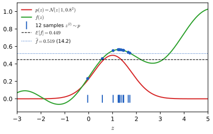
Result 14.1 (Monte Carlo error) pp. 430–431, (14.2)–(14.4); Exercises 14.1, 14.2
- If the \(\bz^{(l)}\) are drawn from \(p\), then \(\E[\widehat f]=\E[f]\); if they are also independent and \(\var[f]<\infty\), then \(\var[\widehat f]=\var[f]/L\) (14.4), and by the central limit theorem \(\widehat f\pm1.96\sqrt{\var[f]/L}\) is an approximate 95% interval.
- If instead they form a stationary sequence with autocorrelations \(\rho_k\)
\({}=\mathrm{corr}(f(\bz^{(l)}),f(\bz^{(l+k)}))\), the mean is unchanged and \[ \var[\widehat f]=\frac{\var[f]}{L}\Big[1+2\sum_{k=1}^{L-1}\Big(1-\frac kL\Big)\rho_k\Big]\approx\frac{\var[f]}{L}\,\tau_{\rm int},\qquad\tau_{\rm int}=1+2\sum_{k\ge1}\rho_k , \] so \(L\) correlated draws are worth \(L_{\rm eff}=L/\tau_{\rm int}\) independent ones (the "effective sample size" of p. 431). For \(\rho_k=\rho^k\), \(\tau_{\rm int}=(1+\rho)/(1-\rho)\).
Proof (short; the full argument is Result 11.2 of the companion course)
(1) Linearity: \(\E[\widehat f]\)
(2) \(\var[\widehat f]\)
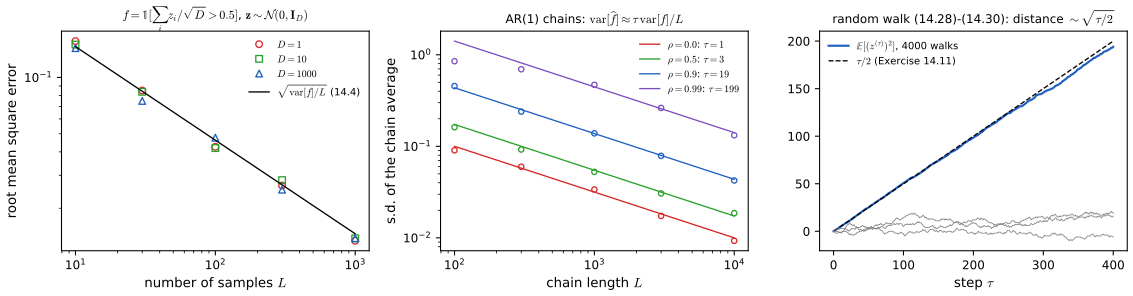
A direct computation confirms both statements: 40 000 repetitions of \(L=20\) draws give \(L\var[\widehat f]=1.376\) against \(\var[f]=1.370\), and an AR(1) chain with \(\rho=0.9\) gives \(L\var[\widehat f]=18.7\) against \(\tau_{\rm int}=19\).
Filling the gap 14.1: what "independent of the dimensionality" does and does not mean p. 431
The book notes that the \(1/L\) decrease does not depend on the dimension of \(\bz\), and that the error can still be large when \(f\) is large where \(p\) is small. Both statements can be made quantitative.
Derivation
The rate is dimension-free, the constant is not. (14.4) involves \(\bz\) only through the scalar \(\var[f]\). A grid with \(n\) points per axis would need \(n^D\) evaluations; Monte Carlo reaches standard error \(\varepsilon\) with \(L=\var[f]/\varepsilon^2\) draws in any dimension. But \(\var[f]\) itself may grow with \(D\): for \(f(\bz)=\|\bz\|^2\), \(\bz\sim\N(\bzero,\bI_D)\), \(\var[f]=2D\). In Figure 14.S1(a) \(f=\Ind[\sum_iz_i/\sqrt D>0.5]\) has the same variance \(P(1-P)\), \(P=1-\Phi(0.5)\), for every \(D\), and the measured error is indeed the same for \(D=1\), 10 and 1000.
Rare events. Let \(f=\Ind[\bz\in A]\) with \(P=p(A)\) small. Then \(\var[f]=P(1-P)\) and the relative error is \[\frac{\sqrt{\var[\widehat f]}}{P}=\sqrt{\frac{1-P}{LP}},\] so \(L\) must be much larger than \(1/P\) before \(\widehat f\) is even of the right order: this is the precise form of "the expectation may be dominated by regions of small probability". Importance sampling (Section 14.1.5) attacks exactly this case by drawing from a proposal that puts more mass on \(A\).
Correlation. Markov chain samples (Section 14.2) are correlated, and Result 14.1(2) shows the cost: for an AR(1) sequence with \(\rho=0.99\), \(\tau_{\rm int}=199\), so 10 000 steps are worth 50 independent draws (Figure 14.S1(b)). Keeping only every \(M\)th sample ("thinning", p. 441) makes the kept ones nearly independent but never lowers the variance of the average of a given run. ∎
Beyond the book: gradients of expectations
In deep learning the expectation (14.1) is often a training objective whose distribution depends on the parameters, \(J(\btheta)\)
Filling the gap 14.2: the score-function and reparameterisation estimators, their variances, and when each fails supplement to Section 14.1.1; the book's (19.17)
Let \(q(\bz\given\btheta)\) be differentiable in \(\btheta\). We compare the two unbiased estimators of \(\nabla_\btheta\E_q[f]\) and compute their variances for a Gaussian.
Derivation
Score-function (REINFORCE, likelihood-ratio) estimator (Williams, 1992). If differentiation under the integral is allowed (for example, if \(|f(\bz)\,\nabla_\btheta q(\bz\given\btheta)|\) is bounded near \(\btheta\) by an integrable function of \(\bz\), by dominated convergence), then, using \(\nabla q=q\nabla\ln q\),
\[ \nabla_\btheta\E_q[f]=\int f(\bz)\nabla_\btheta q(\bz\given\btheta)\,\d\bz=\E_q\big[f(\bz)\,\nabla_\btheta\ln q(\bz\given\btheta)\big]\simeq\frac1L\sum_lf(\bz^{(l)})\nabla_\btheta\ln q(\bz^{(l)}\given\btheta). \]
Only values of \(f\) are needed: \(f\) may be discontinuous or a black box. Taking \(f\equiv1\) gives \(\E_q[\nabla_\btheta\ln q]\)
Reparameterisation estimator. Suppose \(\bz=g(\beps,\btheta)\) with \(\beps\sim r(\beps)\) not depending on \(\btheta\), e.g. \(z=\mu+\sigma\epsilon\), \(\epsilon\sim\N(0,1)\) (the book's (19.17)). Then \(\E_q[f]=\E_r[f(g(\beps,\btheta))]\), and if \(f\) is differentiable with a dominating bound,
\[ \nabla_\btheta\E_q[f]=\E_r\big[(\nabla_\btheta g)^\T\nabla_\bz f(g(\beps,\btheta))\big]. \]
For the Gaussian: \(\partial_\mu\) gives \(f'(z)\), \(\partial_\sigma\) gives \(f'(z)\epsilon\). The score function for the same family is \(f(z)\epsilon/\sigma\) (for \(\mu\)) and \(f(z)(\epsilon^2-1)/\sigma\) (for \(\sigma\)), since \(\ln\N(z\given\mu,\sigma^2)\)
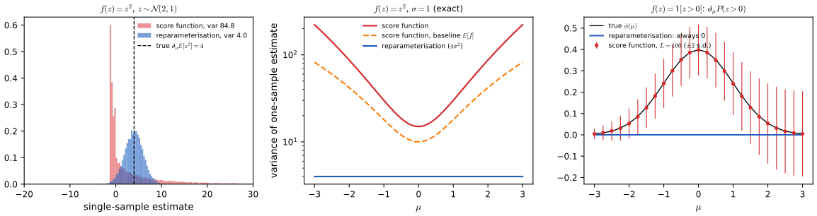
Exact variances for \(f(z)=z^2\), \(\theta=\mu\). The true gradient is \(\partial_\mu(\mu^2+\sigma^2)=2\mu\). Reparameterisation: \(\var[2(\mu+\sigma\epsilon)]=4\sigma^2\), whatever \(\mu\). Score function: with \(\E\epsilon^2=1\), \(\E\epsilon^4=3\), \(\E\epsilon^6=15\) and odd moments zero,
\[ \E\Big[\frac{(\mu+\sigma\epsilon)^4\epsilon^2}{\sigma^2}\Big]=\frac{\mu^4+6\mu^2\sigma^2\cdot3+\sigma^4\cdot15}{\sigma^2},\qquad\var=\frac{\mu^4+18\mu^2\sigma^2+15\sigma^4}{\sigma^2}-4\mu^2 , \]
which is 87 at \(\mu=2\), \(\sigma=1\) against 4, and grows like \(\mu^4\). With the baseline \(b=\E[f]=\mu^2+\sigma^2\), \((f-b)\epsilon/\sigma\)
When reparameterisation is wrong. For \(f=\Ind[z>a]\), \(f'=0\) wherever it exists, so the reparameterisation estimate is exactly \(0\), while \(\partial_\mu P(z>a)\)
When reparameterisation loses. For \(f=\sin(az)\), \(\var[f'(z)]\)
Link to this chapter. (14.55) is the score-function identity applied to the unnormalised density: \(\nabla_\bw\ln Z(\bw)\)
14.1.2 Standard distributions
See also the companion course, Section 11.1.1 (standard distributions), and Section 2.4 of these notes (transformation of densities).
pp. 431–433 If \(z\) is uniform on \((0,1)\) and \(y=g(z)\), the change-of-variables formula gives
\[ p(y)=p(z)\left|\frac{\d z}{\d y}\right| \tag{14.5} \]with \(p(z)=1\). Choosing \(g\) so that \(z\) equals the cumulative distribution function of the target,
\[ z=\int_{-\infty}^yp(\widehat y)\,\d\widehat y\equiv h(y), \tag{14.6} \]gives \(y=h^{-1}(z)\) (Figure 14.2). For the exponential distribution
\[ p(y)=\lambda\exp(-\lambda y),\qquad y\ge0, \tag{14.7} \]\(h(y)=1-e^{-\lambda y}\) and \(y=-\lambda^{-1}\ln(1-z)\); for the Cauchy distribution
\[ p(y)=\frac1\pi\frac1{1+y^2} \tag{14.8} \]\(h(y)=\frac12+\frac1\pi\arctan y\) and \(y=\tan\{\pi(z-\frac12)\}\) (Exercise 14.4). In several dimensions the Jacobian determinant replaces the derivative,
\[ p(y_1,\dots,y_M)=p(z_1,\dots,z_M)\left|\frac{\partial(z_1,\dots,z_M)}{\partial(y_1,\dots,y_M)}\right|. \tag{14.9} \]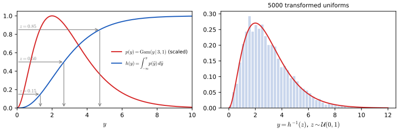
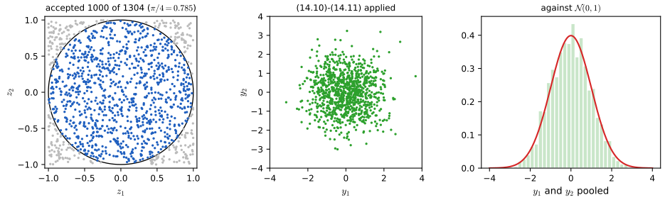
Box–Muller. Draw \(z_1,z_2\) uniform on \((-1,1)\), keep the pair only if \(r^2=z_1^2+z_2^2\le1\) (Figure 14.3), and set
\[ y_1=z_1\Big(\frac{-2\ln r^2}{r^2}\Big)^{1/2}, \tag{14.10} \] \[ y_2=z_2\Big(\frac{-2\ln r^2}{r^2}\Big)^{1/2}. \tag{14.11} \]Then
\[ p(y_1,y_2)=p(z_1,z_2)\left|\frac{\partial(z_1,z_2)}{\partial(y_1,y_2)}\right|=\Big[\frac1{\sqrt{2\pi}}e^{-y_1^2/2}\Big]\Big[\frac1{\sqrt{2\pi}}e^{-y_2^2/2}\Big], \tag{14.12} \]two independent standard Gaussians. A general Gaussian follows by \(y\mapsto\mu+\sigma y\), and a multivariate one by \(\by=\bmu+\bL\bz\) with \(\Sig=\bL\bL^\T\) (Cholesky).
Result 14.2 (the transformation method, Box–Muller, Cholesky) pp. 431–433; Exercises 14.3–14.6
- If \(h\) is continuous and strictly increasing on the support of \(p\) and \(z\sim\Unif(0,1)\), then \(y=h^{-1}(z)\) has density \(p\).
- The polar Box–Muller map sends the uniform distribution on the unit disc (density \(1/\pi\)) to \(\N(\bzero,\bI_2)\); a pair is accepted with probability \(\pi/4\).
- If \(\bz\sim\N(\bzero,\bI)\) and \(\Sig=\bL\bL^\T\), then \(\bmu+\bL\bz\sim\N(\bmu,\Sig)\).
Proof (short; full versions in Results 11.3, 11.4 and 11.5 of the companion course)
(1) \(P(y\le a)\)
(2) In polar coordinates \(z=r(\cos\theta,\sin\theta)\), the map keeps \(\theta\) and sends \(r\) to \(R=\sqrt{-2\ln r^2}\), so \(r^2=e^{-R^2/2}\). Area elements are \(r\,\d r\,\d\theta\) and \(R\,\d R\,\d\theta\); from \(R^2=-4\ln r\), \(R\,\d R=-2\,\d r/r\), so \(\big|\partial(y_1,y_2)/\partial(z_1,z_2)\big|\)
(3) An affine image of a Gaussian vector is Gaussian, with mean \(\bmu\) and covariance \(\bL\,\E[\bz\bz^\T]\bL^\T\)
The transformation method needs \(h\) and its inverse in closed form, which is rare, so we turn to rejection and importance sampling. They are limited to low dimensions but serve as building blocks.
14.1.3 Rejection sampling
See also the companion course, Section 11.1.2 (rejection sampling), and the rejection-sampling preset of its demo.
pp. 433–435 Suppose we can evaluate
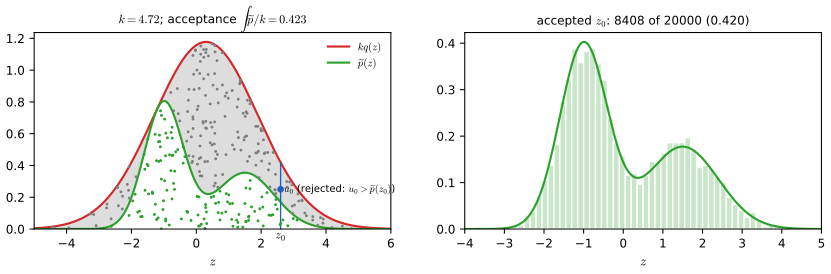
\[ p(\bz)=\frac1{Z_p}\pt(\bz) \tag{14.13} \]only up to the constant \(Z_p\). Choose a proposal \(q\) that is easy to sample and a constant \(k\) with \(kq(\bz)\ge\pt(\bz)\) everywhere (the comparison function). Draw \(z_0\sim q\), then \(u_0\) uniform on \([0,kq(z_0)]\); the pair is uniform under the graph of \(kq\). Reject it if \(u_0>\pt(z_0)\) (the grey region of Figure 14.4), otherwise keep \(z_0\). (Erratum. The book says "\(u_0\) is retained"; it is \(z_0\) that is kept.) The acceptance probability is
\[ p(\text{accept})=\int\{\pt(\bz)/kq(\bz)\}\,q(\bz)\,\d\bz=\frac1k\int\pt(\bz)\,\d\bz. \tag{14.14} \]Result 14.3 (rejection sampling is exact) pp. 433–434, (14.14); Exercise 14.7
If \(q(\bz)>0\) wherever \(\pt(\bz)>0\) and \(kq\ge\pt\), the accepted values have density \(p\), and the acceptance probability is \(Z_p/k\). Any such \(k\) works; the smallest one maximises the acceptance rate.
Proof (short; full version in Result 11.7)
Given \(z_0=\bz\), acceptance has probability \(P(u_0\le\pt(\bz))=\pt(\bz)/kq(\bz)\). By the product rule the joint density of "\(\bz\) drawn and accepted" is \(q(\bz)\pt(\bz)/kq(\bz)=\pt(\bz)/k\); by the sum rule \(P(\text{accept})=\int\pt/k=Z_p/k\), which is (14.14); and by Bayes' theorem the density of accepted values is \((\pt/k)/(Z_p/k)=p\). ∎
Sampling a gamma density. For
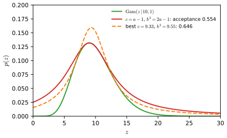
\[ \Gam(z\given a,b)=\frac{b^az^{a-1}\exp(-bz)}{\Gamma(a)} \tag{14.15} \]with \(a>1\), a bell-shaped Cauchy comparison function is natural. Transforming a uniform variable \(y\) on \((-\pi/2,\pi/2)\) by \(z=b\tan y+c\) gives Cauchy values, and the comparison function is
\[ kq(z)=\frac{k}{1+(z-c)^2/b^2}. \tag{14.16} \](The book writes the left side as \(q(z)\); as printed it is the comparison function \(kq\), since the normalised Cauchy density is \(1/\{\pi b(1+(z-c)^2/b^2)\}\).)
Filling the gap 14.3: the Cauchy envelope of the gamma density, and the claim that \(c=a-1\), \(b^2=2a-1\) minimise the rejection rate pp. 434–435, (14.16), Figure 14.5; Exercise 14.8
The book states that the minimum reject rate is obtained with \(c=a-1\) and \(b^2=2a-1\). That choice is valid and reasonable, but it is not the minimum.
Derivation
Acceptance rate of a Cauchy envelope. For given \((c,b)\) the smallest valid constant is \(k(c,b)\)
The book's choice is valid. With \(c=a-1\) (the mode) and \(k\) equal to the density at the mode, the envelope lies above the gamma for every \(a>1\) exactly when \(b^2\ge2a-1\); the sign argument is written out in the companion course, Filling the gap 11.4. So \(b^2=2a-1\) is the narrowest envelope among those that touch the gamma at its mode.
It is not optimal. Nothing forces the envelope to touch at the mode. Maximising \(1/\{k(c,b)\pi b\}\) over both \(c\) and \(b\) numerically (with \(k\) recomputed for each candidate) gives, for \(a=10\), \(c=9.33\), \(b^2=9.55\) and acceptance 0.646, against 0.554 for the book's \(c=9\), \(b^2=19\): the rejection rate falls from 44.6% to 35.4%. The optimal envelope is narrower and taller and touches the gamma on both flanks instead of at the peak (Figure 14.5). Simulation confirms both rates (0.555 and 0.646 observed).
Exercise 14.8. As printed, \(z\) is uniform on \([0,1]\); then \(y=b\tan z+c\) lies in \([c,c+b\tan1]\) and is not Cauchy. With \(z\) uniform on \((-\pi/2,\pi/2)\) (or \(y=b\tan\{\pi(z-\frac12)\}+c\) for \(z\) on \((0,1)\)) the inverse map is \(z=\arctan\{(y-c)/b\}\) and \(|\d z/\d y|=b/\{b^2+(y-c)^2\}\), so by (14.5) \(p(y)=\frac1\pi\frac{b}{b^2+(y-c)^2}\), a Cauchy density with location \(c\) and scale \(b\). ∎
14.1.4 Adaptive rejection sampling
See also the companion course, Section 11.1.3, Result 11.8 and Algorithm 11.2.
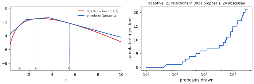
pp. 435–437 If \(\ln p\) is concave, its tangent lines lie above it, so the piecewise-linear minimum of the tangents at a few abscissae is an upper bound on \(\ln p\) (Figure 14.6). The envelope is then piecewise exponential,
\[ q(z)=k_i\lambda_i\exp\{-\lambda_i(z-z_{i-1})\},\qquad z_{i-1}<z\le z_i, \tag{14.17} \]where here \(z_{i-1},z_i\) are the breakpoints where successive tangents meet. Sample from the envelope, apply the rejection test, and add every rejected point to the abscissae: the envelope tightens and the rejection rate falls (Gilks and Wild, 1992). Without log-concavity a Metropolis–Hastings step can follow each rejection step (Gilks, Best and Tan, 1995).
Result 14.4 (the tangent envelope and how to sample it) pp. 435–436, (14.17); Exercises 14.9, 14.10
Let \(h_j=\ln p(\zeta_j)\) and \(g_j=(\ln p)'(\zeta_j)\) at abscissae \(\zeta_1<\dots<\zeta_n\). Successive tangents meet at \(e_j\)
Proof (short; details in Filling the gap 11.5)
A concave function lies below each of its tangents, so the envelope (their minimum) is above \(\ln p\); on each interval the lowest tangent is the one at the abscissa inside it, and two neighbouring tangents are equal at \(e_j\), which is the formula above. The masses are integrals of exponentials. On piece \(j\) the normalised density is \(\lambda e^{-\lambda(z-e_{j-1})}/(1-e^{-\lambda\Delta})\), \(\Delta=e_j-e_{j-1}\), whose CDF \((1-e^{-\lambda(z-e_{j-1})})/(1-e^{-\lambda\Delta})\) set equal to \(u\) gives the inversion formula (for \(\lambda=0\) the piece is uniform; unbounded end pieces need \(\lambda>0\) on the right and \(\lambda<0\) on the left). A direct computation confirms the masses against numerical integrals and the sampler by a Kolmogorov–Smirnov test. ∎
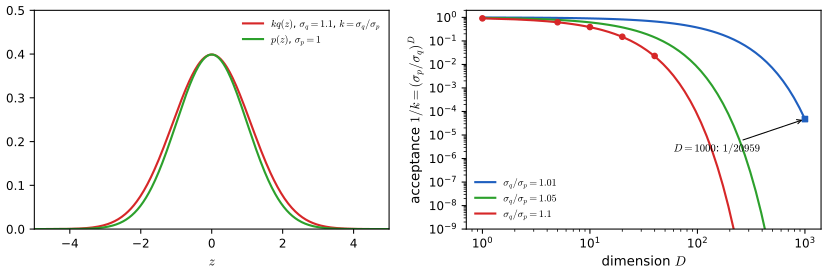
Rejection sampling in high dimensions. pp. 436–437 Sample \(\N(\bzero,\sigma_p^2\bI_D)\) with the proposal \(\N(\bzero,\sigma_q^2\bI_D)\), \(\sigma_q\ge\sigma_p\). Both densities peak at the origin, so the smallest \(k\) is the ratio of the peaks, \(k=(\sigma_q/\sigma_p)^D\), and the acceptance rate is \(1/k\).
Result 14.5 (acceptance falls exponentially with dimension) pp. 436–437, Figure 14.7
For the Gaussians above, \(p(\text{accept})\)
Proof (short; see also Result 11.9)
\(p(\bz)/q(\bz)\)
14.1.5 Importance sampling
See also the companion course, Section 11.1.4, Results 11.10–11.12, and the importance-sampling preset of its demo.
pp. 437–439 A uniform grid,
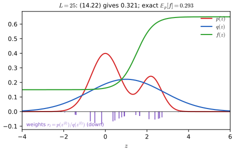
\[ \E[f]\simeq\sum_{l=1}^Lp(\bz^{(l)})f(\bz^{(l)}), \tag{14.18} \]needs exponentially many points in high dimension and wastes most of them where \(pf\) is negligible. Importance sampling draws from a proposal \(q\) instead (Figure 14.8):
\[ \E[f]=\int f(\bz)p(\bz)\,\d\bz=\int f(\bz)\frac{p(\bz)}{q(\bz)}q(\bz)\,\d\bz\simeq\frac1L\sum_{l=1}^L\frac{p(\bz^{(l)})}{q(\bz^{(l)})}f(\bz^{(l)}). \tag{14.19} \]The importance weights \(r_l=p(\bz^{(l)})/q(\bz^{(l)})\) correct for sampling from the wrong distribution, and no sample is discarded. If \(p=\pt/Z_p\) and \(q=\qt/Z_q\) are known only up to constants,
\[ \E[f]=\frac{Z_q}{Z_p}\int f(\bz)\frac{\pt(\bz)}{\qt(\bz)}q(\bz)\,\d\bz\simeq\frac{Z_q}{Z_p}\frac1L\sum_{l=1}^L\widetilde r_lf(\bz^{(l)}), \tag{14.20} \]with \(\widetilde r_l\)
so that
\[ \E[f]\simeq\sum_{l=1}^Lw_lf(\bz^{(l)}), \tag{14.22} \] \[ w_l=\frac{\widetilde r_l}{\sum_m\widetilde r_m}=\frac{\pt(\bz^{(l)})/q(\bz^{(l)})}{\sum_m\pt(\bz^{(m)})/q(\bz^{(m)})}. \tag{14.23} \]Result 14.6 (importance sampling: bias, consistency, effective sample size) pp. 437–439, (14.19)–(14.23)
- If \(q>0\) wherever \(pf\ne0\), (14.19) and (14.21) are unbiased; the variance of (14.19) is \(\frac1L\big(\int f^2p^2/q\,\d\bz-\E[f]^2\big)\), which is infinite if \(q\) has lighter tails than \(p|f|\).
- The self-normalised estimate (14.22) is a ratio of two unbiased averages: it is biased for finite \(L\), with bias \(O(1/L)\), but consistent, and its asymptotic variance is \(\frac1L\E_p[(p/q)(f-\E_p f)^2]\).
- A common summary of weight degeneracy is \(L_{\rm eff}=1/\sum_lw_l^2\), which is \(L\) for equal weights and 1 when a single weight dominates.
Proof (short; full version in Results 11.10–11.12 and Filling the gap 11.6)
(1) Each term has mean \(\int f\frac pqq=\E[f]\) and second moment \(\int f^2p^2/q\). (2) Write (14.22) as \(A_L/B_L\) with \(A_L\)
The book's warning on p. 439, that importance sampling can be badly wrong "with no diagnostic indication", is (1) at work: if \(q\) misses a region where \(pf\) is large, the sample weights look well behaved although the estimator's true variance is huge or infinite.
14.1.6 Sampling-importance-resampling
See also the companion course, Section 11.1.5 and Result 11.13; the SIR preset of its demo.
pp. 439–440 SIR avoids the constant \(k\) of rejection sampling: draw \(\bz^{(1)},\dots,\bz^{(L)}\) from \(q\), compute the weights (14.23), and draw \(L\) values from the discrete distribution on \(\{\bz^{(l)}\}\) with probabilities \(w_l\). In one dimension the distribution function of a resampled value is
\[ p(z\le a)=\sum_{l:z^{(l)}\le a}w_l=\frac{\sum_l\Ind(z^{(l)}\le a)\,\pt(z^{(l)})/q(z^{(l)})}{\sum_l\pt(z^{(l)})/q(z^{(l)})} , \tag{14.24} \]and as \(L\to\infty\) both sums divided by \(L\) converge to integrals against \(q\),
\[ p(z\le a)=\frac{\int\Ind(z\le a)\{\pt(z)/q(z)\}q(z)\,\d z}{\int\{\pt(z)/q(z)\}q(z)\,\d z}=\frac{\int\Ind(z\le a)\pt(z)\,\d z}{\int\pt(z)\,\d z}=\int\Ind(z\le a)p(z)\,\d z . \tag{14.25} \]Moments can be taken directly from the weighted draws,
\[ \E[f(\bz)]=\int f(\bz)p(\bz)\,\d\bz=\frac{\int f(\bz)[\pt(\bz)/q(\bz)]q(\bz)\,\d\bz}{\int[\pt(\bz)/q(\bz)]q(\bz)\,\d\bz}\simeq\sum_{l=1}^Lw_lf(\bz_l). \tag{14.26} \]Result 14.7 (what resampling does and does not change) pp. 439–440, (14.24)–(14.26)
(1) The limit (14.25) holds almost surely for every \(a\) if \(q>0\) where \(p>0\) and \(\E_q[\pt/q]<\infty\). (2) For finite \(L\), conditionally on the first-stage draws, the average of \(f\) over the resampled values has mean \(\sum_lw_lf(\bz^{(l)})\), the self-normalised estimate (14.22); resampling therefore adds variance and never removes bias. Its purpose is to produce unweighted samples, for example as input to a later stage.
Proof
(1) The law of large numbers applied to numerator and denominator of (14.24), each divided by \(L\), as written in (14.25). (2) Each resampled value equals \(\bz^{(l)}\) with probability \(w_l\), so its conditional expectation of \(f\) is \(\sum_lw_lf(\bz^{(l)})\). By the law of total variance, the variance of the resampled average is the variance of (14.22) plus the expected conditional (multinomial) variance, which is non-negative. See Result 11.13 of the companion course for (1) in more detail. ∎
14.2 Markov Chain Monte Carlo
See also the companion course, Section 11.2 (Markov chain Monte Carlo) and its Metropolis and Gibbs demo.
pp. 440–441 Rejection and importance sampling break down in high dimensions. Markov chain Monte Carlo (MCMC), which originated in physics (Metropolis and Ulam, 1949), scales much better: the proposal \(q(\bz\given\bz^{(\tau)})\) depends on the current state, so the samples \(\bz^{(1)},\bz^{(2)},\dots\) form a Markov chain, and an acceptance rule makes \(p\) the chain's long-run distribution. Only \(\pt\) is needed.
14.2.1 The Metropolis algorithm
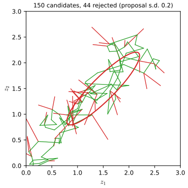
pp. 441–442 With a symmetric proposal, \(q(\bz_A\given\bz_B)\)
A move uphill in \(p\) is always accepted. If the candidate is rejected the chain stays put and the current state is recorded again; dropping the repeats would bias the samples.
Algorithm 14.1 (Metropolis sampling) p. 442
- Start from \(\bz^{(0)}\).
- For \(\tau=1,\dots,T\): draw \(\bz^\star\sim q(\bz\given\bz^{(\tau-1)})\) and \(u\sim\Unif(0,1)\); if \(\pt(\bz^\star)/\pt(\bz^{(\tau-1)})>u\) set \(\bz^{(\tau)}=\bz^\star\), otherwise \(\bz^{(\tau)}=\bz^{(\tau-1)}\).
- Return \(\bz^{(1)},\dots,\bz^{(T)}\) (the book returns only \(\bz^{(T)}\)).
(The comment "Iterative message-passing" in the book's listing is a leftover from another algorithm, and its "Output: \(\bz\sim\pt(\bz)\)" means a draw from the normalised \(p\).)
Random walks are slow. p. 442 On the integers, let the chain stay put with probability \(\frac12\) and move one step left or right with probability \(\frac14\) each,
\[ p(z^{(\tau+1)}=z^{(\tau)})=0.5, \tag{14.28} \] \[ p(z^{(\tau+1)}=z^{(\tau)}+1)=0.25, \tag{14.29} \] \[ p(z^{(\tau+1)}=z^{(\tau)}-1)=0.25. \tag{14.30} \]From \(z^{(0)}=0\), \(\E[z^{(\tau)}]=0\) and \(\E[(z^{(\tau)})^2]=\tau/2\) (Exercise 14.11; Figure 14.S1(c)): after \(\tau\) steps the walk has typically travelled only \(\sqrt{\tau/2}\). Avoiding this random-walk behaviour is a central aim in designing MCMC methods.
14.2.2 Markov chains
See also the companion course, Section 11.2.1, Definition 11.1 and Results 11.16–11.18.
Definition 14.1 (Markov chain, invariance, detailed balance, ergodicity) pp. 442–444, (14.31)–(14.34)
A first-order Markov chain satisfies
\[ p(\bz^{(m+1)}\given\bz^{(1)},\dots,\bz^{(m)})=p(\bz^{(m+1)}\given\bz^{(m)}), \tag{14.31} \]and is specified by \(p(\bz^{(0)})\) and transition probabilities \(T_m(\bz^{(m)},\bz^{(m+1)})\equiv p(\bz^{(m+1)}\given\bz^{(m)})\); it is homogeneous if \(T_m=T\) for all \(m\). Marginals propagate by
\[ p(\bz^{(m+1)})=\int p(\bz^{(m+1)}\given\bz^{(m)})\,p(\bz^{(m)})\,\d\bz^{(m)}. \tag{14.32} \]A distribution \(p^\star\) is invariant (stationary) if
\[ p^\star(\bz)=\int T(\bz',\bz)\,p^\star(\bz')\,\d\bz', \tag{14.33} \]and \(T\) satisfies detailed balance with respect to \(p^\star\) (is reversible) if
\[ p^\star(\bz)T(\bz,\bz')=p^\star(\bz')T(\bz',\bz). \tag{14.34} \]The chain is ergodic if \(p(\bz^{(m)})\to p^\star\) from every starting distribution; \(p^\star\) is then the unique equilibrium distribution.
Result 14.8 (detailed balance, mixtures and compositions) pp. 444, (14.35)–(14.39)
- Detailed balance implies invariance: \[ \int p^\star(\bz')T(\bz',\bz)\,\d\bz'=\int p^\star(\bz)T(\bz,\bz')\,\d\bz' \tag{14.35} \] \[ =p^\star(\bz)\int p(\bz'\given\bz)\,\d\bz' \tag{14.36} \] \[ =p^\star(\bz). \tag{14.37} \]
- If \(p^\star\) is invariant for base transitions \(B_1,\dots,B_K\), it is invariant for the mixture \[ T(\bz',\bz)=\sum_{k=1}^K\alpha_kB_k(\bz',\bz) \tag{14.38} \] (\(\alpha_k\ge0\), \(\sum_k\alpha_k=1\)) and for the composition \[ T(\bz',\bz)=\sum_{\bz_1}\cdots\sum_{\bz_{K-1}}B_1(\bz',\bz_1)\cdots B_{K-1}(\bz_{K-2},\bz_{K-1})B_K(\bz_{K-1},\bz). \tag{14.39} \]
- If every \(B_k\) is reversible, so is the mixture and so is the palindromic composition \(B_1\cdots B_KB_K\cdots B_1\); the plain composition generally is not.
Erratum. The book's (14.39) sums over \(\bz_1,\dots,\bz_{n-1}\); the index should be \(K-1\), as above.
Proof (short; full version in Result 11.18)
(1) is (14.35)–(14.37): apply (14.34) inside the integral, then use that \(T(\bz,\cdot)\) is a probability distribution. On a finite space write \(\mathbf D=\diag(p^\star)\); invariance is \(p^\star B=p^\star\) and reversibility is \(\mathbf DB=B^\T\mathbf D\). (2) \(p^\star\sum_k\alpha_kB_k\)
Filling the gap 14.4: when does a chain converge to its invariant distribution? p. 444
The book says a homogeneous chain is ergodic "subject only to weak restrictions" (citing Neal, 1993). On a finite state space the restrictions are exactly two.
Derivation
Finite state space. If \(T\) is irreducible (every state can reach every other with positive probability in some number of steps) and aperiodic (the return times to a state have greatest common divisor 1), then the invariant distribution is unique and \(p(\bz^{(m)})\to p^\star\) geometrically fast from any start. This is the Perron–Frobenius theorem applied to the primitive matrix \(T\); a complete proof is Result 11.17 of the companion course. Both conditions are needed: the identity matrix (the book's example) is aperiodic but reducible and keeps any distribution; the swap \(\big(\begin{smallmatrix}0&1\\1&0\end{smallmatrix}\big)\) is irreducible but has period 2 and never converges from a point mass.
Metropolis–Hastings. If the proposal density is positive everywhere, every set of positive probability under \(p\) can be reached in one step, so the chain is irreducible; and since a proposal is rejected with positive probability somewhere, or the kernel has a density, the chain is aperiodic. This is why the book can say that positivity of \(q\) is sufficient (p. 441). General state spaces need the measure-theoretic versions of these notions (\(\varphi\)-irreducibility, Harris recurrence; Robert and Casella, 1999), but the intuition is the same.
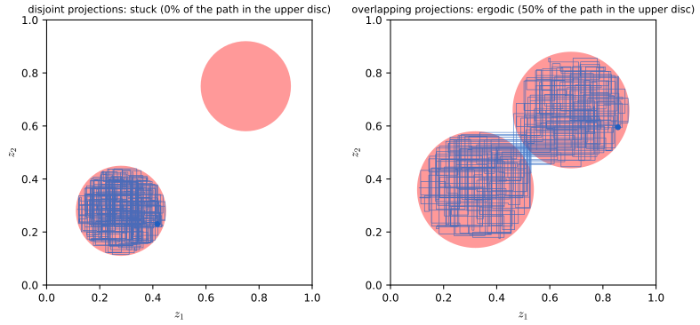
What fails in practice is not ergodicity but its speed: Figure 14.14 shows a Gibbs sampler that is not irreducible, and Figure 14.S3 a Langevin sampler that is ergodic but needs astronomically many steps to move mass between two wells. ∎
14.2.3 The Metropolis–Hastings algorithm
See also the companion course, Section 11.2.2 and Result 11.19.
pp. 445–446 For an asymmetric proposal \(q_k\) (\(k\) labels a family of proposals) the candidate is accepted with probability
\[ A_k(\bz^\star,\bz^{(\tau)})=\min\Big(1,\frac{\pt(\bz^\star)\,q_k(\bz^{(\tau)}\given\bz^\star)}{\pt(\bz^{(\tau)})\,q_k(\bz^\star\given\bz^{(\tau)})}\Big), \tag{14.40} \]which reduces to (14.27) for a symmetric proposal and again needs only \(\pt\).
Algorithm 14.2 (Metropolis–Hastings sampling) p. 446
- Start from \(\bz^{(0)}\); fix a rule \(k=M(\tau)\) choosing the proposal at step \(\tau\).
- For \(\tau=1,\dots,T\): draw \(\bz^\star\sim q_k(\bz\given\bz^{(\tau-1)})\) and \(u\sim\Unif(0,1)\); accept (\(\bz^{(\tau)}=\bz^\star\)) if \[ \frac{\pt(\bz^\star)\,q_k(\bz^{(\tau-1)}\given\bz^\star)}{\pt(\bz^{(\tau-1)})\,q_k(\bz^\star\given\bz^{(\tau-1)})}>u, \] otherwise repeat the old state.
(The book's listing drops the index \(k\) on \(q\) in the test.)
Result 14.9 (Metropolis–Hastings satisfies detailed balance) p. 445, (14.41)
For every proposal \(q_k\), the Metropolis–Hastings transition satisfies (14.34) with respect to \(p\), hence leaves \(p\) invariant:
\[ p(\bz)q_k(\bz'\given\bz)A_k(\bz',\bz)=\min\big(p(\bz)q_k(\bz'\given\bz),\,p(\bz')q_k(\bz\given\bz')\big)=p(\bz')q_k(\bz\given\bz')A_k(\bz,\bz'). \tag{14.41} \]Proof
For \(\bz'\ne\bz\) the transition density is \(T(\bz,\bz')\)
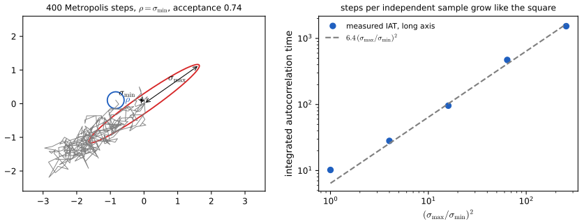
The scale of the proposal. pp. 445–446 With a Gaussian proposal of scale \(\rho\) on a target whose standard deviations range from \(\sigma_{\min}\) to \(\sigma_{\max}\) (Figure 14.10), \(\rho\) must be of order \(\sigma_{\min}\) to keep the rejection rate down, and the chain then explores the long direction by a random walk of step \(\sigma_{\min}\): reaching distance \(\sigma_{\max}\) takes about \((\sigma_{\max}/\sigma_{\min})^2\) steps. (For a multivariate Gaussian Neal (1993) refines this to \((\sigma_{\max}/\sigma_2)^2\), with \(\sigma_2\) the second-smallest standard deviation.)
Filling the gap 14.5: why about \((\sigma_{\max}/\sigma_{\min})^2\) steps per independent sample p. 445, Figure 14.10
Derivation
Along the long axis the chain moves by increments of size about \(\rho\approx\sigma_{\min}\), roughly independent and of mean near zero (the target is nearly flat on that scale). By the random-walk law of Exercise 14.11, \(\tau\) such steps cover a distance of order \(\sigma_{\min}\sqrt\tau\); to forget the starting point the chain must travel about \(\sigma_{\max}\), so \(\tau\approx(\sigma_{\max}/\sigma_{\min})^2\). The companion course gives the same argument in more detail (Filling the gap 11.9). Figure 14.10(b) measures it: with \(\rho=\sigma_{\min}\), the integrated autocorrelation time of the long-axis coordinate is close to \(6.4\,(\sigma_{\max}/\sigma_{\min})^2\) for ratios 2 to 16, and doubling the ratio multiplies it by 3.7 in simulation (theory: 4). ∎
14.2.4 Gibbs sampling
See also the companion course, Section 11.3 (Gibbs sampling), Results 11.20–11.22, and the Metropolis and Gibbs demo.
pp. 446–448 Gibbs sampling (Geman and Geman, 1984) replaces one variable \(z_i\) at a time by a draw from its conditional distribution \(p(z_i\given\bz_{\setminus i})\) given all the others, cycling through the variables or choosing them at random. With three variables, at step \(\tau\):
\[ z_1^{(\tau+1)}\sim p(z_1\given z_2^{(\tau)},z_3^{(\tau)}), \tag{14.42} \] \[ z_2^{(\tau+1)}\sim p(z_2\given z_1^{(\tau+1)},z_3^{(\tau)}), \tag{14.43} \] \[ z_3^{(\tau+1)}\sim p(z_3\given z_1^{(\tau+1)},z_2^{(\tau+1)}), \tag{14.44} \]each new value being used at once.
Algorithm 14.3 (Gibbs sampling) p. 448
- Initialise \(z_1,\dots,z_M\).
- For \(\tau=1,\dots,T\), for \(i=1,\dots,M\): draw \(z_i\sim p(z_i\given\{z_j\}_{j\ne i})\).
- Return the states (subsampled if nearly independent draws are wanted).
Result 14.10 (Gibbs sampling is Metropolis–Hastings that always accepts) pp. 447–448, (14.45); Exercise 14.12
- Each single-variable update leaves \(p\) invariant, and satisfies detailed balance.
- Viewed as Metropolis–Hastings with proposal \(q_k(\bz^\star\given\bz)\)
\({}=p(z_k^\star\given\bz_{\setminus k})\), \(\bz^\star_{\setminus k}\) \({}=\bz_{\setminus k}\), its acceptance ratio is \[ A(\bz^\star,\bz)=\frac{p(\bz^\star)q_k(\bz\given\bz^\star)}{p(\bz)q_k(\bz^\star\given\bz)}=\frac{p(z^\star_k\given\bz^\star_{\setminus k})p(\bz^\star_{\setminus k})p(z_k\given\bz^\star_{\setminus k})}{p(z_k\given\bz_{\setminus k})p(\bz_{\setminus k})p(z_k^\star\given\bz_{\setminus k})}=1. \tag{14.45} \] - A full systematic sweep is a composition (14.39): invariant, but in general not reversible; a random-scan sweep is a mixture (14.38) and is reversible.
- It is ergodic if, for example, no conditional is zero anywhere; if some are, ergodicity must be checked (Figure 14.14).
Proof (short; full version in Result 11.20)
(1) An update of \(z_k\) moves only to states \(\bz'\) with \(\bz'_{\setminus k}=\bz_{\setminus k}\), with kernel \(T(\bz,\bz')\)
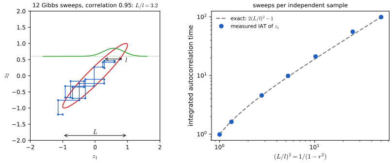
Gibbs on a correlated Gaussian. pp. 448–449 If the conditionals have width \(l\) and the marginals width \(L\) (Figure 14.11), each update moves about \(l\), and the book estimates \((L/l)^2\) steps per independent sample. For a bivariate Gaussian this can be computed exactly.
Result 14.11 (the exact cost of Gibbs sampling a bivariate Gaussian) p. 448, Figure 14.11
Let \((z_1,z_2)\) be Gaussian with unit variances and correlation \(r\), so \(L=1\) and the conditional standard deviation is \(l=\sqrt{1-r^2}\). Under systematic-scan Gibbs sampling, the sequence of \(z_1\) values (one per sweep) is an AR(1) process with coefficient \(r^2\), and its integrated autocorrelation time is
\[ \tau_{\rm int}=\frac{1+r^2}{1-r^2}=2\Big(\frac Ll\Big)^2-1 . \]Proof
The conditionals are \(z_2\given z_1\sim\N(rz_1,1-r^2)\) and \(z_1\given z_2\sim\N(rz_2,1-r^2)\). One sweep gives \(z_2'=rz_1+\sqrt{1-r^2}\,\xi_1\) and \(z_1'\)
Over-relaxation. p. 449 When the conditionals are Gaussian with mean \(\mu_i\) and variance \(\sigma_i^2\), Adler's (1981) over-relaxation replaces \(z_i\) by
\[ z_i'=\mu_i+\alpha_i(z_i-\mu_i)+\sigma_i(1-\alpha_i^2)^{1/2}\nu, \tag{14.46} \]with \(\nu\sim\N(0,1)\) and \(-1<\alpha_i<1\); \(\alpha=0\) is Gibbs sampling and \(\alpha<0\) pushes to the other side of the mean, which suppresses random-walk behaviour along strong correlations. Ordered over-relaxation (Neal, 1999) extends the idea beyond Gaussian conditionals.
Result 14.12 (over-relaxation leaves the conditional exactly invariant and is reversible) p. 449, (14.46); Exercise 14.14
If \(z_i\sim\N(\mu_i,\sigma_i^2)\) given the other variables, then so is \(z_i'\); the pair \((z_i,z_i')\) is bivariate Gaussian with correlation \(\alpha_i\) and the same marginals, hence exchangeable, so the update satisfies detailed balance.
Erratum. The book motivates the method with "the non-Gaussian distribution \(p(z,y)\propto\exp(-z^2y^2)\)", whose conditionals are Gaussian. That function cannot be normalised: \(\int e^{-z^2y^2}\d z=\sqrt\pi/|y|\), and \(\int\d y/|y|\) diverges at 0 and at \(\infty\) (numerically, the mass over \([10^{-K},10^K]\) growing linearly in \(K\)). A proper example is \(p(z,y)\propto\exp(-z^2y^2-z^2-y^2)\), whose conditionals are still Gaussian. Exercise 14.14 also writes "variance \(\sigma_i\)" for \(\sigma_i^2\).
Proof (see also Result 11.22)
\(z_i'\) is a linear combination of the independent Gaussians \(z_i\) and \(\nu\): \(\E[z_i']=\mu_i+\alpha_i\cdot0=\mu_i\), \(\var[z_i']\)
Markov blankets and blocking. pp. 449–450 In a directed graphical model the conditional of a node depends only on its Markov blanket (parents, children and co-parents; Figure 14.12, not reproduced since it is a diagram; see Result 8.10 and Filling the gap 11.10 of the companion course). Many such conditionals are log-concave, so adaptive rejection sampling can draw from them. Blocking Gibbs samplers update groups of variables jointly (Jensen, Kong and Kjærulff, 1995) to weaken the dependence between successive states.
14.2.5 Ancestral sampling
See also the companion course, Filling the gap 11.1 (logic sampling) and Filling the gap 11.7 (likelihood weighting).
pp. 450–451 For a directed graph with joint distribution
\[ p(\bz)=\prod_{i=1}^Mp(\bz_i\given\mathrm{pa}(i)), \tag{14.47} \]with the nodes numbered so that parents come first, one pass that draws each \(\bz_i\) from \(p(\bz_i\given\mathrm{pa}(i))\) with its parents already fixed gives an exact draw from the joint (ancestral sampling). With observed nodes (the evidence \(e\)), logic sampling (Henrion, 1988) discards a pass as soon as a sampled evidence node disagrees with its observed value; the survivors are exact posterior draws, but the acceptance probability \(p(e)\) shrinks rapidly with the amount of evidence. Likelihood weighting (Fung and Chang, 1990; Shachter and Peot, 1990) clamps the evidence nodes and samples the rest ancestrally, with weight
\[ r(\bz)=\prod_{\bz_i\notin e}\frac{p(\bz_i\given\mathrm{pa}(i))}{p(\bz_i\given\mathrm{pa}(i))}\prod_{\bz_i\in e}\frac{p(\bz_i\given\mathrm{pa}(i))}1=\prod_{\bz_i\in e}p(\bz_i\given\mathrm{pa}(i)). \tag{14.48} \]Result 14.13 (ancestral, logic and likelihood-weighted sampling) pp. 450–451, (14.47)–(14.48); Exercise 14.15
(1) Ancestral sampling draws exactly from (14.47). (2) Logic sampling is rejection sampling with proposal \(p(\bz)\) and acceptance probability \(p(e)\). (3) Likelihood weighting is importance sampling with proposal \(q(\bz_U)\)
Proof
(1) The probability of producing \(\bz\) is the product of the conditionals used, which is (14.47). (2) A pass survives iff its evidence nodes match \(e\), which happens with probability \(p(e)\); conditioned on surviving, the draw has density \(p(\bz)\Ind[\bz_e=e]/p(e)\)
14.3 Langevin Sampling
See also the companion course, Section 11.5 (hybrid Monte Carlo, the other sampler that uses gradients) and its slice sampling and HMC demo.
p. 451 Random-walk proposals ignore where the probability is. Just as gradients make training efficient, gradients of \(\ln p\) with respect to the data vector can steer a sampler uphill. Hamiltonian Monte Carlo does this with a Metropolis test (Duane et al., 1987); this section develops Langevin sampling, which in its basic form has no accept/reject step and is widely used in deep learning, notably for energy-based models.
14.3.1 Energy-based models
p. 452 A model \(p(\bx\given\bw)\) must integrate to one,
\[ \int p(\bx\given\bw)\,\d\bx=1, \tag{14.49} \](Erratum. The book prints \(\int p(\bx\given\bw)p(\bx)\,\d\bx=1\); the factor \(p(\bx)\) does not belong there.) Dropping this constraint gives much more freedom (LeCun et al., 2006).
Definition 14.2 (energy-based model, partition function) p. 452, (14.50)–(14.51)
Given any real-valued energy \(E(\bx,\bw)\), often a neural network with scalar output,
\[ p(\bx\given\bw)=\frac1{Z(\bw)}\exp\{-E(\bx,\bw)\}, \tag{14.50} \] \[ Z(\bw)=\int\exp\{-E(\bx,\bw)\}\,\d\bx , \tag{14.51} \]provided \(0<Z(\bw)<\infty\). Low energy means high probability. The name is used when \(Z\) cannot be computed.
Filling the gap 14.6: when (14.50) is a model, and which models are energy-based p. 452; Exercises 14.16, 14.17
Derivation
Normalisation (Exercise 14.16). \(\int p\,\d\bx\)
Every positive density is energy-based, with \(E=-\ln p\) and \(Z=1\); the energy is defined only up to an additive constant, which \(Z\) absorbs.
Log likelihood (Exercise 14.17). For i.i.d. data, \(\ln p(\mathcal D\given\bw)\)
p. 452 The partition function depends on \(\bw\), and so does the log likelihood of an i.i.d. data set \(\mathcal D=(\bx_1,\dots,\bx_N)\):
\[ \ln p(\mathcal D\given\bw)=-\sum_{n=1}^NE(\bx_n,\bw)-N\ln Z(\bw). \tag{14.52} \]14.3.2 Maximizing the likelihood
pp. 453–454 Training can avoid \(Z\) altogether (score matching, Chapter 20 of the book; Song and Kingma, 2021), or approximate the likelihood gradient by Monte Carlo, as here. For one data point,
\[ \nabla_\bw\ln p(\bx\given\bw)=-\nabla_\bw E(\bx,\bw)-\nabla_\bw\ln Z(\bw), \tag{14.53} \]and averaging over the data distribution \(p_{\mathcal D}\),
\[ \E_{\bx\sim p_{\mathcal D}}[\nabla_\bw\ln p(\bx\given\bw)]=-\E_{\bx\sim p_{\mathcal D}}[\nabla_\bw E(\bx,\bw)]-\nabla_\bw\ln Z(\bw). \tag{14.54} \]Differentiating (14.51),
\[ -\nabla_\bw\ln Z(\bw)=\int\{\nabla_\bw E(\bx,\bw)\}\,p(\bx\given\bw)\,\d\bx, \tag{14.55} \]an expectation under the model \(p_{\mathcal M}(\bx)=p(\bx\given\bw)\),
\[ \int\{\nabla_\bw E(\bx,\bw)\}\,p(\bx\given\bw)\,\d\bx=\E_{\bx\sim\mathcal M}[\nabla_\bw E(\bx,\bw)], \tag{14.56} \]so that
\[ \nabla_\bw\E_{\bx\sim p_{\mathcal D}}[\ln p(\bx\given\bw)]=-\E_{\bx\sim p_{\mathcal D}}[\nabla_\bw E(\bx,\bw)]+\E_{\bx\sim p_{\mathcal M}(\bx)}[\nabla_\bw E(\bx,\bw)]. \tag{14.57} \]Result 14.14 (the likelihood gradient of an energy-based model) pp. 453–454, (14.53)–(14.57); Exercise 14.18
- (14.55) and (14.57) hold whenever differentiation under the integral in (14.51) is allowed, for instance if \(\|\nabla_\bw E(\bx,\bw)\|e^{-E(\bx,\bw)}\) is bounded, for \(\bw\) in a neighbourhood, by an integrable function of \(\bx\).
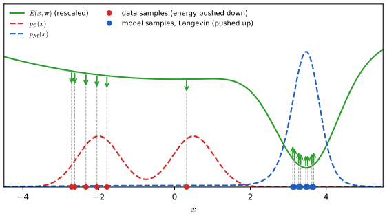
- Positive and negative phase. The first term of (14.57) lowers the energy (raises the density) at data points; the second raises it at samples from the model (Figure 14.13). Where \(p_{\mathcal M}>p_{\mathcal D}\) the net effect raises the energy, where \(p_{\mathcal M}<p_{\mathcal D}\) it lowers it.
- The second derivative is a covariance: \(\nabla_\bw\nabla_\bw^\T\ln Z\)
\({}=\cov_{\mathcal M}[\nabla_\bw E]-\E_{\mathcal M}[\nabla_\bw\nabla_\bw^\T E]\). For an energy linear in the parameters, \(E=E_0(\bx)+\bw^\T\bphi(\bx)\), \(\ln Z\) is convex, the average log likelihood is concave, and the gradient (14.57) vanishes exactly when \(\E_{p_{\mathcal D}}[\bphi]\) \({}=\E_{p_{\mathcal M}}[\bphi]\) (moment matching). - The gradient vanishes if \(p_{\mathcal M}=p_{\mathcal D}\) (as the book says), but not only then: a zero of (14.57) need not have \(p_{\mathcal M}=p_{\mathcal D}\) when the family cannot represent \(p_{\mathcal D}\).
Proof
(1) and Exercise 14.18. \(\nabla_\bw\ln Z\)
(2) A small step \(\Delta\bw=\epsilon\,g\) along the gradient changes the energy at \(\bx\) by \(\epsilon\nabla_\bw E(\bx)^\T g\). For the positive phase alone, \(g=-\E_{\mathcal D}[\nabla_\bw E]\), and averaged over the data the change is \(-\epsilon\|\E_{\mathcal D}[\nabla_\bw E]\|^2\le0\): energy goes down at the data. The negative phase does the opposite at model samples.
(3) Differentiate (14.55) once more: \(\nabla\nabla^\T\ln Z\)
(4) Take the demonstration's model (17 Gaussian bumps). Newton's method on the concave log likelihood reaches a point with \(\max_k|\partial/\partial w_k|\)
A direct computation confirms (14.55) and (14.57) against finite differences of the quadrature \(\ln Z\) (agreement to \(4\times10^{-10}\)) and the Hessian against the model covariance.
14.3.3 Langevin dynamics
pp. 454–455 The data term of (14.57) is an average over the training set,
\[ \E_{\bx\sim p_{\mathcal D}}[\nabla_\bw E(\bx,\bw)]\simeq\frac1N\sum_{n=1}^N\nabla_\bw E(\bx_n,\bw). \tag{14.58} \]The model term needs samples from \(p_{\mathcal M}\). Langevin sampling (Parisi, 1981; Welling and Teh, 2011) uses only the score, the gradient of the log density with respect to the data vector (not the parameters),
\[ \bs(\bx,\bw)=\nabla_\bx\ln p(\bx\given\bw), \tag{14.59} \]which for (14.50) is
\[ \bs(\bx,\bw)=-\nabla_\bx E(\bx,\bw): \tag{14.60} \]\(Z(\bw)\) has dropped out, because it does not depend on \(\bx\). Starting from \(\bx^{(0)}\) drawn from some initial distribution, iterate
\[ \bx^{(\tau+1)}=\bx^{(\tau)}+\eta\nabla_\bx\ln p(\bx^{(\tau)},\bw)+\sqrt{2\eta}\,\beps^{(\tau)},\qquad\tau\in1,\dots,T, \tag{14.61} \]with independent \(\beps^{(\tau)}\sim\N(\bzero,\bI)\) and step size \(\eta\): a gradient step uphill on \(\ln p\) plus Gaussian noise. The book states that as \(\eta\to0\) and \(T\to\infty\) the final value is a sample from \(p(\bx)\) (it writes \(\bz^{(T)}\) for \(\bx^{(T)}\)). Repeating gives samples \(\bx_1,\dots,\bx_M\) and
\[ \E_{\bx\sim p_{\mathcal M}(\bx)}[\nabla_\bw E(\bx,\bw)]\simeq\frac1M\sum_{m=1}^M\nabla_\bw E(\bx_m,\bw). \tag{14.62} \]Algorithm 14.4 (Langevin sampling) p. 456
- Input \(\bx^{(0)}\), the score of \(p(\bx,\bw)\), the step size \(\eta\) and the number of steps \(T\).
- For \(\tau=1,\dots,T\): draw \(\beps\sim\N(\bzero,\bI)\) and set \(\bx\leftarrow\bx+\eta\nabla_\bx\ln p(\bx,\bw)+\sqrt{2\eta}\,\beps\).
- Return \(\bx^{(T)}\).
Two names: in this book "score" means \(\nabla_\bx\ln p\), the gradient with respect to the data; the "score-function estimator" of Filling the gap 14.2 uses the statistician's score \(\nabla_\btheta\ln q\), the gradient with respect to parameters. With exact gradients (14.61) is often called the unadjusted Langevin algorithm; Welling and Teh's stochastic gradient Langevin dynamics is the same update with a mini-batch gradient (Filling the gap 14.8).
Why should (14.61) sample from \(p\)? The book says it "can be shown". Here is the argument in three steps: one step from \(p\) is correct to first order in \(\eta\); in the limit of small steps the dynamics has \(p\) as its exact stationary distribution; and for a Gaussian the leftover bias can be computed exactly.
Result 14.15 (one Langevin step leaves \(p\) invariant to first order) p. 455, (14.61)
Let \(p\) be smooth and positive with \(p\,\nabla\varphi\to0\) at infinity, and let \(\varphi\) be a smooth test function with bounded derivatives up to order four. If \(\bx\sim p\) and \(\bx'\)
with \(\Delta\) the Laplacian. Over the \(t/\eta\) steps needed to cover a fixed "time" \(t\), the per-step defects add up to \(O(\eta)\): the stationary distribution of (14.61) differs from \(p\) by \(O(\eta)\), and is exactly \(p\) only in the limit \(\eta\to0\).
Proof
Taylor expansion. Write \(\bx'=\bx+\Delta\) with \(\Delta=\eta\bs+\sqrt{2\eta}\,\beps\). Then \(\E_\beps[\Delta]=\eta\bs\), \(\E_\beps[\Delta\Delta^\T]\)
The first-order term has mean zero under \(p\). Since \(p\,\bs=p\nabla\ln p=\nabla p\),
\[ \int p\,(\bs\cdot\nabla\varphi+\Delta\varphi)\,\d\bx=\int(\nabla p\cdot\nabla\varphi+p\,\Delta\varphi)\,\d\bx=\int\nabla\cdot(p\nabla\varphi)\,\d\bx=0 \]
by the divergence theorem, the boundary term vanishing by assumption. So \(\E_p[\varphi(\bx')]\)
Accumulation. Each step started at \(p\) moves the expectation of every such \(\varphi\) by \(O(\eta^2)\); the chain needs about \(t_{\rm mix}/\eta\) steps to mix, during which the defects accumulate to \(O(\eta)\). Result 14.16 shows this is sharp for a Gaussian (bias \(\eta/2\) in the variance). Numerically, for the double-well density \(p\propto e^{-x^4/4+x^2/2}\) the one-step defect of \(\varphi=\cos1.3x+0.2x^2\) falls from \(1.08\times10^{-4}\) to \(2.75\times10^{-5}\) when \(\eta\) is halved from 0.01, a factor 3.9 (theory: 4). ∎
Filling the gap 14.7: the continuous-time limit, its exact stationary distribution, and convergence p. 455
The phrase "in the limits \(\eta\to0\) and \(T\to\infty\)" refers to a stochastic differential equation of which (14.61) is the Euler–Maruyama discretisation with time step \(\eta\).
Derivation
The Langevin diffusion. Let \(\d\bx_t\)
\(p\) is stationary. At \(\rho_t=p\), \(\ln(\rho_t/p)=0\) and the right side vanishes: there is no discretisation error in continuous time.
Convergence. Differentiate the KL divergence and integrate by parts: \[ \frac{\d}{\d t}\KL(\rho_t\,\|\,p)=\int\partial_t\rho_t\,\ln\frac{\rho_t}p\,\d\bx=-\int\rho_t\,\Big\|\nabla\ln\frac{\rho_t}{p}\Big\|^2\d\bx\le0, \] (the term \(\int\partial_t\rho_t\,\d\bx=0\) drops out), with equality only if \(\rho_t\propto p\). The right side is the relative Fisher information; if \(p\) satisfies a logarithmic Sobolev inequality with constant \(\lambda\) (true, for example, for \(\lambda\)-strongly log-concave \(p\)), it is at least \(2\lambda\KL\), and the divergence decays like \(e^{-2\lambda t}\). For multimodal \(p\) the constant can be tiny and convergence very slow (Filling the gap 14.9).
Changing the noise. With noise \(c\sqrt{2\eta}\,\beps\) instead of \(\sqrt{2\eta}\,\beps\) (the demo's slider \(c\)), the Fokker–Planck equation becomes \(\partial_t\rho\)
Result 14.16 (Langevin sampling of a Gaussian: exact bias, stability, mixing time) p. 455, (14.61)
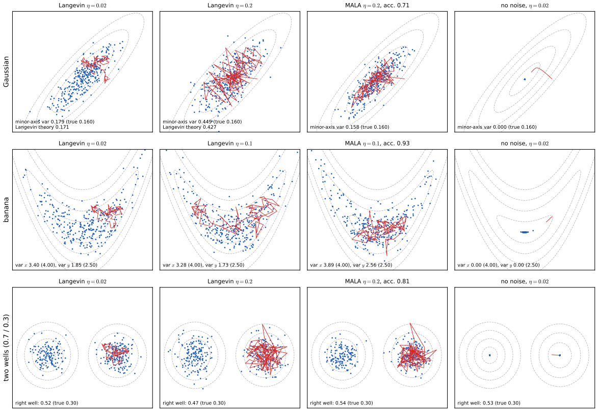
For \(p=\N(0,\sigma^2)\), (14.61) is \(x'\)
and the integrated autocorrelation time of \(x\) is \(2\sigma^2/\eta-1\). For \(\N(\bzero,\Sig)\) the same holds along each eigenvector of \(\Sig\) with its own \(\sigma_i^2\): stability needs \(\eta<2\sigma^2_{\min}\), and then the slowest direction has \(\tau_{\rm int}>\sigma^2_{\max}/\sigma^2_{\min}\), the condition number of \(\Sig\).
Proof
The score of \(\N(0,\sigma^2)\) is \(-x/\sigma^2\), so the update is AR(1) with coefficient \(a=1-\eta/\sigma^2\) and noise variance \(2\eta\). It is stable iff \(|a|<1\), i.e. \(0<\eta<2\sigma^2\). A stationary variance \(v\) must satisfy \(v=a^2v+2\eta\), so
\[ v=\frac{2\eta}{1-a^2}=\frac{2\eta}{2\eta/\sigma^2-\eta^2/\sigma^4}=\frac{\sigma^2}{1-\eta/(2\sigma^2)}, \]
and a Gaussian AR(1) process has a Gaussian stationary law. Its autocorrelations are \(a^k\), so Result 14.1(2) gives \(\tau_{\rm int}\)
This is the same trade-off as for gradient descent on a quadratic (Result 7.6): the steep direction limits the step, the shallow one sets the time. A simulation gives a stationary variance of 1.337 against \(4/3\) for \(\eta=0.5\), \(\sigma=1\), and \(\tau_{\rm int}=19.7\) against 19 for \(\eta=0.1\).
Result 14.17 (the Metropolis-adjusted Langevin algorithm, MALA) p. 451 ("an acceptance test"); Roberts and Tweedie (1996)
Use the Langevin move as a Metropolis–Hastings proposal, \(q(\bx'\given\bx)\)
The resulting chain leaves \(p\) exactly invariant for every \(\eta>0\) (no discretisation bias), and the acceptance rate tends to 1 as \(\eta\to0\).
Proof
The log of the proposal density is \(-\|\bx'-\bx-\eta\bs(\bx)\|^2/(4\eta)\) plus a constant that cancels in the ratio, which gives \(\ln A\). Detailed balance and invariance then follow from Result 14.9, whatever the proposal. As \(\eta\to0\), expanding the two squared norms shows that \(\ln A=O(\eta^{3/2})\) for typical \(\bx,\beps\) (the terms of order \(\eta^{1/2}\) and \(\eta\) cancel because the proposal is the discretisation of a \(p\)-reversible diffusion), so \(A\to1\). A direct computation confirms detailed balance numerically on the banana target and a variance of 0.996 (against 1) where unadjusted Langevin gives 1.337. ∎
langevin_run, the same code as the demo. Download: PDF · SVG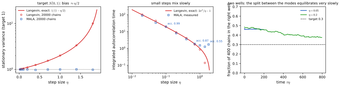
Filling the gap 14.8: stochastic gradient Langevin dynamics p. 455 (Welling and Teh, 2011)
Derivation
Welling and Teh (2011) sample a Bayesian posterior \(p(\btheta\given\mathcal D)\propto p(\btheta)\prod_{n=1}^Np(\bx_n\given\btheta)\) with the mini-batch estimate of its score, \(\widehat\bs\)
Why the mini-batch noise is harmless for small steps. Write \(\eta\widehat\bs\)
Filling the gap 14.9: "an independent sample in the limit": the problem of several modes p. 455
Derivation
The limit \(T\to\infty\) hides a time scale. For the two-well target of the demonstration (weights 0.7 and 0.3, means \(\pm2.5\), standard deviation 0.55), the log density at the midpoint is lower than at the modes by about \(2.5^2/(2\cdot0.55^2)\approx10\) nats. Transitions of a Langevin diffusion over such a barrier happen at a rate that decreases roughly like \(e^{-\Delta}\) with the barrier height \(\Delta\) (the Arrhenius–Kramers law of statistical physics, stated here without proof), so equilibrating the weights takes on the order of \(e^{10}\approx2\times10^4\) time units, millions of steps. Chains started from a broad distribution fall into the nearest well and stay; the fraction in each well reflects the starting distribution and the basins of attraction, not the target weights (Figure 14.S4(c); 53% instead of 30% after 3000 steps). MALA has the same problem: its acceptance step corrects the local shape, not the global weights. This is one motivation for the noise-perturbed scores of diffusion models (Chapter 20 of the book): at high noise the modes merge and can be traversed. ∎
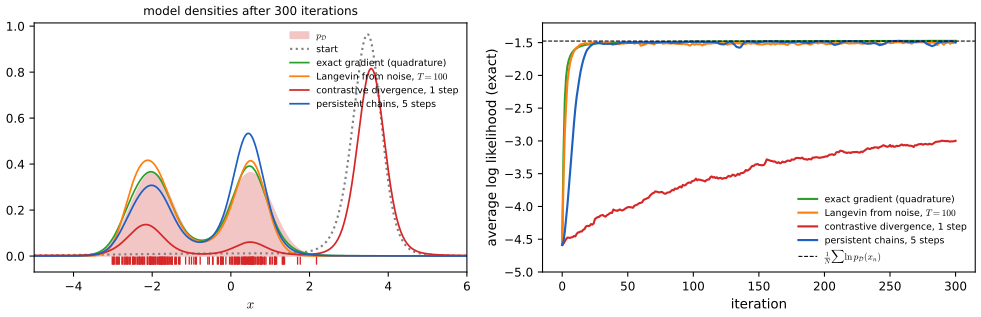
Contrastive divergence. p. 455 Long chains are expensive inside a training loop. Contrastive divergence (Hinton, 2002) starts each negative-phase chain at a training point and runs only a few steps, perhaps one. The samples are then biased towards the data, and the book remarks that this shapes the energy only near the data: useful for discrimination, less so for a generative model. This can be made precise.
Result 14.18 (what contrastive divergence optimises) p. 455
Let CD-\(k\) replace the model samples in (14.62) by \(\bx_n^{(k)}\), the result of \(k\) Langevin steps (14.61) from a data point \(\bx_n\). Its expected update direction is \(\frac1N\sum_n\big(\E[\nabla_\bw E(\bx_n^{(k)})]-\nabla_\bw E(\bx_n)\big)\). Then:
- for \(k=0\) the update is exactly zero; as \(k\to\infty\), if the chain is ergodic, it tends to the maximum-likelihood gradient (14.57);
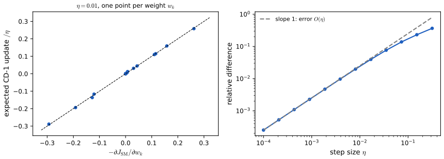
- for \(k=1\) and small \(\eta\), with \(\psi_j=\partial E/\partial w_j\) and the score \(s=-\partial E/\partial x\) (one dimension for simplicity), \[ \E[\psi_j(x_n^{(1)})]-\psi_j(x_n)=\eta\,\big(s\,\psi_j'+\psi_j''\big)(x_n)+O(\eta^2), \] and averaging over the data gives \(-\eta\,\partial J_{\rm SM}/\partial w_j+O(\eta^2)\), where \[ J_{\rm SM}(\bw)=\frac1N\sum_n\Big[\tfrac12s(x_n,\bw)^2+\partial_xs(x_n,\bw)\Big] \] is Hyvärinen's (2005) score-matching objective, equal up to a constant independent of \(\bw\) to \(\frac12\E_{p_{\mathcal D}}[(s-\partial_x\ln p_{\mathcal D})^2]\).
So CD-1 with Langevin steps is, to first order, gradient descent on score matching. Score matching compares only the slopes of \(\ln p\) at the data; it cannot see probability mass in regions where there are no data.
Proof
(1) For \(k=0\), \(\bx_n^{(0)}=\bx_n\) and the two terms cancel. For \(k\to\infty\), ergodicity gives \(\E[\nabla_\bw E(\bx_n^{(k)})]\to\E_{p_{\mathcal M}}[\nabla_\bw E]\) for every start (with the discretisation bias of Result 14.15 unless \(\eta\to0\) or a Metropolis correction is used), and the update tends to (14.57).
(2) The first display is Result 14.15 with \(\varphi=\psi_j\). For the second, differentiate \(J_{\rm SM}\): \(\partial s/\partial w_j\)
Consequence. In the demonstration the model starts with a deep well at \(x=3.5\), far from all data. The weights of the bumps there barely affect \(s\) or \(\partial_xs\) at the data, so score matching, and CD-1, leave the well in place: after 300 updates 75% of the model's mass is still at \(x>2\), while persistent chains (which wander into the well) and long chains from noise remove it (0.35% and 0.03%). A direct computation confirms the expansion: the relative difference between the expected CD-1 update divided by \(\eta\) and \(-\nabla J_{\rm SM}\) is \(2.5\times10^{-3}\) at \(\eta=10^{-3}\) and ten times smaller at \(\eta=10^{-4}\) (Figure 14.S6). ∎
Summary: errors and imprecisions found in the chapter (first printing)
- p. 434, rejection sampling: "otherwise \(u_0\) is retained" should read \(z_0\); \(u_0\) is only the auxiliary height.
- (14.16) and Exercise 14.8: the function written \(q(z)\) is the comparison function \(kq(z)\) (it is not normalised); with \(z\) uniform on \([0,1]\), \(y=b\tan z+c\) only takes values in \([c,c+b\tan1]\) and is not Cauchy; \(z\) must be uniform on \((-\pi/2,\pi/2)\) (checked: all values \(\ge c\), whereas a Cauchy puts half its mass below \(c\)).
- p. 435: \(c=a-1\), \(b^2=2a-1\) do not give "the minimum reject rate". For \(a=10\) the best Cauchy envelope has \(c=9.33\), \(b^2=9.55\) and accepts 64.6% against 55.4% (rejection 35.4% against 44.6%; both confirmed by simulation; Filling the gap 14.3).
- (14.39): the sums run over \(\bz_1,\dots,\bz_{K-1}\), not \(\bz_{n-1}\).
- Algorithms 14.1 and 14.2: the comment "Iterative message-passing" does not belong; Algorithm 14.2's test uses \(q\) where \(q_k\) is meant.
- p. 449: \(p(z,y)\propto\exp(-z^2y^2)\) is not a probability distribution (its integral diverges logarithmically; checked numerically); a proper example with Gaussian conditionals is \(\exp(-z^2y^2-z^2-y^2)\). Exercise 14.14: "variance \(\sigma_i\)" should be \(\sigma_i^2\).
- (14.49): \(\int p(\bx\given\bw)p(\bx)\,\d\bx=1\) should be \(\int p(\bx\given\bw)\,\d\bx=1\).
- Exercise 14.17: (14.52) is the log likelihood, not its gradient.
- p. 455: "the value of \(\bz^{(T)}\)" should be \(\bx^{(T)}\); and (14.61) with exact gradients is the unadjusted Langevin algorithm, while "stochastic gradient Langevin dynamics" (Welling and Teh, 2011) refers to the mini-batch version (Filling the gap 14.8).
- p. 454 (imprecision): the two terms of (14.57) balance when \(p_{\mathcal M}=p_{\mathcal D}\), but balance does not imply \(p_{\mathcal M}=p_{\mathcal D}\) (Result 14.14(4)).
Exercises
All 18 exercises of Chapter 14 (Bishop and Bishop, 2024, pp. 456–458), restated in my own words, with complete solutions (hidden). Stars give the book's difficulty. The official solutions manual stops at Chapter 10, so these solutions are my own; where a companion-course exercise is the same, it is linked.
Exercise 14.1 (★). Show that the Monte Carlo average (14.2) is an unbiased estimator of \(\E[f(\bz)]\).
Solution
By linearity of expectation and because each \(\bz^{(l)}\) has distribution \(p\), \(\E[\widehat f]\)
\({}=\frac1L\sum_{l=1}^L\E[f(\bz^{(l)})]\) \({}=\frac1L\cdot L\,\E[f]\) \({}=\E[f]\). Independence is not needed for this part. (Result 14.1; companion Exercise 11.1.) Exercise 14.2 (★). Show that (14.2) has the variance (14.4).
Solution
For independent draws, \(\var[\widehat f]\)
\({}=\frac1{L^2}\sum_l\var[f(\bz^{(l)})]\) \({}=\frac1L\var[f]\) \({}=\frac1L\E[(f-\E[f])^2]\), since the variance of a sum of independent terms is the sum of the variances. For correlated draws see Result 14.1(2). Checked by simulation: \(L\var[\widehat f]=1.376\) against 1.370. Exercise 14.3 (★). If \(z\sim\Unif(0,1)\) and \(y=h^{-1}(z)\) with \(h\) the indefinite integral (14.6) of \(p\), show that \(y\) has density \(p(y)\).
Solution
\(h\) is non-decreasing; assume it is continuous and strictly increasing where \(p>0\) (otherwise use the generalised inverse \(h^{-1}(z)=\inf\{y:h(y)\ge z\}\), for which \(h^{-1}(z)\le a\iff z\le h(a)\) still holds). Then \(P(y\le a)=P(z\le h(a))=h(a)\), so \(y\) has distribution function \(h\) and density \(h'=p\). Equivalently, by (14.5), \(p(y)=1\cdot|\d z/\d y|=h'(y)\). (Companion Exercise 11.2.)
Exercise 14.4 (★★). Find a transformation of a uniform \(z\) on \((0,1)\) that gives the Cauchy distribution (14.8).
Solution
\(h(y)\)
\({}=\int_{-\infty}^y\frac{\d t}{\pi(1+t^2)}\) \({}=\frac1\pi\big(\arctan y+\frac\pi2\big)\) \({}=\frac12+\frac1\pi\arctan y\). Solving \(z=h(y)\): \(y=\tan\{\pi(z-\frac12)\}\). Check: \(\d z/\d y=\frac1\pi\frac1{1+y^2}\). A simulation finds sample quartiles \(-0.98\), \(0.00\), \(0.99\) against \(-1,0,1\). (Companion Exercise 11.3.) Exercise 14.5 (★★). For \((z_1,z_2)\) uniform on the unit disc and \((y_1,y_2)\) given by (14.10)–(14.11), show that \((y_1,y_2)\) has the density (14.12).
Solution
See the proof of Result 14.2(2): in polar coordinates the map keeps the angle and sends radius \(r\) to \(R=\sqrt{-4\ln r}\); the Jacobian is \(|\partial(y_1,y_2)/\partial(z_1,z_2)|\)
\({}=2/r^2\), so \(p(\by)\) \({}=\frac1\pi\frac{r^2}2\) \({}=\frac1{2\pi}e^{-R^2/2}\), the product of two standard normal densities. A second route: \(\theta\) is uniform and \(r^2\sim\Unif(0,1)\) (since \(P(r^2\le t)=\pi t/\pi\)), so \(R^2=-2\ln r^2\) is exponential with mean 2, i.e. \(\chi^2_2\), which with an independent uniform angle is exactly the polar form of \(\N(\bzero,\bI_2)\). A direct computation verifies the Jacobian identity by finite differences. (Companion Exercise 11.4.) Exercise 14.6 (★★). If \(\bz\sim\N(\bzero,\bI_D)\) and \(\Sig=\bL\bL^\T\) is the Cholesky factorisation, show that \(\by=\bmu+\bL\bz\) is \(\N(\bmu,\Sig)\).
Solution
The characteristic function of \(\by\) is \(\E[e^{i\mathbf t^\T\by}]\)
\({}=e^{i\mathbf t^\T\bmu}\E[e^{i(\bL^\T\mathbf t)^\T\bz}]\) \({}=e^{i\mathbf t^\T\bmu-\frac12\mathbf t^\T\bL\bL^\T\mathbf t}\), that of \(\N(\bmu,\Sig)\). Directly: \(\E[\by]=\bmu\), \(\cov[\by]=\bL\E[\bz\bz^\T]\bL^\T=\Sig\). Only \(\bL\bL^\T=\Sig\) is used, not triangularity. (Companion Exercise 11.5.) Exercise 14.7 (★★). Show that rejection sampling accepts a proposal \(\bz\) with probability \(\pt(\bz)/kq(\bz)\), and, using the sum and product rules, that accepted values have density \(p(\bz)\).
Solution
Given \(\bz\), \(u_0\) is uniform on \([0,kq(\bz)]\), so \(P(\text{accept}\given\bz)\)
\({}=P(u_0\le\pt(\bz))\) \({}=\pt(\bz)/kq(\bz)\le1\). Product rule: the joint density of drawing \(\bz\) and accepting it is \(q(\bz)\pt(\bz)/kq(\bz)=\pt(\bz)/k\). Sum rule: \(P(\text{accept})=\int\pt/k=Z_p/k\). Conditional density: \((\pt/k)/(Z_p/k)=\pt/Z_p=p\). The exercise's requirement that \(k\) be the smallest valid constant is not needed: any \(k\) with \(kq\ge\pt\) works (Result 14.3; companion Exercise 11.6). Exercise 14.8 (★). Show that \(y=b\tan z+c\) has the Cauchy form (14.16) when \(z\) is uniform.
Solution
The uniform variable must range over \((-\pi/2,\pi/2)\), not over \([0,1]\) as printed (see Filling the gap 14.3). Then \(z=\arctan\{(y-c)/b\}\), \(\d z/\d y=\frac{1/b}{1+(y-c)^2/b^2}\), and with \(p(z)=1/\pi\), (14.5) gives \(p(y)\)
\({}=\frac1{\pi b}\frac1{1+(y-c)^2/b^2}\), which is (14.16) with \(k=1/(\pi b)\) for the normalised density; in the rejection sampler the comparison function is this times a constant. (Companion Exercise 11.7.) Exercise 14.9 (★★). Find the coefficients \(k_i\) of the piecewise exponential envelope (14.17) from continuity and normalisation.
Solution
Write the breakpoints as \(e_0<e_1<\dots<e_n\) (the book's \(z_{i-1},z_i\) in (14.17)) and the slopes \(\lambda_i=-g_i\), where \(g_i\) is the slope of the tangent used on piece \(i\). Continuity at \(e_i\): \(k_i\lambda_ie^{-\lambda_i(e_i-e_{i-1})}\)
\({}=k_{i+1}\lambda_{i+1}\), so \(k_{i+1}\) \({}=k_i\frac{\lambda_i}{\lambda_{i+1}}e^{-\lambda_i\Delta_i}\), \(\Delta_i=e_i-e_{i-1}\): all \(k_i\) are fixed by \(k_1\). Normalisation: \(\int_{e_{i-1}}^{e_i}k_i\lambda_ie^{-\lambda_i(z-e_{i-1})}\d z\) \({}=k_i(1-e^{-\lambda_i\Delta_i})\), so \(\sum_ik_i(1-e^{-\lambda_i\Delta_i})=1\) fixes \(k_1\). In terms of the tangents, \(k_i\lambda_i\) \({}=e^{h_i+g_i(e_{i-1}-\zeta_i)}/\sum_jM_j\) (Result 14.4), and the breakpoints are the tangent intersections. Interpretation: \(k_i\) is the mass the \(i\)th exponential would have if it were extended to infinity. A direct computation confirms the piece masses against numerical integration. (Companion Exercise 11.8.) Exercise 14.10 (★★). Using the method of Section 14.1.2, devise an algorithm for sampling the piecewise exponential distribution (14.17).
Solution
(i) Choose piece \(i\) with probability \(P_i=k_i(1-e^{-\lambda_i\Delta_i})\) (a discrete distribution: compare a uniform \(u_1\) with the cumulative sums). (ii) Within the piece the density is \(\lambda_ie^{-\lambda_i(z-e_{i-1})}/(1-e^{-\lambda_i\Delta_i})\), with distribution function \(F(z)\)
\({}=\frac{1-e^{-\lambda_i(z-e_{i-1})}}{1-e^{-\lambda_i\Delta_i}}\); setting \(F(z)=u_2\) gives \(z\) \({}=e_{i-1}-\lambda_i^{-1}\ln\{1-u_2(1-e^{-\lambda_i\Delta_i})\}\). For \(\lambda_i=0\) the piece is uniform; for an unbounded last piece (\(\Delta=\infty\), \(\lambda>0\)) the formula becomes \(z=e_{n-1}-\lambda^{-1}\ln(1-u_2)\), and similarly on the left with \(\lambda<0\). The two-stage draw has the right density because \(P(\text{piece }i)\times\) (density within the piece) \(=k_i\lambda_ie^{-\lambda_i(z-e_{i-1})}\). Implemented as ars_sample; a Kolmogorov–Smirnov test against the envelope passes. (Companion Exercise 11.9.)Exercise 14.11 (★). For the random walk (14.28)–(14.30), show that \(\E[(z^{(\tau)})^2]\)
\({}=\E[(z^{(\tau-1)})^2]+\frac12\), hence \(\E[(z^{(\tau)})^2]=\tau/2\). Solution
Write \(z^{(\tau)}=z^{(\tau-1)}+\xi_\tau\) with \(\xi_\tau\in\{0,+1,-1\}\) with probabilities \(\frac12,\frac14,\frac14\), independent of the past. Then \(\E[\xi_\tau]=0\), \(\E[\xi_\tau^2]=\frac12\), and \(\E[(z^{(\tau)})^2]\)
\({}=\E[(z^{(\tau-1)})^2]+2\E[z^{(\tau-1)}]\E[\xi_\tau]+\E[\xi_\tau^2]\) \({}=\E[(z^{(\tau-1)})^2]+\frac12\). With \(z^{(0)}=0\), induction gives \(\tau/2\). Verified exactly by propagating the distribution for 60 steps, and by 20 000 simulated walks (Figure 14.S1(c)). (Companion Exercise 11.10.) Exercise 14.12 (★★). Show that Gibbs sampling satisfies detailed balance (14.34).
Solution
Each single-variable update does: it only reaches states with \(\bz'_{\setminus k}=\bz_{\setminus k}\), and for those \[ p(\bz)T(\bz,\bz')=p(\bz_{\setminus k})\,p(z_k\given\bz_{\setminus k})\,p(z'_k\given\bz_{\setminus k}), \] symmetric in \(\bz\leftrightarrow\bz'\) (Result 14.10). A precise statement matters here: the systematic sweep \(B_1B_2\cdots B_M\) is not reversible in general (a two-binary-variable example has \(\max|\mathbf DT-(\mathbf DT)^\T|=0.053\)), although it keeps \(p\) invariant; the random-scan sampler and the palindromic sweep \(B_1\cdots B_MB_M\cdots B_1\) are reversible (Result 14.8). (Companion Exercise 11.11.)
Exercise 14.13 (★). For the distribution of Figure 14.14 (uniform on two regions), is standard Gibbs sampling ergodic, and does it sample correctly?
Solution
No. The two regions have disjoint projections on both axes. Starting in the lower region, the conditional of \(z_1\) given any reachable \(z_2\) is supported only on the lower region's chord, and likewise for \(z_2\); the upper region can never be reached, so the chain is reducible and its long-run distribution depends on the start (uniform on whichever region it started in). Averages then converge to conditional expectations given the starting region, not to expectations under \(p\). If the regions' projections overlap in at least one coordinate, a Gibbs move can jump between them and the sampler is ergodic. Both cases are simulated in Figure 14.14 (0% against 50% of the path in the upper region). Updating along other directions (for instance rotated coordinates, or a Metropolis move) would also restore ergodicity. (Companion Exercise 11.12.)
Exercise 14.14 (★). Show that the over-relaxation update (14.46), applied to \(z_i\) with mean \(\mu_i\) and variance \(\sigma_i^2\), with \(\nu\) of mean 0 and variance 1, gives \(z_i'\) with mean \(\mu_i\) and variance \(\sigma_i^2\).
Solution
\(\E[z_i']\)
\({}=\mu_i+\alpha_i(\E z_i-\mu_i)+\sigma_i\sqrt{1-\alpha_i^2}\,\E\nu\) \({}=\mu_i\). With \(\nu\) independent of \(z_i\), \(\var[z_i']\) \({}=\alpha_i^2\sigma_i^2+\sigma_i^2(1-\alpha_i^2)\) \({}=\sigma_i^2\). If \(z_i\) and \(\nu\) are Gaussian, \(z_i'\) is Gaussian too, so the conditional distribution itself (not just two moments) is preserved, and the update is reversible (Result 14.12). Checked with \(\alpha=-0.8\): mean 0.699, variance 1.686 (target 0.7, 1.69), correlation \(-0.800\). (The book writes "variance \(\sigma_i\)".) (Companion Exercise 11.14.) Exercise 14.15 (★). Show that the importance weights of likelihood-weighted sampling are (14.48).
Solution
The proposal samples each non-evidence node from its conditional given its (sampled or clamped) parents and sets evidence nodes to their observed values, so \(q(\bz)\)
\({}=\prod_{i\notin e}p(\bz_i\given\mathrm{pa}(i))\). The target, up to the constant \(p(e)\), is the joint with the evidence plugged in, \(\prod_{i\notin e}p(\bz_i\given\mathrm{pa}(i))\prod_{i\in e}p(\bz_i\given\mathrm{pa}(i))\). Their ratio is \(r(\bz)\) \({}=\prod_{i\in e}p(\bz_i\given\mathrm{pa}(i))\), (14.48); the unknown \(p(e)\) is handled by self-normalisation (14.22)–(14.23). (Result 14.13; companion Filling the gap 11.7.) Exercise 14.16 (★). Show that (14.50) is normalised when \(Z(\bw)\) is given by (14.51).
Solution
\(\int p(\bx\given\bw)\,\d\bx\)
\({}=\frac1{Z(\bw)}\int e^{-E(\bx,\bw)}\d\bx\) \({}=\frac{Z(\bw)}{Z(\bw)}\) \({}=1\), provided \(0<Z(\bw)<\infty\); see Filling the gap 14.6 for when that holds. A numerical experiment integrates the demonstration's model on its grid: \(|\int p-1|<10^{-12}\). Exercise 14.17 (★★). Using (14.50), show that the log likelihood of an energy-based model for i.i.d. data has the form (14.52).
Solution
By independence \(p(\mathcal D\given\bw)\)
\({}=\prod_np(\bx_n\given\bw)\), so \(\ln p(\mathcal D\given\bw)\) \({}=\sum_n\ln p(\bx_n\given\bw)\) \({}=\sum_n\{-E(\bx_n,\bw)-\ln Z(\bw)\}\) \({}=-\sum_nE(\bx_n,\bw)-N\ln Z(\bw)\). (The book's wording says "the gradient of the log likelihood"; (14.52) is the log likelihood itself, and its gradient is the subject of Exercise 14.18.) Exercise 14.18 (★★). Using (14.54)–(14.56), show that the gradient of the expected log likelihood is (14.57).
Solution
From (14.51), \(\nabla_\bw\ln Z\)
\({}=\frac1Z\int\nabla_\bw e^{-E}\d\bx\) \({}=-\int\nabla_\bw E\,\frac{e^{-E}}Z\,\d\bx\) \({}=-\E_{p_{\mathcal M}}[\nabla_\bw E]\), which is (14.55)–(14.56) (the interchange of derivative and integral needs the domination condition of Result 14.14(1)). Inserting into (14.54), whose last term does not depend on \(\bx\) and so passes through the expectation over \(p_{\mathcal D}\), gives (14.57). A direct computation confirms (14.55) and (14.57) against finite differences to \(4\times10^{-10}\).
Demonstrations
Three interactive pages, each linked above where its topic arises. They run in the browser and reproduce the Python code number for number (largest differences \(2\times10^{-16}\) for the Langevin chains, \(4\times10^{-15}\) for the trained weights, \(4\times10^{-11}\) for the gradient-estimator moments). The companion course's sampling basics demo already covers transformation, rejection, importance sampling and SIR, and its MCMC demo covers Metropolis and Gibbs, so the pages here concentrate on what this chapter adds.
- Langevin sampling on an energy landscape: hundreds of chains (14.61) on a correlated Gaussian, a banana and two wells; step size, noise scale, and the Metropolis correction (MALA). Presets: 1 small step, 2 large step and its bias, 3 MALA, 4 no noise, 5 two wells.
- Training an energy-based model: the positive and negative phases of (14.57) on a one-dimensional model with an exactly computable likelihood; exact, Langevin-from-noise, contrastive divergence and persistent chains. Presets: 1 exact, 2 from noise, 3 CD-1, 4 persistent, 5 CD-30.
- Score function versus reparameterisation: both estimators of a gradient of a Gaussian expectation, their histograms and exact variances, a baseline, and the cases where each fails. Presets: 1 smooth f, 2 baseline, 3 step function, 4 fast oscillation, 5 gradient in \(\sigma\).
References
- Bishop, C. M. and Bishop, H. (2024). Deep Learning: Foundations and Concepts. Springer, Cham. Chapter 14, pp. 429–458. doi:10.1007/978-3-031-45468-4. Book website: www.bishopbook.com.
- Bishop, C. M. (2006). Pattern Recognition and Machine Learning. Springer. Chapter 11.
- Adler, S. L. (1981). Over-relaxation method for the Monte Carlo evaluation of the partition function for multiquadratic actions. Physical Review D, 23(12), 2901–2904.
- Duane, S., Kennedy, A. D., Pendleton, B. J. and Roweth, D. (1987). Hybrid Monte Carlo. Physics Letters B, 195(2), 216–222.
- Fung, R. and Chang, K. C. (1990). Weighing and integrating evidence for stochastic simulation in Bayesian networks. In Uncertainty in Artificial Intelligence 5, 209–219.
- Geman, S. and Geman, D. (1984). Stochastic relaxation, Gibbs distributions, and the Bayesian restoration of images. IEEE Transactions on Pattern Analysis and Machine Intelligence, 6(6), 721–741.
- Gilks, W. R. and Wild, P. (1992). Adaptive rejection sampling for Gibbs sampling. Applied Statistics, 41(2), 337–348.
- Gilks, W. R., Best, N. G. and Tan, K. K. C. (1995). Adaptive rejection Metropolis sampling within Gibbs sampling. Applied Statistics, 44(4), 455–472.
- Gilks, W. R., Richardson, S. and Spiegelhalter, D. J. (eds) (1996). Markov Chain Monte Carlo in Practice. Chapman and Hall.
- Hastings, W. K. (1970). Monte Carlo sampling methods using Markov chains and their applications. Biometrika, 57(1), 97–109.
- Henrion, M. (1988). Propagation of uncertainty by logic sampling in Bayes' networks. In Uncertainty in Artificial Intelligence 2, 149–164.
- Hinton, G. E. (2002). Training products of experts by minimizing contrastive divergence. Neural Computation, 14(8), 1771–1800.
- Hyvärinen, A. (2005). Estimation of non-normalized statistical models by score matching. Journal of Machine Learning Research, 6, 695–709.
- Jensen, C. S., Kong, A. and Kjærulff, U. (1995). Blocking Gibbs sampling in very large probabilistic expert systems. International Journal of Human-Computer Studies, 42, 647–666.
- LeCun, Y., Chopra, S., Hadsell, R., Ranzato, M. and Huang, F. J. (2006). A tutorial on energy-based learning. In Predicting Structured Data, MIT Press.
- Metropolis, N. and Ulam, S. (1949). The Monte Carlo method. Journal of the American Statistical Association, 44(247), 335–341.
- Metropolis, N., Rosenbluth, A. W., Rosenbluth, M. N., Teller, A. H. and Teller, E. (1953). Equation of state calculations by fast computing machines. Journal of Chemical Physics, 21(6), 1087–1092.
- Neal, R. M. (1993). Probabilistic Inference Using Markov Chain Monte Carlo Methods. Technical report CRG-TR-93-1, University of Toronto.
- Neal, R. M. (1999). Suppressing random walks in Markov chain Monte Carlo using ordered overrelaxation. In Learning in Graphical Models, MIT Press, 205–228.
- Parisi, G. (1981). Correlation functions and computer simulations. Nuclear Physics B, 180, 378–384.
- Robert, C. P. and Casella, G. (1999). Monte Carlo Statistical Methods. Springer.
- Roberts, G. O. and Tweedie, R. L. (1996). Exponential convergence of Langevin distributions and their discrete approximations. Bernoulli, 2(4), 341–363.
- Shachter, R. D. and Peot, M. A. (1990). Simulation approaches to general probabilistic inference on belief networks. In Uncertainty in Artificial Intelligence 5, 221–231.
- Song, Y. and Kingma, D. P. (2021). How to train your energy-based models. arXiv:2101.03288.
- Welling, M. and Teh, Y. W. (2011). Bayesian learning via stochastic gradient Langevin dynamics. In Proceedings of the 28th International Conference on Machine Learning, 681–688.
- Williams, R. J. (1992). Simple statistical gradient-following algorithms for connectionist reinforcement learning. Machine Learning, 8, 229–256.
Every numerical statement in these notes comes from ch14_sampling.py.