Standard Distributions
Before neural networks can model distributions, we need the distributions they are built from. This chapter collects the standard ones: Bernoulli, binomial and multinomial for discrete data (Section 3.1); the multivariate Gaussian with its geometry, conditionals, marginals, the linear-Gaussian model, maximum likelihood and mixtures (3.2); the von Mises distribution for angles (3.3); the exponential family that contains most of them and explains why their maximum likelihood estimates match moments (3.4); and, at the other extreme, nonparametric estimators whose complexity grows with the data (3.5). Every later chapter uses these results: the Gaussian and categorical outputs of networks, the noise of diffusion models, the latent variables of VAEs and the mixtures of Chapter 15.
Ch. 1 Deep learning revolution Ch. 2 Probabilities Ch. 3 Standard distributions Ch. 4 Regression Ch. 5 Classification Ch. 6 Deep neural networks Ch. 7 Gradient descent Ch. 8 Backpropagation Ch. 9 Regularization Ch. 10 Convolutional networks Ch. 11 Structured distributions Ch. 12 Transformers Ch. 13 Graph neural networks Ch. 14 Sampling Ch. 15 Discrete latent variables Ch. 16 Continuous latent variables Ch. 17 GANs Ch. 18 Normalizing flows Ch. 19 Autoencoders Ch. 20 Diffusion models Appendices A to C
How to read these notes
They follow the book. Sections carry the book's numbers (3.1, 3.2.4, ...) and every displayed equation that appears in the book carries the book's equation number, e.g. (3.65). Equations without a number are steps the book skips.
Filling the gaps. Wherever the book says a result "is easily verified", "can be shown", or leaves it to an exercise, an orange Filling the gap box or a proof gives the complete argument. Proofs start hidden: open one with its bar, or use the button below the contents.
Figures and demonstrations. All sixteen figures of the chapter are recomputed from scratch by the Python code (including the three that the book draws as sketches). The ▶ Demo boxes open an interactive demonstration already set to the case under discussion. The main formulas, the figure numbers and the demos were also checked numerically.
Companion course: Bayesian and Probabilistic Machine Learning
Much of this chapter is also Chapter 2 of the companion course Bayesian and Probabilistic Machine Learning (which follows Bishop, 2006), where the classical results are proved in full and extended with their Bayesian treatment (conjugate priors, Student's t). Here the shared results get a statement, a short proof and a link; what this book presents differently (the linear-Gaussian model as the basis of later generative models, sequential estimation, moment matching, the deep-learning motivation) gets the full treatment. The overlapping sections are:
- Discrete variables: 2.1 Binary variables and 2.2 Multinomial variables.
- The Gaussian: 2.3 (geometry and moments), 2.3.1 conditional, 2.3.2 marginal, 2.3.3 Bayes' theorem, 2.3.4 maximum likelihood, 2.3.5 sequential estimation, 2.3.9 mixtures; mixtures and EM in depth in Chapter 9, Section 9.2.
- Periodic variables: 2.3.8. Exponential family: 2.4 and 2.4.1.
- Nonparametric methods: 2.5, 2.5.1 kernel estimators, 2.5.2 nearest neighbours, 2.5.3 consistency and the Cover–Hart bound.
- Tools: the completing-the-square, linear-Gaussian, Woodbury, Lagrange multiplier, matrix calculus and exponential family entries of its mathematical toolkit. Demos of the same ideas: density estimation, EM for Gaussian mixtures on Old Faithful, conjugate priors.
Main reference
C. M. Bishop and H. Bishop, Deep Learning: Foundations and Concepts, Springer (2024), Chapter 3, pages 65–110 (book website www.bishopbook.com). Section, equation, figure and exercise numbers below refer to this book.
The explanations, derivations, figures and code are my own; equations are cited by their numbers in the book.
The chapter at a glance
- 3.1 For binary and one-hot data the likelihood depends on the data only through counts, and maximum likelihood gives the observed fractions (Results 3.1–3.3).
- 3.2 The Gaussian is a product of independent 1-D Gaussians along the eigenvectors of \(\bSig\) (Result 3.4). Its conditionals and marginals are Gaussian: conditionals are simplest in the precision \(\bLam=\bSig^{-1}\), marginals in \(\bSig\) (Results 3.7, 3.9). The linear-Gaussian model \(p(\bx)p(\by|\bx)\) has a Gaussian marginal \(p(\by)\) and posterior \(p(\bx|\by)\) in closed form (Result 3.10). Maximum likelihood gives the sample mean and a biased sample covariance (Result 3.11); mixtures of Gaussians are flexible but have no closed-form fit.
- 3.3 Angles need their own distribution: the von Mises density is a 2-D Gaussian restricted to the unit circle, and its maximum likelihood estimates are the direction and length of the vector mean (Result 3.12).
- 3.4 All of these (except mixtures) are exponential families; the derivatives of \(-\ln g(\bet)\) are the moments of \(\bu(\bx)\), so maximum likelihood matches the model mean of \(\bu\) to its sample mean (Result 3.14).
- 3.5 Histograms, kernel density estimators and \(K\)-nearest neighbours trade bias for variance through one smoothing parameter; they store all the data, which motivates the parametric-but-flexible neural models of later chapters.
Notation. Vectors are bold lower case, matrices bold upper case; \(D\) is the dimension of \(\bx\), \(N\) the number of observations, \(\bSig\) a covariance and \(\bLam=\bSig^{-1}\) a precision matrix; \(|\bSig|\) is a determinant; \(\bx^\T\) a transpose. All logarithms are natural.
Prerequisites. Chapter 2 of the book (probability, the univariate Gaussian, entropy and KL divergence) and the matrix identities of its Appendix A.
pp. 65–66 Density estimation is the problem of choosing a distribution \(p(\bx)\) from a finite sample \(\bx_1,\dots,\bx_N\). It is ill-posed: any density that is positive at the data points could have produced them, so some restriction (a model class, a smoothness assumption) is unavoidable, and choosing it is a problem of model selection. The chapter first studies parametric families, fitted by maximum likelihood on independent and identically distributed (i.i.d.) data, and ends with nonparametric estimators whose effective number of parameters grows with \(N\). Deep networks sit in between: a large but fixed number of parameters, and very flexible distributions.
3.1 Discrete Variables
See also: companion course, Section 2.1 Binary variables and Section 2.2 Multinomial variables (with the beta and Dirichlet priors).
3.1.1 Bernoulli distribution
Definition 3.1 (Bernoulli distribution) pp. 66–67, (3.1)–(3.4)
A binary variable \(x\in\{0,1\}\) with \(p(x=1\given\mu)=\mu\) (3.1), \(0\le\mu\le1\), has the distribution
\[ \Bern(x\given\mu)=\mu^{x}(1-\mu)^{1-x}, \tag{3.2} \]with \(\E[x]=\mu\) (3.3) and \(\var[x]=\mu(1-\mu)\) (3.4).
Proof (normalisation and moments; Exercise 3.1)
The two values have probabilities \(\Bern(0\given\mu)=1-\mu\) and \(\Bern(1\given\mu)=\mu\), which sum to 1. Then \(\E[x]=0\cdot(1-\mu)+1\cdot\mu=\mu\). Because \(x^2=x\) for \(x\in\{0,1\}\), \(\E[x^2]=\mu\) and \(\var[x]=\E[x^2]-\E[x]^2=\mu-\mu^2\). ∎
Result 3.1 (maximum likelihood for the Bernoulli) p. 67, (3.5)–(3.8)
For i.i.d. observations \(\mathcal{D}=\{x_1,\dots,x_N\}\) the log likelihood
\[ \ln p(\mathcal{D}\given\mu)=\sum_{n=1}^N\{x_n\ln\mu+(1-x_n)\ln(1-\mu)\} \tag{3.6} \]depends on the data only through the sufficient statistic \(m=\sum_nx_n\), and it is maximised by the sample mean
\[ \mu_{\rm ML}=\frac1N\sum_{n=1}^Nx_n=\frac mN. \tag{3.7, 3.8} \]Proof (including the boundary cases the book does not mention)
Independence gives \(p(\mathcal{D}\given\mu)\)
3.1.2 Binomial distribution
Result 3.2 (the binomial distribution, its mean and variance) pp. 67–68, (3.9)–(3.12)
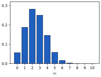
The number \(m\) of ones in \(N\) independent Bernoulli\((\mu)\) trials has the distribution
\[ \Bin(m\given N,\mu)=\binom Nm\mu^m(1-\mu)^{N-m},\qquad \binom Nm\equiv\frac{N!}{(N-m)!\,m!}, \tag{3.9, 3.10} \]for \(m=0,1,\dots,N\), with
\[ \E[m]=N\mu,\qquad \var[m]=N\mu(1-\mu). \tag{3.11, 3.12} \]Proof (counting, then two derivations of the moments)
The distribution. A particular sequence with \(m\) ones and \(N-m\) zeros has probability \(\mu^m(1-\mu)^{N-m}\) by independence, whatever the order. The number of such sequences is the number of ways to choose which \(m\) of the \(N\) (distinguishable) positions hold the ones, \(\binom Nm\). Adding the probabilities of these disjoint sequences gives (3.9). It is normalised by the binomial theorem: \(\sum_m\binom Nm\mu^m(1-\mu)^{N-m}\)
Moments by linearity. Write \(m=x_1+\dots+x_N\) with independent Bernoulli \(x_n\). Expectation is linear, so \(\E[m]=N\mu\); variances of independent variables add (the covariances vanish), so \(\var[m]=N\mu(1-\mu)\) by (3.4).
Moments by calculus (Exercise 3.4). Differentiate \(\sum_m\binom Nm\mu^m(1-\mu)^{N-m}=1\) with respect to \(\mu\): \(\sum_m\binom Nm\mu^m(1-\mu)^{N-m}\big(\tfrac m\mu\)
3.1.3 Multinomial distribution
pp. 68–70 A variable with \(K\) mutually exclusive states is coded one-hot (the 1-of-\(K\) scheme): \(\bx=(x_1,\dots,x_K)^\T\) with one \(x_k=1\) and the others 0, e.g. \(\bx=(0,0,1,0,0,0)^\T\) (3.13). This is the coding of class labels for every classification network in the book.
Result 3.3 (categorical and multinomial distributions; maximum likelihood) pp. 69–70, (3.14)–(3.24)
With \(\mu_k=p(x_k=1)\), \(\mu_k\ge0\), \(\sum_k\mu_k=1\), the distribution of one observation is
\[ p(\bx\given\bmu)=\prod_{k=1}^K\mu_k^{x_k}, \tag{3.14} \]which sums to 1 (3.15) and has \(\E[\bx\given\bmu]=\bmu\) (3.16). For \(N\) i.i.d. observations the likelihood is \(\prod_k\mu_k^{m_k}\) (3.17) with counts \(m_k=\sum_nx_{nk}\) (3.18), \(\sum_km_k=N\) (3.19), and the maximum likelihood estimate is
\[ \mu_k^{\rm ML}=\frac{m_k}N. \tag{3.22} \]The counts themselves have the multinomial distribution
\[ \Mult(m_1,\dots,m_K\given\bmu,N)=\binom{N}{m_1\,m_2\cdots m_K}\prod_{k=1}^K\mu_k^{m_k}, \tag{3.23} \] \[ \binom{N}{m_1\cdots m_K}=\frac{N!}{m_1!\cdots m_K!}. \tag{3.24} \]Proof (the Lagrangian of the book, and why its stationary point is the maximum)
(3.15)–(3.17). There are \(K\) possible \(\bx\), the unit vectors \(\mathbf{e}_k\), and \(p(\mathbf{e}_k\given\bmu)=\mu_k\), so the sum is \(\sum_k\mu_k=1\) and \(\E[\bx]=\sum_k\mu_k\mathbf{e}_k=\bmu\). The likelihood is \(\prod_n\prod_k\mu_k^{x_{nk}}\)
(3.20)–(3.22). Maximise \(\sum_km_k\ln\mu_k\) subject to \(\sum_k\mu_k=1\). The Lagrangian \(\sum_km_k\ln\mu_k+\lambda(\sum_k\mu_k-1)\) (3.20) has \(\partial/\partial\mu_k\)
Why this is the global maximum. The book stops at stationarity. The objective is concave on the simplex (each \(m_k\ln\mu_k\) is concave) and the constraint is linear, so any stationary point of the Lagrangian in the interior is a global maximum. A shorter argument avoids calculus altogether: with \(\hat\mu_k=m_k/N\),
\[ \frac1N\Big(\sum_km_k\ln\hat\mu_k-\sum_km_k\ln\mu_k\Big)=\sum_k\hat\mu_k\ln\frac{\hat\mu_k}{\mu_k}=\KL(\hat\bmu\,\|\,\bmu)\ge0, \]with equality only when \(\bmu=\hat\bmu\) (Gibbs' inequality). This also covers counts \(m_k=0\), where the Lagrangian derivative is not defined: those terms are absent and the KL argument still gives \(\mu_k=0\).
(3.23)–(3.24). Every sequence of \(N\) outcomes with counts \((m_1,\dots,m_K)\) has probability \(\prod_k\mu_k^{m_k}\), and the number of such sequences is the number of ways of splitting \(N\) labelled positions into groups of sizes \(m_1,\dots,m_K\): choose the \(m_1\) positions of state 1 in \(\binom N{m_1}\) ways, then the \(m_2\) of state 2 among the rest, and so on; the product telescopes to \(N!/(m_1!\cdots m_K!)\). The multinomial theorem \((\mu_1+\dots+\mu_K)^N\)
A two-state quantity can be coded either as a binary \(x\) (Bernoulli/binomial) or as a 1-of-2 vector (\(K=2\) in (3.14)); the two descriptions are equivalent. The companion course's toolkit entry on Lagrange multipliers gives the general theory used above.
3.2 The Multivariate Gaussian
See also: companion course, Section 2.3 The Gaussian distribution (geometry, moments, why sums become Gaussian, the linear algebra behind the Gaussian).
Definition 3.2 (univariate and multivariate Gaussian) p. 70, (3.25)–(3.26)
\[ \N(x\given\mu,\sigma^2)=\frac1{(2\pi\sigma^2)^{1/2}}\exp\Big\{-\frac1{2\sigma^2}(x-\mu)^2\Big\}, \tag{3.25} \] \[ \N(\bx\given\bmu,\bSig)=\frac1{(2\pi)^{D/2}}\frac1{|\bSig|^{1/2}}\exp\Big\{-\frac12(\bx-\bmu)^\T\bSig^{-1}(\bx-\bmu)\Big\}, \tag{3.26} \]with mean vector \(\bmu\in\R^D\) and a symmetric positive definite \(D\times D\) covariance matrix \(\bSig\) (the book writes \(\det\bSig\) and \(|\bSig|\) for the same determinant).
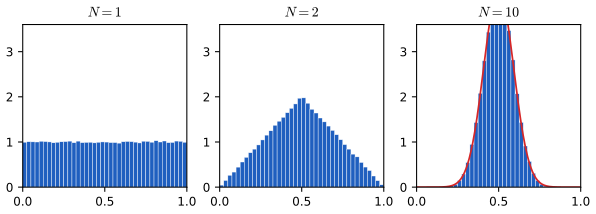
Why the Gaussian. Two of the book's motivations are stated without proof. (i) Among all densities with a given mean and covariance, the Gaussian has the largest entropy (Exercise 3.8, solved below). (ii) The central limit theorem: sums of many independent variables are approximately Gaussian, illustrated in Figure 3.2 with means of uniform variables.
Filling the gap 3.1: what the central limit theorem says, and the binomial limit p. 71
The book quotes the theorem informally ("subject to certain mild conditions"). Here are the statement and the two facts behind Figures 3.1 and 3.2.
Statement and proof sketch
Statement (Lindeberg–Lévy). Let \(x_1,x_2,\dots\) be i.i.d. with mean \(m\) and finite variance \(s^2>0\), and \(\bar x_N=\frac1N\sum_{n\le N}x_n\). Then \(\sqrt N(\bar x_N-m)/s\) converges in distribution to \(\N(0,1)\): for every \(t\), \(P\big(\sqrt N(\bar x_N-m)/s\)
Sketch. Let \(z_n=(x_n-m)/s\), so \(\E z_n=0\), \(\E z_n^2=1\), and let \(\varphi(t)=\E e^{itz_n}\) be the characteristic function. A second-order Taylor expansion, valid because the second moment is finite, gives \(\varphi(t)=1-t^2/2+o(t^2)\). The normalised sum \(S_N=N^{-1/2}\sum z_n\) has characteristic function \(\varphi(t/\sqrt N)^N\)
Figure 3.2. A uniform variable on \([0,1]\) has mean \(1/2\) and variance \(\int_0^1x^2\d x-\tfrac14=\tfrac1{12}\), so the mean of \(N\) of them is approximately \(\N(1/2,1/(12N))\), the curve drawn for \(N=10\). Convergence is fast here because the uniform density is symmetric (the leading correction, proportional to the skewness, vanishes).
Figure 3.1 and the binomial. \(m\) is a sum of \(N\) Bernoulli variables, so \((m-N\mu)/\sqrt{N\mu(1-\mu)}\) tends to \(\N(0,1)\) (the de Moivre–Laplace theorem): \(\Bin(m\given N,\mu)\)
3.2.1 Geometry of the Gaussian
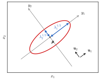
pp. 71–74 The density depends on \(\bx\) only through the squared Mahalanobis distance
\[ \Delta^2=(\bx-\bmu)^\T\bSig^{-1}(\bx-\bmu), \tag{3.27} \]which is the squared Euclidean distance when \(\bSig=\bI\). There is no loss in taking \(\bSig\) symmetric: an antisymmetric part \(\mathbf{K}\) (with \(\mathbf{K}^\T=-\mathbf{K}\)) of the matrix in a quadratic form contributes \(\ba^\T\mathbf{K}\ba\)
Result 3.4 (eigen-decomposition and the rotated coordinates) pp. 71–74, (3.28)–(3.40)
Let \(\bSig\) be real symmetric. Its eigenvalues are real and it has orthonormal eigenvectors, \(\bSig\bu_i=\lambda_i\bu_i\) (3.28), \(\bu_i^\T\bu_j=I_{ij}\) (3.29)–(3.30), and
\[ \bSig=\sum_{i=1}^D\lambda_i\bu_i\bu_i^\T,\qquad\bSig^{-1}=\sum_{i=1}^D\frac1{\lambda_i}\bu_i\bu_i^\T. \tag{3.31, 3.32} \]In the coordinates \(y_i=\bu_i^\T(\bx-\bmu)\) (3.34), i.e. \(\by=\bU(\bx-\bmu)\) with \(\bU\) the orthogonal matrix with rows \(\bu_i^\T\) (3.35),
\[ \Delta^2=\sum_{i=1}^D\frac{y_i^2}{\lambda_i}, \tag{3.33} \]and, if all \(\lambda_i>0\) (\(\bSig\) positive definite), the density factorises into independent one-dimensional Gaussians and is normalised:
\[ p(\by)=\prod_{j=1}^D\frac1{(2\pi\lambda_j)^{1/2}}\exp\Big\{-\frac{y_j^2}{2\lambda_j}\Big\},\qquad\int p(\by)\,\d\by=1. \tag{3.39, 3.40} \]The surfaces of constant density are ellipsoids centred at \(\bmu\) with axes along the \(\bu_i\) and semi-axis lengths \(\lambda_i^{1/2}\Delta\) (Figure 3.3).
Proof (spectral theorem, Jacobian and determinant; Exercises 3.12, 3.13)
Real eigenvalues. If \(\bSig\bu=\lambda\bu\) with \(\bu\ne\mathbf 0\) possibly complex, multiply on the left by the conjugate transpose \(\bu^{\dagger}\): \(\bu^\dagger\bSig\bu\)
Orthogonality for distinct eigenvalues. \(\lambda_j\bu_i^\T\bu_j\)
A full orthonormal basis, also for repeated eigenvalues. This is the step that needs care. Induct on \(D\). Take one unit eigenvector \(\bu_1\) (one exists: the eigenvalue equation \(|\bSig-\lambda\bI|=0\) has a root, real by the above). The subspace \(V=\{\bv:\bu_1^\T\bv=0\}\) is mapped into itself by \(\bSig\), since \(\bu_1^\T\bSig\bv\)
(3.31)–(3.32). Let \(\bU\) have rows \(\bu_i^\T\); orthonormality is \(\bU\bU^\T=\bI\), so \(\bU^\T=\bU^{-1}\) and \(\bU^\T\bU=\bI\) too. The eigen-equations read \(\bSig\bU^\T=\bU^\T\mathbf D\) with \(\mathbf D=\diag(\lambda_i)\), so \(\bSig=\bU^\T\mathbf D\bU\)
(3.33). Substituting (3.32): \(\Delta^2\)
(3.36)–(3.40). The inverse map is \(\bx=\bmu+\bU^\T\by\), so \(J_{ij}=\partial x_i/\partial y_j=U_{ji}\) (3.36) and \(|\bJ|^2=|\bU^\T||\bU|=|\bU^\T\bU|=1\) (3.37): the change of variables preserves volume. The determinant is the product of the eigenvalues, \(|\bSig|=|\bU^\T||\mathbf D||\bU|\)
Ellipsoids. \(\Delta^2=c^2\) reads \(\sum_iy_i^2/(c^2\lambda_i)=1\): an ellipsoid in the \(\by\)-coordinates with semi-axes \(c\lambda_i^{1/2}\) along the coordinate axes, which are the directions \(\bu_i\) in \(\bx\)-space. ∎
Positive definiteness. The normalisation needs every \(\lambda_i>0\). A symmetric matrix is positive definite, \(\ba^\T\bSig\ba>0\) for all \(\ba\ne\mathbf 0\), exactly when all its eigenvalues are positive: writing \(\ba=\sum_i\hat a_i\bu_i\) gives \(\ba^\T\bSig\ba\)
3.2.2 Moments
Result 3.5 (mean and covariance of the Gaussian) pp. 74–75, (3.41)–(3.48)
\[ \E[\bx]=\bmu,\qquad\E[\bx\bx^\T]=\bmu\bmu^\T+\bSig, \tag{3.42, 3.46} \] \[ \cov[\bx]=\E\big[(\bx-\E[\bx])(\bx-\E[\bx])^\T\big]=\bSig. \tag{3.47, 3.48} \]Proof (filling in the integral the book evaluates "by symmetry" in (3.45))
Substitute \(\bz=\bx-\bmu\) (3.41). The density of \(\bz\) is \(\N(\bz\given\mathbf0,\bSig)\), an even function of \(\bz\), so \(\E[\bz]=\mathbf0\) (the integrand \(\bz\,\N(\bz)\) is odd and integrable) and \(\E[\bx]=\bmu\). For the second moment, \(\E[\bx\bx^\T]\)
To compute \(\E[\bz\bz^\T]\) use \(\bz=\sum_jy_j\bu_j\) (3.44). By Result 3.4 the \(y_j\) are independent with \(y_j\sim\N(0,\lambda_j)\), and the change of variables has unit Jacobian, so
\[ \E[\bz\bz^\T]=\sum_{i,j}\bu_i\bu_j^\T\,\E[y_iy_j]=\sum_{i,j}\bu_i\bu_j^\T\,\lambda_i\delta_{ij}=\sum_i\lambda_i\bu_i\bu_i^\T=\bSig, \]because \(\E[y_iy_j]=\E[y_i]\E[y_j]=0\) for \(i\ne j\) (independence) and \(\E[y_i^2]=\lambda_i\) (the variance of a univariate Gaussian, the book's (2.53)), and the last step is (3.31). This is (3.45). Then \(\cov[\bx]\)
3.2.3 Limitations
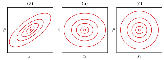
pp. 75–76 A symmetric \(D\times D\) matrix has \(D(D+1)/2\) free entries (the \(D\) diagonal entries and half of the \(D^2-D\) others, Exercise 3.15), so a full Gaussian has \(D(D+3)/2\) parameters, quadratic in \(D\), and inverting \(\bSig\) costs \(O(D^3)\). A diagonal covariance \(\diag(\sigma_i^2)\) has \(2D\) parameters and axis-aligned contours; an isotropic covariance \(\sigma^2\bI\) has \(D+1\) and spherical contours (Figure 3.4). The Gaussian is also unimodal. Latent variables fix both problems: discrete ones give mixtures (Section 3.2.9), continuous ones give models whose number of parameters is controlled separately from \(D\) (Chapter 16).
3.2.4 Conditional distribution
See also: companion course, Section 2.3.1 Conditional Gaussian distributions and the toolkit's completing the square.
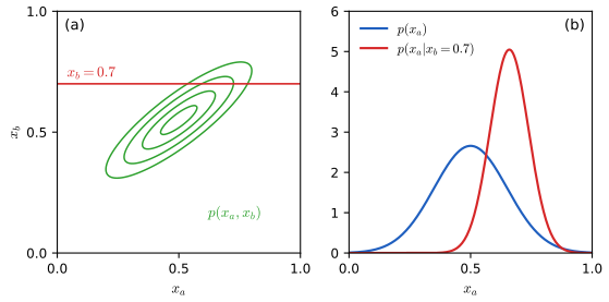
pp. 76–79 Partition \(\bx=(\bx_a,\bx_b)\) with \(\bx_a\in\R^M\), and partition \(\bmu\), \(\bSig\) and the precision matrix \(\bLam\equiv\bSig^{-1}\) (3.52) accordingly:
\[ \bx=\begin{pmatrix}\bx_a\\\bx_b\end{pmatrix},\quad\bmu=\begin{pmatrix}\bmu_a\\\bmu_b\end{pmatrix},\quad\bSig=\begin{pmatrix}\bSig_{aa}&\bSig_{ab}\\\bSig_{ba}&\bSig_{bb}\end{pmatrix},\quad\bLam=\begin{pmatrix}\bLam_{aa}&\bLam_{ab}\\\bLam_{ba}&\bLam_{bb}\end{pmatrix}. \tag{3.49–3.53} \]Symmetry gives \(\bSig_{ba}=\bSig_{ab}^\T\) and \(\bLam_{ba}=\bLam_{ab}^\T\) (the inverse of a symmetric matrix is symmetric: transpose \(\bM\bM^{-1}=\bI\), Exercise 3.16). Note that \(\bLam_{aa}\ne\bSig_{aa}^{-1}\) in general.
Result 3.6 (completing the square) p. 78, (3.55)
For symmetric \(\bSig\),
\[ -\frac12(\bx-\bmu)^\T\bSig^{-1}(\bx-\bmu)=-\frac12\bx^\T\bSig^{-1}\bx+\bx^\T\bSig^{-1}\bmu+\const. \tag{3.55} \]Hence if a density satisfies \(\ln p(\bx)\)
Proof (and why "reading off" is legitimate)
Expanding, \((\bx-\bmu)^\T\bSig^{-1}(\bx-\bmu)\)
Result 3.7 (the conditional of a joint Gaussian) pp. 77–79, (3.54)–(3.66), (3.80)–(3.81)
\(p(\bx_a\given\bx_b)\)
and, in covariance form,
\[ \bmu_{a|b}=\bmu_a+\bSig_{ab}\bSig_{bb}^{-1}(\bx_b-\bmu_b),\qquad\bSig_{a|b}=\bSig_{aa}-\bSig_{ab}\bSig_{bb}^{-1}\bSig_{ba}. \tag{3.65, 3.66} \]The mean is linear in \(\bx_b\) and the covariance does not depend on \(\bx_b\): a linear-Gaussian model.
Proof (completing the square in \(\bx_a\), then the partitioned inverse)
Precision form. By the product rule \(p(\bx_a\given\bx_b)\)
The second-order part in \(\bx_a\) is \(-\frac12\bx_a^\T\bLam_{aa}\bx_a\) (3.56). The first-order part collects \(\bx_a^\T\bLam_{aa}\bmu_a\) from the first term and \(-\frac12\bx_a^\T\bLam_{ab}(\bx_b-\bmu_b)\) from each of the middle two (the third equals the second because \(\bLam_{ba}^\T=\bLam_{ab}\)), giving \(\bx_a^\T\{\bLam_{aa}\bmu_a\)
Covariance form. The partitioned inverse (Result 3.8 below) applied to \(\bSig\) gives \(\bLam_{aa}\)
Erratum. The summary formula (3.80) prints \(p(\bx_a\given\bx_b)\)
Result 3.8 (inverse of a partitioned matrix; Schur complement) pp. 78–79, (3.60)–(3.64)
If \(\mathbf D\) and \(\bA-\mathbf B\mathbf D^{-1}\mathbf C\) are invertible, then
\[ \begin{pmatrix}\bA&\mathbf B\\\mathbf C&\mathbf D\end{pmatrix}^{-1}=\begin{pmatrix}\bM&-\bM\mathbf B\mathbf D^{-1}\\-\mathbf D^{-1}\mathbf C\bM&\mathbf D^{-1}+\mathbf D^{-1}\mathbf C\bM\mathbf B\mathbf D^{-1}\end{pmatrix}, \tag{3.60} \] \[ \bM=(\bA-\mathbf B\mathbf D^{-1}\mathbf C)^{-1}. \tag{3.61} \]\(\bM^{-1}\) is the Schur complement of \(\mathbf D\).
Proof (multiply out; Exercise 3.18)
Multiply the claimed inverse on the left by the block matrix. Top-left: \(\bA\bM-\mathbf B\mathbf D^{-1}\mathbf C\bM\)
Filling the gap 3.2: why every matrix inverted above is invertible, and positive definite pp. 77–81
The derivations invert \(\bLam_{aa}\), \(\bSig_{bb}\), \(\bLam_{bb}\) and Schur complements without comment. All of these are positive definite whenever \(\bSig\) is, so the conditional and marginal "Gaussians" are genuine, normalisable densities.
Derivation
Principal blocks. If \(\bSig\) is positive definite, so is \(\bSig_{bb}\): for \(\bv\ne\mathbf0\), \(\bv^\T\bSig_{bb}\bv\)
Schur complement. By (3.63), \(\bSig_{aa}-\bSig_{ab}\bSig_{bb}^{-1}\bSig_{ba}\)
is a congruence (the outer factors are transposes of each other and invertible), so the middle block-diagonal matrix is positive definite too, and so is its top-left block. The factorisation also gives \(|\bSig|=|\bSig_{a|b}|\,|\bSig_{bb}|\), the determinant version of \(p(\bx_a,\bx_b)\)
Conditioning reduces uncertainty. Because \(\bSig_{ab}\bSig_{bb}^{-1}\bSig_{ba}\) is positive semidefinite, \(\bSig_{a|b}\preceq\bSig_{aa}\): observing \(\bx_b\) never increases the covariance of \(\bx_a\), and it leaves it unchanged exactly when \(\bSig_{ab}=\mathbf0\), i.e. when \(\bx_a\) and \(\bx_b\) are uncorrelated (and, for a Gaussian, independent). ∎
3.2.5 Marginal distribution
See also: companion course, Section 2.3.2 Marginal Gaussian distributions.
Result 3.9 (the marginal of a joint Gaussian) pp. 79–81, (3.67)–(3.77), (3.82)
\[ p(\bx_a)=\int p(\bx_a,\bx_b)\,\d\bx_b=\N(\bx_a\given\bmu_a,\bSig_{aa}). \tag{3.67, 3.82} \]In precision form the marginal covariance is \((\bLam_{aa}-\bLam_{ab}\bLam_{bb}^{-1}\bLam_{ba})^{-1}\)
Proof (completing the square in \(\bx_b\), with the algebra of (3.71) written out)
Integrating out \(\bx_b\). Collect the terms of (3.54) that involve \(\bx_b\): \(-\frac12\bx_b^\T\bLam_{bb}\bx_b\)
The integral of the exponential of the first term over \(\bx_b\) is \((2\pi)^{(D-M)/2}|\bLam_{bb}|^{-1/2}\) (3.70), which does not depend on \(\bx_a\) (it depends on \(\bm0\) only through the centre, and a Gaussian integral does not depend on its centre). So the \(\bx_a\)-dependence of \(p(\bx_a)\) is in \(\frac12\bm0^\T\bLam_{bb}^{-1}\bm0\) plus the terms of (3.54) that involve \(\bx_a\) but not \(\bx_b\).
The quadratic form (3.71), step by step. Write \(\mathbf d=\bx_a-\bmu_a\). Then \(\bm0=\bLam_{bb}\bmu_b-\bLam_{ba}\mathbf d\) and
\[ \tfrac12\bm0^\T\bLam_{bb}^{-1}\bm0=\tfrac12\mathbf d^\T\bLam_{ab}\bLam_{bb}^{-1}\bLam_{ba}\mathbf d-\mathbf d^\T\bLam_{ab}\bmu_b+\const. \]The terms of (3.54) with \(\bx_a\) but no \(\bx_b\) are \(-\frac12\mathbf d^\T\bLam_{aa}\mathbf d\)
which is (3.71) written around \(\bmu_a\). By Result 3.6 the marginal is Gaussian with covariance \((\bLam_{aa}-\bLam_{ab}\bLam_{bb}^{-1}\bLam_{ba})^{-1}\) (3.72) and mean \(\bmu_a\) (3.73).
(3.75). Apply the partitioned inverse (3.60) to \(\bLam\), whose inverse is \(\bSig\) (3.74): the top-left block of \(\bLam^{-1}\) is \((\bLam_{aa}-\bLam_{ab}\bLam_{bb}^{-1}\bLam_{ba})^{-1}\), and it is \(\bSig_{aa}\). Hence \(\E[\bx_a]=\bmu_a\), \(\cov[\bx_a]=\bSig_{aa}\) (3.76)–(3.77).
A one-line alternative. \(\bx_a=(\bI\;\mathbf0)\bx\) is a linear map of a Gaussian vector, so it is Gaussian (Exercise 3.6) with mean \((\bI\;\mathbf0)\bmu=\bmu_a\) and covariance \((\bI\;\mathbf0)\bSig(\bI\;\mathbf0)^\T\)
3.2.6 Bayes' theorem
See also: companion course, Section 2.3.3 Bayes' theorem for Gaussian variables and the toolkit's linear-Gaussian model.
pp. 81–84 The linear-Gaussian model (Roweis and Ghahramani, 1999) is the building block of probabilistic PCA and factor analysis (Chapter 16) and of each step of a diffusion model (Chapter 20):
\[ p(\bx)=\N(\bx\given\bmu,\bLam^{-1}),\qquad p(\by\given\bx)=\N(\by\given\bA\bx+\bb,\bL^{-1}), \tag{3.83, 3.84} \]with \(\bx\in\R^M\), \(\by\in\R^D\), \(\bA\) of size \(D\times M\), and precisions \(\bLam\), \(\bL\).
Result 3.10 (joint, marginal and posterior of the linear-Gaussian model) pp. 82–84, (3.85)–(3.101)
The joint of \(\bz=(\bx,\by)\) is Gaussian with precision, covariance and mean
\[ \bR=\begin{pmatrix}\bLam+\bA^\T\bL\bA&-\bA^\T\bL\\-\bL\bA&\bL\end{pmatrix}, \tag{3.88} \] \[ \cov[\bz]=\bR^{-1}=\begin{pmatrix}\bLam^{-1}&\bLam^{-1}\bA^\T\\\bA\bLam^{-1}&\bL^{-1}+\bA\bLam^{-1}\bA^\T\end{pmatrix}, \tag{3.89} \] \[ \E[\bz]=\begin{pmatrix}\bmu\\\bA\bmu+\bb\end{pmatrix}. \tag{3.92} \]Consequently
\[ p(\by)=\N(\by\given\bA\bmu+\bb,\;\bL^{-1}+\bA\bLam^{-1}\bA^\T), \tag{3.99} \] \[ p(\bx\given\by)=\N\big(\bx\given\bSig\{\bA^\T\bL(\by-\bb)+\bLam\bmu\},\;\bSig\big), \tag{3.100} \] \[ \bSig=(\bLam+\bA^\T\bL\bA)^{-1}. \tag{3.101} \]Proof (the book's route through the joint, with Exercises 3.23 and 3.24 filled in)
The joint. \(\ln p(\bz)\)
(3.89), Exercise 3.23. Apply (3.60) to \(\bR\) with blocks \(\bA\to\bLam+\bA^\T\bL\bA\), \(\mathbf B\to-\bA^\T\bL\), \(\mathbf C\to-\bL\bA\), \(\mathbf D\to\bL\). The Schur complement is \(\bLam+\bA^\T\bL\bA-\bA^\T\bL\bL^{-1}\bL\bA\)
(3.92), Exercise 3.24. Multiply (3.89) by the vector of (3.91): the top block is \(\bLam^{-1}(\bLam\bmu-\bA^\T\bL\bb)\)
(3.99). By Result 3.9 the marginal of the \(\by\) block has the \(\by\) blocks of (3.92) and (3.89) as mean and covariance (3.93)–(3.94).
(3.100)–(3.101). By Result 3.7 in precision form, the conditional of the \(\bx\) block has covariance \(\bSig=(\bLam+\bA^\T\bL\bA)^{-1}\), the inverse of the top-left block of \(\bR\), and mean \(\bmu-\bSig(-\bA^\T\bL)(\by-\bA\bmu-\bb)\)
Filling the gap 3.3: the generative shortcut, and what the posterior formula means pp. 83–84
The joint-precision route is long. The same results follow in three lines from the equivalent generative description, which is how the model is used in VAEs and diffusion models.
Derivation
Generative form. (3.83)–(3.84) say exactly that \(\by=\bA\bx+\bb+\boldsymbol\epsilon\) with \(\bx\sim\N(\bmu,\bLam^{-1})\) and independent noise \(\boldsymbol\epsilon\)
Posterior by completing the square in \(\bx\) (Exercise 3.27). As a function of \(\bx\), \(\ln p(\bx\given\by)\)
Interpretation. Precisions add: the posterior precision \(\bLam+\bA^\T\bL\bA\) is the prior precision plus the information the observation carries about \(\bx\). The posterior mean is a precision-weighted average: in one dimension with \(A=a\), it is \(\frac{\lambda\mu+a^2l\,\hat x}{\lambda+a^2l}\), where \(\hat x=(y-b)/a\) is the value of \(x\) that explains \(y\) exactly. As \(l\to\infty\) (noise-free data) it tends to \(\hat x\); as \(\lambda\to\infty\) (a certain prior) it stays at \(\mu\).
Convolution. With \(\bA=\bI\), (3.99) says that the density of a sum of independent Gaussian vectors is Gaussian with added means and added covariances (Exercise 3.25): this is the property that lets a diffusion model jump to any noise level in one step. ∎
3.2.7 Maximum likelihood
See also: companion course, Section 2.3.4 Maximum likelihood for the Gaussian and the toolkit's matrix derivatives.
Result 3.11 (maximum likelihood for the multivariate Gaussian, and its bias) pp. 84–85, (3.102)–(3.109)
For i.i.d. data \(\mathbf X=(\bx_1,\dots,\bx_N)^\T\) the log likelihood
\[ \ln p(\mathbf X\given\bmu,\bSig)=-\frac{ND}2\ln(2\pi)-\frac N2\ln|\bSig|-\frac12\sum_{n=1}^N(\bx_n-\bmu)^\T\bSig^{-1}(\bx_n-\bmu) \tag{3.102} \]depends on the data only through \(\sum_n\bx_n\) and \(\sum_n\bx_n\bx_n^\T\) (3.103), and is maximised by
\[ \bmu_{\rm ML}=\frac1N\sum_{n=1}^N\bx_n,\qquad\bSig_{\rm ML}=\frac1N\sum_{n=1}^N(\bx_n-\bmu_{\rm ML})(\bx_n-\bmu_{\rm ML})^\T \tag{3.105, 3.106} \](when \(\bSig_{\rm ML}\) is nonsingular, which requires \(N\ge D+1\)). Under the true distribution \(\E[\bmu_{\rm ML}]=\bmu\) and \(\E[\bSig_{\rm ML}]=\frac{N-1}N\bSig\) (3.107)–(3.108), so \(\widetilde{\bSig}\)
Proof (the mean, and the bias; Exercise 3.29)
Sufficient statistics. \(\sum_n(\bx_n-\bmu)^\T\bSig^{-1}(\bx_n\)
The mean. The gradient with respect to \(\bmu\) is \(\sum_n\bSig^{-1}(\bx_n-\bmu)\) (3.104), zero only at the sample mean. For any fixed positive definite \(\bSig\) the log likelihood is a strictly concave quadratic in \(\bmu\), so \(\bmu_{\rm ML}\) is its global maximiser whatever \(\bSig\) is; we can therefore substitute it before maximising over \(\bSig\) (the book's remark that \(\bmu_{\rm ML}\) does not depend on \(\bSig_{\rm ML}\)).
The bias. For independent draws \(\E[\bx_n\bx_m^\T]\)
Filling the gap 3.4: the covariance estimate, with the symmetry constraint and a proof that it is the global maximum p. 85; Exercise 3.28
The book (and the official solution of Exercise 3.28) differentiates with respect to \(\bSig\) "ignoring the symmetry constraint" and only finds a stationary point. Working with the precision gives a complete proof in a few lines.
Derivation
Substitute \(\bmu=\bmu_{\rm ML}\) and let \(\bS=\bSig_{\rm ML}\) as in (3.106), assumed positive definite (true with probability 1 when \(N\ge D+1\) for data from a density). With \(\mathbf P=\bSig^{-1}\) and \(\sum_n(\bx_n-\bmu)^\T\mathbf P(\bx_n\)
Global maximum. Let \(\mathbf B=\bS^{1/2}\mathbf P\bS^{1/2}\), symmetric positive definite with eigenvalues \(b_1,\dots,b_D>0\). Then \(\ln|\mathbf P|-\Tr(\mathbf P\bS)\)
The gradient, for reference. With the matrix-calculus identities \(\partial\ln|\bSig|/\partial\bSig\)
When \(N\le D\). \(\bS\) has rank at most \(N-1<D\), \(\ell\) is unbounded (let \(\mathbf P\) grow along the null space of \(\bS\)) and no maximum likelihood estimate exists: the same singularity that troubles mixtures (Section 3.2.9). ∎
3.2.8 Sequential estimation
See also: companion course, Section 2.3.5 Sequential estimation (the Robbins–Monro algorithm, proved there).
pp. 85–86 Separating the last point from the sum gives the update
\[ \bmu^{(N)}_{\rm ML}=\frac1N\bx_N+\frac{N-1}N\bmu^{(N-1)}_{\rm ML}=\bmu^{(N-1)}_{\rm ML}+\frac1N\big(\bx_N-\bmu^{(N-1)}_{\rm ML}\big): \tag{3.110} \]the old estimate moves a fraction \(1/N\) of the way towards the new point, along the "error signal" \(\bx_N-\bmu^{(N-1)}\). Only the current estimate and \(N\) need to be stored.
Filling the gap 3.5: sequential estimation is stochastic gradient descent p. 86
The book presents (3.110) as an algebraic rearrangement. It is also the first example of the training algorithm of the whole book, and the comparison explains the choice of step size.
Derivation
SGD form. Take the per-example error \(E_n(\bmu)=\frac12\|\bx_n-\bmu\|^2\) (the negative log likelihood of \(\N(\bx_n\given\bmu,\bI)\) up to a constant). Its gradient is \(\nabla E_n=-(\bx_n-\bmu)\), so a stochastic gradient step with learning rate \(\eta_N\) on example \(N\) is \(\bmu\leftarrow\bmu+\eta_N(\bx_N-\bmu)\). With \(\eta_N=1/N\) this is (3.110), and it reproduces the batch average exactly after every step (by induction: if \(\bmu^{(N-1)}\) is the average of the first \(N-1\) points, (3.110) makes \(\bmu^{(N)}\) the average of \(N\)).
Why \(1/N\). The step sizes satisfy the Robbins–Monro conditions \(\sum\eta_N=\infty\) and \(\sum\eta_N^2<\infty\), the conditions under which stochastic gradient descent converges. With a constant step \(\eta\) instead, unrolling the recursion gives \(\bmu^{(N)}\)
3.2.9 Mixtures of Gaussians
See also: companion course, Section 2.3.9 Mixtures of Gaussians and Chapter 9, Section 9.2 (maximum likelihood and EM), with the EM on Old Faithful demo.
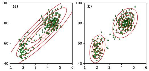
pp. 86–89 The Old Faithful data (272 eruptions: duration and waiting time) form two clumps, which a single Gaussian cannot represent (Figure 3.6(a)). A superposition of \(K\) Gaussians
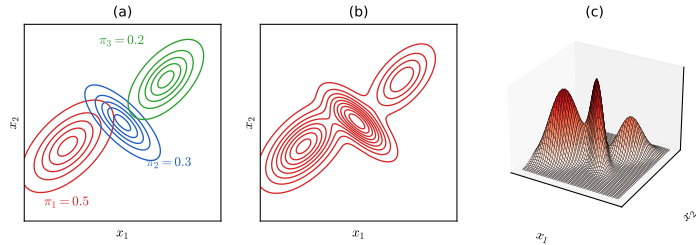
\[ p(\bx)=\sum_{k=1}^K\pi_k\N(\bx\given\bmu_k,\bSig_k) \tag{3.111} \]with mixing coefficients \(\sum_k\pi_k=1\) (3.112), \(0\le\pi_k\le1\) (3.113), can. Integrating (3.111) shows that (3.112) is necessary for normalisation; \(\pi_k\ge0\) is sufficient for \(p\ge0\) (and is imposed so that \(\pi_k=p(k)\) is a probability). By the sum and product rules \(p(\bx)=\sum_kp(k)p(\bx\given k)\) (3.114), and Bayes' theorem gives the responsibilities
\[ \gamma_k(\bx)\equiv p(k\given\bx)=\frac{\pi_k\N(\bx\given\bmu_k,\bSig_k)}{\sum_l\pi_l\N(\bx\given\bmu_l,\bSig_l)}. \tag{3.115} \]The log likelihood \(\ln p(\mathbf X\given\bpi,\bmu,\bSig)\)
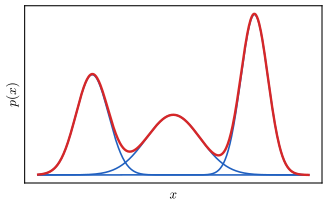
Note on Figure 3.7. The book labels the axes of this figure \(t\) and \(p(t\given x)\), the labels of a conditional density; the figure shows an ordinary (unconditional) density \(p(x)\).
Filling the gap 3.6: why the mixture likelihood is hard: stationarity, symmetry and singularities pp. 88–89
The book states that the mixture has "no closed-form analytical solution". Three precise facts lie behind this, and they recur for every latent-variable model in the book.
Derivation
Stationarity conditions are coupled. Differentiating (3.116) with respect to \(\bmu_k\), using \(\partial\N_k/\partial\bmu_k\)
Label switching. Permuting the \(K\) components leaves (3.116) unchanged, so every maximum comes with \(K!\) equivalent copies and the likelihood is not concave.
Unbounded likelihood. Put \(\bmu_k=\bx_1\) and \(\bSig_k=\sigma^2\bI\). The \(n=1\) term of (3.116) contains \(\pi_k(2\pi\sigma^2)^{-D/2}\), which tends to \(\infty\) as \(\sigma\to0\), while every other term stays bounded below by its other components. So \(\sup\ln p=+\infty\): the global maximum does not exist, and "maximum likelihood" for mixtures means a good local maximum away from these collapsed solutions (in practice, guarded by restarts or a small floor on the variances). The single Gaussian has no such problem when \(N>D\) (Filling the gap 3.4), because one component cannot sit on one point and still explain the others. ∎
3.3 Periodic Variables
See also: companion course, Section 2.3.8 Periodic variables.
pp. 89–90 Wind directions, times of day and dihedral angles of molecules are periodic: \(\theta\) and \(\theta+2\pi\) are the same point. Treating the numerical value of \(\theta\) as an ordinary variable makes the answer depend on the arbitrary origin. With two observations at \(1^\circ\) and \(359^\circ\), an origin at \(0^\circ\) gives a sample mean of \(180^\circ\) and standard deviation \(179^\circ\); an origin at \(180^\circ\) (so the values are \(181^\circ\) and \(179^\circ\)) gives \(0^\circ\) and \(1^\circ\). The cure is to represent \(\theta_n\) by the unit vector \(\bx_n=(\cos\theta_n,\sin\theta_n)\) and average those:
\[ \bar\bx=\frac1N\sum_{n=1}^N\bx_n, \tag{3.117} \] \[ \bar r\cos\bar\theta=\frac1N\sum_n\cos\theta_n,\qquad\bar r\sin\bar\theta=\frac1N\sum_n\sin\theta_n, \tag{3.118} \] \[ \bar\theta=\tan^{-1}\Big\{\frac{\sum_n\sin\theta_n}{\sum_n\cos\theta_n}\Big\}. \tag{3.119} \]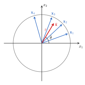
Filling the gap 3.7: the circular mean does not depend on the origin, and the right inverse tangent pp. 89–90
The book says the vector average "clearly" removes the dependence on the origin, and writes \(\tan^{-1}\) in (3.119), which needs care.
Derivation
Equivariance. Moving the origin by \(\alpha\) replaces every \(\theta_n\) by \(\theta_n-\alpha\), i.e. rotates every \(\bx_n\) by the rotation matrix \(\mathbf Q_{-\alpha}\). Averaging is linear, so \(\bar\bx\) is rotated by the same matrix: \(\bar r\) is unchanged and \(\bar\theta\) becomes \(\bar\theta-\alpha\). The mean direction is therefore the same physical direction whatever the origin, which is what "independent of the origin" means. The ordinary average lacks this property because the map \(\theta\mapsto\theta\bmod2\pi\) is not linear across the cut.
The inverse tangent. The ratio in (3.119) determines \(\bar\theta\) only modulo \(\pi\): \(\tan\) has period \(\pi\). The correct angle is the one for which \((\cos\bar\theta,\sin\bar\theta)\) has the signs of \((\sum_n\cos\theta_n,\sum_n\sin\theta_n)\), the two-argument function \(\bar\theta\)
3.3.1 Von Mises distribution
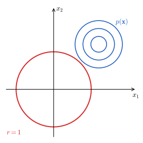
pp. 90–94 A density on the circle must satisfy \(p(\theta)\ge0\), \(\int_0^{2\pi}p(\theta)\,\d\theta=1\) and \(p(\theta+2\pi)=p(\theta)\) (3.120)–(3.122). Take an isotropic 2-D Gaussian with mean \(\bmu=(r_0\cos\theta_0,r_0\sin\theta_0)\) (3.125) and covariance \(\sigma^2\bI\),
\[ p(x_1,x_2)=\frac1{2\pi\sigma^2}\exp\Big\{-\frac{(x_1-\mu_1)^2+(x_2-\mu_2)^2}{2\sigma^2}\Big\}, \tag{3.123} \]write \(\bx\) in polar coordinates \(x_1=r\cos\theta\), \(x_2=r\sin\theta\) (3.124), and restrict to the unit circle \(r=1\) (Figure 3.10).
Result 3.12 (the von Mises distribution and its maximum likelihood estimates) pp. 91–93, (3.126)–(3.137)
On the unit circle the exponent of (3.123) is \(\frac{r_0}{\sigma^2}\cos(\theta\)
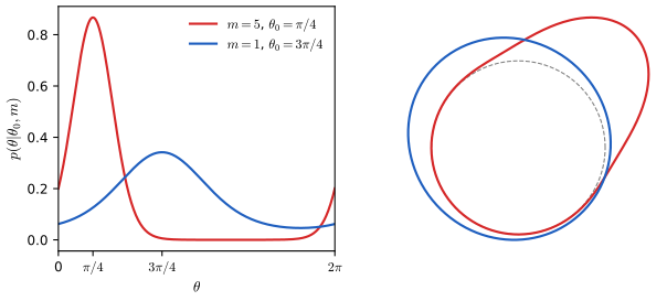
with mean direction \(\theta_0\) and concentration \(m\ge0\). For i.i.d. angles the log likelihood
\[ \ln p(\mathcal D\given\theta_0,m)=-N\ln(2\pi)-N\ln I_0(m)+m\sum_{n=1}^N\cos(\theta_n-\theta_0) \tag{3.131} \]is maximised by the circular mean and by the solution of \(A(m)=\bar r\):
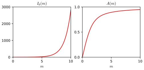
\[ \theta_0^{\rm ML}=\bar\theta,\qquad A(m_{\rm ML})=\frac1N\sum_{n=1}^N\cos(\theta_n-\theta_0^{\rm ML})=\bar r, \tag{3.134, 3.135} \] \[ A(m)=\frac{I_1(m)}{I_0(m)}. \tag{3.136} \]Proof (the exponent, normalisation and the stationary equations; Exercises 3.30, 3.32, 3.34)
(3.126). With \(r=1\), \((\cos\theta-r_0\cos\theta_0)^2\)
Normalisation. The substitution \(\theta\to\theta+\theta_0\) and periodicity give \(\int_0^{2\pi}e^{m\cos(\theta-\theta_0)}\d\theta\)
Mean direction. \(\partial/\partial\theta_0\) of (3.131) is \(m\sum_n\sin(\theta_n-\theta_0)\); setting it to zero (3.132) and expanding with \(\sin(A-B)=\sin A\cos B-\cos A\sin B\) (3.133) gives \(\cos\theta_0\sum_n\sin\theta_n\)
Concentration. With \(I_0'(m)=I_1(m)\) (differentiate (3.130) under the integral: \(I_0'(m)=\frac1{2\pi}\int\cos\theta\,e^{m\cos\theta}\d\theta\)
Filling the gap 3.8: \(A(m)=\bar r\) has a unique solution, Newton's method finds it, and the large-\(m\) limit pp. 92–93; Exercises 3.31, 3.33
The book says \(A(m)\) "can be inverted numerically" and that the distribution "becomes approximately Gaussian" for large \(m\). Both claims rest on properties of \(A\) that it does not prove.
Derivation
\(A\) is a mean and \(A'\) a variance. Under the von Mises density with \(\theta_0=0\), \(\E[\cos\theta]\)
Range. \(A(0)=0\) because \(I_1(0)=\frac1{2\pi}\int\cos\theta\,\d\theta\)
A closed form for \(A'\). \(\E[\cos^2\theta]=\frac{I_0''}{I_0}\), and from Bessel's equation \(I_0''+\frac1mI_0'-I_0=0\) we get \(I_0''=I_0-I_1/m\). Hence \(A'(m)=1-\frac{A(m)}m-A(m)^2\). Newton's method \(m\leftarrow m-(A(m)-\bar r)/A'(m)\) therefore needs only \(A\); because \(A\) is increasing and concave for \(m>0\) (concavity is a known property of the Bessel ratio, confirmed numerically on \([0,200]\)), each tangent lies above the curve, so after at most one step the iterates sit at or below the root and then increase monotonically to it; the code guards the first step against leaving \(m>0\) (it never moves below \(m/10\)), starts from Best and Fisher's approximation \(m_0=\bar r(2-\bar r^2)/(1-\bar r^2)\) and reaches machine precision in a few steps.
Maximum and minimum (Exercise 3.33). \(p'(\theta)\)
Gaussian limit (Exercise 3.31). Let \(\xi=m^{1/2}(\theta-\theta_0)\). Then \(m\cos(\theta-\theta_0)\)
Other periodic models. Mixtures of von Mises densities handle multimodal angles. Alternatives are histograms on the circle, densities obtained by marginalising (rather than conditioning) a 2-D Gaussian onto the circle, and wrapped densities \(\sum_{k\in\mathbb Z}p(\theta+2\pi k)\) obtained by winding the real line around the circle (Mardia and Jupp, 2000). All are periodic and normalised but less convenient than the von Mises distribution.
3.4 The Exponential Family
See also: companion course, Section 2.4 The exponential family and the toolkit's exponential families and moment matching.
Definition 3.3 (exponential family) p. 94, (3.138)–(3.139)
A family of distributions of the form
\[ p(\bx\given\bet)=h(\bx)\,g(\bet)\exp\{\bet^\T\bu(\bx)\} \tag{3.138} \]with natural parameters \(\bet\), sufficient statistic \(\bu(\bx)\), base measure \(h(\bx)\) and normaliser
\[ g(\bet)\int h(\bx)\exp\{\bet^\T\bu(\bx)\}\,\d\bx=1 \tag{3.139} \](a sum for discrete \(\bx\)). The natural parameter space is the set of \(\bet\) for which the integral is finite.
Result 3.13 (Bernoulli, multinomial and Gaussian in natural form) pp. 94–97, (3.140)–(3.167)
- Bernoulli. \(\Bern(x\given\mu)\)
\({}=(1-\mu)\exp\{x\ln\frac\mu{1-\mu}\}\) (3.141), so \(\eta=\ln\frac\mu{1-\mu}\) (3.142), \(\mu=\sigma(\eta)=\frac1{1+e^{-\eta}}\) (3.143), and \(p(x\given\eta)\) \({}=\sigma(-\eta)\exp(\eta x)\) (3.144): \(u(x)=x\), \(h=1\), \(g(\eta)=\sigma(-\eta)\) (3.145)–(3.147). - Multinomial, \(M\) parameters. \(p(\bx\given\bmu)\)
\({}=\exp\{\sum_kx_k\ln\mu_k\}\) \({}=\exp(\bet^\T\bx)\) with \(\eta_k=\ln\mu_k\), \(\bu(\bx)=\bx\), \(h=g=1\) (3.148)–(3.152), but the \(\eta_k\) are constrained by \(\sum_ke^{\eta_k}=1\) (3.153). - Multinomial, \(M-1\) free parameters. Eliminating \(\mu_M\) gives \(\eta_k=\ln\frac{\mu_k}{1-\sum_j\mu_j}\) (3.156), the softmax \(\mu_k=\frac{\exp(\eta_k)}{1+\sum_j\exp(\eta_j)}\) (3.157), and \(p(\bx\given\bet)\)
\({}=\big(1+\sum_{k=1}^{M-1}e^{\eta_k}\big)^{-1}\exp(\bet^\T\bx)\) (3.158)–(3.161), with \(\bet\) now unconstrained. - Gaussian. \(\bet=\begin{pmatrix}\mu/\sigma^2\\-1/(2\sigma^2)\end{pmatrix}\), \(\bu(x)=\begin{pmatrix}x\\x^2\end{pmatrix}\), \(h(x)=(2\pi)^{-1/2}\), \(g(\bet)=(-2\eta_2)^{1/2}\exp\Big(\frac{\eta_1^2}{4\eta_2}\Big)\) (3.164)–(3.167).
Proof (each identification, including the Gaussian's \(g\) and the softmax inversion)
Bernoulli. \(\mu^x(1-\mu)^{1-x}\)
Multinomial. Substitute \(x_M=1-\sum_{k<M}x_k\) and \(\mu_M=1-\sum_{k<M}\mu_k\) into \(\sum_kx_k\ln\mu_k\): \(\sum_{k<M}x_k\ln\mu_k+(1\)
Gaussian. Expanding, \(-\frac{(x-\mu)^2}{2\sigma^2}\)
Filling the gap 3.9: why the multinomial needs \(M-1\) parameters, and where the scale family (3.169) comes from pp. 95–97
Derivation
Identifiability. In the unconstrained \(M\)-parameter form, \(\exp(\bet^\T\bx)/\sum_ke^{\eta_k}\) is unchanged when a constant \(c\) is added to every \(\eta_k\), because \(\bx\) is one-hot (\(\bet^\T\bx\) and \(\ln\sum_ke^{\eta_k}\) both increase by \(c\)). So \(M\) unconstrained natural parameters describe the same distribution along a whole line: they are not identifiable, and the Hessian of the log likelihood is singular along \((1,\dots,1)\). Fixing \(\eta_M=0\) removes this direction, which is what (3.156)–(3.158) do. Softmax output layers in practice keep all \(M\) logits and live with this harmless redundancy (Chapter 5).
The scale family. If \(f\) is a density and \(s>0\), then \(\frac1sf(\frac xs)\) is a density, by the substitution \(y=x/s\) (\(\d x=s\,\d y\)) (3.168). Applying this to \(h(\bx)g(\bet)e^{\bet^\T\bx}\) with \(\bet=\boldsymbol\lambda_k\) (in \(D\) dimensions the factor is \(s^{-D}\), which the book's scalar formula leaves implicit) gives the class-conditional densities (3.169) with a shared scale; they are used in Chapter 5 to show that the posterior class probabilities of such models are a logistic sigmoid or softmax of a linear function of \(\bx\). ∎
3.4.1 Sufficient statistics
See also: companion course, Section 2.4.1 Maximum likelihood and sufficient statistics.
Result 3.14 (moments from \(g\); maximum likelihood is moment matching) pp. 97–98, (3.170)–(3.174), (3.218)
On the interior of the natural parameter space,
\[ -\nabla\ln g(\bet)=\E[\bu(\bx)], \tag{3.172} \] \[ -\nabla\nabla\ln g(\bet)=\E[\bu(\bx)\bu(\bx)^\T]-\E[\bu(\bx)]\E[\bu(\bx)^\T]=\cov[\bu(\bx)]. \tag{3.218} \]For i.i.d. data the likelihood \(\big(\prod_nh(\bx_n)\big)g(\bet)^N\exp\{\bet^\T\sum_n\bu(\bx_n)\}\) (3.173) depends on the data only through \(\sum_n\bu(\bx_n)\), and the maximum likelihood estimate satisfies
\[ -\nabla\ln g(\bet_{\rm ML})=\frac1N\sum_{n=1}^N\bu(\bx_n). \tag{3.174} \]Proof (differentiating the normaliser; Exercise 3.36)
Write \(Z(\bet)=1/g(\bet)\)
Filling the gap 3.10: when the moment-matching equation has exactly one solution, and in what sense \(\bet_{\rm ML}\to\bet\) p. 98
The book derives (3.174) as a stationarity condition and says that as \(N\to\infty\) "\(\bet_{\rm ML}\) will equal the true value". Here is what is true, and why.
Derivation
Differentiation under the integral. On the interior of the natural parameter space, for \(\bet\) in a small ball \(B\), \(\|\bu\|^ke^{\bet^\T\bu}\)
Concavity and uniqueness. By (3.218) the Hessian of the log likelihood is \(N\nabla\nabla\ln g=-N\cov[\bu]\), negative semidefinite: the log likelihood is concave in \(\bet\). If the representation is minimal (no nonzero \(\ba\) with \(\ba^\T\bu(\bx)\) almost surely constant, which fails for the \(M\)-parameter multinomial of Gap 3.9), \(\cov[\bu]\) is positive definite, the log likelihood is strictly concave, and (3.174) has at most one solution, which is then the global maximum. The mean map \(\bet\mapsto\E_{\bet}[\bu]\) is one-to-one in this case.
Existence. A solution exists iff the sample mean \(\bar\bu=\frac1N\sum_n\bu(\bx_n)\) lies in the interior of the convex hull of the possible values of \(\bu\). Example: for the Bernoulli, \(\sigma(\eta)=\bar x\) has no finite solution when all observations are 0 or all are 1 (Result 3.1's boundary case, \(\eta_{\rm ML}=\mp\infty\)).
Consistency. By the law of large numbers \(\bar\bu\to\E_{\bet^*}[\bu]\) almost surely under the true \(\bet^*\). The inverse of the mean map is continuous (inverse function theorem, its Jacobian \(\cov[\bu]\) being invertible), so \(\bet_{\rm ML}\to\bet^*\) almost surely. Moreover \(\sqrt N(\bet_{\rm ML}-\bet^*)\) is asymptotically \(\N(\mathbf0,\cov[\bu]^{-1})\), so the error shrinks like \(N^{-1/2}\): a simulation gives root-mean-square errors 0.50, 0.12, 0.047, 0.020 for the von Mises concentration at \(N=30,300,3000,30000\). "Equal to the true value" holds only in this limiting sense.
Moment matching as a projection. For any data distribution with \(\E[\bu]=\bar\bu\), \(\KL(\hat p\,\|\,p_{\bet})\)
Examples: the Bernoulli needs only \(\sum_nx_n\); the Gaussian needs \(\sum_nx_n\) and \(\sum_nx_n^2\), recovering the sufficient statistics (3.103) of Section 3.2.7; the von Mises with known \(\theta_0\) needs \(\sum_n\cos(\theta_n-\theta_0)\), and (3.174) reduces to \(A(m)=\bar r\).
3.5 Nonparametric Methods
See also: companion course, Section 2.5 Nonparametric methods and its density estimation demo (histograms, kernels and nearest neighbours with held-out likelihood).
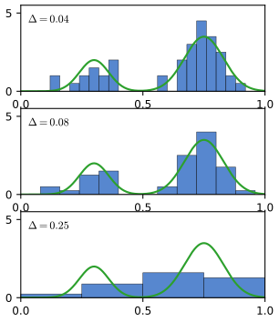
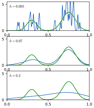
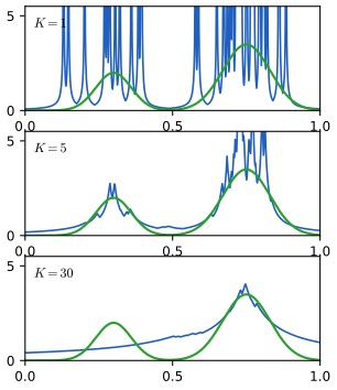
p. 98 A parametric family can be badly wrong (a single Gaussian for bimodal data). Nonparametric estimators make few assumptions about the shape of \(p\); their smoothing parameter controls complexity instead. The data of Figures 3.13–3.15 are 50 points from \(0.3\,\N(0.3,0.06^2)+0.7\,\N(0.75,0.08^2)\) (green curves).
3.5.1 Histograms
pp. 98–100 Partition the line into bins of widths \(\Delta_i\), count \(n_i\) points in bin \(i\), and set
\[ p_i=\frac{n_i}{N\Delta_i} \tag{3.175} \]on bin \(i\); then \(\int p\,\d x\)
3.5.2 Kernel densities
pp. 100–102 Let \(\mathcal R\) be a small region containing \(\bx\) with probability mass \(P=\int_{\mathcal R}p(\bx)\d\bx\) (3.176). The number \(K\) of the \(N\) points in \(\mathcal R\) is \(\Bin(K\given N,P)\) (3.177), so \(\E[K/N]=P\) and \(\var[K/N]=P(1-P)/N\). For large \(N\), \(K\simeq NP\) (3.178); for small \(\mathcal R\) of volume \(V\), \(P\simeq p(\bx)V\) (3.179). Together
\[ p(\bx)\simeq\frac K{NV}. \tag{3.180} \]Fixing \(V\) and counting \(K\) gives kernel estimators; fixing \(K\) and measuring \(V\) gives nearest neighbours. With the unit-cube Parzen window \(k(\bu)=1\) if \(|u_i|\le\frac12\) for all \(i\), else 0 (3.181), the count in the cube of side \(h\) around \(\bx\) is \(K=\sum_nk((\bx-\bx_n)/h)\) (3.182), and
\[ p(\bx)=\frac1N\sum_{n=1}^N\frac1{h^D}k\Big(\frac{\bx-\bx_n}h\Big), \tag{3.183} \]or, with a Gaussian kernel of standard deviation \(h\),
\[ p(\bx)=\frac1N\sum_{n=1}^N\frac1{(2\pi h^2)^{D/2}}\exp\Big\{-\frac{\|\bx-\bx_n\|^2}{2h^2}\Big\}. \tag{3.184} \]Any kernel with \(k(\bu)\ge0\) and \(\int k(\bu)\d\bu=1\) (3.185)–(3.186) gives a valid density, because each term \(h^{-D}k((\bx-\bx_n)/h)\) integrates to 1 (substitute \(\bu=(\bx-\bx_n)/h\)). There is no training, but evaluating the density costs \(O(N)\).
Filling the gap 3.11: the bias and variance of a kernel density estimate, and the rate at which \(h\) must shrink p. 101
The book notes that (3.180) rests on "two contradictory assumptions" and that the estimators converge "provided that \(V\) shrinks with \(N\) and \(K\) grows with \(N\), at an appropriate rate". The bias–variance calculation makes both statements precise.
Derivation
Let \(k_h(\bx)=h^{-D}k(\bx/h)\) with a symmetric kernel, \(\int\bu\,k=\mathbf0\), \(\int u_iu_jk=\kappa_2\delta_{ij}\), \(R(k)=\int k^2\). The estimate \(\hat p(\bx)=\frac1N\sum_nk_h(\bx-\bx_n)\) is an average of i.i.d. terms.
Mean. \(\E[\hat p(\bx)]\)
Variance. \(\var[\hat p(\bx)]\)
Trade-off. The mean squared error is about \(\frac{h^4}4\kappa_2^2(\nabla^2p)^2\)
3.5.3 Nearest-neighbours
pp. 103–105 A fixed \(h\) over-smooths where data are dense and is noisy where they are sparse. The \(K\)-nearest-neighbour estimate grows a sphere around \(\bx\) until it holds \(K\) points and uses its volume \(V\) in (3.180). \(K\) now controls the smoothing (Figure 3.15). The result is not a density: its integral over the whole space diverges (Exercise 3.38).
Result 3.15 (the \(K\)-nearest-neighbour classifier) pp. 103–104, (3.187)–(3.190)
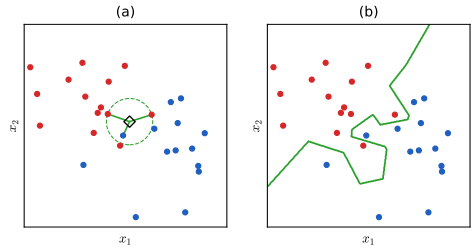
With \(N_k\) training points in class \(\mathcal C_k\), draw the sphere around \(\bx\) holding \(K\) points in total, of which \(K_k\) are in \(\mathcal C_k\). The estimates \(p(\bx\given\mathcal C_k)\)
so the minimum-misclassification rule assigns \(\bx\) to the majority class among its \(K\) nearest neighbours.
Proof
\(\frac{K_k}{N_kV}\cdot\frac{N_k}N\Big/\frac K{NV}\)
Filling the gap 3.12: why the 1-NN boundary consists of bisectors, and the Cover–Hart bound p. 104
The book states both facts in a figure caption and a sentence. The companion course proves the bound in full (Result 2.28); here is the argument in brief.
Derivation
Bisectors. The set of points closer to \(\bx_i\) than to \(\bx_j\) is \(\{\bx:\|\bx-\bx_i\|^2\)
Cover–Hart bound (two classes). Let \(\eta(\bx)=p(\mathcal C_1\given\bx)\). The Bayes error is \(R^*=\E[\min(\eta,1-\eta)]\). As \(N\to\infty\) the nearest neighbour \(\bx'\) of \(\bx\) converges to \(\bx\), and if \(\eta\) is continuous its label is an independent draw with the same probabilities. The 1-NN rule errs when the two labels differ, with probability \(2\eta(1-\eta)\). With \(m=\min(\eta,1-\eta)\), \(2\eta(1-\eta)=2m(1-m)\), so \(R_{\rm NN}\)
Both kernel and nearest-neighbour methods store all \(N\) training points and spend \(O(N)\) per query (tree-based search structures help, at some set-up cost). Parametric models are cheap but rigid. The book's answer, developed from Chapter 4 on, is a model with a large but fixed number of parameters whose flexibility does not depend on \(N\): a deep neural network.
Exercises
All 38 exercises of Chapter 3 (Bishop and Bishop, 2024, pp. 105–110), restated in my own words, with complete solutions (hidden). Stars give the book's difficulty. Each was solved independently and then compared with the official solutions manual (version 1.0); the places where the manual is wrong are flagged and summarised in the box after the list, and the key ones are confirmed numerically.
Exercise 3.1 (★). Check that the Bernoulli distribution (3.2) sums to 1, has mean \(\mu\) and variance \(\mu(1-\mu)\), and has entropy \(\mathrm H[x]\)
\({}=-\mu\ln\mu-(1-\mu)\ln(1-\mu)\). Solution
Normalisation, mean and variance: the proof under Definition 3.1. Entropy: \(\mathrm H\)
\({}=-\sum_xp(x)\ln p(x)\) \({}=-(1-\mu)\ln(1-\mu)-\mu\ln\mu\). It is maximal, \(\ln2\), at \(\mu=\frac12\), and 0 at \(\mu\in\{0,1\}\). Exercise 3.2 (★★). For \(x\in\{-1,1\}\) let \(p(x\given\mu)\)
\({}=\big(\frac{1-\mu}2\big)^{(1-x)/2}\big(\frac{1+\mu}2\big)^{(1+x)/2}\) with \(\mu\in[-1,1]\) (3.195). Show it is normalised and find its mean, variance and entropy. Solution
\(p(1)=\frac{1+\mu}2\), \(p(-1)=\frac{1-\mu}2\), sum 1. \(\E[x]=\frac{1+\mu}2-\frac{1-\mu}2=\mu\); \(x^2=1\) so \(\var[x]=1-\mu^2\). \(\mathrm H\)
\({}=-\frac{1-\mu}2\ln\frac{1-\mu}2\) \({}-\frac{1+\mu}2\ln\frac{1+\mu}2\). (It is the ordinary Bernoulli for \(y=(1+x)/2\) with parameter \((1+\mu)/2\).) Exercise 3.3 (★★). Prove \(\binom Nm+\binom N{m-1}=\binom{N+1}m\) (3.196), use it to prove the binomial theorem \((1+x)^N=\sum_{m=0}^N\binom Nmx^m\) (3.197) by induction, and deduce that the binomial distribution is normalised (3.198).
Solution
Pascal's rule. \(\frac{N!}{m!(N-m)!}+\frac{N!}{(m-1)!(N-m+1)!}\)
\({}=\frac{N!\{(N-m+1)+m\}}{m!(N-m+1)!}\) \({}=\frac{(N+1)!}{m!(N+1-m)!}\). Induction. True for \(N=0\). If true for \(N\): \((1+x)^{N+1}\)
\({}=\sum_m\binom Nmx^m+\sum_m\binom Nmx^{m+1}\) \({}=\sum_{m=0}^{N+1}\big\{\binom Nm\) \({}+\binom N{m-1}\big\}x^m\) (with \(\binom N{-1}=\binom N{N+1}=0\)) \(=\sum_m\binom{N+1}mx^m\). Normalisation. \(\sum_m\binom Nm\mu^m(1-\mu)^{N-m}\)
\({}=(1-\mu)^N\sum_m\binom Nm\big(\frac\mu{1-\mu}\big)^m\) \({}=(1-\mu)^N\big(1+\frac\mu{1-\mu}\big)^N\) \({}=1\) (for \(\mu<1\); \(\mu=1\) is immediate). Exercise 3.4 (★★). Obtain the binomial mean (3.11) by differentiating the normalisation condition (3.198) with respect to \(\mu\), and the variance (3.12) by differentiating twice. (The book's wording says "the mean of \(n\)"; it means \(m\).)
Solution
Given in the second part of the proof of Result 3.2. The key fact is \(\frac{\d}{\d\mu}\Bin(m\given N,\mu)\)
\({}=\Bin(m\given N,\mu)\frac{m-N\mu}{\mu(1-\mu)}\); one differentiation gives \(\E[m-N\mu]=0\), a second gives \(\E[(m-N\mu)^2]=N\mu(1-\mu)\). Exercise 3.5 (★). Show that the mode of \(\N(\bx\given\bmu,\bSig)\) is \(\bmu\).
Solution
The density is a decreasing function of \(\Delta^2\)
\({}=(\bx-\bmu)^\T\bSig^{-1}(\bx-\bmu)\) \({}\ge0\), and \(\Delta^2=0\) only at \(\bx=\bmu\) (positive definiteness), so \(\bmu\) is the unique maximiser. Equivalently \(\nabla\N=-\N\,\bSig^{-1}(\bx-\bmu)\) vanishes only at \(\bmu\). Exercise 3.6 (★★). If \(\bx\sim\N(\bmu,\bSig)\), show that \(\mathbf y=\bA\bx+\bb\) is Gaussian and find its mean and covariance.
Solution
Mean \(\bA\bmu+\bb\) and covariance \(\E[\bA(\bx-\bmu)(\bx-\bmu)^\T\bA^\T]\)
\({}=\bA\bSig\bA^\T\), by linearity. Gaussianity for any \(K\times D\) matrix \(\bA\): the characteristic function is \(\E[e^{i\mathbf t^\T\by}]\) \({}=e^{i\mathbf t^\T\bb}\E[e^{i(\bA^\T\mathbf t)^\T\bx}]\) \({}=\exp\{i\mathbf t^\T(\bA\bmu\) \({}+\bb)-\frac12\mathbf t^\T\bA\bSig\bA^\T\mathbf t\}\), the characteristic function of \(\N(\bA\bmu+\bb,\bA\bSig\bA^\T)\) (singular if \(\bA\) has rank below \(K\)). For square invertible \(\bA\) one can also change variables: \(p_{\by}(\by)\) \({}=p_{\bx}(\bA^{-1}(\by-\bb))/|\det\bA|\), whose exponent is \(-\frac12(\by-\bA\bmu-\bb)^\T(\bA\bSig\bA^\T)^{-1}(\by\) \({}-\bA\bmu-\bb)\). Manual: its solution assumes \(\bA\) square, symmetric and invertible and gives the covariance as \(\bA\bSig\bA\), which is correct only for symmetric \(\bA\); the general answer is \(\bA\bSig\bA^\T\) (checked numerically with a non-symmetric \(\bA\)). Exercise 3.7 (★★★). Show that \(\KL(\N(\bmu_q,\bSig_q)\,\|\,\N(\bmu_p,\bSig_p))\)
\({}=\frac12\big\{\ln\frac{|\bSig_p|}{|\bSig_q|}\) \({}-D+\Tr(\bSig_p^{-1}\bSig_q)\) \({}+(\bmu_p-\bmu_q)^\T\bSig_p^{-1}(\bmu_p\) \({}-\bmu_q)\big\}\) (3.199). Solution
\(\KL=\E_q[\ln q-\ln p]\). With \(\ln\N(\bx\given\bmu,\bSig)\)
\({}=-\frac D2\ln2\pi-\frac12\ln|\bSig|\) \({}-\frac12(\bx-\bmu)^\T\bSig^{-1}(\bx\) \({}-\bmu)\) and the identity \(\E_q[(\bx-\mathbf a)^\T\bM(\bx\) \({}-\mathbf a)]\) \({}=\Tr(\bM\bSig_q)+(\bmu_q\) \({}-\mathbf a)^\T\bM(\bmu_q-\mathbf a)\) (expand around \(\bmu_q\); the cross term has zero mean): \(\E_q[\ln q]\) \({}=-\frac D2\ln2\pi-\frac12\ln|\bSig_q|\) \({}-\frac D2\) and \(\E_q[\ln p]\) \({}=-\frac D2\ln2\pi-\frac12\ln|\bSig_p|\) \({}-\frac12\Tr(\bSig_p^{-1}\bSig_q)\) \({}-\frac12(\bmu_q-\bmu_p)^\T\bSig_p^{-1}(\bmu_q\) \({}-\bmu_p)\). Subtracting gives (3.199). (Checked by Monte Carlo: 1.0202 against 1.0195.) Exercise 3.8 (★★). Maximise the entropy \(\mathrm H[\bx]=-\int p\ln p\) (3.200) subject to normalisation and a given mean \(\bmu\) and covariance \(\bSig\) (3.201)–(3.203), using Lagrange multipliers, and show that the maximiser is the Gaussian (3.26). (The book's last sentence says "maximum likelihood distribution"; it means maximum entropy.)
Solution
Stationarity. With multipliers \(\lambda\), \(\mathbf m\) and a symmetric matrix \(\bL\), the functional derivative of \(-\int p\ln p+\lambda(\int p\)
\({}-1)+\mathbf m^\T(\int p\bx\) \({}-\bmu)+\Tr\{\bL(\int p(\bx\) \({}-\bmu)(\bx-\bmu)^\T-\bSig)\}\) is \(-\ln p-1+\lambda+\mathbf m^\T\bx\) \({}+(\bx-\bmu)^\T\bL(\bx-\bmu)\); setting it to zero gives \(p(\bx)=\exp\{\lambda-1+\mathbf m^\T\bx\) \({}+(\bx-\bmu)^\T\bL(\bx-\bmu)\}\), the exponential of a quadratic. Integrability needs \(\bL\) negative definite, so \(p\) is a Gaussian; matching its mean and covariance to the constraints forces \(\mathbf m=\mathbf0\) and \(\bL=-\frac12\bSig^{-1}\), and \(\lambda\) is fixed by normalisation. It is the maximum. For any \(q\) with the same mean and covariance, \(\int q\ln\N=\int\N\ln\N\) (\(\ln\N\) is a quadratic, whose expectation depends only on the first two moments), so \(\mathrm H[\N]-\mathrm H[q]\)
\({}=\KL(q\,\|\,\N)\) \({}\ge0\). Manual: it states \(\bL=-\frac12\bSig\); the correct value is \(-\frac12\bSig^{-1}\). Exercise 3.9 (★★★). Show that \(\mathrm H[\N(\bmu,\bSig)]\)
\({}=\frac12\ln|\bSig|+\frac D2(1+\ln2\pi)\) (3.204). Solution
\(-\E[\ln\N]\)
\({}=\frac D2\ln2\pi+\frac12\ln|\bSig|\) \({}+\frac12\E[\Delta^2]\) and \(\E[\Delta^2]\) \({}=\Tr(\bSig^{-1}\E[(\bx-\bmu)(\bx\) \({}-\bmu)^\T])\) \({}=\Tr\bI=D\). Exercise 3.10 (★★★). \(x_1\) and \(x_2\) are independent Gaussians with means \(\mu_1,\mu_2\) and precisions \(\tau_1,\tau_2\). Find the entropy of \(x=x_1+x_2\) by computing \(p(x)=\int p(x\given x_2)p(x_2)\d x_2\) (3.205).
Solution
\(p(x\given x_2)\)
\({}=\N(x\given\mu_1+x_2,\tau_1^{-1})\). The exponent of the integrand is \(-\frac{\tau_1}2(x-\mu_1-x_2)^2\) \({}-\frac{\tau_2}2(x_2-\mu_2)^2\). Completing the square in \(x_2\): the \(x_2\) terms are \(-\frac{\tau_1+\tau_2}2x_2^2\) \({}+x_2\{\tau_1(x-\mu_1)+\tau_2\mu_2\}\); integrating out leaves \(\frac{\{\tau_1(x-\mu_1)+\tau_2\mu_2\}^2}{2(\tau_1+\tau_2)}\) \({}-\frac{\tau_1}2(x-\mu_1)^2\) \({}+\const\), whose \(x^2\) coefficient is \(-\frac12\big(\tau_1-\frac{\tau_1^2}{\tau_1+\tau_2}\big)\) \({}=-\frac12\frac{\tau_1\tau_2}{\tau_1+\tau_2}\). So \(x\sim\N(\mu_1+\mu_2,\tau_1^{-1}\) \({}+\tau_2^{-1})\) (as also follows from (3.99)) and \(\mathrm H[x]\) \({}=\frac12\ln\{2\pi e(\tau_1^{-1}\) \({}+\tau_2^{-1})\}\). Exercise 3.11 (★). Show that the antisymmetric part of the precision matrix drops out of the exponent of the Gaussian, so the precision (and hence the covariance) can be taken symmetric.
Solution
Write \(\bLam=\bLam^S+\bLam^A\) with \(\bLam^S=\frac12(\bLam+\bLam^\T)\), \(\bLam^A=\frac12(\bLam-\bLam^\T)\). A scalar equals its transpose, so \(\ba^\T\bLam^A\ba\)
\({}=\ba^\T(\bLam^A)^\T\ba\) \({}=-\ba^\T\bLam^A\ba\) \({}=0\). The covariance is then the inverse of a symmetric matrix, symmetric by Exercise 3.16. Exercise 3.12 (★★★). For real symmetric \(\bSig\), show that the eigenvalues are real, that eigenvectors of distinct eigenvalues are orthogonal, and that an orthonormal set of eigenvectors can always be chosen, even with zero (or repeated) eigenvalues.
Solution
See the proof of Result 3.4. Orthogonality needs only \(\lambda_i\ne\lambda_j\), zero eigenvalues included. (The manual assumes nonzero eigenvalues for this step, which is unnecessary, and handles repeated eigenvalues only for pairs; the induction in Result 3.4 covers every multiplicity.)
Exercise 3.13 (★★). Show that \(\bSig=\sum_i\lambda_i\bu_i\bu_i^\T\) (3.31) and \(\bSig^{-1}\)
\({}=\sum_i\lambda_i^{-1}\bu_i\bu_i^\T\) (3.32). Solution
Both sides of (3.31) act identically on the basis \(\{\bu_j\}\): \(\big(\sum_i\lambda_i\bu_i\bu_i^\T\big)\bu_j\)
\({}=\lambda_j\bu_j\) \({}=\bSig\bu_j\), so they are equal. Multiplying the two sums gives \(\sum_{i,j}\frac{\lambda_i}{\lambda_j}\bu_i(\bu_i^\T\bu_j)\bu_j^\T\) \({}=\sum_i\bu_i\bu_i^\T\) \({}=\bI\) (completeness of an orthonormal basis). Exercise 3.14 (★★). Show that a symmetric \(\bSig\) is positive definite (\(\ba^\T\bSig\ba>0\) for all real \(\ba\ne\mathbf0\), (3.206)) iff all its eigenvalues are positive.
Solution
Expand \(\ba=\sum_i\hat a_i\bu_i\): \(\ba^\T\bSig\ba\)
\({}=\sum_i\lambda_i\hat a_i^2\). If all \(\lambda_i>0\) this is positive whenever some \(\hat a_i\ne0\), i.e. whenever \(\ba\ne\mathbf0\). If some \(\lambda_j\le0\), \(\ba=\bu_j\) gives \(\lambda_j\le0\). (The manual's final sentence says "eigenvectors" where it means eigenvalues.) Exercise 3.15 (★). Show that a real symmetric \(D\times D\) matrix has \(D(D+1)/2\) independent parameters.
Solution
The entries on and above the diagonal determine the matrix and can be chosen freely: \(D+(D^2-D)/2=D(D+1)/2\).
Exercise 3.16 (★). Show that the inverse of a symmetric matrix is symmetric.
Solution
Transpose \(\bM\bM^{-1}=\bI\): \((\bM^{-1})^\T\bM^\T=\bI\), i.e. \((\bM^{-1})^\T\bM=\bI\), so \((\bM^{-1})^\T\) is the (unique) inverse \(\bM^{-1}\).
Exercise 3.17 (★★). Show that the volume inside the hyperellipsoid of constant Mahalanobis distance \(\Delta\) is \(V_D|\bSig|^{1/2}\Delta^D\) (3.207), with \(V_D\) the volume of the unit ball.
Solution
The rotation \(\by=\bU(\bx-\bmu)\) preserves volume and turns the region into \(\sum_iy_i^2/\lambda_i\le\Delta^2\). Put \(y_i=\lambda_i^{1/2}z_i\): the region becomes the ball \(\|\mathbf z\|\le\Delta\), of volume \(V_D\Delta^D\), and the Jacobian is \(\prod_i\lambda_i^{1/2}=|\bSig|^{1/2}\). (The manual writes the substitution as \(z_i=\lambda_i^{1/2}y_i\), which is the wrong direction; its final answer is right. Checked by Monte Carlo in 2 and 3 dimensions.)
Exercise 3.18 (★★). Prove the partitioned inverse formula (3.60) by multiplying by the original matrix (3.208).
Solution
The four block products are worked out in the proof of Result 3.8.
Exercise 3.19 (★★★). Partition \(\bx\) into three groups \(\bx_a,\bx_b,\bx_c\) (3.209). Find \(p(\bx_a\given\bx_b)\) with \(\bx_c\) marginalised out.
Solution
First marginalise (Result 3.9): \(p(\bx_a,\bx_b)\) is Gaussian with mean \((\bmu_a,\bmu_b)\) and covariance \(\begin{pmatrix}\bSig_{aa}&\bSig_{ab}\\\bSig_{ba}&\bSig_{bb}\end{pmatrix}\): just delete the \(c\) rows and columns. Then condition (Result 3.7): \(p(\bx_a\given\bx_b)\)
\({}=\N(\bx_a\given\bmu_a+\bSig_{ab}\bSig_{bb}^{-1}(\bx_b\) \({}-\bmu_b),\;\bSig_{aa}-\bSig_{ab}\bSig_{bb}^{-1}\bSig_{ba})\). In covariance form the presence of \(\bx_c\) is invisible; in precision form it is not, because the precision of the \((a,b)\) marginal is not a sub-block of \(\bLam\). (The manual's last sentence calls the result "\(p(\bx_a,\bx_b)\)"; it means \(p(\bx_a\given\bx_b)\). Checked by a Monte Carlo regression.) Exercise 3.20 (★★). Prove the Woodbury identity \((\bA+\mathbf B\mathbf C\mathbf D)^{-1}\)
\({}=\bA^{-1}-\bA^{-1}\mathbf B(\mathbf C^{-1}\) \({}+\mathbf D\bA^{-1}\mathbf B)^{-1}\mathbf D\bA^{-1}\) (3.210). Solution
Multiply the right side on the left by \(\bA+\mathbf B\mathbf C\mathbf D\): \(\bI+\mathbf B\mathbf C\mathbf D\bA^{-1}\)
\({}-\mathbf B(\bI+\mathbf C\mathbf D\bA^{-1}\mathbf B)(\mathbf C^{-1}\) \({}+\mathbf D\bA^{-1}\mathbf B)^{-1}\mathbf D\bA^{-1}\). Since \(\bI+\mathbf C\mathbf D\bA^{-1}\mathbf B\) \({}=\mathbf C(\mathbf C^{-1}\) \({}+\mathbf D\bA^{-1}\mathbf B)\), the last term is \(\mathbf B\mathbf C\mathbf D\bA^{-1}\), and everything cancels to \(\bI\). See also the companion toolkit's Woodbury entry. Exercise 3.21 (★). For independent \(\bx\) and \(\bz\), show that \(\by=\bx+\bz\) has mean \(\E\bx+\E\bz\) and covariance \(\cov\bx+\cov\bz\).
Solution
Linearity gives the mean. \(\cov[\by]\)
\({}=\E[(\tilde\bx+\tilde\bz)(\tilde\bx\) \({}+\tilde\bz)^\T]\) with centred \(\tilde\bx,\tilde\bz\); the cross terms \(\E[\tilde\bx\tilde\bz^\T]\) \({}=\E[\tilde\bx]\E[\tilde\bz]^\T\) \({}=\mathbf0\) by independence. (The manual writes \(\by\) where it means \(\bz\) inside the expansion.) Exercise 3.22 (★★★). From the joint mean (3.92) and covariance (3.89), recover \(p(\bx)\) (3.83) by marginalisation and \(p(\by\given\bx)\) (3.84) by conditioning.
Solution
Marginal of \(\bx\): top blocks, \(\N(\bmu,\bLam^{-1})\). Conditional by (3.65)–(3.66) with \(a=\by\), \(b=\bx\): mean \(\bA\bmu+\bb+\bA\bLam^{-1}\bLam(\bx-\bmu)\)
\({}=\bA\bx+\bb\); covariance \(\bL^{-1}+\bA\bLam^{-1}\bA^\T\) \({}-\bA\bLam^{-1}\bLam\bLam^{-1}\bA^\T\) \({}=\bL^{-1}\). Exercise 3.23 (★★). Use (3.60) to show that the inverse of \(\bR\) in (3.88) is (3.89).
Solution
Worked in the proof of Result 3.10: the Schur complement of \(\bL\) in \(\bR\) is \(\bLam\).
Exercise 3.24 (★★). Verify (3.92) from (3.91) and (3.89).
Solution
Worked in the proof of Result 3.10: the blocks are \(\bmu\) and \(\bA\bmu+\bb\). (The manual's final line has \(\bA\bmu-\bb\), a sign slip, and writes \(\mathbf S\) for \(\bL\).)
Exercise 3.25 (★★). With \(\bx\sim\N(\bmu_x,\bSig_x)\) and independent \(\bz\sim\N(\bmu_z,\bSig_z)\), use the linear-Gaussian results to show \(\by=\bx+\bz\)
\({}\sim\N(\bmu_x+\bmu_z,\bSig_x+\bSig_z)\) (3.212). Solution
\(p(\by\given\bx)\)
\({}=\N(\by\given\bx+\bmu_z,\bSig_z)\): the model (3.83)–(3.84) with \(\bA=\bI\), \(\bb=\bmu_z\), \(\bL^{-1}=\bSig_z\), \(\bLam^{-1}=\bSig_x\). Then (3.99) gives mean \(\bmu_x+\bmu_z\) and covariance \(\bSig_z+\bSig_x\). Exercise 3.26 (★★★). For the joint defined by (3.83)–(3.84), complete the square to integrate out \(\bx\), and use Woodbury to recover the mean and covariance (3.93)–(3.94) of \(p(\by)\).
Solution
The exponent's \(\bx\) terms are \(-\frac12\bx^\T\bS^{-1}\bx\)
\({}+\bx^\T\mathbf c\) with \(\bS=(\bLam+\bA^\T\bL\bA)^{-1}\), \(\mathbf c=\bLam\bmu+\bA^\T\bL(\by-\bb)\). Integrating out \(\bx\) leaves \(\frac12\mathbf c^\T\bS\mathbf c\), plus the remaining terms \(-\frac12(\by-\bb)^\T\bL(\by-\bb)\). The quadratic term in \(\by\) is \(-\frac12\by^\T(\bL-\bL\bA\bS\bA^\T\bL)\by\), and by Woodbury (with \(\bA\to\bL^{-1}\), \(\mathbf B\to\bA\), \(\mathbf C\to\bLam^{-1}\), \(\mathbf D\to\bA^\T\)) \((\bL^{-1}+\bA\bLam^{-1}\bA^\T)^{-1}\) \({}=\bL-\bL\bA(\bLam+\bA^\T\bL\bA)^{-1}\bA^\T\bL\), so the covariance is \(\bL^{-1}+\bA\bLam^{-1}\bA^\T\). The linear term is \(\by^\T\{(\bL-\bL\bA\bS\bA^\T\bL)\bb\) \({}+\bL\bA\bS\bLam\bmu\}\); multiplying by the covariance, the first part gives \(\bb\), and \((\bL^{-1}+\bA\bLam^{-1}\bA^\T)\bL\bA\bS\bLam\bmu\) \({}=\bA(\bI+\bLam^{-1}\bA^\T\bL\bA)\bS\bLam\bmu\) \({}=\bA\bLam^{-1}(\bLam+\bA^\T\bL\bA)\bS\bLam\bmu\) \({}=\bA\bmu\). Mean \(\bA\bmu+\bb\). (Both checked numerically.) Exercise 3.27 (★★★). For the same joint, complete the square in \(\bx\) to find \(p(\bx\given\by)\), and check (3.95)–(3.96).
Solution
Done in Filling the gap 3.3: precision \(\bLam+\bA^\T\bL\bA\), mean \((\bLam+\bA^\T\bL\bA)^{-1}\{\bLam\bmu\)
\({}+\bA^\T\bL(\by-\bb)\}\). (The manual's first line has \(\bA\bL\) where \(\bA^\T\bL\) is meant.) Exercise 3.28 (★★). Maximise (3.102) over \(\bSig\), ignoring the symmetry and positive-definiteness constraints, and show the result is the sample covariance (3.106).
Solution
The gradient \(\frac N2(\bSig^{-1}\bS\bSig^{-1}\)
\({}-\bSig^{-1})\) vanishes at \(\bSig=\bS\). Filling the gap 3.4 gives this computation and a complete proof that \(\bS\) is the global maximum over positive definite matrices, so the constraints never had to be ignored. Exercise 3.29 (★★). Prove \(\E[\bx_n\bx_m^\T]\)
\({}=\bmu\bmu^\T+I_{nm}\bSig\) (3.213) for independent draws and deduce (3.108). Solution
In the proof of Result 3.11. (Checked by simulation: the average of \(\bSig_{\rm ML}\) over 40 000 data sets of size 5 is \(0.8\bSig\) to within 0.005.)
Exercise 3.30 (★). Prove \(\cos^2A+\sin^2A=1\), \(\cos(A-B)=\cos A\cos B+\sin A\sin B\) and \(\sin(A-B)=\sin A\cos B-\cos A\sin B\) from \(e^{iA}=\cos A+i\sin A\) (3.214).
Solution
\(1=e^{iA}e^{-iA}\)
\({}=(\cos A+i\sin A)(\cos A-i\sin A)\) \({}=\cos^2A+\sin^2A\). \(e^{i(A-B)}\) \({}=(\cos A+i\sin A)(\cos B-i\sin B)\) \({}=(\cos A\cos B+\sin A\sin B)\) \({}+i(\sin A\cos B-\cos A\sin B)\); the real and imaginary parts are the two formulas. Exercise 3.31 (★★). With \(\xi=m^{1/2}(\theta-\theta_0)\) and \(\cos\alpha=1-\alpha^2/2+O(\alpha^4)\) (3.217), show that the von Mises distribution tends to a Gaussian as \(m\to\infty\).
Solution
\(m\cos(\xi/\sqrt m)=m-\xi^2/2+O(\xi^4/m)\), so \(p(\xi)\propto e^{-\xi^2/2}\) in the limit, i.e. \(\theta\approx\N(\theta_0,1/m)\). The normaliser and the error are treated in Filling the gap 3.8.
Exercise 3.32 (★). Use (3.133) to solve (3.132) for \(\theta_0\).
Solution
\(\sum_n\sin(\theta_n-\theta_0)\)
\({}=\cos\theta_0\sum_n\sin\theta_n\) \({}-\sin\theta_0\sum_n\cos\theta_n\) \({}=0\), so \(\tan\theta_0\) \({}=\sum_n\sin\theta_n/\sum_n\cos\theta_n\). Of the two solutions modulo \(2\pi\), the maximum is the one in the quadrant of \((\sum\cos,\sum\sin)\) (Filling the gap 3.7). Exercise 3.33 (★). Using the first and second derivatives of (3.129), show that the von Mises density is maximal at \(\theta_0\) and minimal at \(\theta_0+\pi\).
Solution
\(p'=-m\sin(\theta-\theta_0)p\), zero at \(\theta_0\) and \(\theta_0+\pi\); \(p''=m\{m\sin^2(\theta-\theta_0)\)
\({}-\cos(\theta-\theta_0)\}p\), equal to \(-mp<0\) at \(\theta_0\) and \(+mp>0\) at \(\theta_0+\pi\) (for \(m>0\)). Manual: its \(p'\) omits the factor \(m\) and its \(p''\) is \(-p\{\sin^2+\cos\}\), which has neither factor \(m\) nor the right sign on \(\sin^2\); since \(\sin=0\) at both stationary points the conclusion survives (checked against finite differences). Exercise 3.34 (★). Show that \(m_{\rm ML}\) satisfies \(A(m_{\rm ML})=\bar r\).
Solution
By (3.118), \(\frac1N\sum_n\cos\theta_n\)
\({}=\bar r\cos\bar\theta\) and \(\frac1N\sum_n\sin\theta_n\) \({}=\bar r\sin\bar\theta\). With \(\theta_0^{\rm ML}=\bar\theta\), the right side of (3.137) is \(\bar r(\cos^2\bar\theta+\sin^2\bar\theta)\) \({}=\bar r\). Exercise 3.35 (★). Write the multivariate Gaussian in exponential-family form and find \(\bet\), \(\bu(\bx)\), \(h(\bx)\), \(g(\bet)\).
Solution
The exponent is \(-\frac12\Tr(\bSig^{-1}\bx\bx^\T)\)
\({}+\bx^\T\bSig^{-1}\bmu-\frac12\bmu^\T\bSig^{-1}\bmu\). So \(\bu(\bx)\) \({}=(\bx,\operatorname{vec}(\bx\bx^\T))\), \(\bet=(\bet_1,\operatorname{vec}\bet_2)\) with \(\bet_1=\bSig^{-1}\bmu\), \(\bet_2=-\frac12\bSig^{-1}\), \(h=(2\pi)^{-D/2}\), and \(g=|\bSig|^{-1/2}\exp(-\frac12\bmu^\T\bSig^{-1}\bmu)\). In terms of \(\bet\): \(\bSig^{-1}=-2\bet_2\) and \(\bmu=-\frac12\bet_2^{-1}\bet_1\), so \(g(\bet)=|-2\bet_2|^{1/2}\exp\big(\frac14\bet_1^\T\bet_2^{-1}\bet_1\big)\), which reduces to (3.167) for \(D=1\). Because \(\bx\bx^\T\) is symmetric, only the \(D(D+1)/2\) distinct entries are needed for a minimal representation. Exercise 3.36 (★). Show that \(-\nabla\nabla\ln g(\bet)=\cov[\bu(\bx)]\) (3.218).
Solution
In the proof of Result 3.14 (differentiate \(\ln Z=-\ln g\) twice). Checked by finite differences for the univariate Gaussian, where \(\cov[(x,x^2)]=\begin{pmatrix}\sigma^2&2\mu\sigma^2\\2\mu\sigma^2&4\mu^2\sigma^2+2\sigma^4\end{pmatrix}\).
Exercise 3.37 (★★). A density is constant, \(h_i\), on regions of volume \(\Delta_i\), and \(n_i\) of \(N\) observations fall in region \(i\). Find the maximum likelihood \(h_i\) using a Lagrange multiplier for normalisation.
Solution
Maximise \(\sum_in_i\ln h_i\) subject to \(\sum_ih_i\Delta_i=1\): \(n_i/h_i+\lambda\Delta_i=0\), so \(h_i=-n_i/(\lambda\Delta_i)\); multiply by \(\Delta_i\) and sum to get \(\lambda=-N\). Hence \(h_i=\frac{n_i}{N\Delta_i}\), the histogram (3.175). It is the global maximum by the same KL argument as in Result 3.3, applied to the probabilities \(h_i\Delta_i\). (The manual says "minimize"; it is a maximisation.)
Exercise 3.38 (★). Show that the \(K\)-nearest-neighbour density estimate has an infinite integral.
Solution
For \(\|\bx\|=r\) larger than the radius \(R\) of the data, the \(K\)th neighbour is at distance at most \(r+R\), so \(\hat p(\bx)\ge\frac K{NV_D(r+R)^D}\). Then \(\int_{\|\bx\|>R}\hat p\,\d\bx\)
\({}\ge\int_R^\infty\frac{K}{NV_D(r+R)^D}DV_Dr^{D-1}\d r\), and the integrand behaves like \(\frac{KD}{N}\frac1r\), whose integral diverges logarithmically. In one dimension a numerical integration finds that each tenfold widening of the interval adds \(\frac KN\ln10\) to the integral, as predicted.
Errors found in the book and in the solutions manual
Book. (3.80) has \(\N(\bx\given\dots)\) for \(\N(\bx_a\given\dots)\); Exercise 3.8 says "maximum likelihood distribution" for maximum entropy; Exercise 3.4 says "the mean of \(n\)" for \(m\); Figure 3.7 is labelled \(t\), \(p(t\given x)\) although it shows an unconditional density.
Solutions manual (version 1.0). 3.6: covariance \(\bA\bSig\bA\) under the assumption that \(\bA\) is symmetric; in general \(\bA\bSig\bA^\T\). 3.8: \(\bL=-\frac12\bSig\) should be \(-\frac12\bSig^{-1}\). 3.17: the substitution is written in the wrong direction. 3.24: final mean \(\bA\bmu-\bb\) should be \(\bA\bmu+\bb\). 3.33: \(p'\) and \(p''\) miss the factors \(m\) and \(p''\) has the wrong sign on \(\sin^2\) (conclusion unaffected). Typos: 3.14 "eigenvectors" for eigenvalues; 3.19 \(p(\bx_a,\bx_b)\) for \(p(\bx_a\given\bx_b)\); 3.21 \(\by\) for \(\bz\); 3.27 \(\bA\bL\) for \(\bA^\T\bL\); 3.37 "minimize" for maximise. The numerical errors (3.6, 3.8, 3.24, 3.33) are confirmed numerically.
Demonstrations for this chapter
Each demonstration runs in the browser with seeded random numbers that reproduce the Python code's numbers to the last digit, and links back to these notes. The ▶ Demo boxes above open them already set to the case under discussion.
| Demonstration | What you can see | Sections and results |
|---|---|---|
| The multivariate Gaussian: conditioning, marginalising and Bayes' theorem | Eigenvector geometry, the conditional and marginal of a 2-D Gaussian in covariance and precision form, general/diagonal/isotropic covariances, the linear-Gaussian prior-to-posterior update, and maximum likelihood with the sequential mean and the bias of \(\bSig_{\rm ML}\). Presets: 1 geometry (Fig. 3.3); 2 conditional and marginal (Fig. 3.5); 3 diagonal and isotropic (Fig. 3.4); 4 Bayes' theorem (3.100); 5 maximum likelihood and sequential estimation. | 3.2.1–3.2.8; Results 3.4, 3.7, 3.9, 3.10, 3.11 |
| Periodic variables: the circular mean and the von Mises distribution | Origin dependence of the naive mean, the vector mean, maximum likelihood fits from seeded samples, the density in Cartesian and polar form with its Gaussian limit, and the derivation from a 2-D Gaussian. Presets: 1 1° and 359°; 2 Fig. 3.11; 3 maximum likelihood; 4 large \(m\); 5 Fig. 3.10. | 3.3, 3.3.1; Result 3.12, Gaps 3.7, 3.8 |
| The exponential family: maximum likelihood is moment matching | The mean function \(-\nabla\ln g\), the sample mean of the sufficient statistic, Newton's method with slope \(\cov[u]\), the concave log likelihood and the fitted density, for four one-parameter families. Presets: 1 Bernoulli; 2 Gaussian mean; 3 Gaussian precision; 4 von Mises concentration; 5 consistency. | 3.4, 3.4.1; Results 3.13, 3.14, Gap 3.10 |
The Python code that produces every figure of this page is code/ch03_standard_distributions.py (see the code index). For histograms, kernels and nearest neighbours, use the companion course's density estimation demo.
References
- Bishop, C. M. and Bishop, H. (2024). Deep Learning: Foundations and Concepts. Springer, Cham. Chapter 3, pp. 65–110; and the solutions manual for Chapters 2–10, version 1.0. www.bishopbook.com.
- Abramowitz, M. and Stegun, I. A. (1965). Handbook of Mathematical Functions. Dover, New York.
- Bernardo, J. M. and Smith, A. F. M. (1994). Bayesian Theory. Wiley, Chichester.
- Best, D. J. and Fisher, N. I. (1979). Efficient simulation of the von Mises distribution. Applied Statistics, 28(2), 152–157.
- Cover, T. M. and Hart, P. E. (1967). Nearest neighbor pattern classification. IEEE Transactions on Information Theory, 13(1), 21–27.
- Duda, R. O. and Hart, P. E. (1973). Pattern Classification and Scene Analysis. Wiley, New York.
- Magnus, J. R. and Neudecker, H. (1999). Matrix Differential Calculus with Applications in Statistics and Econometrics, revised edition. Wiley, Chichester.
- Mardia, K. V. and Jupp, P. E. (2000). Directional Statistics. Wiley, Chichester.
- Parzen, E. (1962). On estimation of a probability density function and mode. Annals of Mathematical Statistics, 33(3), 1065–1076.
- Robbins, H. and Monro, S. (1951). A stochastic approximation method. Annals of Mathematical Statistics, 22(3), 400–407.
- Roweis, S. and Ghahramani, Z. (1999). A unifying review of linear Gaussian models. Neural Computation, 11(2), 305–345.
- Walker, A. M. (1969). On the asymptotic behaviour of posterior distributions. Journal of the Royal Statistical Society, Series B, 31(1), 80–88.
The numerical statements made in the text (Monte Carlo moments, the KL divergence and entropy, the bias of the covariance estimator, the total-variation distances of the Gaussian limit, the consistency rates and the Cover–Hart numbers) were confirmed numerically.