Probabilities
Every prediction a learning system makes is uncertain, partly because it has seen only finitely many examples and partly because the inputs never contain all the information about the target. Probability theory is the calculus for that uncertainty. This chapter derives its two rules and Bayes' theorem (Section 2.1), extends them to continuous variables (2.2), studies the Gaussian and maximum likelihood, including the bias of the variance estimate and the link between least squares and Gaussian noise (2.3), shows how densities change under a change of variables, the key to normalizing flows (2.4), introduces entropy, the Kullback–Leibler divergence and mutual information (2.5), and closes with the Bayesian view of parameters, regularization and prediction (2.6).
Ch. 1 Deep learning revolution Ch. 2 Probabilities Ch. 3 Standard distributions Ch. 4 Regression Ch. 5 Classification Ch. 6 Deep neural networks Ch. 7 Gradient descent Ch. 8 Backpropagation Ch. 9 Regularization Ch. 10 Convolutional networks Ch. 11 Structured distributions Ch. 12 Transformers Ch. 13 Graph neural networks Ch. 14 Sampling Ch. 15 Discrete latent variables Ch. 16 Continuous latent variables Ch. 17 GANs Ch. 18 Normalizing flows Ch. 19 Autoencoders Ch. 20 Diffusion models Appendices A to C
How to read these notes
They follow the book. Sections carry the book's numbers (2.1, 2.3.3, ...) and every displayed equation that appears in the book carries its equation number, e.g. (2.71), so the notes can be read next to the book. Equations without a number are steps the book skips.
Filling the gaps. Wherever the book says that a result "is easily shown", states it without proof or leaves it to an exercise, an orange Filling the gap box or a proof gives the complete argument. Derivations start hidden: open one with its bar, or use the buttons below.
Figures and demonstrations. Every figure of the chapter that comes from a computation is reproduced from scratch by the Python code (14 figures; only the photograph of Figure 2.2 and the schematic grid of Figure 2.4 are not). The ▶ Demo boxes open an interactive demonstration already set to the case being discussed, and every number the demonstrations show agrees with the Python code.
Companion course
Much of this chapter is also in Chapter 1 of the companion course Bayesian and Probabilistic Machine Learning (Bishop 2006), where several results are proved in full. Where a proof there is identical, these notes give a short argument and link it; results that this book states differently, or that are new here, get the full treatment.
- Rules of probability, densities, expectations: Section 1.2, 1.2.1, 1.2.2.
- The Gaussian, maximum likelihood and its bias, least squares as maximum likelihood: Section 1.2.4, 1.2.5; the multivariate Gaussian in Section 2.3 of that course.
- Bayesian probabilities, MAP and the predictive distribution: Section 1.2.3, 1.2.6; the coin and the beta prior in Section 2.1 of that course.
- Information theory: Section 1.6 and 1.6.1; Jensen, KL, Lagrange multipliers and the calculus of variations in the mathematical toolkit.
- Demonstrations with overlapping ideas: decision and information theory, curve fitting, bias and variance, transforming random numbers.
Main reference
C. M. Bishop and H. Bishop, Deep Learning: Foundations and Concepts, Springer (2024), Chapter 2, pages 23–63. Section, equation, figure and exercise numbers below refer to this book; the book's website is www.bishopbook.com. Further reading is listed in the references.
The explanations, derivations, figures and code are my own; equations are cited by their numbers in the book.
The chapter at a glance
- 2.1 Two rules, sum and product, imply Bayes' theorem. A screening test with 90% sensitivity and a 3% false-positive rate gives only a 23% chance of disease after a positive result when the prevalence is 1% (Result 2.1).
- 2.2 For continuous variables, probabilities become densities and sums become integrals (gap 2.2). Expectations are approximated by sample averages with error of order \(1/\sqrt N\) (gap 2.3).
- 2.3 The Gaussian's maximum likelihood estimates are the sample mean and variance (Result 2.3); the variance is biased by \((N-1)/N\) (Result 2.4); Gaussian noise turns maximum likelihood into least squares (Result 2.5).
- 2.4 Densities transform with the absolute Jacobian determinant (Results 2.6 and 2.7), so the mode of a density depends on the choice of variable, with an explicit formula for the book's example (gap 2.8).
- 2.5 Entropy is the only additive measure of surprise (gap 2.10) and the limit of the code length (gap 2.11); the uniform and the Gaussian maximise it (Results 2.8, 2.9); KL is non-negative by Jensen (Result 2.10) and its minimisation is maximum likelihood; mutual information measures dependence (Result 2.11).
- 2.6 A Gaussian prior turns maximum likelihood into ridge regression with \(\lambda=\sigma^2/s^2\), and the fully Bayesian prediction averages over the posterior (Result 2.12).
Notation. \(p(\cdot)\) is a probability (discrete case) or a density (continuous case); \(\E\), \(\var\), \(\cov\) are expectation, variance and covariance; \(\ln\) is the natural logarithm and entropies are in nats unless stated; \(\N(x\given\mu,\sigma^2)\) is the Gaussian density; \(\D\) is a data set.
Two kinds of uncertainty
pp. 23–25 Epistemic (systematic) uncertainty comes from having seen only a finite data set; it shrinks as data accumulate. Aleatoric (intrinsic) uncertainty, or noise, remains even with unlimited data, because the observed inputs do not determine the target; it can only be reduced by measuring different things. Figure 2.1 makes the second kind concrete: the target \(y=\sin(2\pi x_1)\sin(2\pi x_2)\) is a deterministic function of two inputs, but if only \(x_1\) is recorded the unrecorded \(x_2\) acts as noise.
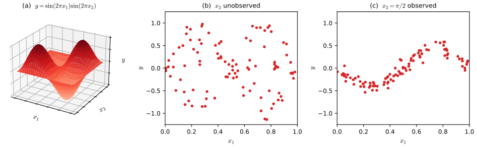
fig_2_1. Download: PDF · SVGThe book's bent coin (Figure 2.2, a photograph, not reproduced) separates two meanings of probability. That it lands concave side up 60% of the time is a frequency of a repeatable event. Whether its concave side is heads is not repeatable at all, just unknown; assigning it probability 0.5 is a Bayesian statement of uncertainty, which can then be updated by data (Section 2.6, Exercise 2.40).
2.1 The rules of probability
See also: Bayesian and Probabilistic Machine Learning, Section 1.2 (the same rules, from the same frequency argument).
2.1.1 A medical screening example
pp. 25–26 One percent of a population has a cancer. A test is positive for 90% of those who have it (so 10% are false negatives) and for 3% of those who do not (false positives). Two questions: how often is a randomly screened person positive, and how likely is cancer after a positive result? Figure 2.3 draws the error rates as two groups of 100 people.
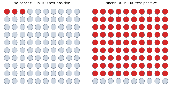
fig_2_3. Download: PDF · SVG2.1.2 The sum and product rules
pp. 26–28 Let \(X\) take values \(x_1,\dots,x_L\) and \(Y\) values \(y_1,\dots,y_M\). In \(N\) trials let \(n_{ij}\) count the outcomes with \(X=x_i,Y=y_j\), and let \(c_i=\sum_jn_{ij}\) and \(r_j=\sum_in_{ij}\) be the column and row totals (Figure 2.4 of the book draws this grid; Figure 2.5 below shows it filled with data). In the limit \(N\to\infty\) the fractions define the probabilities.
Definition 2.1 (joint, marginal and conditional probability; the two rules) (2.1)–(2.9)
\[ p(X=x_i,Y=y_j)=\frac{n_{ij}}{N}, \tag{2.1} \] \[ p(X=x_i)=\frac{c_i}{N},\qquad \sum_{i=1}^{L}p(X=x_i)=1, \tag{2.3} \] \[ p(Y=y_j\given X=x_i)=\frac{n_{ij}}{c_i},\qquad \sum_{j=1}^{M}p(Y=y_j\given X=x_i)=1. \tag{2.6} \](The first parts are (2.2) and (2.5).) Because \(c_i=\sum_jn_{ij}\) and \(n_{ij}/N=(n_{ij}/c_i)(c_i/N)\), these satisfy, in compact notation,
\[ \textbf{sum rule}\qquad p(X)=\sum_Yp(X,Y), \tag{2.8} \] \[ \textbf{product rule}\qquad p(X,Y)=p(Y\given X)\,p(X). \tag{2.9} \]A marginal is obtained by summing out (marginalising) the other variables.
Why only these two rules? The frequency argument presupposes repeatable trials. Cox (1946) showed that any system of real-valued degrees of belief obeying a few consistency requirements must, after a monotone rescaling, obey exactly (2.8) and (2.9); the book returns to this in Section 2.6. Everything else in this chapter, and most of the probabilistic machinery of the book, is derived from these two lines.
2.1.3 Bayes' theorem
pp. 28–29 Writing the product rule both ways, \(p(Y\given X)p(X)=p(X,Y)=p(X\given Y)p(Y)\), and dividing by \(p(X)>0\):
\[ p(Y\given X)=\frac{p(X\given Y)\,p(Y)}{p(X)},\qquad p(X)=\sum_Yp(X\given Y)\,p(Y). \tag{2.10, 2.11} \]The denominator is the normaliser that makes the left side sum to one over \(Y\). Figure 2.5 shows a joint distribution estimated from 60 samples, with its marginals and one conditional.
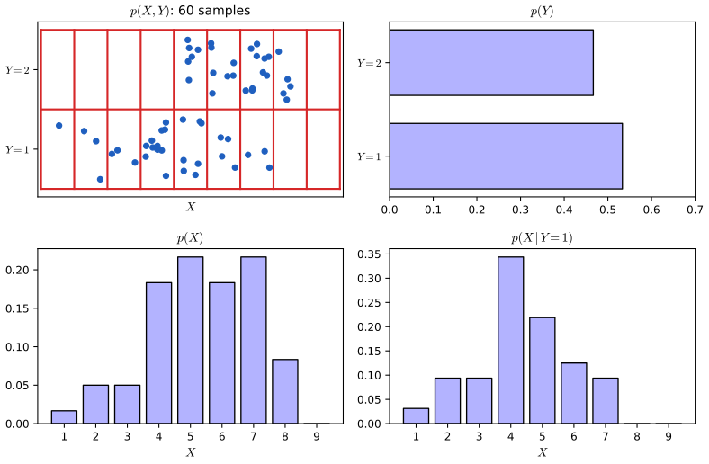
fig_2_5. Download: PDF · SVG2.1.4 Medical screening revisited
pp. 30–31 Let \(C\in\{0,1\}\) be the disease status and \(T\in\{0,1\}\) the test result, with \(p(C=1)=1/100\) (2.12), \(p(C=0)=99/100\) (2.13), and \(p(T=1\given C=1)=90/100\), \(p(T=0\given C=1)=10/100\), \(p(T=1\given C=0)=3/100\), \(p(T=0\given C=0)=97/100\) (2.14)–(2.17), each pair summing to one (2.18), (2.19).
Result 2.1 (screening: the two answers) (2.20)–(2.22)
\[ p(T=1)=\tfrac{3}{100}\cdot\tfrac{99}{100}+\tfrac{90}{100}\cdot\tfrac{1}{100}=\tfrac{387}{10\,000}=0.0387, \tag{2.20} \] \[ p(C=1\given T=1)=\frac{p(T=1\given C=1)\,p(C=1)}{p(T=1)}=\frac{90}{387}\approx0.23. \tag{2.22} \]So \(p(C=0\given T=1)=297/387\approx0.77\). Also \(p(T=0)=0.9613\) and \(p(C=1\given T=0)=10/9613\approx0.001\).
A wording slip. After (2.20) the book says that, since \(p(T=0)=0.9613\), "there is a roughly 96% chance that [they] do not have cancer". The number 0.9613 is the probability of a negative test; the probability of not having cancer is \(p(C=0)=0.99\), and after a negative test it is \(1-10/9613\approx0.999\).
Filling the gap 2.1: Bayes' theorem in odds form, natural frequencies and repeated tests pp. 30–31
Why is the posterior so small, how does it depend on the prevalence, and what happens after a second test? The book calls the result counter-intuitive; the odds form makes it transparent.
Derivation
Odds form. Divide Bayes' theorem for \(C=1\) by the same for \(C=0\); the normaliser \(p(T=1)\) cancels:
\[ \frac{p(C=1\given T=1)}{p(C=0\given T=1)}=\frac{p(T=1\given C=1)}{p(T=1\given C=0)}\cdot\frac{p(C=1)}{p(C=0)} . \]Posterior odds equal the likelihood ratio (here \(0.90/0.03=30\)) times the prior odds (\(1/99\)): \(30/99=90/297\), the odds of 23%. A test multiplies the odds by a fixed factor; when the prior odds are 1:99, even a factor of 30 leaves the odds below 1. With prevalence 0.1% (Exercise 2.1) the prior odds are 1:999 and the posterior odds 30:999, a probability of 2.9%.
Natural frequencies. In 10,000 people, 100 have cancer and 90 of them test positive; 9,900 do not and 297 of them test positive. Of the 387 positives, 90 are ill: \(90/387\). The large healthy group produces most positive tests even though its error rate is small.
Repeated tests. Suppose two test results \(T_1,T_2\) are conditionally independent given \(C\): \(p(T_1,T_2\given C)=p(T_1\given C)p(T_2\given C)\). Then by the product rule and Bayes,
\[ p(C\given T_1,T_2)=\frac{p(T_2\given C)\,p(T_1\given C)\,p(C)}{\sum_{c}p(T_2\given c)\,p(T_1\given c)\,p(c)}=\frac{p(T_2\given C)\,p(C\given T_1)}{\sum_cp(T_2\given c)\,p(c\given T_1)}, \]where the second form divides numerator and denominator by \(p(T_1)\). The posterior after the first test plays the role of the prior for the second, and in odds form the likelihood ratios multiply: two positives give odds \(30^2/99\), a probability of \(0.90\). The assumption matters: a second test that repeats the same systematic error is not independent given \(C\), and the update would be smaller. ∎
2.1.5 Prior and posterior probabilities
p. 31 \(p(C)\) is the prior, the probability before the test is seen; \(p(C\given T)\) is the posterior. The test provides strong evidence (a likelihood ratio of 30), but evidence multiplies the prior odds, it does not replace them; the low prior is why a positive result still leaves only a 23% chance of disease.
2.1.6 Independent variables
p. 31 \(X\) and \(Y\) are independent if \(p(X,Y)=p(X)p(Y)\). By the product rule this is equivalent to \(p(Y\given X)=p(Y)\) wherever \(p(X)>0\), and then Bayes gives \(p(X\given Y)=p(X)\): observing one variable does not change beliefs about the other. A test with \(p(T\given C)=p(T)\), i.e. the same positive rate in both groups, is useless.
2.2 Probability densities
See also: Bayesian and Probabilistic Machine Learning, Section 1.2.1 (densities and the Jacobian factor).
pp. 32–33 For a continuous variable every single value has probability zero, so one uses a density: \(p(x)\,\delta x\) is the probability of \((x,x+\delta x)\) as \(\delta x\to0\), and
\[ p(x\in(a,b))=\int_a^bp(x)\,\d x,\qquad p(x)\ge0,\qquad \int_{-\infty}^{\infty}p(x)\,\d x=1. \tag{2.23–2.25} \]The cumulative distribution function \(P(z)=\int_{-\infty}^{z}p(x)\,\d x\) (2.26) satisfies \(P'(x)=p(x)\) at every point where \(p\) is continuous (fundamental theorem of calculus). Note that a density can exceed 1; only its integrals are probabilities. In \(D\) dimensions \(p(\mathbf{x})\ge0\) and \(\int p(\mathbf{x})\,\d\mathbf{x}=1\) (2.27), (2.28).
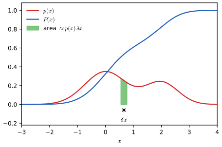
fig_2_6. Download: PDF · SVGFor two real variables the rules read
\[ p(x)=\int p(x,y)\,\d y,\qquad p(x,y)=p(y\given x)\,p(x), \tag{2.29, 2.30} \] \[ p(y\given x)=\frac{p(x\given y)\,p(y)}{p(x)},\qquad p(x)=\int p(x\given y)\,p(y)\,\d y. \tag{2.31, 2.32} \]Filling the gap 2.2: why the sum and product rules hold for densities p. 33
The book justifies (2.29)–(2.32) informally, by binning and letting the bin width go to zero, and says a formal treatment needs measure theory. Both arguments fit in a few lines.
Derivation
The binning heuristic, made explicit. Cut both axes into bins of width \(\Delta\) with centres \(x_i,y_j\). If \(p(x,y)\) is continuous, the probability of cell \((i,j)\) is \(P_{ij}=p(x_i,y_j)\Delta^2+o(\Delta^2)\). The discrete sum rule gives \(P_i=\sum_jP_{ij}=\Delta\big[\sum_jp(x_i,y_j)\Delta\big]+o(\Delta)\); the bracket is a Riemann sum converging to \(\int p(x_i,y)\,\d y\), so the density of \(x\) at \(x_i\), \(\lim P_i/\Delta\), is (2.29). Likewise \(P_{ij}/P_i\to p(x_i,y_j)\Delta/p(x_i)\), so the conditional density is \(p(x,y)/p(x)\), which is (2.30).
The rigorous version. Let \((x,y)\) have a joint density, meaning \(P((x,y)\in A)=\iint_Ap(x,y)\,\d x\,\d y\) for every (measurable) set \(A\). For a set \(B\) of \(x\)-values, take \(A=B\times\R\); since \(p\ge0\), Tonelli's theorem lets us integrate over \(y\) first:
\[ P(x\in B)=\int_B\Big[\int p(x,y)\,\d y\Big]\d x , \]so the bracket is a density of \(x\): that is (2.29). Define \(p(y\given x)=p(x,y)/p(x)\) where \(p(x)>0\). For each such \(x\) it is non-negative and integrates to \(p(x)/p(x)=1\) over \(y\), so it is a density in \(y\); and (2.30) holds by construction (where \(p(x)=0\), (2.29) forces \(p(x,y)=0\) for almost every \(y\), so (2.30) holds whatever value is given to \(p(y\given x)\)). Exchanging the roles of \(x\) and \(y\) gives \(p(x,y)=p(x\given y)p(y)\); equating the two and dividing by \(p(x)>0\) gives Bayes (2.31), and integrating \(p(x,y)=p(x\given y)p(y)\) over \(y\) gives (2.32). The same steps work with sums in place of integrals for any discrete variable, which covers mixed cases such as \(p(\mathcal{C}_k\given\mathbf{x})=p(\mathbf{x}\given\mathcal{C}_k)p(\mathcal{C}_k)/\sum_jp(\mathbf{x}\given\mathcal{C}_j)p(\mathcal{C}_j)\), the form used for classification throughout the book. ∎
2.2.1 Example distributions
pp. 33–34 A constant density on the whole line cannot be normalised (it is improper); restricted to \((c,d)\) it is the uniform density \(p(x)=1/(d-c)\) (2.33). The exponential and Laplace densities are
\[ p(x\given\lambda)=\lambda e^{-\lambda x}\ (x\ge0),\qquad p(x\given\mu,\gamma)=\frac{1}{2\gamma}\exp\Big(-\frac{|x-\mu|}{\gamma}\Big). \tag{2.34, 2.35} \]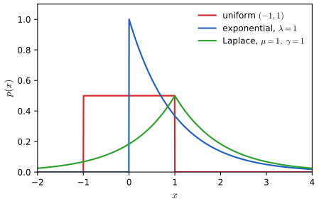
fig_2_7. Download: PDF · SVGThe Dirac delta \(\delta(x-\mu)\) (2.36) is the limit of ever narrower unit-area spikes at \(\mu\); its defining property is \(\int f(x)\delta(x-\mu)\,\d x=f(\mu)\) for continuous \(f\). The empirical distribution of a data set \(\D=\{x_1,\dots,x_N\}\) puts mass \(1/N\) on each point:
\[ p(x\given\D)=\frac1N\sum_{n=1}^{N}\delta(x-x_n). \tag{2.37} \]2.2.2 Expectations and covariances
See also: Bayesian and Probabilistic Machine Learning, Section 1.2.2 and its Result 1.3 (variance and covariance identities).
pp. 34–36 The expectation of \(f\) is \(\E[f]=\sum_xp(x)f(x)\) or \(\int p(x)f(x)\,\d x\) (2.38), (2.39), and with samples \(x_1,\dots,x_N\) from \(p\)
\[ \E[f]\simeq\frac1N\sum_{n=1}^{N}f(x_n). \tag{2.40} \]A subscript names the variable averaged over, \(\E_x[f(x,y)]\) (2.41) being a function of \(y\); the conditional expectation is \(\E_x[f\given y]=\int p(x\given y)f(x)\,\d x\) (2.42), (2.43). The variance and covariance are
\[ \var[f]=\E\big[(f(x)-\E[f(x)])^2\big]=\E[f(x)^2]-\E[f(x)]^2, \tag{2.44, 2.45} \] \[ \cov[x,y]=\E_{x,y}\big[\{x-\E[x]\}\{y-\E[y]\}\big]=\E_{x,y}[xy]-\E[x]\E[y], \tag{2.47} \] \[ \cov[\mathbf{x},\mathbf{y}]=\E_{\mathbf{x},\mathbf{y}}\big[\{\mathbf{x}-\E[\mathbf{x}]\}\{\mathbf{y}^\T-\E[\mathbf{y}^\T]\}\big]=\E_{\mathbf{x},\mathbf{y}}[\mathbf{x}\mathbf{y}^\T]-\E[\mathbf{x}]\E[\mathbf{y}^\T], \tag{2.48} \]with \(\cov[\mathbf{x}]\equiv\cov[\mathbf{x},\mathbf{x}]\); (2.46) is (2.45) for \(f(x)=x\).
Filling the gap 2.3: the delta function, and why the sample average (2.40) works pp. 34–35
The book says (2.37) integrates to one, that (2.40) follows from it, and that (2.40) "becomes exact in the limit". Here is what each of these means and how fast the limit is approached.
Derivation
The empirical distribution (Exercises 2.6, 2.7). By the sifting property with \(f\equiv1\), \(\int\delta(x-x_n)\,\d x=1\), so \(\int p(x\given\D)\,\d x=\frac1N\sum_n1=1\); and \(\int f(x)p(x\given\D)\,\d x=\frac1N\sum_nf(x_n)\). So (2.40) is the exact expectation under the empirical distribution; it approximates \(\E_p[f]\) because the empirical distribution approximates \(p\) when the \(x_n\) are drawn from \(p\).
Unbiasedness and the error. Let \(\hat f_N=\frac1N\sum_nf(x_n)\) with \(x_n\) independent draws from \(p\) and \(\var[f]\lt \infty\). By linearity \(\E[\hat f_N]=\E[f]\): the estimate is unbiased. By independence the covariances of different terms vanish (gap 2.4), so
\[ \var[\hat f_N]=\frac{1}{N^2}\sum_{n=1}^{N}\var[f(x_n)]=\frac{\var[f]}{N}. \]The typical error is \(\sqrt{\var[f]/N}\), independent of the dimension of \(x\), which is why sampling-based estimates are used for the very high-dimensional expectations of later chapters.
The limit. Chebyshev's inequality, \(P(|z-\E z|\ge\varepsilon)\le\var[z]/\varepsilon^2\), applied to \(z=\hat f_N\) gives \(P(|\hat f_N-\E[f]|\ge\varepsilon)\le\var[f]/(N\varepsilon^2)\to0\) for every \(\varepsilon>0\) (the weak law of large numbers). The strong law (which needs only \(\E|f|\lt \infty\)) says that \(\hat f_N\to\E[f]\) with probability one; this is the precise sense in which (2.40) "becomes exact". ∎
Filling the gap 2.4: covariance identities, independence and correlation pp. 35–36, Exercises 2.8–2.11, 2.39
The book states that independent variables have zero covariance. The converse is false, and the covariance matrix has properties used constantly later.
Derivation
(2.45) and (2.47). Write \(m=\E[f]\). Expanding, \(\E[(f-m)^2]=\E[f^2]-2m\E[f]+m^2=\E[f^2]-m^2\). The same expansion with two factors gives (2.47), and with outer products (2.48).
Independence implies zero covariance. If \(p(x,y)=p(x)p(y)\) then \(\E[xy]=\iint xy\,p(x)p(y)\,\d x\,\d y=\E[x]\E[y]\) (the double integral factorises), so \(\cov[x,y]=0\). Consequently \(\var[x+z]=\var[x]+\var[z]+2\cov[x,z]=\var[x]+\var[z]\) for independent \(x,z\) (Exercise 2.10), and the variance of a sum of \(N\) independent terms is the sum of the variances, used in gap 2.3.
The converse fails (Exercise 2.39). Let \(y_1\) be symmetric about 0 with \(\E[y_1^4]\lt \infty\) and \(y_2=y_1^2\). Then \(p(y_2\given y_1)=\delta(y_2-y_1^2)\) depends on \(y_1\), but \(\cov[y_1,y_2]=\E[y_1^3]-\E[y_1]\E[y_1^2]=0-0=0\), because odd moments of a symmetric variable vanish. Covariance measures only linear dependence; mutual information (Section 2.5.7) detects any dependence.
Covariance matrices are positive semidefinite. For any fixed vector \(\mathbf{a}\), \(\mathbf{a}^\T\cov[\mathbf{x}]\mathbf{a}=\E[(\mathbf{a}^\T(\mathbf{x}-\E\mathbf{x}))^2]=\var[\mathbf{a}^\T\mathbf{x}]\ge0\), with equality only if \(\mathbf{a}^\T\mathbf{x}\) is almost surely constant. It is also symmetric, and \(\cov[\mathbf{A}\mathbf{x}+\mathbf{b}]=\mathbf{A}\cov[\mathbf{x}]\mathbf{A}^\T\) by linearity. ∎
2.3 The Gaussian distribution
See also: Bayesian and Probabilistic Machine Learning, Section 1.2.4 (the same results with full proofs) and its Section 2.3 (the multivariate Gaussian).
pp. 36–37 The univariate Gaussian with mean \(\mu\) and variance \(\sigma^2\) (precision \(\beta=1/\sigma^2\)) is
\[ \N(x\given\mu,\sigma^2)=\frac{1}{(2\pi\sigma^2)^{1/2}}\exp\Big\{-\frac{1}{2\sigma^2}(x-\mu)^2\Big\}. \tag{2.49} \]It is positive (2.50) and integrates to one (2.51); its special status comes from maximum entropy (Section 2.5.4) and the central limit theorem (Section 3.2 of the book).
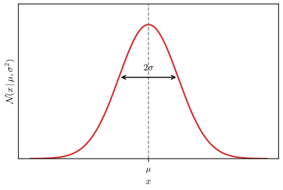
fig_2_8. Download: PDF · SVG2.3.1 Mean and variance
Result 2.2 (the Gaussian is normalised; its moments and mode) (2.51)–(2.54), Exercises 2.12–2.14
\[ \int_{-\infty}^{\infty}\N(x\given\mu,\sigma^2)\,x\,\d x=\mu,\qquad \int_{-\infty}^{\infty}\N(x\given\mu,\sigma^2)\,x^2\,\d x=\mu^2+\sigma^2, \tag{2.52, 2.53} \]so \(\var[x]=\sigma^2\) (2.54), and the mode (maximum) is at \(x=\mu\).
Proof sketch (full proofs: companion course, Results 1.4 and 1.5)
Normalisation. With \(I=\int e^{-x^2/2\sigma^2}\d x\), \(I^2=\iint e^{-(x^2+y^2)/2\sigma^2}\d x\,\d y\). In polar coordinates (\(\d x\,\d y=r\,\d r\,\d\theta\), the Jacobian of Result 2.7) and with \(u=r^2\), \(I^2=2\pi\int_0^\infty e^{-u/2\sigma^2}\tfrac12\d u=2\pi\sigma^2\). Shifting by \(\mu\) does not change the integral.
Moments. With \(z=x-\mu\), \(\E[x]=\mu+\int z\N(z\given0,\sigma^2)\d z=\mu\) because the integrand is odd. Differentiating the identity \(\int e^{-(x-\mu)^2/2\sigma^2}\d x=(2\pi\sigma^2)^{1/2}\) with respect to \(\sigma^2\) gives \(\int\frac{(x-\mu)^2}{2\sigma^4}e^{-(x-\mu)^2/2\sigma^2}\d x=\frac12(2\pi)^{1/2}\sigma^{-1}\), i.e. \(\E[(x-\mu)^2]=\sigma^2\), hence \(\E[x^2]=\sigma^2+\mu^2\).
Mode. \(\frac{\d}{\d x}\N=-\frac{x-\mu}{\sigma^2}\N\), which vanishes only at \(\mu\) and changes sign from \(+\) to \(-\) there. Details: Result 1.4 and Result 1.5 of the companion course. ∎
2.3.2 Likelihood function
pp. 37–39 Let \(\mathsf{x}=(x_1,\dots,x_N)\) be i.i.d. (independent, identically distributed) draws from a Gaussian with unknown \(\mu,\sigma^2\). Density estimation from finitely many points is ill-posed (any density positive at the data is a candidate); restricting to Gaussians makes it well posed. By independence the probability of the data is a product, which, as a function of the parameters, is the likelihood:
\[ p(\mathsf{x}\given\mu,\sigma^2)=\prod_{n=1}^{N}\N(x_n\given\mu,\sigma^2), \tag{2.55} \] \[ \ln p(\mathsf{x}\given\mu,\sigma^2)=-\frac{1}{2\sigma^2}\sum_{n=1}^{N}(x_n-\mu)^2-\frac N2\ln\sigma^2-\frac N2\ln(2\pi). \tag{2.56} \]Logs turn the product into a sum, which avoids numerical underflow, and do not move the maximiser because \(\ln\) is increasing.
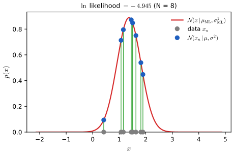
fig_2_9. Download: PDF · SVGResult 2.3 (maximum likelihood for the Gaussian) (2.57), (2.58), Exercise 2.15
If at least two of the \(x_n\) differ, (2.56) has a unique global maximum at
\[ \mu\ML=\frac1N\sum_{n=1}^{N}x_n,\qquad \sigma^2\ML=\frac1N\sum_{n=1}^{N}(x_n-\mu\ML)^2. \tag{2.57, 2.58} \]If all \(x_n\) are equal, the likelihood is unbounded as \(\sigma^2\to0\) and has no maximum.
Filling the gap 2.5: the stationary point is the global maximum, and why \(\mu\) decouples pp. 38–39
The book sets derivatives to zero. That finds stationary points; it does not show that the one found is the maximum, nor what happens at the boundary \(\sigma^2\to0\).
Derivation
Write \(\ell(\mu,v)\) for (2.56) with \(v=\sigma^2>0\) and \(\bar x=\mu\ML\), \(s=\frac1N\sum(x_n-\bar x)^2\).
Step 1: \(\mu\) for fixed \(v\). The decomposition \(\sum_n(x_n-\mu)^2=\sum_n(x_n-\bar x)^2+N(\bar x-\mu)^2\) holds because the cross term \(2(\bar x-\mu)\sum_n(x_n-\bar x)\) is zero. So \(\ell(\mu,v)=\ell(\bar x,v)-\frac{N}{2v}(\bar x-\mu)^2\le\ell(\bar x,v)\), with equality only at \(\mu=\bar x\), whatever \(v\) is. This is the decoupling the book mentions: the best \(\mu\) does not depend on \(v\).
Step 2: the profile in \(v\). \(\ell(\bar x,v)=-\frac{Ns}{2v}-\frac N2\ln v+\const\), with derivative \(\frac{N}{2v^2}(s-v)\): positive for \(v\lt s\), negative for \(v>s\). If \(s>0\) the profile increases up to \(v=s\) and decreases afterwards, so \(v=s\) is its unique global maximiser. Combining the two steps, \(\ell(\mu,v)\le\ell(\bar x,v)\le\ell(\bar x,s)\) for all \((\mu,v)\), with equality only at \((\bar x,s)\).
The degenerate case. If all points coincide, \(s=0\) and \(\ell(\bar x,v)=-\frac N2\ln v+\const\to+\infty\) as \(v\to0\). The same collapse of a Gaussian onto a data point is the singularity of maximum likelihood for mixtures (Chapter 15 of the book). ∎
2.3.3 Bias of maximum likelihood
See also: Bayesian and Probabilistic Machine Learning, Result 1.8 (the same bias, Exercises 1.12 and 1.13 there).
Result 2.4 (bias of the maximum likelihood variance) (2.59)–(2.63), Exercises 2.16, 2.17
Over data sets of \(N\) i.i.d. draws from \(\N(\mu,\sigma^2)\),
\[ \E[\mu\ML]=\mu,\qquad \E[\sigma^2\ML]=\Big(\frac{N-1}{N}\Big)\sigma^2, \tag{2.59, 2.60} \]while \(\hat\sigma^2=\frac1N\sum_n(x_n-\mu)^2\) (2.61), which uses the true mean, has \(\E[\hat\sigma^2]=\sigma^2\) (2.62), and \(\widetilde\sigma^2=\frac{1}{N-1}\sum_n(x_n-\mu\ML)^2\) (2.63) is unbiased.
Filling the gap 2.6: where the factor \((N-1)/N\) comes from, the exact distribution, and why bias is not the whole story pp. 39–40
The book gives the result as "straightforward to show" and an intuition through Figure 2.10. One identity proves it; two more facts show what the bias does and does not mean.
Derivation
The proof. Use the decomposition of gap 2.5 with the true mean: \(\sum_n(x_n-\mu)^2=N\sigma^2\ML+N(\mu\ML-\mu)^2\). Take expectations. The left side is \(N\sigma^2\) (each term has expectation \(\sigma^2\); this is (2.62)). On the right, \(\E[\mu\ML]=\mu\) by linearity (2.59) and \(\var[\mu\ML]=\sigma^2/N\) (gap 2.3), so \(\E[N(\mu\ML-\mu)^2]=\sigma^2\). Hence \(N\E[\sigma^2\ML]=N\sigma^2-\sigma^2\), which is (2.60), and multiplying by \(N/(N-1)\) gives (2.63). The book's route through \(\E[x_nx_m]=\mu^2+I_{nm}\sigma^2\) (2.128) is worked in Exercise 2.16.
Intuition, made exact. The sample mean is the point that minimises \(\sum_n(x_n-c)^2\) over \(c\), so measuring spread about it gives a smaller sum than measuring about the true mean; the deficit is exactly \(N(\mu\ML-\mu)^2\), whose expectation is one \(\sigma^2\): one "degree of freedom" is used up in estimating \(\mu\).
The exact distribution. For Gaussian data, \(N\sigma^2\ML/\sigma^2\) has a \(\chi^2\) distribution with \(N-1\) degrees of freedom and is independent of \(\mu\ML\) (Cochran's theorem: rotate the data vector by an orthogonal matrix whose first row is \((1,\dots,1)/\sqrt N\); the first coordinate becomes \(\sqrt N\mu\ML\) and the other \(N-1\) are independent \(\N(0,\sigma^2)\) variables whose squares add up to \(N\sigma^2\ML\)). So \(\var[\sigma^2\ML]=2(N-1)\sigma^4/N^2\).
Bias is not everything. The mean squared error of an estimator is variance plus squared bias. For \(\sigma^2\ML\) it is \(\frac{2(N-1)}{N^2}\sigma^4+\frac{1}{N^2}\sigma^4=\frac{2N-1}{N^2}\sigma^4\); for the unbiased \(\widetilde\sigma^2=\frac{N}{N-1}\sigma^2\ML\) it is \(\frac{2}{N-1}\sigma^4\). Since \((2N-1)(N-1)\lt 2N^2\), the biased maximum likelihood estimate is the more accurate of the two for every \(N\ge2\). The bias matters in the book's argument not as an inaccuracy in itself but as a symptom: fitting and evaluating on the same data flatters the fit, the mechanism behind over-fitting. ∎
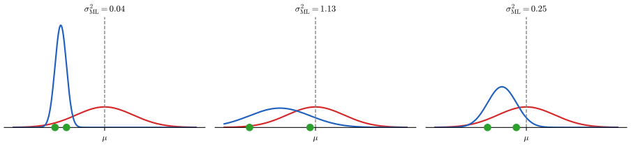
fig_2_10. Download: PDF · SVGThe bias becomes negligible as \(N\) grows, but the same mechanism, much stronger, affects models with many parameters (Section 2.6.3).
2.3.4 Linear regression
See also: Bayesian and Probabilistic Machine Learning, Section 1.2.5 and its Result 1.9 (least squares is maximum likelihood).
pp. 40–42 For the regression problem of Section 1.2 of the book (training inputs \(\mathsf{x}\), targets \(\mathsf{t}\), polynomial \(y(x,\mathbf{w})\)), model the target given the input as Gaussian around the curve:
\[ p(t\given x,\mathbf{w},\sigma^2)=\N\big(t\given y(x,\mathbf{w}),\sigma^2\big), \tag{2.64} \] \[ \ln p(\mathsf{t}\given\mathsf{x},\mathbf{w},\sigma^2)=-\frac{1}{2\sigma^2}\sum_{n=1}^{N}\{y(x_n,\mathbf{w})-t_n\}^2-\frac N2\ln\sigma^2-\frac N2\ln(2\pi). \tag{2.66} \](The likelihood itself is the product (2.65).)
Result 2.5 (least squares is Gaussian maximum likelihood) (2.67)–(2.69), Exercise 2.18
For any fixed \(\sigma^2\), maximising (2.66) over \(\mathbf{w}\) is the same as minimising
\[ E(\mathbf{w})=\frac12\sum_{n=1}^{N}\{y(x_n,\mathbf{w})-t_n\}^2, \tag{2.67} \]so \(\mathbf{w}\ML\) does not depend on \(\sigma^2\); then \(\sigma^2\ML=\frac1N\sum_n\{y(x_n,\mathbf{w}\ML)-t_n\}^2\) (2.68), provided the fit is not exact. The predictive distribution is \(\N(t\given y(x,\mathbf{w}\ML),\sigma^2\ML)\) (2.69).
Proof
(2.66) equals \(-E(\mathbf{w})/\sigma^2-\frac N2\ln\sigma^2+\const\). For fixed \(\sigma^2>0\) the first term is a negative multiple of \(E\), so the maximisers in \(\mathbf{w}\) are the minimisers of \(E\), the same set for every \(\sigma^2\). Substituting, the profile \(-E(\mathbf{w}\ML)/v-\frac N2\ln v\) is maximised exactly as in Step 2 of gap 2.5, at \(v=2E(\mathbf{w}\ML)/N\), which is (2.68); if \(E(\mathbf{w}\ML)=0\) (interpolation) it is unbounded. For a polynomial, \(y=\bm\phi(x)^\T\mathbf{w}\) is linear in \(\mathbf{w}\), and \(\mathbf{w}\ML\) solves the normal equations \(\bm\Phi^\T\bm\Phi\,\mathbf{w}=\bm\Phi^\T\mathsf{t}\) (companion course, Result 1.1). The code checks the equivalence against a direct numerical maximisation of (2.66). ∎
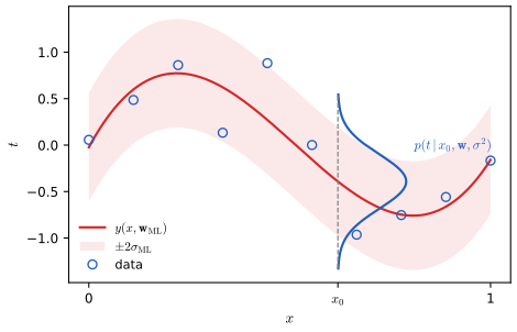
fig_2_11. Download: PDF · SVGThe sum-of-squares error is therefore not an arbitrary choice: it is the negative log likelihood under Gaussian noise. Other noise models give other error functions (for example Laplace noise gives the sum of absolute errors), a pattern used for every loss function in later chapters.
2.4 Transformation of densities
See also: Bayesian and Probabilistic Machine Learning, Filling the gap 1.2 (the Jacobian factor and the moving mode, PRML Exercise 1.4) and the coupling-flow demo there.
pp. 42–45 Under a change of variables \(x=g(y)\) a function simply composes, \(\tilde f(y)=f(g(y))\) (2.70), but a density must also account for how lengths are stretched, because probability, not density, is what is conserved.
Result 2.6 (change of variables in one dimension) (2.71)
Let \(x\) have density \(p_x\) and let \(x=g(y)\) with \(g\) differentiable and strictly monotone, \(g'(y)\neq0\). Then \(y=g^{-1}(x)\) has density
\[ p_y(y)=p_x(x)\left|\frac{\d x}{\d y}\right|=p_x(g(y))\,|g'(y)|. \tag{2.71} \]Filling the gap 2.7: a proof of (2.71), non-monotone maps, and making any density from any other (Exercise 2.19) pp. 42–43
The book argues with \(p_x\delta x\simeq p_y\delta y\). The cumulative distribution function turns this into a proof and shows where the absolute value comes from.
Derivation
Increasing \(g\). \(y\le y_0\iff g(y)\le g(y_0)\iff x\le g(y_0)\), so \(P_y(y_0)=P_x(g(y_0))\). Differentiating with the chain rule gives \(p_y(y_0)=p_x(g(y_0))\,g'(y_0)\), and \(g'>0\).
Decreasing \(g\). Now \(y\le y_0\iff x\ge g(y_0)\), so \(P_y(y_0)=1-P_x(g(y_0))\) and \(p_y(y_0)=-p_x(g(y_0))\,g'(y_0)=p_x(g(y_0))|g'(y_0)|\). The modulus covers both cases.
Non-monotone maps. If \(y=h(x)\) with \(h\) piecewise monotone, split the \(x\)-line into intervals where \(h\) is monotone and apply the above on each; the contributions add:
\[ p_y(y)=\sum_{x:\,h(x)=y}\frac{p_x(x)}{|h'(x)|}. \]For example \(y=x^2\) with \(x\sim\N(0,1)\) gives \(p_y(y)=2\cdot\frac{e^{-y/2}}{\sqrt{2\pi}}\cdot\frac{1}{2\sqrt y}\), the \(\chi^2_1\) density.
Any density from any other (Exercise 2.19). Let \(q\) be a density that is positive on \(\R\) with CDF \(Q\), and \(p\) a target density with CDF \(P\), positive on an interval \(J\) so that \(P:J\to(0,1)\) is a strictly increasing bijection. Put \(y=f(x)=P^{-1}(Q(x))\). Then \(f\) is strictly increasing and \(P(f(x))=Q(x)\); differentiating, \(p(f(x))f'(x)=q(x)\), which is the differential equation asked for, and by the increasing case above \(y\) has density \(q(f^{-1}(y))/f'(f^{-1}(y))=p(y)\). Strict monotonicity matters: where \(f'=0\) on an interval, all of that interval's mass would land on one point and \(p_y\) would contain a delta spike, which is why the book's condition \(0\le f'\) should read \(f'>0\). This is how samplers turn uniform or Gaussian random numbers into other distributions (Chapter 14 of the book), and it is the one-dimensional case of a normalizing flow. ∎
The mode is not invariant. For a function, if \(f'(\hat x)=0\) then \(\tilde f'(\hat y)=f'(g(\hat y))g'(\hat y)=0\) (2.72) at \(\hat x=g(\hat y)\): maxima map to maxima. For a density, write \(g'=s|g'|\) with \(s=\pm1\); differentiating \(p_y=p_x(g)\,s\,g'\) gives
\[ p_y'(y)=s\,p_x'(g(y))\{g'(y)\}^2+s\,p_x(g(y))\,g''(y). \tag{2.73} \]The second term spoils the correspondence unless \(g''=0\), i.e. unless \(g\) is linear. The book's example takes \(p_x=\N(6,1)\) and the logistic change of variables
\[ x=g(y)=\ln y-\ln(1-y)+5,\qquad y=g^{-1}(x)=\frac{1}{1+\exp(-x+5)}. \tag{2.74, 2.75} \]Filling the gap 2.8: where exactly the mode of \(p_y\) goes pp. 43–44, Figure 2.12
The book shows numerically that the mode moves. For a Gaussian \(p_x\) and a logistic map the new mode solves a simple equation, which gives the exact value, explains the direction of the shift, and says when the mode is unique.
Derivation
Take \(p_x=\N(\mu,\sigma^2)\) and the slightly more general \(g(y)=c+a^{-1}\ln\frac{y}{1-y}\) with \(a>0\) (the book has \(a=1,c=5\)), so \(y=\sigma_{\rm log}(a(x-c))\), the logistic sigmoid. Then \(g'(y)=\frac{1}{a\,y(1-y)}>0\) and \(g''(y)=-\frac{1-2y}{a\,y^2(1-y)^2}\), so \(g''/g'^2=a(2y-1)\).
Because \(p_y>0\) on \((0,1)\), its maxima are those of \(\ln p_y=\ln p_x(g(y))+\ln g'(y)\). The derivative is \(g'\,[\,(\ln p_x)'(g)+g''/g'^2\,]\) (this is (2.73) divided by \(p_y\)), and \(g'>0\), so the stationarity condition is \((\ln p_x)'(x)+a(2y-1)=0\) at \(x=g(y)\). For the Gaussian \((\ln p_x)'(x)=-(x-\mu)/\sigma^2\), hence
\[ \frac{x-\mu}{\sigma^2}=a\,(2y-1),\qquad y=\sigma_{\rm log}(a(x-c)). \]Uniqueness. The function \(h(x)=(x-\mu)/\sigma^2-a(2\sigma_{\rm log}(a(x-c))-1)\) has \(h'(x)=1/\sigma^2-2a^2\sigma_{\rm log}'\ge1/\sigma^2-a^2/2\), using \(\sigma_{\rm log}'\le\frac14\). If \(a\sigma\lt \sqrt2\), \(h\) is strictly increasing and goes from \(-\infty\) to \(+\infty\), so it has exactly one root; since \(p_y\to0\) at both ends of \((0,1)\), that root is the maximum. (For larger \(a\sigma\), \(p_y\) can be bimodal, with peaks pushed towards 0 and 1.)
The book's numbers. With \(\mu=6,\sigma=1,a=1,c=5\): \(x-6=2\sigma_{\rm log}(x-5)-1\), whose root is \(x=6.688\), i.e. \(\hat y=0.844\). The naive answer, \(g^{-1}(\hat x)=\sigma_{\rm log}(1)=0.731\), is the mode of the green curve \(p_x(g(y))\). Since \(\mu>c\) puts most mass where \(y>\frac12\), the Jacobian factor \(1/(y(1-y))\) grows towards \(y=1\) and drags the mode up. ∎
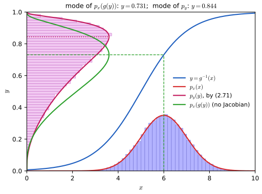
fig_2_12. Download: PDF · SVG2.4.1 Multivariate distributions
pp. 44–45 For \(\mathbf{x}=\mathbf{g}(\mathbf{y})\) with \(\mathbf{x},\mathbf{y}\in\R^D\):
Result 2.7 (change of variables in \(D\) dimensions) (2.76), (2.77)
If \(\mathbf{g}\) is a continuously differentiable bijection with a continuously differentiable inverse (a diffeomorphism), then
\[ p_{\mathbf{y}}(\mathbf{y})=p_{\mathbf{x}}(\mathbf{g}(\mathbf{y}))\,|\det\mathbf{J}(\mathbf{y})|,\qquad J_{ij}=\frac{\partial g_i}{\partial y_j}. \tag{2.76, 2.77} \]Equivalently, with the forward map \(\mathbf{y}=\mathbf{f}(\mathbf{x})=\mathbf{g}^{-1}(\mathbf{x})\), \(p_{\mathbf{y}}(\mathbf{y})=p_{\mathbf{x}}(\mathbf{x})\,/\,|\det(\partial\mathbf{f}/\partial\mathbf{x})|\).
Filling the gap 2.9: why a determinant, the inverse form, and the example (2.78)–(2.79) pp. 44–45, Exercise 2.20
The book explains the determinant as a ratio of volumes. Here is the argument, the identity that converts between the two forms of the formula, and the full analysis of the book's two-dimensional example, including that it is invertible at all.
Derivation
Proof of (2.76). For any (measurable) set \(B\) of \(\mathbf{y}\)-values, \(\mathbf{y}\in B\iff\mathbf{x}\in\mathbf{g}(B)\). The change-of-variables theorem for multiple integrals (valid for diffeomorphisms) gives
\[ P(\mathbf{y}\in B)=\int_{\mathbf{g}(B)}p_{\mathbf{x}}(\mathbf{x})\,\d\mathbf{x}=\int_Bp_{\mathbf{x}}(\mathbf{g}(\mathbf{y}))\,|\det\mathbf{J}(\mathbf{y})|\,\d\mathbf{y}. \]Since this holds for every \(B\), the integrand is the density of \(\mathbf{y}\).
Why the determinant is a volume ratio. To first order, \(\mathbf{g}(\mathbf{y}+\bm\epsilon)\approx\mathbf{g}(\mathbf{y})+\mathbf{J}\bm\epsilon\). A small cube with edges \(h\mathbf{e}_1,\dots,h\mathbf{e}_D\) at \(\mathbf{y}\) is mapped approximately to the parallelepiped with edges \(h\mathbf{J}\mathbf{e}_j\), the columns of \(h\mathbf{J}\), whose volume is \(|\det\mathbf{J}|h^D\). Probability is conserved, so density times volume is the same on both sides: \(p_{\mathbf{y}}h^D=p_{\mathbf{x}}|\det\mathbf{J}|h^D\). The absolute value is there because orientation (the sign of the determinant) does not affect volume. (The book's text then says the volume element around \(\mathbf{x}\) maps to one "around the point \(\mathbf{y}=\mathbf{g}(\mathbf{x})\)" and that "(2.77) follows": with its own convention \(\mathbf{x}=\mathbf{g}(\mathbf{y})\) the point is \(\mathbf{y}=\mathbf{g}^{-1}(\mathbf{x})\), and the formula meant is (2.76).)
The inverse form. Differentiating \(\mathbf{f}(\mathbf{g}(\mathbf{y}))=\mathbf{y}\) with the chain rule gives \(\frac{\partial\mathbf{f}}{\partial\mathbf{x}}\,\mathbf{J}=\mathbf{I}\), so the two Jacobians are inverse matrices and \(|\det\mathbf{J}|=1/|\det(\partial\mathbf{f}/\partial\mathbf{x})|\). Normalizing flows (Chapter 18 of the book) are specified by the forward map, so they use this form, and they choose architectures whose Jacobian determinant is cheap, for example triangular.
The example. The book's map is given forward, \(\mathbf{y}=\mathbf{f}(\mathbf{x})\):
\[ y_1=x_1+\tanh(5x_1),\qquad y_2=x_2+\tanh(5x_2)+\frac{x_1^3}{3}. \tag{2.78, 2.79} \]Its Jacobian (Exercise 2.20) is lower triangular:
\[ \frac{\partial\mathbf{y}}{\partial\mathbf{x}}=\begin{pmatrix}1+5\sech^2(5x_1)&0\\ x_1^2&1+5\sech^2(5x_2)\end{pmatrix},\qquad \det=\big(1+5\sech^2(5x_1)\big)\big(1+5\sech^2(5x_2)\big)\ge1. \]Invertibility. Let \(\phi(u)=u+\tanh(5u)\). Then \(\phi'(u)=1+5\sech^2(5u)\ge1\), so \(\phi\) is strictly increasing with \(\phi(u)\to\pm\infty\) as \(u\to\pm\infty\): a bijection of \(\R\). Hence \(x_1=\phi^{-1}(y_1)\), then \(x_2=\phi^{-1}(y_2-x_1^3/3)\): every \(\mathbf{y}\) has exactly one preimage, and the inverse is smooth by the inverse function theorem (\(\phi'\ge1\)). The transformed density is therefore
\[ p_{\mathbf{y}}(\mathbf{y})=\frac{p_{\mathbf{x}}(\mathbf{x})}{\big(1+5\sech^2(5x_1)\big)\big(1+5\sech^2(5x_2)\big)},\qquad \mathbf{x}=\mathbf{f}^{-1}(\mathbf{y}). \]The stretching factor is up to 6 near the axes \(x_i=0\) and close to 1 away from them, so a Gaussian blob centred at the origin is thinned out along the axes and its mass concentrates in four lobes (Figure 2.13). The shear \(x_1^3/3\) bends the picture but, sitting below the diagonal, does not change the determinant. The code computes the inverse by Newton's method, checks the Jacobian against automatic differentiation and checks that the transformed density integrates to one. ∎
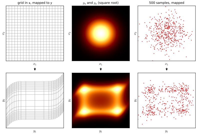
fig_2_13. Download: PDF · SVG2.5 Information theory
See also: Bayesian and Probabilistic Machine Learning, Section 1.6 (entropy, maximum entropy, KL and mutual information, with Results 1.20 to 1.23) and the toolkit (Jensen's inequality, KL, Lagrange multipliers).
2.5.1 Entropy
pp. 46–47 The information gained by observing an outcome \(x\) should depend only on its probability, be larger for less probable outcomes, and add up for independent outcomes. The book states that these requirements force a logarithm:
\[ h(x)=-\log_2p(x),\qquad \H[x]=-\sum_xp(x)\log_2p(x), \tag{2.80, 2.81} \]with \(0\log0=0\) (the limit of \(\epsilon\ln\epsilon\)). The entropy \(\H\) is the average information. A uniform variable on 8 states has \(\H=3\) bits; the distribution \((\frac12,\frac14,\frac18,\frac1{16},\frac1{64},\frac1{64},\frac1{64},\frac1{64})\) has \(\H=2\) bits, and the prefix code 0, 10, 110, 1110, 111100, 111101, 111110, 111111 has average length exactly 2 bits (Cover and Thomas, 1991). From here on logarithms are natural and the unit is the nat (1 nat \(=1/\ln2\) bits).
Filling the gap 2.10: why the logarithm (Exercise 2.21) p. 46
"It is easily shown that \(h\) must be given by the logarithm." The proof is the solution of Cauchy's functional equation; it needs monotonicity (or continuity), which the book assumes but does not use explicitly.
Derivation
Claim. Let \(h:(0,1]\to\R\) be non-increasing with \(h(pq)=h(p)+h(q)\) for all \(p,q\in(0,1]\). Then \(h(p)=-c\ln p\) with \(c=h(e^{-1})\ge0\).
Proof. Put \(\varphi(u)=h(e^{-u})\) for \(u\ge0\). Then \(\varphi(u+v)=\varphi(u)+\varphi(v)\) and \(\varphi\) is non-decreasing. Induction gives \(\varphi(nu)=n\varphi(u)\) for integers \(n\ge1\) (and \(\varphi(0)=0\) from \(u=v=0\)). Applying this to \(u/m\): \(\varphi(u)=m\varphi(u/m)\), so \(\varphi(\frac nmu)=\frac nm\varphi(u)\); with \(u=1\), \(\varphi(r)=cr\) for every rational \(r\ge0\), where \(c=\varphi(1)\). For real \(u\ge0\) choose rationals \(r_k\uparrow u\) and \(s_k\downarrow u\); monotonicity gives \(cr_k\le\varphi(u)\le cs_k\), and letting \(k\to\infty\), \(\varphi(u)=cu\). Finally \(h(p)=\varphi(-\ln p)=-c\ln p\), and \(c\ge0\) because \(h\) is non-increasing. The choice of \(c\) is the choice of the base of the logarithm (\(c=1/\ln2\) gives bits). ∎
Filling the gap 2.11: entropy is the shortest average code length (noiseless coding) p. 47
The book quotes Shannon's (1948) noiseless coding theorem: entropy is a lower bound on the number of bits needed. For prefix codes (no codeword is the start of another, so a concatenation decodes uniquely, as with "11001110" = c, a, d) both the bound and its near-attainment follow from one inequality.
Derivation
Kraft's inequality. A binary prefix code with lengths \(l_1,\dots,l_M\) satisfies \(\sum_i2^{-l_i}\le1\). Proof: a codeword \(w\) of length \(l\) corresponds to the interval of numbers in \([0,1)\) whose binary expansion starts with \(w\); it has length \(2^{-l}\). The prefix property makes these intervals disjoint, so their lengths sum to at most 1.
Lower bound. Let \(Z=\sum_i2^{-l_i}\le1\) and \(r_i=2^{-l_i}/Z\), a distribution. Then, in bits,
\[ L-\H=\sum_ip_il_i+\sum_ip_i\log_2p_i=\sum_ip_i\log_2\frac{p_i}{2^{-l_i}}=\sum_ip_i\log_2\frac{p_i}{r_i}-\log_2Z\;\ge\;0, \]since the first term is a KL divergence (non-negative, Result 2.10) and \(\log_2Z\le0\). Equality needs \(p_i=2^{-l_i}\) exactly, as in the book's example.
Near-attainment. Choose \(l_i=\lceil-\log_2p_i\rceil\). Then \(2^{-l_i}\le p_i\), so Kraft holds and a prefix code with these lengths exists (assign codewords in order of increasing length, each the next free interval). Its average length is \(L\lt \sum_ip_i(-\log_2p_i+1)=\H+1\). Coding blocks of \(n\) independent symbols at once gives \(\H\le L/n\lt \H+1/n\) per symbol.
The KL interpretation used in Section 2.5.5. If the code is designed for a wrong distribution \(q\) (lengths \(-\log q_i\)), the average length is \(-\sum_ip_i\log q_i=\H[p]+\KL(p\|q)\): the KL divergence is exactly the extra cost. (McMillan (1956) extended Kraft's inequality to all uniquely decodable codes, so prefix codes lose nothing.) ∎
2.5.2 Physics perspective
pp. 47–48 Distribute \(N\) identical objects into bins, \(n_i\) in bin \(i\). The number of distinct allocations (microstates) giving the occupation numbers (the macrostate) is the multiplicity \(W=N!/\prod_in_i!\) (2.82), and the entropy is \(\H=\frac1N\ln W\) (2.83). With Stirling's approximation \(\ln N!\simeq N\ln N-N\) (2.84) and \(n_i/N\to p_i\),
\[ \H=-\lim_{N\to\infty}\sum_i\Big(\frac{n_i}{N}\Big)\ln\Big(\frac{n_i}{N}\Big)=-\sum_ip_i\ln p_i, \qquad \H[p]=-\sum_ip(x_i)\ln p(x_i). \tag{2.85, 2.86} \]Filling the gap 2.12: Stirling's approximation with an error bound, and the limit (2.85) p. 48
The book applies \(\ln N!\simeq N\ln N-N\) without saying how good it is or why the errors vanish after dividing by \(N\).
Derivation
Bounds. \(\ln N!=\sum_{k=1}^N\ln k\). Since \(\ln\) is increasing, \(\int_{k-1}^{k}\ln t\,\d t\le\ln k\le\int_k^{k+1}\ln t\,\d t\). Summing,
\[ N\ln N-N+1\;\le\;\ln N!\;\le\;(N+1)\ln(N+1)-N , \]so \(\ln N!=N\ln N-N+O(\ln N)\), the error being at most of order \(\ln N\) (the sharper form is \(\frac12\ln(2\pi N)\)).
The limit. With \(M\) bins and all \(n_i\ge1\), \(\frac1N\ln W=\frac1N\big[N\ln N-N-\sum_i(n_i\ln n_i-n_i)\big]+O\big(\frac{M\ln N}{N}\big)\). Since \(\sum_in_i=N\), the linear terms cancel and \(N\ln N-\sum_in_i\ln n_i=-\sum_in_i\ln\frac{n_i}{N}\). Hence \(\frac1N\ln W=-\sum_i\frac{n_i}{N}\ln\frac{n_i}{N}+O(M\ln N/N)\to-\sum_ip_i\ln p_i\) (empty bins contribute \(\ln0!=0\) and the term \(0\ln0=0\)). The code checks this with exact log-factorials: for \(p=(0.5,0.3,0.2)\), \(\frac1N\ln W\) is 0.783 at \(N=10\) and agrees with \(\H=1.0297\) to five decimals at \(N=10^6\). ∎
Sharply peaked distributions have low entropy, broad ones high entropy (Figure 2.14). The entropy is non-negative and is zero exactly when one \(p_i=1\).
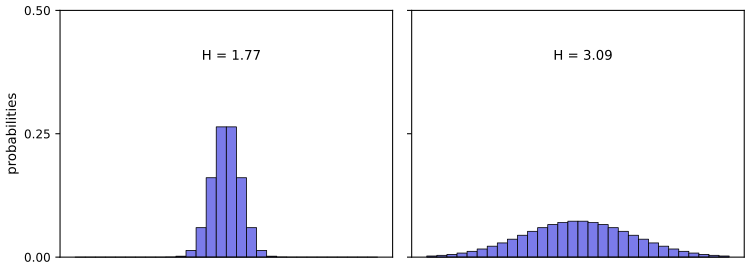
fig_2_14. Download: PDF · SVGResult 2.8 (the uniform distribution has maximum entropy) (2.87), (2.88), Exercises 2.22, 2.23
For a variable with \(M\) states, \(0\le\H[p]\le\ln M\), with \(\H=\ln M\) only for \(p(x_i)=1/M\).
Filling the gap 2.13: the Lagrangian stationary point is the global maximum pp. 48–49
The book maximises \(\widetilde\H=-\sum_ip_i\ln p_i+\lambda(\sum_ip_i-1)\) (2.87) and checks the Hessian \(\partial^2\widetilde\H/\partial p_i\partial p_j=-I_{ij}/p_i\) (2.88). Here is why that settles it, and a second proof by Jensen.
Derivation
Stationary point. \(\partial\widetilde\H/\partial p_i=-\ln p_i-1+\lambda=0\) gives \(p_i=e^{\lambda-1}\), the same for all \(i\); the constraint gives \(p_i=1/M\) and \(\H=\ln M\).
Why it is the maximum. The Hessian \(-\diag(1/p_i)\) is negative definite at every interior point, so \(\widetilde\H\) is strictly concave on the open simplex \(\{p_i>0,\sum p_i=1\}\) (the constraint is linear, so on the simplex \(\widetilde\H=\H\)). A stationary point of a concave function on a convex set is a global maximum there; by continuity of \(\H\) up to the boundary (using \(0\ln0=0\)), boundary points cannot exceed it. A second-derivative test at one point alone would only give a local maximum; it is concavity everywhere that makes it global.
Second proof (Exercise 2.23). \(\ln\) is concave, so by Jensen's inequality (Result 2.10 and gap 2.16) with weights \(p_i\) over the states with \(p_i>0\): \(\H=\sum_ip_i\ln\frac1{p_i}\le\ln\sum_ip_i\frac1{p_i}\le\ln M\). Equality in Jensen for the strictly concave \(\ln\) needs \(1/p_i\) constant, and the last step needs all \(M\) states to be used: \(p_i=1/M\). ∎
2.5.3 Differential entropy
pp. 49–50 Quantise a continuous \(x\) into bins of width \(\Delta\). By the mean value theorem each bin has a point \(x_i\) with \(\int_{i\Delta}^{(i+1)\Delta}p(x)\,\d x=p(x_i)\Delta\) (2.89), and the entropy of the quantised variable is
\[ \H_\Delta=-\sum_ip(x_i)\Delta\ln\big(p(x_i)\Delta\big)=-\sum_ip(x_i)\Delta\ln p(x_i)-\ln\Delta. \tag{2.90} \]Dropping \(-\ln\Delta\) and letting \(\Delta\to0\) defines the differential entropy
\[ \lim_{\Delta\to0}\Big\{-\sum_ip(x_i)\Delta\ln p(x_i)\Big\}=-\int p(x)\ln p(x)\,\d x,\qquad \H[\mathbf{x}]=-\int p(\mathbf{x})\ln p(\mathbf{x})\,\d\mathbf{x}. \tag{2.91, 2.92} \]Filling the gap 2.14: what the limit (2.91) needs, and what differential entropy is not p. 50
Derivation
The limit. The sum in (2.91) is a Riemann sum of \(\psi(x)=-p(x)\ln p(x)\) with tags \(x_i\). If \(p\) is continuous, \(\psi\) is continuous (with \(\psi=0\) where \(p=0\)); on any bounded interval the Riemann sums converge to the integral as \(\Delta\to0\). On the whole line one also needs the tails to be negligible, e.g. \(\int|p\ln p|\,\d x\lt \infty\) together with a monotone tail (true for the Gaussian, the Laplace and most densities used in this book). The code confirms that \(\H_\Delta+\ln\Delta\) converges to (2.99) for a Gaussian as \(\Delta\to0\).
What it is not. \(\H_\Delta\) itself diverges like \(-\ln\Delta\): specifying a real number exactly takes infinitely many bits. The differential entropy is the finite part left over; it can be negative (Result 2.9) and it is not invariant under a change of variables: for \(\mathbf{y}=\mathbf{A}\mathbf{x}\), \(\H[\mathbf{y}]=\H[\mathbf{x}]+\ln|\det\mathbf{A}|\) (Exercise 2.30; this follows from Result 2.7). Differences of differential entropies, such as mutual information and KL divergence, are invariant, because the Jacobian terms cancel. ∎
2.5.4 Maximum entropy
pp. 50–51 Maximise \(-\int p\ln p\) subject to normalisation, mean \(\mu\) and variance \(\sigma^2\) (2.93)–(2.95), using the functional (2.96) with multipliers \(\lambda_1,\lambda_2,\lambda_3\). Setting its functional derivative to zero gives
\[ p(x)=\exp\{-1+\lambda_1+\lambda_2x+\lambda_3(x-\mu)^2\}. \tag{2.97} \]Result 2.9 (the Gaussian maximises differential entropy) (2.98), (2.99), Exercises 2.24, 2.25
Among all densities with mean \(\mu\) and variance \(\sigma^2\), the entropy is largest for \(\N(x\given\mu,\sigma^2)\) (2.98), uniquely, and its value is
\[ \H[x]=\frac12\big\{1+\ln(2\pi\sigma^2)\big\}, \tag{2.99} \]which is negative when \(\sigma^2\lt 1/(2\pi e)\).
Filling the gap 2.15: the multipliers, and a proof that does not need the calculus of variations pp. 50–51
The book says the multipliers "can be found by back-substitution" and that the stationary point is the maximum. Both steps are short; and Gibbs' inequality proves global optimality directly, which the stationarity condition alone does not.
Derivation
The stationary point. For a perturbation \(p\to p+\epsilon\eta\), the first-order change of (2.96) is \(\epsilon\int\eta(x)\{-\ln p(x)-1+\lambda_1+\lambda_2x+\lambda_3(x-\mu)^2\}\d x\) (the derivative of \(p\ln p\) is \(\ln p+1\)). This vanishes for every \(\eta\) only if the brace is zero, which is (2.97).
The multipliers. (2.97) is the exponential of a quadratic, so it is normalisable only if \(\lambda_3\lt 0\); write \(\lambda_3=-1/(2s^2)\). Completing the square shows it is a Gaussian with mean \(\mu+\lambda_2s^2\) and variance \(s^2\). The mean constraint (2.94) forces \(\lambda_2=0\), the variance constraint (2.95) forces \(s^2=\sigma^2\), i.e. \(\lambda_3=-1/(2\sigma^2)\), and normalisation forces \(e^{\lambda_1-1}=(2\pi\sigma^2)^{-1/2}\), i.e. \(\lambda_1=1-\frac12\ln(2\pi\sigma^2)\). (The published solution gives \(\lambda_3=+1/(2\sigma^2)\), which would make (2.97) grow without bound; the code checks both signs.)
Global optimality by Gibbs' inequality. Let \(p\) be any density with mean \(\mu\) and variance \(\sigma^2\) and let \(q=\N(\mu,\sigma^2)\). Using \(\ln q(x)=-\frac12\ln(2\pi\sigma^2)-\frac{(x-\mu)^2}{2\sigma^2}\) and the variance constraint,
\[ 0\le\KL(p\|q)=-\H[p]-\int p\ln q\,\d x=-\H[p]+\tfrac12\ln(2\pi\sigma^2)+\tfrac12=-\H[p]+\H[q]. \]So \(\H[p]\le\H[q]\), with equality only if \(p=q\) (Result 2.10). The same computation with \(p=q\) gives (2.99). Note that non-negativity of \(p\) was never imposed; the solution happens to satisfy it.
Comparison. With variance \(\sigma^2\) the Laplace density has entropy \(1+\ln(2\gamma)\) with \(\gamma=\sigma/\sqrt2\), and the uniform density \(\ln(\sigma\sqrt{12})\); both are below (2.99). For \(\sigma^2=1.3\) the three values are 1.550 (Gaussian), 1.478 (Laplace) and 1.374 (uniform). Full treatment of the same result: companion course, Result 1.21. ∎
2.5.5 Kullback–Leibler divergence
pp. 51–53 If values of \(x\sim p\) are encoded with a code built for \(q\), the average extra information is the relative entropy or KL divergence (Kullback and Leibler, 1951)
\[ \KL(p\|q)=-\int p(x)\ln q(x)\,\d x-\Big(-\int p(x)\ln p(x)\,\d x\Big)=-\int p(x)\ln\Big\{\frac{q(x)}{p(x)}\Big\}\d x , \tag{2.100} \]which is not symmetric. A function is convex if every chord lies on or above it:
\[ f(\lambda a+(1-\lambda)b)\le\lambda f(a)+(1-\lambda)f(b),\qquad 0\le\lambda\le1, \tag{2.101} \]and strictly convex if equality holds only at \(\lambda\in\{0,1\}\) (for \(a\neq b\)).
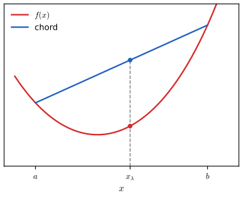
fig_2_15. Download: PDF · SVGBy induction (2.101) gives Jensen's inequality for convex \(f\) and weights \(\lambda_i\ge0\), \(\sum\lambda_i=1\):
\[ f\Big(\sum_{i=1}^{M}\lambda_ix_i\Big)\le\sum_{i=1}^{M}\lambda_if(x_i),\qquad f(\E[x])\le\E[f(x)],\qquad f\Big(\int x\,p(x)\,\d x\Big)\le\int f(x)\,p(x)\,\d x. \tag{2.102–2.104} \]Filling the gap 2.16: convexity and second derivatives, Jensen's inequality and its equality case p. 52, Exercises 2.32, 2.33
The book says convexity "is equivalent to the requirement that the second derivative be everywhere positive" and leaves Jensen to induction. The equivalence needs one correction, and the continuous form (2.104) needs its own argument.
Derivation
Convexity and \(f''\). For twice-differentiable \(f\) on an interval: (i) \(f\) is convex \(\iff f''\ge0\) everywhere; (ii) \(f''>0\) everywhere \(\implies f\) strictly convex; (iii) the converse of (ii) is false: \(f(x)=x^4\) is strictly convex but \(f''(0)=0\). So "positive second derivative" is sufficient for strict convexity, and "non-negative" is equivalent to convexity. Proof of (i), \(\Rightarrow\): convexity makes the slopes of chords increase: for \(a\lt c\lt b\), \(\frac{f(c)-f(a)}{c-a}\le\frac{f(b)-f(c)}{b-c}\) (rearrange (2.101) with \(c=\lambda a+(1-\lambda)b\)); letting \(c\to a\) and \(c\to b\) gives \(f'(a)\le f'(b)\), so \(f'\) is non-decreasing and \(f''\ge0\). \(\Leftarrow\) and (ii): by Taylor's theorem with Lagrange remainder, \(f(x)=f(c)+f'(c)(x-c)+\frac12f''(\xi)(x-c)^2\ge f(c)+f'(c)(x-c)\), strictly if \(f''>0\) and \(x\neq c\). Apply this at \(x=a\) and \(x=b\) with \(c=\lambda a+(1-\lambda)b\), multiply by \(\lambda\) and \(1-\lambda\) and add: the linear terms cancel because \(\lambda(a-c)+(1-\lambda)(b-c)=0\), leaving (2.101), strict when \(f''>0\).
Jensen by induction (Exercise 2.33). \(M=1\) is trivial and \(M=2\) is (2.101). Assume the result for \(M\) points and take \(M+1\) with \(\lambda_{M+1}\lt 1\) (otherwise trivial). Put \(\eta_i=\lambda_i/(1-\lambda_{M+1})\), \(i\le M\), which are non-negative and sum to 1. Then \(\sum_{i\le M+1}\lambda_ix_i=\lambda_{M+1}x_{M+1}+(1-\lambda_{M+1})\sum_{i\le M}\eta_ix_i\); apply (2.101) and then the hypothesis to the inner sum, and multiply back: \(f(\sum\lambda_ix_i)\le\lambda_{M+1}f(x_{M+1})+\sum_{i\le M}\lambda_if(x_i)\).
Continuous form (2.104) via a supporting line. If \(f\) is convex and differentiable, the Taylor argument above gives \(f(x)\ge f(m)+f'(m)(x-m)\) for all \(x\). Take \(m=\E[x]\) and average over \(p\): \(\E[f(x)]\ge f(m)+f'(m)(\E[x]-m)=f(\E[x])\). (Without differentiability a supporting line still exists at every interior point.) If \(f\) is strictly convex the inequality \(f(x)>f(m)+f'(m)(x-m)\) is strict for \(x\neq m\), so equality in Jensen forces \(x=\E[x]\) with probability one. ∎
Result 2.10 (Gibbs' inequality; KL minimisation is maximum likelihood) (2.105), (2.106)
\(\KL(p\|q)\ge0\), with equality if and only if \(p=q\) (almost everywhere). For data \(x_1,\dots,x_N\) drawn from \(p\) and a model \(q(x\given\bm\theta)\),
\[ \KL(p\|q)\simeq\frac1N\sum_{n=1}^{N}\{-\ln q(x_n\given\bm\theta)+\ln p(x_n)\}, \tag{2.106} \]so minimising the KL divergence over \(\bm\theta\) amounts to maximising the log likelihood.
Filling the gap 2.17: the equality case of (2.105), with attention to supports pp. 52–53
Derivation
Let \(S=\{x:p(x)>0\}\). The integral in (2.100) runs over \(S\). Apply Jensen to the strictly convex \(-\ln\) and the random variable \(z=q(x)/p(x)\) with \(x\sim p\):
\[ \KL(p\|q)=\E_p\big[-\ln z\big]\ge-\ln\E_p[z]=-\ln\int_Sq(x)\,\d x\ge-\ln1=0 . \tag{2.105} \]Equality in the first step requires \(z\) to be constant \(p\)-almost surely (strict convexity, gap 2.16), say \(q=cp\) on \(S\); equality in the second requires \(\int_Sq=1\), i.e. \(q\) puts no mass outside \(S\). Together \(c=1\) and \(q=p\) almost everywhere. If \(q=0\) on a set where \(p>0\), \(\KL(p\|q)=+\infty\): the forward KL punishes a model that misses any of the data's support, which is why its minimiser spreads out (the forward versus reverse demo).
KL and maximum likelihood. \(\KL(p\|q_{\bm\theta})=-\E_p[\ln q(x\given\bm\theta)]-\H[p]\); the entropy does not depend on \(\bm\theta\), and the first term is estimated without bias by the sample average (2.106) (gap 2.3), which is \(-\frac1N\) times the log likelihood. Equivalently (Exercise 2.34), the KL divergence from the empirical distribution (2.37) to \(q_{\bm\theta}\) is the negative mean log likelihood plus a constant (an infinite one, formally, since the empirical distribution has no density, which is why one works with the cross-entropy term alone). ∎
2.5.6 Conditional entropy
p. 53 The average additional information needed to specify \(\mathbf{y}\) once \(\mathbf{x}\) is known is the conditional entropy, and the information in the pair splits accordingly:
\[ \H[\mathbf{y}\given\mathbf{x}]=-\iint p(\mathbf{y},\mathbf{x})\ln p(\mathbf{y}\given\mathbf{x})\,\d\mathbf{y}\,\d\mathbf{x},\qquad \H[\mathbf{x},\mathbf{y}]=\H[\mathbf{y}\given\mathbf{x}]+\H[\mathbf{x}]. \tag{2.107, 2.108} \]2.5.7 Mutual information
p. 54 The mutual information is the KL divergence between the joint distribution and the product of the marginals:
\[ \I[\mathbf{x},\mathbf{y}]\equiv\KL\big(p(\mathbf{x},\mathbf{y})\|p(\mathbf{x})p(\mathbf{y})\big)=-\iint p(\mathbf{x},\mathbf{y})\ln\Big(\frac{p(\mathbf{x})p(\mathbf{y})}{p(\mathbf{x},\mathbf{y})}\Big)\d\mathbf{x}\,\d\mathbf{y}. \tag{2.109} \]Result 2.11 (entropy identities) (2.108), (2.110), Exercises 2.29, 2.35, 2.38
\[ \I[\mathbf{x},\mathbf{y}]=\H[\mathbf{x}]-\H[\mathbf{x}\given\mathbf{y}]=\H[\mathbf{y}]-\H[\mathbf{y}\given\mathbf{x}]\ge0, \tag{2.110} \]with \(\I=0\) if and only if \(\mathbf{x}\) and \(\mathbf{y}\) are independent; hence \(\H[\mathbf{x},\mathbf{y}]\le\H[\mathbf{x}]+\H[\mathbf{y}]\) and conditioning never increases entropy on average.
Filling the gap 2.18: proofs of (2.108) and (2.110) pp. 53–54
Derivation
(2.108). Insert \(\ln p(\mathbf{x},\mathbf{y})=\ln p(\mathbf{y}\given\mathbf{x})+\ln p(\mathbf{x})\) into \(\H[\mathbf{x},\mathbf{y}]=-\iint p\ln p\); the second part integrates over \(\mathbf{y}\) by the sum rule to \(-\int p(\mathbf{x})\ln p(\mathbf{x})\,\d\mathbf{x}=\H[\mathbf{x}]\).
(2.110). Write the ratio in (2.109) as \(p(\mathbf{x},\mathbf{y})/(p(\mathbf{x})p(\mathbf{y}))=p(\mathbf{x}\given\mathbf{y})/p(\mathbf{x})\). Then \(\I=\iint p(\mathbf{x},\mathbf{y})\ln p(\mathbf{x}\given\mathbf{y})-\iint p(\mathbf{x},\mathbf{y})\ln p(\mathbf{x})=-\H[\mathbf{x}\given\mathbf{y}]+\H[\mathbf{x}]\), the second integral reducing by the sum rule; symmetrically with \(\mathbf{x}\leftrightarrow\mathbf{y}\). Non-negativity and the equality case are those of the KL divergence (gap 2.17): \(\I=0\iff p(\mathbf{x},\mathbf{y})=p(\mathbf{x})p(\mathbf{y})\). Combining with (2.108), \(\H[\mathbf{x}]+\H[\mathbf{y}]-\H[\mathbf{x},\mathbf{y}]=\I\ge0\) (Exercise 2.29).
Reading. \(\I\) is the reduction in uncertainty about \(\mathbf{x}\) from observing \(\mathbf{y}\); in Bayesian language, the expected information gained about \(\mathbf{x}\) (prior \(p(\mathbf{x})\), posterior \(p(\mathbf{x}\given\mathbf{y})\)) from the observation \(\mathbf{y}\). Unlike the covariance (gap 2.4) it vanishes only under independence. For the companion treatment see Result 1.23 there. ∎
2.6 Bayesian probabilities
See also: Bayesian and Probabilistic Machine Learning, Section 1.2.3 (Bayesian probabilities) and, for the coin with a continuous prior, its Section 2.1.1 (the beta distribution).
pp. 54–55 Probabilities as degrees of belief are not an ad hoc choice: Cox (1946) showed that consistent rules for numerical degrees of belief must be equivalent to the sum and product rules. For the bent coin the unknown is \(Q\) ("the concave side is heads"); Bayes' theorem turns a prior \(p(Q)\) into a posterior given the flips, and the posterior after some flips is the prior for the next ones. A Bayesian treatment also avoids absurd conclusions such as "a coin that showed three heads in three tosses will always land heads", which maximum likelihood draws.
Filling the gap 2.19: updating the bent coin, and why the flips are not independent p. 55, Exercise 2.40
The book says the intuition "is correct, and furthermore, we can quantify this". The quantification has one subtle point, on which the published solution of Exercise 2.40 goes wrong.
Derivation
The coin lands concave side up with probability \(\rho=0.6\). If \(Q=1\), heads means concave up: \(p(H\given Q=1)=\rho\); if \(Q=0\), \(p(H\given Q=0)=1-\rho\). Given \(Q\) the flips are independent, so for a sequence \(\D\) with \(h\) heads and \(t\) tails, \(p(\D\given Q=1)=\rho^h(1-\rho)^t\) and \(p(\D\given Q=0)=(1-\rho)^h\rho^t\). The sum rule then gives
\[ p(\D)=p(\D\given Q=1)\,p(Q=1)+p(\D\given Q=0)\,p(Q=0), \]a mixture, not \(p(H)^h\,p(T)^t\): unconditionally the flips are dependent, because each head is evidence for \(Q=1\) and so raises the probability of the next head. Bayes gives
\[ \frac{p(Q=1\given\D)}{p(Q=0\given\D)}=\Big(\frac{\rho}{1-\rho}\Big)^{h-t}\frac{p(Q=1)}{p(Q=0)}, \]so only \(h-t\) matters, and processing the flips one at a time (each posterior becoming the next prior) gives the same result because the likelihood ratios multiply. The predictive probability of a head is \(p(H\given\D)=\rho\,p(Q=1\given\D)+(1-\rho)\,p(Q=0\given\D)\), by the sum and product rules and the conditional independence of the next flip from \(\D\) given \(Q\). Numbers for Exercise 2.40 are in its solution. ∎
2.6.1 Model parameters
pp. 55–56 Treat the parameters \(\mathbf{w}\) as uncertain, with prior \(p(\mathbf{w})\). The data \(\D\) enter through the likelihood \(p(\D\given\mathbf{w})\), and
\[ p(\mathbf{w}\given\D)=\frac{p(\D\given\mathbf{w})\,p(\mathbf{w})}{p(\D)},\qquad \text{posterior}\propto\text{likelihood}\times\text{prior},\qquad p(\D)=\int p(\D\given\mathbf{w})\,p(\mathbf{w})\,\d\mathbf{w}. \tag{2.111–2.113} \]The likelihood is a function of \(\mathbf{w}\) but not a density over \(\mathbf{w}\): its integral over \(\mathbf{w}\) need not be 1. The negative log likelihood is what the machine learning literature calls an error function. A frequentist treats \(\mathbf{w}\) as fixed and studies an estimator over hypothetical repeated data sets (as in Section 2.3.3); a Bayesian conditions on the one observed data set and expresses uncertainty about \(\mathbf{w}\) by a distribution.
2.6.2 Regularization
See also: Bayesian and Probabilistic Machine Learning, Result 1.10 (MAP estimation is regularised least squares).
pp. 56–57 The maximum a posteriori (MAP) estimate maximises (2.111), i.e. minimises
\[ -\ln p(\mathbf{w}\given\D)=-\ln p(\D\given\mathbf{w})-\ln p(\mathbf{w})+\ln p(\D). \tag{2.114} \]With independent zero-mean Gaussian priors of variance \(s^2\) on the \(M+1\) weights,
\[ p(\mathbf{w}\given s)=\prod_{i=0}^{M}\N(w_i\given0,s^2),\qquad -\ln p(\mathbf{w}\given\D)=-\ln p(\D\given\mathbf{w})+\frac{1}{2s^2}\sum_{i=0}^{M}w_i^2+\const . \tag{2.115, 2.116} \]Result 2.12 (MAP with a Gaussian prior is ridge regression; the Bayesian predictive) (2.117), (2.118), Exercise 2.41
For the regression model (2.66), the MAP weights minimise
\[ E(\mathbf{w})=\frac{1}{2\sigma^2}\sum_{n=1}^{N}\{y(x_n,\mathbf{w})-t_n\}^2+\frac{1}{2s^2}\mathbf{w}^\T\mathbf{w}, \tag{2.117} \]which is the regularised error \(\frac12\sum_n\{y-t_n\}^2+\frac\lambda2\|\mathbf{w}\|^2\) of the book's Section 1.2 times \(1/\sigma^2\), with \(\lambda=\sigma^2/s^2\). The fully Bayesian prediction for a new input averages over the posterior:
\[ p(t\given x,\D)=\int p(t\given x,\mathbf{w})\,p(\mathbf{w}\given\D)\,\d\mathbf{w}. \tag{2.118} \]Filling the gap 2.20: deriving (2.117) and (2.118), and the assumptions behind (2.118) pp. 56–57
Derivation
(2.116) and (2.117). \(-\ln\N(w_i\given0,s^2)=\frac{w_i^2}{2s^2}+\frac12\ln(2\pi s^2)\); summing over \(i\) gives the penalty in (2.116) plus a constant. Substituting \(-\ln p(\D\given\mathbf{w})=\frac{1}{2\sigma^2}\sum_n\{y(x_n,\mathbf{w})-t_n\}^2+\frac N2\ln(2\pi\sigma^2)\) from (2.66) and dropping terms free of \(\mathbf{w}\) (including \(\ln p(\D)\)) gives (2.117). Multiplying by \(\sigma^2>0\) does not move the minimiser, which leaves \(\frac12\sum_n\{y-t_n\}^2+\frac{\sigma^2}{2s^2}\|\mathbf{w}\|^2\): ridge regression with \(\lambda=\sigma^2/s^2\). A tight prior (small \(s^2\)) or noisy data (large \(\sigma^2\)) means strong regularisation. For a polynomial the minimiser is \((\bm\Phi^\T\bm\Phi+\lambda\mathbf{I})^{-1}\bm\Phi^\T\mathsf{t}\); the code checks it against direct minimisation of (2.117).
(2.118). By the sum rule over \(\mathbf{w}\) and the product rule,
\[ p(t\given x,\D)=\int p(t,\mathbf{w}\given x,\D)\,\d\mathbf{w}=\int p(t\given x,\mathbf{w},\D)\,p(\mathbf{w}\given x,\D)\,\d\mathbf{w}. \]Two modelling assumptions reduce this to (2.118): (a) given \(\mathbf{w}\) and \(x\), the new target is independent of the training data, \(p(t\given x,\mathbf{w},\D)=p(t\given x,\mathbf{w})\) (the model (2.64) with i.i.d. noise); (b) the new input alone carries no information about \(\mathbf{w}\), \(p(\mathbf{w}\given x,\D)=p(\mathbf{w}\given\D)\). Plugging in a point estimate replaces the posterior by a delta function at \(\mathbf{w}\ML\) or \(\mathbf{w}_{\rm MAP}\), which ignores the uncertainty in \(\mathbf{w}\) and gives over-confident predictions away from the data. For the linear-Gaussian case the integral is Gaussian and is computed in Result 1.11 of the companion course. ∎
2.6.3 Bayesian machine learning
See also: Bayesian and Probabilistic Machine Learning, Section 1.2.6 (Bayesian curve fitting) and the curve-fitting demo there.
pp. 57–58 MAP is still a single point. The defining feature of a Bayesian method is the integration over parameters in (2.118). It removes over-fitting in principle, and the same averaging over models of different complexity, weighted by their posterior probabilities, prefers models of intermediate complexity (Section 9.6 of the book). The drawback is computational: for networks with millions or billions of parameters the integral is out of reach, and with ample data and a fixed budget it is usually better to train a larger network by regularised maximum likelihood than a smaller one in a Bayesian way. This is the route the rest of the book takes.
Corrections to the book and to the solutions manual
Each item was checked numerically.
| Where | Printed | Correct |
|---|---|---|
| Book, p. 30, after (2.20) | "roughly 96% chance that [they] do not have cancer" | 0.9613 is \(p(T=0)\), the chance of a negative test; \(p(C=0)=0.99\). |
| Book, pp. 44–45, Section 2.4.1 | "around the point \(\mathbf{y}=\mathbf{g}(\mathbf{x})\)"; "The formula (2.77) follows" | With the convention \(\mathbf{x}=\mathbf{g}(\mathbf{y})\) the point is \(\mathbf{y}=\mathbf{g}^{-1}(\mathbf{x})\); the formula is (2.76). |
| Book, p. 52, and Exercise 2.32 | convexity "equivalent to" an everywhere positive second derivative | Convex \(\iff f''\ge0\); \(f''>0\) implies strict convexity but not conversely (\(x^4\)). Gap 2.16. |
| Book, Exercise 2.19 | \(0\le f'(x)\lt \infty\) | \(f'>0\) is needed; otherwise mass piles up into a spike. |
| Book, Exercise 2.30 | \(\H[\mathbf{y}]=\H[\mathbf{x}]+\ln\det\mathbf{A}\) | \(\ln|\det\mathbf{A}|\) (the determinant may be negative). |
| Book, Exercise 2.40 | prior 0.1 that the "convex" side is heads | "concave" was intended (as the manual notes); both readings are solved below. |
| Manual, Solution 2.20 | \(\partial y_i/\partial x_i=1+5\sech^2(x_i)\) | \(1+5\sech^2(5x_i)\) (checked against automatic differentiation). |
| Manual, Solution 2.24 | \(\delta J/\delta p=p(x)+1\); \(\lambda_3=1/(2\sigma^2)\) | \(\ln p(x)+1\); \(\lambda_3=-1/(2\sigma^2)\) (with \(+\) the density is not normalisable). |
| Manual, Solution 2.40 | \(p(\D)=\binom{10}{8}0.42^8\,0.58^2\), posterior 0.825, predictive 0.565 | \(p(\D)\) is a mixture over \(Q\): posterior 0.559, predictive 0.512 (simulation agrees). Exercise 2.40. |
| Manual, Solutions 2.29, 2.30, 2.33 | \(\H=\iint p\ln p\); \(|\mathbf{A}|\) for the determinant; induction base "\(M=1\)" from (2.101) | A minus sign is missing; \(|\det\mathbf{A}|\); (2.101) is the case \(M=2\). |
Exercises
All 41 exercises of Chapter 2 (Bishop and Bishop, 2024, pp. 58–63), restated in my own words, with complete solutions (hidden). Stars give the book's difficulty. Each solution was worked independently and then compared with the official solutions manual; where they disagree, the solution says so, and the numbers are checked in the code.
Exercise 2.1 (★). Redo the screening calculation with prevalence \(p(C=1)=0.001\).
Solution
\(p(T=1)=0.03\times0.999+0.9\times0.001=0.03087\), and \(p(C=1\given T=1)=0.0009/0.03087=90/3087\approx0.029\). In odds: \(30\times\frac1{999}\). A positive result raises the probability thirty-fold but it stays below 3% (gap 2.1).
Exercise 2.2 (★★). Show that for the four Efron dice of Figure 2.16, arranged in a cycle, each die beats the previous one with probability \(2/3\).
Solution
Faces: yellow \(3,3,3,3,3,3\); blue \(4,4,4,4,0,0\); green \(5,5,5,1,1,1\); red \(2,2,2,2,6,6\). No number appears on two dice, so there are no ties, and the rolls are independent. Blue beats yellow when it shows 4: \(4/6=2/3\). Green beats blue when green shows 5 (prob. \(\frac12\), always wins) or shows 1 and blue shows 0 (\(\frac12\cdot\frac13\)): \(\frac23\). Red beats green when red shows 6 (\(\frac13\)) or red shows 2 and green 1 (\(\frac23\cdot\frac12\)): \(\frac23\). Yellow beats red when red shows 2: \(\frac23\). So "beats" is not transitive. (All 36 pairs are enumerated exactly in the code.)
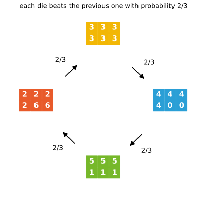
Figure 2.16 (reproduced). The four Efron dice, each shown by its six face values; the arrows point from a die to the one that beats it, labelled with the winning probability computed by enumeration. Reproduces Bishop and Bishop (2024), Figure 2.16. Code: fig_2_16. Download: PDF · SVGExercise 2.3 (★). If \(y=u+v\) with \(u,v\) independent, show that \(p(y)=\int p_u(u)p_v(y-u)\,\d u\) (2.119), the convolution.
Solution
By the sum and product rules, \(p(y)=\int p(y\given u)p_u(u)\,\d u\). Given \(u\), \(y=u+v\) is \(v\) shifted by \(u\); by independence \(v\) still has density \(p_v\), and a shift has Jacobian 1 (Result 2.6), so \(p(y\given u)=p_v(y-u)\). (The manual writes \(p(y\given u,v)=\delta(y-u-v)\) and integrates out \(v\), which is the same.) For two uniforms on \((0,1)\) this gives the triangle \(\min(y,2-y)\) on \((0,2)\), checked by simulation in the code.
Exercise 2.4 (★★). Show that the uniform density (2.33) is normalised and find its mean and variance.
Solution
\(\int_c^d\frac{\d x}{d-c}=1\). \(\E[x]=\frac{d^2-c^2}{2(d-c)}=\frac{c+d}2\); \(\E[x^2]=\frac{d^3-c^3}{3(d-c)}=\frac{c^2+cd+d^2}3\); \(\var[x]=\frac{c^2+cd+d^2}{3}-\frac{(c+d)^2}{4}=\frac{(d-c)^2}{12}\). (The manual switches to \(a,b\) for the end points halfway through.)
Exercise 2.5 (★★). Show that the exponential (2.34) and Laplace (2.35) densities are normalised.
Solution
\(\int_0^\infty\lambda e^{-\lambda x}\d x=[-e^{-\lambda x}]_0^\infty=1\). For the Laplace density substitute \(z=(x-\mu)/\gamma\) (\(\d x=\gamma\,\d z\)): \(\int\frac1{2\gamma}e^{-|x-\mu|/\gamma}\d x=\frac12\int e^{-|z|}\d z=\frac12(1+1)=1\), splitting at \(z=0\).
Exercise 2.6 (★). Show that the empirical density (2.37) is normalised.
Solution
Each \(\delta(x-x_n)\) integrates to 1 (substitute \(y=x-x_n\)), so the average of \(N\) of them integrates to 1. See gap 2.3.
Exercise 2.7 (★). Use (2.37) to justify the approximation (2.40).
Solution
Replacing \(p\) by the empirical distribution of a sample from it, \(\int f(x)\frac1N\sum_n\delta(x-x_n)\d x=\frac1N\sum_nf(x_n)\) by the sifting property. Why the replacement is accurate (unbiasedness, variance \(\var[f]/N\), the law of large numbers) is in gap 2.3.
Exercise 2.8 (★). Show (2.45) from (2.44).
Solution
With \(m=\E[f]\) a constant: \(\E[(f-m)^2]=\E[f^2]-2m\E[f]+m^2=\E[f^2]-m^2\).
Exercise 2.9 (★). Show that independent variables have zero covariance.
Solution
\(\E[xy]=\sum_x\sum_yxy\,p(x)p(y)=\big(\sum_xx\,p(x)\big)\big(\sum_yy\,p(y)\big)=\E[x]\E[y]\), and likewise with integrals; so \(\cov[x,y]=0\). The converse is false (Exercise 2.39).
Exercise 2.10 (★). For independent \(x,z\), show \(\E[x+z]=\E[x]+\E[z]\) (2.120) and \(\var[x+z]=\var[x]+\var[z]\) (2.121).
Solution
The first is linearity of the integral (independence is not needed). For the second, \((x+z-\E[x+z])^2=(x-\E x)^2+(z-\E z)^2+2(x-\E x)(z-\E z)\); the expectation of the last term is \(2\cov[x,z]=0\) by Exercise 2.9.
Exercise 2.11 (★). Prove \(\E[x]=\E_y[\E_x[x\given y]]\) (2.122) and \(\var[x]=\E_y[\var_x[x\given y]]+\var_y[\E_x[x\given y]]\) (2.123).
Solution
\(\E_y[\E_x[x\given y]]=\int p(y)\int x\,p(x\given y)\,\d x\,\d y=\iint x\,p(x,y)\,\d x\,\d y=\E[x]\), by the product and sum rules; the same holds with \(x^2\). Write \(m(y)=\E[x\given y]\). Then \(\E_y[\var[x\given y]]=\E_y[\E[x^2\given y]]-\E_y[m^2]=\E[x^2]-\E_y[m^2]\) and \(\var_y[m]=\E_y[m^2]-(\E_y[m])^2=\E_y[m^2]-\E[x]^2\). Adding, the \(\E_y[m^2]\) terms cancel and the sum is \(\E[x^2]-\E[x]^2=\var[x]\). (The total variance splits into the average spread within groups and the spread of the group means.)
Exercise 2.12 (★★★). Evaluate \(I=\int e^{-x^2/2\sigma^2}\d x\) (2.124) by squaring it (2.125) and changing to polar coordinates, and deduce that the Gaussian is normalised.
Solution
With \(x=r\cos\theta\), \(y=r\sin\theta\), the Jacobian determinant is \(\det\begin{pmatrix}\cos\theta&-r\sin\theta\\ \sin\theta&r\cos\theta\end{pmatrix}=r\), and the plane is covered once by \(r\ge0\), \(\theta\in[0,2\pi)\). So \(I^2=\int_0^{2\pi}\int_0^\infty e^{-r^2/2\sigma^2}r\,\d r\,\d\theta=2\pi\int_0^\infty e^{-u/2\sigma^2}\frac{\d u}2=2\pi\sigma^2\) with \(u=r^2\), hence \(I=(2\pi\sigma^2)^{1/2}\) (2.126) (\(I>0\)). Substituting \(y=x-\mu\), \(\int\N(x\given\mu,\sigma^2)\d x=I/(2\pi\sigma^2)^{1/2}=1\). (Squaring is legitimate because the integrand is positive and integrable, so Fubini applies.)
Exercise 2.13 (★★). Verify (2.52) by a change of variables and (2.53) by differentiating the normalisation condition (2.127) with respect to \(\sigma^2\); deduce (2.54).
Solution
See the proof under Result 2.2: with \(z=x-\mu\), the odd part integrates to zero and \(\E[x]=\mu\). Differentiating \(\int e^{-(x-\mu)^2/2\sigma^2}\d x=(2\pi\sigma^2)^{1/2}\) under the integral sign (justified by dominated convergence) gives \(\E[(x-\mu)^2]=\sigma^2\), so \(\E[x^2]=\sigma^2+2\mu\E[x]-\mu^2=\mu^2+\sigma^2\) and \(\var[x]=\sigma^2\). The code checks the derivative identity by finite differences.
Exercise 2.14 (★). Show that the Gaussian's mode is \(\mu\).
Solution
\(\frac{\d}{\d x}\N(x\given\mu,\sigma^2)=-\frac{x-\mu}{\sigma^2}\N(x\given\mu,\sigma^2)\) is positive for \(x\lt \mu\), zero at \(\mu\) and negative for \(x>\mu\), so \(\mu\) is the unique global maximum.
Exercise 2.15 (★). Derive (2.57) and (2.58) by setting the derivatives of (2.56) to zero.
Solution
\(\partial\ell/\partial\mu=\frac1{\sigma^2}\sum_n(x_n-\mu)=0\) gives \(\mu\ML=\bar x\); \(\partial\ell/\partial\sigma^2=\frac{1}{2\sigma^4}\sum_n(x_n-\mu)^2-\frac{N}{2\sigma^2}=0\) gives \(\sigma^2=\frac1N\sum_n(x_n-\mu)^2\), evaluated at \(\mu=\mu\ML\). That this stationary point is the global maximum is gap 2.5.
Exercise 2.16 (★★). Show \(\E[x_nx_m]=\mu^2+I_{nm}\sigma^2\) (2.128) and hence (2.59), (2.60).
Solution
For \(n=m\), \(\E[x_n^2]=\mu^2+\sigma^2\) by (2.53); for \(n\neq m\) independence gives \(\E[x_n]\E[x_m]=\mu^2\). Then \(\E[\mu\ML]=\frac1N\sum\E[x_n]=\mu\), and expanding \(\sigma^2\ML=\frac1N\sum_nx_n^2-\mu\ML^2\):
\[ \E[\sigma^2\ML]=(\mu^2+\sigma^2)-\frac{1}{N^2}\sum_{n,m}\E[x_nx_m]=(\mu^2+\sigma^2)-\Big(\mu^2+\frac{\sigma^2}{N}\Big)=\frac{N-1}{N}\sigma^2 . \]A shorter route is in gap 2.6.
Exercise 2.17 (★★). Prove (2.62): the estimator (2.61) that uses the true mean is unbiased.
Solution
\(\E[(x_n-\mu)^2]=\var[x_n]=\sigma^2\) for each \(n\), so \(\E[\hat\sigma^2]=\frac1N\cdot N\sigma^2=\sigma^2\). (No Gaussian assumption is needed, only a finite variance.)
Exercise 2.18 (★). Maximise (2.66) over \(\sigma^2\) to obtain (2.68).
Solution
\(\frac{\partial}{\partial\sigma^2}\ln p=\frac{1}{2\sigma^4}\sum_n\{y(x_n,\mathbf{w})-t_n\}^2-\frac{N}{2\sigma^2}=0\) gives \(\sigma^2=\frac1N\sum_n\{y(x_n,\mathbf{w})-t_n\}^2\), evaluated at \(\mathbf{w}\ML\) (which does not depend on \(\sigma^2\), Result 2.5). The profile argument of gap 2.5 shows it is the maximum.
Exercise 2.19 (★★). Show that any density \(p(y)\) can be obtained from a fixed positive density \(q(x)\) by a monotonic change of variable \(y=f(x)\); write the differential equation for \(f\) and sketch the transformation.
Solution
Take \(f=P^{-1}\circ Q\) (CDFs \(P\), \(Q\)); then \(P(f(x))=Q(x)\) and \(p(f(x))\,f'(x)=q(x)\) is the differential equation, with \(f'>0\) required. Full argument in gap 2.7. For the sketch: plot \(q\) on the \(x\) axis, the increasing curve \(y=f(x)\), and \(p\) on the \(y\) axis; \(f\) is steep where \(q\) is large relative to \(p\) (mass is spread out) and flat where \(p\) is large (mass is concentrated), exactly the layout of Figure 2.12; the change-of-variables demo draws it interactively. The code checks the construction by turning Gaussian samples into exponential ones.
Exercise 2.20 (★). Find the Jacobian of (2.78)–(2.79).
Solution
\(\partial y_1/\partial x_1=1+5\sech^2(5x_1)\), \(\partial y_1/\partial x_2=0\), \(\partial y_2/\partial x_1=x_1^2\), \(\partial y_2/\partial x_2=1+5\sech^2(5x_2)\); the determinant is the product of the diagonal entries. The solutions manual writes \(\sech^2(x_i)\), dropping the factor 5 inside the argument (the chain rule gives \(\frac{\d}{\d u}\tanh(5u)=5\sech^2(5u)\)); automatic differentiation confirms the version here. Invertibility and the transformed density: gap 2.9.
Exercise 2.21 (★). From \(h(p^2)=2h(p)\) and additivity, show \(h(p^n)=nh(p)\), \(h(p^{n/m})=\frac nmh(p)\), extend to real exponents by continuity, and conclude \(h(p)\propto\ln p\).
Solution
Additivity for independent events with probabilities \(p\) and \(q\) is \(h(pq)=h(p)+h(q)\); induction gives \(h(p^n)=nh(p)\); applying it to \(p^{1/m}\) gives \(h(p)=mh(p^{1/m})\), so \(h(p^{n/m})=\frac nmh(p)\). Continuity (or monotonicity) extends this to \(h(p^x)=xh(p)\) for real \(x>0\). For any \(p\in(0,1)\) write \(p=e^{-u}\), \(u=-\ln p\): \(h(p)=h((e^{-1})^u)=u\,h(e^{-1})=-h(e^{-1})\ln p\). A fully rigorous version is gap 2.10.
Exercise 2.22 (★). Use a Lagrange multiplier to show that the entropy (2.86) is maximised by the uniform distribution, with value \(\ln M\).
Solution
Stationarity of (2.87) gives \(\ln p_i=\lambda-1\) for all \(i\), so \(p_i=1/M\) and \(\H=\ln M\). Why this stationary point is the global maximum: gap 2.13.
Exercise 2.23 (★). Use Jensen's inequality (2.102) to show \(\H[x]\le\ln M\).
Solution
\(\ln\) is concave, so Jensen applies with the inequality reversed: \(\H=\sum_ip_i\ln\frac1{p_i}\le\ln\sum_{i:p_i>0}p_i\frac1{p_i}\le\ln M\). Equality case: gap 2.13.
Exercise 2.24 (★★). Show that the stationary point of (2.96) is (2.97), then use the constraints to obtain the Gaussian (2.98).
Solution
See gap 2.15: the first variation gives (2.97); normalisability forces \(\lambda_3\lt 0\), and the constraints give \(\lambda_1=1-\frac12\ln(2\pi\sigma^2)\), \(\lambda_2=0\), \(\lambda_3=-\frac{1}{2\sigma^2}\). The manual's functional derivative of \(\int p\ln p\) should read \(\ln p(x)+1\), its \(\lambda_3\) has the wrong sign, and its remark about "(1.108)" refers to equation numbers of a different book; the exercise as printed here is correct.
Exercise 2.25 (★). Show that the entropy of the Gaussian is (2.99).
Solution
\(-\ln\N(x\given\mu,\sigma^2)=\frac12\ln(2\pi\sigma^2)+\frac{(x-\mu)^2}{2\sigma^2}\); averaging and using (2.95), \(\H=\frac12\ln(2\pi\sigma^2)+\frac12\).
Exercise 2.26 (★★). For fixed \(p(\mathbf{x})\), minimise \(\KL(p\|q)\) over Gaussians \(q=\N(\mathbf{x}\given\bm\mu,\bm\Sigma)\): show \(\bm\mu=\E_p[\mathbf{x}]\) and \(\bm\Sigma=\cov_p[\mathbf{x}]\).
Solution
Up to terms free of \(q\), \(\KL(p\|q)=-\E_p[\ln q]=\frac12\ln|\bm\Sigma|+\frac12\E_p[(\mathbf{x}-\bm\mu)^\T\bm\Sigma^{-1}(\mathbf{x}-\bm\mu)]+\const\). With \(\mathbf{m}=\E_p[\mathbf{x}]\) and \(\mathbf{S}=\cov_p[\mathbf{x}]\), the expectation equals \(\Tr(\bm\Sigma^{-1}\mathbf{S})+(\mathbf{m}-\bm\mu)^\T\bm\Sigma^{-1}(\mathbf{m}-\bm\mu)\). The second term is minimised (to 0) by \(\bm\mu=\mathbf{m}\) for any \(\bm\Sigma\). Then, with \(\bm\Lambda=\bm\Sigma^{-1}\), minimise \(-\frac12\ln|\bm\Lambda|+\frac12\Tr(\bm\Lambda\mathbf{S})\): its gradient \(-\frac12\bm\Lambda^{-1}+\frac12\mathbf{S}\) vanishes at \(\bm\Sigma=\mathbf{S}\), and the function is convex in \(\bm\Lambda\) (\(-\ln|\cdot|\) is convex on positive definite matrices), so this is the minimum (assuming \(\mathbf{S}\) is positive definite). Forward KL fitting is moment matching; the code confirms it numerically for a bimodal \(p\), and the demo compares it with the reverse direction.
Exercise 2.27 (★★). Compute \(\KL(p\|q)\) for \(p=\N(\mu,\sigma^2)\), \(q=\N(m,s^2)\).
Solution
\(-\E_p[\ln q]=\frac12\ln(2\pi s^2)+\frac{\sigma^2+(\mu-m)^2}{2s^2}\) (using \(\E_p[(x-m)^2]=\sigma^2+(\mu-m)^2\)), and \(\E_p[\ln p]=-\H[p]=-\frac12(1+\ln2\pi\sigma^2)\). Adding,
\[ \KL(p\|q)=\frac12\Big\{\ln\frac{s^2}{\sigma^2}+\frac{\sigma^2+(\mu-m)^2}{s^2}-1\Big\}, \]zero only when \(\mu=m\), \(\sigma^2=s^2\) (since \(t-1-\ln t\ge0\) with equality only at \(t=1\)). E.g. \(\KL(\N(0,1)\|\N(1,4))=0.443\) but \(\KL(\N(1,4)\|\N(0,1))=1.307\).
Exercise 2.28 (★★). For the alpha family \(D_\alpha(p\|q)=\frac{4}{1-\alpha^2}\big(1-\int p^{(1+\alpha)/2}q^{(1-\alpha)/2}\d x\big)\) (2.129), show that \(\alpha\to1\) gives \(\KL(p\|q)\) and \(\alpha\to-1\) gives \(\KL(q\|p)\).
Solution
Let \(\alpha=1-\epsilon\). Then \(p^{(1+\alpha)/2}q^{(1-\alpha)/2}=p\,(q/p)^{\epsilon/2}=p\{1+\frac\epsilon2\ln\frac qp+O(\epsilon^2)\}\), so the integral is \(1+\frac\epsilon2\int p\ln\frac qp+O(\epsilon^2)\) (using \(\int p=1\)), and \(1-\alpha^2=2\epsilon-\epsilon^2\). Hence \(D_\alpha=\frac{4}{2\epsilon+O(\epsilon^2)}\big(-\frac\epsilon2\int p\ln\frac qp+O(\epsilon^2)\big)\to-\int p\ln\frac qp=\KL(p\|q)\). The case \(\alpha=-1+\epsilon\) is the same with \(p\) and \(q\) exchanged. (The expansion under the integral needs, e.g., \(\int p|\ln(q/p)|^2\lt \infty\).) Checked numerically in the code.
Exercise 2.29 (★★). Show \(\H[x,y]\le\H[x]+\H[y]\) (2.130), with equality if and only if \(x\) and \(y\) are independent.
Solution
By (2.108) and (2.110), \(\H[x]+\H[y]-\H[x,y]=\H[y]-\H[y\given x]=\I[x,y]\ge0\), and \(\I=0\) exactly under independence (gap 2.18).
Exercise 2.30 (★). For a non-singular linear map \(\mathbf{y}=\mathbf{A}\mathbf{x}\), show \(\H[\mathbf{y}]=\H[\mathbf{x}]+\ln|\det\mathbf{A}|\).
Solution
By Result 2.7, \(p_{\mathbf{y}}(\mathbf{y})=p_{\mathbf{x}}(\mathbf{A}^{-1}\mathbf{y})/|\det\mathbf{A}|\). Then \(\H[\mathbf{y}]=-\E[\ln p_{\mathbf{y}}(\mathbf{y})]=-\E[\ln p_{\mathbf{x}}(\mathbf{x})]+\ln|\det\mathbf{A}|\). The book prints \(\ln\det\mathbf{A}\), which is undefined when \(\det\mathbf{A}\lt 0\); the code checks the formula for Gaussians with a negative determinant.
Exercise 2.31 (★★). If \(\H[y\given x]=0\) for discrete \(x,y\), show that \(y\) is a function of \(x\) wherever \(p(x)>0\).
Solution
\(\H[y\given x]=\sum_xp(x)\sum_y\{-p(y\given x)\ln p(y\given x)\}\) is a sum of non-negative terms, so every term with \(p(x)>0\) vanishes. \(-t\ln t=0\) on \([0,1]\) only at \(t\in\{0,1\}\), and the \(p(y\given x)\) sum to 1, so exactly one \(y\) has \(p(y\given x)=1\).
Exercise 2.32 (★). Show that "every chord lies above the function" (strict convexity) is equivalent to a positive second derivative.
Solution
As stated, the equivalence is false: \(f''>0\) implies strict convexity, and strict convexity implies \(f''\ge0\), but \(x^4\) is strictly convex with \(f''(0)=0\). Proofs of both true directions: gap 2.16. (The manual's proof correctly arrives at \(f''\ge0\) in one direction and assumes \(f''>0\) in the other, so it proves the corrected statement.)
Exercise 2.33 (★★). Prove Jensen's inequality (2.102) from (2.101) by induction.
Solution
See gap 2.16: renormalise the first \(M\) weights by \(1-\lambda_{M+1}\), apply (2.101) and then the induction hypothesis. The base case is \(M=2\), which is (2.101) itself (the manual calls it \(M=1\)).
Exercise 2.34 (★). Show that, up to a constant, the KL divergence from the empirical distribution (2.37) to \(q(x\given\bm\theta)\) is the negative log likelihood.
Solution
\(\KL(p\|q)=-\int p\ln q+\int p\ln p\); the second term does not depend on \(\bm\theta\), and with \(p\) the empirical distribution the first is \(-\frac1N\sum_n\ln q(x_n\given\bm\theta)\) by the sifting property. (Strictly, \(\int p\ln p\) is not finite for a sum of deltas; the statement is about the \(\bm\theta\)-dependent part, see gap 2.17.)
Exercise 2.35 (★). Prove (2.108) from (2.107) and the product rule.
Solution
\(-\iint p(x,y)\ln p(x,y)=-\iint p(x,y)\ln p(y\given x)-\iint p(x,y)\ln p(x)=\H[y\given x]+\H[x]\), integrating \(y\) out of the last term.
Exercise 2.36 (★★★). For binary \(x,y\) with \(p(0,0)=p(0,1)=p(1,1)=\frac13\), \(p(1,0)=0\), compute \(\H[x]\), \(\H[y]\), \(\H[y\given x]\), \(\H[x\given y]\), \(\H[x,y]\), \(\I[x,y]\), and draw the relationships as a diagram.
Solution
Marginals: \(p(x=0)=\frac23\), \(p(x=1)=\frac13\); \(p(y=0)=\frac13\), \(p(y=1)=\frac23\). Conditionals: given \(x=0\), \(y\) is uniform; given \(x=1\), \(y=1\); given \(y=0\), \(x=0\); given \(y=1\), \(x\) is uniform. Hence
(a), (b) \(\H[x]=\H[y]=-\frac23\ln\frac23-\frac13\ln\frac13=\ln3-\frac23\ln2\approx0.6365\); (c), (d) \(\H[y\given x]=\H[x\given y]=\frac23\ln2\approx0.4621\); (e) \(\H[x,y]=\ln3\approx1.0986\); (f) \(\I[x,y]=\H[x]-\H[x\given y]=\ln3-\frac43\ln2\approx0.1744\) nats.
Diagram: two overlapping discs of "sizes" \(\H[x]\) and \(\H[y]\); the overlap is \(\I[x,y]\), the two crescents are \(\H[x\given y]\) and \(\H[y\given x]\), and the union is \(\H[x,y]=\H[x\given y]+\I+\H[y\given x]\). The demo draws it as overlapping bars. Agrees with the manual.
Exercise 2.37 (★). Use Jensen with \(f=\ln\) to show that the arithmetic mean of positive numbers is at least their geometric mean.
Solution
\(\ln\) is concave, so \(\ln\big(\frac1K\sum_kx_k\big)\ge\frac1K\sum_k\ln x_k=\ln\big(\prod_kx_k\big)^{1/K}\); exponentiate (\(\exp\) is increasing). Equality iff all \(x_k\) are equal (strict concavity).
Exercise 2.38 (★). Prove (2.110) from the sum and product rules.
Solution
See gap 2.18: write \(p(x,y)/(p(x)p(y))=p(y\given x)/p(y)\) and integrate.
Exercise 2.39 (★★). Show that independent \(z_1,z_2\) have a diagonal covariance matrix, and that \(y_1\) symmetric about 0 and \(y_2=y_1^2\) are dependent but also uncorrelated.
Solution
The off-diagonal entry is \(\cov[z_1,z_2]=0\) by Exercise 2.9. For the counterexample: \(p(y_2\given y_1)=\delta(y_2-y_1^2)\) depends on \(y_1\), yet \(\cov[y_1,y_2]=\int p(y_1)\,y_1(y_1^2-\E[y_2])\,\d y_1=\E[y_1^3]-\E[y_1]\E[y_1^2]=0\) by symmetry (assuming \(\E|y_1|^3\lt \infty\)). Zero correlation does not imply independence (gap 2.4; simulated in the code).
Exercise 2.40 (★). The bent coin lands concave side up with probability 0.6. With a prior of 0.1 that the concave side is heads (the printed "convex" is a slip), and data of 8 heads and 2 tails in 10 flips, find the posterior probability that the concave side is heads and the probability that the next flip is heads.
Solution
Using gap 2.19 with \(\rho=0.6\), \(h-t=6\): posterior odds \(=1.5^6\times\frac{0.1}{0.9}=11.39\times0.111=1.266\), so
\[ p(Q=1\given\D)=\frac{0.1\times0.6^8\,0.4^2}{0.1\times0.6^8\,0.4^2+0.9\times0.4^8\,0.6^2}=0.5586,\qquad p(H\given\D)=0.6\times0.5586+0.4\times0.4414=0.5117. \]The prior predictive was \(0.6\times0.1+0.4\times0.9=0.42\); the heads in the data raise it to 0.51. The published solution is wrong here. It computes the evidence as \(p(\D)=\binom{10}{8}0.42^8\,0.58^2\), which treats the flips as independent with \(p(H)=0.42\); but they are independent only given \(Q\), and the correct evidence is the mixture over \(Q\). Its posterior 0.825 is not a probability consistent with the model (the posteriors for \(Q=1\) and \(Q=0\) computed that way do not add to 1: \(0.825+0.9\times0.4^8\,0.6^2/(0.42^8\,0.58^2)=0.825+0.652\)). A simulation of two million coins confirms 0.559: among coins showing 8 heads in 10 flips, 55.9% have \(Q=1\). With the exercise read literally (prior 0.1 that the convex side is heads, i.e. 0.9 that the concave side is), the same method gives \(p(Q=1\given\D)=0.9903\) and \(p(H\given\D)=0.5981\).
Exercise 2.41 (★). Derive (2.117) by substituting (2.115) into (2.114) and using (2.66).
Solution
See gap 2.20: the prior contributes \(\frac{1}{2s^2}\mathbf{w}^\T\mathbf{w}\) plus a constant, the likelihood \(\frac1{2\sigma^2}\sum_n\{y(x_n,\mathbf{w})-t_n\}^2\) plus a constant, and \(\ln p(\D)\) is constant in \(\mathbf{w}\).
Demonstrations for this chapter
Each demonstration runs in the browser, with seeded random numbers so that a class sees the same pictures, and links back to these notes. The ▶ Demo boxes above open them already set to the case under discussion. Every number they display was compared with the Python code (the largest discrepancy is \(2\times10^{-8}\), in the iterative reverse-KL fit; all others agree to machine precision).
| Demonstration | What you can see | Sections and results |
|---|---|---|
| Bayes' theorem: medical screening and the bent coin | 10,000 screened people split by disease and test result, the posterior against prevalence after one to three positive tests, and Bayesian updating for the bent coin. Presets: 1 the book's example; 2 prevalence 0.1%; 3 two positive tests; 4 a useless test; 5 the bent coin of Exercise 2.40. | 2.1, 2.6; Result 2.1, gap 2.1, gap 2.19 |
| Gaussian maximum likelihood and the bias of the variance | The likelihood as a product of heights, the log-likelihood surface over \((\mu,\sigma)\), and thousands of simulated data sets showing the \((N-1)/N\) bias and the \(\chi^2_{N-1}\) law. Presets: 1 a poor guess; 2 the maximum (Fig. 2.9); 3 three data sets of two points (Fig. 2.10); 4 2,000 data sets, \(N=2\); 5 \(N=10\). | 2.3.2, 2.3.3; Results 2.3, 2.4 |
| Change of variables: the Jacobian and the moving mode | A Gaussian pushed through a sigmoid or a linear map with transformed histograms, the density with and without the Jacobian factor and the mode equation; in two dimensions the map (2.78)–(2.79) on a grid, samples and the density, with a probe square whose image area matches \(\det\mathbf{J}\). Presets: 1 Fig. 2.12; 2 linear map; 3 steep sigmoid; 4 Fig. 2.13; 5 pure shear. | 2.4, 2.4.1; Results 2.6, 2.7, gap 2.8 |
| Entropy, KL divergence and mutual information | Entropy of narrow and broad distributions against \(\ln M\), the two KL divergences between Gaussians and their integrands, forward and reverse KL fits to a bimodal density, and the information quantities of a 2×2 table. Presets: 1 \(\H=1.77\); 2 \(\H=3.09\) (Fig. 2.14); 3 KL asymmetry; 4 forward versus reverse KL; 5 Exercise 2.36. | 2.5; Results 2.8, 2.10, 2.11 |
The Python code that produces every figure of this page is code/ch02_probabilities.py (see the code index).
References
- Bishop, C. M. and Bishop, H. (2024). Deep Learning: Foundations and Concepts. Springer, Cham. Chapter 2, pp. 23–63. doi:10.1007/978-3-031-45468-4. Book website: www.bishopbook.com.
- Bishop, C. M. (2006). Pattern Recognition and Machine Learning. Springer, New York.
- Cover, T. M. and Thomas, J. A. (1991). Elements of Information Theory. Wiley, New York.
- Cox, R. T. (1946). Probability, frequency and reasonable expectation. American Journal of Physics, 14(1), 1–13.
- Feller, W. (1966). An Introduction to Probability Theory and its Applications, Volume 2. Wiley, New York.
- Kullback, S. and Leibler, R. A. (1951). On information and sufficiency. Annals of Mathematical Statistics, 22(1), 79–86.
- MacKay, D. J. C. (2003). Information Theory, Inference and Learning Algorithms. Cambridge University Press.
- McMillan, B. (1956). Two inequalities implied by unique decipherability. IRE Transactions on Information Theory, 2(4), 115–116.
- Shannon, C. E. (1948). A mathematical theory of communication. Bell System Technical Journal, 27(3), 379–423 and 27(4), 623–656.
The numerical statements in the text (screening posteriors, the Efron dice, the mode of the transformed density, Jacobians against automatic differentiation, entropies, KL divergences, the bent-coin posterior and its simulation) come from short Python computations written for these notes.