Chapter 2. Statistical Modeling
Chapter 1 started from a known model and computed probabilities of data. This chapter goes the other way: from data to a model and its parameters. It fits count distributions and checks the fit (rootograms, chi-square statistics, QQ plots), estimates parameters by maximum likelihood (Poisson, binomial, multinomial, Hardy-Weinberg, Markov chains), tests structured hypotheses by simulation and permutation (nucleotide bias, Chargaff's rule), and then treats the unknown proportion as a random quantity with a Beta prior. It ends with two genomic case studies: motif counts along the E. coli genome and Markov-chain scores that tell CpG islands from the rest of human chromosome 8. The notes follow Holmes and Huber (2019), Chapter 2, and fill in every derivation the book states without proof.
Ch. 1 Discrete data Ch. 2 Statistical modeling Ch. 3 Data visualization Ch. 4 Mixture models Ch. 5 Clustering Ch. 6 Testing Ch. 7 Multivariate analysis Ch. 8 Count data and GLMs Ch. 9 Heterogeneous data Ch. 10 Networks and trees Ch. 11 Image data Ch. 12 Supervised learning Ch. 13 Experimental design
How to read these notes
They follow the book. Sections carry the book's numbers (2.3, 2.9.5, ...), displayed equations that appear in the book carry its numbers, e.g. (2.4), and figures carry the book's figure numbers, so the notes can be read next to the book. Equations without a number are steps that the book skips.
Filling the gaps. The book is applied and often states a result ("the sample mean maximizes the likelihood", "the posterior is also a Beta", "the statistic has a chi-square distribution with 30 degrees of freedom") with a simulation as its only support. Each such place has an orange Filling the gap box with a complete derivation: assumptions, every step, and a numerical confirmation from the course code. Derivations start hidden; open one with its bar or with the button below.
Figures and demonstrations. Every figure computed from data or by simulation is reproduced by ch02_statistical_modeling.R. The ▶ Demo boxes open an interactive demonstration already set to the case being discussed.
Main reference
S. Holmes and W. Huber, Modern Statistics for Modern Biology, Cambridge University Press (2019), Chapter 2, "Statistical Modeling". Section, equation, figure, question and exercise numbers below refer to this book. Further references are listed at the end.
The explanations, derivations and code are my own; the book's results, data sets and figures are cited by their numbers.
The chapter at a glance
- 2.2–2.4 Probability goes from a model to data, statistics from data to a model. For the epitope counts a rootogram suggests a Poisson model, whose maximum-likelihood estimate is the sample mean (Result 2.1); for binomial data it is the observed proportion (Result 2.2). The curvature of the log-likelihood is the Fisher information, which gives standard errors and confidence intervals.
- 2.5–2.6 The multinomial MLE is the vector of observed frequencies (Result 2.3). Pearson's statistic is asymptotically chi-square with \(K-1\) degrees of freedom (Result 2.4), and one degree is lost for every estimated parameter, which corrects the book's 30 to 27 for the ten genes (Filling the gap 2.8).
- 2.7–2.8 A permutation test confirms Chargaff's rule (its exact p-value is \(1/6561\)), a two-way table tests independence, the Hardy-Weinberg MLE is gene counting, a sequence logo displays a product of multinomials, and a Markov chain's transition matrix is estimated row by row.
- 2.9 With a \(\BetaD(\alpha,\beta)\) prior and \(y\) successes in \(n\) trials, the posterior is \(\BetaD(\alpha+y,\beta+n-y)\); its mean shrinks the observed proportion towards the prior mean, data can be added sequentially, and the marginal law of \(Y\) is beta-binomial.
- 2.10 Motif counts in windows look Poisson and the gaps between motifs look exponential; a log-likelihood-ratio score between two Markov chains separates CpG islands from the rest of the genome.
Notation. Data \(x_1,\dots,x_n\); a parametric family \(f(x\given\theta)\); the likelihood \(L(\theta)=\prod_i f(x_i\given\theta)\) and log-likelihood \(\ell(\theta)=\log L(\theta)\); estimates carry hats. \(\Pois(\lambda)\), \(\Bin(n,p)\), \(\Mult(n,\bm p)\) and \(\BetaD(\alpha,\beta)\) are the Poisson, binomial, multinomial and Beta laws; \(\chi^2_\nu\) is the chi-square law with \(\nu\) degrees of freedom; \(\log\) is the natural logarithm unless a base is written.
Prerequisites. Chapter 1 of the course (the Poisson, binomial and multinomial distributions, simulation, the epitope example), basic calculus and the central limit theorem.
2.2 The difference between statistical and probabilistic models
Section 2.2 In Chapter 1 the model was fully specified: false positives in the epitope assay occurred independently with a known rate, so the number of positives per position was \(\Pois(0.5)\), and the probability of seeing a maximum of 7 or more among 100 positions could be deduced (about \(10^{-4}\)). That is a probabilistic computation: model and parameters known, data random. In a statistical problem the direction is reversed. The data are observed, and the family of distributions, its parameters, or both, have to be inferred from them. The book's Figure 2.1 (a schematic, not reproduced) shows the deductive direction; the figure in its margin shows the inductive one, from data \(X\) up to an estimate \(\widehat\theta\).
Definition 2.1 (statistical model, estimator) Sections 2.2–2.3
A parametric statistical model is a family \(\{f(\cdot\given\theta):\theta\in\Theta\}\) of probability distributions for the data, indexed by a parameter \(\theta\) in a set \(\Theta\subseteq\R^d\) of small dimension \(d\). The data \(x=(x_1,\dots,x_n)\) are regarded as one realisation from \(f(\cdot\given\theta_0)\) for some unknown \(\theta_0\). An estimator is any function \(\widehat\theta=\widehat\theta(x)\) of the data with values in \(\Theta\); because the data are random, so is \(\widehat\theta\), and its distribution (its sampling distribution) describes how far it can be from \(\theta_0\).
Two separate decisions are involved: the choice of the family (Poisson, binomial, normal, ...), checked by goodness of fit, and the choice of \(\theta\) within the family, done by estimation. The rest of the chapter does both, in that order for the epitope data.
2.3 A simple example of statistical modeling
Start with the data
Section 2.3 The epitope data e100 of Chapter 1 are the numbers of positive calls at 100 positions of a protein, summed over 50 patients: 58 positions with 0 positives, 34 with 1, 7 with 2 and one position with 7. The book first removes the extreme value, giving e99, to choose a family without being misled by one point, and then returns to all 100 values for estimation.
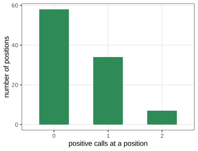
fig_2_2. Reproduces Holmes and Huber (2019), Figure 2.2. PDF · SVGGoodness of fit: visual evaluation
A bar chart alone does not say which distribution fits. A rootogram compares the observed frequencies \(O_k\) of each value \(k\) with the frequencies \(E_k\) expected under a fitted model, on the square-root scale. In the hanging version a bar of height \(\sqrt{O_k}\) hangs from the point \(\sqrt{E_k}\), so the bottom of the bar sits at \(\sqrt{E_k}-\sqrt{O_k}\): when the model is right every bar ends near the horizontal axis.
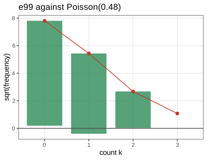
e99 against the Poisson distribution with \(\lambda=\bar x=0.485\): red points are \(\sqrt{E_k}\), bars have height \(\sqrt{O_k}\). The bars for \(k=0,1,2\) end within 0.4 of zero, inside the \(\pm1\) band of Filling the gap 2.1. No position has \(k=3\) although 1.16 are expected, so that "bar" is empty and its bottom is \(\sqrt{1.16}=1.08\); an empty cell with this expectation has probability \(e^{-1.16}=0.31\), so it is not alarming. Code: fig_2_3. Reproduces Holmes and Huber (2019), Figure 2.3. PDF · SVGFilling the gap 2.1: why a rootogram uses square roots Section 2.3, Figure 2.3
The book introduces the rootogram without saying why the square root is used. The reason is that it makes the random variation of every bar about the same size, so that all bars can be judged against one yardstick.
Derivation
Counts in a cell are roughly Poisson. If \(n\) observations fall independently into cell \(k\) with probability \(\pi_k\), then \(O_k\sim\Bin(n,\pi_k)\), with mean \(E_k=n\pi_k\) and variance \(n\pi_k(1-\pi_k)\le E_k\); for small \(\pi_k\) this is close to \(\Pois(E_k)\), whose variance equals its mean.
The square root stabilises the variance. Let \(O\sim\Pois(E)\) and \(g(o)=\sqrt o\). A first-order Taylor expansion about \(E\) (the delta method) gives \(g(O)\approx g(E)+g'(E)(O-E)\), so
\[ \var\big(\sqrt O\big)\approx g'(E)^2\var(O)=\Big(\frac1{2\sqrt E}\Big)^2E=\frac14 . \]The variance of \(\sqrt O\) therefore no longer depends on \(E\): its standard deviation is about \(1/2\) whatever the expected count. On the raw scale a cell with \(E=100\) has standard deviation 10 and a cell with \(E=1\) has 1, so large cells would dominate the eye.
Reading the hanging bars. The bottom of bar \(k\) is \(\sqrt{E_k}-\sqrt{O_k}\), approximately normal with mean near 0 and standard deviation \(1/2\) when the model holds. A bar ending more than about 1 unit (two standard deviations) above or below the axis signals a misfit in that cell. Hanging the bars from the curve, rather than standing them on the axis, puts all these differences on a common horizontal reference, which the eye compares far better than the heights of a bar and a curve.
Where the approximation fails. The expansion needs \(E\) of moderate size. For very small \(E\) the count is almost always 0 or 1, so \(\sqrt O\approx O\) and \(\var(\sqrt O)\approx E\), not \(1/4\). Simulations confirm \(\var(\sqrt O)\) within 0.015 of \(1/4\) for \(E=10,30,100\). This is also why the book's calibration exercise (Question 2.1, which simulates \(\Pois(0.05)\)) produces a rootogram with only one or two non-empty cells: almost all 100 values are zero, and the plot says little. A value \(\lambda=0.5\), matching the epitope data, gives a more useful calibration. ∎
Estimating the parameter of the Poisson distribution
Which value of \(\lambda\) makes the observed table most probable? If the 100 values are independent \(\Pois(\lambda)\) draws, the probability of the data is the product of the individual probabilities. For \(\lambda=3\) this is \(P(0)^{58}P(1)^{34}P(2)^7P(7)\)
Definition 2.2 (likelihood and maximum-likelihood estimate) Section 2.3
For observed data \(x\), the likelihood is the probability (or density) of the data viewed as a function of the parameter, \(L(\theta)=f(x\given\theta)\); for independent observations \(L(\theta)=\prod_{i=1}^nf(x_i\given\theta)\). The log-likelihood is \(\ell(\theta)=\log L(\theta)\). A maximum-likelihood estimate (MLE) is a value \(\widehat\theta\in\Theta\) with \(L(\widehat\theta)\ge L(\theta)\) for all \(\theta\in\Theta\). Because \(\log\) is strictly increasing, \(L\) and \(\ell\) have the same maximisers; \(\ell\) turns products into sums, which is easier for calculus and avoids numerical underflow (the values above are of order \(10^{-110}\)).
The likelihood is not a probability distribution for \(\theta\): it need not integrate to one over \(\Theta\), and only ratios \(L(\theta_1)/L(\theta_2)\) carry meaning. Additive constants in \(\ell\) (terms free of \(\theta\)) can be dropped.
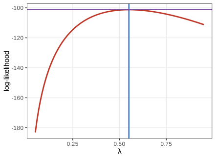
e100 on a grid of 100 values of \(\lambda\) (red), with the sample mean \(\bar x=0.55\) (blue) and \(\ell(\bar x)\) (purple). The maximum is at the sample mean, as Result 2.1 proves. Code: fig_2_4. Reproduces Holmes and Huber (2019), Figure 2.4. PDF · SVGThe function goodfit of the package vcd returns the same value, \(\widehat\lambda=0.55\), together with the observed and fitted frequencies (the components observed, count, fitted, type, method, df and par asked about in Question 2.5).
2.3.1 Classical statistics for classical data
Section 2.3.1 For counts \(k_1,\dots,k_{100}\) the log-likelihood of the Poisson model is
\[ \log L(\lambda,x)=\sum_{i=1}^{100}\big(-\lambda+k_i\log\lambda-\log(k_i!)\big)=-100\lambda+\log\lambda\sum_{i=1}^{100}k_i+\const, \tag{2.1} \]and setting its derivative to zero,
\[ \frac{\d}{\d\lambda}\log L=-100+\frac1\lambda\sum_{i=1}^{100}k_i=0\quad\Longrightarrow\quad\lambda=\frac1{100}\sum_{i=1}^{100}k_i=\bar k . \tag{2.2} \]The book stops here. A zero derivative alone does not make a maximum, and an estimate is of little use without a measure of its precision; both are supplied below.
Result 2.1 (the Poisson MLE and its precision) Section 2.3.1, (2.1)–(2.2)
Let \(x_1,\dots,x_n\) be independent \(\Pois(\lambda)\) with \(\lambda>0\), and \(T=\sum_ix_i\). If \(T>0\), the MLE is \(\widehat\lambda=T/n=\bar x\), the unique global maximiser of \(\ell\). It is unbiased with \(\var(\widehat\lambda)=\lambda/n\), the smallest variance any unbiased estimator can have (it attains the Cramér-Rao bound), and \(\sqrt n(\widehat\lambda-\lambda)\) converges in distribution to \(\N(0,\lambda)\). An approximate 95% confidence interval is \(\widehat\lambda\pm1.96\sqrt{\widehat\lambda/n}\).
Filling the gap 2.2: maximum, information and precision of the Poisson MLE Section 2.3.1
This proves Result 2.1 and introduces the Fisher information, which reappears for every model in the chapter.
Proof
Global maximum. From (2.1), \(\ell(\lambda)=-n\lambda+T\log\lambda+\const\) on \((0,\infty)\). Its derivatives are \(\ell'(\lambda)=-n+T/\lambda\) and \(\ell''(\lambda)=-T/\lambda^2\). If \(T>0\) then \(\ell''<0\) everywhere, so \(\ell\) is strictly concave and its unique stationary point \(\lambda=T/n\) is the unique global maximiser (a strictly concave function lies below each of its tangents, and the tangent at a stationary point is horizontal). If \(T=0\) (all counts zero), \(\ell(\lambda)=-n\lambda\) decreases strictly and has no maximiser in \((0,\infty)\); the supremum is approached as \(\lambda\to0\), and if \(\lambda=0\) (the point mass at 0) is admitted, \(\widehat\lambda=0=\bar x\) again.
Sufficiency. The joint probability is \(e^{-n\lambda}\lambda^{T}/\prod_ix_i!\), a function of \(\lambda\) and \(T\) times a function of the data alone. By the factorisation theorem \(T\) is sufficient: the likelihood, and so every likelihood-based conclusion, depends on the data only through \(T\). That is why the book can work from the frequency table instead of the 100 raw values.
Mean and variance. \(T\sim\Pois(n\lambda)\) (a sum of independent Poisson variables is Poisson), so \(\E\widehat\lambda=\lambda\) and \(\var\widehat\lambda=n\lambda/n^2=\lambda/n\).
Fisher information. For one observation, \(\log f(x\given\lambda)=-\lambda+x\log\lambda-\log x!\), with second derivative \(-x/\lambda^2\). The Fisher information is minus its expectation, \(I(\lambda)=\E[X]/\lambda^2=1/\lambda\), and for \(n\) observations \(I_n(\lambda)=n/\lambda\). The Cramér-Rao inequality states that, under regularity conditions that hold here (the support does not depend on \(\lambda\) and differentiation under the sum is allowed), every unbiased estimator \(\tilde\lambda\) has \(\var\tilde\lambda\ge1/I_n(\lambda)=\lambda/n\). The MLE attains this bound, so no unbiased estimator is more precise.
Curvature equals information. The observed information is \(J=-\ell''(\widehat\lambda)=T/\widehat\lambda^2=n/\widehat\lambda\), which is \(I_n\) evaluated at \(\widehat\lambda\). Near its peak, \(\ell(\lambda)\approx\ell(\widehat\lambda)-\tfrac12J(\lambda-\widehat\lambda)^2\): a sharply curved log-likelihood (large \(J\)) pins \(\lambda\) down, a flat one does not.
Asymptotic normality and interval. \(\widehat\lambda\) is an average of independent variables with variance \(\lambda\), so by the central limit theorem \(\sqrt n(\widehat\lambda-\lambda)\to\N(0,\lambda)\). Replacing \(\lambda\) by the consistent \(\widehat\lambda\) in the standard error (Slutsky's lemma) gives the Wald interval \(\widehat\lambda\pm1.96\sqrt{\widehat\lambda/n}\).
Numbers for e100. \(T=55\), \(\widehat\lambda=0.55\), \(J=100/0.55=181.8\) (a finite-difference second derivative of \(\ell\) agrees to \(4\times10^{-5}\)), standard error \(0.074\), and 95% interval \([0.405,0.695]\). A simulation of 20,000 samples of size 100 from \(\Pois(0.55)\) gives \(\var\widehat\lambda=0.00544\) against \(\lambda/n=0.0055\). ∎
Leaving the outlier in is conservative. With the value 7 included, \(\widehat\lambda=0.55\) instead of \(48/99=0.485\). A larger \(\lambda\) makes large maxima more probable under the null model and so gives a larger p-value. Redoing the computation of Chapter 1 with \(\lambda=0.55\) (the book's Task): \(\Prob(X\ge7)=1.87\times10^{-6}\) and \(\Prob(\max_{i\le100}X_i\ge7)\)
Filling the gap 2.3: chi-square and likelihood-ratio tests of a fitted distribution Sections 2.3 and 2.10, goodfit
The book uses goodfit and its likelihood-ratio statistic (Section 2.10) without saying what it computes or where its degrees of freedom come from.
Derivation
The statistics. Group the values into cells \(k=0,1,\dots,K-1\) with observed counts \(O_k\) and fitted counts \(E_k=n\,\pi_k(\widehat\lambda)\), where \(\pi_k(\lambda)\) is the model probability of cell \(k\) (the last cell should collect the tail \(\{k\ge K-1\}\) so that the \(\pi_k\) sum to one). Two statistics measure the discrepancy:
\[ X^2=\sum_k\frac{(O_k-E_k)^2}{E_k}\ \ \text{(Pearson)},\qquad G^2=2\sum_kO_k\log\frac{O_k}{E_k}\ \ \text{(likelihood ratio, or deviance)}, \]with the convention \(0\log0=0\). \(G^2\) is twice the log of the ratio between the multinomial likelihood with free cell probabilities (maximised at \(O_k/n\), Result 2.3) and with probabilities \(\pi_k(\widehat\lambda)\).
The two agree asymptotically. Write \(O_k=E_k+\delta_k\). With \(\sum_kO_k=\sum_kE_k=n\), \(\sum_k\delta_k=0\). Expanding \(\log(1+u)=u-u^2/2+O(u^3)\) with \(u=\delta_k/E_k\),
\[ O_k\log\frac{O_k}{E_k}=(E_k+\delta_k)\Big(\frac{\delta_k}{E_k}-\frac{\delta_k^2}{2E_k^2}+\dots\Big)=\delta_k+\frac{\delta_k^2}{2E_k}+O\Big(\frac{\delta_k^3}{E_k^2}\Big). \]Summing and doubling, \(G^2=X^2+O_p(n^{-1/2})\), because \(\delta_k\) is of order \(\sqrt n\) and \(E_k\) of order \(n\).
Degrees of freedom. With \(K\) cells and a model with \(d\) parameters estimated from the cell counts by maximum likelihood, both statistics converge to \(\chi^2_{K-1-d}\) under the model (Result 2.4 and Filling the gap 2.8 prove the cases used in this chapter). For a Poisson fit \(d=1\), so \(K-2\) degrees of freedom. (If \(\lambda\) is estimated from the raw values, \(\bar x\), rather than from the grouped counts, the limit lies between \(\chi^2_{K-2}\) and \(\chi^2_{K-1}\), a result of Chernoff and Lehmann (1954); the \(K-2\) reference is then slightly liberal.)
What goodfit does. It uses the cells \(0,\dots,\max x\) without a tail cell, sums \(G^2\) over the non-empty cells, and sets the degrees of freedom to (number of non-empty cells) \(-\,2\). For the Shine-Dalgarno counts of Section 2.10 (cells 0–4, all non-empty) this gives \(G^2=4.135\) on 3 degrees of freedom, \(p=0.25\): no evidence against the Poisson model. The course function pois_gof reproduces these numbers exactly.
The epitope data. For e100, \(G^2=19.53\) (on 2 degrees of freedom by goodfit's rule), and 17.31 of it comes from the single cell \(k=7\), where \(E_7=100\,\Prob(X=7)\approx3\times10^{-4}\). Expected counts this small make the chi-square approximation unreliable, so the course code also computes a parametric bootstrap p-value: simulate 2000 samples of size 100 from \(\Pois(0.55)\), refit, recompute \(G^2\); only 0.05% of them reach 19.53. The outlier alone is enough to reject the Poisson model for all 100 positions, while e99 fits well (\(G^2=3.41\), \(p=0.065\) on one degree of freedom). ∎
e100 and e99 and watch the bar for \(k=7\) and the \(G^2\) statistic.Why a known distribution is useful (Question 2.6). A parametric model compresses the data into a few numbers, and once it is trusted it answers questions the data cannot answer directly, such as the probability of rare events far in the tail. It also opens the door to regression: the Poisson or negative binomial mean can be made to depend on covariates, which leads to the generalised linear models of Chapter 8.
2.4 Binomial distributions and maximum likelihood
Section 2.4 A binomial distribution \(\Bin(n,p)\) has two parameters: the number of trials \(n\), usually fixed by the design, and the success probability \(p\), usually unknown.
2.4.1 An example
Section 2.4.1 In a sample of \(n=120\) males, 10 are red-green colour blind. The natural guess \(\widehat p=10/120=1/12\) is the MLE (Result 2.2). Plotting the likelihood on a grid of step 0.005 puts the maximum at 0.085, the grid point nearest to \(0.0833\); a numerical optimiser (optimize) returns \(1/12\) to ten digits.
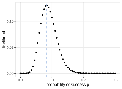
fig_2_5. Reproduces Holmes and Huber (2019), Figure 2.5. PDF · SVG2.4.2 Likelihood for the binomial distribution
Section 2.4.2 For \(y\) successes in \(n\) trials the likelihood and log-likelihood are
\[ f(p\given n,y)=f(y\given n,p)=\binom ny p^y(1-p)^{n-y}, \tag{2.3} \] \[ \log f(p\given y)=\log\binom ny+y\log p+(n-y)\log(1-p). \tag{2.4} \]The same formula is a probability distribution over \(y\) for fixed \(p\), and a likelihood over \(p\) for fixed \(y\). The binomial coefficient does not involve \(p\) and can be dropped (for \(n=300\), \(y=40\) it is about \(9.8\times10^{49}\); lchoose computes its logarithm safely).
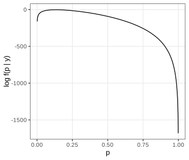
fig_2_6. Reproduces Holmes and Huber (2019), Figure 2.6. PDF · SVGResult 2.2 (binomial MLE, information and intervals) Sections 2.4.1–2.4.2
For \(0<y<n\) the MLE is \(\widehat p=y/n\), the unique global maximiser of (2.4). The Fisher information is \(I_n(p)=n/\{p(1-p)\}\), so \(\se(\widehat p)\approx\sqrt{\widehat p(1-\widehat p)/n}\). Two approximate 95% intervals are the Wald interval \(\widehat p\pm1.96\,\se(\widehat p)\) and the likelihood-ratio interval \(\{p:2[\ell(\widehat p)-\ell(p)]\le3.84\}\), where \(3.84\) is the 95% quantile of \(\chi^2_1\).
Filling the gap 2.4: how flat is "quite flat"? Section 2.4.2, Figure 2.6
The book remarks that "other values of \(p\) are almost equally likely, as the function is quite flat around the maximum". The curvature of the log-likelihood makes this precise.
Derivation
Maximum. \(\ell'(p)=y/p-(n-y)/(1-p)=(y-np)/\{p(1-p)\}\), which is zero only at \(p=y/n\). \(\ell''(p)=-y/p^2-(n-y)/(1-p)^2<0\) for \(0<y<n\), so \(\ell\) is strictly concave and \(y/n\) is the unique global maximiser. (If \(y=0\), \(\ell(p)=(n)\log(1-p)\) is decreasing and the MLE is \(\widehat p=0\); symmetrically \(\widehat p=1\) if \(y=n\).)
Information. For one Bernoulli trial \(\log f=x\log p+(1-x)\log(1-p)\), whose second derivative has expectation \(-p/p^2-(1-p)/(1-p)^2=-1/\{p(1-p)\}\); so \(I_n(p)=n/\{p(1-p)\}\). At the MLE the observed information is the same: \(J=-\ell''(\widehat p)=n\widehat p/\widehat p^2+n(1-\widehat p)/(1-\widehat p)^2=n/\{\widehat p(1-\widehat p)\}\). And \(\var\widehat p=p(1-p)/n=1/I_n(p)\): the Cramér-Rao bound is attained, as for the Poisson.
Quantifying flatness. For \(n=300\), \(y=40\): \(J=300/(0.1333\times0.8667)=2596\), so \(\se(\widehat p)=1/\sqrt J=0.0196\). By the quadratic approximation \(\ell(p)\approx\ell(\widehat p)-\tfrac12J(p-\widehat p)^2\), every \(p\) within one standard error of \(0.133\) has a log-likelihood within \(0.5\) of the maximum, a likelihood ratio of at most \(e^{0.5}=1.65\). On the scale of Figure 2.6 (which spans 1500 log units) that range is invisible: "flat" means "flat relative to the plotted range".
Wilks' theorem and the likelihood-ratio interval. Under \(p=p_0\), a second-order expansion of \(\ell\) at \(\widehat p\) gives \(2[\ell(\widehat p)-\ell(p_0)]\approx J(\widehat p-p_0)^2\), and \(\sqrt J(\widehat p-p_0)\to\N(0,1)\) by the central limit theorem (with \(J/I_n(p_0)\to1\)), so \(2[\ell(\widehat p)-\ell(p_0)]\to\chi^2_1\). Inverting this test gives the likelihood-ratio interval. For 40 of 300:
| 95% interval for \(p\) | lower | upper |
|---|---|---|
| Wald, \(\widehat p\pm1.96\,\se\) | 0.09487 | 0.17180 |
| Likelihood ratio, \(2[\ell(\widehat p)-\ell(p)]\le3.84\) | 0.09804 | 0.17486 |
The likelihood-ratio interval is asymmetric, shifted away from 0, because \(\ell\) falls more steeply towards \(p=0\) than towards \(p=1\) (the term \(y\log p\) with small \(p\)); the Wald interval forces symmetry. A simulation of 20,000 binomial samples with \(p=2/15\) gives the Wald interval a coverage of 94.7%. ∎
Maximum likelihood is one estimation principle among several; others (method of moments, minimum chi-square, Bayesian posterior summaries, Section 2.9) give other hatted quantities. And maximum-likelihood estimates are not always this intuitive: Exercise 2.2 gives one that is biased and does not follow the usual \(1/\sqrt n\) rule.
2.5 More boxes: multinomial data
2.5.1 DNA count modeling: base pairs
Section 2.5.1 DNA is written in four letters: the purines A (adenine) and G (guanine) and the pyrimidines C (cytosine) and T (thymine). A binomial model suffices for the purine/pyrimidine split; for the four letters one needs the multinomial distribution of Chapter 1: \(n\) independent draws, each falling in category \(k\) with probability \(p_k\), \(\sum_kp_k=1\), and the vector of counts \((n_1,\dots,n_K)\sim\Mult(n,\bm p)\) with
\[ \Prob(n_1,\dots,n_K)=\frac{n!}{n_1!\cdots n_K!}\,p_1^{n_1}\cdots p_K^{n_K}. \]Result 2.3 (the multinomial MLE is the vector of observed frequencies) Sections 2.5, 2.7.2
For counts \((n_1,\dots,n_K)\) from \(\Mult(n,\bm p)\) with \(\bm p\) ranging over the probability simplex, the MLE is \(\widehat p_k=n_k/n\). The counts have \(\E n_k=np_k\), \(\var n_k=np_k(1-p_k)\) and \(\cov(n_j,n_k)=-np_jp_k\) for \(j\ne k\).
Filling the gap 2.5: maximising over the simplex Section 2.5
The book uses observed proportions as estimates throughout. Here is why they are the MLE, by two arguments: a Lagrange multiplier (which shows the method) and Gibbs' inequality (which is shorter and handles zero counts).
Proof
Lagrange multiplier. Up to a constant, \(\ell(\bm p)=\sum_kn_k\log p_k\), to be maximised subject to \(\sum_kp_k=1\). Suppose all \(n_k>0\) (a maximiser then has all \(p_k>0\), since \(\ell=-\infty\) otherwise). Stationarity of \(\ell(\bm p)-\mu(\sum_kp_k-1)\) gives \(n_k/p_k=\mu\) for all \(k\), so \(p_k=n_k/\mu\); summing over \(k\), \(\mu=n\). The function \(\ell\) is concave (a sum of concave functions) and the constraint set is convex, so this stationary point is the global maximum.
Gibbs' inequality. Let \(\widehat p_k=n_k/n\) and take any \(\bm p\) in the simplex. Then, summing over \(k\) with \(n_k>0\) and using Jensen's inequality for the concave \(\log\),
\[ \ell(\bm p)-\ell(\widehat{\bm p})=n\sum_k\widehat p_k\log\frac{p_k}{\widehat p_k}\le n\log\sum_k\widehat p_k\frac{p_k}{\widehat p_k}=n\log\sum_{k:\,n_k>0}p_k\le n\log1=0, \]with equality only if \(p_k=\widehat p_k\) for all \(k\). This also covers zero counts (their MLE is 0).
Moments. Write the counts as \(n_k=\sum_{i=1}^n\mathbb 1\{J_i=k\}\), where \(J_i\) is the category of draw \(i\). Indicators of the same draw satisfy \(\mathbb 1\{J_i=j\}\mathbb 1\{J_i=k\}=0\) for \(j\ne k\); draws are independent. Hence \(\E n_k=np_k\), \(\var n_k=np_k(1-p_k)\) and \(\cov(n_j,n_k)=n(0-p_jp_k)=-np_jp_k\): the counts are negatively correlated because they share the fixed total \(n\). ∎
2.5.2 Nucleotide bias
Section 2.5.2 The file staphsequence.ffn.txt holds the coding sequences of 2650 genes of Staphylococcus aureus. The first gene (1362 bases) has counts A 522, C 219, G 229, T 392. Testing it against equal frequencies, as in Chapter 1 (Question 2.9), gives \(X^2=184.4\) on 3 degrees of freedom, \(p\approx10^{-39}\): the letters are far from uniform.
The book then asks whether the first ten genes share one multinomial, without specifying it in advance. It estimates a common vector \(\bm p_0\) as the average of the ten genes' letter proportions, \(\bm p_0=(0.347,0.152,0.201,0.300)\) for (A, C, G, T), forms the expected table \(E_{kg}=p_{0k}\,n_g\) (\(n_g\) the length of gene \(g\)), and computes
\[ S_1=\sum_{g=1}^{10}\sum_{k\in\{\tA,\tC,\tG,\tT\}}\frac{(O_{kg}-E_{kg})^2}{E_{kg}}=70.08 . \]To judge \(S_1\), it simulates 1000 tables with the same gene lengths from \(\Mult(n_g,\bm p_0)\) and recomputes the statistic. None of the 1000 reaches 70.08.
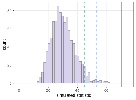
fig_2_7, seed 2. Reproduces Holmes and Huber (2019), Figure 2.7. PDF · SVG2.6 The \(\chi^2\) distribution
Section 2.6 A Monte Carlo p-value from \(B\) simulations cannot go below \(1/B\) and is itself noisy, so a theoretical null distribution is valuable. The book states that simulstat follows a \(\chi^2\) distribution with \(30=10\times(4-1)\) degrees of freedom. Note the double meaning of "chi-square": the statistic \(\sum(O-E)^2/E\) and the distribution below.
Definition 2.3 (the chi-square distribution) Section 2.6
If \(Z_1,\dots,Z_\nu\) are independent \(\N(0,1)\), the law of \(Z_1^2+\dots+Z_\nu^2\) is the chi-square distribution with \(\nu\) degrees of freedom, \(\chi^2_\nu\). It has density \(x^{\nu/2-1}e^{-x/2}/\{2^{\nu/2}\Gamma(\nu/2)\}\) on \(x>0\), mean \(\nu\) and variance \(2\nu\).
Result 2.4 (Pearson's statistic is asymptotically chi-square) Section 2.6
Let \((N_1,\dots,N_K)\sim\Mult(n,\bm\pi)\) with all \(\pi_k>0\) known. Then, as \(n\to\infty\),
\[ X^2=\sum_{k=1}^K\frac{(N_k-n\pi_k)^2}{n\pi_k}\ \xrightarrow{d}\ \chi^2_{K-1}. \]For \(G\) independent multinomials (one per gene) with known probabilities, the statistics add and the limit is \(\chi^2_{G(K-1)}\); for the ten genes and four letters, \(\chi^2_{30}\).
Filling the gap 2.6: proof of Pearson's theorem Section 2.6
The book asserts the \(\chi^2\) law and checks it by a QQ plot. The proof needs only the multivariate central limit theorem and one fact about projections.
Proof
Step 1: a multivariate CLT. Write \(\bm N=\sum_{i=1}^n\bm e_{J_i}\), where \(\bm e_{J_i}\) is the indicator vector of the category of draw \(i\). These vectors are independent with mean \(\bm\pi\) and covariance \(\diag(\bm\pi)-\bm\pi\bm\pi^\T\) (Result 2.3). By the multivariate central limit theorem, \((\bm N-n\bm\pi)/\sqrt n\to\N_K(\bm0,\diag(\bm\pi)-\bm\pi\bm\pi^\T)\).
Step 2: standardise. Let \(Z_k=(N_k-n\pi_k)/\sqrt{n\pi_k}\), i.e. \(\bm Z=D^{-1/2}(\bm N-n\bm\pi)/\sqrt n\) with \(D=\diag(\bm\pi)\). By Step 1, \(\bm Z\to\N_K(\bm0,\Sigma)\) with
\[ \Sigma=D^{-1/2}\big(D-\bm\pi\bm\pi^\T\big)D^{-1/2}=I-\bm u\bm u^\T,\qquad \bm u=\big(\sqrt{\pi_1},\dots,\sqrt{\pi_K}\big)^\T. \]Step 3: \(\Sigma\) is a projection of rank \(K-1\). Since \(\bm u^\T\bm u=\sum_k\pi_k=1\), \(\Sigma^2=I-2\bm u\bm u^\T+\bm u(\bm u^\T\bm u)\bm u^\T=\Sigma\), and \(\Sigma\) is symmetric: it is the orthogonal projection onto the hyperplane \(\bm u^\perp\), of dimension \(K-1\) (its trace is \(K-1\)). Its eigenvalues for the ten-gene \(\bm p_0\) are exactly \(1,1,1,0\).
Step 4: the squared length of a projected Gaussian. Choose an orthonormal basis \(\bm v_1,\dots,\bm v_{K-1}\) of \(\bm u^\perp\) and let \(V\) be the \(K\times(K-1)\) matrix with these columns, so \(\Sigma=VV^\T\). If \(\bm W\sim\N_{K-1}(\bm0,I)\), then \(V\bm W\sim\N_K(\bm0,VV^\T)=\N_K(\bm0,\Sigma)\) and \(\|V\bm W\|^2=\bm W^\T V^\T V\bm W=\|\bm W\|^2\sim\chi^2_{K-1}\).
Step 5: conclude. \(X^2=\|\bm Z\|^2\) is a continuous function of \(\bm Z\), so by the continuous mapping theorem \(X^2\to\|V\bm W\|^2\sim\chi^2_{K-1}\). One degree of freedom is lost because the \(K\) residuals satisfy one linear constraint, \(\sum_k\sqrt{\pi_k}Z_k=0\). For \(G\) independent multinomials the \(G\) statistics are independent, and a sum of independent \(\chi^2_{K-1}\) variables is \(\chi^2_{G(K-1)}\). ∎
Accuracy. The limit is a good guide when all expected counts are at least about 5. In the ten-gene table the smallest expected count is 37, so the approximation is excellent; the 1000 simulated values have mean 30.5 (theory 30).
2.6.1 Intermezzo: quantiles and the quantile-quantile plot
Section 2.6.1 A histogram compares distributions poorly; comparing their quantiles is sharper.
Definition 2.4 (quantiles, sample quantiles) Section 2.6.1
The quantile function of a distribution function \(F\) is \(Q(u)=\inf\{x:F(x)\ge u\}\) for \(0<u<1\); \(Q(0.5)\) is the median (Question 2.11). For a sample with order statistics \(x_{(1)}\le\dots\le x_{(n)}\) and empirical distribution function \(\widehat F_n(x)=\#\{i:x_i\le x\}/n\), any \(c\) with \(x_{(\lceil nu\rceil)}\le c\), roughly where \(\widehat F_n\) crosses \(u\), is a \(u\)-quantile; the book's \(c_{0.22}\) lies between \(x_{(22)}\) and \(x_{(23)}\). Software must pick one value: R's default (quantile(type = 7), Question 2.12) interpolates linearly between \(x_{(j)}\) and \(x_{(j+1)}\) at position \(h=(n-1)u+1\), \(j=\lfloor h\rfloor\); eight other conventions are available through the argument type.
Filling the gap 2.7: why a QQ plot should be a straight line Section 2.6.1, Figure 2.8
Derivation
A QQ plot of a sample against a distribution \(F\) plots \(x_{(i)}\) against \(Q(u_i)\) for "plotting positions" \(u_i\) spread over \((0,1)\). R's ppoints(n) uses \(u_i=(i-a)/(n+1-2a)\) with \(a=3/8\) for \(n\le10\) and \(a=1/2\) otherwise, the midpoints \((i-1/2)/n\) of \(n\) equal slices of \((0,1)\).
Why it works. If the sample comes from a continuous \(F\), the values \(U_{(i)}=F(x_{(i)})\) are the order statistics of a uniform sample, with \(\E U_{(i)}=i/(n+1)\approx u_i\). So \(x_{(i)}=Q(U_{(i)})\approx Q(u_i)\): the points lie near the identity line, with scatter that is small in the middle and larger in the tails (where \(Q\) is steep).
Location and scale. If instead the sample comes from \(X=\mu+\sigma Y\) with \(Y\sim F\), then \(x_{(i)}\approx\mu+\sigma Q(u_i)\): the points still lie on a straight line, of slope \(\sigma\) and intercept \(\mu\). A QQ plot therefore checks the shape of a distribution independently of its location and scale; curvature means a different shape (heavier or lighter tails, skewness). ∎
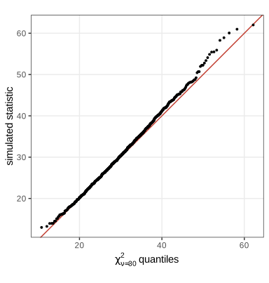
ppoints(1000), with the identity line. The points follow the line, with the usual extra scatter in the upper tail. Code: fig_2_8. Reproduces Holmes and Huber (2019), Figure 2.8. PDF · SVGThe book concludes with \(\Prob(\chi^2_{30}\ge70.08)=4.7\times10^{-5}\). The simulated values do follow \(\chi^2_{30}\), but the observed \(S_1\) should not be referred to that distribution, because \(\bm p_0\) was estimated from the same ten genes.
Filling the gap 2.8: estimated probabilities cost degrees of freedom (27, not 30) Sections 2.5.2 and 2.6
In the simulation \(\bm p_0\) is held fixed, so the simulated statistics are \(\chi^2_{30}\) (Result 2.4) and Figure 2.8 is correct. But for the real table \(\bm p_0\) was fitted to the same data, which pulls the expected counts towards the observed ones and makes the statistic smaller than it would be with the true \(\bm p\).
Derivation
The test of homogeneity. The hypothesis is that the \(G=10\) genes share one unknown \(\bm p\) (\(K-1=3\) free parameters). Its MLE pools the genes: the likelihood is \(\prod_g\prod_kp_k^{O_{kg}}=\prod_kp_k^{O_{k\cdot}}\) with \(O_{k\cdot}=\sum_gO_{kg}\), a single multinomial likelihood, so by Result 2.3 \(\widehat p_k=O_{k\cdot}/O_{\cdot\cdot}\). (The book's \(\bm p_0\), an unweighted mean of the ten genes' proportions, gives each gene the same weight regardless of length; it is close to, but not, the MLE.)
Counting degrees of freedom. Under the general alternative each gene has its own \(\bm p_g\): \(G(K-1)=30\) free parameters. Under homogeneity there are \(K-1=3\). The general theorem behind Filling the gap 2.3 (Pearson's statistic with parameters estimated by maximum likelihood from the same counts) says that the limit is chi-square with the difference, \(30-3=27=(G-1)(K-1)\) degrees of freedom. The geometric reason extends Step 3 of Filling the gap 2.6: fitting \(d\) parameters by maximum likelihood makes the standardised residuals orthogonal to a further \(d\)-dimensional subspace (the directions in which the fitted model can move), so their limiting covariance is a projection of rank \(G(K-1)-d\).
Simulation. We redo the book's simulation but re-estimate \(\bm p\) (pooled MLE) in every simulated table, as the analysis of real data does. The mean of 2000 statistics is 26.8, matching \(\chi^2_{27}\) (mean 27), not \(\chi^2_{30}\) (mean 30); with \(\bm p_0\) fixed the mean is 30.5.
The corrected p-value. With the pooled MLE the statistic is \(68.65\), exactly R's chisq.test(tab10), and \(\Prob(\chi^2_{27}\ge68.65)=1.7\times10^{-5}\). The book's value \(4.7\times10^{-5}\) is about three times too large, so the conclusion (the ten genes do not share one composition) only becomes stronger. ∎
2.7 Chargaff's rule
Section 2.7 Before sequencing, Chargaff measured the mass percentages of the four bases in the DNA of several organisms (Elson and Chargaff, 1952). His data reject the "tetranucleotide hypothesis" of equal proportions (Question 2.13: M. tuberculosis, for example, has 15% A and 35% C) and show a different regularity: the percentage of A matches that of T, and that of C matches G, while the A+T versus C+G balance varies from organism to organism.
| Organism | A | T | C | G |
|---|---|---|---|---|
| Human thymus | 30.9 | 29.4 | 19.9 | 19.8 |
| M. tuberculosis | 15.1 | 14.6 | 34.9 | 35.4 |
| Chicken erythrocytes | 28.8 | 29.2 | 20.5 | 21.5 |
| Sheep liver | 29.3 | 29.3 | 20.5 | 20.7 |
| Sea urchin | 32.8 | 32.1 | 17.7 | 17.3 |
| Wheat | 27.3 | 27.1 | 22.7 | 22.8 |
| Yeast | 31.3 | 32.9 | 18.7 | 17.1 |
| E. coli | 24.7 | 23.6 | 26.0 | 25.7 |
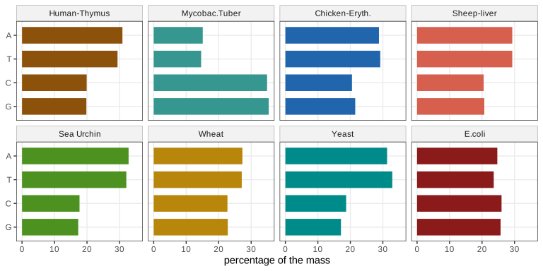
fig_2_9. Reproduces Holmes and Huber (2019), Figure 2.9. PDF · SVGTo test the pattern, the book uses the statistic \(S=\sum_{\text{rows}}\big[(p_\tC-p_\tG)^2+(p_\tA-p_\tT)^2\big]\), which is small when the pairing holds; for the table, \(S=11.1\). Under the null hypothesis the four values in each row carry no particular relationship to the labels, so the book permutes each row at random 100,000 times and reports the fraction of permuted tables with \(S\le11.1\), \(p=0.00019\).
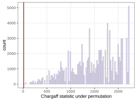
fig_2_10. Reproduces Holmes and Huber (2019), Figure 2.10. PDF · SVGFilling the gap 2.9: the permutation test, its validity and its exact p-value Section 2.7, Question 2.14
The book runs 100,000 random permutations. The test can be justified in a few lines, and for this table its p-value can be computed exactly by enumeration.
Derivation
Null hypothesis. \(H_0\): within each row, the assignment of the four observed values to the labels A, T, C, G is uniformly random over the \(4!=24\) orderings, independently across rows ("exchangeability"). Under \(H_0\) the observed table is a uniform draw from the set \(\mathcal O\) of \(24^8\) tables obtained by permuting each row; this set (the orbit) does not depend on which member was observed.
Validity. Let \(s_1\le\dots\le s_M\) be the values of \(S\) over the orbit (\(M=|\mathcal O|\)) and define the p-value \(p(t)=\#\{j:s_j\le S(t)\}/M\) for a table \(t\). For any \(\alpha\), let \(s^*\) be the largest orbit value with \(\#\{j:s_j\le s^*\}\le\alpha M\). Then \(p(t)\le\alpha\) exactly when \(S(t)\le s^*\), and under \(H_0\), \(\Prob(p\le\alpha)=\#\{j:s_j\le s^*\}/M\le\alpha\). So the test has level \(\alpha\) for every \(\alpha\), without any distributional assumption beyond exchangeability. This matters here because the data are percentages of mass, not counts, so no multinomial model is available.
Reduction to \(3^8\) cases. For one row with values \((a,b,c,d)\) assigned to (A, T, C, G), \(S_{\text{row}}=(a-b)^2+(c-d)^2\) depends only on how the four values are split into the pair placed on {A, T} and the pair placed on {C, G}. There are three such splittings of four values into two pairs: \(\{ab|cd\}\), \(\{ac|bd\}\), \(\{ad|bc\}\). Each is produced by \(24/3=8\) orderings (2 orders within each pair, 2 ways to assign the pairs to {A,T} and {C,G}), which listing all 24 confirms. So under \(H_0\), \(S\) is a sum of 8 independent variables, each uniform on three values, and its exact distribution consists of \(3^8=6561\) equally likely totals.
Exact p-value. Enumerating the 6561 totals, only the observed pairing in every row gives \(S\le11.1\): the exact p-value is \(1/6561=0.000152\). Random permutation estimates it with Monte Carlo error: the book's 0.00019 and the course's 0.00010 (seed 3) are both within about two standard errors \(\sqrt{p(1-p)/10^5}=0.00004\) of it. In general a Monte Carlo p-value should be reported as \((1+b)/(1+B)\), where \(b\) of \(B\) permutations are at least as extreme; this version is itself a valid p-value, since the observed table counts as one of the permutations.
One-sided (Question 2.14). The alternative of interest is base pairing, which predicts small differences \(p_\tA-p_\tT\) and \(p_\tC-p_\tG\). Large values of \(S\) would mean the pairs are more different than random relabelling makes them, which is evidence for nothing Chargaff proposed; so only the lower tail counts as extreme. ∎
2.7.1 Two categorical variables
Section 2.7.1 When two categorical variables are recorded on each subject, the cross-tabulated counts form a contingency table. R's HairEyeColor is a three-way table (Question 2.15): a numeric array of dimension \(4\times4\times2\) (hair, eye, sex) with class table.
Colour blindness and sex. In a survey of 2000 men and 2000 women, 19 men and 2 women had deuteranopia. The book applies chisq.test and reports \(X^2=12.255\), \(p=0.00046\).
| Men | Women | Total | |
|---|---|---|---|
| Deuteranope | 19 | 2 | 21 |
| Not deuteranope | 1981 | 1998 | 3979 |
| Total | 2000 | 2000 | 4000 |
Filling the gap 2.10: the chi-square test of independence and Yates' correction Section 2.7.1
The book says the null model consists of "two independent binomials" and lets chisq.test do the rest. What is estimated, and why one degree of freedom?
Derivation
Expected counts are MLEs. Model the \(r\times c\) table as one multinomial with cell probabilities \(\pi_{ij}\). Independence means \(\pi_{ij}=a_ib_j\) with \(\sum_ia_i=\sum_jb_j=1\). The likelihood \(\prod_{ij}(a_ib_j)^{n_{ij}}=\prod_ia_i^{n_{i+}}\prod_jb_j^{n_{+j}}\) factorises into two multinomial likelihoods, so by Result 2.3 \(\widehat a_i=n_{i+}/n\), \(\widehat b_j=n_{+j}/n\), and the fitted counts are \(E_{ij}=n_{i+}n_{+j}/n\).
Degrees of freedom. The full model has \(rc-1\) free probabilities, the independence model \((r-1)+(c-1)\); the difference is \((r-1)(c-1)\), which is 1 for a \(2\times2\) table. The same statistic and degrees of freedom arise if the column totals were fixed by design (2000 men and 2000 women sampled separately, two binomials compared for equal deuteranopia rates): the likelihood then factorises by column and the fitted counts are the same.
A closed form for \(2\times2\) tables. With cells \(a,b\) (first row), \(c,d\) (second row), every cell has the same absolute residual \(|O-E|=|ad-bc|/n\) (the residuals of a \(2\times2\) table are \(\pm\) one number because rows and columns sum to zero). Summing \((O-E)^2/E\) over the four cells and simplifying \(\sum1/E_{ij}=n^3/(n_{1+}n_{2+}n_{+1}n_{+2})\),
\[ X^2=\frac{n(ad-bc)^2}{n_{1+}n_{2+}n_{+1}n_{+2}},\qquad X^2_{\text{Yates}}=\sum_{ij}\frac{(|O_{ij}-E_{ij}|-\tfrac12)^2}{E_{ij}}=\frac{n(|ad-bc|-n/2)^2}{n_{1+}n_{2+}n_{+1}n_{+2}}. \]For the table: \(ad-bc=19\cdot1998-2\cdot1981=34000\), so \(X^2=4000\cdot34000^2/(21\cdot3979\cdot2000\cdot2000)=13.835\) and the Yates version, which chisq.test uses by default for \(2\times2\) tables, is \(4000\cdot32000^2/(\dots)=12.255\). Yates' correction subtracts \(1/2\) from each \(|O-E|\) to make the discrete statistic's upper tail closer to the continuous \(\chi^2_1\); it is conservative. The smallest expected count, \(21\cdot2000/4000=10.5\), is large enough for the approximation, and Fisher's exact test (Section 10.3.2 of the book) confirms the result. ∎
2.7.2 A special multinomial: Hardy-Weinberg equilibrium
Section 2.7.2 A gene with two alleles M and N, with population frequencies \(p\) and \(q=1-p\), produces three genotypes. If the two alleles a person carries are drawn independently (random mating in a large population with no selection, among other conditions), the genotype probabilities are
\[ p_{\text{MM}}=p^2,\qquad p_{\text{NN}}=q^2,\qquad p_{\text{MN}}=2pq, \tag{2.5} \]the Hardy-Weinberg equilibrium (HWE; Hardy, 1908). Given genotype counts \((n_{\text{MM}},n_{\text{MN}},n_{\text{NN}})\) with total \(S\), the log-likelihood under HWE is, up to a constant,
\[ L(p)=n_{\text{MM}}\log(p^2)+n_{\text{MN}}\log(2pq)+n_{\text{NN}}\log(q^2). \]Result 2.5 (Hardy-Weinberg MLE and test) Section 2.7.2
The MLE of the allele frequency is the allele-counting estimate \(\widehat p=(2n_{\text{MM}}+n_{\text{MN}})/(2S)\), with \(\var\widehat p=pq/(2S)\) under HWE. The Pearson statistic for HWE has 1 degree of freedom and equals
\[ X^2=\frac{S\,(4n_{\text{MM}}n_{\text{NN}}-n_{\text{MN}}^2)^2}{(2n_{\text{MM}}+n_{\text{MN}})^2(2n_{\text{NN}}+n_{\text{MN}})^2}. \]Filling the gap 2.11: the Hardy-Weinberg likelihood, its maximum and the test Section 2.7.2 (the book refers to Rice, 2006)
Proof
Gene counting. Collect the powers of \(p\) and \(q\): \(L(p)=(2n_{\text{MM}}+n_{\text{MN}})\log p+(n_{\text{MN}}+2n_{\text{NN}})\log(1-p)+n_{\text{MN}}\log2\). Writing \(A=2n_{\text{MM}}+n_{\text{MN}}\) (the number of M alleles among the \(2S\) sampled) and \(B=2S-A\), this is the binomial log-likelihood (2.4) for \(A\) successes in \(2S\) trials, so by Result 2.2 \(\widehat p=A/(2S)\), the unique maximum because \(L''(p)=-A/p^2-B/q^2<0\).
Precision. Under HWE the \(2S\) alleles are independent draws, so \(A\sim\Bin(2S,p)\) exactly and \(\var\widehat p=pq/(2S)\); the Fisher information is \(2S/(pq)\). For Tahiti (\(n_{\text{MM}}=188\), \(n_{\text{MN}}=296\), \(n_{\text{NN}}=96\), \(S=580\)): \(\widehat p=672/1160=0.5793\), standard error 0.0145; 20,000 simulated HWE samples give a variance within 2% of \(pq/(2S)\).
Test. Three cells, one estimated parameter: \(3-1-1=1\) degree of freedom. Write \(a,b,c\) for the three counts. The fitted counts are \(E_{\text{MM}}=A^2/(4S)\), \(E_{\text{MN}}=AB/(2S)\), \(E_{\text{NN}}=B^2/(4S)\). Expanding, \(4Sa-A^2=4a(a+b+c)-(2a+b)^2=4ac-b^2=:\Delta\), so the residual in cell MM is \(\Delta/(4S)\); by the same algebra it is \(\Delta/(4S)\) in cell NN, and \(-\Delta/(2S)\) in cell MN (residuals sum to 0). Then
\[ X^2=\frac{\Delta^2}{16S^2}\Big(\frac{4S}{A^2}+\frac{4S}{B^2}\Big)+\frac{\Delta^2}{4S^2}\cdot\frac{2S}{AB}=\frac{\Delta^2}{4S}\Big(\frac1A+\frac1B\Big)^2=\frac{\Delta^2}{4S}\cdot\frac{(2S)^2}{A^2B^2}=\frac{S\Delta^2}{A^2B^2}. \]This closed form agrees with HardyWeinberg::HWChisq (without continuity correction). For Tahiti the expected counts are 194.6, 282.7, 102.6 and \(X^2=1.28\), \(p=0.26\): no evidence against HWE. ∎
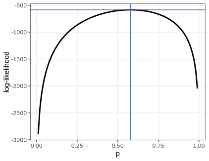
Mourant data of the HardyWeinberg package, after Mourant et al., 1976) on the grid \(0.01,\dots,0.99\), with the maximum \(\widehat p=0.579\) marked. Code: fig_2_11. Reproduces Holmes and Huber (2019), Figure 2.11. PDF · SVGVisual comparison to the Hardy-Weinberg equilibrium
The de Finetti diagram places a population with genotype proportions \((x_{\text{MM}},x_{\text{MN}},x_{\text{NN}})\) inside a triangle whose corners are the three pure genotypes, at the barycentre of the corners weighted by the proportions.
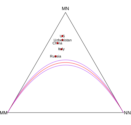
Mourant data (Russia, Italy, Uzbekistan, China, US), drawn with HWTernaryPlot; red: the HWE curve, purple: the limits of the acceptance region of the chi-square test at \(\alpha=10^{-4}\). All five lie above the region: too many heterozygotes. Code: fig_2_12. Reproduces Holmes and Huber (2019), Figure 2.12. PDF · SVGFilling the gap 2.12: the geometry of the de Finetti diagram Section 2.7.2, Figure 2.12, Questions 2.16–2.17
Derivation
Coordinates. Put MM at \((0,0)\), NN at \((1,0)\) and MN at \((\tfrac12,\tfrac{\sqrt3}2)\). The barycentre is \((u,h)\) with \(u=x_{\text{NN}}+\tfrac12x_{\text{MN}}\) and \(h=\tfrac{\sqrt3}2x_{\text{MN}}\). The horizontal coordinate \(u\) is exactly the frequency \(q\) of allele N (count the N alleles: two per NN, one per MN), whatever the genotype proportions; the height is proportional to the heterozygote proportion.
The HWE curve is a parabola. Under (2.5), \(x_{\text{MN}}=2q(1-q)\), so \(h=\sqrt3\,q(1-q)\): a parabola through MM and NN with apex at \(q=\tfrac12\), half-way up the triangle. Equivalently, HWE holds exactly when \(\delta=4x_{\text{MM}}x_{\text{NN}}-x_{\text{MN}}^2=0\). Points above the parabola have an excess of heterozygotes, points below a deficit.
The acceptance region. In proportions, \(\Delta=S^2\delta\), \(A=2S\widehat p\), \(B=2S\widehat q\), so Result 2.5 reads \(X^2=S\delta^2/(16\widehat p^2\widehat q^2)\). The test accepts when \(X^2\le c=\chi^2_{1,1-\alpha}\) (\(c=15.14\) for \(\alpha=10^{-4}\)), i.e. \(|\delta|\le4\widehat p\widehat q\sqrt{c/S}\): a band around the parabola whose half-width shrinks like \(1/\sqrt S\).
Question 2.17. Dividing all counts by 50 leaves the points (the proportions) where they are but divides \(S\) by 50, so the band widens by \(\sqrt{50}\approx7.1\): with less data, larger departures from HWE are compatible with it. (By default HWTernaryPlot draws the band for the largest sample in the plot, here Russia with \(S=5728\), and with a continuity correction; the two purple curves are its upper and lower limits.)
Which population is furthest from HWE? The book's caption names the US, and geometrically it is the highest point (76% heterozygotes against 50% expected). In evidence, measured by \(X^2\), the order is different: Uzbekistan 258.5, US 175.8, Russia 144.7, China 139.2, Italy 85.2. Uzbekistan has a slightly smaller excess (72% heterozygotes) but twice the sample size (1265 against 619), and \(X^2\) grows linearly in \(S\) for fixed proportions. Distance on the diagram measures effect size; the chi-square statistic measures evidence (Question 2.16 asks for exactly this comparison using HWChisq). ∎
2.7.3 Concatenating several multinomials: sequence motifs and logos
Section 2.7.3 The Kozak motif surrounds the start codon ATG of many eukaryotic genes. A position weight matrix (PWM, or position-specific scoring matrix) gives one multinomial distribution over A, C, G, T for each position; positions are modelled as independent, so a sequence \(x_1\cdots x_9\) has probability \(\prod_jp_j(x_j)\). The Kozak PWM below has columns 6–8 equal to the start codon.
| Position | 1 | 2 | 3 | 4 | 5 | 6 | 7 | 8 | 9 |
|---|---|---|---|---|---|---|---|---|---|
| A | 0.33 | 0.25 | 0.40 | 0.15 | 0.20 | 1 | 0 | 0 | 0.05 |
| C | 0.12 | 0.25 | 0.10 | 0.40 | 0.40 | 0 | 0 | 0 | 0.05 |
| G | 0.33 | 0.25 | 0.40 | 0.20 | 0.25 | 0 | 0 | 1 | 0.90 |
| T | 0.22 | 0.25 | 0.10 | 0.25 | 0.15 | 0 | 1 | 0 | 0.00 |
| Information (bits) | 0.097 | 0.000 | 0.278 | 0.096 | 0.096 | 2 | 2 | 2 | 1.431 |
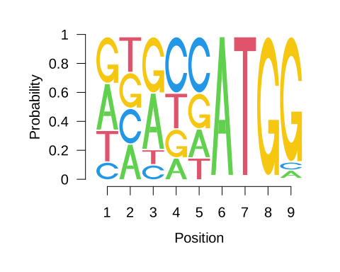
seqLogo(..., ic.scale = FALSE): at each position the letters are stacked with heights equal to their probabilities, largest on top. Code: fig_2_13. Reproduces Holmes and Huber (2019), Figure 2.13. PDF · SVGFilling the gap 2.13: information content of a logo column Section 2.7.3, Figure 2.13
Derivation
For a column with letter probabilities \(\bm p_j\), the entropy \(H_j=-\sum_bp_{jb}\log_2p_{jb}\) (in bits, with \(0\log0=0\)) lies between 0 (one certain letter) and 2 (all four equally likely). The information content is
\[ IC_j=2-H_j=\sum_bp_{jb}\log_2\frac{p_{jb}}{1/4}=\KL\big(\bm p_j\,\|\,\text{uniform}\big)\ge0, \]the Kullback-Leibler divergence from the uniform background, non-negative by Gibbs' inequality (Filling the gap 2.5). In the standard logo of Schneider and Stephens (1990), the stack at position \(j\) has total height \(IC_j\) and letter \(b\) gets height \(p_{jb}IC_j\), so conserved positions stand tall and uninformative ones vanish. The information row of the table above agrees with the ic slot computed by seqLogo (a check).
A remark on Figure 2.13. The book's caption says the logo "codifies the amount of variation in each of the positions on a log scale". That describes the information-scaled logo (ic.scale = TRUE), but the figure is drawn with ic.scale = FALSE, where every column has height 1 and letters are scaled by probability. In the figure position 2 (uniform, 0 bits) is therefore as tall as positions 6–8 (2 bits each); on the information scale it would be empty. ∎
Most real multinomials have unequal category probabilities (amino acids, blood types, hair colour), and pairs of categorical variables are rarely independent (sex and colour blindness, hair and eye colour). The next section models one important kind of dependence: along a sequence.
2.8 Modeling sequential dependencies: Markov chains
Section 2.8 Tomorrow's weather depends mostly on today's, not on last week's. The Markov assumption formalises such a finite memory. Along DNA, adjacent letters are not independent: some dinucleotides (digrams) are more frequent than the product of the single-letter frequencies, \(\Prob(\tC\tA)\ne\Prob(\tC)\Prob(\tA)\).
Definition 2.5 (Markov chain on the four letters) Section 2.8
A sequence of random letters \(X_1,X_2,\dots\) is a (first-order, time-homogeneous) Markov chain with transition matrix \(P\) if \(\Prob(X_t=y\given X_1,\dots,X_{t-1})=P_{X_{t-1}y}\) for every \(t\): the next letter depends on the past only through the current letter. \(P\) is a \(4\times4\) matrix with non-negative entries and rows summing to 1 (row = from, column = to). A distribution \(\bm\pi\) with \(\bm\pi^\T P=\bm\pi^\T\) is stationary: if \(X_1\sim\bm\pi\) then every \(X_t\sim\bm\pi\). A chain of order \(k\) conditions on the previous \(k\) letters instead.
Result 2.6 (likelihood of a sequence and the transition-matrix MLE) Sections 2.8 and 2.10.1
For an observed sequence \(x_1\cdots x_L\) with transition counts \(n_{ij}=\#\{t:x_{t-1}=i,x_t=j\}\),
\[ \Prob(x_1,\dots,x_L)=\Prob(X_1=x_1)\prod_{t=2}^LP_{x_{t-1}x_t}=\Prob(X_1=x_1)\prod_{i,j}P_{ij}^{\,n_{ij}}, \]and the MLE of the transition matrix is \(\widehat P_{ij}=n_{ij}/n_{i+}\), with \(n_{i+}=\sum_jn_{ij}\) the number of transitions out of \(i\). For a stationary chain, the probability of the digram \(xy\) at any position is \(\pi_xP_{xy}\).
Filling the gap 2.14: estimating a transition matrix, and what a digram probability is Section 2.8, Figure 2.14; Section 2.10.1
Proof
Likelihood. By the chain rule of probability, \(\Prob(x_1,\dots,x_L)=\Prob(x_1)\prod_{t\ge2}\Prob(x_t\given x_1,\dots,x_{t-1})\), and the Markov property replaces each factor by \(P_{x_{t-1}x_t}\). Grouping equal factors gives the product over \((i,j)\).
MLE row by row. Treat the initial letter as fixed (or give it its own parameters). The log-likelihood \(\sum_i\sum_jn_{ij}\log P_{ij}\) is a sum over rows \(i\) of terms that involve only row \(i\), and each row is constrained separately (\(\sum_jP_{ij}=1\)). So each row is maximised on its own, and row \(i\) is exactly the multinomial problem of Result 2.3 with counts \((n_{i1},\dots,n_{i4})\): \(\widehat P_{ij}=n_{ij}/n_{i+}\). This agrees with markovchain::markovchainFit and with direct numerical maximisation of a row.
Digram probabilities. \(\Prob(X_t=x,X_{t+1}=y)=\Prob(X_t=x)P_{xy}\), which equals \(\pi_xP_{xy}\) for every \(t\) when the chain is stationary. The book's chain of equalities \(\Prob(\tC\tA)=\Prob(\text{N}\tC\tA)=\dots=\Prob(\tC)\Prob(\tA\given\tC)\) is this statement: it holds when the letter frequencies do not change along the sequence. A simulated stationary chain of length \(2\times10^5\) reproduces \(\pi_xP_{xy}\) within 0.0012.
Independence as a special case. If every row of \(P\) equals \(\bm\pi\), then \(\Prob(xy)=\pi_x\pi_y\) and the letters are independent. Comparing the zero-order model (independence) with the first-order chain is the chi-square test of independence (Filling the gap 2.10) applied to the \(4\times4\) table of transition counts, with \((4-1)^2=9\) degrees of freedom. "Are the rows different?" (Question 2.24) is exactly this test.
Counting across several sequences. When transitions are pooled over many separate sequences (Section 2.10.1), the counts must not include the pair formed by the last letter of one sequence and the first of the next. Summing dinucleotideFrequency over the sequences, as the book does, respects this. ∎
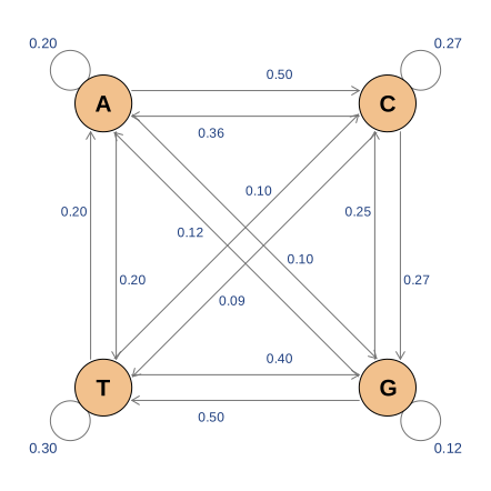
fig_2_14. Reproduces Holmes and Huber (2019), Figure 2.14. PDF · SVG2.9 Bayesian thinking
Section 2.9 So far parameters were fixed unknown constants, estimated from the data alone. The Bayesian approach describes what is known about a parameter before the data by a probability distribution, the prior, and updates it with the data to a posterior. The posterior after one experiment can serve as the prior for the next, which makes the approach natural for combining sources of information. The book's Figure 2.15 (a cartoon of "turtles all the way down") makes the point that the prior's own parameters can be given priors in turn, which leads to hierarchical models; Figures 2.16–2.18 (schematics and a database screenshot about Y-chromosome short tandem repeats) are not reproduced.
Definition 2.6 (prior, posterior, Bayes' theorem) Section 2.9
Let \(\pi(\theta)\) be a prior density on \(\Theta\) and \(f(x\given\theta)\) the model. The posterior is the conditional density of \(\theta\) given the data,
\[ \pi(\theta\given x)=\frac{f(x\given\theta)\,\pi(\theta)}{m(x)},\qquad m(x)=\int_\Theta f(x\given\theta)\,\pi(\theta)\,\d\theta, \]where \(m(x)\) is the marginal (or prior predictive) distribution of the data. In words: posterior \(\propto\) likelihood \(\times\) prior. For a hypothesis \(H\) the same rule turns a prior probability \(\Prob(H)\) into a posterior probability \(\Prob(H\given D)\).
2.9.1 Example: haplotype frequencies
Section 2.9.1 A haplotype is a set of alleles at linked loci on one chromosome, usually inherited together. Y-chromosome haplotypes are defined by the repeat numbers at several short tandem repeat (STR) loci: haplotype H1, for example, has 14 repeats at DYS19, 12 at DXYS156Y, and so on. Forensic work needs the population frequency \(p\) of a haplotype. The running example: \(n=300\) men are typed and \(y=40\) carry H1; model \(Y\sim\Bin(300,p)\) with \(p\) unknown.
2.9.2 Simulation study of the Bayesian paradigm for the binomial distribution
Section 2.9.2 A prior for a proportion should live on \([0,1]\). The Beta family is flexible and, as the book states and Result 2.8 proves, convenient:
\[ f_{\alpha,\beta}(x)=\frac{x^{\alpha-1}(1-x)^{\beta-1}}{\mathrm B(\alpha,\beta)},\qquad \mathrm B(\alpha,\beta)=\frac{\Gamma(\alpha)\Gamma(\beta)}{\Gamma(\alpha+\beta)},\qquad\alpha,\beta>0. \tag{2.6} \]Result 2.7 (moments and mode of the Beta distribution) Section 2.9.2, Figure 2.19
If \(X\sim\BetaD(\alpha,\beta)\), then \(\E X=\alpha/(\alpha+\beta)\), \(\var X=\alpha\beta/\{(\alpha+\beta)^2(\alpha+\beta+1)\}\), and for \(\alpha,\beta>1\) the mode is \((\alpha-1)/(\alpha+\beta-2)\).
Proof
Since (2.6) integrates to 1, \(\int_0^1x^{a-1}(1-x)^{b-1}\d x=\mathrm B(a,b)\) for all \(a,b>0\). Hence \(\E X^r=\mathrm B(\alpha+r,\beta)/\mathrm B(\alpha,\beta)\), and with \(\Gamma(z+1)=z\Gamma(z)\), \(\E X=\alpha/(\alpha+\beta)\) and \(\E X^2=\alpha(\alpha+1)/\{(\alpha+\beta)(\alpha+\beta+1)\}\). Subtracting \((\E X)^2\) gives the variance. For the mode, the log-density \((\alpha-1)\log x+(\beta-1)\log(1-x)\) has derivative zero at \(x=(\alpha-1)/(\alpha+\beta-2)\), and it is strictly concave when \(\alpha,\beta>1\). ∎
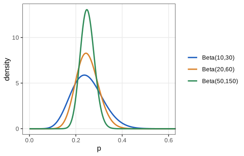
fig_2_19. Reproduces Holmes and Huber (2019), Figure 2.19. PDF · SVG2.9.3 The distribution of \(Y\)
Section 2.9.3 If \(p\) itself is random, \(Y\) has a marginal distribution that mixes binomials over the prior. The book simulates it with the prior \(\BetaD(50,350)\) (mean 0.125, standard deviation 0.0165): draw \(10^5\) values of \(p\), then one \(Y\sim\Bin(300,p)\) for each. (The vectorised call rbinom(length(rp), size = 300, prob = rp) gives the same numbers as the loop with the same seed, Question 2.18, because R draws them in the same order.)
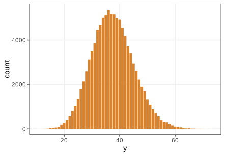
fig_2_20. Reproduces Holmes and Huber (2019), Figure 2.20. PDF · SVGFilling the gap 2.15: the beta-binomial distribution Section 2.9.3, Figure 2.20
The book simulates the marginal distribution of \(Y\). It has a closed form, and its variance shows why mixing over \(p\) inflates the spread.
Derivation
Probability mass function. With \(p\sim\BetaD(\alpha,\beta)\) and \(Y\given p\sim\Bin(n,p)\),
\[ \Prob(Y=y)=\int_0^1\binom nyp^y(1-p)^{n-y}\,\frac{p^{\alpha-1}(1-p)^{\beta-1}}{\mathrm B(\alpha,\beta)}\,\d p=\binom ny\frac{\mathrm B(\alpha+y,\beta+n-y)}{\mathrm B(\alpha,\beta)},\qquad y=0,\dots,n, \]using the Beta integral of Result 2.7. This is the beta-binomial distribution \(\BB(n,\alpha,\beta)\). For \(n=300\), \(\BetaD(50,350)\): \(\Prob(Y=40)=0.0479\) (it agrees with numerical integration, to \(10^{-15}\), and with the simulation, 0.0492).
Mean and variance. Let \(\mu=\alpha/(\alpha+\beta)\) and \(s=\alpha+\beta\). By the tower rule, \(\E Y=\E[np]=n\mu\). By the law of total variance, \(\var Y=\E[\var(Y\given p)]+\var(\E[Y\given p])=n\E[p(1-p)]+n^2\var p\). From Result 2.7, \(\var p=\mu(1-\mu)/(s+1)\) and \(\E[p(1-p)]=\mu-\E p^2=\mu(1-\mu)s/(s+1)\). Hence
\[ \var Y=n\mu(1-\mu)\,\frac{s+n}{s+1}. \]The factor \((s+n)/(s+1)\ge1\) is the overdispersion relative to \(\Bin(n,\mu)\): here \(700/401=1.75\), giving variance \(57.3\) against \(32.8\). It tends to 1 as \(s\to\infty\) (a prior concentrated at one value) and to \(n\) as \(s\to0\). The same mechanism, a Poisson mean varying according to a Gamma distribution, produces the negative binomial used for sequencing counts in Chapter 4 and Chapter 8. ∎
2.9.4 Histogram of all the \(p\)s such that \(Y=40\): the posterior distribution
Section 2.9.4 Keeping only the simulated pairs with \(Y=40\) and looking at their \(p\) values gives a sample from the posterior. In the course run, 4915 of the \(10^5\) draws are kept.
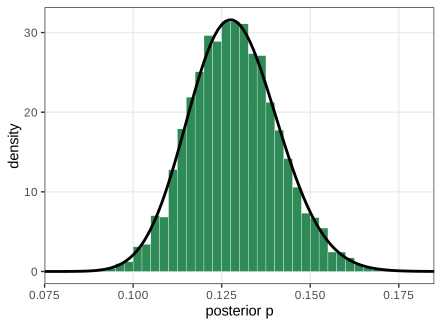
fig_2_21. Reproduces Holmes and Huber (2019), Figure 2.21. PDF · SVGFilling the gap 2.16: why conditioning the simulation gives exact posterior draws Section 2.9.4, Question 2.19
Derivation
Exactness. Each simulated pair \((p_i,Y_i)\) is an independent draw from the joint distribution with density \(\pi(p)\,\Prob(Y=y\given p)\). For any set \(A\subseteq[0,1]\),
\[ \Prob(p_i\in A\given Y_i=40)=\frac{\int_A\pi(p)\Prob(Y=40\given p)\,\d p}{\Prob(Y=40)}=\int_A\pi(p\given Y=40)\,\d p, \]so the kept \(p_i\) are independent draws from the posterior, exactly, with no approximation: \(Y\) is discrete, so "\(Y_i\) equals the observed value" is an event of positive probability. This is rejection sampling (and the simplest case of approximate Bayesian computation, which is needed when the data are continuous and one must accept \(Y_i\) close to the observed value).
Cost. A draw is kept with probability \(\Prob(Y=40)=0.0479\), the marginal of Filling the gap 2.15; from \(10^5\) draws about 4800 survive, so about 95% of the work is discarded. For larger \(n\) or many parameters the acceptance probability becomes tiny, which is why the method is used for illustration rather than in practice.
Monte Carlo accuracy. The posterior standard deviation is \(\sqrt{90\cdot610/(700^2\cdot701)}=0.0126\), so the mean of \(m\approx4900\) kept draws has standard error \(0.0126/\sqrt m=0.00018\). The book's comparison of 0.1285018 (simulation) with 0.1285714 (theory) therefore agrees to the expected 3 to 4 significant digits.
Question 2.19. pPostEmp uses only the ability to simulate the model and needs no algebra, but wastes most draws. pPostMC, drawn directly with rbeta(n, 90, 610), needs the closed-form posterior of Result 2.8 but uses every draw. Both are samples from the same distribution, which the QQ plot of Figure 2.22 confirms. ∎
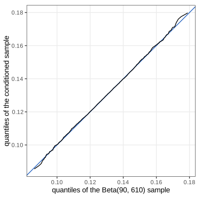
fig_2_22. Reproduces Holmes and Huber (2019), Figure 2.22. PDF · SVG2.9.5 The posterior distribution is also a Beta
Section 2.9.5 The book states, and demonstrates by simulation, that the posterior is \(\BetaD(90,610)\), with parameters obtained by adding the 40 successes to \(\alpha=50\) and the 260 failures to \(\beta=350\). (The book prints the general rule as \(\text{Beta}(\alpha+y,\text{Beta}+(n-y))\); the second argument should read \(\beta+(n-y)\).)
Result 2.8 (Beta-binomial conjugacy) Sections 2.9.2 and 2.9.5
If \(p\sim\BetaD(\alpha,\beta)\) and \(Y\given p\sim\Bin(n,p)\), then \(p\given Y=y\sim\BetaD(\alpha+y,\ \beta+n-y)\). Its mean, mode (MAP estimate) and variance are
\[ \E[p\given y]=\frac{\alpha+y}{\alpha+\beta+n},\qquad \widehat p_{\text{MAP}}=\frac{\alpha+y-1}{\alpha+\beta+n-2},\qquad \var(p\given y)=\frac{(\alpha+y)(\beta+n-y)}{(\alpha+\beta+n)^2(\alpha+\beta+n+1)}. \]Filling the gap 2.17: proof of conjugacy, and the posterior mean as shrinkage Sections 2.9.2 ("we will not prove it here") and 2.9.5
Proof
Conjugacy. By Bayes' theorem, as a function of \(p\),
\[ \pi(p\given y)\ \propto\ p^y(1-p)^{n-y}\cdot p^{\alpha-1}(1-p)^{\beta-1}=p^{(\alpha+y)-1}(1-p)^{(\beta+n-y)-1},\qquad0<p<1. \]The right side is the kernel of the \(\BetaD(\alpha+y,\beta+n-y)\) density (2.6). Two densities that are proportional must be equal (both integrate to 1), so the posterior is that Beta distribution and the normalising constant is \(1/\mathrm B(\alpha+y,\beta+n-y)\); the binomial coefficient and \(m(y)\) never need to be computed. The moments and mode follow from Result 2.7. Normalising prior \(\times\) likelihood numerically on a grid also recovers the \(\BetaD(90,610)\) density.
Shrinkage. Write the posterior mean as a weighted average:
\[ \E[p\given y]=\frac{\alpha+\beta}{\alpha+\beta+n}\cdot\frac{\alpha}{\alpha+\beta}+\frac{n}{\alpha+\beta+n}\cdot\frac yn=w\,\mu_{\text{prior}}+(1-w)\,\widehat p_{\text{MLE}},\qquad w=\frac{\alpha+\beta}{\alpha+\beta+n}. \]The posterior mean shrinks the maximum-likelihood estimate towards the prior mean, and the prior counts as \(\alpha+\beta\) pseudo-observations, of which \(\alpha\) are successes. For the example \(w=400/700=4/7\): the posterior mean \(0.1286\) lies between the prior mean \(0.125\) and \(\widehat p=0.1333\), closer to the prior because the prior is "worth" 400 observations against 300 real ones.
The prior is eventually swamped. For fixed \(\alpha,\beta\) and \(y/n\to p_0\) as \(n\to\infty\), \(w\to0\), the posterior mean tends to \(p_0\) and the posterior variance is about \(p_0(1-p_0)/n\to0\): the posterior concentrates at \(p_0\) whatever the prior. More precisely, the Bernstein-von Mises theorem says that the posterior is then approximately \(\N(\widehat p,\widehat p(1-\widehat p)/n)\), the same normal approximation as the sampling distribution of the MLE (Result 2.2), so Bayesian and frequentist intervals agree to first order. The MAP estimate is \(89/698=0.1275\). ∎
2.9.6 Suppose we had a second series of data
Section 2.9.6 A second sample has 25 carriers among 150 men. Using \(\BetaD(90,610)\) as the new prior, the posterior is \(\BetaD(115,735)\), with mean \(115/850=0.1353\) and mode \(114/848=0.1344\). The answer is the same as if both series had been analysed at once, starting from \(\BetaD(50,350)\) with 65 successes in 450 trials.
Filling the gap 2.18: sequential and batch updating agree, and how much the prior matters Section 2.9.6, Question 2.20
Derivation
In general. If data sets \(D_1,D_2\) are conditionally independent given \(\theta\), then \(\pi(\theta\given D_1,D_2)\propto f(D_2\given\theta)f(D_1\given\theta)\pi(\theta)\propto f(D_2\given\theta)\,\pi(\theta\given D_1)\): the posterior from \(D_1\) is the prior for \(D_2\), and the order of the data does not matter. For the Beta-binomial model the parameters simply accumulate: \(\BetaD(\alpha+y_1+y_2,\ \beta+(n_1-y_1)+(n_2-y_2))\).
A softer prior (Question 2.20). With the uniform prior \(\BetaD(1,1)\), both series together give \(\BetaD(66,386)\): mean 0.146 and 95% interval \([0.115,0.180]\), against mean 0.135 and \([0.113,0.159]\) with \(\BetaD(50,350)\). Here the prior does matter, because it carries 400 pseudo-observations against 450 real ones. The book's general advice (the prior rarely matters unless it is very peaked or the data are few) applies once \(n\gg\alpha+\beta\).
Prediction. Before seeing the second series, the posterior predictive distribution of the number of carriers among \(m=150\) new men is beta-binomial, \(\BB(150,90,610)\) (Filling the gap 2.15 with the posterior in place of the prior): mean \(150\cdot90/700=19.3\), and \(\Prob(Y_2=25)=0.037\). It is wider than \(\Bin(150,0.129)\), because it includes the remaining uncertainty about \(p\). ∎
2.9.7 Confidence statements for the proportion parameter
Section 2.9.7 A credible interval is an interval with a stated posterior probability. The book takes the 2.5% and 97.5% quantiles of \(10^6\) draws from \(\BetaD(115,735)\), \([0.1131,0.1590]\).
Filling the gap 2.19: equal-tailed and highest-density intervals Section 2.9.7
Derivation
Equal-tailed interval. \([Q(0.025),Q(0.975)]\), with \(Q\) the posterior quantile function. For a Beta posterior no simulation is needed: qbeta(c(0.025, 0.975), 115, 735) gives \([0.11314,0.15907]\); the book's Monte Carlo values differ from these by less than \(3\times10^{-4}\).
Highest posterior density (HPD) interval. The shortest interval \([a,b]\) with posterior probability 0.95. Minimise \(b-a\) subject to \(F(b)-F(a)=0.95\). With a Lagrange multiplier \(\lambda\): \(\partial/\partial a\): \(-1+\lambda f(a)=0\), \(\partial/\partial b\): \(1-\lambda f(b)=0\), so \(f(a)=f(b)\). For a unimodal density this means the interval is a level set \(\{p:\pi(p\given y)\ge k\}\): every point inside is more probable than every point outside. For \(\BetaD(115,735)\), \([0.11260,0.15847]\), slightly to the left of the equal-tailed interval because the density is right-skewed; the densities at both ends are equal and the coverage is 0.95.
Interpretation. "\(\Prob(0.113\le p\le0.159\given\text{data})=0.95\)" is a probability statement about \(p\) given the data and the prior. A 95% confidence interval is a statement about a procedure: over repeated samples, 95% of the intervals it produces cover the fixed true \(p\). By the Bernstein-von Mises theorem (Filling the gap 2.17) the two nearly coincide for large \(n\) and a prior that does not dominate. ∎
Shrinkage in practice. The book's Figure 2.23 shows an example from Love et al. (2014): in the DESeq2 method, the log fold change (LFC) of each gene gets a normal prior centred at 0, estimated from all genes, and the reported estimate is the posterior mode. Genes whose likelihood is wide (little information) are shrunk strongly; well-measured genes hardly move. The figure below recomputes this on the pasilla RNA-seq data used in Chapter 8.
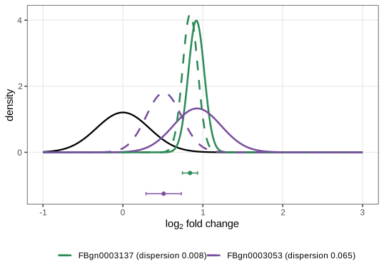
pasilla genes with nearly the same maximum-likelihood LFC (0.92 and 0.93) but different dispersions (0.008 and 0.065), and the normal prior \(\N(0,0.109)\) that DESeq2 estimates from all genes (black). Points with bars: posterior mode \(\pm\) one posterior standard deviation. The low-dispersion gene moves from 0.92 to 0.84, the high-dispersion gene from 0.93 to 0.51; the posterior modes agree with lfcShrink(type = "normal") to 0.003. The likelihood is the negative binomial likelihood with the intercept profiled out (Filling the gap 2.20). Code: fig_2_23. Recomputes on the pasilla data the idea of Holmes and Huber (2019), Figure 2.23 (which shows a published figure of Love et al. 2014). PDF · SVGFilling the gap 2.20: normal-normal shrinkage, and why wide likelihoods shrink more Section 2.9.7, Figure 2.23
Derivation
The normal model. Suppose the estimate \(\widehat b\) of a gene's LFC \(b\) is approximately \(\N(b,s^2)\) with known standard error \(s\), and the prior is \(b\sim\N(0,\tau^2)\). Completing the square in \(b\) in \(-\tfrac12[(b-\widehat b)^2/s^2+b^2/\tau^2]\) gives the posterior
\[ b\given\widehat b\ \sim\ \N\Big(\frac{\tau^2}{\tau^2+s^2}\,\widehat b,\ \frac{\tau^2s^2}{\tau^2+s^2}\Big). \]The posterior mean multiplies \(\widehat b\) by the shrinkage factor \(\tau^2/(\tau^2+s^2)\in(0,1)\): close to 1 when the gene is precisely measured (\(s\ll\tau\)), close to 0 when it is not. The posterior variance is smaller than both \(s^2\) and \(\tau^2\). This is the continuous analogue of Filling the gap 2.17: prior and data are averaged with weights equal to their precisions \(1/\tau^2\) and \(1/s^2\).
Applied to Figure 2.23. With \(\tau^2=0.109\), the observed shrinkage factors \(0.84/0.92=0.917\) and \(0.51/0.93=0.552\) correspond to \(s=0.100\) and \(s=0.298\); the formula then predicts posterior standard deviations \(0.100\sqrt{0.917}=0.095\) and \(0.298\sqrt{0.552}=0.221\), exactly the curvature-based values computed from the full negative binomial posterior (0.095 and 0.221). The higher dispersion of the second gene inflates its standard error threefold, and the prior pulls it most of the way to 0.
What the code computes. For each gene, with size factors \(s_j\) and dispersion \(a\) fixed at DESeq2's estimates, the counts are \(K_j\sim\mathrm{NB}(\mu_j,a)\) with \(\log_2\mu_j=\log_2s_j+\beta_0+bx_j\), \(x_j\) the treatment indicator. For each \(b\) on a grid the intercept \(\beta_0\) is maximised out (profile likelihood), the result is multiplied by the normal prior and normalised. The joint posterior mode of \((\beta_0,b)\) under a flat prior on \(\beta_0\) is the maximiser of this profile, which is why it matches lfcShrink. ∎
2.10 Example: occurrence of a nucleotide pattern in a genome
Section 2.10 The Biostrings package stores sequences as DNAString and DNAStringSet objects, and BSgenome packages provide whole genomes (Question 2.21: GENETIC_CODE is the codon table, IUPAC_CODE_MAP the ambiguity codes). The example counts the Shine-Dalgarno motif AGGAGGT, which helps ribosomes bind bacterial messenger RNA, along the 4,686,137 bases of E. coli K-12 DH10B (accession NC_010473), on the given strand and without mismatches. In the 93 complete windows of 50,000 bases the counts are:
| Matches per window \(k\) | 0 | 1 | 2 | 3 | 4 |
|---|---|---|---|---|---|
| Windows observed | 48 | 32 | 8 | 3 | 2 |
| Expected, \(\Pois(0.699)\) | 46.2 | 32.3 | 11.3 | 2.6 | 0.5 |
A Poisson model (Question 2.22) fits: \(G^2=4.13\) on 3 degrees of freedom, \(p=0.25\) (Filling the gap 2.3). The book also shows distplot, a "Poissonness" plot.
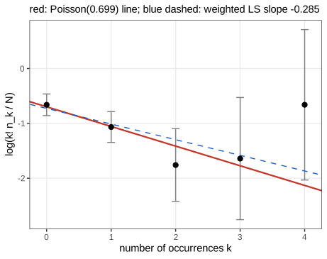
fig_2_24 (my implementation of the plot that vcd::distplot draws). Reproduces Holmes and Huber (2019), Figure 2.24. PDF · SVGFilling the gap 2.21: the Poissonness plot Section 2.10, Figure 2.24
Derivation
Linearisation. If the \(N\) values are \(\Pois(\lambda)\), the expected frequency of \(k\) is \(Ne^{-\lambda}\lambda^k/k!\). Taking logarithms of \(n_k\approx Ne^{-\lambda}\lambda^k/k!\) and rearranging,
\[ \phi(n_k)=\log\frac{k!\,n_k}{N}\approx-\lambda+k\log\lambda, \]a straight line in \(k\) with slope \(\log\lambda\) and intercept \(-\lambda\) (Hoaglin, 1980). Curvature indicates another distribution: for example, the negative binomial makes the metameter bend upwards. The slope gives a graphical estimate of \(\lambda\); here the weighted least-squares slope \(-0.285\) corresponds to \(\lambda\approx0.75\), close to \(\widehat\lambda=0.699\) (slope \(-0.358\)).
Error bars by the delta method. \(n_k\sim\Bin(N,p_k)\) has variance \(Np_k(1-p_k)\), and \(\var(\log n_k)\approx\var(n_k)/(Np_k)^2=(1-p_k)/(Np_k)\). Replacing \(Np_k\) by \(n_k\) gives the standard error \(\sqrt{(1-n_k/N)/n_k}\) used for the bars. A simulation confirms the formula to 3% for \(N=500\), \(p_k=0.22\). Hoaglin and Tukey's version of the plot used by distplot adds a small-count correction to \(n_k\); the idea is the same. ∎
The 65 matches split the genome into 66 gaps (Biostrings' gaps counts the stretch before the first and after the last match). If motifs occurred at random, the gaps would be approximately exponential.
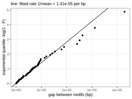
ppoints, and the line with the fitted rate \(1/\bar g=1.41\times10^{-5}\) per base (mean gap 71,000 bases). The largest gaps lie to the right of the line: the tail is heavier than exponential. Code: fig_2_25. Reproduces Holmes and Huber (2019), Figure 2.25 (drawn by Renext::expplot in the book). PDF · SVGFilling the gap 2.22: why gaps are exponential, and why the tail is heavier Section 2.10, footnote on the exponential, Question 2.23
Derivation
From Bernoulli occurrences to the exponential. Suppose each position independently starts a motif with a small probability \(p\) (ignoring overlaps). The distance \(G\) from one occurrence to the next is geometric: \(\Prob(G>t)=(1-p)^t=e^{t\log(1-p)}\). Since \(\log(1-p)=-p-p^2/2-\dots\), \((1-p)^t\approx e^{-pt}\) with relative error about \(tp^2/2\), negligible for \(p\approx10^{-5}\) and \(t\) up to \(10^6\) (it is below \(2\times10^{-4}\) for \(p=10^{-4}\), \(t\le3\times10^4\)). So \(G\) is approximately \(\Exp(p)\), with mean \(1/p\).
MLE of the rate. For independent \(g_1,\dots,g_m\sim\Exp(r)\), \(\ell(r)=m\log r-r\sum_ig_i\), with \(\ell'(r)=m/r-\sum g_i=0\) at \(\widehat r=1/\bar g\) and \(\ell''=-m/r^2<0\): the line in Figure 2.25 uses the MLE.
Why the right tail deviates (Question 2.23). A constant rate is unrealistic: gene density, strand and base composition vary along the genome. If the rate itself varies, the gaps follow a mixture of exponentials, \(\Prob(G>t)=\sum_jw_je^{-r_jt}\). Its hazard \(h(t)=\sum_jw_jr_je^{-r_jt}/\sum_jw_je^{-r_jt}\) is a weighted average of the \(r_j\) whose weights move towards the small rates as \(t\) grows, so \(h\) decreases: long gaps become relatively more likely than under a single exponential with the same mean. In the exponential plot \(-\log\Prob(G>t)=\int_0^th\) is concave, which puts the largest observed gaps to the right of the fitted line, as seen. Two further reasons: the first and last "gaps" are not between two motifs (the genome is circular, but the sequence is stored linearly), and with only 66 gaps the extreme order statistics are very variable. ∎
2.10.1 Modeling in the case of dependencies
Section 2.10.1 CpG islands are stretches of DNA rich in the dinucleotide CG (the C followed by G on the same strand); elsewhere CG is rare because methylated cytosines in CG mutate easily. The book takes the model-based CpG islands of Irizarry et al. (2009) on chromosome 8 of the human genome (hg19), 2855 islands, and the 2854 stretches between them.
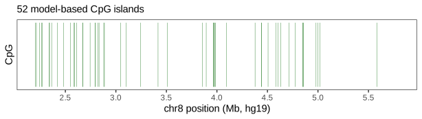
fig_2_26. Reproduces Holmes and Huber (2019), Figure 2.26. PDF · SVGCounting the transitions inside islands and outside them, and normalising each row (Result 2.6), gives two transition matrices (rows: from; columns: to):
| Islands | A | C | G | T | Elsewhere | A | C | G | T | |
|---|---|---|---|---|---|---|---|---|---|---|
| A | 0.205 | 0.265 | 0.390 | 0.140 | A | 0.335 | 0.168 | 0.231 | 0.266 | |
| C | 0.201 | 0.344 | 0.237 | 0.217 | C | 0.364 | 0.246 | 0.042 | 0.348 | |
| G | 0.187 | 0.315 | 0.345 | 0.154 | G | 0.298 | 0.203 | 0.247 | 0.253 | |
| T | 0.098 | 0.335 | 0.360 | 0.207 | T | 0.227 | 0.197 | 0.241 | 0.335 | |
| Letters | 0.178 | 0.320 | 0.321 | 0.181 | Letters | 0.301 | 0.199 | 0.199 | 0.300 |
The rows differ within each matrix (Question 2.24: in islands \(\Prob(\tA\given\tC)=0.201\) but \(\Prob(\tA\given\tT)=0.098\)), so the letters are not independent, and the matrices differ from each other, most of all in \(\Prob(\tG\given\tC)\): 0.237 in islands, 0.042 elsewhere. Islands are also GC-rich (Question 2.25). A chi-square comparison of letter frequencies (Question 2.26) uses only the composition; a likelihood ratio between the two chains also uses the transitions and is more sensitive for short sequences.
For a sequence \(x=x_1\cdots x_L\), the log-likelihood-ratio score of island versus non-island is
\[ \log\frac{\Prob(x\given\text{island})}{\Prob(x\given\text{non-island})}=\log\frac{\pi^{\mathrm i}_{x_1}}{\pi^{\mathrm n}_{x_1}}+\sum_{t=2}^L\log\frac{P^{\mathrm i}_{x_{t-1}x_t}}{P^{\mathrm n}_{x_{t-1}x_t}}=\alpha_{x_1}+\sum_{t=2}^L\beta_{x_{t-1}x_t}, \tag{2.7} \]with \(\alpha\) and \(\beta\) the log-ratios of the letter frequencies and of the transition probabilities, computed once and then added up. For the book's example \(x=\) ACGTTATACTACG (13 letters, 12 transitions) the terms are \(\alpha_\tA=-0.524\) and \(\beta\) values \(0.457\) (AC), \(1.737\) (CG), \(-0.497\) (GT), \(-0.482\) (TT), \(-0.838\) (TA), \(-0.639\) (AT), \(-0.838\) (TA), \(0.457\) (AC), \(-0.470\) (CT), \(-0.838\) (TA), \(0.457\) (AC), \(1.737\) (CG), with total \(-0.2825\), the book's value. (The book's displayed product for this example lists only nine transitions; the three in the middle, CT, TA, AC, are missing, though its code sums all twelve.)
Filling the gap 2.23: why the log-likelihood ratio is the right score Section 2.10.1, (2.7), Figure 2.27
Derivation
Derivation of (2.7). Apply Result 2.6 to each model: \(\Prob(x\given\text{island})=\pi^{\mathrm i}_{x_1}\prod_{t\ge2}P^{\mathrm i}_{x_{t-1}x_t}\), likewise for non-islands, and take the log of the ratio. Numerically, the sum of \(\alpha\) and \(\beta\) terms equals the log of the ratio of the two products, to \(10^{-15}\). (The initial distribution is estimated by the overall letter frequencies, which are within 0.002 of the stationary distributions of the two chains.)
Optimality. By the Neyman-Pearson lemma, among all rules that call a non-island sequence an island with probability at most \(\alpha\), the rule "island if the score exceeds a threshold \(c\)" has the largest probability of detecting a true island. Proof sketch: for any rule with acceptance region \(R\) and the likelihood-ratio region \(R^*=\{x:\Lambda(x)>c\}\), \(\sum_x(\mathbb 1_{R^*}-\mathbb 1_R)(P_{\mathrm i}(x)-e^cP_{\mathrm n}(x))\ge0\) term by term, which rearranges to \(P_{\mathrm i}(R^*)-P_{\mathrm i}(R)\ge e^c[P_{\mathrm n}(R^*)-P_{\mathrm n}(R)]\ge0\) when \(P_{\mathrm n}(R)\le P_{\mathrm n}(R^*)\). With prior probabilities of the two classes, the posterior log-odds is the score plus the log prior odds, so the Bayes classifier (fewest misclassifications) also thresholds the score, at \(c=\log(\pi_{\text{non}}/\pi_{\text{island}})\).
What a per-base score measures. Divide the score by \(L\). For a long sequence generated by the island chain, the ergodic theorem for Markov chains gives
\[ \frac1L\sum_t\beta_{x_{t-1}x_t}\ \to\ \sum_{x,y}\pi^{\mathrm i}_xP^{\mathrm i}_{xy}\log\frac{P^{\mathrm i}_{xy}}{P^{\mathrm n}_{xy}}=0.176, \]the Kullback-Leibler divergence rate between the chains, which is positive by Gibbs' inequality; for background sequences the limit is minus the reverse divergence rate, \(-0.150\). Sequences simulated from the island chain have mean per-base score 0.177. A central limit theorem for Markov chains makes the spread of the per-base score shrink like \(1/\sqrt L\), so the two classes separate as windows get longer: at \(L=100\) and threshold 0, 10.5% of island windows and 10.3% of background windows are misclassified.
Why the island histogram looks like a mixture. The islands are model-based intervals: some contain stretches that look like ordinary sequence, and windows drawn from such stretches score like background. The histogram of island scores is then a mixture of a high-scoring and a lower component, the book's first encounter with mixture models (Chapter 4). ∎
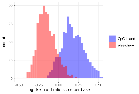
fig_2_27. Reproduces Holmes and Huber (2019), Figure 2.27. PDF · SVGThese windows are training data: sequences of known class used to build and calibrate a classifier, a theme developed in Chapter 12.
Summary
- Statistical models. A model is a family of distributions indexed by a few parameters. The binomial, multinomial and Poisson families cover categorical and count data; a Markov chain adds dependence along a sequence; Hardy-Weinberg and the position weight matrix are multinomials with structure.
- Estimation. Maximum likelihood gives the sample mean (Poisson), the observed proportion (binomial), the observed frequencies (multinomial), allele counting (Hardy-Weinberg) and row-normalised transition counts (Markov chain). The curvature of the log-likelihood, the Fisher information, gives standard errors; Wald and likelihood-ratio intervals follow.
- Goodness of fit. Rootograms (square roots stabilise the variance), Poissonness and exponential plots, QQ plots, and the Pearson and likelihood-ratio statistics, which are asymptotically chi-square with (cells \(-\) 1 \(-\) estimated parameters) degrees of freedom. When the theory is doubtful, simulation (parametric bootstrap) or permutation gives a valid reference distribution.
- Bayesian estimation. With a Beta prior and binomial data the posterior is Beta; its mean is a precision-weighted compromise between prior mean and data, data can be added one series at a time, and the prior matters only when it carries as much information as the data. Credible intervals come directly from posterior quantiles. Normal priors shrink noisy estimates (DESeq2's fold changes) most.
- Sequences. Motif counts in windows can be Poisson and gaps between motifs roughly exponential, with a heavier tail when the rate varies. Two Markov chains, one for CpG islands and one for the rest, give a log-likelihood-ratio score that is the optimal classifier and whose per-base mean is a Kullback-Leibler divergence rate; its histogram on real windows is a first example of a mixture.
Exercises
The six exercises of Chapter 2 (Holmes and Huber, 2019, Section 2.13), restated in my own words, with worked solutions (hidden).
Exercise 2.1. Model mutations along a gene of length 1000 as independent 0/1 events with probability \(10^{-4}\) per position, and count the mutations in a sequence. Repeat many times, find the distribution of the count by a goodness-of-fit test and plot the fit.
Solution
The count is exactly \(\Bin(1000,10^{-4})\), and by the Poisson limit it is very close to \(\Pois(0.1)\): Le Cam's inequality bounds the total variation distance by \(np^2=10^{-5}\) (the exact distance is below the bound). Simulating 1000 sequences (seed 21) gives 913 zeros, 80 ones and 7 twos; \(\widehat\lambda=0.094\) and Pearson's \(X^2=2.58\). With almost all values 0 or 1, cells must be pooled (expected count at least about 5), which leaves very few degrees of freedom; a rootogram from
goodfit(x, "poisson")(as in Figure 2.3) shows bars ending close to the axis. The exercise is a reminder that a goodness-of-fit test can only distinguish distributions that differ where the data are, and that binomial and Poisson are indistinguishable here.Exercise 2.2. Write a function returning the maximum of \(n\) uniform random numbers on \([0,7]\); run it for \(n=25\), repeat 100 times and plot the maxima. What is the maximum-likelihood estimate \(\widehat\theta\) of the upper end \(\theta\) of a uniform distribution on \([0,\theta]\) from a sample of size 25? Justify it and relate it to the true \(\theta\).
Solution
MLE. The likelihood of \(\theta\) is \(L(\theta)=\prod_i\theta^{-1}\mathbb 1\{0\le x_i\le\theta\}=\theta^{-n}\mathbb 1\{\theta\ge x_{(n)}\}\), where \(x_{(n)}=\max_ix_i\). It is zero for \(\theta<x_{(n)}\) and strictly decreasing for \(\theta\ge x_{(n)}\), so \(\widehat\theta=x_{(n)}\). Setting a derivative to zero would fail: the maximum is at a boundary where \(L\) jumps.
Sampling distribution. \(\Prob(X_{(n)}\le t)=(t/\theta)^n\) for \(0\le t\le\theta\), with density \(nt^{n-1}/\theta^n\). Hence \(\E X_{(n)}=n\theta/(n+1)\) and \(\var X_{(n)}=n\theta^2/\{(n+1)^2(n+2)\}\). For \(\theta=7\), \(n=25\): mean \(6.731\), standard deviation \(0.259\) (20,000 simulated maxima give mean 6.731). The MLE is biased downwards by \(\theta/(n+1)\) (it can never exceed \(\theta\)); \((n+1)X_{(n)}/n\) is unbiased. The histogram of maxima piles up just below 7 with a long left tail.
Non-regular. The support depends on \(\theta\), so the Fisher-information theory of Filling the gap 2.2 does not apply: the error \(\theta-X_{(n)}\) is of order \(1/n\), not \(1/\sqrt n\), and \(n(\theta-X_{(n)})/\theta\) converges to an exponential distribution, not a normal one.
Exercise 2.3. Each amino acid is coded by one to six codons, and the different codons of an amino acid are not used equally often. Using the codon counts of M. tuberculosis H37Rv (
M_tuberculosis.txt): tabulate amino acids against codons, explain how the columnPerThouswas made, and write a function that finds the amino acid with the strongest codon bias.Solution
Table and
PerThous.table(mtb$AmAcid)shows the multiplicities (Leu, Ser, Arg 6; Ala, Gly, Pro, Thr, Val 4; Ile and the stop "End" 3; Met and Trp 1; the rest 2), 64 codons in all.PerThousis the count per thousand codons of the genome, \(1000\times\)Number\(/1{,}344{,}223\) (this holds to rounding). The proline proportions are 0.543, 0.105, 0.059, 0.293.Measuring bias. For an amino acid with \(k\) codons and observed proportions \(\widehat{\bm p}\), the departure from uniform use can be measured by the Kullback-Leibler divergence \(\sum_j\widehat p_j\log(k\widehat p_j)\) (between 0 and \(\log k\)), possibly divided by \(\log k\). A chi-square statistic against equal proportions is not a good measure of strength: every amino acid has thousands of codons, all tests reject with p-values below \(10^{-100}\), and \(X^2\) grows with the count rather than with the bias (Leu has the largest \(X^2\) only because it is the most frequent).
Result. Isoleucine has the strongest bias by either version of the divergence (0.478 nats, 0.435 of its maximum \(\log3\)): 80% of its codons are ATC, against 19% ATT and 6% ATA. Then come Leu (0.456; CTG 52%), Arg (0.372) and Thr (0.356). This reflects the high GC content of the M. tuberculosis genome, which favours codons ending in C or G. A function: split the table by amino acid, drop single-codon amino acids, compute the divergence for each and return the maximum (five lines of R do exactly this).
Exercise 2.4. Read the S. aureus sequences from
staphsequence.ffn.txt, look at the first three, compute the GC content in sliding windows of width 100 along a sequence, plot it, and show the overall trend.Solution
The set contains 2650 sequences (widths 1362, 1134, 246 for the first three).
letterFrequencyInSlidingView(s, 100, c("G", "C"))returns, for every window start, the counts of G and C; their sum divided by 100 is the GC fraction. Figure 2.28 shows it for sequence 364; a lowess smooth with span 0.2 (Figure 2.29) shows the trend. The genome-wide GC content per gene can be computed withalphabetFrequency, as the book does. Deciding where the GC content is abnormally high calls for a model with hidden states (a hidden Markov model), the same idea that defined the CpG islands of Section 2.10.1.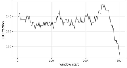
Figure 2.28. GC fraction in sliding windows of width 100 along sequence 364. Code: fig_2_28. Reproduces Holmes and Huber (2019), Figure 2.28. PDF · SVG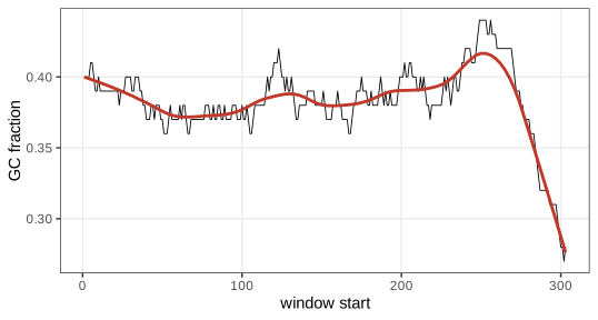
Figure 2.29. As Figure 2.28 with a lowess smooth (span 0.2, red). Code: fig_2_29. Reproduces Holmes and Huber (2019), Figure 2.29. PDF · SVGExercise 2.5. Redraw Figure 2.19 adding the uniform distribution \(\BetaD(1,1)\) and \(\BetaD(\tfrac12,\tfrac12)\). What do you notice?
Solution
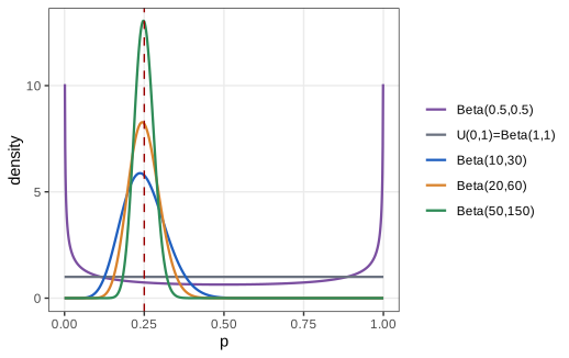
Figure 2.30. \(\BetaD(\tfrac12,\tfrac12)\), \(\BetaD(1,1)\) and the three priors of Figure 2.19; the dashed line marks 0.25. Code: fig_2_30. Reproduces Holmes and Huber (2019), Figure 2.30. PDF · SVGWith \(\alpha,\beta>1\) the density is unimodal and vanishes at both ends. \(\BetaD(1,1)\) is flat: every \(p\) is equally likely a priori, and the posterior after \(y\) of \(n\) is \(\BetaD(y+1,n-y+1)\), whose mode is the MLE \(y/n\). \(\BetaD(\tfrac12,\tfrac12)\) is U-shaped, with density tending to infinity at 0 and 1 (the book calls it bimodal; strictly, its density is unbounded at both ends and has its minimum at \(1/2\)). Its mean is \(1/2\), not \(1/4\). It is the Jeffreys prior of the binomial model: proportional to \(\sqrt{I(p)}=\{p(1-p)\}^{-1/2}\) with \(I\) the Fisher information of Filling the gap 2.4, which makes it invariant under reparametrisation. Both \(\BetaD(1,1)\) and \(\BetaD(\tfrac12,\tfrac12)\) carry the weight of only 2 or 1 pseudo-observations (Filling the gap 2.17), so they are "weak" priors.
Exercise 2.6. Choose your own Beta prior for the haplotype frequency (the book suggests sketching it with an online tool), redo the analysis of Section 2.9.1 with \(y=40\) of \(n=300\), and compare your posterior with the one obtained there using a QQ plot.
Solution
Translate a belief into \((\alpha,\beta)\) through the mean \(\mu\) and the prior sample size \(s=\alpha+\beta\) (Filling the gap 2.17): \(\alpha=\mu s\), \(\beta=(1-\mu)s\). Example: "about 1 in 6, but I would not be surprised by anything between 5% and 35%" suggests \(\mu=1/6\), \(s=12\), i.e. \(\BetaD(2,10)\) (95% prior interval \([0.023,0.413]\)). The posterior is \(\BetaD(42,270)\), mean \(42/312=0.135\), 95% interval \([0.099,0.175]\), against \(\BetaD(90,610)\) (mean 0.129, \([0.105,0.154]\)). A QQ plot of the two posteriors (quantiles from
qbetaatppoints(1000), no simulation needed) is close to a straight line with slope 1.53 (the ratio of the posterior standard deviations, 0.0193 and 0.0126) and a small shift: the two posteriors have nearly the same shape but different spread, because the weak prior lets the 300 observations dominate while \(\BetaD(50,350)\) adds 400 pseudo-observations. The Bayesian updating demo lets you set any prior and see the posterior, its interval and the shrinkage weight.
Demonstrations for this chapter
Each demonstration runs in the browser on data exported by the R code (data/ch02-*.json), uses seeded random numbers, and links back to these notes. The ▶ Demo boxes above open them already set to the case under discussion. Their computations agree with R.
| Demonstration | What you can see | Sections and results |
|---|---|---|
| Likelihood for count data: Poisson, binomial, Hardy-Weinberg | The log-likelihood and its quadratic approximation, MLE, standard error, Wald and likelihood-ratio intervals, rootogram and \(G^2\), and the de Finetti diagram with the acceptance band. Presets: 1 epitope counts (Fig. 2.4); 2 without the outlier (Fig. 2.3); 3 Shine-Dalgarno windows (Fig. 2.24); 4 binomial 40 of 300 (Fig. 2.6); 5 Hardy-Weinberg, Tahiti (Figs. 2.11–2.12). | 2.3 (Gaps 2.1, 2.3), 2.3.1 (Result 2.1), 2.4.2 (Result 2.2), 2.7.2 (Result 2.5, Gap 2.12), 2.10 |
| Pearson's chi-square statistic: simulation against theory | Simulated tables for the first \(G\) S. aureus genes with \(\bm p\) known or re-estimated, histogram and QQ plot against \(\chi^2_{G(K-1)}\) and \(\chi^2_{(G-1)(K-1)}\), small-count failures, and Chargaff's exact permutation distribution. Presets: 1 ten genes, \(\bm p_0\) known (Figs. 2.7–2.8); 2 \(\bm p\) re-estimated: 27 degrees of freedom; 3 small expected counts; 4 Chargaff's rule (Fig. 2.10). | 2.5.2, 2.6 (Result 2.4, Gaps 2.6–2.8), 2.7 (Gap 2.9) |
| Bayesian updating of a proportion | Prior, scaled likelihood and posterior, the shrinkage weight, equal-tailed and HPD intervals, the beta-binomial marginal, and the conditioning simulation. Presets: 1 \(\BetaD(50,350)\) and 40 of 300 (Figs. 2.20–2.21); 2 a second series (Sections 2.9.6–2.9.7); 3 uniform prior (Question 2.20); 4 a weak prior of your own (Exercise 2.6); 5 few data, strong prior. | 2.9 (Results 2.7, 2.8, Gaps 2.15–2.19) |
| Markov chain scores for CpG islands | The two chr8 transition matrices and their log-ratios, the score of any typed sequence term by term, histograms of per-base scores for real island and background windows of adjustable length, threshold and error rates, and sequences simulated from the chains. Presets: 1 the book's example sequence; 2 100-base windows (Fig. 2.27); 3 short windows; 4 simulated chains against real windows; 5 long windows. | 2.8 (Result 2.6, Gap 2.14), 2.10.1 (Gap 2.23) |
The R code that produces every figure of this page is code/ch02_statistical_modeling.R (see the code index).
References
- Holmes, S. and Huber, W. (2019). Modern Statistics for Modern Biology. Cambridge University Press, Cambridge. Chapter 2, "Statistical Modeling".
- Chernoff, H. and Lehmann, E. L. (1954). The use of maximum likelihood estimates in \(\chi^2\) tests for goodness of fit. The Annals of Mathematical Statistics, 25(3), 579–586.
- Durbin, R., Eddy, S. R., Krogh, A. and Mitchison, G. (1998). Biological Sequence Analysis: Probabilistic Models of Proteins and Nucleic Acids. Cambridge University Press, Cambridge.
- Elson, D. and Chargaff, E. (1952). On the desoxyribonucleic acid content of sea urchin gametes. Experientia, 8(4), 143–145.
- Hardy, G. H. (1908). Mendelian proportions in a mixed population. Science, 28(706), 49–50. doi:10.1126/science.28.706.49.
- Hoaglin, D. C. (1980). A Poissonness plot. The American Statistician, 34(3), 146–149.
- Irizarry, R. A., Wu, H. and Feinberg, A. P. (2009). A species-generalized probabilistic model-based definition of CpG islands. Mammalian Genome, 20(9–10), 674–680.
- Le Cam, L. (1960). An approximation theorem for the Poisson binomial distribution. Pacific Journal of Mathematics, 10(4), 1181–1197.
- Love, M. I., Huber, W. and Anders, S. (2014). Moderated estimation of fold change and dispersion for RNA-seq data with DESeq2. Genome Biology, 15, 550. doi:10.1186/s13059-014-0550-8.
- Mourant, A. E., Kopeć, A. C. and Domaniewska-Sobczak, K. (1976). The Distribution of the Human Blood Groups and Other Polymorphisms, 2nd edition. Oxford University Press, London.
- Neyman, J. and Pearson, E. S. (1933). On the problem of the most efficient tests of statistical hypotheses. Philosophical Transactions of the Royal Society of London, Series A, 231, 289–337. doi:10.1098/rsta.1933.0009.
- Pearson, K. (1900). On the criterion that a given system of deviations from the probable in the case of a correlated system of variables is such that it can be reasonably supposed to have arisen from random sampling. Philosophical Magazine, Series 5, 50(302), 157–175. doi:10.1080/14786440009463897.
- Rice, J. A. (2006). Mathematical Statistics and Data Analysis, 3rd edition. Duxbury, Belmont, CA. Chapter 8.
- Schneider, T. D. and Stephens, R. M. (1990). Sequence logos: a new way to display consensus sequences. Nucleic Acids Research, 18(20), 6097–6100. doi:10.1093/nar/18.20.6097.
- Tukey, J. W. (1977). Exploratory Data Analysis. Addison-Wesley, Reading, MA. (Hanging rootograms; the book cites Cleveland, 1988.)
- van der Vaart, A. W. (1998). Asymptotic Statistics. Cambridge University Press, Cambridge. (Wilks' theorem, chi-square tests with estimated parameters, the Bernstein-von Mises theorem.)
- Yates, F. (1934). Contingency tables involving small numbers and the \(\chi^2\) test. Supplement to the Journal of the Royal Statistical Society, 1(2), 217–235.
The numerical statements in the text (maximisers, information, interval endpoints, the exact Chargaff p-value, the degrees-of-freedom simulation, the Hardy-Weinberg closed form, the Beta-binomial identities, the DESeq2 comparison and the CpG divergence rates) are computed by the course code.