Nonparametric Regression
Given pairs \((x_i,Y_i)\) with \(Y_i=r(x_i)+\epsilon_i\), we want the regression function \(r\) without assuming a parametric form. Every estimator of this chapter (regressograms, kernel and local polynomial smoothers, smoothing and regression splines) is a linear smoother: the fitted values are \(\mathbf{L}\bY\) for a smoothing matrix \(\mathbf{L}\) that depends on the \(x\)'s and on one smoothing parameter. That single fact gives the effective degrees of freedom \(\tr\mathbf{L}\), a one-fit formula for leave-one-out cross-validation, an unbiased-in-the-limit variance estimate, and simultaneous confidence bands through the tube formula. The chapter then pays the price of nonparametric inference honestly: the risk decreases like \(n^{-4/5}\) rather than \(n^{-1}\), the bands cover a smoothed version of \(r\) rather than \(r\), and in \(d\) dimensions the sample size has to grow exponentially. It ends with local likelihood for non-Gaussian responses and with additive models, projection pursuit, trees and MARS for several covariates.
Ch. 1 Introduction Ch. 2 The cdf and functionals Ch. 3 Bootstrap and jackknife Ch. 4 Smoothing Ch. 5 Regression Ch. 6 Density estimation Ch. 7 Normal means and minimax Ch. 8 Orthogonal functions Ch. 9 Wavelets Ch. 10 Other topics
How to read these notes
They follow the book. Sections carry the book's numbers (5.1 to 5.16), results keep the book's numbers (Theorem 5.34, Definition 5.39, ...), and every displayed equation of the book keeps its number, e.g. \((5.35)\). Equations without a number are steps the book skips.
Filling the gaps. The chapter states many results without proof ("it can be shown", "a proof can be found in", results quoted from the literature). For each one an orange Filling the gap box gives a complete argument, with its assumptions stated. Proofs and derivations start hidden: open one with its bar, or use the button below.
Figures and demonstrations. Every figure of the chapter that is computed from data or a simulation is reproduced from scratch by the Python code (Figure 5.18, a schematic tree with no data, is not). Supplementary figures (numbered 5.S1, 5.S2, ...) illustrate the gaps and the exercises. The ▶ Demo boxes open an interactive demonstration already set to the case being discussed.
Main reference
L. Wasserman, All of Nonparametric Statistics, Springer (2006), Chapter 5, pages 61–123 (book website, with the data: www.stat.cmu.edu/~larry/all-of-nonpar). Section, equation, figure and exercise numbers below refer to this book. Further reading is listed in the references.
The explanations, derivations, figures and code are my own; equations are cited by their numbers in the book.
Companion courses
This chapter is the advanced sequel of the regression part of Probability and Statistical Inference (the same author's All of Statistics), and it overlaps three other courses on this site:
- Section 5.1 (linear and logistic regression): Probability and Statistical Inference, Section 13.5 (multiple regression) and Section 13.7 (logistic regression).
- Sections 5.2–5.4, 5.6, 5.7 (kernel regression, the leave-one-out shortcut, the difference variance estimator, bands): Probability and Statistical Inference, Section 20.4 (Theorems 20.21 and 20.22, Filling the gaps 20.14 to 20.18) and its kernel regression band demo.
- Sections 5.3–5.5, 5.10 (local regression, splines, cross-validation, local likelihood): Statistical Learning: Theory and Methods, Sections 6.1–6.5, 5.2 and 5.4, and 7.10; Applied Statistical Learning in R and Python, Sections 7.4–7.7.
- Section 5.12 (additive models, projection pursuit, trees, MARS): Statistical Learning, Sections 9.1, 9.2, 9.4 and 11.2; Probability and Statistical Inference, Filling the gap 20.19 (backfitting).
Where a proof there is complete, these notes state the result, sketch the argument and link to it. What this chapter adds, and where the effort goes here: the general theory of linear smoothers, the design and boundary bias of local polynomials, the B-spline machinery, simultaneous bands by the tube formula (with the heteroscedastic version and the price of choosing \(h\)), average coverage, the minimax optimality of local linear regression, and derivative estimation.
The chapter at a glance
- 5.1 Least squares is a projection, \(p=\tr\mathbf{L}\), and Scheffé's band covers a whole regression line (Theorem 5.14); logistic regression is fitted by Newton's method in disguise (Filling the gap 5.2).
- 5.2–5.3 A linear smoother has fitted values \(\mathbf{L}\bY\) and \(\nu=\tr\mathbf{L}\) degrees of freedom; the training error is biased down by exactly \(2\sigma^2\nu/n\) (Filling the gap 5.4); leave-one-out cross-validation needs only one fit (Theorem 5.34).
- 5.4 Kernel regression has risk of order \(n^{-4/5}\) with a design bias \(2r'f'/f\) (Theorem 5.44); local linear regression removes the design bias and the boundary bias at no cost in variance (Theorem 5.65).
- 5.5 The penalised least squares problem is solved by a natural cubic spline with knots at the data (Theorem 5.73), computed in the B-spline basis as a ridge-type linear smoother (Theorem 5.81), which behaves like a kernel smoother with a variable bandwidth (Filling the gap 5.11).
- 5.6 \(\|\bY-\mathbf{L}\bY\|^2/(n-2\nu+\tilde\nu)\) estimates \(\sigma^2\) consistently (Theorem 5.85), as do the difference estimators; the log-residual recipe for \(\sigma^2(x)\) needs a correction of \(1.27\) (Filling the gap 5.14).
- 5.7–5.9 Bands \(\hr\pm c\,\hs\|\bl(x)\|\) cover \(\br=\E\hr\), not \(r\); the tube formula gives \(c\) from \(\kappa_0=\int\|T'\|\) (Filling the gap 5.16, Appendix); a confidence ball gives bands with average coverage (Result 5.108).
- 5.10–5.13 Local likelihood for binary data, SiZer, the curse of dimensionality \(n^{-4/(4+d)}\), additive models, projection pursuit, trees, MARS, plug-in bandwidths, a linearity test, minimax optimality and derivative estimation.
Notation. Data \((x_1,Y_1),\dots,(x_n,Y_n)\), \(\bY=(Y_1,\dots,Y_n)^\T\), \(\mathbf{r}=(r(x_1),\dots,r(x_n))^\T\). An estimator \(\hr\), its mean \(\br(x)=\E\hr(x)\), the weight vector \(\bl(x)=(\ell_1(x),\dots,\ell_n(x))^\T\) and the smoothing matrix \(\mathbf{L}\) with \(L_{ij}=\ell_j(x_i)\). A kernel \(K\) is a symmetric density with \(\mu_2(K)=\int u^2K(u)\,\d u\in(0,\infty)\) and \(R(K)=\int K^2\); unless said otherwise the tricube kernel \(K(u)=\tfrac{70}{81}(1-|u|^3)^3\) on \([-1,1]\), the book's default, is used. \(\Phi,\phi\) are the standard Normal cdf and density.
Prerequisites. Chapter 4 of the book (risk, the bias–variance decomposition, kernels) and least squares. The companion course's Chapter 20 is the gentle version of Sections 5.2–5.7.
p. 61 The model is
\[ Y_i=r(x_i)+\epsilon_i,\qquad \E(\epsilon_i)=0,\qquad i=1,\dots,n, \tag{5.1} \]with \(\V(\epsilon_i)=\sigma^2\) for now. The \(x_i\) are treated as fixed; if they are random, \(r\) is the conditional mean
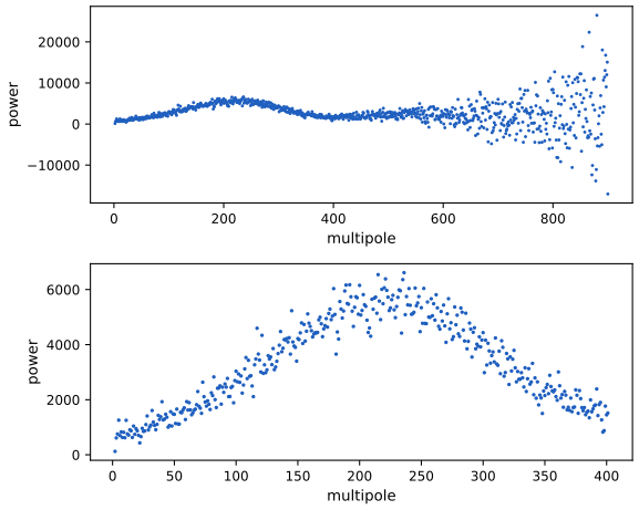
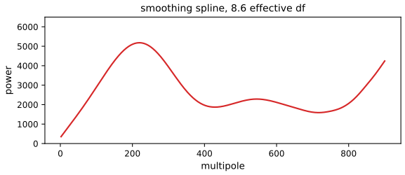
\[ r(x)=\E(Y\given X=x), \tag{5.2} \]and all statements below hold conditionally on \(X_1,\dots,X_n\). The running example is the cosmic microwave background (CMB) power spectrum (Example 5.3): \(x\) is the multipole moment, a frequency of the temperature fluctuations, and \(Y\) the measured power at that frequency.
5.1 Review of Linear and Logistic Regression
pp. 63–66 With covariates \(x_i=(x_{i1},\dots,x_{ip})^\T\) and \(x_{i1}=1\) (the intercept),
\[ Y_i=r(x_i)+\epsilon_i\equiv\sum_{j=1}^p\beta_jx_{ij}+\epsilon_i,\qquad \E(\epsilon_i)=0,\ \V(\epsilon_i)=\sigma^2, \tag{5.4} \]or \(\bY=\bX\beta+\epsilon\) (5.5) with the \(n\times p\) design matrix \(\bX\). Assuming \(\bX^\T\bX\) is invertible, the least squares estimator, the fitted values and the hat matrix are
\[ \hat\beta=(\bX^\T\bX)^{-1}\bX^\T\bY, \tag{5.6} \] \[ \hat{\mathbf{r}}=\bX\hat\beta=\mathbf{L}\bY, \tag{5.7} \] \[ \mathbf{L}=\bX(\bX^\T\bX)^{-1}\bX^\T. \tag{5.8} \]The book then asserts three facts: \(\mathbf{L}\) is the orthogonal projection onto the column space \(\mathcal{L}\) of \(\bX\), the number of parameters is
\[ p=\tr(\mathbf{L}), \tag{5.9} \]and, with \(\hr(x)=\bl(x)^\T\bY\), \(\bl(x)^\T=x^\T(\bX^\T\bX)^{-1}\bX^\T\) (5.10), the estimator
\[ \hs^2=\frac{\sum_{i=1}^n(Y_i-\hr(x_i))^2}{n-p}=\frac{\|\hat\epsilon\|^2}{n-p} \tag{5.11} \]is unbiased.
Filling the gap 5.1: the hat matrix, \(p=\tr\mathbf{L}\), and why \(\hs^2\) is unbiased p. 64, (5.8)–(5.11)
Derivation
Projection. \(\mathbf{L}^\T=\bX\{(\bX^\T\bX)^{-1}\}^\T\bX^\T=\mathbf{L}\) since \(\bX^\T\bX\) is symmetric, and \(\mathbf{L}^2=\bX(\bX^\T\bX)^{-1}(\bX^\T\bX)(\bX^\T\bX)^{-1}\bX^\T=\mathbf{L}\). A symmetric idempotent matrix is the orthogonal projection onto its range; the range of \(\mathbf{L}\) is contained in the column space of \(\bX\), and contains it because \(\mathbf{L}\bX=\bX\). Hence \(\hat{\mathbf{r}}\) is the point of \(\mathcal{L}\) closest to \(\bY\).
Trace. By the cyclic property, \(\tr\mathbf{L}=\tr\{(\bX^\T\bX)^{-1}\bX^\T\bX\}=\tr\bI_p=p\). (Equivalently: the eigenvalues of a projection are 0 or 1, and the number of ones is the rank \(p\).)
Unbiasedness. \(\hat\epsilon=(\bI-\mathbf{L})\bY=(\bI-\mathbf{L})\epsilon\) because \((\bI-\mathbf{L})\bX\beta=0\). Then \(\|\hat\epsilon\|^2=\epsilon^\T(\bI-\mathbf{L})\epsilon\) (using symmetry and idempotence) and
\[ \E\|\hat\epsilon\|^2=\E\tr\{(\bI-\mathbf{L})\epsilon\epsilon^\T\}=\tr\{(\bI-\mathbf{L})\sigma^2\bI\}=\sigma^2(n-p). \]Only \(\E\epsilon=0\) and \(\V\epsilon=\sigma^2\bI\) were used: no normality. The same computation for a general linear smoother is Theorem 5.85. ∎
See also (companion course): Probability and Statistical Inference, Section 13.5 (multiple regression, with the same unbiasedness proof).
A confidence band is a pair of functions with
\[ \P\big(a(x)\le r(x)\le b(x)\ \text{for all }x\big)\ge1-\alpha. \tag{5.12} \]Since \(\V(\hr(x))=\sigma^2\|\bl(x)\|^2\), it is natural to try
\[ I(x)=\big(\hr(x)-c\,\hs\|\bl(x)\|,\ \hr(x)+c\,\hs\|\bl(x)\|\big). \tag{5.13} \]Theorem 5.14 (Scheffé 1959) p. 65
If the errors are \(N(0,\sigma^2)\), the band (5.13) with \(c=\sqrt{pF_{\alpha;p,n-p}}\) satisfies (5.12) for all \(x\in\R^p\) simultaneously; \(F_{\alpha;p,n-p}\) is the upper \(\alpha\) quantile of the \(F_{p,n-p}\) distribution.
Proof
Here \(\bl(x)^\T\bY=x^\T\hat\beta\) and \(\|\bl(x)\|^2=x^\T(\bX^\T\bX)^{-1}x\). Write \(A=\bX^\T\bX\) and \(\delta=\hat\beta-\beta\sim N(0,\sigma^2A^{-1})\). The band fails at \(x\) iff \(|x^\T\delta|\gt c\,\hs\,(x^\T A^{-1}x)^{1/2}\). By the Cauchy–Schwarz inequality in the inner product \(\langle u,v\rangle=u^\T A^{-1}v\), applied to \(u=x\) and \(v=A\delta\),
\[ (x^\T\delta)^2=\langle x,A\delta\rangle^2\le(x^\T A^{-1}x)\,(\delta^\T A\delta), \]with equality when \(x\propto A\delta\). Hence \(\sup_x(x^\T\delta)^2/(x^\T A^{-1}x)=\delta^\T A\delta\) and the band holds for every \(x\) iff \(\delta^\T A\delta\le c^2\hs^2\). Now \(\delta^\T A\delta/\sigma^2\sim\chi^2_p\) (it is \(\|Z\|^2\) for \(Z=\sigma^{-1}A^{1/2}\delta\sim N(0,\bI_p)\)), \((n-p)\hs^2/\sigma^2\sim\chi^2_{n-p}\), and the two are independent because \(\hat\beta\) depends on \(\bY\) through \(\mathbf{L}\bY\) and \(\hs^2\) through \((\bI-\mathbf{L})\bY\), which are uncorrelated jointly Normal vectors. So \(\delta^\T A\delta/(p\hs^2)\sim F_{p,n-p}\), and
\[ \P(\text{band holds for all }x)=\P\big(F_{p,n-p}\le c^2/p\big)=1-\alpha\quad\text{when }c^2=pF_{\alpha;p,n-p}. \]The coverage is exactly \(1-\alpha\) over all of \(\R^p\); restricting \(x\) to a bounded set (a line segment) only increases it. ∎
Logistic regression. For \(Y_i\in\{0,1\}\), the model is
\[ p_i\equiv p_i(\beta)=\P(Y_i=1)=\frac{e^{\sum_j\beta_jx_{ij}}}{1+e^{\sum_j\beta_jx_{ij}}}, \tag{5.15} \]with likelihood \(\mathcal{L}(\beta)=\prod_ip_i^{Y_i}(1-p_i)^{1-Y_i}\) (5.16). The book fits it by reweighted least squares: given the current \(\hat\beta\), set \[ Z_i=\log\{p_i/(1-p_i)\}+(Y_i-p_i)/\{p_i(1-p_i)\} \], \(\bW=\diag\{p_i(1-p_i)\}\), and update \(\hat\beta=(\bX^\T\bW\bX)^{-1}\bX^\T\bW Z\).
Filling the gap 5.2: reweighted least squares is Newton–Raphson pp. 65–66
Derivation
With \(\eta_i=x_i^\T\beta\), the log-likelihood is \(\ell(\beta)=\sum_i\{Y_i\eta_i-\log(1+e^{\eta_i})\}\). Since \(\d\log(1+e^\eta)/\d\eta=p\) and \(\d p/\d\eta=p(1-p)\),
\[ \nabla\ell=\sum_i(Y_i-p_i)x_i=\bX^\T(\bY-\mathbf{p}),\qquad \nabla^2\ell=-\sum_ip_i(1-p_i)x_ix_i^\T=-\bX^\T\bW\bX. \]The Hessian is negative semidefinite, so \(\ell\) is concave and any stationary point is a global maximum (unique if \(\bX\) has full rank and the data are not separable). A Newton step from \(\beta\) is
\[ \beta^{\rm new}=\beta+(\bX^\T\bW\bX)^{-1}\bX^\T(\bY-\mathbf{p})=(\bX^\T\bW\bX)^{-1}\bX^\T\bW\big\{\bX\beta+\bW^{-1}(\bY-\mathbf{p})\big\}, \]and \(\bX\beta+\bW^{-1}(\bY-\mathbf{p})\) is exactly the vector \(Z\) of the book, because \(x_i^\T\beta=\log\{p_i/(1-p_i)\}\). So each step is a weighted regression of the "working response" \(Z\) on \(\bX\), and the algorithm inherits Newton's local quadratic convergence. ∎
See also (companion courses): Probability and Statistical Inference, Section 13.7 and the IRLS demo of Statistical Learning.
5.2 Linear Smoothers
Definition 5.17 and 5.21 (linear smoother, smoothing matrix, effective degrees of freedom) pp. 66–67, (5.18)–(5.22)
An estimator \(\hr\) of \(r\) is a linear smoother if for each \(x\) there is a vector \(\bl(x)=(\ell_1(x),\dots,\ell_n(x))^\T\), depending on \(x\) and \(x_1,\dots,x_n\) but not on \(\bY\), such that
\[ \hr(x)=\sum_{i=1}^n\ell_i(x)Y_i. \tag{5.18} \]The fitted values \(\hat{\mathbf{r}}=(\hr(x_1),\dots,\hr(x_n))^\T\) (5.19) satisfy
\[ \hat{\mathbf{r}}=\mathbf{L}\bY, \tag{5.20} \]with the smoothing (hat) matrix \(L_{ij}=\ell_j(x_i)\); its \(i\)th row is the effective kernel at \(x_i\). The effective degrees of freedom are
\[ \nu=\tr(\mathbf{L}). \tag{5.22} \]A linear smoother need not be linear in \(x\): "linear" refers to \(\bY\). Remark 5.23: all smoothers of the chapter have \(\sum_i\ell_i(x)=1\), so they reproduce constants. Two examples (5.24 and 5.26) make \(\mathbf{L}\) explicit.
Filling the gap 5.3: the regressogram and the local average as linear smoothers; \(\nu=m\) (Exercise 1) pp. 67–68, (5.25)
Derivation
Regressogram. With bins \(B_1,\dots,B_m\) and \(k_j=\#\{i:x_i\in B_j\}\), the estimate \(\hr(x)=k_j^{-1}\sum_{i:x_i\in B_j}Y_i\) for \(x\in B_j\) (5.25) has weights \(\ell_i(x)=1/k_j\) if \(x_i\) shares the bin of \(x\) and 0 otherwise. Order the data by bin: \(\mathbf{L}\) is block diagonal with blocks \(k_j^{-1}\mathbf{1}\mathbf{1}^\T\) of size \(k_j\) (the \(9\times9\) matrix of the book is the case \(m=3\), \(k_j=3\)). Each block has trace \(k_j\cdot k_j^{-1}=1\), so \(\nu=\sum_j1=m\) (counting the non-empty bins). Each block is symmetric and idempotent, so the regressogram is the orthogonal projection onto the step functions on the bins: least squares on the indicator basis.
Local average. With \(B_x=\{i:|x_i-x|\le h\}\), \(\ell_i(x)=1/n_x\) for \(i\in B_x\). For \(x_i=i/9\), \(h=1/9\), \(n=9\): interior rows have three weights \(1/3\), the first and last rows two weights \(1/2\), giving the book's matrix, with \(\nu=2\cdot\tfrac12+7\cdot\tfrac13=10/3\). This \(\mathbf{L}\) is not symmetric: local averages are not projections, and \(\tr\mathbf{L}\) is then a definition of complexity rather than a dimension.
Remark 5.23. If \(\sum_i\ell_i(x)=1\) and \(Y_i=c\), then \(\hr(x)=c\sum_i\ell_i(x)=c\). ∎
5.3 Choosing the Smoothing Parameter
pp. 68–71 The risk at the design points is
\[ R(h)=\E\Big(\frac1n\sum_{i=1}^n(\hr(x_i)-r(x_i))^2\Big). \tag{5.27} \]The training error \(n^{-1}\sum_i(Y_i-\hr(x_i))^2\) (5.28) is a poor estimate of it: it is biased downwards. The book gives the intuition ("using the data twice"); for linear smoothers the bias can be computed exactly.
Filling the gap 5.4: the training error and the predictive risk, exactly pp. 68–69, (5.28), (5.33)
Derivation
Let \(\mathbf{L}\) be any fixed matrix and \(\epsilon\) have mean 0 and covariance \(\sigma^2\bI\). Use \(\E(\bY^\T Q\bY)=\tr(Q\V\bY)+\mu^\T Q\mu\) (5.87, proved in Filling the gap 5.12).
Risk: \(\hat{\mathbf{r}}-\mathbf{r}=(\mathbf{L}-\bI)\mathbf{r}+\mathbf{L}\epsilon\), so \(nR(h)=\|(\bI-\mathbf{L})\mathbf{r}\|^2+\sigma^2\tr(\mathbf{L}^\T\mathbf{L})\): squared bias plus variance.
Training error: \(\bY-\hat{\mathbf{r}}=(\bI-\mathbf{L})\mathbf{r}+(\bI-\mathbf{L})\epsilon\), so
\[ \E\|\bY-\hat{\mathbf{r}}\|^2=\|(\bI-\mathbf{L})\mathbf{r}\|^2+\sigma^2\tr\{(\bI-\mathbf{L})^\T(\bI-\mathbf{L})\}=nR(h)+n\sigma^2-2\sigma^2\tr\mathbf{L}. \]The predictive risk (the expected squared error for new responses \(Y_i^*\) at the same \(x_i\)) is \(\E n^{-1}\sum(Y_i^*-\hr(x_i))^2=R(h)+\sigma^2\), so
\[ \E\Big(\frac1n\sum_i(Y_i-\hr(x_i))^2\Big)=\underbrace{R(h)+\sigma^2}_{\text{predictive risk}}-\frac{2\sigma^2\nu}{n}. \]The training error underestimates the predictive risk by exactly \(2\sigma^2\nu/n\), the optimism, which grows as \(h\) shrinks; minimising it drives \(h\) to the interpolating end (\(\nu=n\)). Adding the optimism back gives the unbiased estimate \(n^{-1}\|\bY-\hat{\mathbf{r}}\|^2+2\sigma^2\nu/n\) of the predictive risk when \(\sigma^2\) is known: this is Mallows' \(C_p\), compare (5.37). ∎
See also (companion course): Statistical Learning, Section 7.4 (optimism of the training error) and its optimism demo.
Definition 5.29 (leave-one-out cross-validation) p. 69, (5.30)–(5.32)
\[ \mathrm{cv}=\cv(h)=\frac1n\sum_{i=1}^n\big(Y_i-\hat r_{(-i)}(x_i)\big)^2, \tag{5.30} \]where \(\hat r_{(-i)}\) is computed without the pair \((x_i,Y_i)\). For a linear smoother the book defines
\[ \hat r_{(-i)}(x)=\sum_{j=1}^nY_j\ell_{j,(-i)}(x), \tag{5.31} \] \[ \ell_{j,(-i)}(x)=\begin{cases}0,&j=i,\\[2pt] \dfrac{\ell_j(x)}{\sum_{k\ne i}\ell_k(x)},&j\ne i:\end{cases} \tag{5.32} \]drop the weight of \(x_i\) and renormalise the others to sum to one.
For kernel and local polynomial estimators (5.32) is a property, not a definition (Exercise 19). The heuristic (5.33), \(\E(\cv)\approx R+\sigma^2\), follows from \[ \E(Y_i-\hat r_{(-i)}(x_i))^2=\sigma^2+\E(r(x_i)-\hat r_{(-i)}(x_i))^2 \], which is exact because \(\epsilon_i\) is independent of \(\hat r_{(-i)}\); the approximation is only \(\hat r_{(-i)}\approx\hr\).
Theorem 5.34 (the leave-one-out shortcut) p. 70
For a linear smoother with \(\sum_j\ell_j(x)=1\) and leave-one-out estimates (5.31)–(5.32),
\[ \cv(h)=\frac1n\sum_{i=1}^n\Big(\frac{Y_i-\hr(x_i)}{1-L_{ii}}\Big)^2, \tag{5.35} \]where \(L_{ii}=\ell_i(x_i)\) (the formula requires \(L_{ii}\neq1\)).
Proof (Exercises 2 and 6)
Fix \(i\) and write \(\ell_j=\ell_j(x_i)\), so \(\hr(x_i)=\sum_j\ell_jY_j\) and \(\sum_{k\ne i}\ell_k=1-\ell_i=1-L_{ii}\). By (5.31)–(5.32),
\[ \hat r_{(-i)}(x_i)=\frac{\sum_{j\ne i}\ell_jY_j}{1-L_{ii}}=\frac{\hr(x_i)-L_{ii}Y_i}{1-L_{ii}}. \]Therefore
\[ Y_i-\hat r_{(-i)}(x_i)=\frac{(1-L_{ii})Y_i-\hr(x_i)+L_{ii}Y_i}{1-L_{ii}}=\frac{Y_i-\hr(x_i)}{1-L_{ii}}. \]Square and average over \(i\). The proof uses only the renormalisation (5.32) and \(\sum_j\ell_j=1\); for least squares (including regression splines) the same identity holds with the true refit, by the Sherman–Morrison formula, and for smoothing splines too (Filling the gap 5.10). The identity was confirmed numerically to machine precision against brute-force refitting for the local linear fit to the LIDAR data. ∎
See also (companion course): Probability and Statistical Inference, Theorem 20.22 and Filling the gap 20.16.
The book warns that \(\cv(h)\) need not have a well-defined minimum and must be plotted; Figure 5.3 below is an instance with two local minima. Replacing each \(L_{ii}\) by the average \(\nu/n\) gives generalised cross-validation
\[ \mathrm{GCV}(h)=\frac1n\sum_{i=1}^n\Big(\frac{Y_i-\hr(x_i)}{1-\nu/n}\Big)^2, \tag{5.36} \]and \((1-x)^{-2}\approx1+2x\) turns it into
\[ \mathrm{GCV}(h)\approx\frac1n\sum_{i=1}^n(Y_i-\hr(x_i))^2+\frac{2\nu\hs^2}{n}\equiv C_p, \tag{5.37} \]with \(\hs^2=n^{-1}\sum_i(Y_i-\hr(x_i))^2\). Many selectors have the form \(B(h)=\Xi(n,h)\times n^{-1}\sum_i(Y_i-\hr(x_i))^2\) (5.38).
Filling the gap 5.5: GCV and \(C_p\) agree to first order; the slow rate of bandwidth selection pp. 70–71
Derivation, and what Härdle, Hall and Marron (1988) prove
GCV as \(C_p\). With \(\mathrm{ASR}=n^{-1}\|\bY-\hat{\mathbf{r}}\|^2\) and \(t=\nu/n\), \[ \mathrm{GCV}=\mathrm{ASR}(1-t)^{-2}=\mathrm{ASR}(1+2t+3t^2+\dots) \]. When \(\nu=o(n)\) the remainder is \(\mathrm{ASR}\cdot O(t^2)\), and \(\mathrm{ASR}\cdot2t=2\nu\,\mathrm{ASR}/n\), which is (5.37) with \(\hs^2=\mathrm{ASR}\). By Filling the gap 5.4, \(\E\,\mathrm{ASR}=R+\sigma^2-2\sigma^2\nu/n\approx\sigma^2\), so to first order (5.37) is the unbiased risk estimate with \(\sigma^2\) estimated. Footnote 3 of the book points out that the classical \(C_p\) uses the estimate (5.86) of \(\sigma^2\) instead; all selectors of the form (5.38) with \(\Xi(n,h)=1+2\nu/n+O((\nu/n)^2)\) (GCV, \(C_p\), Akaike's criterion, Shibata's, Rice's \(T\)) are first-order equivalent.
The rates. For a kernel smoother with a second-order kernel the optimal bandwidth is of order \(n^{-1/5}\) (Theorem 5.44). Härdle, Hall and Marron (1988) show that the minimiser \(\hat h\) of any such \(B(h)\), the minimiser \(\hat h_0\) of the loss \(n^{-1}\sum(\hr(x_i)-r(x_i))^2\) and the minimiser \(h_0\) of the risk satisfy \(n^{3/10}(\hat h-\hat h_0)\rightsquigarrow N(0,\sigma_1^2)\) and \(n^{3/10}(\hat h_0-h_0)\rightsquigarrow N(0,\sigma_2^2)\). Dividing by \(h_0\asymp n^{-1/5}\),
\[ \frac{\hat h-\hat h_0}{\hat h_0}=\OP\Big(\frac{n^{-3/10}}{n^{-1/5}}\Big)=\OP(n^{-1/10}). \](The book's display has \(n^{3/10}/n^{1/5}\), with the signs of both exponents lost; as printed it would grow with \(n\).) The two halves of the result are consistent with each other: near its minimum the loss is \(L(h)\approx L(\hat h_0)+\tfrac12L''(\hat h_0)(h-\hat h_0)^2\), and since \(L\asymp h^4+(nh)^{-1}\) is of order \(n^{-4/5}\) and varies on the scale \(h\asymp n^{-1/5}\), \(L''\asymp n^{-4/5}/n^{-2/5}=n^{-2/5}\). With \((\hat h-\hat h_0)^2\asymp n^{-3/5}\) this gives \(L(\hat h)-L(\hat h_0)\asymp n^{-2/5}n^{-3/5}=n^{-1}\), which is the scaling of the statement \(n(L(\hat h)-L(\hat h_0))\rightsquigarrow C_1\chi^2_1\) (a squared Normal, because \(\hat h-\hat h_0\) is asymptotically Normal). The practical point: the relative error of any data-driven bandwidth decreases only like \(n^{-1/10}\), and the loss-optimal bandwidth \(\hat h_0\) is itself that far from \(h_0\), so no selector can do better; fortunately the loss is flat near its minimum, so the price in loss is only of order \(n^{-1}\), negligible next to the loss itself (order \(n^{-4/5}\)). ∎
5.4 Local Regression
Definition 5.39 (Nadaraya–Watson kernel estimator) p. 71, (5.40)–(5.41)
For a bandwidth \(h\gt 0\) and a kernel \(K\),
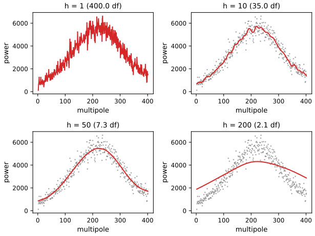
\[ \hr(x)=\sum_{i=1}^n\ell_i(x)Y_i, \tag{5.40} \] \[ \ell_i(x)=\frac{K\big(\frac{x-x_i}{h}\big)}{\sum_{j=1}^nK\big(\frac{x-x_j}{h}\big)}. \tag{5.41} \]The local average of Example 5.26 is the boxcar case (Remark 5.42). The kernel matters little; the bandwidth matters a lot (Example 5.43):
Theorem 5.44 (risk of the Nadaraya–Watson estimator) p. 73, (5.45)–(5.47)
Let \(x_1,\dots,x_n\) be drawn from a density \(f\). As \(h_n\to0\) and \(nh_n\to\infty\), the integrated risk is
\[ R(\hr,r)=\frac{h_n^4}{4}\Big(\int x^2K(x)\,\d x\Big)^2\int\Big(r''(x)+2r'(x)\frac{f'(x)}{f(x)}\Big)^2\d x+\frac{\sigma^2\int K^2(x)\,\d x}{nh_n}\int\frac{\d x}{f(x)}+o\Big(\frac1{nh_n}\Big)+o(h_n^4). \tag{5.45} \]The term
\[ 2r'(x)\frac{f'(x)}{f(x)} \tag{5.46} \]is the design bias. Minimising the two leading terms over \(h\) gives
\[ h_*=\Big(\frac1n\Big)^{1/5}\left(\frac{\sigma^2\int K^2(x)\,\d x\int\d x/f(x)}{\big(\int x^2K(x)\,\d x\big)^2\int\big(r''(x)+2r'(x)\frac{f'(x)}{f(x)}\big)^2\d x}\right)^{1/5}, \tag{5.47} \]so \(h_*=O(n^{-1/5})\) and the risk is \(O(n^{-4/5})\). (The book prints \(\int x^2K^2(x)\,\d x\) in the denominator of (5.47) and \(o(nh_n^{-1})\) in (5.45); the derivation below shows it must be \(\int x^2K(x)\,\d x\) and \(o((nh_n)^{-1})\): see Notes on the book.)
Filling the gap 5.6: where (5.45) comes from, pointwise and integrated p. 73
Assume: \(K\) is a symmetric density supported on \([-1,1]\) with \(\mu_2=\int u^2K\gt 0\); \(f\) is continuously differentiable and \(r\) twice continuously differentiable near \(x\), with \(f(x)\gt 0\); \(\V(\epsilon_i)=\sigma^2\); \(h\to0\), \(nh\to\infty\). Everything is conditional on the design, with the design then averaged by the law of large numbers.
Derivation
Ratio form. Put \(K_i=K((x_i-x)/h)\), \(\hat f(x)=(nh)^{-1}\sum_iK_i\) (a kernel density estimate) and \(\hat g(x)=(nh)^{-1}\sum_iK_i\{r(x_i)-r(x)\}\). Then, conditionally on the design,
\[ \E\hr(x)-r(x)=\frac{\hat g(x)}{\hat f(x)},\qquad \V\hr(x)=\sigma^2\frac{\sum_iK_i^2}{(\sum_iK_i)^2}=\frac{\sigma^2}{nh}\,\frac{(nh)^{-1}\sum_iK_i^2}{\hat f(x)^2}. \]The averages. Substituting \(x_i=x+hu\), for a random design
\[ \E\hat f(x)=\int K(u)f(x+hu)\,\d u=f(x)+O(h^2),\qquad \E\Big[\frac1{nh}\sum_iK_i^2\Big]=\int K^2(u)f(x+hu)\,\d u=f(x)R(K)+o(1), \] \[ \E\hat g(x)=\int K(u)\{r(x+hu)-r(x)\}f(x+hu)\,\d u. \]Expand \[ r(x+hu)-r(x)=hur'(x)+\tfrac12h^2u^2r''(x)+o(h^2) \] and \(f(x+hu)=f(x)+huf'(x)+o(h)\). Odd moments of \(K\) vanish, so
\[ \E\hat g(x)=h^2\mu_2\Big\{r'(x)f'(x)+\tfrac12r''(x)f(x)\Big\}+o(h^2). \]Each average has variance \(O((nh)^{-1})\) (its summands are bounded and supported on a window of probability \(O(h)\)), and \(\hat g\) has standard deviation \(O(h(nh)^{-1/2})=o(h^2)\) only when \(nh^3\to\infty\); in general the random part of \(\hat g\) is \(\OP(h(nh)^{-1/2})\), which is negligible next to the bias \(h^2\) at the optimal rate \(h\asymp n^{-1/5}\) (it is of order \(n^{-3/5}\) against \(n^{-2/5}\)). Dividing,
\[ \E\hr(x)-r(x)=h^2\mu_2\Big(\tfrac12r''(x)+\frac{r'(x)f'(x)}{f(x)}\Big)+\oP(h^2),\qquad \V\hr(x)=\frac{\sigma^2R(K)}{nhf(x)}\{1+\oP(1)\}, \]which are (5.67) and (5.66). Squaring the bias gives \(\tfrac{h^4}4\mu_2^2\big(r''+2r'f'/f\big)^2\); integrating squared bias and variance over \(x\) (assuming the remainders are uniform on the interval of integration, which excludes boundary regions of width \(h\)) gives (5.45).
The optimal bandwidth. Write the two leading terms as \(\tfrac14Ah^4+B/(nh)\) with \(A=\mu_2^2\int(r''+2r'f'/f)^2\) and \(B=\sigma^2R(K)\int\d x/f\). The derivative \(Ah^3-B/(nh^2)\) vanishes at \(h_*^5=B/(nA)\), which is (5.47) with \(\mu_2^2=(\int x^2K)^2\) in the denominator; the risk there is \(\tfrac54A^{1/5}B^{4/5}n^{-4/5}\). ∎
See also (companion course): Probability and Statistical Inference, Theorem 20.21 and Filling the gap 20.15, where the same derivation is done for the fixed design.
The design bias is a nuisance: the estimate of \(r\) depends on where the \(x\)'s happen to fall. The kernel estimator also has bias of order \(h\), not \(h^2\), within \(h\) of the ends of the data. Both are removed by local polynomials.
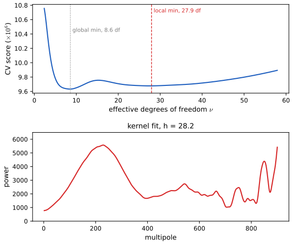
Example 5.48 chooses the bandwidth for all 899 CMB points by cross-validation:
Local polynomials. pp. 74–77 The kernel estimator minimises the locally weighted sum of squares \(\sum_iw_i(x)(Y_i-a)^2\) (5.49) with \(w_i(x)=K((x_i-x)/h)\): it fits a local constant. Fitting instead the polynomial
\[ P_x(u;a)=a_0+a_1(u-x)+\frac{a_2}{2!}(u-x)^2+\dots+\frac{a_p}{p!}(u-x)^p \tag{5.50} \]as an approximation \(r(u)\approx P_x(u;a)\) (5.51), one minimises
\[ \sum_{i=1}^nw_i(x)\big(Y_i-P_x(x_i;a)\big)^2 \tag{5.52} \]over \(a\) and sets
\[ \hr(x)=P_x(x;\hat a)=\hat a_0(x). \tag{5.53} \]In matrix form, with
\[ \bX_x=\begin{pmatrix}1&x_1-x&\cdots&\frac{(x_1-x)^p}{p!}\\ \vdots&\vdots&\ddots&\vdots\\ 1&x_n-x&\cdots&\frac{(x_n-x)^p}{p!}\end{pmatrix} \tag{5.54} \]and \(\bW_x=\diag(w_i(x))\), the criterion is \((\bY-\bX_xa)^\T\bW_x(\bY-\bX_xa)\) (5.55) and
\[ \hat a(x)=(\bX_x^\T\bW_x\bX_x)^{-1}\bX_x^\T\bW_x\bY. \tag{5.56} \]Theorem 5.57 (local polynomials are linear smoothers) p. 76
The local polynomial estimate is
\[ \hr(x)=\sum_{i=1}^n\ell_i(x)Y_i,\qquad \bl(x)^\T=e_1^\T(\bX_x^\T\bW_x\bX_x)^{-1}\bX_x^\T\bW_x, \tag{5.58} \]with \(e_1=(1,0,\dots,0)^\T\); it has mean \(\E\hr(x)=\sum_i\ell_i(x)r(x_i)\) and variance \(\V\hr(x)=\sigma^2\|\bl(x)\|^2\).
Proof
(5.55) is a weighted least squares criterion; when \(\bX_x^\T\bW_x\bX_x\) is invertible (at least \(p+1\) distinct \(x_i\) with positive weight), setting its gradient \(-2\bX_x^\T\bW_x(\bY-\bX_xa)\) to zero gives (5.56), the unique minimiser since the criterion is a convex quadratic with positive definite Hessian \(2\bX_x^\T\bW_x\bX_x\). \(\hat a_0=e_1^\T\hat a\) is (5.58). The weights do not involve \(\bY\), so \(\E\hr(x)=\bl(x)^\T\mathbf{r}\) and \(\V\hr(x)=\bl(x)^\T(\sigma^2\bI)\bl(x)\). ∎
The book's warning is worth repeating: although \(\hr(x)=\hat a_0(x)\), local linear regression is not a local constant fit; the slope term changes \(\hat a_0\) whenever the data around \(x\) are not symmetric about \(x\) (at a boundary, or with a non-uniform design). For \(p=1\) the weights have a closed form.
Theorem 5.60 (local linear weights) p. 77, (5.61)
For \(p=1\), \(\hr(x)=\sum_i\ell_i(x)Y_i\) with
\[ \ell_i(x)=\frac{b_i(x)}{\sum_{j=1}^nb_j(x)},\qquad b_i(x)=K\Big(\frac{x_i-x}{h}\Big)\big(S_{n,2}(x)-(x_i-x)S_{n,1}(x)\big), \tag{5.61} \]where \(S_{n,j}(x)=\sum_iK((x_i-x)/h)(x_i-x)^j\), \(j=1,2\).
Proof (Exercise 7)
Write \(K_i=K((x_i-x)/h)\), \(d_i=x_i-x\) and \(S_j=\sum_iK_id_i^j\) (so \(S_0=\sum_iK_i\)). With \(p=1\),
\[ \bX_x^\T\bW_x\bX_x=\begin{pmatrix}S_0&S_1\\S_1&S_2\end{pmatrix},\qquad (\bX_x^\T\bW_x\bX_x)^{-1}=\frac1{S_0S_2-S_1^2}\begin{pmatrix}S_2&-S_1\\-S_1&S_0\end{pmatrix}. \]The first row of the inverse times \(\bX_x^\T\bW_x\), whose \(i\)th column is \(K_i(1,d_i)^\T\), gives \(\ell_i=K_i(S_2-d_iS_1)/(S_0S_2-S_1^2)\). Finally \(\sum_jb_j=\sum_jK_j(S_2-d_jS_1)=S_0S_2-S_1^2\), the same denominator. The determinant is positive by Cauchy–Schwarz unless all \(x_i\) with \(K_i\gt 0\) coincide. ∎
In the code, local polynomials of any degree are computed from (5.58) (in the scaled variable \((x_i-x)/h\), for numerical stability) and the closed form (5.61) is used for speed; they agree to machine precision.
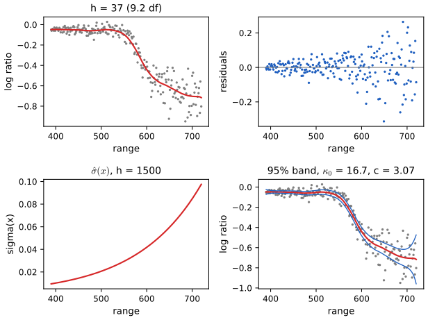
Example 5.59 applies local linear regression to the LIDAR data (221 laser measurements; the response is the log ratio of received light from two lasers, the covariate the distance travelled). Cross-validation over \(h\) gives \(h=37\) with \(\nu=9.19\), exactly the book's values, which confirms that the book used the tricube kernel.
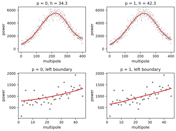
Example 5.62 compares \(p=0\) and \(p=1\) on the first 400 CMB points, each with its cross-validated bandwidth:
Example 5.63: the Doppler function
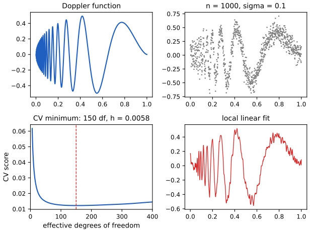
\[ r(x)=\sqrt{x(1-x)}\,\sin\Big(\frac{2.1\pi}{x+0.05}\Big),\qquad0\le x\le1, \tag{5.64} \]is spatially inhomogeneous: it oscillates ever faster as \(x\to0\). One bandwidth cannot suit both ends.
Theorem 5.65 (local linear against kernel regression; Fan 1992) pp. 79–80, (5.66)–(5.68)
Let \(Y_i=r(X_i)+\sigma(X_i)\epsilon_i\), \(a\le X_i\le b\), with \(X_1,\dots,X_n\) drawn from a density \(f\), and assume (i) \(f(x)\gt 0\), (ii) \(f\), \(r''\) and \(\sigma^2\) are continuous near \(x\), (iii) \(h_n\to0\), \(nh_n\to\infty\). For \(x\in(a,b)\), conditionally on the design, both estimators have variance
\[ \frac{\sigma^2(x)}{f(x)nh_n}\int K^2(u)\,\d u+\oP\Big(\frac1{nh_n}\Big). \tag{5.66} \]The Nadaraya–Watson estimator has bias
\[ h_n^2\Big(\frac12r''(x)+\frac{r'(x)f'(x)}{f(x)}\Big)\int u^2K(u)\,\d u+\oP(h^2), \tag{5.67} \]the local linear estimator
\[ h_n^2\,\frac12r''(x)\int u^2K(u)\,\d u+\oP(h^2). \tag{5.68} \]At the boundary points \(a\) and \(b\) the kernel estimator has bias of order \(h_n\) and the local linear estimator of order \(h_n^2\).
Filling the gap 5.7: why the slope removes the design bias and the boundary bias p. 80
Derivation
Exact reproduction of lines. With \(d_i=x_i-x\) and the weights (5.61), \(\sum_i\ell_i=1\) and
\[ \sum_i\ell_id_i=\frac{\sum_iK_id_i(S_2-d_iS_1)}{S_0S_2-S_1^2}=\frac{S_1S_2-S_2S_1}{S_0S_2-S_1^2}=0 . \](More generally a degree-\(p\) local polynomial reproduces polynomials of degree \(p\): Exercise 16.) Hence, by Taylor's theorem with \(r''\) continuous, the conditional bias is
\[ \sum_i\ell_i\{r(x_i)-r(x)-r'(x)d_i\}=\tfrac12r''(x)\sum_i\ell_id_i^2+o\Big(\sum_i|\ell_i|d_i^2\Big), \]and the first-order term \(r'(x)\sum_i\ell_id_i\), which is the source of the design bias for the kernel estimator, is identically zero.
The second moment of the weights. \(\sum_i\ell_id_i^2=(S_2^2-S_1S_3)/(S_0S_2-S_1^2)\). By the law of large numbers, as in Filling the gap 5.6, at an interior point \[ S_j=nh^{j+1}\{f(x)\mu_j+hf'(x)\mu_{j+1}+o_P(h)\} \] with \(\mu_j=\int u^jK\) (\(\mu_1=\mu_3=0\)). So \(S_0\approx nhf\), \(S_1\approx nh^3f'\mu_2\), \(S_2\approx nh^3f\mu_2\), \(S_3\approx nh^5f'\mu_4\), and
\[ \sum_i\ell_id_i^2=\frac{n^2h^6f^2\mu_2^2+O(n^2h^8)}{n^2h^4f^2\mu_2+O(n^2h^6)}=h^2\mu_2\{1+O_P(h^2)\}, \]which gives (5.68): no \(f'\). For the kernel estimator the first-order term survives: \(\sum_iK_id_i/\sum_iK_i=S_1/S_0\approx h^2\mu_2f'/f\), and \(r'(x)S_1/S_0\) is the design-bias part of (5.67).
Variance. \(\ell_i=K_i(S_2-d_iS_1)/(S_0S_2-S_1^2)\). On the window \(|d_i|\le h\), \[ |d_iS_1|/S_2\le h\cdot nh^3|f'|\mu_2/(nh^3f\mu_2)\{1+\oP(1)\}=O_P(h) \], and \(S_1^2/(S_0S_2)=O_P(h^2)\), so \(\ell_i=(K_i/S_0)\{1+O_P(h)\}\) uniformly in \(i\), and \[ \sum_i\sigma^2(x_i)\ell_i^2=\sigma^2(x)R(K)/(nhf(x))\{1+\oP(1)\} \], the same as for the kernel estimator: (5.66).
Boundary. At \(x=a\) only \(u=(x_i-a)/h\in[0,1]\) contributes, so the one-sided moments \(\mu_j^+=\int_0^1u^jK(u)\,\d u\) replace \(\mu_j\), and \(\mu_1^+\gt 0\). The kernel estimator's bias is \(r'(a)S_1/S_0+O(h^2)\approx r'(a)h\mu_1^+/\mu_0^+\): order \(h\). The local linear bias is still \(\tfrac12r''(a)\sum_i\ell_id_i^2\) (lines are reproduced exactly at any \(x\)), and
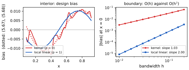
\[ \sum_i\ell_id_i^2\approx h^2\,\frac{(\mu_2^+)^2-\mu_1^+\mu_3^+}{\mu_0^+\mu_2^+-(\mu_1^+)^2}: \]order \(h^2\), with a larger constant than in the interior, and a variance also larger by a constant factor (the boundary equivalent kernel takes negative values). Figure 5.S1 confirms both claims on simulated designs: the exact conditional biases follow (5.67) and (5.68), and at \(x=0\) the bias decreases with slope 1.03 (kernel) and 2.00 (local linear) on the log–log scale. ∎
See also (companion course): Statistical Learning, Section 6.1.1 (local linear regression) and its local regression demo.
Remark 5.69: the result extends to degree \(p\); odd \(p\) removes design and boundary bias without increasing the asymptotic variance (going from \(p=2q\) to \(p=2q+1\) leaves the interior variance unchanged, because the extra odd moment is zero by symmetry). This is why local linear regression is the book's default.
5.5 Penalized Regression, Regularization and Splines
pp. 81–85 Instead of weighting the sum of squares locally, penalise roughness:
\[ M(\lambda)=\sum_i(Y_i-\hr(x_i))^2+\lambda J(r), \tag{5.70} \] \[ J(r)=\int(r''(x))^2\,\d x. \tag{5.71} \]\(\lambda=0\) allows any interpolating function; as \(\lambda\to\infty\) the solution tends to the least squares line (the only functions with \(J=0\)).
Definition 5.72 (splines) pp. 81–82
Given knots \(\xi_1\lt \dots\lt \xi_k\) in \((a,b)\), a cubic spline is a cubic polynomial on each interval between consecutive knots (and on the two outer intervals), with continuous first and second derivatives at the knots. An \(M\)th-order spline is piecewise of degree \(M-1\) with \(M-2\) continuous derivatives. A natural spline is linear beyond the boundary knots.
Theorem 5.73 (the smoothing spline) p. 82
The minimiser of \(M(\lambda)\) with penalty (5.71), over all functions with \(J(r)\lt \infty\), is a natural cubic spline with knots at the (distinct) data points: the smoothing spline.
Filling the gap 5.8: proof of Theorem 5.73 p. 82
Assume \(n\ge2\) distinct design points \(a\le x_1\lt \dots\lt x_n\le b\) (ties are handled by grouping) and work over the Sobolev space of functions on \([a,b]\) with absolutely continuous first derivative and \(\int r''^2\lt \infty\).
Proof
Step 1: interpolation. For any values \(z_1,\dots,z_n\) there is a natural cubic spline \(g\) with knots \(x_1,\dots,x_n\) and \(g(x_i)=z_i\). (Count: on the \(n-1\) inner intervals \(4(n-1)\) cubic coefficients; continuity of \(g,g',g''\) at the \(n-2\) interior knots imposes \(3(n-2)\) conditions, interpolation \(n\), natural end conditions \(g''(x_1)=g''(x_n)=0\) two more, a square linear system of size \(4n-4\); it is non-singular because, by Step 2 applied to \(z=0\), a solution with zero data has \(\int g''^2=0\), so \(g\) is a line vanishing at two points, hence zero.)
Step 2: the natural spline interpolant has the least roughness. Let \(\tilde g\) be any function in the space with \(\tilde g(x_i)=g(x_i)\), and \(\delta=\tilde g-g\), so \(\delta(x_i)=0\). Integrate by parts on each interval, using that \(g''\) is continuous, \(g''(x_1)=g''(x_n)=0\), and \(g'''\) is a constant \(c_i\) on \((x_i,x_{i+1})\):
\[ \int_a^bg''\delta''=\big[g''\delta'\big]_{x_1}^{x_n}-\int_{x_1}^{x_n}g'''\delta'=0-\sum_{i=1}^{n-1}c_i\{\delta(x_{i+1})-\delta(x_i)\}=0 \](outside \([x_1,x_n]\), \(g\) is linear so \(g''=0\) there). Hence \(\int\tilde g''^2=\int g''^2+\int\delta''^2\ge\int g''^2\), with equality iff \(\delta''\equiv0\), i.e. \(\delta\) is linear; vanishing at \(n\ge2\) points, \(\delta\equiv0\).
Step 3: conclusion. Let \(\tilde r\) be any candidate and \(g\) the natural spline interpolating \(\tilde r(x_1),\dots,\tilde r(x_n)\). The sums of squares in (5.70) are equal and \(J(g)\le J(\tilde r)\), so \(M(g)\le M(\tilde r)\), strictly unless \(\tilde r=g\). The problem therefore reduces to a minimisation over the \(n\)-dimensional space of natural cubic splines with knots at the data, where it is a strictly convex quadratic (Theorem 5.81) with a unique minimiser when \(\lambda\gt 0\). ∎
Theorem 5.74 (truncated power basis) p. 82, (5.75)
The functions \(h_1(x)=1\), \(h_2(x)=x\), \(h_3(x)=x^2\), \(h_4(x)=x^3\), \(h_j(x)=(x-\xi_{j-4})_+^3\) for \(j=5,\dots,k+4\) form a basis of the cubic splines with knots \(\xi_1,\dots,\xi_k\): every such spline is \(r(x)=\sum_{j=1}^{k+4}\beta_jh_j(x)\).
Proof
Each \(h_j\) is a cubic spline: \((x-\xi)_+^3\) is \(C^2\) with a jump of 6 in its third derivative at \(\xi\). Spanning: let \(r\) be a cubic spline; on \((-\infty,\xi_1)\) it equals a cubic \(q_0\). At \(\xi_1\), \(r-q_0\) is a cubic on \((\xi_1,\xi_2)\) vanishing with its first two derivatives at \(\xi_1\), so it equals \(\beta_5(x-\xi_1)^3\) there; hence \(r=q_0+\beta_5(x-\xi_1)_+^3\) up to \(\xi_2\), and induction over the knots gives \(r=q_0+\sum_j\beta_{j+4}(x-\xi_j)_+^3\). Independence: if \(\sum\beta_jh_j\equiv0\), the jump of the third derivative at \(\xi_j\) is \(6\beta_{j+4}=0\), and the remaining cubic is zero. So the dimension is \(k+4\). ∎
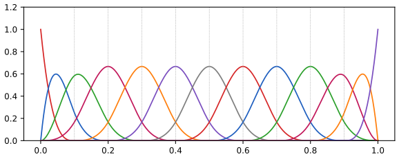
The truncated power basis is numerically poor (the columns are nearly collinear). The B-spline basis is better: with the augmented knots \(\tau_1\le\dots\le\tau_M\le\xi_0=a\), \(\tau_{j+M}=\xi_j\), \(b=\xi_{k+1}\le\tau_{k+M+1}\le\dots\le\tau_{k+2M}\) (usually the outer knots are all set to \(a\) and \(b\)), define \(B_{i,1}=I(\tau_i\le x\lt \tau_{i+1})\) and recursively
\[ B_{i,m}=\frac{x-\tau_i}{\tau_{i+m-1}-\tau_i}B_{i,m-1}+\frac{\tau_{i+m}-x}{\tau_{i+m}-\tau_{i+1}}B_{i+1,m-1},\qquad m\le M, \]with 0/0 read as 0 (the Cox–de Boor recursion).
Theorem 5.76 (B-spline basis) p. 83
\(\{B_{i,4}:i=1,\dots,k+4\}\) is a basis of the cubic splines with knots \(\xi_1,\dots,\xi_k\) on \([a,b]\).
Filling the gap 5.9: properties of B-splines, and why they form a basis p. 83
Derivation
By induction on \(m\), using the recursion: (a) support: \(B_{i,m}\) vanishes outside \([\tau_i,\tau_{i+m})\), since both terms involve functions supported there; (b) positivity: on its support the two coefficients \((x-\tau_i)/(\tau_{i+m-1}-\tau_i)\) and \((\tau_{i+m}-x)/(\tau_{i+m}-\tau_{i+1})\) are non-negative where the corresponding lower-order function is non-zero; (c) partition of unity on \([a,b]\): \(\sum_iB_{i,m}(x)=1\). For (c), collect the coefficient of \(B_{i,m-1}\) in \(\sum_iB_{i,m}\): it comes from the first term of \(B_{i,m}\) and the second term of \(B_{i-1,m}\), and these coefficients add to \(\frac{x-\tau_i}{\tau_{i+m-1}-\tau_i}+\frac{\tau_{i+m-1}-x}{\tau_{i+m-1}-\tau_i}=1\); so \[ \sum_iB_{i,m}=\sum_iB_{i,m-1}=\dots=\sum_iB_{i,1}=1 \]. (d) smoothness: \(B_{i,M}\) is a piecewise polynomial of degree \(M-1\) and, at a simple knot, has \(M-2\) continuous derivatives (by the derivative formula \[ B_{i,m}'=(m-1)\{B_{i,m-1}/(\tau_{i+m-1}-\tau_i)-B_{i+1,m-1}/(\tau_{i+m}-\tau_{i+1})\} \], induction raises the smoothness by one at each order).
Basis. By (d) each \(B_{i,4}\) is a cubic spline with the given knots, and there are \(k+4\) of them, the dimension found in Theorem 5.74; so it suffices to show that they span the spline space, and independence follows by counting. Spanning follows from Marsden's identity (proved by induction on the order with the recursion): for every real \(y\), \((x-y)^{3}=\sum_i\psi_i(y)B_{i,4}(x)\) on \([a,b]\) with \(\psi_i(y)=(\tau_{i+1}-y)(\tau_{i+2}-y)(\tau_{i+3}-y)\). Taking derivatives in \(y\) shows that \(1,x,x^2,x^3\) are combinations of B-splines; and keeping only the terms with \(\tau_{i}\ge\xi_j\) (the B-splines supported to the right of \(\xi_j\)) gives \((x-\xi_j)_+^3\) as a combination, because those B-splines vanish left of \(\xi_j\) and reproduce \((x-\xi_j)^3\) to the right of it. So the B-splines span the truncated power basis of Theorem 5.74 (Curry and Schoenberg 1966; de Boor 2001, Chapter IX). The implementation of the recursion in the code agrees with scipy's B-splines to \(2\times10^{-16}\), and the rows of the basis sum to one. ∎
By Theorem 5.73 the smoothing spline can be written
\[ \hr(x)=\sum_{j=1}^N\hat\beta_jB_j(x), \tag{5.77} \]with B-splines on knots at the data (\(N=\) number of distinct interior design points \(+4\); the natural boundary conditions need not be imposed, the minimiser satisfies them automatically by Theorem 5.73). The criterion becomes
\[ (\bY-\bB\beta)^\T(\bY-\bB\beta)+\lambda\beta^\T\Omega\beta, \tag{5.78} \]with \(B_{ij}=B_j(x_i)\) and \(\Omega_{jk}=\int B_j''(x)B_k''(x)\,\d x\).
Theorems 5.79 and 5.81 (the smoothing spline is a linear smoother) p. 84, (5.80), (5.82), (5.83)
\[ \hat\beta=(\bB^\T\bB+\lambda\Omega)^{-1}\bB^\T\bY, \tag{5.80} \] \[ \mathbf{L}=\bB(\bB^\T\bB+\lambda\Omega)^{-1}\bB^\T, \tag{5.82} \] \[ \hat{\mathbf{r}}=\mathbf{L}\bY. \tag{5.83} \]Filling the gap 5.10: the solution, its shrinkage form, the degrees of freedom, and exact leave-one-out p. 84
Derivation
Solution. \(\Omega\) is positive semidefinite (\(\beta^\T\Omega\beta=\int(\sum\beta_jB_j'')^2\ge0\)); its null space is the coefficients of lines. The criterion (5.78) has gradient \(-2\bB^\T(\bY-\bB\beta)+2\lambda\Omega\beta\) and Hessian \(2(\bB^\T\bB+\lambda\Omega)\), which is positive definite for \(\lambda\gt 0\) as soon as no non-zero spline is both zero at all data points and a line, i.e. with at least two distinct \(x_i\). Setting the gradient to zero gives (5.80), and (5.82)–(5.83) follow, with \(\mathbf{L}\) not depending on \(\bY\).
Shrinkage (Demmler–Reinsch) form. With a full-rank \(\bB\) (knots at the data, \(N=n\) for natural splines), simultaneously diagonalise: there is an orthonormal basis \(u_1,\dots,u_n\) of \(\R^n\) and \(0=d_1=d_2\lt d_3\le\dots\le d_n\) such that
\[ \mathbf{L}=\sum_{k=1}^n\frac1{1+\lambda d_k}u_ku_k^\T,\qquad \nu=\tr\mathbf{L}=\sum_{k=1}^n\frac1{1+\lambda d_k}. \](Write \(\mathbf{L}=(\bI+\lambda\mathbf{K})^{-1}\) with \(\mathbf{K}=\bB^{-\T}\Omega\bB^{-1}\) symmetric positive semidefinite, and take its eigen-decomposition; the two zero eigenvalues are the constant and linear vectors.) So the smoothing spline keeps the two "line" components of \(\bY\), and shrinks the component along \(u_k\) by \(1/(1+\lambda d_k)\), the more the rougher \(u_k\) is. Consequences: \(\mathbf{L}\) is symmetric with eigenvalues in \((0,1]\), \(\nu\) decreases strictly and continuously from \(n\) (\(\lambda=0\), interpolation) to 2 (\(\lambda\to\infty\), the least squares line). Footnote 5 of the book: (5.80) is a generalised ridge regression, ordinary ridge when \(\Omega=\bI\). In the code \(\lambda\) is found from a target \(\nu\) by solving \(\tr\mathbf{L}(\lambda)=\nu\), which this monotonicity makes well posed.
Exact leave-one-out. Let \(\hat r_{(-i)}\) minimise the criterion without observation \(i\), and set \(Y^*_j=Y_j\) for \(j\ne i\), \(Y^*_i=\hat r_{(-i)}(x_i)\). For any \(g\), \[ M^*(g)=\sum_{j\ne i}(Y_j-g(x_j))^2+(Y_i^*-g(x_i))^2+\lambda J(g)\ge\sum_{j\ne i}(Y_j-g(x_j))^2+\lambda J(g)\ge \] the value of that criterion at \(\hat r_{(-i)}\), which equals \(M^*(\hat r_{(-i)})\). So \(\hat r_{(-i)}\) minimises \(M^*\), whose minimiser is \(\mathbf{L}\bY^*\) (same \(\mathbf{L}\): the knots are all the \(x\)'s in both problems). Its \(i\)th coordinate gives \(\hat r_{(-i)}(x_i)=\hr(x_i)-L_{ii}Y_i+L_{ii}\hat r_{(-i)}(x_i)\), i.e. \(Y_i-\hat r_{(-i)}(x_i)=(Y_i-\hr(x_i))/(1-L_{ii})\): Theorem 5.34 holds for the smoothing spline with the true refit, not merely with the definition (5.32). ∎
The implementation (B-spline recursion, \(\Omega\) by two-point Gauss–Legendre quadrature on each knot interval, exact because \(B_j''\) is linear there) reproduces scipy's smoothing spline to \(10^{-9}\).
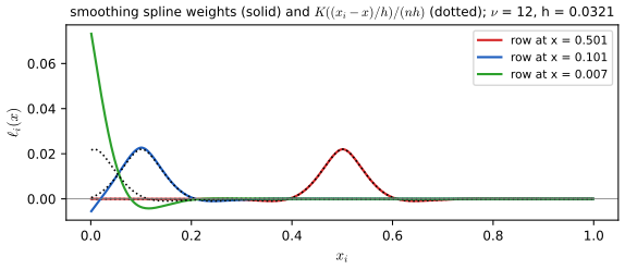
Silverman (1984) showed that the smoothing spline is approximately a kernel smoother with a bandwidth that adapts to the design density:
Filling the gap 5.11: Silverman's equivalent kernel, with the factor \(1/n\) p. 84
Claim (for the criterion (5.70) with a design of density \(f\), away from the boundary): \(\ell_i(x)\approx\dfrac1{n f(x_i)h(x_i)}K\Big(\dfrac{x_i-x}{h(x_i)}\Big)\), \(h(x)=\Big(\dfrac{\lambda}{nf(x)}\Big)^{1/4}\), \(K(t)=\tfrac12e^{-|t|/\sqrt2}\sin\big(|t|/\sqrt2+\pi/4\big)\). The book's display omits the factor \(1/n\).
Derivation (continuous approximation)
Replace the sum of squares by its continuous version: \[ \sum_i(Y_i-g(x_i))^2\approx n\int(y(t)-g(t))^2f(t)\,\d t \] for a "signal" \(y\). The Euler–Lagrange equation of \(n\int(y-g)^2f+\lambda\int g''^2\) is \(\lambda g''''(t)+nf(t)\{g(t)-y(t)\}=0\). Freeze \(f\) near \(t\) at \(f(t)\) and set \(h^4=\lambda/(nf)\): \(h^4g''''+g=y\). Its Green's function on the line is the inverse Fourier transform of \(1/(1+h^4\omega^4)\), which is \(h^{-1}K(s/h)\) with the \(K\) above (check: \(\int K=1\), and \(K\) is even, decays exponentially and has side lobes of negative weight). So \(g(t)=\int h^{-1}K((s-t)/h)y(s)\,\d s\). Discretising \(\int\phi(s)y(s)\,\d s\approx\sum_iy(x_i)\phi(x_i)/(nf(x_i))\), because the design points have density \(nf\), gives \(\ell_i(t)\approx K((x_i-t)/h)/(nf(x_i)h)\). The sum over \(i\) of these weights is about \(\int h^{-1}K=1\) only with the \(1/n\): without it the weights would sum to \(n\). Rigorous versions with error bounds are in Silverman (1984) and Nychka (1995). Figure 5.S2 compares rows of the exact \(\mathbf{L}\) with this approximation. ∎
Regression splines. With few knots and no penalty, \(\hat{\mathbf{r}}=\mathbf{L}\bY\) with \(\mathbf{L}=\bB(\bB^\T\bB)^{-1}\bB^\T\), a projection with \(\nu=\) the number of basis functions; the smoothness is set by the number and placement of the knots (Ruppert, Wand and Carroll 2003). Exercise 11 chooses the number of knots by cross-validation for the motorcycle data.
See also (companion courses): Statistical Learning, Section 5.4 (smoothing splines) with its smoothing spline demo and regression splines demo; Applied Statistical Learning, Section 7.5.
5.6 Variance Estimation
Theorem 5.85 (variance estimate for a linear smoother) pp. 85–86, (5.86)
Let \(\hr\) be a linear smoother with smoothing matrix \(\mathbf{L}\) and
\[ \hs^2=\frac{\sum_{i=1}^n(Y_i-\hr(x_i))^2}{n-2\nu+\tilde\nu},\qquad \nu=\tr(\mathbf{L}),\quad \tilde\nu=\tr(\mathbf{L}^\T\mathbf{L})=\sum_{i=1}^n\|\bl(x_i)\|^2. \tag{5.86} \]If \(r\) is sufficiently smooth, \(\nu=o(n)\) and \(\tilde\nu=o(n)\), then \(\hs^2\) is consistent for \(\sigma^2\). (The book's numerator has \(r(x_i)\), a misprint for \(\hr(x_i)\).)
The book outlines the proof with the quadratic form identity
\[ \E(\bY^\T Q\bY)=\tr(QV)+\mu^\T Q\mu \tag{5.87} \](\(V=\V\bY\), \(\mu=\E\bY\)) and \(\hs^2=\bY^\T\Lambda\bY/\tr\Lambda\) (5.88) with \(\Lambda=(\bI-\mathbf{L})^\T(\bI-\mathbf{L})\), and stops at "one can show that \(\V(\hs^2)\to0\)". Here is the whole argument (Exercise 8).
Filling the gap 5.12: (5.87), the bias of \(\hs^2\), and conditions for consistency p. 86
Proof
(5.87). \(\bY^\T Q\bY\) is a scalar, so it equals its trace: \[ \E\tr(Q\bY\bY^\T)=\tr(Q\,\E\bY\bY^\T)=\tr\{Q(V+\mu\mu^\T)\}=\tr(QV)+\mu^\T Q\mu \]. No distributional assumption is needed.
Mean. \(\bY-\hat{\mathbf{r}}=(\bI-\mathbf{L})\bY\), so \(\sum_i(Y_i-\hr(x_i))^2=\bY^\T\Lambda\bY\) and \[ \tr\Lambda=\tr(\bI-\mathbf{L}-\mathbf{L}^\T+\mathbf{L}^\T\mathbf{L})=n-2\nu+\tilde\nu \]. With \(V=\sigma^2\bI\) and \(\mu=\mathbf{r}\), (5.87) gives
\[ \E\hs^2=\sigma^2+\frac{\mathbf{r}^\T\Lambda\mathbf{r}}{n-2\nu+\tilde\nu}=\sigma^2+\frac{\|(\bI-\mathbf{L})\mathbf{r}\|^2}{n-2\nu+\tilde\nu}. \]The bias term is \(n/(n-2\nu+\tilde\nu)\) times the average squared bias of the fitted values, \(n^{-1}\|\mathbf{r}-\mathbf{L}\mathbf{r}\|^2\), which tends to 0 whenever the smoother is consistent at the design points (for a kernel or local linear smoother with \(h\to0\) and \(r\) twice differentiable it is \(O(h^4)\), plus \(O(h/n\cdot n)\cdot O(h^2)\)-type boundary contributions, which are \(O(h^3)\)). The denominator is \(n(1+o(1))\) when \(\nu,\tilde\nu=o(n)\).
Variance. Assume in addition \(\E\epsilon_i^4\lt \infty\). For a symmetric \(Q\) and \(\bY=\mu+\epsilon\) with independent errors, \[ \V(\bY^\T Q\bY)=\V(\epsilon^\T Q\epsilon)+4\mu^\T QVQ\mu+4\E(\epsilon^\T Q\epsilon\,\epsilon^\T Q\mu) \], and the standard computation gives
\[ \V(\epsilon^\T Q\epsilon)=2\sigma^4\tr(Q^2)+(\E\epsilon^4-3\sigma^4)\sum_iQ_{ii}^2,\qquad |\E(\epsilon^\T Q\epsilon\,\epsilon^\T Q\mu)|\le|\E\epsilon^3|\sum_i|Q_{ii}||(Q\mu)_i|. \]For \(Q=\Lambda\): \(\Lambda\) is positive semidefinite with \(\|\Lambda\|_{\rm op}\le\|\bI-\mathbf{L}\|_{\rm op}^2\). If the operator norm of \(\mathbf{L}\) is bounded (true for kernel, local polynomial and spline smoothers with bounded effective kernels: \(\|\mathbf{L}\|_{\rm op}\le\max_i\sum_j|L_{ij}|\) and \(\max_j\sum_i|L_{ij}|\) bounded), then \(\tr\Lambda^2\le\|\Lambda\|_{\rm op}\tr\Lambda=O(n)\), \(\sum_i\Lambda_{ii}^2=O(n)\), and \(\mu^\T\Lambda^2\mu\le\|\Lambda\|_{\rm op}\|(\bI-\mathbf{L})\mathbf{r}\|^2=o(n)\). Hence \(\V(\bY^\T\Lambda\bY)=O(n)\) and \[ \V(\hs^2)=O(n)/(n-2\nu+\tilde\nu)^2=O(1/n)\to0 \].
Conclusion. Sufficient conditions: \(\E\epsilon^4\lt \infty\); \(\nu=o(n)\) and \(\tilde\nu=o(n)\); \(\|\mathbf{L}\|_{\rm op}=O(1)\); and \(n^{-1}\|(\bI-\mathbf{L})\mathbf{r}\|^2\to0\). Then \(\E\hs^2\to\sigma^2\) and \(\V\hs^2\to0\), so \(\hs^2\to\sigma^2\) in probability by Chebyshev's inequality. If \(\mathbf{L}\) is a projection of rank \(p\) (regression splines), \(\nu=\tilde\nu=p\) and (5.86) reduces to (5.11); if moreover \(\mathbf{r}\) is in the column space, \(\hs^2\) is exactly unbiased. ∎
Two difference-based estimators avoid choosing a smoother at all. Rice (1984), with the \(x_i\) sorted:
\[ \hs^2=\frac1{2(n-1)}\sum_{i=1}^{n-1}(Y_{i+1}-Y_i)^2, \tag{5.89} \]motivated by \(\E(Y_{i+1}-Y_i)^2\approx\E(\epsilon_{i+1}^2)+\E(\epsilon_i^2)=2\sigma^2\) (5.90). Gasser, Sroka and Jennen-Steinmetz (1986):
\[ \hs^2=\frac1{n-2}\sum_{i=2}^{n-1}c_i^2\delta_i^2, \tag{5.91} \]with \(\delta_i=a_iY_{i-1}+b_iY_{i+1}-Y_i\), \(a_i=(x_{i+1}-x_i)/(x_{i+1}-x_{i-1})\), \(b_i=(x_i-x_{i-1})/(x_{i+1}-x_{i-1})\), \(c_i^2=(a_i^2+b_i^2+1)^{-1}\).
Filling the gap 5.13: the difference estimators are consistent, and Gasser's is exact for lines (Exercise 5) pp. 86–87
Proof
Rice. Assume \(r\) is Lipschitz with constant \(M\) on \([a,b]\), the design is sorted, and the errors are iid with variance \(\sigma^2\) and \(\E\epsilon^4\lt \infty\). With \(\Delta_i=r(x_{i+1})-r(x_i)\), \(Y_{i+1}-Y_i=\Delta_i+\epsilon_{i+1}-\epsilon_i\) and
\[ \E\hs^2=\sigma^2+\frac1{2(n-1)}\sum_i\Delta_i^2,\qquad 0\le\frac1{2(n-1)}\sum_i\Delta_i^2\le\frac{M^2}{2(n-1)}\sum_i(x_{i+1}-x_i)^2\le\frac{M^2(b-a)}{2(n-1)}\max_i(x_{i+1}-x_i). \]For an equispaced design the bias is \(O(n^{-2})\). For the variance, the terms \(D_i=(Y_{i+1}-Y_i)^2\) are 1-dependent (\(D_i\) and \(D_j\) are independent when \(|i-j|\ge2\)), so \(\V(\sum_iD_i)\le3\sum_i\V(D_i)=O(n)\) and \(\V\hs^2=O(1/n)\). Hence \(\hs^2\to\sigma^2\) in probability. For Normal errors and constant \(r\) the variance is exact: \(U_i=\epsilon_{i+1}-\epsilon_i\sim N(0,2\sigma^2)\), so \(\V(D_i)=2(2\sigma^2)^2=8\sigma^4\); consecutive differences have covariance \(-\sigma^2\), and for jointly Normal variables \(\Cov(U^2,V^2)=2\Cov(U,V)^2\), so \(\Cov(D_i,D_{i+1})=2\sigma^4\). Hence \(\V\sum_iD_i=8(n-1)\sigma^4+4(n-2)\sigma^4\) and
\[ \V\hs^2=\frac{(3n-5)\sigma^4}{(n-1)^2}\approx\frac{3\sigma^4}{n}, \]1.5 times the variance \(2\sigma^4/n\) of the oracle \(n^{-1}\sum_i\epsilon_i^2\): differencing loses a constant factor, not the rate.
Gasser et al. If \(r\) is linear on \([x_{i-1},x_{i+1}]\), then \(a_ir(x_{i-1})+b_ir(x_{i+1})=r(x_i)\), because \(a_i+b_i=1\) and \(a_ix_{i-1}+b_ix_{i+1}=x_i\) (the line through the outer two points evaluated at the middle one). Then \(\delta_i=a_i\epsilon_{i-1}+b_i\epsilon_{i+1}-\epsilon_i\) has mean 0 and variance \(\sigma^2(a_i^2+b_i^2+1)\), so \(c_i^2\delta_i^2\) is exactly unbiased for \(\sigma^2\): the estimator is unbiased for every linear \(r\) and any design. For smooth \(r\) the bias of \(c_i^2\delta_i^2\) is \(O((x_{i+1}-x_{i-1})^4)\), and the terms are 2-dependent, so the same argument gives consistency. ∎
See also (companion course): Probability and Statistical Inference, Filling the gap 20.17 (the bias of the difference estimator).
Example 5.92, on the first 400 CMB points with the local linear fit: (5.86) gives \(\hs^2=168{,}374\), i.e. \(\hs=410.3\); Rice's (5.89) gives \(\hs^2=155{,}670\), \(\hs=394.55\); Gasser's gives \(\hs^2=151{,}554\). The book reports 408.29 and 394.55: these are standard deviations, not variances (Notes on the book).
Heteroscedasticity. pp. 87–89 In the model
\[ Y_i=r(x_i)+\sigma(x_i)\epsilon_i \tag{5.93} \]put \(Z_i=\log(Y_i-r(x_i))^2\) and \(\delta_i=\log\epsilon_i^2\); then
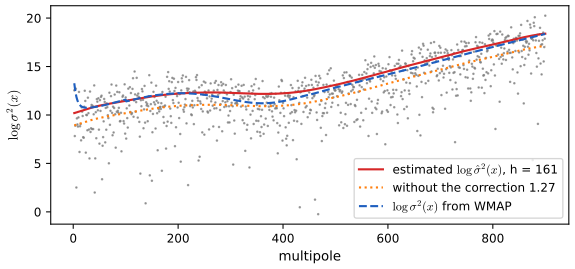
\[ Z_i=\log\big(\sigma^2(x_i)\big)+\delta_i. \tag{5.94} \]The book's recipe: (1) fit \(\hr\); (2) set \(Z_i=\log(Y_i-\hr(x_i))^2\); (3) smooth the \(Z_i\) against \(x_i\) to get \(\hat q(x)\) and set
\[ \hs^2(x)=e^{\hat q(x)}. \tag{5.95} \]Filling the gap 5.14: the log-residual recipe estimates \(0.28\,\sigma^2(x)\) unless corrected pp. 87–88
Derivation
The regression of \(Z_i\) on \(x_i\) estimates \(\E Z_i=\log\sigma^2(x_i)+\E\delta_i\), and \(\E\delta_i=\E\log\epsilon^2\) is not 0. For \(\epsilon\sim N(0,1)\), \(\epsilon^2\sim\chi^2_1=\mathrm{Gamma}(\tfrac12,2)\), and for \(W\sim\mathrm{Gamma}(k,\theta)\), \(\E\log W=\psi(k)+\log\theta\) (differentiate \(\int w^{k-1}e^{-w/\theta}\d w=\Gamma(k)\theta^k\) in \(k\)). So
\[ \E\log\epsilon^2=\psi(\tfrac12)+\log2=-\gamma-2\log2+\log2=-\gamma-\log2=-1.2704, \]with \(\gamma\) Euler's constant. The recipe as stated therefore estimates \(\log\sigma^2(x)-1.27\), i.e. \(e^{-1.27}\sigma^2(x)=0.28\,\sigma^2(x)\): the standard deviation is underestimated by a factor \(0.53\), and a band built on it is about half as wide as it should be. The fix is to add \(1.2704\) to \(\hat q\) (for Normal errors), or, without assuming normality, to rescale so that \(n^{-1}\sum_i(Y_i-\hr(x_i))^2/\hs^2(x_i)=1\). The code adds 1.2704. Figure 5.9 is the evidence: for the CMB data the WMAP team's independent \(\sigma^2(x)\) is available, and the corrected estimate follows it (on average 0.28 above it on the log scale, part of which is the residuals' own extra variability) while the uncorrected one lies on average 0.99 below it. (The residuals \(Y_i-\hr(x_i)\) also have variance \(\sigma^2(x_i)(1-2L_{ii}+\sum_jL_{ij}^2)\) rather than \(\sigma^2(x_i)\); for the bandwidths used here the factor is within a few percent of 1.)
Two further remarks of the book: a very small residual gives a large negative \(Z_i\), an outlier, so smoothing the squared residuals directly (a non-Gaussian regression, Section 5.10) is an alternative; and the method works with any smoother in both steps. ∎
5.7 Confidence Bands
pp. 89–94 Bands will be of the form
\[ \hr(x)\pm c\,\widehat{\se}(x). \tag{5.97} \]The bias problem. With \(\br(x)=\E\hr(x)\) and \(s_n(x)\) the standard deviation of \(\hr(x)\),
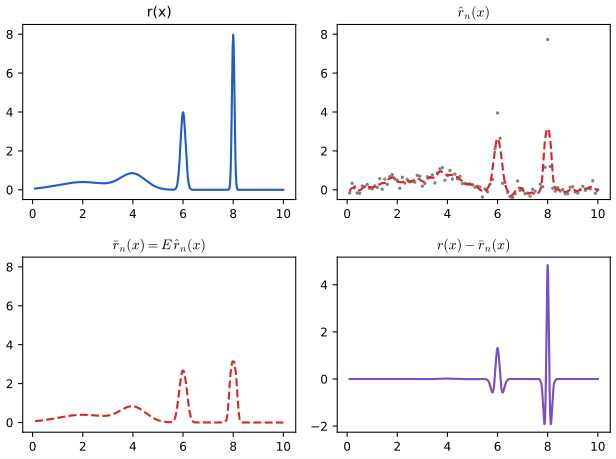
\[ \frac{\hr(x)-r(x)}{s_n(x)}=\underbrace{\frac{\hr(x)-\br(x)}{s_n(x)}}_{Z_n(x)}+\frac{\mathrm{bias}(\hr(x))}{\sqrt{\mathrm{variance}(\hr(x))}}. \]The first term is asymptotically \(N(0,1)\); the second does not vanish when \(h\) is chosen to balance bias and variance. So a band of the form (5.97) is a band for \(\br\), the smoothed version of \(r\), not for \(r\).
Filling the gap 5.15: how large the bias term is, and what undersmoothing buys pp. 89–90
Derivation
At an interior point the local linear estimator has bias \(b(x)h^2\) with \(b=\tfrac12\mu_2r''(x)\) and variance \(v(x)/(nh)\) with \(v=\sigma^2R(K)/f(x)\) (Theorem 5.65). The pointwise mean squared error \(b^2h^4+v/(nh)\) is minimised at \(h_x^5=v/(4b^2n)\), where \(b^2h^4=\tfrac14v/(nh)\): the squared bias is one quarter of the variance, so
\[ \frac{\text{bias}}{\text{sd}}=\frac12\sgn(r''(x))\quad\text{at the pointwise optimal }h, \]for every \(n\). A nominal 95 percent pointwise interval \(\hr(x)\pm1.96\,s_n(x)\) then covers \(r(x)\) with probability \[ \P(|Z+\tfrac12|\le1.96)=\Phi(1.46)-\Phi(-2.46)=0.921 \], not 0.95, forever. With a global bandwidth, the ratio is \(\tfrac12\) on average and larger where \(|r''|\) is large: at the peaks of Example 5.98 the bias dominates. Undersmoothing: with \(h=o(n^{-1/5})\), \(\text{bias}/\text{sd}\asymp h^2\sqrt{nh}=\sqrt{nh^5}\to0\), and the band becomes a band for \(r\); the price is a width of order \((nh)^{-1/2}\gg n^{-2/5}\). The coverage error rates (5.152)–(5.155) of Section 5.13 quantify this. Figure 5.S3 shows it by simulation. ∎
Example 5.98 makes the point with
\[ r(x)=\phi(x;2,1)+\phi(x;4,0.5)+\phi(x;6,0.1)+\phi(x;8,0.05), \]where \(\phi(x;m,s)\) is the Normal density with mean \(m\) and standard deviation \(s\) (the book says "variance \(s^2\)", consistent), observed as \(Y_i=r(i/10)+0.2\,\epsilon_i\), \(i=1,\dots,100\), smoothed by local linear regression with \(h=0.27\).
Constructing bands. For a linear smoother, \(\br(x)=\sum_i\ell_i(x)r(x_i)\) and, with constant variance, \(\V\hr(x)=\sigma^2\|\bl(x)\|^2\). Consider
\[ I(x)=\big(\hr(x)-c\,\hs\|\bl(x)\|,\ \hr(x)+c\,\hs\|\bl(x)\|\big),\qquad a\le x\le b. \tag{5.99} \]For known \(\sigma\) and Normal errors (Sun and Loader 1994),
\[ \P\big(\br(x)\notin I(x)\text{ for some }x\in[a,b]\big)=\P\Big(\max_{x\in[a,b]}\frac{|\sum_i\epsilon_i\ell_i(x)|}{\sigma\|\bl(x)\|}\gt c\Big)=\P\Big(\max_{x\in[a,b]}|W(x)|\gt c\Big), \]where \(W(x)=\sum_iZ_iT_i(x)\), \(Z_i=\epsilon_i/\sigma\sim N(0,1)\) and \(T(x)=\bl(x)/\|\bl(x)\|\) is a unit vector. \(W\) is a Gaussian process with unit variance, and
\[ \P\Big(\max_x\Big|\sum_{i=1}^nZ_iT_i(x)\Big|\gt c\Big)\approx2(1-\Phi(c))+\frac{\kappa_0}{\pi}e^{-c^2/2} \tag{5.100} \]for large \(c\), where
\[ \kappa_0=\int_a^b\|T'(x)\|\,\d x \tag{5.101} \]is the length of the curve \(x\mapsto T(x)\) on the unit sphere. Choosing \(c\) to solve
\[ 2(1-\Phi(c))+\frac{\kappa_0}{\pi}e^{-c^2/2}=\alpha \tag{5.102} \]gives the simultaneous band. With \(\sigma\) estimated, Sun and Loader replace the right side of (5.100) by \(\P(|T_m|\gt c)+\frac{\kappa_0}{\pi}(1+c^2/m)^{-m/2}\), \(T_m\sim t_m\), \(m=n-\tr\mathbf{L}\).
Filling the gap 5.16: the tube formula from Rice's formula, and the approximation of Exercise 20 pp. 91–92, (5.100)–(5.102)
Derivation
Setting. \(W(x)=\langle Z,T(x)\rangle\) with \(\|T(x)\|=1\), so \(\V W(x)=1\), and differentiating \(\|T\|^2=1\) gives \(\langle T,T'\rangle=0\): \(W(x)\) and \(W'(x)=\langle Z,T'(x)\rangle\) are uncorrelated, hence independent (jointly Normal), with \(\V W'(x)=\|T'(x)\|^2\).
Rice's formula (Rice 1944; Cramér and Leadbetter 1967, Chapter 10): for a smooth Gaussian process the expected number of upcrossings of the level \(c\) on \([a,b]\) is
\[ \E N_c^+=\int_a^b\int_0^\infty y\,p_x(c,y)\,\d y\,\d x, \]with \(p_x\) the joint density of \((W(x),W'(x))\), equation (5.156). By independence \(p_x(c,y)=\phi(c)\,\|T'\|^{-1}\phi(y/\|T'\|)\), and \(\int_0^\infty y\,\phi(y/s)/s\,\d y=s/\sqrt{2\pi}\). So
\[ \E N_c^+=\phi(c)\int_a^b\frac{\|T'(x)\|}{\sqrt{2\pi}}\,\d x=\frac{\kappa_0}{2\pi}e^{-c^2/2}. \]Bound. \[ \{\sup_xW(x)\gt c\}\subset\{W(a)\gt c\}\cup\{N_c^+\ge1\} \], so \(\P(\sup W\gt c)\le1-\Phi(c)+\E N_c^+\) (Markov's inequality for the integer \(N_c^+\)). The same for \(-W\) (downcrossings of \(-c\)) and a union bound give
\[ \P\Big(\sup_x|W(x)|\gt c\Big)\le2(1-\Phi(c))+\frac{\kappa_0}{\pi}e^{-c^2/2}, \]which is (5.100) as an inequality. It is also sharp for large \(c\): \(\P(N_c^+\ge2)\) and the overlap of the events are of smaller order, \(o(e^{-c^2/2})\) (Adler and Taylor 2007, Chapter 14). Since the bound is conservative, solving (5.102) gives a band whose coverage is at least \(1-\alpha\) (exactly so for Normal errors and known \(\sigma\)). Hotelling's (1939) and Naiman's (1990) volume-of-tubes argument in the Appendix gives the same leading terms.
Computing \(\kappa_0\). In the code \(T(x)\) is evaluated on a fine grid, differentiated by central differences, and \(\|T'\|\) integrated by the trapezoid rule; the grid of 600 to 1500 points is fine enough that \(\kappa_0\) changes by less than 0.1 percent when it is doubled.
Exercise 20. If \(\ell_i(x)\propto K((x-x_i)/h)\) with equispaced \(x_i\) and no boundary effects, then (the normalisation of \(\ell\) cancels in \(T\)) \(T_i=K_i/\|K_\cdot\|\) with \(K_i=K((x-x_i)/h)\) and \[ T_i'=K_i'/(h\|K_\cdot\|)-K_i\langle K_\cdot,K'_\cdot\rangle/(h\|K_\cdot\|^3) \]. The sums are Riemann sums: \(\sum_iK_i^2\approx(n/(b-a))h\int K^2\), \(\sum_iK_i'^2\approx(n/(b-a))h\int K'^2\), \(\sum_iK_iK_i'\approx(n/(b-a))h\int KK'=0\) (\(KK'=(K^2)'/2\) integrates to 0). Hence \(\|T'(x)\|\approx h^{-1}\|K'\|/\|K\|\) and
\[ \kappa_0\approx\frac{b-a}{h}\,\frac{\|K'\|}{\|K\|},\qquad\|g\|^2=\int g^2. \]For the tricube kernel \(\|K'\|/\|K\|=1.78\) (computed numerically). For the LIDAR data (\(b-a=330\), \(h=37\)) this gives \(\kappa_0\approx15.9\); the exact value is 15.3 for the kernel smoother and 16.7 for the local linear smoother, whose boundary weights add length; the book's \(\kappa_0\approx30\) is inconsistent with both (Notes on the book). ∎
Non-constant variance. If \(\sigma(x)\) varies, \(\V\hr(x)=\sum_i\sigma^2(x_i)\ell_i^2(x)\), and the band is
\[ I(x)=\hr(x)\pm c\,s(x),\qquad s(x)=\Big(\sum_{i=1}^n\hs^2(x_i)\ell_i^2(x)\Big)^{1/2}, \tag{5.103} \]with \(c\) from (5.102); if \(\sigma(x)\) varies slowly, \(s(x)\approx\hs(x)\|\bl(x)\|\) and
\[ I(x)=\hr(x)\pm c\,\hs(x)\|\bl(x)\|. \tag{5.104} \]Filling the gap 5.17: why the same \(c\) works with \(\sigma(x)\), and the price of choosing \(h\) (Remark 5.106) pp. 92–94
Derivation
Heteroscedastic band. \((\hr(x)-\br(x))/s(x)=\sum_iZ_i\tilde T_i(x)\) with \(Z_i=\epsilon_i\sim N(0,1)\) and \(\tilde T_i(x)=\sigma(x_i)\ell_i(x)/s(x)\), again a unit vector. So the tube formula applies verbatim with \(\tilde\kappa_0=\int\|\tilde T'\|\). When \(\sigma(\cdot)\) is nearly constant over the support of \(\bl(x)\), \(\tilde T(x)\approx T(x)\) and \(\tilde\kappa_0\approx\kappa_0\), which justifies using the same \(c\) in (5.103) and (5.104). (In the code the exact \(s(x)\) of (5.103) is used, with \(c\) from \(\kappa_0\).)
Remark 5.106 (Bonferroni over bandwidths). If \(h\) is chosen from a finite set \(H_n=\{h_1,\dots,h_m\}\) by any rule, possibly data-dependent, build for each \(h_j\) the band \(I_j\) at level \(1-\alpha/m\). Then
\[ \P\big(\exists j:\ \bar r_{h_j}\not\subset I_j\big)\le\sum_{j=1}^m\P(\bar r_{h_j}\not\subset I_j)\le m\cdot\frac\alpha m=\alpha, \]so whichever \(\hat h\in H_n\) is selected, \(I_{\hat h}\) covers \(\bar r_{\hat h}\) with probability at least \(1-\alpha\). The cost is mild because \(c\) grows only like \(\sqrt{2\log(m\kappa_0/\alpha)}\): for \(\kappa_0=38.5\) (Figure 5.11) and \(m=20\) bandwidths, \(c\) rises from 3.32 to 4.13. ∎
Example 5.105 builds both bands for the full CMB data, with the local linear fit at \(h=42.3\) (the bandwidth chosen by cross-validation on the first 400 points, where the variance is nearly constant; on all 899 points the score is nearly flat between 8 and 20 degrees of freedom). We find \(\kappa_0=38.5\) and \(c=3.32\); the book reports \(\kappa_0=38.85\) and \(c=3.33\).
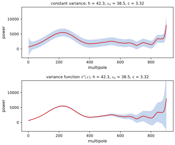
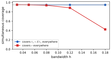
Remark 5.107 points to bootstrap bands (Härdle and Marron 1991; Hall 1993; Neumann and Polzehl 1998), which must resample in a way that reproduces the bias, for instance from an oversmoothed pilot fit.
5.8 Average Coverage
pp. 94–95 A weaker requirement than (5.12) is average coverage on \([0,1]\): \(C=\int_0^1\P(r(x)\in[\ell(x),u(x)])\,\d x\) (Wahba 1983; Nychka 1988; Cummins, Filloon and Nychka 2001). Suppose \(B_n(\alpha)=\{r:\|\hr-r\|\le s_n(\alpha)\}\) is a confidence ball, \(\P(r\in B_n(\alpha))\ge1-\alpha\), in the \(L_2[0,1]\) norm (Chapters 7 and 8 construct such balls).
Result 5.108 (bands with average coverage from a confidence ball; after Juditsky and Lambert-Lacroix 2003) p. 94, (5.108)
\[ \ell(x)=\hr(x)-s_n(\alpha/2)\sqrt{\frac2\alpha},\qquad u(x)=\hr(x)+s_n(\alpha/2)\sqrt{\frac2\alpha} \tag{5.108} \]has average coverage \(C\ge1-\alpha\).
Filling the gap 5.18: the steps of the proof pp. 94–95
Proof
Let \(U\sim\mathrm{Unif}(0,1)\) be independent of the data. By Fubini's theorem, \[ C=\int_0^1\P(r(x)\in[\ell(x),u(x)])\,\d x=\P(r(U)\in[\ell(U),u(U)]) \]. Write \(s=s_n(\alpha/2)\), \(t=s\sqrt{2/\alpha}\) and \(A=\{r\in B_n(\alpha/2)\}=\{\|\hr-r\|\le s\}\), so \(\P(A^c)\le\alpha/2\). Then
\[ 1-C=\P(|\hr(U)-r(U)|\gt t)\le\P(|\hr(U)-r(U)|\gt t,\ A)+\P(A^c). \]For the first term apply Markov's inequality to the non-negative variable \(I_A|\hr(U)-r(U)|^2\):
\[ \P(|\hr(U)-r(U)|\gt t,\ A)=\P\big(I_A|\hr(U)-r(U)|^2\gt t^2\big)\le\frac{\E\big[I_A|\hr(U)-r(U)|^2\big]}{t^2}. \]Condition on the data (on which \(A\) and \(\hr\) depend) and integrate over \(U\) first: \[ \E[I_A|\hr(U)-r(U)|^2\given\text{data}]=I_A\int_0^1|\hr(u)-r(u)|^2\,\d u=I_A\|\hr-r\|^2\le s^2 \]. Hence the first term is at most \(s^2/t^2=\alpha/2\), and \(1-C\le\alpha/2+\alpha/2=\alpha\). ∎
The constant \(\sqrt{2/\alpha}\) (4.5 for \(\alpha=0.1\)) comes from Markov's inequality and makes the band wide; the point of the construction is that it covers \(r\) itself, not \(\br\), because the ball does.
5.9 Summary of Linear Smoothing
Summary: estimate and band for a linear smoother p. 95, (5.109)
- Choose a smoother, i.e. the form of the weights \(\bl(x)\); local linear (Theorem 5.60) is a good default.
- Choose \(h\) by cross-validation (5.35), and plot the score.
- Estimate \(\sigma^2(x)\) (Section 5.6, with the correction of Filling the gap 5.14).
- Compute \(\kappa_0\) from (5.101) and \(c\) from (5.102).
- An approximate \(1-\alpha\) band for \(\br(x)=\E\hr(x)\) is
Example 5.110 (LIDAR): we find \(\kappa_0=16.7\) and \(c=3.07\), the band of Figure 5.4.
5.10 Local Likelihood and Exponential Families
pp. 96–99 For binary or count responses the model (5.1) with Gaussian errors is unnatural, although its asymptotics do not need normality. \(Y\) given \(x\) follows an exponential family if
\[ f(y\given x)=\exp\Big\{\frac{y\theta(x)-b(\theta(x))}{a(\phi)}+c(y,\phi)\Big\}, \tag{5.111} \]so that \(r(x)=\E(Y\given X=x)=b'(\theta(x))\) and \(\sigma^2(x)=a(\phi)b''(\theta(x))\). A generalised linear model assumes
\[ Y\given X=x\sim f(y\given x),\qquad g(\E(Y\given X=x))=x^\T\beta \tag{5.112} \]for a known link \(g\). For \(Y\sim\mathrm{Binomial}(m,r(x))\), \(\theta=\log\{r/(1-r)\}\), \(b(\theta)=m\log(1+e^\theta)\), \(a\equiv1\). (The mean and variance formulas follow by differentiating \(\int f(y\given x)\,\d y=1\) twice in \(\theta\): \(\E Y=b'(\theta)\), \(\V Y=a(\phi)b''(\theta)\).)
For \(Y_i\sim\mathrm{Bernoulli}(r(x_i))\) with \(\xi(x)=\log\{r(x)/(1-r(x))\}\), the log-likelihood is \(\sum_i\ell(Y_i,\xi(x_i))\) (5.113) with
\[ \ell(y,\xi)=\log\Big\{\Big(\frac{e^\xi}{1+e^\xi}\Big)^y\Big(\frac1{1+e^\xi}\Big)^{1-y}\Big\}=y\xi-\log(1+e^\xi). \tag{5.114} \]Approximating \(\xi(u)\approx a_0+a_1(u-x)\) near \(x\) (the book writes \(x-u\) once; the sign is immaterial), the local log-likelihood is
\[ \ell_x(a)=\sum_{i=1}^nK\Big(\frac{x-X_i}h\Big)\Big\{Y_i(a_0+a_1(X_i-x))-\log\big(1+e^{a_0+a_1(X_i-x)}\big)\Big\}, \]and with \(\hat a(x)\) its maximiser,
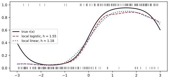
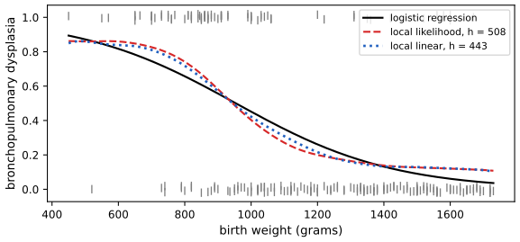
\[ \hr(x)=\frac{e^{\hat a_0(x)}}{1+e^{\hat a_0(x)}}. \tag{5.115} \]\(\ell_x\) is concave in \(a\) (it is a weighted logistic log-likelihood), so Newton–Raphson, i.e. the reweighted least squares of Section 5.1 with kernel weights, finds the maximiser when it exists (it fails to exist if the data in the window are separable). The bandwidth is chosen by the leave-one-out log-likelihood
\[ \mathrm{CV}=\sum_{i=1}^n\ell\big(Y_i,\hat\xi_{(-i)}(x_i)\big). \tag{5.116} \]There is no exact shortcut, but Loader (1999a) gives an approximation, with \(\dot\ell(y,\xi)=y-p(\xi)\), \(\ddot\ell(y,\xi)=-p(\xi)(1-p(\xi))\), \(p(\xi)=e^\xi/(1+e^\xi)\), \(\mathbf{V}_x\) diagonal with entries \(-\ddot\ell(Y_j,\hat a_0+\hat a_1(x_j-x))\), and
\[ m(x)=K(0)\,e_1^\T(\bX_x^\T\bW_x\mathbf{V}_x\bX_x)^{-1}e_1. \tag{5.118} \]Filling the gap 5.19: Loader's approximation to the cross-validated log-likelihood p. 98, (5.117)
Derivation
Fix \(x=x_i\) and write \(\hat a=\hat a(x_i)\), \(\mathbf{H}=\bX_x^\T\bW_x\mathbf{V}_x\bX_x\) (minus the Hessian of \(\ell_x\) at \(\hat a\)). Removing observation \(i\) removes from \(\ell_x\) the term \(K(0)\ell(Y_i,a_0)\) (at \(x=x_i\) its covariate row is \(e_1^\T\)). One Newton step from \(\hat a\) for the reduced criterion, whose gradient at \(\hat a\) is \(0-K(0)\dot\ell(Y_i,\hat a_0)e_1\), gives
\[ \hat a_{(-i)}\approx\hat a-K(0)\dot\ell(Y_i,\hat a_0)\mathbf{H}^{-1}e_1,\qquad \hat\xi_{(-i)}(x_i)\approx\hat\xi(x_i)-m(x_i)\,\dot\ell(Y_i,\hat\xi(x_i)). \]A first-order expansion of \(\ell(Y_i,\cdot)\) around \(\hat\xi(x_i)\) then gives
\[ \mathrm{CV}\approx\sum_{i=1}^n\ell\big(Y_i,\hat\xi(x_i)\big)-\sum_{i=1}^nm(x_i)\,\dot\ell\big(Y_i,\hat\xi(x_i)\big)^2. \]The book's (5.117) has \(\ell_x(\hat a)\) as the first term and a plus sign before the sum; the first term must be the fitted log-likelihood \(\sum_i\ell(Y_i,\hat\xi(x_i))\) and the correction must be subtracted (leaving out a point can only make its fit worse to first order: the penalty is a positive multiple of the squared score). For Gaussian \(\ell\) the same derivation reproduces Theorem 5.34 to first order. Numerically, for the simulated data of Figure 5.12 the approximation is within 2 percent of the exact leave-one-out score (5.116) for \(h\ge0.9\), but far too optimistic for small bandwidths (at \(h=0.4\): \(-113\) against the exact \(-148\)), where a window holds few points and one Newton step is a poor description of refitting; there it would select too small an \(h\), so the figure uses the exact refit. The effective degrees of freedom are \(\nu=\sum_im(x_i)\E(-\ddot\ell(Y_i,\hat a_0))\), the analogue of \(\tr\mathbf{L}\). ∎
See also (companion course): Statistical Learning, Section 6.5 (local likelihood) and its local logistic demo.
5.11 Scale-Space Smoothing
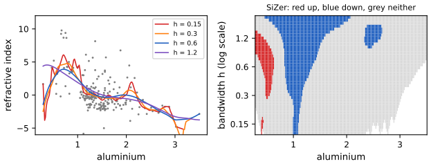
pp. 99–100 Chaudhuri and Marron (1999, 2000) avoid choosing a bandwidth: regard \(\hat r_h\) as an estimate of \(\bar r_h=\E\hat r_h\) and look at the whole scale-space surface \(\{\hat r_h(x):x\in\mathcal{X},h\in\mathcal{H}\}\). Their SiZer (significant zero crossings of derivatives) marks, for each \((x,h)\), whether \(\bar r_h'(x)\) is significantly positive, negative or neither, using \(\hat r_h'(x)\) and its standard error. Since \(\hat r_h'\) is a linear smoother (5.143), its standard error is \(\hs\|\bl(x,1)\|\), and simultaneous significance over \(x\) for each \(h\) follows from the tube formula applied to \(\bl(x,1)\) (Exercise 21). Because the target is \(\bar r_h\) and not \(r\), the bias problem of Section 5.7 disappears: each row of the map is an exact statement about the curve seen at resolution \(h\).
5.12 Multiple Regression
pp. 100–111 With \(x\in\R^d\),
\[ Y=r(x_1,\dots,x_d)+\epsilon. \tag{5.121} \]If \(r\) has square-integrable second derivatives, the optimal rate of the risk is \(n^{-4/5}\) in one dimension and \(n^{-4/(4+d)}\) in \(d\) dimensions.
Filling the gap 5.20: the sample size needed in \(d\) dimensions p. 101
Derivation
For a local linear estimator with a single bandwidth \(h\) in \(d\) dimensions, the bias is of order \(h^2\) (Theorem 5.125 with \(H=h^2\bI\)) and the variance of order \(1/(nh^d)\) (a window of volume \(h^d\) contains about \(nh^d\) points). Balancing \(h^4\asymp1/(nh^d)\) gives \(h\asymp n^{-1/(4+d)}\) and risk \(\asymp n^{-4/(4+d)}\); Stone (1982) proved that no estimator does better uniformly over such a smoothness class. To match the accuracy \(\delta=n^{-4/5}\) of a one-dimensional problem with \(n\) points, a \(d\)-dimensional one needs \(m^{-4/(4+d)}=n^{-4/5}\), i.e.
\[ m=n^{(4+d)/5}=n^{cd},\qquad c=\frac{4+d}{5d}, \]as the book says. For a fixed accuracy \(\delta\), \(m=\delta^{-(4+d)/4}=\delta^{-1}\cdot(\delta^{-1/4})^d\): the sample size grows exponentially in \(d\). With \(\delta=0.01\) (\(n=316\) in one dimension): \(d=2\) needs 3,162, \(d=5\) needs 316,228, \(d=10\) needs \(3\times10^{8}\). ∎
See also (companion course): Probability and Statistical Inference, Filling the gap 20.13 (Silverman's table for density estimation) and the curse of dimensionality demo.
Local regression. With a bandwidth matrix \(H\), \(K_H(x)=|H|^{-1/2}K(H^{-1/2}x)\); after scaling the covariates, \(h^{-d}K(\|x\|/h)\). The local linear criterion and estimate are
\[ \sum_{i=1}^nw_i(x)\Big(Y_i-a_0-\sum_{j=1}^da_j(x_{ij}-x_j)\Big)^2,\qquad w_i(x)=K(\|x_i-x\|/h), \tag{5.122} \] \[ \hr(x)=\hat a_0, \tag{5.123} \] \[ \hat a=(\bX_x^\T\bW_x\bX_x)^{-1}\bX_x^\T\bW_x\bY, \tag{5.124} \]where row \(i\) of \(\bX_x\) is \((1,x_{i1}-x_1,\dots,x_{id}-x_d)\).
Theorem 5.125 (Ruppert and Wand 1994) p. 102, (5.126)–(5.127)
Under regularity conditions, at an interior point \(x\), conditionally on the design, the multivariate local linear estimator has bias
\[ \tfrac12\mu_2(K)\,\tr(H\mathcal{H})+\oP(\tr H) \tag{5.126} \](\(\mathcal{H}\) the Hessian of \(r\) at \(x\), \(\int uu^\T K(u)\,\d u=\mu_2(K)\bI\)) and variance
\[ \frac{\sigma^2(x)\int K(u)^2\,\d u}{n|H|^{1/2}f(x)}\{1+\oP(1)\}. \tag{5.127} \]At the boundary the bias is still \(\OP(\tr H)\).
Filling the gap 5.21: why the one-dimensional argument carries over p. 102
Sketch
The weights reproduce affine functions exactly (\(\sum_i\ell_i=1\), \(\sum_i\ell_i(x_i-x)=0\)), as in Filling the gap 5.7, so the bias is \(\tfrac12\sum_i\ell_i(x_i-x)^\T\mathcal{H}(x_i-x)+o(\tr H)\). Substituting \(x_i=x+H^{1/2}u\), the weights are \(\ell_i\approx K_H(x_i-x)/(nf(x))\) to first order, so \[ \sum_i\ell_i(x_i-x)(x_i-x)^\T\approx\int K(u)H^{1/2}uu^\T H^{1/2}\d u=\mu_2(K)H \], and the bias is \(\tfrac12\mu_2\tr(\mathcal{H}H)\); the gradient of \(f\), which would give design bias, multiplies \(\sum_i\ell_i(x_i-x)=0\). The variance is \[ \sigma^2\sum_i\ell_i^2\approx\sigma^2\int K_H^2(v)f(x)\,\d v/(nf(x))^2\cdot n=\sigma^2R(K)/(n|H|^{1/2}f(x)) \]. At the boundary the moment matrix changes but affine reproduction still holds, so the bias remains of order \(\tr H\). ∎
Thin-plate splines. For \(d=2\), minimise \(\sum_i(Y_i-r(x_{i1},x_{i2}))^2+\lambda J(r)\) with \[ J(r)=\iint\{(\partial^2r/\partial x_1^2)^2+2(\partial^2r/\partial x_1\partial x_2)^2+(\partial^2r/\partial x_2^2)^2\}\,\d x_1\d x_2 \] (the book's display drops the squares on the last two terms); the minimiser is a thin-plate spline (Green and Silverman 1994).
Additive models.
\[ Y=\alpha+\sum_{j=1}^dr_j(x_j)+\epsilon, \tag{5.128} \]identified by \(\alpha=\overline Y\) and \(\sum_ir_j(x_{ij})=0\) for each \(j\).
The backfitting algorithm p. 103
Initialise \(\hat\alpha=\overline Y\) and \(\hat r_1,\dots,\hat r_d\) (e.g. 0). Iterate until convergence: for \(j=1,\dots,d\), compute the partial residuals \(\tilde Y_i=Y_i-\hat\alpha-\sum_{k\ne j}\hat r_k(x_{ik})\); smooth \(\tilde Y\) against \(x_j\) to get \(\hat r_j\); centre it, \(\hat r_j\leftarrow\hat r_j-n^{-1}\sum_i\hat r_j(x_{ij})\).
Filling the gap 5.22: what backfitting solves, and when it converges pp. 103–104
Derivation
With fixed linear smoothers \(\mathbf{S}_j\) (\(n\times n\)) and \(\mathbf{f}_j\) the vector of \(\hat r_j(x_{ij})\), a fixed point of backfitting solves the normal equations \(\mathbf{f}_j=\mathbf{S}_j\big(\bY-\hat\alpha\mathbf{1}-\sum_{k\ne j}\mathbf{f}_k\big)\), \(j=1,\dots,d\): a linear system of size \(nd\), and backfitting is its block Gauss–Seidel iteration. If every \(\mathbf{S}_j\) is symmetric with eigenvalues in \([0,1]\) (smoothing splines, regression splines), the fixed point minimises the penalised criterion \(\|\bY-\alpha-\sum_j\mathbf{f}_j\|^2+\sum_j\mathbf{f}_j^\T(\mathbf{S}_j^{-}-\bI)\mathbf{f}_j\), and backfitting converges to a solution (Buja, Hastie and Tibshirani 1989): Gauss–Seidel for a positive semidefinite quadratic. For non-symmetric smoothers such as local linear regression, convergence holds when the product of the "centred" smoothers is a contraction, which is the usual case but not guaranteed. In particular, a fixed point is a linear smoother of \(\bY\): \(\hat{\mathbf{f}}_j=\mathbf{L}_j\bY\), which is what makes bands possible (Exercise 23). Re-choosing the bandwidths by cross-validation inside the loop, as in Example 5.129, makes the map non-linear and voids this theory; in practice it settles quickly. ∎
See also (companion courses): Probability and Statistical Inference, Filling the gap 20.19; Statistical Learning, Section 9.1 and its backfitting demo.
Example 5.129 uses the rock data: 48 rock samples from a petroleum reservoir, response permeability, covariates the area of pores, the perimeter and the shape (perimeter\(/\sqrt{\text{area}}\)). The book's figures for this example were drawn with the columns shifted by one (Notes on the book); here the stated model, log permeability on area, perimeter and shape, is fitted.
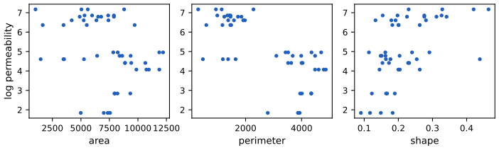
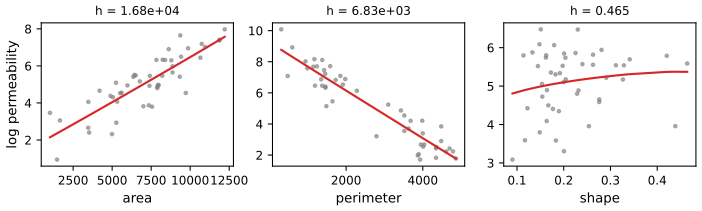
A three-dimensional local linear fit (5.123) on the standardised covariates, with \(h\) by cross-validation, gives \(h=2.4\) and \(\nu=12.6\) (the book, with its variables, reports \(h\approx3.2\)). Its residuals and those of the additive model are compared below.
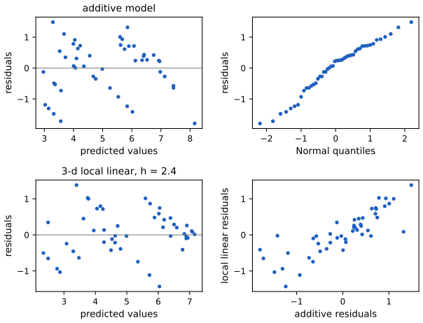
Projection pursuit regression (Friedman and Stuetzle 1981) approximates \(r\) by \(\mu+\sum_{m=1}^Mr_m(\alpha_m^\T x)\) with unit vectors \(\alpha_m\). With \(\mu=\overline Y\), centred \(Y\), standardised covariates and a one-dimensional smoother \(S\): (1) set \(\hat\epsilon_i=Y_i\), \(m=0\); (2) find the unit \(\alpha\) maximising \(I(\alpha)=1-\sum_i(\hat\epsilon_i-S(\alpha^\T x_i))^2/\sum_i\hat\epsilon_i^2\), set \(z_{mi}=\alpha^\T x_i\), \(\hat r_m(z_{mi})=S(z_{mi})\); (3) \(m\leftarrow m+1\), \(\hat\epsilon_i\leftarrow\hat\epsilon_i-\hat r_m(z_{mi})\); repeat until \(m=M\). The maximisation over the sphere is not convex; the code uses several starting directions and the Nelder–Mead method, with a local linear smoother whose span is chosen by GCV (the book used R's ppr with smoothing splines).
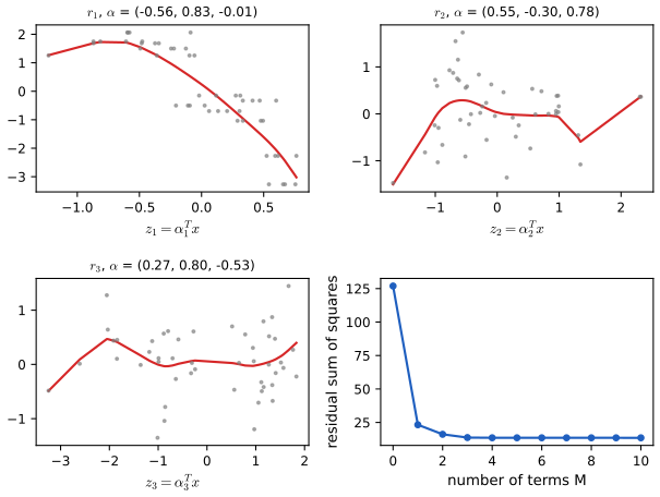
See also (companion course): Statistical Learning, Section 11.2 and its projection pursuit demo.
Regression trees. A tree is
\[ r(x)=\sum_{m=1}^Mc_mI(x\in R_m) \tag{5.131} \]for disjoint rectangles \(R_m\). The tree is grown by splitting a rectangle on a covariate \(j\) at a point \(s\) into \(\{x_j\le s\}\) and \(\{x_j\gt s\}\), with the leaf means as \(c_1,c_2\) and \((j,s)\) chosen to minimise the residual sum of squares, recursively. Figure 5.18 of the book is a schematic of such a tree and its rectangles (not reproduced: it contains no data). A large tree is then pruned by minimising, over subtrees \(T\) with leaves \(R_m\) of sizes \(N_m\), leaf means \(\hat c_m\) and \(Q_m(T)=N_m^{-1}\sum_{x_i\in R_m}(Y_i-\hat c_m)^2\),
\[ C_\alpha(T)=\sum_{m=1}^{|T|}N_mQ_m(T)+\alpha|T|, \tag{5.132} \]with \(\alpha\) chosen by cross-validation.
Filling the gap 5.23: the split search is exact, and the pruned trees are nested p. 108
Derivation
Splits. For fixed \((j,s)\) the best constants are the means (they minimise each sum of squares separately). As \(s\) moves between consecutive distinct values of \(x_j\) the partition does not change, so only \(n-1\) split points per covariate need checking; with the data sorted on \(x_j\) and running sums of \(Y\) and \(Y^2\), all of them cost \(O(n)\), so a split costs \(O(dn\log n)\).
Pruning. For each \(\alpha\) there is a unique smallest subtree \(T_\alpha\) minimising \(C_\alpha\), and \(T_\alpha\) shrinks as \(\alpha\) grows; the whole path is obtained by weakest-link pruning: repeatedly collapse the internal node \(t\) with the smallest \(g(t)=\{R(t)-R(T_t)\}/(|T_t|-1)\), where \(R(t)\) is the sum of squares if \(t\) is a leaf and \(T_t\) the branch below \(t\) (Breiman, Friedman, Olshen and Stone 1984, Chapter 10). Proof idea: \(C_\alpha\) is additive over branches, so a branch is worth keeping iff its decrease in sum of squares exceeds \(\alpha\) times the number of leaves it adds, i.e. iff \(g(t)\gt \alpha\); collapsing in order of \(g\) therefore produces the nested sequence of minimisers. So cross-validating \(\alpha\) means choosing among finitely many nested trees. ∎
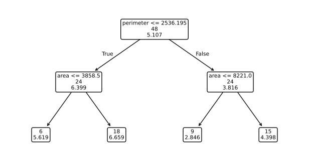
See also (companion course): Statistical Learning, Section 9.2.2 and its tree pruning demo.
MARS (Friedman 1991) uses the reflected pairs \(\ell(x,j,t)=(x_j-t)I(x_j\gt t)\) and \(r(x,j,t)=(t-x_j)I(x_j\lt t)\), knots \(t\) at the observed \(x_{ij}\), the collection \(\mathcal{C}=\bigcup_j\mathcal{C}_j\), and models
\[ r(x)=\beta_0+\sum_{m=1}^M\beta_mh_m(x), \tag{5.134} \]each \(h_m\) in \(\mathcal{C}\) or a product of such functions. A forward pass adds the pair (times an existing term) that most reduces the residual sum of squares; a backward pass deletes terms by GCV with an effective number of parameters \(M+c(M-1)/2\), \(c\approx3\) (Hastie, Tibshirani and Friedman 2001, Section 9.4; implemented in the code and used in Exercise 22). Tensor product models \(r(x)=\sum_m\beta_mh_m(x)\) (5.135) return in Chapter 8.
See also (companion course): Statistical Learning, Section 9.4 (MARS) and its MARS demo.
5.13 Other Issues
Plug-in bandwidths. pp. 111–112 For local linear regression with a random design (Fan and Gijbels 1996, Section 4.2), the asymptotically optimal bandwidth is
\[ h_*=\Big(\frac{C\int\sigma^2(x)/f(x)\,\d x}{n\int(r^{(2)}(x))^2\,\d x}\Big)^{1/5}, \tag{5.136} \] \[ C=\frac{\int K^2(t)\,\d t}{\big(\int t^2K(t)\,\d t\big)^2}. \tag{5.137} \](The book prints \(\int K(t)\,\d t\) in the denominator of (5.137), which is 1 for every kernel; the \(t^2\) is needed: Notes on the book.) The crude rule: fit a global quartic \(\tilde r\) by least squares, let \(\tilde\sigma^2\) be its mean squared residual, take \(f\) uniform on the range \((a,b)\) of the \(X_i\), and estimate \[ n\int r''^2\approx\sum_ir''(X_i)^2/f(X_i)=(b-a)\sum_i\tilde r^{(2)}(X_i)^2 \], so that
\[ \hat h_*=\Big(\frac{C\tilde\sigma^2(b-a)}{\sum_{i=1}^n(\tilde r^{(2)}(X_i))^2}\Big)^{1/5}. \tag{5.138} \]Filling the gap 5.24: (5.136) from Theorem 5.65, and the plug-in steps pp. 111–112
Derivation
By (5.66) and (5.68) the local linear estimator has pointwise MSE \(\tfrac14h^4\mu_2^2r''(x)^2+\sigma^2(x)R(K)/(nhf(x))\). Integrate against \(\d x\) (or against \(f\) for a prediction-weighted risk) and minimise \(\tfrac14Ah^4+B/(nh)\) with \(A=\mu_2^2\int r''^2\) and \(B=R(K)\int\sigma^2/f\) as in Filling the gap 5.6: \[ h_*^5=B/(nA)=\{R(K)/\mu_2^2\}\int(\sigma^2/f)/\{n\int r''^2\} \], which is (5.136) with \(C=R(K)/\mu_2^2\). In (5.138), \(\int\sigma^2/f=\tilde\sigma^2(b-a)^2\) for constant variance and uniform \(f\), and \[ \int r''^2=\int(r''^2/f)f\approx n^{-1}\sum_ir''(X_i)^2/f(X_i)=n^{-1}(b-a)\sum_ir''(X_i)^2 \] by the law of large numbers; substituting gives (5.138). For the tricube kernel \(C=34.15\). On the LIDAR data (5.138) gives \(\hat h_*=44.6\), against 37 from cross-validation: the quartic pilot is a reasonable but rough stand-in for \(r''\). ∎
Testing for linearity. To test \(H_0:r(x)=\beta_0+\beta_1x\), let \(\mathbf{H}\) be the hat matrix of the linear fit, \(\mathbf{L}\) that of the nonparametric fit, \(\lambda=\tr((\mathbf{L}-\mathbf{H})^\T(\mathbf{L}-\mathbf{H}))\) and
\[ T=\frac{\|\mathbf{L}\bY-\mathbf{H}\bY\|^2/\lambda}{\hs^2}, \]with \(\hs^2\) from (5.86). Loader (1999a): under \(H_0\), \(T\) is roughly \(F_{\lambda,\,n-2\nu_1+\nu_2}\) with \(\nu_1=\tr\mathbf{L}\), \(\nu_2=\tr(\mathbf{L}^\T\mathbf{L})\). (The book's display has no square on the norm and writes "\(\nu\)" for \(\lambda\).)
Filling the gap 5.25: why an \(F\) approximation p. 112
Derivation
Under \(H_0\), \(\mathbf{r}=\bX\beta\) with \(\bX=(\mathbf{1},x)\). \(\mathbf{H}\mathbf{r}=\mathbf{r}\), and a local linear smoother reproduces lines exactly (Filling the gap 5.7), so \(\mathbf{L}\mathbf{r}=\mathbf{r}\) too: \((\mathbf{L}-\mathbf{H})\bY=(\mathbf{L}-\mathbf{H})\epsilon\), with no bias at all. By (5.87), \(\E\|(\mathbf{L}-\mathbf{H})\bY\|^2=\sigma^2\lambda\), so the numerator has mean \(\sigma^2\); the denominator is consistent with mean exactly \(\sigma^2\) under \(H_0\) (Filling the gap 5.12, zero bias term). With Normal errors the numerator is a weighted sum of \(\chi^2_1\) variables with weights the eigenvalues of \((\mathbf{L}-\mathbf{H})^\T(\mathbf{L}-\mathbf{H})\); matching its mean to that of \(\chi^2_\lambda/\lambda\) gives the \(F\) form (a one-moment approximation; a two-moment Satterthwaite match would also adjust the degrees of freedom, and numerator and denominator are not exactly independent). On the LIDAR data (\(h=37\)) \(T=59.8\) on \(\lambda=5.8\) and 210.5 degrees of freedom: linearity is rejected overwhelmingly, as Figure 5.4 makes obvious. Härdle and Mammen (1993) calibrate the test by the bootstrap instead. ∎
Optimality. pp. 112–113 Let \(x_0\) be interior, the design random with density \(f\), \(f(x_0)\gt 0\) and \(\sigma(x)\) continuous at \(x_0\), and
\[ \mathcal{F}=\Big\{r:\ |r(x)-r(x_0)-(x-x_0)r'(x_0)|\le\frac C2(x-x_0)^2\Big\} \](the book prints \(C|x-x_0|\) on the right; the quadratic bound is the class of Fan (1993) and the only one consistent with (5.140)). The linear minimax risk is
\[ R_n^L=\inf_{\hat\theta\in\mathcal{L}}\sup_{r\in\mathcal{F}}\E\big((\hat\theta-r(x_0))^2\given X_1,\dots,X_n\big), \tag{5.139} \]over all linear estimators \(\mathcal{L}\), and Fan and Gijbels (1996) show
\[ R_n^L=\frac34\,15^{-1/5}\Big(\frac{\sqrt C\,\sigma^2(x_0)}{nf(x_0)}\Big)^{4/5}\{1+\oP(1)\}, \tag{5.140} \]attained by the local linear estimator with the Epanechnikov kernel and \(h_*=\big(15\sigma^2(x_0)/(f(x_0)C^2n)\big)^{1/5}\). Over all estimators, \(R_n\) of (5.141), the same estimator is within a factor \(0.894^2\) of minimax (5.142).
Filling the gap 5.26: the linear minimax risk (5.140) p. 113
Derivation (continuous approximation)
A linear estimator \(\hat\theta=\sum_iw_iY_i\) has bias \(\sum_iw_ir(x_i)-r(x_0)\). If it does not reproduce lines, its bias is unbounded over \(\mathcal{F}\) (add \(a+b(x-x_0)\) with large \(a,b\)), so take \(\sum w_i=1\), \(\sum w_i(x_i-x_0)=0\). Then the bias is \(\sum_iw_i\rho(x_i)\) with \(|\rho(x)|\le\tfrac C2(x-x_0)^2\), and its supremum over \(\mathcal{F}\) is \(\tfrac C2\sum_i|w_i|(x_i-x_0)^2\) (take \(\rho=\tfrac C2\sgn(w_i)(x-x_0)^2\) at the design points). The worst-case MSE is
\[ \Big(\frac C2\sum_i|w_i|(x_i-x_0)^2\Big)^2+\sigma^2\sum_iw_i^2. \]In the continuous approximation \(w_i=K((x_i-x_0)/h)/(nhf(x_0))\) with \(K\ge0\), \(\int K=1\): bias \(\tfrac C2h^2\mu_2(K)\), variance \(\sigma^2R(K)/(nhf)\). Minimising over kernels with \(\int K=1\) and fixed \(\mu_2\) leads to the Epanechnikov kernel \(K(u)=\tfrac34(1-u^2)_+\) (the same variational problem as in density estimation, solved by Lagrange multipliers: \(K\propto(1-u^2/a^2)_+\)). For it \(R(K)=3/5\), \(\mu_2=1/5\), and the MSE \(\tfrac{C^2h^4}{100}+\tfrac{3\sigma^2}{5nfh}\) is minimised at \(h^5=15\sigma^2/(nfC^2)\), the stated \(h_*\). Writing it as \(Bh^4+A/h\) with \(A=3\sigma^2/(5nf)\), \(B=C^2/100\), the minimum is \(\tfrac54\,4^{1/5}A^{4/5}B^{1/5}\), and
\[ \tfrac54\,4^{1/5}\big(\tfrac35\big)^{4/5}100^{-1/5}=0.43633=\tfrac34\,15^{-1/5}, \]while \[ A^{4/5}B^{1/5}\propto(\sigma^2/(nf))^{4/5}C^{2/5}=(\sqrt C\sigma^2/(nf))^{4/5} \]: this is (5.140). With the class \(|\rho(x)|\le C|x-x_0|\) printed in the book, the worst-case bias would be of order \(h\), the risk of order \(n^{-2/3}\), and (5.140) could not hold. That the continuous weights are optimal among all linear weights is the content of the theorem of Fan (1993). ∎
Derivative estimation. pp. 113–115 From (5.50), \(r^{(k)}(x)\approx a_k\), estimated by
\[ \hr^{(k)}(x)=\hat a_k=\sum_{i=1}^n\ell_i(x,k)Y_i,\qquad \bl(x,k)^\T=e_{k+1}^\T(\bX_x^\T\bW_x\bX_x)^{-1}\bX_x^\T\bW_x, \tag{5.143} \]which is not the \(k\)th derivative of \(\hr\). Take \(p-k\) odd, e.g. \(p=k+1\). With \(\mu_j=\int u^jK\), \(\nu_j=\int u^jK^2\), \(S_{rs}=\mu_{r+s-2}\), \(S^*_{rs}=\nu_{r+s-2}\), \(c_p=(\mu_{p+1},\dots,\mu_{2p+1})^\T\), \(\tilde c_p=(\mu_{p+2},\dots,\mu_{2p+2})^\T\):
Theorem 5.144 (Fan and Gijbels 1996) p. 114, (5.145)–(5.147)
Under the conditions of Theorem 5.65 with \(r^{(p+1)}\) continuous,
\[ \V(\hr^{(k)}(x))=e_{k+1}^\T S^{-1}S^*S^{-1}e_{k+1}\,\frac{k!^2\sigma^2(x)}{f(x)nh^{1+2k}}+\oP\Big(\frac1{nh^{1+2k}}\Big). \tag{5.145} \]If \(p-k\) is odd, the bias is
\[ e_{k+1}^\T S^{-1}c_p\,\frac{k!}{(p+1)!}\,r^{(p+1)}(x)\,h^{p+1-k}+\oP(h^{p+1-k}). \tag{5.146} \]If \(p-k\) is even (with \(f'\) and \(r^{(p+2)}\) continuous and \(nh^3\to\infty\)), it is
\[ e_{k+1}^\T S^{-1}\tilde c_p\,\frac{k!}{(p+2)!}\Big\{r^{(p+2)}(x)+(p+2)r^{(p+1)}(x)\frac{f'(x)}{f(x)}\Big\}h^{p+2-k}+\oP(h^{p+2-k}). \tag{5.147} \](The book writes \(E(\hr^{(k)}(x))-r(x)\) for the bias, meaning \(-r^{(k)}(x)\), and \(m^{(p+1)}\) for \(r^{(p+1)}\).)
Filling the gap 5.27: where \(S\), \(S^*\) and the rule "take \(p-k\) odd" come from pp. 114–115
Sketch
In the scaled variable \(u=(x_i-x)/h\), \(\hat a_k=k!h^{-k}\hat b_k\) where \(\hat b\) is the weighted least squares fit of \(Y\) on \((1,u,\dots,u^p)\). The moment matrix is \(\bX^\T\bW\bX\approx nhf(x)S\) and \(\bX^\T\bW^2\bX\approx nhf(x)S^*\), so \(\V\hat b\approx\sigma^2(nhf)^{-1}S^{-1}S^*S^{-1}\), giving (5.145) after multiplying by \((k!h^{-k})^2\). For the bias, the Taylor remainder \(r^{(p+1)}(x)(hu)^{p+1}/(p+1)!\) projects onto \(\hat b\) through \(S^{-1}\int u^{p+1}(1,u,\dots,u^p)^\T K=S^{-1}c_p\). When \(p-k\) is even, the \((k+1)\)th entry of \(S^{-1}c_p\) vanishes by symmetry (the entries of \(c_p\) with an odd total power are zero, and \(S^{-1}\) preserves the even/odd pattern), so the next term, including the design-density derivative \(f'\), takes over: hence (5.147) and the rule "take \(p-k\) odd". The optimal bandwidth (5.148) balances (5.145) and the square of (5.146): \(h\asymp n^{-1/(2p+3)}\), and the risk for \(r^{(k)}\) is of order \(n^{-2(p+1-k)/(2p+3)}\), slower for higher derivatives. ∎
Variable bandwidths, correlated data. A bandwidth \(h(x)\) adapted to local smoothness (Fan and Gijbels 1995; Ruppert 1997) helps only modestly unless \(n\) is large and the noise small; Chapter 9 returns to spatial adaptation with wavelets. With dependent errors, cross-validation breaks down (it chooses too small an \(h\) under positive correlation) and the methods must use the dependence structure (Chapter 10).
Robustness and quantile regression. Replace the squared error in (5.52) by
\[ \sum_{i=1}^nw_i(x)\,\rho\Big(\frac{Y_i-a_0-a_1(x_i-x)-\dots-\frac{a_p}{p!}(x_i-x)^p}{s}\Big) \tag{5.149} \]with \(s\) a scale estimate: Huber's
\[ \rho'(t)=\max\{-c,\min(c,t)\} \tag{5.150} \]or
\[ \rho(t)=|t|+(2\alpha-1)t, \tag{5.151} \]which gives local quantile regression: \(\hr(x)\) estimates the \(\alpha\) quantile \(\xi(x)\) of \(Y\) given \(x\). The book's "common choice \(c=4.685\)" is the tuning constant of Tukey's biweight; for Huber's function the usual choice, with 95 percent efficiency at the Normal, is \(c=1.345\) (Notes on the book).
Filling the gap 5.28: the check function gives quantiles p. 116
Proof
\(\rho(t)=|t|+(2\alpha-1)t\) equals \(2\alpha t\) for \(t\ge0\) and \(-2(1-\alpha)t\) for \(t\lt 0\): twice the usual check function. For a random variable \(Y\) with cdf \(F\), \(g(a)=\E\rho(Y-a)\) is convex with right derivative \[ -2\alpha\P(Y\gt a)+2(1-\alpha)\P(Y\le a)=2\{F(a)-\alpha\} \]. So \(g\) decreases while \(F(a)\lt \alpha\) and increases once \(F(a)\gt \alpha\): the minimisers are the \(\alpha\) quantiles. For \(\alpha=\tfrac12\), \(\rho(t)=|t|\) and the median. Locally weighted, the same argument applied to the conditional distribution in a shrinking window shows that \(\hat a_0(x)\) estimates \(\xi(x)\). The code fits (5.149) by iteratively reweighted least squares (weights \(\rho(t)/t^2\) for the check function, \(\min(1,c/|t|)\) for Huber); Figure 5.S13 applies it to the glass data (Exercise 18). ∎
Measurement error (\(W_i=x_i+\delta_i\) observed instead of \(x_i\)) makes the naive regression of \(Y\) on \(W\) inconsistent (Chapter 10). Dimension reduction and variable selection (principal components, projection pursuit, Zhang 1991) have few methods that are both practical and theoretically justified. Confidence sets: the tube method of Section 5.7 extends to additive models and to linear smoothers in several dimensions (Sun and Loader 1994), not to trees, MARS or projection pursuit.
Undersmoothing. pp. 117–118 Chen and Qin (2000, 2002) study local linear intervals \(\hr(x)\pm z_\alpha\sqrt{v(x/h)\hs^2(x)/(nh\hat f(x))}\), with boundary-adjusted constants \(v(x/h)\) built from the incomplete moments \(\alpha_j(x/h)=\int_{-1}^{x/h}u^jK(u)\,\d u\). With \(nh^5\to0\) the coverage error is
\[ \P(r(x)\in I(x))=1-\alpha+O\Big(nh^5+h^2+\frac1{nh}\Big) \tag{5.152} \]in the interior and
\[ \P(r(x)\in I(x))=1-\alpha+O\Big(nh^5+h+\frac1{nh}\Big) \tag{5.153} \]near the boundary: local linear regression removes the boundary bias of the estimate but not the boundary error of the interval. Their empirical likelihood interval \(\{\theta:\ell(\theta)\le c_\alpha\}\) (5.154), \(c_\alpha\) the upper \(\alpha\) quantile of \(\chi^2_1\), restores the interior rate everywhere,
\[ \P(r(x)\in I(x))=1-\alpha+O\Big(nh^5+h^2+\frac1{nh}\Big), \tag{5.155} \]and balancing \(nh^5\) against \(1/(nh)\) gives the coverage-optimal \(h\asymp n^{-1/3}\), much smaller than the MSE-optimal \(n^{-1/5}\): a precise statement of how much to undersmooth, with a constant that depends on \(r\). These are research results whose proofs (Edgeworth expansions of studentised local linear estimators) are beyond these notes; the qualitative content is Filling the gap 5.15.
5.14 Bibliographic Remarks
p. 119 Good entry points: Fan and Gijbels (1996), Härdle (1990), Loader (1999a), Hastie and Tibshirani (1990), Hastie, Tibshirani and Friedman (2001); for splines Wahba (1990) and Ruppert, Wand and Carroll (2003); for local likelihood Loader (1999a) and Fan and Gijbels (1996); for variable bandwidths Fan and Gijbels (1995).
5.15 Appendix
pp. 119–120 Derivation of the tube formula (5.100). Let \(W(x)=\sum_iZ_iT_i(x)=\langle Z,T(x)\rangle\) with \(\|T(x)\|=1\). Writing \(Z=\|Z\|U\), where \(U=Z/\|Z\|\) is uniform on the unit sphere \(\mathcal{S}\subset\R^n\) and independent of \(\|Z\|^2\sim\chi^2_n\) (density \(h\)),
\[ \P\Big(\sup_xW(x)\gt c\Big)=\int_{c^2}^\infty\P\Big(\sup_x\langle U,T(x)\rangle\gt \frac c{\sqrt y}\Big)h(y)\,\d y. \]Since \(\|U-T(x)\|^2=2(1-\langle U,T(x)\rangle)\), the event is \(\{U\in\mathrm{tube}(\rho,\mathcal{M})\}\) with \(\rho=\sqrt{2(1-c/\sqrt y)}\), \(\mathcal{M}=\{T(x):x\in\mathcal{X}\}\) a curve on the sphere, and \(\mathrm{tube}(\rho,\mathcal{M})=\{u:d(u,\mathcal{M})\le\rho\}\). So the probability is \(\mathrm{volume}(\mathrm{tube}(\rho,\mathcal{M}))/A_n\), \(A_n=2\pi^{n/2}/\Gamma(n/2)\), and Hotelling (1939) and Naiman (1990) give, for small \(\rho\),
\[ \frac{\mathrm{volume}(\mathrm{tube}(\rho,\mathcal{M}))}{A_n}=\frac{\kappa_0}{A_2}\,\P\big(B_{1,(n-2)/2}\ge w^2\big)+\frac{\ell_0}{2A_1}\,\P\big(B_{1/2,(n-1)/2}\ge w^2\big),\qquad w=\frac c{\sqrt y}, \]where \(B_{a,b}\) is a Beta variable, \(A_2=2\pi\), \(A_1=2\), and \(\ell_0\) the number of end points of the curve (2 for an interval).
Filling the gap 5.29: integrating the tube volume gives (5.100) p. 120
Derivation
Use the polar decomposition backwards: if \(B\sim\mathrm{Beta}(a,b)\) is the squared length of the projection of \(U\) onto a fixed \(2a\)-dimensional subspace, then \(\|Z\|^2B\) is the squared length of the projection of \(Z\) itself, \(\sum_{j\le2a}Z_j^2\sim\chi^2_{2a}\). Hence, integrating over \(y=\|Z\|^2\),
\[ \int\P\big(B_{1,(n-2)/2}\ge c^2/y\big)h(y)\,\d y=\P(\chi^2_2\ge c^2)=e^{-c^2/2},\qquad \int\P\big(B_{1/2,(n-1)/2}\ge c^2/y\big)h(y)\,\d y=\P(\chi^2_1\ge c^2)=2(1-\Phi(c)). \]With the coefficients \(\kappa_0/A_2=\kappa_0/(2\pi)\) and \(\ell_0/(2A_1)=\ell_0/4\), and \(\ell_0=2\),
\[ \P\Big(\sup_xW(x)\gt c\Big)\approx\frac{\kappa_0}{2\pi}e^{-c^2/2}+\frac12\cdot2(1-\Phi(c))=\frac{\kappa_0}{2\pi}e^{-c^2/2}+1-\Phi(c), \]the one-sided formula. Applying it to \(W\) and \(-W\) (a curve and its antipodal image, together a tube of twice the volume when they do not overlap, which holds for large \(c\)) gives the two-sided (5.100). The terms neglected (the overlap of the two tubes, and the error of the volume formula, which is exact only for tubes thinner than the curve's critical radius) are of smaller order than \(e^{-c^2/2}\) as \(c\to\infty\). The same leading terms come from Rice's formula (Filling the gap 5.16): the curve length \(\kappa_0\) is the expected number of crossings per unit \(2\pi\), and the end points contribute the boundary terms \(1-\Phi(c)\). ∎
Rice's (1939, 1944) upcrossing formula, the book's second route, is
\[ \E(N_c)=\int_0^1\int_0^\infty y\,p_t(c,y)\,\d y\,\d t, \tag{5.156} \]with \(p_t\) the density of \((W(t),W'(t))\); it is carried out in Filling the gap 5.16.
Notes on the book
The book's website has no errata list. Each point below gives the evidence: a derivation in these notes or a computation with the book's own data.
Page 71: the relative rate of the bandwidth
\((\hat h-\hat h_0)/\hat h_0=\OP(n^{3/10}/n^{1/5})\) should read \(\OP(n^{-3/10}/n^{-1/5})=\OP(n^{-1/10})\), and likewise for \((\hat h_0-h_0)/h_0\); as printed the ratio grows with \(n\). See Filling the gap 5.5.
Page 73, (5.45) and (5.47): \(o((nh)^{-1})\), and \(\int x^2K\) instead of \(\int x^2K^2\)
The remainder in (5.45) is \(o((nh_n)^{-1})\), not \(o(nh_n^{-1})\). In (5.47) the denominator must contain \((\int x^2K(x)\,\d x)^2\), the square of the kernel's second moment that appears in the bias term of (5.45); \((\int x^2K^2)^2\) has the wrong dimension (it scales differently when \(K\) is rescaled). Derivation in Filling the gap 5.6.
Page 84: Silverman's equivalent kernel needs a factor \(1/n\)
The weights are \[ \ell_i(x)\approx K((x_i-x)/h(x_i))/(nf(x_i)h(x_i)) \]; without the \(1/n\) they would sum to about \(n\) instead of 1. Derivation in Filling the gap 5.11; Figure 5.S2 compares the corrected formula with the exact smoothing-spline weights (they agree in the interior).
Page 85, (5.86): \(\hr(x_i)\) in the numerator
The numerator of (5.86) is \(\sum_i(Y_i-\hr(x_i))^2\), the residual sum of squares, as the proof on page 86 uses (\(\bY-\hat{\mathbf{r}}=(\bI-\mathbf{L})\bY\)); the printed \(r(x_i)\) is a misprint.
Page 87, Example 5.92: the reported values are standard deviations
The book reports "\(\hs^2=408.29\)" from (5.86) and "\(\hs^2=394.55\)" from (5.89) for the first 400 CMB points. With the book's data (wmap.dat on its website) and the local linear fit at the cross-validated \(h=42.3\), (5.86) gives \(\hs^2=168{,}374\) and (5.89) gives \(155{,}670\), whose square roots are 410.3 and 394.55: Rice's value agrees to all printed digits. The reported numbers are \(\hs\), not \(\hs^2\) (the power varies between 0 and 6500, so a variance of 400 would be implausibly small anyway).
Pages 87–88, (5.95): the log-residual estimate of \(\sigma^2(x)\) is biased by a factor 0.28
Regressing \(Z_i=\log(\text{residual}_i^2)\) on \(x_i\) estimates \(\log\sigma^2(x)+\E\log\epsilon^2=\log\sigma^2(x)-1.2704\) for Normal errors, so \(e^{\hat q(x)}\) estimates \(0.28\,\sigma^2(x)\). The CMB data, for which the WMAP team's \(\sigma^2(x)\) is known, confirm it (Figure 5.9): on the log scale the corrected estimate is on average 0.28 above the known curve (a factor 1.3 in variance), the uncorrected one 0.99 below it (a factor 0.37). Proof and fix in Filling the gap 5.14.
Pages 77 and 95, Examples 5.59 and 5.110: \(\kappa_0\approx30\) for the LIDAR band
The book's fit (local linear, tricube, \(h=37\), 9 degrees of freedom) is reproduced exactly, yet its tube constant is \(\kappa_0=16.7\) (\(c=3.07\)), not 30 (\(c\approx3.25\)). Three independent checks agree with 16.7 rather than 30: the value is stable to 0.05 percent under grid refinement; the approximation of Exercise 20 gives \[ (b-a)\|K'\|/(h\|K\|)=330\times1.78/37=15.9 \]; and the same code gives \(\kappa_0=38.5\), \(c=3.32\) for the CMB band of Example 5.105, where the book reports 38.85 and 3.33. A value of 30 would correspond to \(h\approx20\). Also, for the LIDAR variance function the cross-validation score keeps decreasing as \(h\) grows (we stop at \(h=1500\)), whereas the book reports \(h=146\); the log variance is close to linear in the range, so the two give similar bands.
Page 98, (5.117): the first term and the sign of Loader's approximation
The approximation to the leave-one-out log-likelihood is \(\sum_i\ell(Y_i,\hat\xi(x_i))-\sum_im(x_i)\dot\ell(Y_i,\hat\xi(x_i))^2\): the first term is the fitted log-likelihood (not the local likelihood \(\ell_x(\hat a)\) at one point) and the correction is subtracted. Derivation in Filling the gap 5.19; with the plus sign the "cross-validated" score would exceed the fitted log-likelihood, which leaving points out cannot do to first order. The index of \(\mathbf{V}_x\) ("\(x_j-x_i\)") should be \(x_j-x\).
Page 102: the thin-plate penalty
The penalty is \[ \iint\{(\partial^2r/\partial x_1^2)^2+2(\partial^2r/\partial x_1\partial x_2)^2+(\partial^2r/\partial x_2^2)^2\} \], with every second derivative squared; as printed only the first term is squared, and the penalty would not be non-negative.
Pages 103–110, Example 5.129, Figures 5.14–5.16 and 5.19: the rock data columns are shifted
In rock.dat on the book's website the columns are area (1016 to 12212), peri (309 to 4864), shape (0.09 to 0.46) and perm (6.3 to 1300). The book's panels labelled "area" span about 1000 to 5000 (the range of peri), those labelled "perimeter" 0.1 to 0.4 (the range of shape), those labelled "shape" 0 to 1200 (the range of perm), and the response labelled "log permeability" spans 7 to 9 (the range of \(\log\) area, 6.9 to 9.4; \(\log\) perm runs from 1.8 to 7.2). The tree of Figure 5.19 is consistent with the same shift: splits at "area < 1403" and "peri < .1991" are values of peri and shape, and the leaf means 7.7 to 9.0 are values of \(\log\) area. So the book regressed \(\log(\text{area})\) on (peri, shape, perm). These notes fit the model the text states, \(\log(\text{perm})\) on (area, peri, shape); consequently the numbers differ from the book's.
Page 111, (5.137): \(C=\int K^2/(\int t^2K)^2\)
As printed, \(C=\int K^2(t)\,\d t/(\int K(t)\,\d t)^2=\int K^2\) for every kernel; the plug-in rule needs the second moment, \(C=R(K)/\mu_2(K)^2\), from minimising the asymptotic risk of Theorem 5.65 (Filling the gap 5.24).
Page 112: the linearity test statistic
The statistic is \(T=(\|\mathbf{L}\bY-\mathbf{H}\bY\|^2/\lambda)/\hs^2\), with the norm squared (otherwise its numerator has mean of order \(\sigma\sqrt\lambda\) and no \(F\) approximation applies), and the numerator degrees of freedom are \(\lambda\) (written \(\nu\)). See Filling the gap 5.25.
Page 113: the class \(\mathcal{F}\) for the minimax result
The class must bound the remainder of the linear Taylor approximation quadratically, \[ |r(x)-r(x_0)-(x-x_0)r'(x_0)|\le\tfrac C2(x-x_0)^2 \] (Fan 1993; Fan and Gijbels 1996, Section 3.4). With the printed bound \(C|x-x_0|\) the worst-case bias is of order \(h\) and the minimax rate is \(n^{-2/3}\), contradicting (5.140); with the quadratic bound the computation of Filling the gap 5.26 reproduces the constant \(\tfrac34\,15^{-1/5}\) and the bandwidth \(h_*\) exactly.
Page 116: Huber's tuning constant
\(c=4.685\) is the usual constant of Tukey's biweight (95 percent efficiency at the Normal). For Huber's \(\rho'(t)=\max\{-c,\min(c,t)\}\) the corresponding value is \(c=1.345\); with \(c=4.685\) Huber's estimator is almost least squares. Also, as \(c\to0\) Huber's \(\rho/c\) tends to the absolute error, as the book says, only after rescaling by \(c\).
Pages 120–121: Exercises 2 and 6 are the same
Both ask for a proof of Theorem 5.34. Exercise 6 is solved by reference to Exercise 2 below.
The data
The CMB data of the examples are the 899 WMAP power-spectrum points of wmap.dat on the book's website (multipoles 2 to 900), which match the book's description and reproduce its numbers (the \(h=42\) and \(h=160\) of Example 5.96, the \(\kappa_0\) and \(c\) of Example 5.105, the Rice estimate of Example 5.92 and 8.6 against 8.8 degrees of freedom in Example 5.84). The LIDAR fit (\(h=37\), 9 degrees of freedom) matches exactly. Simulated examples (Figures 5.6, 5.10, 5.12) use their own seeds and differ in detail. The air quality data of Exercises 14 and 22 are not on the website; R's airquality data set (New York, May to September 1973; 111 complete cases) is used.
5.16 Exercises
All 24 exercises of Chapter 5 (pp. 120–123), restated in my own words, with complete solutions (hidden). Computational solutions use the chapter's code.
Exercise 5.1. Write down the smoothing matrix of the regressogram of Example 5.24 and show that \(\nu=m\).
Solution
Ordering the data by bin, \(\mathbf{L}\) is block diagonal with blocks \(k_j^{-1}\mathbf{1}_{k_j}\mathbf{1}_{k_j}^\T\), each of trace 1, so \(\nu=m\) (the number of non-empty bins). Details and the \(9\times9\) example in Filling the gap 5.3.
Exercise 5.2. Prove Theorem 5.34.
Solution
See the proof under Theorem 5.34: with renormalised weights, \(\hat r_{(-i)}(x_i)=(\hr(x_i)-L_{ii}Y_i)/(1-L_{ii})\), hence \(Y_i-\hat r_{(-i)}(x_i)=(Y_i-\hr(x_i))/(1-L_{ii})\). For smoothing splines the identity holds for the genuine refit (Filling the gap 5.10); for local polynomials, refitting without \(i\) gives exactly the renormalised weights (Exercise 19).
Exercise 5.3. For the glass fragments data (refractive index \(Y\) against aluminium content \(x\)), fit \(Y=r(x)+\epsilon\) by (i) a regressogram, (ii) a kernel estimator, (iii) local linear regression and (iv) a smoothing spline, each tuned by cross-validation; estimate the variance; give 95 percent bands; and plot the effective kernels at a few values of \(x\).
Solution
Method: tricube kernel; the regressogram's number of bins, the bandwidths and \(\lambda\) chosen by (5.35); \(\hs\) from (5.86); bands \(\hr\pm c\hs\|\bl(x)\|\) with \(c\) from the tube formula (5.102), except for the regressogram, whose band is a set of \(m\) independent intervals, so the exact simultaneous constant is \(c=\Phi^{-1}\big((1+0.95^{1/m})/2\big)\) (the tube formula does not apply to a discontinuous \(T(x)\)). Results (214 fragments):
smoother tuning \(\nu\) CV score \(\hs\) \(\kappa_0\) \(c\) regressogram m = 4 4.0 7.11 2.63 n/a 2.49 kernel h = 0.478 6.1 6.94 2.59 11.9 2.96 local linear h = 0.528 7.4 7.00 2.56 12.0 2.97 smoothing spline by \(\nu\) 8.6 6.91 2.54 12.5 2.98 All four find a rise to about 4 near \(x=0.7\), a fall to about 0 by \(x=1.2\), a plateau, and a decline beyond 2; the bands are wide where the data are sparse (\(x\lt 0.8\) and \(x\gt 2.2\)). The effective kernels (Figure 5.S5): the regressogram's is a flat block that does not move with \(x\) inside a bin; the kernel estimator's is a tricube bump, lopsided where the data are uneven; the local linear one is similar in the interior but takes negative values near the edge of the data; the spline's is smooth with small negative side lobes, close to the local linear one.
Exercise 5.4. For the motorcycle data (time after impact, head acceleration), fit a curve by local linear regression with cross-validation.
Solution
Cross-validation over \(h\in[0.8,10]\) ms gives \(h=4.83\) ms (\(\nu=11.7\)). The fit is flat near 0 up to about 14 ms, drops to about \(-110\,g\) at 21 ms, rises to about \(+30\,g\) at 30 ms and settles (Figure 5.S7). The noise is strongly heteroscedastic (tiny before 14 ms), so a band should use a variance function (Section 5.6).
Exercise 5.5. Show that, for suitably smooth \(r\), Rice's estimator (5.89) is consistent.
Solution
See Filling the gap 5.13: for Lipschitz \(r\) the bias is at most \[ M^2(b-a)\max_i(x_{i+1}-x_i)/(2(n-1))\to0 \] and, with \(\E\epsilon^4\lt \infty\), the variance is \(O(1/n)\) because the squared differences are 1-dependent; Chebyshev's inequality concludes.
Exercise 5.6. Prove Theorem 5.34 (the same as Exercise 2).
Solution
See Exercise 2.
Exercise 5.7. Prove Theorem 5.60.
Solution
See the proof under Theorem 5.60: invert the \(2\times2\) matrix \(\bX_x^\T\bW_x\bX_x\) and take its first row times \(\bX_x^\T\bW_x\).
Exercise 5.8. Find conditions under which (5.86) is consistent.
Solution
Sufficient: \(\E\epsilon^4\lt \infty\); \(\nu=o(n)\), \(\tilde\nu=o(n)\); \(\|\mathbf{L}\|_{\rm op}\) bounded; and \(n^{-1}\|(\bI-\mathbf{L})\mathbf{r}\|^2\to0\) (the smoother is consistent at the design points). For a local linear smoother with a bounded kernel this holds when \(h\to0\), \(nh\to\infty\) and \(r\) is continuous. Proof in Filling the gap 5.12.
Exercise 5.9. For the glass data, examine the fit as a function of \(h\) by plotting fits with bands for many bandwidths; optionally apply SiZer.
Solution
Figure 5.S12 shows local linear fits for \(h=0.15,0.3,0.6,1.2\) and a SiZer map over 40 bandwidths from 0.12 to 2. The main features, a rise below aluminium 0.7 and a fall between 0.8 and 1.3, are significant over a wide range of scales; the bumps of the \(h=0.15\) fit beyond 1.5 are not, except a decrease near 2.5 at the largest scales. The band demo shows the bands as \(h\) moves.
Exercise 5.10. With five equally spaced knots on \((0,1)\), construct and plot the B-spline basis of order \(M\) for \(M=1,\dots,5\).
Solution
Figure 5.S6, by the recursion of Section 5.5 with \(M\) copies of each boundary knot: order \(M\) gives \(5+M\) functions, piecewise of degree \(M-1\): indicators (\(M=1\)), hats (\(M=2\)), quadratic, cubic and quartic bumps; each sums to 1 on \([0,1]\). Interactive version: spline demo, preset 2.
Exercise 5.11. For the motorcycle data, fit a cubic regression spline with equally spaced knots, choosing the number of knots by leave-one-out cross-validation; then fit a smoothing spline and compare.
Solution
The regression spline is a projection, so (5.35) is exact. The score is minimised at 9 interior knots (13 parameters); the smoothing spline with \(\lambda\) by cross-validation has \(\nu=12.5\) (Figure 5.S7). The three fits are close and follow the dip and the rebound; the regression spline shows small spurious oscillations in the flat part before 14 ms, because its equally spaced knots cannot be both dense enough for the sharp drop and sparse enough for the flat start. The CV curve over the number of knots is ragged (minimum 9, nearly as low at 5, 7 and 15), which is typical: knot placement, not only number, matters.
Exercise 5.12. Simulate 1000 observations of the Doppler function with \(x_i=i/n\) and \(\sigma=0.1,1,3\); fit local linear regression with cross-validation, plot the score, the fit and a 95 percent band.
Solution
Figure 5.S8 (middle column). Cross-validation gives about 157, 20 and 4 degrees of freedom for \(\sigma=0.1,1,3\). With \(\sigma=0.1\) the fit follows the oscillations down to \(x\approx0.05\); with \(\sigma=1\) only the slow oscillations beyond 0.25 survive; with \(\sigma=3\) the fit is almost a line. In every case the band contains \(\br\) (by construction) but not the Doppler function itself near 0: the bias problem at its most extreme. Use the local polynomial demo to see the CV curve.
Exercise 5.13. Repeat Exercise 12 with smoothing splines.
Solution
Figure 5.S8 (right column): about 181, 21 and 5 degrees of freedom. The spline fits are very close to the local linear ones, with slightly more degrees of freedom at \(\sigma=0.1\). On an equispaced design the spline's equivalent bandwidth is constant (Filling the gap 5.11), so, like local linear regression with one \(h\), it cannot adapt to the varying smoothness of the Doppler function. That is the motivation for the wavelet methods of Chapter 9.
Exercise 5.14. With the air quality data, model ozone as a function of temperature by kernel regression; compare bandwidths chosen by cross-validation, GCV, \(C_p\) and the plug-in rule.
Solution
Nadaraya–Watson with the tricube kernel, 111 complete days (Figure 5.S9): cross-validation \(h=3.17\)°F, GCV \(h=8.59\), \(C_p\) (with \(\hs^2\) from (5.86) at the CV fit) \(h=8.29\), plug-in (5.138) \(h=6.90\). The CV score has a shallow minimum at small \(h\) that GCV and \(C_p\) do not share: the temperatures are integers with many ties, so leaving out one point barely changes the fit at that point, and the leave-one-out score favours small bandwidths. GCV replaces the individual \(L_{ii}\) by their average and is less sensitive to ties. All four fits agree on the shape: flat around 20 ppb below 75°F, then rising steeply to about 90 ppb at 92°F.
Exercise 5.15. With \(Y_i\sim N(\mu_i,1)\) independent, find the minimisers of (a) \(\sum(Y_i-\mu_i)^2+\lambda\sum\mu_i^2\), (b) \(\sum(Y_i-\mu_i)^2+\lambda\sum|\mu_i|\), (c) \(\sum(Y_i-\mu_i)^2+\lambda\sum I(\mu_i\ne0)\).
Solution
Each criterion separates over \(i\). (a) \((Y-\mu)^2+\lambda\mu^2\) is minimised at \(\hat\mu_i=Y_i/(1+\lambda)\): linear shrinkage (ridge). (b) For \(\mu\ne0\) the derivative is \(-2(Y-\mu)+\lambda\sgn\mu\); the subgradient condition \(0\in-2(Y-\mu)+\lambda[-1,1]\) at \(\mu=0\) holds iff \(|Y|\le\lambda/2\). So \(\hat\mu_i=\sgn(Y_i)(|Y_i|-\lambda/2)_+\): soft thresholding at \(\lambda/2\) (the lasso). (c) The value is \(\lambda\) plus 0 if \(\mu=Y\), and \(Y^2\) if \(\mu=0\); so \(\hat\mu_i=Y_iI(Y_i^2\gt \lambda)\): hard thresholding at \(\sqrt\lambda\) (best subset). The three penalties reappear as the shrinkage rules of the normal means model (Chapter 7) and wavelet thresholding (Chapter 9).
Exercise 5.16. Show that a local polynomial smoother of order \(p\) reproduces polynomials of degree \(p\).
Solution
If \(Y_i=q(x_i)\) for a polynomial \(q\) of degree at most \(p\), Taylor's formula at \(x\) is exact: \[ q(u)=\sum_{j=0}^pq^{(j)}(x)(u-x)^j/j!=P_x(u;a^*) \] with \(a^*_j=q^{(j)}(x)\). Then the criterion (5.52) is 0 at \(a=a^*\), its minimum; when \(\bX_x^\T\bW_x\bX_x\) is invertible the minimiser is unique, so \(\hat a=a^*\) and \(\hr(x)=\hat a_0=q(x)\). Equivalently \(\sum_i\ell_i(x)(x_i-x)^j=\delta_{j0}\) for \(j\le p\): since \[ \bl(x)^\T\bX_x=e_1^\T(\bX_x^\T\bW_x\bX_x)^{-1}\bX_x^\T\bW_x\bX_x=e_1^\T \]. The derivative weights likewise satisfy \(\bl(x,k)^\T\bX_x=e_{k+1}^\T\).
Exercise 5.17. If \(r\) is \(L\)-Lipschitz on \([0,1]\), what is the maximum bias of a kernel estimator with bandwidth \(h\)?
Solution
For Nadaraya–Watson with a kernel supported on \([-1,1]\), the weights are non-negative and sum to 1, so \[ |\E\hr(x)-r(x)|=|\sum_i\ell_i(x)(r(x_i)-r(x))|\le\sum_i\ell_i(x)L|x_i-x|\le Lh \], because only \(|x_i-x|\le h\) carry weight. The bound is attained: take \(r(u)=L|u-x|\), which is in the class, at a point \(x\) where all weight sits at distance close to \(h\) (or with the more precise value \(L\sum_i\ell_i(x)|x_i-x|\approx Lh\int|u|K(u)\,\d u\) for a dense design). So \[ \sup_{r\in\mathcal{F}_{\rm lip}(L)}|\text{bias}|=L\sum_i\ell_i(x)|x_i-x|\le Lh \]: of order \(h\), not \(h^2\), because a Lipschitz function need not be differentiable, and the symmetry of the kernel cannot cancel a kink. With a kernel of unbounded support (Gaussian) the bound is \(Lh\int|u|K(u)\,\d u\) for a dense design.
Exercise 5.18. Fit a local quantile regression with \(\alpha=1/2\) to the glass data.
Solution
Local linear median regression, i.e. (5.149) with \(\rho(t)=|t|\), the bandwidth \(h=0.53\) of the local linear mean fit, by iteratively reweighted least squares (Figure 5.S13). The median curve agrees with the mean curve below aluminium 1.1 and above 2.3; between 1.2 and 2.2 it lies about 0.5 to 1 below the mean, because there the refractive indices are skewed upwards (a few large values pull the mean up). Near 3.1, where only a handful of points remain, the median fit is unstable. A Huber fit (\(c=1.345\)) lies in between.
Exercise 5.19. Show that the local polynomial weights have the form \(\ell_i(x)=K((x_i-x)/h)P_i(x)\) (5.158) for a polynomial \[ P_i(x)=\alpha_0+\alpha_1(x_i-x)+\dots+\alpha_p(x_i-x)^p \], and that omitting observation \(i\) gives the weights (5.32).
Solution
From (5.58), \[ \ell_i(x)=e_1^\T M^{-1}\bX_x^\T\bW_xe_i=K_i\,c^\T(1,(x_i-x),\dots,(x_i-x)^p/p!)^\T \] with \(c=M^{-1}e_1\) and \(M=\bX_x^\T\bW_x\bX_x\); so \(P_i(x)\) is a polynomial in \(x_i-x\) whose coefficients \(\alpha_j=c_j/j!\) do not depend on \(i\). (5.158) holds.
The second claim, that the genuine leave-one-out weights equal the renormalised ones, holds for the evaluation at the left-out point: we need \(\hat r_{(-i)}(x_i)=\sum_{j\ne i}\ell_j(x_i)Y_j/(1-\ell_i(x_i))\). Let \(M_{(-i)}=M-K_iz_iz_i^\T\) with \(z_i=(1,0,\dots,0)^\T\) the row of \(\bX_x\) for \(x_i\) when \(x=x_i\). By Sherman–Morrison, \[ M_{(-i)}^{-1}e_1=M^{-1}e_1+\frac{K_iM^{-1}e_1e_1^\T M^{-1}e_1}{1-K_ie_1^\T M^{-1}e_1}=\frac{M^{-1}e_1}{1-L_{ii}} \], since \(L_{ii}=\ell_i(x_i)=K_ie_1^\T M^{-1}e_1\) (here \(K_i=K(0)\)). Hence the leave-one-out weights at \(x_i\) are \(\ell_j(x_i)/(1-L_{ii})\) for \(j\ne i\), i.e. (5.32), because \(\sum_{k\ne i}\ell_k(x_i)=1-L_{ii}\). (At points \(x\ne x_i\) the refit weights are not a renormalisation, but (5.30) only uses \(x=x_i\).)
Exercise 5.20. If \(\ell_i(x)=K((x-x_i)/h)\) for a smooth kernel and equispaced \(x_i\), show that, ignoring boundary effects, \(\kappa_0\approx\frac{b-a}{h}\frac{\|K'\|}{\|K\|}\).
Solution
See the last paragraph of Filling the gap 5.16: \(\|T'(x)\|\approx h^{-1}\|K'\|/\|K\|\) because the cross term \(\sum_iK_iK_i'\approx\int KK'=0\); integrate over \([a,b]\). Here \(\|g\|^2=\int g^2\) over the real line (the book's \(\int_a^b\) is the same thing for a kernel supported inside the interval). For the tricube kernel \(\|K'\|/\|K\|=1.78\).
Exercise 5.21. Construct a confidence band for the derivative estimator \(\hr^{(k)}\) of (5.143).
Solution
\(\hr^{(k)}(x)=\bl(x,k)^\T\bY\) is a linear smoother with mean \(\bar r^{(k)}(x)=\bl(x,k)^\T\mathbf{r}\) and variance \(\sigma^2\|\bl(x,k)\|^2\). Put \(T(x)=\bl(x,k)/\|\bl(x,k)\|\), \(\kappa_0=\int\|T'\|\), \(c\) from (5.102), and the band \(\hr^{(k)}(x)\pm c\hs\|\bl(x,k)\|\) (or with \(\hs(x_i)\) inside the norm, as in (5.103)), with \(\hs\) from the regression fit, e.g. (5.86) at the cross-validated local linear fit. It covers \(\bar r^{(k)}\), with simultaneous probability about \(1-\alpha\), for the same reasons as in Section 5.7. Its width is of order \(\sigma(nh^{1+2k})^{-1/2}\) by (5.145). This is exactly what SiZer (Figure 5.S12) uses with \(k=1\), \(p=2\).
Exercise 5.22. With the air quality data, model ozone on solar radiation, wind and temperature by (i) multiple local linear regression, (ii) projection pursuit, (iii) an additive model, (iv) a regression tree and (v) MARS; compare.
Solution
Covariates standardised; each method's own tuning (bandwidth by leave-one-out CV for (i), \(h=2.10\); \(M=2\) terms for (ii); fixed bandwidth 1.5 per standardised covariate for (iii); cost-complexity pruning by CV for (iv); degree-2 MARS pruned by GCV for (v)); compared by the same 10-fold cross-validated mean squared prediction error (ppb\(^2\)):
method 10-fold CV error projection pursuit (\(M=2\)) 293 local linear, 3-d 362 additive model (backfitting) 374 MARS (degree 2) 389 linear regression 466 regression tree 485 All smooth nonparametric methods beat the linear model; projection pursuit does best here, which suggests that much of the structure lies along one or two linear combinations of the covariates (temperature and wind act jointly), a form that it fits directly and an additive model cannot. The tree is worst: with 111 observations a step function wastes data. The ranking has sampling error of perhaps 10 to 15 percent with 111 observations.
Exercise 5.23. Explain how to build confidence bands in additive models and apply it to the data of Exercise 22.
Solution
With fixed linear smoothers, backfitting converges to a linear smoother of \(\bY\) (Filling the gap 5.22): each fitted component is \(\hat{\mathbf{f}}_j=\mathbf{L}_j\bY\). The matrix \(\mathbf{L}_j\) is found by running backfitting on the unit vectors \(e_1,\dots,e_n\) as responses (linearity), which the code does; the result reproduces the direct fit to \(10^{-10}\). Then \(\V\hat f_j(x_{ij})=\sigma^2\|\text{row of }\mathbf{L}_j\|^2\), \(\sigma^2\) is estimated by (5.86) with \(\mathbf{L}=n^{-1}\mathbf{1}\mathbf{1}^\T+\sum_j\mathbf{L}_j\), and the tube formula applied to the rows of \(\mathbf{L}_j\) ordered by \(x_j\) gives \(c\). For ozone (bandwidth 1.5 on the standardised scale) the 95 percent bands of the three components have \(c=2.72\) (solar radiation), 2.40 (wind) and 2.23 (temperature) (Figure 5.S10): ozone increases with radiation up to about 250 langleys, decreases sharply with wind up to 10 mph, and increases with temperature above 75°F. As always the bands are for the smoothed components.
Exercise 5.24. For a linear estimator \(\hr(x_1,x_2)\) and a reduced one \(\hr(x_1)\), consider \(T=\sum_i(\hr(x_{1i},x_{2i})-\hr(x_{1i}))^2\) for testing that \(x_2\) can be dropped. (i) Find the distribution of \(T\) when \(Y_i=r(x_{1i})+\epsilon_i\), \(\epsilon_i\sim N(0,\sigma^2)\), \(\sigma\) known. (ii) How can the null distribution, which depends on \(r\), be estimated? (iii) Check by simulation.
Solution
(i) \(T=\|\mathbf{A}\bY\|^2\) with \(\mathbf{A}=\mathbf{L}_{12}-\mathbf{L}_1\). Under \(H_0\), \(\bY=\mathbf{r}+\epsilon\) with \(\mathbf{r}=(r(x_{1i}))_i\). Diagonalise \(\mathbf{A}^\T\mathbf{A}=\sum_k\lambda_ku_ku_k^\T\):
\[ T=\sum_k\lambda_k(u_k^\T\mathbf{r}+u_k^\T\epsilon)^2=\sigma^2\sum_k\lambda_k(Z_k+\delta_k)^2, \]with \(Z_k\) iid \(N(0,1)\), \(\delta_k=u_k^\T\mathbf{r}/\sigma\): a weighted sum of independent non-central \(\chi^2_1\) variables, with mean \(\|\mathbf{A}\mathbf{r}\|^2+\sigma^2\tr(\mathbf{A}^\T\mathbf{A})\). It depends on \(r\) through \(\mathbf{A}\mathbf{r}\), which is not zero because the two smoothers have different biases.
(ii) Plug in: estimate \(r\) by the reduced fit \(\hr(x_1)\) and \(\sigma\) by (5.86), and simulate \(T^*=\|\mathbf{A}(\hat{\mathbf{r}}+\hs\epsilon^*)\|^2\) (a parametric bootstrap), or use the weighted-\(\chi^2\) form with \(\delta_k\) estimated (or a Satterthwaite approximation matching two moments). The bootstrap \(p\)-value is the fraction of \(T^*\ge T\).
(iii) Simulation (Figure 5.S11): \(n=150\) points uniform on \([0,1]^2\), \(r(x_1)=\sin2\pi x_1\), \(\sigma=0.5\), bivariate local linear with \(h=0.35\) and univariate with \(h=0.15\). The true null distribution (2000 simulations) has mean 4.87 (exact formula 4.83) and 95th percentile 6.72; the bootstrap from one data set has mean 4.43 and 95th percentile 6.34. The approximation captures the shape well; it is slightly shifted down because \(\hat{\mathbf{r}}\) is itself smoothed, so \(\|\mathbf{A}\hat{\mathbf{r}}\|^2\lt \|\mathbf{A}\mathbf{r}\|^2\), making the test a little liberal; undersmoothing the pilot reduces the shift.
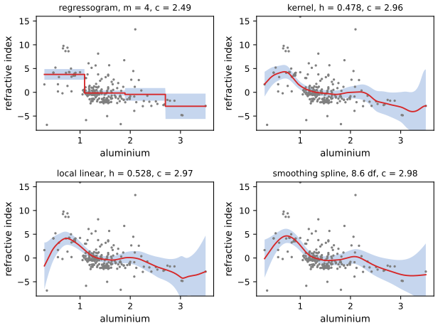
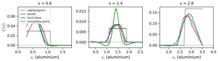

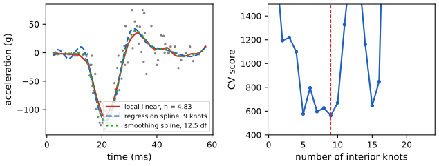
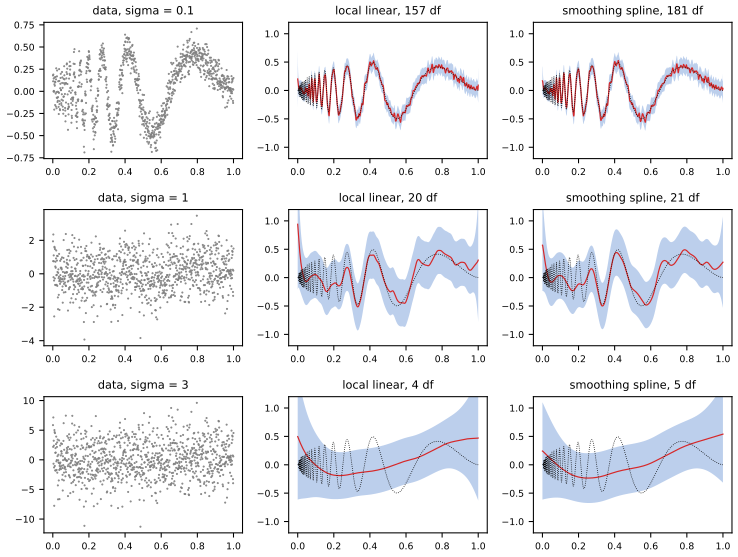
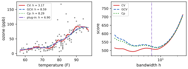
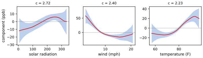
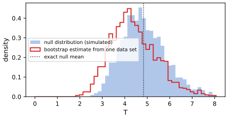
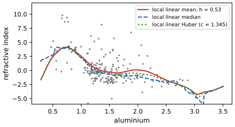
Demonstrations for this chapter
| Demonstration | What you can see | Sections and results |
|---|---|---|
| Local polynomial regression and cross-validation | Kernel (p = 0), local linear and local quadratic fits to the CMB, LIDAR, Doppler and motorcycle data; the leave-one-out and GCV scores against the degrees of freedom; the effective kernel at any point. Presets: 1 Figure 5.2; 2 two CV minima (Fig 5.3); 3 LIDAR (Fig 5.4); 4 boundary bias (Fig 5.5); 5 Doppler (Fig 5.6). | 5.3, 5.4; Theorem 5.34, 5.57, 5.60, 5.65 |
| B-splines, regression splines and smoothing splines | The Cox–de Boor recursion for any order and number of knots; regression splines (knots) and smoothing splines (\(\lambda\)) on the LIDAR, motorcycle and glass data, with their degrees of freedom and CV/GCV curves. Presets: 1 Figure 5.7; 2 orders 1 to 5 (Exercise 10); 3 smoothing spline by CV; 4 regression spline, motorcycle (Exercise 11); 5 λ to the extremes. | 5.5; Theorems 5.74, 5.76, 5.81 |
| Confidence bands and the tube formula | Local linear fits with simultaneous bands: \(\kappa_0\) and \(c\) from the tube formula, constant or estimated variance, Bonferroni over bandwidths; a simulation of the coverage of \(\br\) and of \(r\). Presets: 1 CMB, constant variance (Fig 5.11 top); 2 CMB, variance function (Fig 5.11 bottom); 3 LIDAR (Example 5.110); 4 the bias problem (Fig 5.10); 5 glass, bands across bandwidths (Exercise 9). | 5.6, 5.7, 5.9; Filling the gaps 5.14, 5.15, 5.16, 5.17 |
Related demonstrations in the companion courses: kernel regression with a band (Probability and Statistical Inference), local regression, smoothing splines and backfitting (Statistical Learning). The Python code that produces every figure of this page is code/ch05_nonparametric_regression.py (see the code index).
References
- Wasserman, L. (2006). All of Nonparametric Statistics. Springer, New York. Chapter 5, pp. 61–123. www.stat.cmu.edu/~larry/all-of-nonpar.
- Adler, R. J. and Taylor, J. E. (2007). Random Fields and Geometry. Springer, New York.
- de Boor, C. (2001). A Practical Guide to Splines, revised edition. Springer, New York.
- Breiman, L., Friedman, J. H., Olshen, R. A. and Stone, C. J. (1984). Classification and Regression Trees. Wadsworth, Belmont.
- Buja, A., Hastie, T. and Tibshirani, R. (1989). Linear smoothers and additive models. Annals of Statistics, 17, 453–555.
- Chaudhuri, P. and Marron, J. S. (1999). SiZer for exploration of structures in curves. Journal of the American Statistical Association, 94, 807–823.
- Chen, S. X. and Qin, Y. S. (2000). Empirical likelihood confidence intervals for local linear smoothers. Biometrika, 87, 946–953.
- Cramér, H. and Leadbetter, M. R. (1967). Stationary and Related Stochastic Processes. Wiley, New York.
- Craven, P. and Wahba, G. (1979). Smoothing noisy data with spline functions. Numerische Mathematik, 31, 377–403.
- Curry, H. B. and Schoenberg, I. J. (1966). On Pólya frequency functions IV: the fundamental spline functions and their limits. Journal d'Analyse Mathématique, 17, 71–107.
- Fan, J. (1992). Design-adaptive nonparametric regression. Journal of the American Statistical Association, 87, 998–1004.
- Fan, J. (1993). Local linear regression smoothers and their minimax efficiencies. Annals of Statistics, 21, 196–216.
- Fan, J. and Gijbels, I. (1996). Local Polynomial Modelling and Its Applications. Chapman and Hall, London.
- Friedman, J. H. (1991). Multivariate adaptive regression splines. Annals of Statistics, 19, 1–67.
- Friedman, J. H. and Stuetzle, W. (1981). Projection pursuit regression. Journal of the American Statistical Association, 76, 817–823.
- Gasser, T., Sroka, L. and Jennen-Steinmetz, C. (1986). Residual variance and residual pattern in nonlinear regression. Biometrika, 73, 625–633.
- Green, P. J. and Silverman, B. W. (1994). Nonparametric Regression and Generalized Linear Models. Chapman and Hall, London.
- Härdle, W., Hall, P. and Marron, J. S. (1988). How far are automatically chosen regression smoothing parameters from their optimum? Journal of the American Statistical Association, 83, 86–95.
- Härdle, W. and Mammen, E. (1993). Comparing nonparametric versus parametric regression fits. Annals of Statistics, 21, 1926–1947.
- Hastie, T., Tibshirani, R. and Friedman, J. (2001). The Elements of Statistical Learning. Springer, New York.
- Hotelling, H. (1939). Tubes and spheres in n-spaces, and a class of statistical problems. American Journal of Mathematics, 61, 440–460.
- Loader, C. (1999). Local Regression and Likelihood. Springer, New York.
- Naiman, D. Q. (1990). Volumes of tubular neighborhoods of spherical polyhedra and statistical inference. Annals of Statistics, 18, 685–716.
- Rice, J. (1984). Bandwidth choice for nonparametric regression. Annals of Statistics, 12, 1215–1230.
- Rice, S. O. (1944). Mathematical analysis of random noise. Bell System Technical Journal, 23, 282–332.
- Ruppert, D. and Wand, M. P. (1994). Multivariate locally weighted least squares regression. Annals of Statistics, 22, 1346–1370.
- Ruppert, D., Wand, M. P. and Carroll, R. J. (2003). Semiparametric Regression. Cambridge University Press.
- Scheffé, H. (1959). The Analysis of Variance. Wiley, New York.
- Silverman, B. W. (1984). Spline smoothing: the equivalent variable kernel method. Annals of Statistics, 12, 898–916.
- Stone, C. J. (1982). Optimal global rates of convergence for nonparametric regression. Annals of Statistics, 10, 1040–1053.
- Sun, J. and Loader, C. (1994). Simultaneous confidence bands for linear regression and smoothing. Annals of Statistics, 22, 1328–1345.
- Wahba, G. (1990). Spline Models for Observational Data. SIAM, Philadelphia.
The numerical statements in the text (the leave-one-out shortcut, the agreement of the B-spline and smoothing-spline implementations with library versions, the variance identities, the log-chi-square constant, the tube constants and the coverage of the bands, the minimax constant, and the numbers of the examples and exercises) were confirmed numerically.