Chapter 6. Testing
A hypothesis test turns data into a decision while controlling how often the decision is wrong when nothing is going on. This chapter starts with one test (a coin, then two groups of plants), builds the exact binomial test, the t-test and the permutation test, and shows how analysis choices made after seeing the data (p-value hacking) destroy the error guarantee. It then moves to thousands of tests at once, where the family-wise error rate is too strict and the false discovery rate takes over: the Benjamini–Hochberg procedure, the p-value histogram, the two-groups model with its local fdr, and covariates that tell us which hypotheses deserve more of the error budget. The notes follow Holmes and Huber (2019), Chapter 6, and write out every argument the book states without proof.
Ch. 1 Discrete data Ch. 2 Statistical modeling Ch. 3 Data visualization Ch. 4 Mixture models Ch. 5 Clustering Ch. 6 Testing Ch. 7 Multivariate analysis Ch. 8 Count data and GLMs Ch. 9 Heterogeneous data Ch. 10 Networks and trees Ch. 11 Image data Ch. 12 Supervised learning Ch. 13 Experimental design
How to read these notes
They follow the book. Sections carry the book's numbers (6.2, 6.9.2, ...), and displayed equations that appear in the book carry its equation numbers, e.g. (6.7). Equations without a number are steps that the book skips. The book's in-text questions are answered where they appear (Question 6.k); the end-of-chapter exercises are in Exercises.
Filling the gaps. Where the book states a result without derivation (that p-values are uniform, the null distribution of t, the exactness of permutation tests, FDR control by Benjamini–Hochberg, the estimate of the null proportion, why filtering and weighting keep the error control), an orange Filling the gap box gives the full argument. Proofs start hidden: open one with its bar, or use the button below.
Figures and demonstrations. Every figure computed from data or by simulation is reproduced from scratch by the R code. The ▶ Demo boxes open an interactive demonstration already set to the case being discussed.
Main reference
S. Holmes and W. Huber, Modern Statistics for Modern Biology, Cambridge University Press (2019), Chapter 6 (Testing). Section, equation, figure and question numbers below refer to this book. The explanations, derivations and code are my own; the book's results are cited by section, equation and figure number.
The chapter at a glance
- 6.1–6.4 A test fixes in advance a rejection region of small null probability \(\alpha\). The p-value is the null tail probability of the observed statistic; it is uniform under a continuous null and super-uniform (\(\Prob(p\le\alpha)\le\alpha\)) in general (Result 6.1). For the coin, 59 heads in 100 tosses give p = 0.0886; the test has power only 0.46 against P(head) = 0.6.
- 6.5 Under independent normal data with a common variance, \(t\) has the \(t_{n_1+n_2-2}\) distribution exactly (Result 6.3). The permutation test needs only exchangeability and is exact for every sample size (Result 6.4); on the PlantGrowth data the two p-values are 0.0469 and 0.0483. Dependence (duplicated data) inflates t by \(\sqrt{2(N-1)/(N-2)}\).
- 6.6 Testing after every new observation and stopping at the first p < 0.05 gives a false positive rate of 0.276 between n = 10 and 100, and it tends to 1 with more patience (Filling the gap 6.9).
- 6.7–6.8 With \(m_0\) true nulls tested independently at level \(\alpha\), \(\Prob(V>0)=1-(1-\alpha)^{m_0}\to1\). Bonferroni (\(\alpha/m\)) controls the FWER under any dependence (Result 6.5).
- 6.9 The FDR \(\E[V/\max(R,1)]\) is the expected fraction of false discoveries. Benjamini–Hochberg controls it at exactly \(\pi_0\varphi\) for independent tests (Result 6.6, full proof). On the airway data BH rejects 4,099 genes at \(\varphi=0.1\).
- 6.10 In the two-groups model the local fdr \(\pi_0/f(p)\) is the posterior probability that a hypothesis with p-value \(p\) is null, and the tail-area Fdr is its average over \([0,p]\) (Result 6.7).
- 6.11 A covariate independent of the p-values under the null (here the mean count) can be used to filter (4,558 BH rejections instead of 4,099) or to weight the hypotheses; weighted BH still controls the FDR (Result 6.8), and IHW finds 4,892.
Notation. \(H_0\) null hypothesis; \(T\) test statistic with observed value \(t\); \(\Prob_0\) probability under \(H_0\); \(\alpha\) significance level; \(m\) tests of which \(m_0\) are true nulls, \(\pi_0=m_0/m\); \(V,S,U,T,R\) as in Table 6.2; \(\varphi\) target FDR; \(p_{(1)}\le\dots\le p_{(m)}\) ordered p-values; \(\Phi\) the standard normal distribution function, \(z_q=\Phi^{-1}(q)\); \(\ind\{\cdot\}\) indicator.
Prerequisites. The binomial and normal distributions, sufficiency and the likelihood (book Chapters 1–2), mixture models (book Chapter 4), the empirical distribution function (book Section 3.6.7).
6.1 Goals and the setting
Section 6.1 The chapter introduces the vocabulary of testing (null hypothesis, test statistic, rejection region, p-value, types of error), shows why many tests at once are not only a burden but also a source of information, introduces the false discovery rate and its diagnostic plots, and ends with hypothesis weighting.
6.1.1 Drinking from the firehose
Section 6.1.1 Genomics routinely tests one hypothesis per position, gene or reagent: tens of thousands to billions of tests. Any procedure that is wrong with probability 5% per test will then be wrong thousands of times, so the error criterion has to change from "per test" to "per experiment" (Sections 6.7–6.9). Figure 6.1 of the book (a photograph of a screening robot) is not reproduced.
6.1.2 Testing versus classification
Section 6.1.2 Both choose between decisions from data. Classification treats the classes symmetrically and needs a model of every class. Testing is asymmetric: one state (the null, "nothing interesting") is the default, its distribution is known or can be simulated, and we only leave it when the evidence is strong. The asymmetry is the price of not modelling the alternative: we can control the error made when the null is true, but not, in general, the other one.
6.1.3 False discovery rate or p-value?
Section 6.1.3 Score every object with a number \(x\) and call a discovery when \(x\) falls left of a threshold \(c\). If the objects are a mixture of negatives (fraction \(\pi_0\), density \(f_0\)) and positives (density \(f_1\)), the four outcomes of Figure 6.2 have probabilities given by the areas left and right of \(c\). The book defines
\[ \text{FDR}=\frac{\text{area of the negatives left of } c}{\text{total area left of } c}, \tag{6.1} \] \[ \text{p-value}=\frac{\text{area of the negatives left of } c}{\text{total area of the negatives}}. \tag{6.2} \]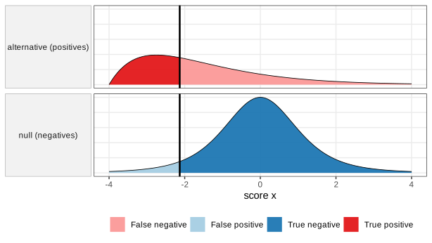
fig_6_2 in ch06_testing.R. Reproduces Holmes and Huber (2019), Figure 6.2. Download: PDF · SVG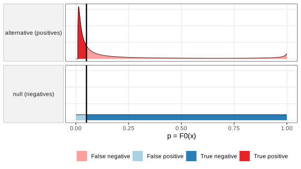
fig_6_3. Reproduces Holmes and Huber (2019), Figure 6.3. Download: PDF · SVG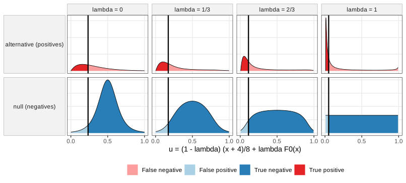
fig_6_4. Reproduces Holmes and Huber (2019), Figure 6.4. Download: PDF · SVGFilling the gap 6.1: (6.1) is a posterior probability, (6.2) a conditional probability given the null Section 6.1.3, (6.1), (6.2)
Derivation
Let \(H\in\{0,1\}\) be the class of a randomly chosen object, \(\Prob(H=0)=\pi_0\), and let \(X\given H=h\) have density \(f_h\) and distribution function \(F_h\). The marginal distribution function is \(F=\pi_0F_0+(1-\pi_0)F_1\). The light-blue area in Figure 6.2 is \(\pi_0F_0(c)\), the total area left of \(c\) is \(F(c)\), and the total null area is \(\pi_0\). Hence
\[ \text{(6.1)}=\frac{\pi_0F_0(c)}{F(c)}=\Prob(H=0\given X\le c),\qquad \text{(6.2)}=\frac{\pi_0F_0(c)}{\pi_0}=F_0(c)=\Prob(X\le c\given H=0), \]the first by Bayes' theorem. The FDR of the rule "discover when \(X\le c\)" is the probability that a discovery is a negative; the p-value of the threshold is the probability that a negative is discovered. The second needs only \(F_0\); the first also needs \(\pi_0\) and \(F_1\), the three items the book lists. If the threshold is the observed score, \(c=x\), then (6.2) is the usual p-value \(F_0(x)\) of a left-tailed test. ∎
Filling the gap 6.2: why a p-value is uniform under a continuous null, and super-uniform in general Section 6.1.3, Figure 6.3; Section 6.9.1
The book says that the transformation \(p=F_0(x)\) "always exists" and makes the null uniform, and later that null p-values are uniform "by definition" for continuous data. Here is the precise statement, including the discrete case met in Section 6.2 and in the airway p-value histogram.
Definition 6.1 (test, size, p-value)
A test of \(H_0\) is a rejection region \(\mathcal{R}\) in the sample space. Its size is \(\Prob_0(X\in\mathcal{R})\) (the supremum over all null distributions when \(H_0\) is composite); it has level \(\alpha\) if its size is at most \(\alpha\). If large values of a statistic \(T\) speak against \(H_0\), the p-value of an observed \(t\) is \(p(t)=\Prob_0(T\ge t)\). A random variable \(P\in[0,1]\) is a valid p-value if \(\Prob_0(P\le\alpha)\le\alpha\) for every \(\alpha\in[0,1]\); then "reject when \(P\le\alpha\)" is a level-\(\alpha\) test.
Result 6.1 (probability integral transform and super-uniformity)
(a) If \(X\) has a continuous distribution function \(F\), then \(F(X)\sim\Unif(0,1)\). (b) For any statistic \(T\), discrete or not, \(P=p(T)=\Prob_0(T'\ge T)\) (with \(T'\) an independent copy) satisfies \(\Prob_0(P\le\alpha)\le\alpha\) for all \(\alpha\), with equality for all \(\alpha\) when \(T\) is continuous.
Proof
(a) Let \(u\in(0,1)\). Since \(F\) is continuous with limits 0 and 1, the set \(\{x:F(x)=u\}\) is non-empty, closed and bounded above; let \(x_u\) be its largest element. As \(F\) is non-decreasing, \(X\le x_u\) implies \(F(X)\le u\), and \(X>x_u\) implies \(F(X)\ge u\) with \(F(X)\ne u\) (by maximality of \(x_u\)), so \(F(X)>u\). Hence \(\{F(X)\le u\}=\{X\le x_u\}\) and \(\Prob(F(X)\le u)=F(x_u)=u\).
(b) The survival function \(S(t)=\Prob_0(T\ge t)\) is non-increasing and left-continuous. Fix \(\alpha\) and let \(t^*=\inf\{t:S(t)\le\alpha\}\). If \(S(t^*)\le\alpha\), then \(\{S(T)\le\alpha\}=\{T\ge t^*\}\), whose probability is \(S(t^*)\le\alpha\). Otherwise \(S(t)\le\alpha\) only for \(t>t^*\), so \(\{S(T)\le\alpha\}=\{T>t^*\}\), with probability \(\lim_{t\downarrow t^*}S(t)\le\alpha\). If \(T\) is continuous, \(S=1-F_T\) is continuous and part (a) applied to \(-T\) gives equality. ∎
For a discrete statistic the inequality is usually strict, because \(\Prob_0(P\le\alpha)\) only takes the values of the attainable tail sums. For 100 tosses of a fair coin, the largest attainable size of the two-sided exact test below 0.05 is 0.0352 (we verify \(\Prob_0(P\le a)\le a\) on 220 levels). The same discreteness produces the spikes on the right of the airway p-value histogram (Figure 6.12): genes with very low counts can only produce a few, mostly large, p-values. Two-sided tests use \(T=|t|\) or, for the binomial, \(T=-\Prob_0(K=k)\) ("less probable is more extreme"), and Result 6.1(b) covers them too.
The book's point is that (6.1) answers the question we care about ("how many of my discoveries are false?") but needs the whole mixture, while (6.2) answers a less useful question but needs only the null. Multiple testing lets us estimate the missing pieces from the data (Sections 6.9–6.10).
A note on the book's text. The caption of Figure 6.3 and the sentence before (6.2) speak of "the definition of the FDR in Equation 6.2"; the FDR is Equation (6.1), and (6.2) is the p-value.
6.1.4 The multiple testing opportunity
Section 6.1.4 With one test we cannot learn \(\pi_0\) or \(f_1\). With thousands of tests the p-values themselves form a sample from the mixture, so its components can be estimated (the p-value histogram, Section 6.9.1; the two-groups model, Section 6.10), and the assumptions behind the null distribution can be checked (a flat right half of the histogram). That is why multiple testing is an opportunity.
6.2 An example: coin tossing
Section 6.2 A coin with \(\Prob(\text{head})=0.6\) is tossed \(n=100\) times; with the book's random seed the record has \(k=59\) heads. Is this enough to conclude that the coin is unfair? Under the null hypothesis of a fair coin with independent tosses, the number of heads \(K\) is binomial:
\[ \Prob(K=k\given n,p)=\binom{n}{k}p^k(1-p)^{n-k},\qquad k=0,\dots,n, \tag{6.3} \]with \(p=0.5\). Figure 6.5 plots it, Figure 6.6 approximates it by 10,000 simulated experiments.
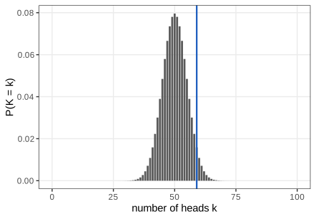
fig_6_5. Reproduces Holmes and Huber (2019), Figure 6.5. Download: PDF · SVG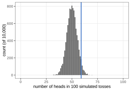
fig_6_6. Reproduces Holmes and Huber (2019), Figure 6.6. Download: PDF · SVGThe book builds the rejection region by putting values of \(k\) into it, least probable first, as long as their total null probability stays at most \(\alpha=0.05\). This gives \(\{0,\dots,40\}\cup\{61,\dots,100\}\) with size 0.0460 (Figure 6.7). The observed 59 is outside, so the fair-coin hypothesis is not rejected. R's binom.test gives the same conclusion through the p-value 0.08863 and the 95% confidence interval [0.4871, 0.6874] for \(\Prob(\text{head})\).
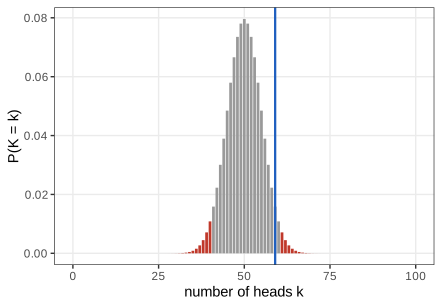
fig_6_7 and greedy_region. Reproduces Holmes and Huber (2019), Figure 6.7. Download: PDF · SVGThe Task (region from pbinom). For the symmetric fair-coin null, an equal-tailed region is \(\{0,\dots,a\}\cup\{n-a,\dots,n\}\) with the largest \(a\) such that \(2\,\Prob(K\le a)\le\alpha\). With pbinom, \(a=39\): the region is \(\{0,\dots,39\}\cup\{61,\dots,100\}\) with size 0.0352. This is exactly the set of \(k\) with binom.test p-value \(\le0.05\).
Filling the gap 6.3: the exact binomial test, its rejection region, p-value and confidence interval Section 6.2, Figure 6.7, binom.test
Derivation
The book's region is optimal for its criterion. Write \(\pi_k=\Prob_0(K=k)\). The book wants the largest number of outcomes \(|\mathcal{R}|\) subject to \(\sum_{k\in\mathcal{R}}\pi_k\le\alpha\). Any set of \(s\) outcomes has total probability at least the sum of the \(s\) smallest \(\pi_k\); so a feasible set of size \(s\) exists if and only if the \(s\) smallest are feasible, and adding outcomes in increasing order of \(\pi_k\) until the budget is exhausted attains the maximum. When two outcomes have equal probability (here \(\pi_{40}=\pi_{60}\) exactly), the order between them is arbitrary, and the budget may admit only one of them: this is the asymmetry of Figure 6.7.
The p-value of binom.test. It uses the statistic "probability of the outcome": \(p(k)=\sum_{j:\,\pi_j\le\pi_k}\pi_j\) (R allows a relative tolerance of \(10^{-7}\) in the comparison). It is valid by Result 6.1(b) applied to \(T=-\pi_K\). For \(p_0=1/2\) the pmf is symmetric and unimodal, so \(\{j:\pi_j\le\pi_k\}\)
Region and p-value. The sum defining \(p(k)\) contains every outcome that the greedy construction would add before \(k\), plus all outcomes tied with \(k\). Hence \(p(k)\le\alpha\) implies that \(k\) is in the greedy region, and the converse fails only through ties: \(k=40\) is in the book's region but \(p(40)=2\Prob(K\le40)=0.0569>0.05\). Rejecting when \(p\le\alpha\) gives the symmetric region of the Task.
Confidence interval by inversion. The 95% interval reported by binom.test (Clopper and Pearson, 1934) collects the \(p\) not rejected by either one-sided test at level 0.025: \(p_L\) solves \(\Prob_{p}(K\ge k)=0.025\) and \(p_U\) solves \(\Prob_p(K\le k)=0.025\). Differentiating in \(p\) shows the identity \(\Prob_p(K\ge k)=I_p(k,n-k+1)\), the regularised incomplete beta function: both sides vanish at \(p=0\), and
(the sum telescopes). Therefore \(p_L\) is the 0.025 quantile of Beta\((k,n-k+1)\) and \(p_U\) the 0.975 quantile of Beta\((k+1,n-k)\): for \(k=59\), [0.48714, 0.68738], as computed in R. ∎
Question 6.1
Does not rejecting the null hypothesis mean that the coin is fair?
Solution
No. Not rejecting means that the data are compatible with a fair coin, not that they rule out other coins. Here the coin is in fact biased (P(head) = 0.6), and the test detects this bias with probability only 0.462 at \(n=100\) (Filling the gap 6.4). The confidence interval [0.487, 0.687] shows how large a bias is still compatible with the data.
Question 6.2
Would more tosses give a better chance of detecting the unfair coin? How many?
Solution
Yes: the power grows with \(n\). The exact two-sided 5% test first reaches power 0.8 against P(head) = 0.6 at \(n=199\), and stays above 0.8 for all \(n\ge210\) (power is a saw-tooth in \(n\) because the attainable sizes jump). The normal approximation of Filling the gap 6.4 gives 194.
Question 6.3
Repeating the 100 tosses, might we then reject?
Solution
Yes, with probability equal to the power, 0.462 if the true P(head) is 0.6. The decision is a random variable; a single non-rejection says little when the power is low.
Question 6.4
Why is the rejection region of Figure 6.7 asymmetric (it ends at 40 on the left and starts at 61 on the right)? What other regions could be useful?
Solution
Because \(\Prob_0(K=40)=\Prob_0(K=60)=0.0108\) exactly, the two are tied in the ordering, and the sort put 40 first. After adding 40 the total is 0.0460; adding 60 would make it 0.0569 > 0.05, so 60 stays out. The construction is not invariant under the symmetry \(k\mapsto n-k\) of the problem. Alternatives: the equal-tailed region \(\{\le39\}\cup\{\ge61\}\) (size 0.0352, symmetric, the region of binom.test); a one-sided region \(\{k\ge59\}\) if only bias towards heads matters (size 0.0443); or a randomised test that rejects at \(k=40\) and \(k=60\) with probability 0.18 each, which has size exactly 0.05 (useful in theory, unpopular in practice).
Filling the gap 6.4: power and sample size for the coin Section 6.2, Questions 6.2 and 6.3; Section 6.4
Derivation
The power of a region \(\mathcal{R}\) against \(\Prob(\text{head})=p_1\) is \(\Prob_{p_1}(K\in\mathcal{R})\), an exact binomial sum: 0.462 for the symmetric 5% region at \(n=100\), \(p_1=0.6\). For a formula, use the normal approximation \(K\approx\N(np,np(1-p))\) (de Moivre–Laplace). With \(q=1-p\), the two-sided level-\(\alpha\) test rejects when \(|K-np_0|>z_{1-\alpha/2}\sqrt{np_0q_0}\). For \(p_1>p_0\) the lower tail contributes almost nothing under \(p_1\), so
\[ \text{power}\approx\Prob_{p_1}\big(K>np_0+z_{1-\alpha/2}\sqrt{np_0q_0}\big)\approx\Phi\!\left(\frac{\sqrt n(p_1-p_0)-z_{1-\alpha/2}\sqrt{p_0q_0}}{\sqrt{p_1q_1}}\right). \]Setting this equal to \(1-\beta\), i.e. the argument of \(\Phi\) to \(z_{1-\beta}\), and solving for \(n\):
\[ n\approx\left(\frac{z_{1-\alpha/2}\sqrt{p_0q_0}+z_{1-\beta}\sqrt{p_1q_1}}{p_1-p_0}\right)^2=\left(\frac{1.960\times0.5+0.842\times0.490}{0.1}\right)^2\approx193.8. \]The exact power curve (computed by binom.test's region for each \(n\)) first reaches 0.8 at \(n=199\). The sample size grows like \((p_1-p_0)^{-2}\): halving the bias to be detected quadruples the number of tosses. ∎
6.3 The five steps of hypothesis testing
Section 6.3 (1) Choose the effect of interest, the design and a test statistic; (2) set up a null hypothesis whose distribution of the statistic (the null distribution) can be computed; (3) choose the rejection region, a set of outcomes of small null probability; (4) collect the data and compute the statistic; (5) reject if the statistic falls in the region. Steps 1–3 come before the data; Section 6.6 shows what happens when they do not. The null must be both tractable and realistic: rejecting an absurdly idealised null teaches nothing. The null distribution can come from theory (the binomial, the t distribution) or from simulation or permutation (Section 6.5.1).
A test statistic only sees what it summarises: the number of heads cannot distinguish 50 tails followed by 50 heads from a well-mixed sequence, while the number of TT pairs can.
Question 6.5
What is the null distribution of the number of times two tails occur in a row?
Solution
See Filling the gap 6.5: with \(n=100\) fair independent tosses it has mean \((n-1)/4=24.75\) and variance \((5n-7)/16=30.81\), and its exact distribution follows from a two-state recursion. It is not binomial, because overlapping pairs are dependent.
Question 6.6
Would a test based on that statistic be generally preferable?
Solution
No (the book's answer). It has power against dependence between tosses, but almost none against a bias: under a biased independent coin with P(tail) = 0.4 the TT count has mean \(99\times0.16=15.8\), but its noise is larger than that of the head count, and it uses only part of the information about the bias. Each statistic is good against its own class of alternatives.
Question 6.7
Is the number of heads a sufficient statistic for the binomial distribution? Why is it good against the first class of alternatives but not the second?
Solution
Yes; see Filling the gap 6.5. For independent tosses with unknown P(head) the likelihood depends on the data only through \(k\), and among tests of \(p=1/2\) against \(p>1/2\) the one rejecting for large \(k\) is uniformly most powerful (Result 6.2). When tosses are correlated with P(head) still 1/2, the likelihood depends on the order of the outcomes, \(k\) is no longer sufficient, and \(K\) has the same mean as under the null, so a test based on \(K\) has little power.
Filling the gap 6.5: the TT-pair statistic, sufficiency and the best test against a bias Section 6.3, Questions 6.5–6.7
Derivation
Moments of the TT count. Let \(X_1,\dots,X_n\) be independent fair tosses and \(I_j=\ind\{X_j=X_{j+1}=\mathrm{T}\}\), \(j=1,\dots,n-1\), \(W=\sum_jI_j\). Then \(\E I_j=1/4\), so \(\E W=(n-1)/4\). Also \(\var I_j=\tfrac14\cdot\tfrac34=\tfrac3{16}\); neighbouring indicators share one toss, \(\E[I_jI_{j+1}]=\Prob(\mathrm{TTT})=\tfrac18\), so \(\cov(I_j,I_{j+1})=\tfrac18-\tfrac1{16}=\tfrac1{16}\); indicators further apart are independent. Hence
\[ \var W=(n-1)\tfrac{3}{16}+2(n-2)\tfrac{1}{16}=\frac{5n-7}{16}. \]Exact distribution. Let \(a_i(w,s)\) be the probability that the first \(i\) tosses contain \(w\) TT pairs and end with \(s\in\{\mathrm H,\mathrm T\}\). Then \(a_1(0,\cdot)=\tfrac12\) and \(a_{i+1}(w,\mathrm H)=\tfrac12[a_i(w,\mathrm H)+a_i(w,\mathrm T)]\), \(a_{i+1}(w,\mathrm T)=\tfrac12[a_i(w,\mathrm H)+a_i(w-1,\mathrm T)]\); \(\Prob(W=w)=a_n(w,\mathrm H)+a_n(w,\mathrm T)\). This distribution has the two moments above.
Sufficiency. For independent tosses with \(\Prob(\mathrm H)=p\) the likelihood is \(p^k(1-p)^{n-k}\), a function of \(k\) only; by the factorisation theorem \(K\) is sufficient: given \(K=k\), every ordering is equally likely, whatever \(p\).
Result 6.2 (Neyman–Pearson for the coin)
Among all tests of \(p=p_0\) with size at most \(\alpha\), the test that rejects for large \(k\) (randomising at the boundary to attain size exactly \(\alpha\)) has the largest power against every \(p_1>p_0\).
Proof
For a simple alternative \(p_1\), let \(\phi^*\) reject when \(L(k)=\Prob_{p_1}(K=k)/\Prob_{p_0}(K=k)>c\) (randomising when \(L=c\)) with size \(\alpha\), and let \(\phi\) be any test (a function of the data with values in [0,1]) of size \(\le\alpha\). Since \((\phi^*-\phi)(\Prob_{p_1}-c\Prob_{p_0})\ge0\) pointwise (both factors have the same sign), summing over outcomes gives \(\E_{p_1}\phi^*-\E_{p_1}\phi\ge c(\E_{p_0}\phi^*-\E_{p_0}\phi)\ge0\). Here \(L(k)=(p_1q_0/(p_0q_1))^k(q_1/q_0)^n\) is increasing in \(k\) when \(p_1>p_0\), so \(\phi^*\) rejects for large \(k\), and the region does not depend on \(p_1\). It is therefore most powerful against every \(p_1>p_0\) at once. ∎
Against two-sided alternatives no uniformly most powerful test exists (the best region for \(p_1>p_0\) is the upper tail, for \(p_1<p_0\) the lower tail), which is why two-sided tests split \(\alpha\) between the tails. ∎
6.3.1 The rejection region
Section 6.3.1 The size of the region is the significance level \(\alpha\), the probability of rejecting a true null; 0.05 is a convention, not a law (Wasserstein and Lazar, 2016). The shape should maximise the power against the alternatives we care about. Without knowledge of the alternative, the book maximises the number of outcomes in the region; with a direction in mind (bias towards heads), all of \(\alpha\) goes into one tail (Result 6.2). These are one-sided and two-sided tests.
6.4 Types of error
Section 6.4, Table 6.1
| Test versus reality | Null hypothesis is true | Null hypothesis is false |
|---|---|---|
| Reject | Type I error (false positive) | True positive |
| Do not reject | True negative | Type II error (false negative) |
The false positive rate is \(\alpha\) (1 − \(\alpha\) is the specificity); the false negative rate is \(\beta\), and \(1-\beta\) is the power (sensitivity, true positive rate). Moving the threshold in Figure 6.2 trades one error for the other: for fixed data, a smaller \(\alpha\) means a smaller region and hence lower power. The only way to reduce both is more information: more or better data, or a statistic better matched to the alternative.
Question 6.8
Why distinguish one- and two-sided tests? Why not always use the two-sided test, which detects more alternatives?
Solution
Because the two-sided test pays for its breadth with power: it spends only \(\alpha/2\) in each tail. If the direction of the effect is known in advance (a drug can only help, a knockout can only reduce expression), the one-sided test is more powerful against the alternatives that matter (59 heads: one-sided p = 0.044, two-sided 0.089), and by Result 6.2 it is the best possible against them. The direction must be fixed before seeing the data; choosing it afterwards doubles the real type I error.
6.5 The t-test
Section 6.5 For two groups of measurements, the two-sample t statistic is
\[ t=c\,\frac{m_1-m_2}{s}, \tag{6.4} \]with group means \(m_g\), pooled standard deviation \(s\) and a constant depending on the sample sizes:
\[ m_g=\frac1{n_g}\sum_{i=1}^{n_g}x_{g,i},\qquad s^2=\frac{\sum_{i=1}^{n_1}(x_{1,i}-m_1)^2+\sum_{j=1}^{n_2}(x_{2,j}-m_2)^2}{n_1+n_2-2},\qquad c=\sqrt{\frac{n_1n_2}{n_1+n_2}}. \tag{6.5} \]On R's PlantGrowth data (Figure 6.8), the control (mean 5.032) against treatment 2 (mean 5.526) gives \(t=-2.134\) with 18 degrees of freedom and p = 0.04685.
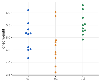
PlantGrowth data. Code: fig_6_8. Reproduces Holmes and Huber (2019), Figure 6.8. Download: PDF · SVGFilling the gap 6.6: the null distribution of t Section 6.5, (6.4), (6.5)
The book says that t.test uses "the asymptotic theory" of \(t\). Under its assumptions the t distribution is in fact the exact null distribution for every sample size; nothing asymptotic is involved.
Result 6.3 (Student's t)
Let \(x_{1,1},\dots,x_{1,n_1},x_{2,1},\dots,x_{2,n_2}\) be independent, \(x_{g,i}\sim\N(\mu_g,\sigma^2)\) with a common \(\sigma^2\), and \(N=n_1+n_2\). If \(\mu_1=\mu_2\), then \(t\) in (6.4) has the t distribution with \(\nu=N-2\) degrees of freedom, with density
\[ f_\nu(t)=\frac{\Gamma\big(\frac{\nu+1}2\big)}{\sqrt{\nu\pi}\,\Gamma\big(\frac\nu2\big)}\Big(1+\frac{t^2}\nu\Big)^{-(\nu+1)/2}. \]Proof
Step 1: within one group, the mean and the sum of squares are independent. Take \(n\) independent \(\N(\mu,\sigma^2)\) values, put \(y=(x-\mu\mathbf 1)/\sigma\sim\N(\mathbf0,\mathbf I_n)\), and let \(Q\) be an orthogonal matrix whose first row is \(\mathbf1^\T/\sqrt n\). Then \(w=Qy\sim\N(\mathbf0,QQ^\T)=\N(\mathbf0,\mathbf I_n)\): its coordinates are independent standard normals. Here \(w_1=\sqrt n(\bar x-\mu)/\sigma\), and \(\sum_{i\ge2}w_i^2\)
Step 2: numerator. \(m_1-m_2\sim\N\big(0,\sigma^2(\tfrac1{n_1}+\tfrac1{n_2})\big)\) and \(\tfrac1{n_1}+\tfrac1{n_2}=\tfrac{N}{n_1n_2}=c^{-2}\), so \(Z=c(m_1-m_2)/\sigma\sim\N(0,1)\). This is where \(c\) comes from.
Step 3: denominator. \(V=(N-2)s^2/\sigma^2=\mathrm{SS}_1/\sigma^2+\mathrm{SS}_2/\sigma^2\) is a sum of independent \(\chi^2_{n_1-1}\) and \(\chi^2_{n_2-1}\) variables, so \(V\sim\chi^2_\nu\). By Step 1 and the independence of the groups, \(V\) is independent of \((m_1,m_2)\), hence of \(Z\).
Step 4: the ratio. \(t=Z/\sqrt{V/\nu}\). Conditionally on \(V=v\), \(t\sim\N(0,\nu/v)\), so with \(g_\nu(v)=v^{\nu/2-1}e^{-v/2}/(2^{\nu/2}\Gamma(\nu/2))\),
\[ f(t)=\int_0^\infty\sqrt{\tfrac{v}{2\pi\nu}}\,e^{-t^2v/(2\nu)}g_\nu(v)\,\d v=\frac{1}{\sqrt{2\pi\nu}\,2^{\nu/2}\Gamma(\frac\nu2)}\int_0^\infty v^{\frac{\nu+1}2-1}e^{-\frac v2(1+\frac{t^2}\nu)}\d v. \]The last integral is a gamma integral, \(\Gamma(\frac{\nu+1}2)\big(\tfrac12(1+t^2/\nu)\big)^{-(\nu+1)/2}\); collecting the powers of 2 gives the density above. ∎
What the result needs: independence, normality, a common variance. Normality is the least important for moderate samples (the numerator is approximately normal by the central limit theorem and \(s^2\) converges to \(\sigma^2\)); independence is the most important (Filling the gap 6.7). With unequal variances, Welch's statistic \((m_1-m_2)/\sqrt{s_1^2/n_1+s_2^2/n_2}\) with Satterthwaite's degrees of freedom is the usual approximation; with \(n_1=n_2\) the two statistics are identical (both denominators equal \(\sqrt{(s_1^2+s_2^2)/n}\)), only the degrees of freedom differ (16.8 instead of 18 here).
Question 6.9
What do you get for ctrl versus trt1, and trt1 versus trt2?
Solution
ctrl versus trt1: \(t=1.191\), p = 0.249 (exact permutation p = 0.248). trt1 versus trt2: \(t=-3.010\), p = 0.0075 (permutation p = 0.0086). Only the two treatments differ clearly; note that three pairwise tests are already a small multiple-testing problem (Section 6.7).
Question 6.10
Plot the theoretical and simulated null distributions of the t statistic, as for the coin.
Solution
Figures 6.9 and 6.10. Instead of 10,000 random relabellings, Figure 6.9 uses all \(\binom{20}{10}=184{,}756\) splits of the 20 plants into two groups of ten, i.e. the exact permutation distribution. The 2.5% and 97.5% quantiles of the two distributions are close, and the two-sided p-values agree to within 0.0015.
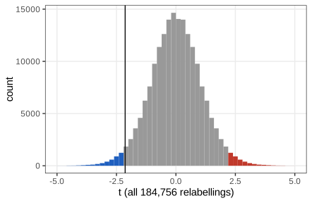
fig_6_9 and perm_t_all. Reproduces Holmes and Huber (2019), Figure 6.9. Download: PDF · SVG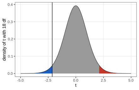
fig_6_10. Reproduces Holmes and Huber (2019), Figure 6.10. Download: PDF · SVGQuestion 6.11
Would it be simpler to work with \(|t|\)?
Solution
Yes (the book's answer): a two-sided test is a one-sided test on \(|t|\), with a single upper rejection region. The one-sided test in the direction of the data halves the p-value when the null distribution is symmetric: 0.0234 (t distribution) and 0.0242 (exact permutation).
Flavours. The test above is two-sided, two-sample, unpaired, with equal variances. A one-sample test compares one mean with a fixed number; a paired test analyses within-unit differences (one-sample test on the differences); Welch's test drops the equal-variance assumption.
The independence assumption. Entering every plant twice leaves the means unchanged but gives \(t=-3.1007\) on 38 degrees of freedom, p = 0.0036.
Filling the gap 6.7: what duplication and pseudo-replication do to t Section 6.5, duplicated PlantGrowth data
Derivation
Copy each of the \(N=n_1+n_2\) observations \(r\) times. The means do not change; each within-group sum of squares is multiplied by \(r\); the degrees of freedom become \(rN-2\); and \(c\) becomes \(\sqrt{r^2n_1n_2/(rN)}=\sqrt r\,c\). Hence, with \(d=m_1-m_2\) and \(\mathrm{SS}=\mathrm{SS}_1+\mathrm{SS}_2\),
\[ t_r=\frac{\sqrt r\,c\,d}{\sqrt{r\,\mathrm{SS}/(rN-2)}}=t\sqrt{\frac{rN-2}{N-2}}. \]For \(r=2\), \(N=20\): \(t_2=t\sqrt{38/18}=-3.1007\), exactly the book's output. As \(r\to\infty\), \(|t_r|\to\infty\) and the p-value goes to 0, although no information was added. The t-test believes it sees \(rN\) independent values.
Technical replicates. More realistically, each of \(n\) plants per group is measured \(k\) times with correlation \(\rho\) between measurements of the same plant. A plant mean then has variance \(\sigma^2(1+(k-1)\rho)/k\) (the design effect), but the naive test uses \(\sigma^2/k\). In large samples the naive statistic is approximately \(\N(0,1+(k-1)\rho)\) under the null, so its true size is about \(2\Phi\big(-z_{0.975}/\sqrt{1+(k-1)\rho}\big)\): 0.17 for \(k=2,\rho=1\). The correct analysis averages the replicates within each plant (or uses a mixed model), which brings back an exact t-test with \(2n-2\) degrees of freedom. Exercise 6.3 simulates the small-sample case. ∎
6.5.1 Permutation tests
Section 6.5.1 The permutation test uses the same statistic \(t\) but a different null distribution: the values of \(t\) over all relabellings of the pooled observations. Its only assumption is that, under the null, the labels are exchangeable: the joint distribution of the \(N\) observations does not change when they are permuted. This is weaker than the t-test's assumption (independent, identically distributed normal values are exchangeable, but so are many non-normal ones), and the permutation null distribution is discrete, with at most \(\binom{N}{n_1}\) distinct values (the book's \(N!\) permutations give each split \(n_1!\,n_2!\) times).
Algorithm 6.1 (permutation test, exact and Monte Carlo)
- Compute the statistic on the data: \(t_0=T(z)\), with \(z\) the pooled observations in their original order (the first \(n_1\) are group 1).
- Exact: for every subset of \(n_1\) positions, relabel those as group 1 and compute \(T\); \(p=\#\{\text{splits with }|T|\ge|t_0|\}/\binom N{n_1}\).
- Monte Carlo: draw \(B\) random permutations \(\pi_1,\dots,\pi_B\), compute \(T(z\circ\pi_b)\), and report \(p=(1+b)/(B+1)\) with \(b=\#\{b:|T(z\circ\pi_b)|\ge|t_0|\}\).
Filling the gap 6.8: permutation tests are exact; t and the difference of means give the same test Section 6.5.1
Result 6.4 (exactness of permutation tests)
Let \(G\) be the group of all permutations of the \(N\) positions and suppose that under \(H_0\) the vector \(Z\) is exchangeable: \(Z\circ\pi\) has the distribution of \(Z\) for every \(\pi\in G\). Then (a) the exact p-value \(p(Z)\)
Proof
(a) Fix a data vector \(z\). Because \(\sigma\pi\) runs through \(G\) when \(\pi\) does, \(p(z\circ\sigma)\)
(b) Let \(\pi_0\) be the identity and \(\pi_1,\dots,\pi_B\) independent uniform draws from \(G\). Take \(\eta\) uniform on \(G\), independent of everything; under \(H_0\), \(W=Z\circ\eta^{-1}\) has the distribution of \(Z\) and is independent of \(\eta\) (by exchangeability, conditionally on \(\eta\) the law of \(W\) is the null law). Then \(Z\circ\pi_b=W\circ(\eta\pi_b)\), and given \(W\) the \(B+1\) permutations \(\eta\pi_0,\dots,\eta\pi_B\) are independent and uniform on \(G\). So, given \(W\), the values \(T_b=T(Z\circ\pi_b)\), \(b=0,\dots,B\), are exchangeable, and the rank of \(T_0\) among them (counting ties against us) is at least uniform: \(\Prob(1+\#\{b\ge1:T_b\ge T_0\}\le j)\)
t versus the difference of means. For fixed pooled data, the total sum of squares \(\mathrm{SS}_\text{tot}=\sum(z_i-\bar z)^2\) is the same for every relabelling, and the within-group sum of squares is \(\mathrm{SS}_\text{tot}-\tfrac{n_1n_2}{N}D^2\) with \(D=m_1-m_2\). Therefore
\[ t=\frac{cD}{\sqrt{(\mathrm{SS}_\text{tot}-c^2D^2)/(N-2)}}, \]a strictly increasing function of \(D\) on its range: the permutation tests based on \(t\) and on \(D\) reject exactly the same relabellings and give identical p-values (the demo shows both). Over the relabellings, \(D\) has mean 0 and variance \(S^2(\tfrac1{n_1}+\tfrac1{n_2})\), where \(S^2=\mathrm{SS}_\text{tot}/(N-1)\); this follows from sampling without replacement: \(D=\tfrac{N}{n_2}(m_1-\bar z)\) and \(\var(m_1)=\tfrac{S^2}{n_1}\big(1-\tfrac{n_1}{N}\big)\). The permutation distribution of \(D/\sqrt{S^2(1/n_1+1/n_2)}\) is approximately standard normal for large groups (the combinatorial central limit theorem, Hoeffding 1951), which is why the permutation and t p-values agree so well; the book's "consequence of the Central Limit Theorem" refers to this.
On the PlantGrowth data the exact permutation p-value is 0.04833 against 0.04685 from the t distribution. The two tests are different tests whose answers happen to agree, because the data are roughly normal and the groups balanced.
6.6 P-value hacking
Section 6.6 Every analysis choice made after seeing the data (another test statistic, another normalisation, removing an "outlier", testing again after a few more observations) is a new chance for a null effect to cross the 5% line. Trying until something works is p-value hacking; changing the hypothesis after seeing the results is HARKing (Head et al., 2015). The guarantee \(\Prob_0(p\le\alpha)\le\alpha\) holds for a procedure fixed in advance, not for the minimum over several procedures. The remedy the book recommends is transparency: report everything that was tried, and publish the code.
Also, a large p-value does not show that the null is true: a test of a meaningless null with a tiny sample gives a p-value that is essentially a random number and "confirms" anything.
Filling the gap 6.9: how much optional stopping and statistic shopping cost Section 6.6
Derivation
Best of K statistics. If \(K\) independent valid p-values are computed and the smallest is reported, \(\Prob_0(\min_jP_j\le\alpha)=1-(1-\alpha)^K\): 0.226 for \(K=5\). Statistics computed from the same data are usually positively correlated, which helps but does not cure: for \(K\) equicorrelated normal statistics \(Z_j=\sqrt\rho\,U+\sqrt{1-\rho}\,E_j\) (independent standard normal \(U,E_j\)), conditioning on \(U\) makes them independent, so
\[ \Prob_0\big(\max_j|Z_j|\le z_{1-\alpha/2}\big)=\int\varphi(u)\Big[\Phi\Big(\frac{z_{1-\alpha/2}-\sqrt\rho u}{\sqrt{1-\rho}}\Big)-\Phi\Big(\frac{-z_{1-\alpha/2}-\sqrt\rho u}{\sqrt{1-\rho}}\Big)\Big]^K\d u, \]which gives a false positive rate of 0.127 for \(K=5\), \(\rho=0.8\) (checked against simulation).
Optional stopping. Observe \(X_1,X_2,\dots\) independent \(\N(0,1)\) (the null), \(S_n=X_1+\dots+X_n\), and test \(|S_n|/\sqrt n>z_{0.975}\) after each new observation, stopping at the first rejection. Each single test has size 0.05, but the probability that at least one of the looks \(n_0,\dots,n_\text{max}\) rejects is much larger. It can be computed exactly (Armitage, McPherson and Rowe, 1969): let \(g_j\) be the sub-density of \(S_{n_j}\) on the paths that have not stopped before look \(j\). Then \(g_1\) is the \(\N(0,n_1)\) density, and
\[ g_{j+1}(s)=\int_{|u|\le z\sqrt{n_j}}g_j(u)\,\frac{1}{\sqrt{n_{j+1}-n_j}}\varphi\Big(\frac{s-u}{\sqrt{n_{j+1}-n_j}}\Big)\d u,\qquad \Prob(\text{stop at look }j)=\int_{|s|>z\sqrt{n_j}}g_j(s)\,\d s, \]because between looks the increment \(S_{n_{j+1}}-S_{n_j}\sim\N(0,n_{j+1}-n_j)\) is independent of the past. The R function optional_stopping_exact and the demo evaluate this on a grid (cell width 0.05, convolution, partial absorption of boundary cells; halving the cell width changes the result by \(2\times10^{-5}\)). Looking after every observation from 10 to 100 gives a false positive rate of 0.2764 (simulation: 0.2816 ± 0.0032); looking every 10 observations, 0.1934; every observation up to 1,000, 0.4571.
With enough patience, every null is rejected. By the law of the iterated logarithm, \(\limsup_n S_n/\sqrt{2n\log\log n}=1\) almost surely, so \(|S_n|/\sqrt n\) exceeds any fixed \(z\) for infinitely many \(n\), with probability 1. The false positive rate of "test until significant" tends to 1. Sequential designs that are allowed to look repeatedly (group-sequential boundaries of Pocock or O'Brien and Fleming, or anytime-valid tests) use boundaries that grow with the number of looks. ∎
6.7 Multiple testing
Section 6.7, Table 6.2 With \(m\) hypotheses, the outcomes of Table 6.1 become counts:
| Test versus reality | Null is true | Null is false | Total |
|---|---|---|---|
| Rejected | \(V\) | \(S\) | \(R\) |
| Not rejected | \(U\) | \(T\) | \(m-R\) |
| Total | \(m_0\) | \(m-m_0\) | \(m\) |
Only \(m\) and \(R\) are observed; \(V,S,U,T\) and \(m_0\) are not.
Definition 6.2 (error rates for many tests) Sections 6.8, 6.9, (6.7)
The family-wise error rate is \(\FWER=\Prob(V>0)\). The false discovery proportion is \(\FDP=V/\max(R,1)\) (0 when nothing is rejected) and the false discovery rate is its expectation \(\FDR=\E[\FDP]\). A procedure controls an error rate at level \(q\) if the rate is at most \(q\) whatever the configuration of true and false nulls (strong control); weak control requires this only when all nulls are true.
Question 6.12
In the jelly-bean cartoon (xkcd 882), why does the newspaper not report the other colours?
Solution
Twenty colours were tested at 5%; even with no effect at all, \(\Prob(\text{at least one }p\le0.05)=1-0.95^{20}=0.64\). The one "significant" colour is reported because it was significant, so the selection guarantees an exciting headline and hides the 19 other tests that make it unremarkable. Without the denominator (how many tests were done), a p-value cannot be interpreted.
6.8 The family wise error rate
Section 6.8 If the \(m_0\) true nulls are tested independently, each at level \(\alpha\) with exactly uniform p-values,
\[ \Prob(V>0)=1-\Prob(\text{no rejection among the }m_0\text{ nulls})=1-(1-\alpha)^{m_0}\;\to\;1\quad(m_0\to\infty). \tag{6.6} \]A DNA profile with a one-in-a-million chance of a random match, searched against 800,000 unrelated profiles, gives \(1-(1-10^{-6})^{8\times10^5}=0.551\): a random hit is more likely than not.
Question 6.13
Show that (6.6) becomes very close to 1 when \(m_0\) is large.
Solution
Since \(1-x\le e^{-x}\) for all \(x\) (the exponential is convex and \(1-x\) is its tangent at 0), \((1-\alpha)^{m_0}\le e^{-\alpha m_0}\), so \(1-(1-\alpha)^{m_0}\ge1-e^{-\alpha m_0}\to1\). The bound is already close to 1 when \(m_0\) is a few times \(1/\alpha\): \(1-e^{-3}=0.95\) at \(m_0=3/\alpha\). For the DNA example, \(1-e^{-0.8}=0.551\), matching the exact value to three digits.
6.8.1 Bonferroni method
Section 6.8.1 To control the FWER at \(\alpha_\text{FWER}\), test each hypothesis at \(\alpha=\alpha_\text{FWER}/m\). Figure 6.11 plots (6.6) for \(m=10{,}000\) against the per-test level: the curve reaches 0.05 at \(\alpha=5.13\times10^{-6}\), slightly above \(0.05/m=5\times10^{-6}\).
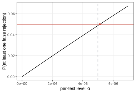
fig_6_11. Reproduces Holmes and Huber (2019), Figure 6.11. Download: PDF · SVGFilling the gap 6.10: Bonferroni needs no independence; Šidák is the exact level under independence Section 6.8.1, Question 6.14
Result 6.5 (Bonferroni and Šidák)
(a) If every true-null p-value is valid, rejecting \(p_i\le\alpha/m\) gives \(\FWER\le m_0\alpha/m\le\alpha\), under any dependence between the tests. (b) If the \(m_0\) null p-values are independent and uniform, rejecting \(p_i\le1-(1-\alpha)^{1/m}\) gives \(\FWER=1-(1-\alpha)^{m_0/m}\le\alpha\), with equality when \(m_0=m\), and \(1-(1-\alpha)^{1/m}\ge\alpha/m\).
Proof
(a) By the union bound, \(\Prob(V>0)\)
This answers Question 6.14: the crossing point of Figure 6.11 is the Šidák level, which is exact for independent tests, while Bonferroni's \(\alpha/m\) is a bound valid for any dependence and therefore slightly smaller (\(5.129\times10^{-6}\) versus \(5\times10^{-6}\)). Simulated with 20 equicorrelated tests (\(\rho=0.5\)), Bonferroni has FWER 0.040 < 0.05: positive dependence makes it conservative. Holm's step-down procedure (see Exercise 6.5) is uniformly more powerful than Bonferroni with the same guarantee.
The cost is power: at \(\alpha/m=5\times10^{-6}\) each test needs a very strong signal. With the airway data below, Bonferroni at 0.1 rejects 1,444 genes against 4,099 for Benjamini–Hochberg.
6.9 The false discovery rate
Section 6.9 The airway data (Himes et al., 2014) contain RNA-Seq counts of four human airway smooth muscle cell lines, each treated and untreated with dexamethasone. DESeq2 (Love, Huber and Anders, 2014; book Chapter 8) fits a model with cell line and treatment and tests each gene for a treatment effect; 33,469 genes get a p-value.
6.9.1 The p-value histogram
Section 6.9.1 The histogram of all p-values (Figure 6.12) is the first diagnostic of any multiple-testing analysis. It is a mixture of the null p-values, uniform when the null distribution is right (Result 6.1), and the alternative p-values, concentrated near 0 when the tests have power, with a shoulder to the right when some have little power.
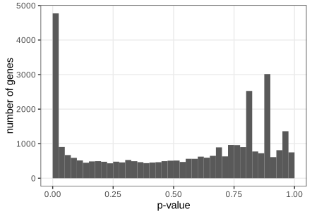
fig_6_12 and airway_results. Reproduces Holmes and Huber (2019), Figure 6.12. Download: PDF · SVGIf we reject all p-values in the first bin \([0,0.025]\), we make 4,772 rejections. The book estimates the null proportion by \(\hat\pi_0=2\times\#\{p>0.5\}/m\), which gives an expected \(\hat\pi_0\,m\times0.025=945\) nulls in the bin (blue line of Figure 6.13) and an estimated false discovery proportion of 945/4,772 = 0.198.
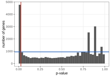
fig_6_13. Reproduces Holmes and Huber (2019), Figure 6.13. Download: PDF · SVGThe book then defines (Definition 6.2)
\[ \FDR=\E\left[\frac{V}{\max(R,1)}\right]. \tag{6.7} \]The FDR is an average over hypothetical repetitions of the experiment; the realised \(\FDP=v/r\) of one experiment can be larger or smaller.
Filling the gap 6.11: FDR versus FWER Section 6.9.1, (6.7)
Derivation
Pointwise, \(V/\max(R,1)\le\ind\{V>0\}\) (if \(V=0\) both are 0; otherwise the left side is at most 1). Taking expectations, \(\FDR\le\FWER\): every FWER-controlling procedure controls the FDR, and FDR control is the weaker requirement, which buys power. If all nulls are true, then \(S=0\), \(V=R\) and \(V/\max(R,1)=\ind\{V>0\}\), so \(\FDR=\FWER\): FDR control implies weak FWER control. When many hypotheses are false, \(R\) is large and a few false rejections cost little FDR, so an FDR procedure can afford a much larger threshold. ∎
Filling the gap 6.12: the estimate of \(\pi_0\), why it is conservative, and why it exceeds 1 here Section 6.9.1, Figure 6.13
Derivation
Fix \(\lambda\in(0,1)\) and let \(W(\lambda)=\#\{i:p_i>\lambda\}\). If the null p-values are uniform,
\[ \E W(\lambda)=\sum_{i\in\mathcal H_0}\Prob(p_i>\lambda)+\sum_{i\notin\mathcal H_0}\Prob(p_i>\lambda)=m_0(1-\lambda)+\sum_{i\notin\mathcal H_0}\Prob(p_i>\lambda)\ \ge\ m_0(1-\lambda), \]so \(\hat\pi_0(\lambda)=W(\lambda)/(m(1-\lambda))\) satisfies \(\E\hat\pi_0(\lambda)\ge\pi_0\) (Storey, 2002). The bias \(\sum_{\text{alt}}\Prob(p_i>\lambda)/(m(1-\lambda))\) is small when the alternatives rarely give large p-values; larger \(\lambda\) reduces the bias and increases the variance. The book's choice \(\lambda=1/2\) gives \(2\#\{p>0.5\}/m\). (Simulation: with \(\pi_0=0.8\) and weak alternatives, the average estimate is 0.864.) The visual FDR estimate of a threshold \(t\) is \(\hat\pi_0\,m\,t/R(t)\), where \(R(t)=\#\{p_i\le t\}\): expected number of null p-values below \(t\) divided by the observed number.
The airway estimate is 1.129. On these data \(2\#\{p>0.5\}/m=1.129\): more than all the genes would be null, which is impossible for a proportion. The reason is the spikes of Figure 6.12: low-count genes have super-uniform null p-values (Filling the gap 6.2), concentrated near 1, so \(\Prob(p_i>\lambda)>1-\lambda\) for them and the estimator, still conservative, overshoots. The book uses this value without comment; capping at 1 gives an estimated FDR of 0.175 instead of 0.198. Restricting to the 22,853 genes with baseMean \(\ge1\) removes most of the discreteness and gives \(\hat\pi_0(0.5)=0.762\), consistent with the Schweder–Spjøtvoll estimate below. ∎
6.9.2 The Benjamini–Hochberg algorithm for controlling the FDR
Section 6.9.2
Algorithm 6.2 (Benjamini and Hochberg, 1995) Section 6.9.2
- Order the p-values: \(p_{(1)}\le p_{(2)}\le\dots\le p_{(m)}\).
- For the target FDR \(\varphi\), find \(k=\max\{i:p_{(i)}\le\varphi\,i/m\}\) (\(k=0\) if there is none).
- Reject the hypotheses with the \(k\) smallest p-values, i.e. all \(i\) with \(p_i\le\varphi k/m\).
Graphically (Figure 6.14), BH finds the last crossing of the sorted p-values with the line of slope \(\varphi/m\). On the airway data with \(\varphi=0.1\), \(k=4{,}099\), i.e. all genes with \(p\le0.01225\).
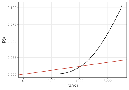
fig_6_14 and bh_k. Reproduces Holmes and Huber (2019), Figure 6.14. Download: PDF · SVGResult 6.6 (BH controls the FDR) Section 6.9.2; Benjamini and Hochberg (1995)
Suppose the null p-values are independent and uniform on \([0,1]\), and independent of the non-null p-values (which may have any joint distribution). Then the BH procedure at level \(\varphi\) has
\[ \FDR=\frac{m_0}{m}\,\varphi=\pi_0\varphi\le\varphi. \]If the null p-values are only super-uniform (valid but not exactly uniform), \(\FDR\le\pi_0\varphi\).
Proof
Notation. For \(t\in[0,1]\) let \(N(t)=\#\{j:p_j\le t\}\). The BH count is \(R=\max\{k\ge1:N(\varphi k/m)\ge k\}\) (0 if the set is empty): indeed \(p_{(k)}\le\varphi k/m\) if and only if at least \(k\) p-values are \(\le\varphi k/m\). The rejected set is \(\{j:p_j\le\varphi R/m\}\). Since \(R\le m\) and \(V=\sum_{i\in\mathcal H_0}\ind\{p_i\le\varphi R/m\}\),
\[ \frac{V}{\max(R,1)}=\sum_{i\in\mathcal H_0}\sum_{k=1}^m\frac{\ind\{R=k\}\,\ind\{p_i\le\varphi k/m\}}{k}. \]Lemma (leave-one-out). For \(i\) fixed, let \(R^{(i)}\) be the BH count computed after replacing \(p_i\) by 0; it is a function of the other p-values only. Then, on the event \(\{p_i\le\varphi k/m\}\), \(R=k\) if and only if \(R^{(i)}=k\).
Proof of the lemma. Let \(N^{(i)}(t)\) be the count with \(p_i\) replaced by 0, so \(N^{(i)}(t)=N(t)+\ind\{p_i>t\}\). If \(p_i\le\varphi k/m\), then for every \(k'\ge k\) we have \(p_i\le\varphi k'/m\), hence \(N^{(i)}(\varphi k'/m)=N(\varphi k'/m)\). Both \(R=k\) and \(R^{(i)}=k\) are statements about the counts at \(\varphi k'/m\) for \(k'\ge k\) only ("at least \(k\) at \(k'=k\), fewer than \(k'\) at every \(k'>k\)"), and these counts agree. So the two events coincide.
Main step. Using the lemma, then the independence of \(p_i\) from \(R^{(i)}\) and \(\Prob(p_i\le\varphi k/m)=\varphi k/m\):
\[ \E\big[\ind\{R=k\}\ind\{p_i\le\varphi k/m\}\big]=\E\big[\ind\{R^{(i)}=k\}\ind\{p_i\le\varphi k/m\}\big]=\frac{\varphi k}{m}\,\Prob(R^{(i)}=k). \]Dividing by \(k\) and summing over \(k\):
\[ \FDR=\sum_{i\in\mathcal H_0}\frac{\varphi}{m}\sum_{k=1}^m\Prob(R^{(i)}=k)=\sum_{i\in\mathcal H_0}\frac{\varphi}{m}=\frac{m_0}{m}\varphi, \]because \(R^{(i)}\ge1\) always (with \(p_i=0\le\varphi/m\) at least one rejection is made), so the inner probabilities sum to 1. For super-uniform null p-values, \(\Prob(p_i\le\varphi k/m)\le\varphi k/m\) and every equality in the main step becomes \(\le\). ∎
The proof never used the distribution of the non-null p-values, nor independence among them; it needs each null p-value to be independent of all the other p-values. Under positive dependence of a specific kind (PRDS) the bound \(\FDR\le\pi_0\varphi\) still holds; under arbitrary dependence it holds after replacing \(\varphi\) by \(\varphi/\sum_{j=1}^m j^{-1}\) (Benjamini and Yekutieli, 2001). In a simulation, 4,000 simulated experiments with \(m=200\), \(m_0=160\), \(\varphi=0.1\) give an average FDP of 0.0805 ± 0.0009 against the exact 0.08, and with all 50 nulls true the probability of any rejection is 0.099 (Simes' test has size exactly \(\varphi\)).
Question 6.15
Why does BH reject 4,099 genes while the first bin of Figure 6.13 holds 4,772?
Solution
They answer different questions. The visual method fixed the threshold at 0.025 and estimated the FDR there (0.198, or 0.175 with \(\hat\pi_0\) capped at 1). BH fixes the FDR at 0.1 and finds the threshold: \(\varphi k/m=0.01225\), half of 0.025, below which there are 4,099 p-values. BH also uses \(\pi_0=1\), which makes it more conservative than an estimate with \(\hat\pi_0<1\) would (Filling the gap 6.13).
Filling the gap 6.13: BH as a step-up rule, adjusted p-values, and BH as an estimated-FDR threshold Section 6.9.2, Question 6.16
Derivation
Adjusted p-values (Question 6.16). R's p.adjust(p, method = "BH") returns \(\tilde p_{(i)}=\min_{j\ge i}\min\big(1,\,m\,p_{(j)}/j\big)\) (it computes \(m p_{(j)}/j\) in decreasing order of \(p\) and takes a running minimum). Then \(\tilde p_{(i)}\le\varphi\) if and only if some \(j\ge i\) has \(p_{(j)}\le\varphi j/m\), i.e. if and only if \(i\le k\). So "reject when \(\tilde p_i\le\varphi\)" is exactly Algorithm 6.2, for every \(\varphi\) at once, and the adjusted value is the smallest \(\varphi\) at which hypothesis \(i\) would be rejected. The running minimum makes the procedure step-up: a hypothesis can be rejected even if its own \(p_{(i)}>\varphi i/m\), as long as a larger p-value crosses the line.
BH as a plug-in rule. For a threshold \(t\) estimate the FDR by \(\widehat{\FDR}(t)=m\,t/\max(R(t),1)\) (the visual estimate with \(\pi_0\) set to 1). For \(t=p_{(k)}\) without ties, \(R(t)=k\) and \(\widehat{\FDR}(t)\le\varphi\) is \(p_{(k)}\le\varphi k/m\). So BH uses the largest observed p-value whose estimated FDR is at most \(\varphi\) (Storey, Taylor and Siegmund, 2004). Plugging in \(\hat\pi_0<1\) instead of 1 gives the more powerful "adaptive" BH. On the airway data the BH threshold \(t^*=0.01225\) has \(m t^*/R(t^*)\le0.1\), as computed in R. ∎
Question 6.17
Make the Schweder–Spjøtvoll plot for the airway p-values. How does it relate to Figures 6.13 and 6.14?
Solution
Figure 6.15 and Filling the gap 6.14. It shows the same information as the p-value histogram, cumulated from the right: the slope of the straight part estimates \(m_0\) (17,302 of 22,853 genes with baseMean \(\ge1\), so about 5,551 alternatives), as the height of the flat part of the histogram estimates \(\pi_0\). Figure 6.14 reads the same cumulative counts from the left, near \(p=0\), where the alternatives live.
Schweder and Spjøtvoll (1982) plot, for each test, the point
\[ \big(1-p_i,\;N(p_i)\big),\qquad i=1,\dots,m, \tag{6.8} \]with \(N(p)\) the number of p-values larger than \(p\). With \(m_0\) uniform nulls the empirical distribution of the \(1-p_i\) is close to
\[ F(t)=\frac{m_0}{m}F_0(t)+\frac{m-m_0}{m}F_1(t), \tag{6.9} \]with \(F_0(t)=t\) and \(F_1\) rising steeply near \(t=1\).
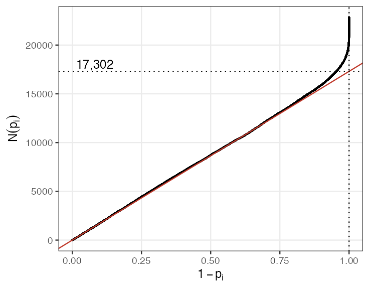
fig_6_15. Reproduces Holmes and Huber (2019), Figure 6.15. Download: PDF · PNGFilling the gap 6.14: why the slope of the Schweder–Spjøtvoll plot estimates \(m_0\) Question 6.17, (6.8), (6.9)
Derivation
\(\E N(p)\)
6.10 The local FDR
Section 6.10 The cartoon of the book's Figure 6.16 (not reproduced) makes the point that a Bayesian, or an empirical Bayesian who learns the prior from many previous cases, can use more than the data of one test. The two-groups model (Efron, 2010) is the formal version for the p-value histogram:
\[ f(p)=\pi_0+(1-\pi_0)f_\text{alt}(p), \tag{6.10} \]the density of the p-values when each hypothesis is null with probability \(\pi_0\) (uniform p-value) and otherwise has p-value density \(f_\text{alt}\). The local false discovery rate at \(p\) and the tail-area false discovery rate are
\[ \fdr(p)=\frac{\pi_0}{f(p)}, \tag{6.11} \] \[ F(p)=\int_0^pf(t)\,\d t, \tag{6.12} \] \[ \Fdr(p)=\frac{\pi_0\,p}{F(p)}. \tag{6.13} \]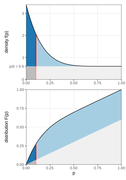
fig_6_17. Reproduces Holmes and Huber (2019), Figure 6.17. Download: PDF · SVGDefinition 6.3 (two-groups model) Section 6.10, (6.10)
Hypotheses are independent draws: \(H_i\sim\Bern(1-\pi_0)\) (1 = non-null), and \(p_i\given H_i=0\sim\Unif(0,1)\), \(p_i\given H_i=1\sim f_\text{alt}\). The marginal density of \(p_i\) is (6.10).
Filling the gap 6.15: what fdr and Fdr are, and how they relate to the FDR Section 6.10, (6.11)–(6.13)
Result 6.7 (local and tail-area fdr in the two-groups model)
(a) \(\fdr(p)=\Prob(H=0\given P=p)\) and \(\Fdr(t)=\Prob(H=0\given P\le t)\). (b) \(\Fdr(t)=\frac1{F(t)}\int_0^t\fdr(s)f(s)\,\d s\), the average of fdr over \([0,t]\) weighted by \(f\). (c) If \(f_\text{alt}\) is non-increasing, then \(\fdr\) is non-decreasing and \(\Fdr(t)\le\fdr(t)\). (d) For \(m\) hypotheses from the model, the rule "reject when \(p_i\le t\)" has positive FDR \(\E[V/R\given R>0]=\Fdr(t)\) (Storey, 2003), and \(\FDR=\Fdr(t)\,\Prob(R>0)\).
Proof
(a) Bayes' theorem with prior \(\pi_0\) and likelihoods 1 (null) and \(f_\text{alt}(p)\): \(\Prob(H=0\given P=p)=\pi_0\cdot1/f(p)\). With events: \(\Prob(H=0\given P\le t)\)
(b) \(\fdr(s)f(s)=\pi_0\), so \(\int_0^t\fdr(s)f(s)\,\d s=\pi_0t\); divide by \(F(t)=\int_0^tf\).
(c) \(f=\pi_0+(1-\pi_0)f_\text{alt}\) is non-increasing, so \(\fdr=\pi_0/f\) is non-decreasing; an \(f\)-weighted average of a non-decreasing function over \([0,t]\) is at most its value at the right end.
(d) Given \(R=r>0\) and given which hypotheses are rejected, each rejected hypothesis is null independently with probability \(\Prob(H=0\given P\le t)=\Fdr(t)\) (the pairs \((H_i,p_i)\) are independent). So \(\E[V\given R=r]=r\,\Fdr(t)\), \(\E[V/R\given R=r]=\Fdr(t)\) for every \(r>0\), hence \(\E[V/R\given R>0]=\Fdr(t)\), and \(\FDR=\E[V/R\given R>0]\Prob(R>0)\). ∎
The numbers of Figure 6.17: \(f(0.1)=0.6+0.4\times7\times0.9^6=2.088\), \(\fdr(0.1)=0.287\), \(F(0.1)=0.06+0.4(1-0.9^7)=0.269\), \(\Fdr(0.1)=0.223\le\fdr(0.1)\). Note that the p-value cut-off 0.1 is neither: a hypothesis with \(p=0.1\) is null with probability 0.29 in this model, and in another model (smaller \(\pi_0\), stronger alternatives) the same p-value could mean 0.05 or 0.6.
The packages qvalue and fdrtool fit the two-groups model to data. fdrtool (Strimmer, 2008) estimates \(\pi_0\) (it calls it eta0) as 0.8823 for the airway p-values, matching the book; this estimate is below 1 because it fits a null to the whole distribution rather than counting \(p>0.5\).
Question 6.18
What do the plots produced by fdrtool show?
Solution
Three panels: the histogram of the p-values with the fitted null component (height eta0) and the fitted mixture density; the fitted distribution functions; and the estimated tail-area Fdr (q-values) and local fdr as functions of the p-value. They are the data versions of the two panels of Figure 6.17, plus the two error-rate curves.
Question 6.19
What does "empirical" in empirical Bayes stand for?
Solution
The prior is estimated from the data instead of being chosen beforehand. In the two-groups model, \(\pi_0\) and \(f_\text{alt}\) play the role of the prior; they cannot be learned from one test but can be from thousands of parallel tests, and the posterior quantities (fdr, Fdr) are then computed with the estimated prior.
6.10.1 Local versus total
Section 6.10.1 The FDR and Fdr are properties of a set of rejections (an average over all of them); the fdr is a property of one hypothesis at the margin. By Result 6.7(b) the first is an average of the second.
Question 6.20
Is there an analogy with total and marginal cost in economics?
Solution
Yes. The expected number of false discoveries among the rejections \(p\le t\) is \(m\pi_0t\), the "total cost"; Fdr is the average cost per discovery, \(m\pi_0t/(mF(t))\). The marginal cost of extending the threshold from \(t\) to \(t+\d t\) is the extra false discoveries per extra discovery, \(\pi_0\,\d t/(f(t)\,\d t)=\fdr(t)\). As with average and marginal costs, the marginal cost is usually higher than the average: by Result 6.7(c), the last discoveries admitted at a threshold are null with a probability above the Fdr of the whole set.
6.10.2 Terminology
Section 6.10.2 The book advises against "multiple testing correction" and "adjusted p-values": BH output is not a p-value of any test, Fdr and FDR are set properties, and fdr depends on modelling assumptions. The adjusted p-values of Filling the gap 6.13 are best read as "the smallest FDR level at which this hypothesis would be in the rejected set".
6.11 Independent hypothesis weighting
Section 6.11 BH and the two-groups model treat the hypotheses as exchangeable: they only see the p-values. Often a second statistic, a covariate, tells us in advance which tests can have power. For RNA-Seq, genes with more reads have a better signal-to-noise ratio; DESeq2's baseMean is the mean of the normalised counts over the 8 samples (708.6 for the first gene). It ranges from 0.09 to 325,663 (Figure 6.18), and no small p-values occur among the genes with low counts (Figure 6.19).
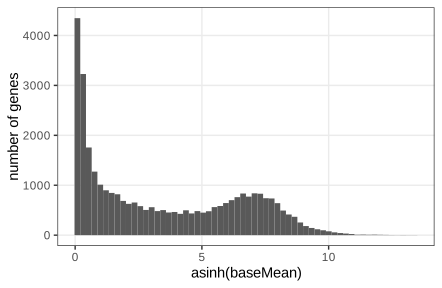
fig_6_18. Reproduces Holmes and Huber (2019), Figure 6.18. Download: PDF · SVG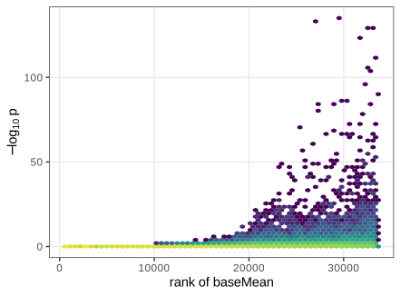
fig_6_19. Reproduces Holmes and Huber (2019), Figure 6.19. Download: PDF · SVGQuestion 6.21
Why the asinh transformation in Figure 6.18? What do no transformation, the logarithm and the shifted logarithm give?
Solution
baseMean spans six orders of magnitude, so without transformation nearly all genes fall into the first bin. \(\operatorname{asinh}(x)=\log(x+\sqrt{x^2+1})\) is about \(\log(2x)\) for large \(x\) and about \(x\) near 0, and it is defined at 0. The logarithm gives nearly the same picture here (all baseMean are positive after removing the untested genes) but fails at zero counts; \(\log(x+c)\) behaves like asinh with the choice of \(c\) deciding where the transition from linear to logarithmic happens.
Question 6.22
Why \(-\log_{10}\) for the p-values and the rank for baseMean in Figure 6.19?
Solution
The interesting p-values are tiny and differ by orders of magnitude; \(-\log_{10}\) spreads them out (and puts the strongest evidence at the top). The rank makes the x-axis uniform: every vertical slice contains the same number of genes, so the hexagon counts are comparable along the axis and the transition is not squeezed into one corner as on the raw scale.
The book splits the genes into six strata of equal size at the sextiles of baseMean (rounded to two significant digits) and looks at the p-value histogram and the distribution function within each (Figures 6.20 and 6.21).
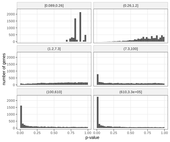
fig_6_20 and strata_of. Reproduces Holmes and Huber (2019), Figure 6.20. Download: PDF · SVG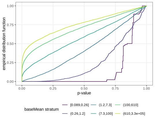
fig_6_21. Reproduces Holmes and Huber (2019), Figure 6.21. Download: PDF · SVGFitted separately, the strata would have very different \(\pi_0\) and \(f_\text{alt}\): in the lowest strata essentially all p-values come from the null (and from a discrete, super-uniform null), while the peak at 0 grows with the counts. The \(\hat\pi_0(0.5)\) of the six strata are 2.00, 1.78, 1.20, 0.82, 0.54 and 0.43.
Filling the gap 6.16: independent filtering, and why it keeps the error control Section 6.11 (the requirement that the covariate be independent of the p-values under the null)
Derivation
The simplest use of the covariate is to drop the hypotheses that cannot be rejected anyway, then run BH on the rest. Suppose that for every true null \(i\), the filter statistic \(U_i\) is independent of \(p_i\), and the pairs \((U_i,p_i)\) are independent across hypotheses. Conditionally on the set \(\mathcal F\) of hypotheses that pass the filter (a function of the \(U\)'s), the null p-values in \(\mathcal F\) are still independent and uniform, and independent of the other p-values in \(\mathcal F\). So Result 6.6 applies conditionally: \(\E[\FDP\given\mathcal F]=\varphi\,m_0(\mathcal F)/|\mathcal F|\le\varphi\), and taking expectations, FDR \(\le\varphi\). Filtering raises power because the BH line \(\varphi i/|\mathcal F|\) is steeper when \(|\mathcal F|\) is smaller, while (if the filter removes mostly nulls) the number of discoverable genes is unchanged (Bourgon, Gentleman and Huber, 2010).
When is the filter independent of the p-value? For the two-sample t-test with normal data, a filter on the overall mean or the overall variance (computed ignoring the labels) qualifies: under the null all \(N\) values are i.i.d. \(\N(\mu,\sigma^2)\); the pair (overall mean, overall sum of squares) is a complete sufficient statistic for \((\mu,\sigma^2)\), and \(t\) is ancillary (its distribution does not depend on \((\mu,\sigma^2)\), since \(t\) is unchanged by \(x\mapsto a+bx\), \(b>0\)); by Basu's theorem they are independent. A filter on \(|m_1-m_2|\) is not independent: it selects null genes with large \(|t|\). In a simulation (20,000 null genes, 4 + 4 samples), null p-values passing a filter on the overall variance remain uniform (KS p = 0.59), while those passing a filter on \(|m_1-m_2|\) have \(\Prob(p\le0.05)=0.080\). For count data and baseMean, independence holds approximately.
On the airway data, keeping the 22,853 genes with baseMean \(\ge1\) raises the BH rejections at \(\varphi=0.1\) from 4,099 to 4,558. ∎
Independent hypothesis weighting (IHW; Ignatiadis et al., 2016; Ignatiadis and Huber, 2021) generalises filtering (weights 0 or a constant) to continuous weights. With ihw(pvalue, baseMean, alpha = 0.1) it rejects 4,892 hypotheses, against 4,099 for BH.
Algorithm 6.3 (weighted BH and IHW) Section 6.11
- Choose non-negative weights \(w_1,\dots,w_m\) with \(\sum_iw_i=m\).
- Apply Algorithm 6.2 to the weighted p-values \(q_i=p_i/w_i\) (\(q_i=\infty\) if \(w_i=0\)): reject \(i\) when \(p_i\le\varphi\,w_iR/m\).
- IHW: bin the covariate into strata, split the hypotheses at random into folds, and for each fold choose one weight per stratum (to maximise the rejections) using only the other folds; then apply step 2 to all hypotheses.
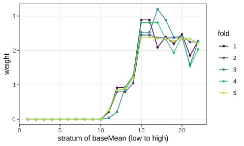
ihw, one curve per fold (5 folds). Low-count strata get weight 0, high-count strata about 2.4. Code: fig_6_22 and ihw_result. Reproduces Holmes and Huber (2019), Figure 6.22. Download: PDF · SVGQuestion 6.23
Why does Figure 6.22 show 5 curves?
Solution
IHW uses 5 folds by default. The weights of the hypotheses in one fold are learned from the other four folds only (cross-weighting), so each fold has its own weight curve. This keeps each hypothesis's weight independent of its own p-value, the condition of Result 6.8.
Filling the gap 6.17: weighted BH controls the FDR, and why the weights must not see the p-values Section 6.11
Result 6.8 (weighted BH; Genovese, Roeder and Wasserman, 2006)
Under the independence assumptions of Result 6.6, with fixed weights \(w_i\ge0\), \(\sum_iw_i=m\), weighted BH has
\[ \FDR\le\frac{\varphi}{m}\sum_{i\in\mathcal H_0}w_i\le\varphi, \]with equality in the first inequality when \(\varphi w_i\le1\) for all null \(i\) and the null p-values are uniform.
Proof
Repeat the proof of Result 6.6 with \(q_i=p_i/w_i\). Hypothesis \(i\) is rejected when \(p_i\le\varphi w_iR/m\). The leave-one-out lemma holds verbatim for the \(q\)'s (replace \(q_i\) by 0). So \(\E[\ind\{R=k\}\ind\{p_i\le\varphi w_ik/m\}]\)
The proof needs the weights to be fixed, or at least independent of the null p-values. Weights tuned on the same p-values they are applied to (choose the weights that maximise the number of rejections) break this: the optimiser favours strata where nulls happen to have small p-values, and the FDR can exceed \(\varphi\). IHW's cross-weighting restores the independence: the weights of fold \(k\) are a function of the other folds, independent of the p-values in fold \(k\) (Ignatiadis and Huber, 2021). In a simulation, fixed weights 0.5 and 1.5 give a simulated FDR of 0.0702 against the formula's 0.0700, and weighted BH with the weights exported from ihw reproduces its 4,892 rejections exactly. A good covariate is (i) independent of the p-values under the null and (ii) informative about \(\pi_0\) or the power, which Figures 6.18–6.21 let us check.
Summary
- A test fixes a rejection region of null probability \(\alpha\) before the data are seen. A p-value is valid when \(\Prob_0(p\le\alpha)\le\alpha\); it is uniform for a continuous statistic and conservative for a discrete one.
- The t distribution is exact under independent normal data with a common variance; the permutation test is exact under exchangeability alone. Dependence between observations (duplicates, technical replicates) invalidates both.
- Choices made after seeing the data inflate the false positive rate; optional stopping drives it to 1.
- For many tests, Bonferroni controls the FWER under any dependence but has low power; Benjamini–Hochberg controls the FDR at \(\pi_0\varphi\) under independence, by a short leave-one-out argument.
- The p-value histogram is a mixture of a flat null part and a peak of alternatives; it estimates \(\pi_0\) and diagnoses problems (here: the discreteness of low counts). In the two-groups model, fdr is the posterior probability of the null for one hypothesis, Fdr the average over a rejection set.
- A covariate independent of the null p-values can be used to filter or weight hypotheses, with the FDR guarantee intact if the weights do not see the p-values they are applied to.
Exercises
The exercises of Holmes and Huber (2019), Section 6.14, restated in my own words, with solutions (hidden).
Exercise 6.1. Find a multiple-testing application in your own field, plot the p-value histogram, and look for informative covariates; plot the stratified histograms.
Solution
A worked example is the airway analysis of these notes: the overall histogram (Figure 6.12) shows a clear peak at 0 and a discreteness artefact at the right; stratifying by the mean count (Figures 6.20, 6.21) shows that the covariate is informative (\(\hat\pi_0\) falls from about 1 to 0.43 across strata) and plausibly independent of the null p-values (the right halves of the histograms of the high strata are flat). Typical covariates elsewhere: minor allele frequency in genetic association studies, distance to the transcription start site for ChIP-seq peaks, the number of reads per site in methylation data, and the sample size behind each test in meta-analyses. Check that the covariate does not change the null distribution: the stratified histograms should be flat on the right in every stratum.
Exercise (unnumbered). Why do mathematical statisticians focus so much on the null hypothesis of a test, compared to the alternative?
Solution
Because the null is the only fully specified model: it is simple (or has a known invariance, as in permutation tests), so the distribution of the statistic, and therefore the type I error, can be computed and guaranteed. The alternative is usually composite (any effect size, any direction, any shape), so the power is a function, not a number, and cannot be controlled without assumptions. The theory therefore controls the error that can be controlled, \(\alpha\), and among tests with that guarantee looks for good power (Result 6.2).
Exercise 6.2. Can we ever prove that the null hypothesis is true? Or that the alternative is true?
Solution
Not from finite noisy data. A non-rejection is compatible with the null and with every alternative close enough to it (Question 6.1). What can be shown is that the effect is small: an equivalence test takes "|effect| \(\ge\delta\)" as the null and rejects it when a confidence interval lies inside \((-\delta,\delta)\) (two one-sided tests at level \(\alpha\)). A rejection of the null does not prove the alternative either; it says that data like these would be rare under the null, with a controlled error rate \(\alpha\). Bayesian analyses give posterior probabilities of each hypothesis, which require priors.
Exercise 6.3. Simulate data with true nulls only, with replicates that move from fully independent to highly correlated as a parameter varies, and check type I error control as a function of that parameter.
Solution
Design. Two groups of 4 plants, each plant measured twice; the two measurements of a plant have correlation \(\rho\): \(x=\sqrt\rho\,u_\text{plant}+\sqrt{1-\rho}\,e\) with independent standard normal \(u,e\). The naive two-sample t-test treats the 16 values as independent (14 df). Note that a correlation shared by all values of a gene would not matter (it cancels in \(m_1-m_2\)); it is correlation within a group that pretends to be replication.
Result (20,000 data sets per \(\rho\)): rejection rate at 5% is 0.052 for \(\rho=0\), 0.118 for \(\rho=0.5\), 0.214 for \(\rho=1\). At \(\rho=1\) the data are exact duplicates and Filling the gap 6.7 gives the exact value: \(t_2=t\sqrt{14/6}\) with \(t\sim t_6\), so the size is \(2\Prob(T_6>t_{14,0.975}/\sqrt{14/6})=0.2099\), which the simulation matches. A p-value histogram of these tests rises towards 0 with \(\rho\). Averaging the two measurements per plant restores the exact 5% for every \(\rho\).
Exercise 6.4. Find an example in the literature that looks like p-value hacking, outcome switching or HARKing.
Solution
No mathematical answer. Useful signs: a primary outcome in the paper that differs from the registered one (trial registries make this checkable); many reported subgroup analyses with one significant; p-values clustered just below 0.05 across a literature (Head et al., 2015, study the distribution of reported p-values for exactly this "bump"); sample sizes that are not justified in advance. When you find one, ask what the false positive rate of the procedure that was actually followed is, as in Filling the gap 6.9.
Exercise 6.5. The FDR controls an average. Are there methods for worst-case control?
Solution
Yes. (1) FWER control bounds the probability of even one false discovery (Bonferroni, Result 6.5). Holm's step-down procedure is uniformly better: with \(p_{(1)}\le\dots\le p_{(m)}\), reject \(p_{(1)},p_{(2)},\dots\) as long as \(p_{(j)}\le\alpha/(m-j+1)\) and stop at the first failure. Proof of FWER control: let \(j^*\) be the rank of the smallest null p-value. At most \(m-m_0\) p-values precede it, so \(j^*\le m-m_0+1\), and a false rejection requires it to pass its threshold \(\alpha/(m-j^*+1)\le\alpha/m_0\); by the union bound \(\Prob(\min_{i\in\mathcal H_0}p_i\le\alpha/m_0)\le\alpha\). (2) FDP exceedance control bounds \(\Prob(\FDP>\gamma)\le\alpha\) (Lehmann and Romano, 2005), a statement about the realised proportion in this experiment rather than its mean. (3) Simultaneous confidence bounds for the FDP of every possible selection (Goeman and Solari, 2011) allow choosing the rejection set after looking, with a guarantee.
Exercise 6.6. What are the memory and time complexity of BH and of IHW? Measure them as functions of \(m\) and fit a power law on a log-log plot.
Solution
BH: sorting dominates, \(O(m\log m)\) time; the running minimum of
p.adjustis \(O(m)\); memory is \(O(m)\) (a few vectors of length \(m\)). Timingp.adjust(p, "BH")for \(m=10^4,\dots,10^7\) on the build machine gives a log-log slope of 1.13, consistent with \(m\log m\) over this range (the \(\log m\) factor and cache effects push the slope slightly above 1). IHW: for each of the \(K\) folds it computes stratified empirical distribution functions (\(O(m\log m)\)) and solves an optimisation over the \(B\) strata weights (a convex problem whose size depends on \(B\) and the grid of regularisation values, not on \(m\)), then one weighted BH: \(O(Km\log m)\) time plus a term independent of \(m\), and \(O(m)\) memory. The method of measurement:microbenchmarkorsystem.timeover a grid of \(m\),lm(log(time) ~ log(m)).
Demonstrations for this chapter
Each demonstration runs in the browser, with seeded random numbers, and links back to these notes. Their computations were compared with the R code.
| Demonstration | What you can see | Agreement with R |
|---|---|---|
| The exact binomial test | Rejection regions of different shapes, the exact p-value, power against the true bias and as a function of n, the null distribution of a discrete p-value. Presets: 1 the book's coin (Fig. 6.7); 2 equal tails; 3 one-sided; 4 power and sample size; 5 discrete p-values. | p-value, region sizes and power agree to 7 digits. |
| The t-test and the permutation test | PlantGrowth: exact permutation distribution from all 184,756 splits, Monte Carlo p-values, t, difference of means and Welch, one- and two-sided, duplicated data. Presets: 1 ctrl vs trt2 (Figs. 6.9, 6.10); 2 one-sided; 3 Monte Carlo; 4 trt1 vs trt2; 5 duplicated data. | t, p and the exact permutation counts identical (8,930 of 184,756). |
| P-value hacking | Optional stopping with simulated null studies and the exact false positive rate; the rate as the patience grows; the best of K correlated statistics. Presets: 1 every observation; 2 every 10; 3 up to 1,000; 4 best of 5; 5 correlated. | Exact rates agree to 10 digits (0.2763600171). |
| Multiple testing on the airway data | The p-value histogram and \(\hat\pi_0\), BH against Bonferroni, baseMean strata and IHW weights, a simulation of the FDR of BH. Presets: 1 visual FDR (Fig. 6.13); 2 BH (Fig. 6.14); 3 strata and IHW; 4 FDR simulation; 5 all nulls. | BH 4,099, Bonferroni 1,444, weighted BH 4,892, \(\hat\pi_0=1.129284\), strata sizes: identical. |
The R code that produces every figure of this page is code/ch06_testing.R (see the code index).
References
- Holmes, S. and Huber, W. (2019). Modern Statistics for Modern Biology. Cambridge University Press. Chapter 6.
- Armitage, P., McPherson, C. K. and Rowe, B. C. (1969). Repeated significance tests on accumulating data. Journal of the Royal Statistical Society: Series A, 132(2), 235–244.
- Benjamini, Y. and Hochberg, Y. (1995). Controlling the false discovery rate: a practical and powerful approach to multiple testing. Journal of the Royal Statistical Society: Series B, 57(1), 289–300.
- Benjamini, Y. and Yekutieli, D. (2001). The control of the false discovery rate in multiple testing under dependency. The Annals of Statistics, 29(4), 1165–1188. doi:10.1214/aos/1013699998.
- Bourgon, R., Gentleman, R. and Huber, W. (2010). Independent filtering increases detection power for high-throughput experiments. Proceedings of the National Academy of Sciences, 107(21), 9546–9551. doi:10.1073/pnas.0914005107.
- Clopper, C. J. and Pearson, E. S. (1934). The use of confidence or fiducial limits illustrated in the case of the binomial. Biometrika, 26(4), 404–413. doi:10.1093/biomet/26.4.404.
- Efron, B. (2010). Large-Scale Inference: Empirical Bayes Methods for Estimation, Testing, and Prediction. Cambridge University Press.
- Genovese, C. R., Roeder, K. and Wasserman, L. (2006). False discovery control with p-value weighting. Biometrika, 93(3), 509–524.
- Goeman, J. J. and Solari, A. (2011). Multiple testing for exploratory research. Statistical Science, 26(4), 584–597.
- Head, M. L., Holman, L., Lanfear, R., Kahn, A. T. and Jennions, M. D. (2015). The extent and consequences of p-hacking in science. PLoS Biology, 13(3), e1002106. doi:10.1371/journal.pbio.1002106.
- Himes, B. E. et al. (2014). RNA-Seq transcriptome profiling identifies CRISPLD2 as a glucocorticoid responsive gene that modulates cytokine function in airway smooth muscle cells. PLoS ONE, 9(6), e99625. doi:10.1371/journal.pone.0099625.
- Hoeffding, W. (1951). A combinatorial central limit theorem. The Annals of Mathematical Statistics, 22(4), 558–566.
- Ignatiadis, N., Klaus, B., Zaugg, J. B. and Huber, W. (2016). Data-driven hypothesis weighting increases detection power in genome-scale multiple testing. Nature Methods, 13, 577–580.
- Ignatiadis, N. and Huber, W. (2021). Covariate powered cross-weighted multiple testing. Journal of the Royal Statistical Society: Series B, 83, 720–751. doi:10.1111/rssb.12411.
- Lehmann, E. L. and Romano, J. P. (2005). Generalizations of the familywise error rate. The Annals of Statistics, 33(3), 1138–1154.
- Love, M. I., Huber, W. and Anders, S. (2014). Moderated estimation of fold change and dispersion for RNA-seq data with DESeq2. Genome Biology, 15, 550. doi:10.1186/s13059-014-0550-8.
- Phipson, B. and Smyth, G. K. (2010). Permutation p-values should never be zero: calculating exact p-values when permutations are randomly drawn. Statistical Applications in Genetics and Molecular Biology, 9(1), Article 39. doi:10.2202/1544-6115.1585.
- Schweder, T. and Spjøtvoll, E. (1982). Plots of p-values to evaluate many tests simultaneously. Biometrika, 69(3), 493–502. doi:10.1093/biomet/69.3.493.
- Simes, R. J. (1986). An improved Bonferroni procedure for multiple tests of significance. Biometrika, 73(3), 751–754. doi:10.1093/biomet/73.3.751.
- Storey, J. D. (2002). A direct approach to false discovery rates. Journal of the Royal Statistical Society: Series B, 64(3), 479–498. doi:10.1111/1467-9868.00346.
- Storey, J. D. (2003). The positive false discovery rate: a Bayesian interpretation and the q-value. The Annals of Statistics, 31(6), 2013–2035. doi:10.1214/aos/1074290335.
- Storey, J. D., Taylor, J. E. and Siegmund, D. (2004). Strong control, conservative point estimation and simultaneous conservative consistency of false discovery rates: a unified approach. Journal of the Royal Statistical Society: Series B, 66(1), 187–205.
- Strimmer, K. (2008). fdrtool: a versatile R package for estimating local and tail area-based false discovery rates. Bioinformatics, 24(12), 1461–1462.
- Wasserstein, R. L. and Lazar, N. A. (2016). The ASA's statement on p-values: context, process, and purpose. The American Statistician, 70(2), 129–133. doi:10.1080/00031305.2016.1154108.
Data: PlantGrowth (R datasets), airway (Bioconductor), analysed with DESeq2, IHW and fdrtool. Every number in the text comes from the course R code; the figures are drawn by it.